On a quadratic form associated with a surface automorphism and its applications to Singularity Theory

Abstract.

We study the nilpotent part $N^{\prime}$ of a pseudo-periodic automorphism $h$ of a real oriented surface with boundary $\Sigma$. We associate a quadratic form $Q$ defined on the first homology group (relative to the boundary) of the surface $\Sigma$. Using the twist formula and techniques from mapping class group theory, we prove that the form $\tilde{Q}$ obtained after killing ${\ker N}$ is positive definite if all the screw numbers associated with certain orbits of annuli are positive. We also prove that the restriction of $\tilde{Q}$ to the absolute homology group of $\Sigma$ is even whenever the quotient of the Nielsen-Thurston graph under the action of the automorphism is a tree. The case of monodromy automorphisms of Milnor fibers $\Sigma=F$ of germs of curves on normal surface singularities is discussed in detail, and the aforementioned results are specialized to such situation. Moreover, the form $\tilde{Q}$ is computable in terms of the dual resolution or semistable reduction graph, as illustrated with several examples. Numerical invariants associated with $\tilde{Q}$ are able to distinguish plane curve singularities with different topological types but same spectral pairs. Finally, we discuss a generic linear germ defined on a superisolated surface. In this case the plumbing graph is not a tree and the restriction of $\tilde{Q}$ to the absolute monodromy of $\Sigma=F$ is not even.

Introduction

We study the nilpotent part of pseudo-periodic automorphisms of real oriented surfaces with boundary. The monodromy of families of algebraic curves and the geometric monodromy of hypersurfaces on germs of normal surface singularities are examples of such automorphims. Our motivation comes indeed from the latter case. Note also that the study of automorphisms of surfaces has appeared on several recent works on arithmetic and tropical geometry, see for instance [15] and [2].

We associate a quadratic form with a pseudo-periodic automorphism $h$ of a real oriented surface $\Sigma$ with boundary, i.e., $\partial\Sigma\neq\emptyset$. Let $e\in\mathbb{N}$ be the least common multiple of the orders of $h$ restricted to each periodic piece in its Nielsen-Thurston decomposition. We consider the $\mathbb{Z}$-linear operators

$$N:H_{1}(\Sigma,\partial\Sigma;\mathbb{Z})\longrightarrow H_{1}(\Sigma;\mathbb{Z})\text{ and }N^{\prime}:H_{1}(\Sigma;\mathbb{Z})\longrightarrow H_{1}(\Sigma;\mathbb{Z}),$$

given by $[\gamma]\mapsto{[h^{e}(\gamma)-\gamma]}$, and we associate with them the symmetric bilinear form

$$Q:H_{1}(\Sigma,\partial\Sigma;\mathbb{Z})\times H_{1}(\Sigma,\partial\Sigma;\mathbb{Z})\longrightarrow\mathbb{Z},\hskip 14.22636pt\hbox{ defined by }\hskip 14.22636ptQ(\alpha,\beta):=\left\langle N\alpha,\beta\right\rangle,$$

and also

$$\tilde{Q}:\frac{H_{1}(\Sigma,\partial\Sigma;\mathbb{Z})}{\ker N}\times\frac{H_{1}(\Sigma,\partial\Sigma;\mathbb{Z})}{\ker N}\longrightarrow{\mathbb{Z}},$$

where $\left\langle\ ,\ \right\rangle:H_{1}(\Sigma;\mathbb{Z})\times H_{1}(\Sigma,\partial\Sigma;\mathbb{Z})\longrightarrow\mathbb{Z}$ denotes the usual intersection product. In a similar way we can define a symmetric bilinear form $Q^{\prime}$ on $H_{1}(\Sigma;\mathbb{Z})$.

The $\mathbb{Z}$-linear operator $N$ and the quadratic form $Q$ are designed to recover information of the unipotent part of $h_{\ast}$. The linear operator $N$ is defined as a variation operator for $h_{\ast}^{e}$ and therefore the contributions to $H_{1}(\Sigma,\partial\Sigma,\mathbb{Z})$ coming from the periodic pieces of Nielsen-Thurston decomposition of $h$ are killed by $N$. The image of $N$ on the other hand can be represented by a collection of disjoint simple closed oriented curves on $\Sigma$ with the property that each of those simple closed curves do not intersect the homology of the periodic pieces but goes through at least one annular neighborhood of a separating curve in the Nielsen-Thurston decomposition of $h$. Note that, at least in the singularity theory setting and according to the formula for the characteristic polynomial of $h_{\ast}$ in $H_{1}(\Sigma,\mathbb{Z})/\ker N^{\prime}$ (see Section 3.4), the unipotent part of $h$ comes from the separating nodes, and paths joining pairs of them. These relate to the aforementioned annuli. The quadratic form $Q$ encodes the intersection of the elements of $H_{1}(\Sigma,\partial\Sigma,\mathbb{Z})$ with their images under $N$.

The basic techniques for the study of automorphisms of real oriented surfaces are the Nielsen-Thurston classification and the mapping class group. The main references are the book of Matsumoto and Montesinos [18] and the book of Farb and Margalit [7]. We use these techniques to give explicit formulas of $N$ and $\tilde{Q}$, and sufficient conditions for $\tilde{Q}$ being positive definite and being even. Definiteness of a quadratic form is an important property related to a notion of convexity and, in the algebraic setting, to the Hodge index theorem.

Let $\mathcal{C}$ be a collection of pairwise disjoint simple closed curves on $\Sigma$ determining the canonical form or decomposition of the pseudo periodic automorphism $h$, see Theorem 1.2. Let $v,w\in H_{1}(\Sigma,\partial\Sigma;\mathbb{Z})$ and let $\gamma_{v},\gamma_{w}$ oriented curves on $\Sigma$ representing these classes. For $C\in\mathcal{C}$, let $T_{C}$ be a tubular neighborhood of the curve $C$, and let $s_{C}=\operatorname{sc}(h^{e},T_{C})$ be the screw number associated to the annulus $T_{C}$, see Definition 1.4, and Lemma 1.8. The main results about $N$ and $\tilde{Q}$ are Theorem 2.5, 2.8 and formulas (2.9) and (2.10). These statements can be summarized as follows.

Theorem A.

The operator $N$ and the quadratic form $\tilde{Q}$ are given by the formulas

$$N(v)=\sum_{C\in\mathcal{C}}s_{C}\langle[C],v\rangle[C]\quad\hbox{ and }\quad\tilde{Q}(v,w)=\sum_{C\in\mathcal{C}}s_{C}\langle[C],v\rangle\langle[C],w\rangle.$$

The bilinear form $\tilde{Q}$ is positive definite if all the screw numbers associated to non-nullhomotopic curves $C$ are positive and $Q^{\prime}$ is even whenever the quotient of the Nielsen-Thurston graph $G(h)$ under the action induced by $h$ is a tree.

We can interpret this theorem in the following way. The space $H_{1}(\Sigma,\partial\Sigma;\mathbb{Z})/\ker N$ can be identified with the homology in degree $1$ of the Nielsen-Thurston graph of the monodromy automorphism relative to the vertices coming from the boundary. The screw numbers of $h^{e}$ define a diagonal positive definite form in the group of $1$-chains of the Nielsen-Thurston graph. The bilinear form $\tilde{Q}$ is identified with the restriction of this form to the above relative homology.

The role of quadratic forms in Singularity theory has been surveyed by Wall [25], in the normal surface case, and Hertling [12]. If $h$ is the geometric monodromy of a germ of hypersurface on a normal surface singularity and $\Sigma=F$ is the corresponding Milnor fiber, then the hypothesis on the screw numbers in the above theorem is satisfied, see Theorem 3.6. The reasons behind the positivity of the screw numbers $s_{C}$ are the twist formula Proposition 3.4, and the fact that the resolution data $m_{i}$ are always positive, see Section 3.1. Alternatively and due to a remark of Mumford [19, II, (b), (ii)], the positivity of the resolution data $m_{i}$ can be understood as a consequence of the negative definiteness of the intersection matrix of a resolution, see Remark 3.2. The hypothesis about the shape of the quotient of the Nielsen-Thurston graph $G(h)$ under the action induced by $h$ in the above theorem is satisfied for plane curve singularities, see 3.12.

Furthermore, in the case of geometric monodromies of hypersurfaces on germs of normal surfaces, there is an equivalence between the dual graph $\Gamma_{\!\textrm{ss}}$ of the semistable reduction, and the Nielsen-Thurston graph of $h$, see Lemma 3.14. In particular, there is a map associating to a closed path $\alpha$ in $F$ its image in the dual graph $\Gamma_{\!\textrm{ss}}$ of the semistable reduction. This map induces isomorphisms

$$\frac{H_{1}(F;\mathbb{Z})}{W_{1}}\longrightarrow H_{1}(\Gamma_{\!\textrm{ss}};\mathbb{Z})\quad\hbox{ and }\quad\frac{H_{1}(F,\partial F;\mathbb{Z})}{\ker N}\longrightarrow H_{1}(\Gamma_{\!\textrm{ss}},\mathcal{D};\mathbb{Z})\text{, see page\leavevmode\nobreak\ \ref{calD} for }W_{1}\text{ and }\mathcal{D},$$

and allows us to perform very explicit computations of the form $\tilde{Q}$ in particular examples, see Section 4. In particular, we show that numerical invariants associated to $\tilde{Q}$ are able to distinguish classic examples of pairs of plane curve singularities with different topological type but same spectral pairs, due to Schrauwen, Steenbrink, and Stevens, see Example 4.5. In [5] Du Bois and Michel gave two infinite families of reducible plane singularities (all members of both families consist of two branches) which are not topologically equivalent but have the same Seifert form. The members of both families have asymptotically big Milnor numbers. Therefore their Seifert forms become asymptotically complicated too. We compute in Example 4.6 the forms $\tilde{Q}$ associated with both families. It is worth mentioning that for those families $\tilde{Q}$ is always defined on an abelian group of rank $4$. Our computation show that for pairs of members of these families of singularities (with the same Seifert form) the forms $\tilde{Q}$ are equivalent. This is not surprising, as pointed out by a referee (to whom we are strongly grateful), since $\tilde{Q}$ depends on the Seifert form, see [26, §10] or [1, §2.3]. Nevertheless, note that while $\tilde{Q}$ is weaker than the Seifert form it is also computationally much simpler. The examples of Schrauwen, Steenbrink, and Stevens, which have equal Seifert forms over $\mathbb{R}$, have no equivalent forms $\tilde{Q}$, hence the real Seifert form does not determined our bilinear form. For the examples of Du Bois and Michel, we prove the equality in the same way as they did, finding suitable bases where the matrices coincide. Supplementary details (and possible verification) on the examples are provided in the link https://github.com/enriqueartal/QuadraticFormSingularity which can be executed using Binder.

Finally, a few words linking the results presented here with a future project. The operator $N$ and the quadratic form $\tilde{Q}$ studied in this paper aim to describe the topological part of the multiplication by a germ of holomorphic map $f:(\mathbb{C}^{n+1},0)\to(\mathbb{C},0)$ and of the residue pairing defined on the Jacobian module of $f$. Notice that the multiplication by $f$ map and the residue pairing encode analytic information in contrast to $N$ and $\tilde{Q}$ which encode just topological information.

The multiplication by $f$ map on the jacobian module $\Omega_{f}$ is given by $[gdz]\mapsto[(fg)dz]$. It is a nilpotent map with index $\leq n+1$, and it is trivial if and only if $f$ is right-equivalent to a quasihomogeneous polynomial. Varchenko established that the nilpotent operator of the homological monodromy, and the map $Gr_{\mathcal{V}}\{f\}$, the graded multiplication by $f$ map with respect to the Kashiwara-Malgrange filtration $\mathcal{V}$, have the same Jordan block structure [24].

Using the Grothendieck local duality theorem, one can define a nondegenerate symmetric residue pairing $\operatorname{res}_{f,0}:\Omega_{f}\times\Omega_{f}\rightarrow\mathbb{C}$ as

$$\operatorname{res}_{f,0}([g_{1}dz],[g_{2}dz])=\left(\frac{1}{2\pi i}\right)^{n+1}\int_{\Gamma_{\varepsilon}}\left(\frac{g_{1}(z)g_{2}(z)}{\prod_{j=0}^{n}f_{j}}\right),$$

where $\Gamma_{\varepsilon}$ is a ($n+1$)-real vanishing cycle determined by the partial derivatives $\partial f/\partial z_{j}$, and define the bilinear form $\operatorname{res}_{f,0}(\{f\}\bullet,\bullet)$, which degenerates on $\ker\{f\}$.

It is worthwhile to notice that, motivated by previous results relating the signatures of the residue pairing $\operatorname{res}_{f,0}(\{f\}\bullet,\bullet)$ to indices of vector fields [8], the fourth named author initiated a program to analyze additive expansions of the bilinear forms $\operatorname{res}_{f,0}(\{f\}^{l}\bullet,\bullet)$ and to compare them to some topological bilinear form introduced by Hertling [10, 11], see for instance the results from [3].

1. Nielsen-Thurston theory

Let $\Sigma$ be a real oriented surface with $\partial\Sigma\neq\emptyset$. Assume that $\Sigma$ has genus $g$ and $r$ boundary components. Let $\mathrm{Mod}_{g,r}(\Sigma,\partial\Sigma)$ denote the mapping class group of surface diffeomorphisms of the surface of $\Sigma$ that restrict to the identity on the boundary components and up to isotopy fixing the boundary.

Example 1.1.

Let $\mathcal{D}:\mathbb{S}^{1}\times[-\frac{1}{2},\frac{1}{2}]\rightarrow\mathbb{S}^{1}\times[-\frac{1}{2},\frac{1}{2}]$ be the homeomorphism defined by $\mathcal{D}(x,t)=(x+t,t)$, where $\mathbb{S}^{1}$ is identified with $\mathbb{R}/\mathbb{Z}$. Let $\mathcal{A}$ be an annulus. A homeomorphism $h:\mathcal{A}\rightarrow\mathcal{A}$ is called a right-handed Dehn twist if there exists a parametrization $\eta:\mathbb{S}^{1}\times[-\frac{1}{2},\frac{1}{2}]\rightarrow\mathcal{A}$ such that $h=\eta\circ\mathcal{D}\circ\eta^{-1}$. The mapping class group $\mathrm{Mod}_{0,2}(\mathcal{A},\partial\mathcal{A})$ is isomorphic to $\mathbb{Z}$, and it is generated by a right-handed Dehn twist.

The Nielsen-Thurston classification of mapping classes [7, Theorem 13.2, see also the statement in page $11$] says that for each mapping class one of the following exclusive statements is satisfied.

1. $h$ is periodic, i.e., there exists $n\in\mathbb{N}$ such that $h^{n}=\mathop{\mathrm{id}}\nolimits\in\mathrm{Mod}_{g,r}(\Sigma,\partial\Sigma)$.

2. $h$ is pseudo-Anosov. (The appropiate definition of this notion takes some time and it won’t be used in the present work. We refer the interested reader to [7] for more on this topic.)

3. $h$ is reducible, i.e., there exists a representative $\phi$ of $h$ and a finite union of disjoint simple closed curves that is invariant by $\phi$.

It follows that one can cut up the surface $\Sigma$ along a collection of invariant curves into (maybe disconnected) surfaces such that the restriction of an appropriate representative of $h$ to each of these pieces is either periodic or pseudo-Anosov. When only periodic pieces appear in this decomposition, we say that $h$ is a pseudo periodic mapping class. In this work we only deal with this type of mapping classes.

According to Nielsen-Thurston theory each pseudo periodic mapping class has a nice representative that we call canonical form. This homeomorphism is defined by the following theorem.

Theorem 1.2 (Canonical form, [7, Corollary 13.3]).

Let $h\in\mathrm{Mod}_{g,r}(\Sigma,\partial\Sigma)$ be pseudo periodic. Then there exists a collection $\mathcal{C}$ of pairwise disjoint simple closed curves on $\Sigma$, including curves parallel to all boundary components, a collection $\mathcal{T}$ of pairwise disjoint tubular neighbourhoods $\mathcal{T}_{i}$ of each $C_{i}$ in $\mathcal{C}$, and a representative $\phi:\Sigma\to\Sigma$ of $h$ in $\mathrm{Mod}_{g,r}(\Sigma,\partial\Sigma)$ such that

1. The multicurve $\mathcal{C}$ and the multiannulus $\mathcal{T}$ are invariant by $\phi$, that is, $\phi(\mathcal{C})=\mathcal{C}$, and $\phi(\mathcal{T})=\mathcal{T}$.

2. The automorphism $\phi$ restricted to suitable unions of components of the closure of $\Sigma\setminus\mathcal{T}$ is periodic.

3. If $n$ is a common multiple of the periods of the components of $\Sigma\setminus\mathcal{T}$, then $\phi^{n}$ is the composition of non-trivial (and non necessarily positive) powers of right-handed Dehn-twist along all the curves in $\mathcal{C}$.

Denote by $\mathcal{C}^{+}$ the subcollection of curves of $\mathcal{C}$ that are not parallel to the boundary, which are called separating curves. We will always assume that $\mathcal{C}^{+}$ is minimal.

In the sequel we may identify $h$ and $\phi$ if no confusion is likely.

Remark 1.3.

A. Pichon gives a characterization of pseudo periodic automorphisms corresponding to the geometric monodromy of the Milnor fibration of a germ of a hypersurface on a normal surface as those such that all the powers in (iii) above are positive [21]. We will consider such situation in Section 3 and Section 4.

The behavior of the automorphism $h$ in the collection $\mathcal{T}$ of annuli is described by a rational amount of rotation. The notion of screw numbers, that we define next, measures this amount.

The action of $h$ and its powers partitions the collection $\mathcal{C}$ into orbits of curves. Let $\mathcal{C}_{\ast}:=\{C_{1},\ldots,C_{d}\}\subset\mathcal{C}$ be an orbit of curves defined by $h$. Let $\delta\in\{d,2d\}$, where $\delta=d$ if $h^{d}$ sends $C_{1}$ to $C_{1}$ with the same orientation and $2d$ otherwise. Let $m_{1},m_{2}\in\mathbb{N}$ be the periods of $h$ restricted to the periodic pieces on each side of the orbit and let $n:=\operatorname{lcm}(m_{1},m_{2})$. Then, we have that $h^{n}$ restricted to $\mathcal{T}_{1}$ is an integral power, let us say $\ell$, of a right-handed Dehn twist around $C_{1}$.

Definition 1.4.

With the above notations, we define the screw number of $h$ at the orbit $\mathcal{C}_{\ast}$ by

$$\operatorname{sc}(h,\mathcal{C}_{\ast})=\operatorname{sc}(h,\mathcal{T}_{\ast}):=\frac{\delta\ell}{n}.$$

Remark 1.5.

The screw number is defined for an orbit (by $h$) of simple closed curves. This is because the quantity does not depend on the curve chosen to compute it. In the same way, when it is more convenient, we speak of the screw number at an orbit of annuli or at a given annulus where these are taken to be tubular neighborhoods of an orbit of simple closed curves.

We recall now the notion of intersection product

(1.6) $$\langle\cdot,\cdot\rangle:H_{1}(\Sigma;\mathbb{Z})\times H_{1}(\Sigma,\partial\Sigma;\mathbb{Z})\to\mathbb{Z}$$

on $\Sigma$ that is computed as follows. Firstly, every element $\alpha\in H_{1}(\Sigma;\mathbb{Z})$ can be represented by a disjoint union $\gamma_{\alpha}$ of simple closed curves in $\Sigma$ and any primitive element $\beta\in H_{1}(\Sigma,\partial\Sigma;\mathbb{Z})$ can be represented by a disjoint union of simple closed curves and properly embedded arcs that we denote by $\gamma_{\beta}$. Now, for two such elements $\alpha,\beta$ we can actually define $\langle\alpha,\beta\rangle$ to be the algebraic intersection number of $\gamma_{\alpha}$ and $\gamma_{\beta}$, i.e.,

(1.7) $$\langle\alpha,\beta\rangle:=i(\gamma_{\alpha},\gamma_{\beta}).$$

Finally, one can compute this number by taking representatives of $\gamma_{\alpha}$ and $\gamma_{\beta}$ in their isotopy classes such that they intersect transversely and then one counts $+1^{\prime}s$ and $-1^{\prime}s$ on each intersection point according to the orientation of $\Sigma$. Note that in this way the intersection form is well defined, non degenerate, and that swapping the factors in the domain of the intersection form results in the multiplication by $-1$ on its value.

The next lemma explains the geometric meaning of the screw numbers.

Figure 1.1. The annulus is oriented counterclockwise and induces the orientation on the boundary.

Lemma 1.8.

Let $h$ be a pseudo-periodic automorphism $h:\Sigma\rightarrow\Sigma$. Let $\mathcal{T}_{\ast}$ be an orbit of $d$ annuli by the action of $h$, and let $T$ be an annulus in $\mathcal{T}_{\ast}$.

Let $e\in\mathbb{N}$ be such that $h^{e}|_{\partial T}=\mathop{\mathrm{id}}\nolimits$. Let $I,J\hookrightarrow T$ be two properly embedded, disjoint and oriented arcs with one end on each boundary component of $\partial T$ and let $C$ be the core curve of $T$ suitably oriented.

We have the following:

1. $\operatorname{sc}(h^{e},T)\in\mathbb{N}$;

2. $\operatorname{sc}(h^{e},T)=\frac{e}{d}\cdot\operatorname{sc}(h,T)$;

3. $h^{e}(I)-I=\operatorname{sc}(h^{e},T)\cdot C\in H_{1}(F,\mathbb{Z})$.

4. $\langle h^{e}(I)-I,J\rangle=\pm\frac{e}{d}\operatorname{sc}(h,T)$ if $J\sim\pm I$;

5. in particular, $\langle h^{e}(I)-I,I\rangle=\frac{e}{d}\operatorname{sc}(h,T)$.

Proof.

The statement Item (i) follows from the hypothesis that $h^{e}|_{\partial T}=\mathop{\mathrm{id}}\nolimits$ and the definition of screw number. The statement Item (ii) holds because of the additivity of screw numbers in automorphisms of cylinders. $\operatorname{sc}(h^{e},T)=\frac{e}{d}\cdot\operatorname{sc}(h,T)$ Item (ii). Observe also that $d$ divides $e$. To state Item (iii), note first that $h^{e}|_{T}(I)-I$ is a well defined element in the absolute homology of $T$ because $h^{e}|_{T}(I)$ and $I$ share their ends, and have opposite orientation at their ends. Therefore, $h^{e}|_{T}(I)-I$ has to be an integral multiple of $C$. This integer equals the number of Dehn twists that $h^{e}|_{T}$ consists of. By Item (ii), it is exactly $\operatorname{sc}(h^{e},T)=\frac{e}{d}\cdot\operatorname{sc}(h,T)$. To prove the two last items, we observe the following. We consider a model $\mathbb{S}^{1}\times[-\frac{1}{2},\frac{1}{2}]$ for our annulus $T$ and without loss of generality we may assume that $I$ is identified with the vertical segment $\{1\}\times[-\frac{1}{2},\frac{1}{2}]$ oriented from $-\frac{1}{2}$ to $\frac{1}{2}$. So $h^{e}|_{T}(I)-I$ may be represented by $\frac{e}{d}$ circles properly oriented. ∎

Finally, it is useful to associate to a pseudo-periodic surface automorphism as above, its Nielsen-Thurston graph (sometimes also called partition graph), see for example [18, Section 6.1] for more on this graph.

Definition 1.9.

Let $h:\Sigma\to\Sigma$ be a pseudo-periodic automorphism $h:\Sigma\rightarrow\Sigma$ in canonical form (see Theorem 1.2) and let $\mathcal{C}$ be the collection of separating curves. We define the Nielsen-Thurston graph associated with $h$, and denote by $G(h)$, as the graph that

1. has one vertex $v$ for each connected component $\Sigma_{v}$ in $\Sigma\setminus\mathcal{C}$

2. one edge connecting the vertices $v$ and $w$ for each separating curve $\mathcal{C}_{i}$ such that the boundary components of $\mathcal{T}_{i}$ are contained in $\Sigma_{v}$ and $\Sigma_{w}$; note that $v$ might be equal to $w$.

Moreover, there is a collapsing map $\xi:\Sigma\rightarrow G(h)$, collapsing each connected component $\Sigma_{v}$ to the vertex $v$ and projecting to the factor $[-\frac{1}{2},\frac{1}{2}]$ along the annuli, and an induced periodic isomorphism $h_{G(h)}$ such that $\xi\circ h=h_{G(h)}\circ\xi$.

Remark 1.10.

The topology of the Nielsen-Thurston graph $G(h)$ encode important topological features of $h$ [27, Section 7.4].

2. The operator $N$ and the quadratic form $\tilde{Q}$

2.1. The operator $N$

Let $h:\Sigma\to\Sigma$ be a pseudo-periodic automorphism of a surface with $h|_{\partial\Sigma}=\mathop{\mathrm{id}}\nolimits$. Let

$$h_{\ast}:H_{1}(\Sigma,\partial\Sigma)\to H_{1}(\Sigma,\partial\Sigma)$$

be the induced operator on the first relative homology group of $(\Sigma,\partial\Sigma)$ with $\mathbb{Z},\mathbb{Q}$ or $\mathbb{C}$ coefficients.

For the linear operator $h_{\ast}$ defined on the vector space $H_{1}(\Sigma,\partial\Sigma;\mathbb{Q})$ or $H_{1}(\Sigma,\partial\Sigma;\mathbb{C})$ there is a canonical decomposition

$$h_{\ast}=h_{s}h_{u}=h_{u}h_{s},$$

where $h_{u}$ is the unipotent part and $h_{s}$ is the semisimple part of $h_{\ast}$. The semisimple part $h_{s}$ codifies the information about the eigenvalues of $h_{\ast}$ and the unipotent $h_{u}$ codifies the information about the Jordan blocks of $h_{\ast}$. In particular, $h_{s}$ is a diagonalizable linear operator and $h_{u}$ is, up to change of basis, an upper triangular matrix with 1’s on the diagonal.

In the literature, one can find three, a priori, different nilpotent operators associated with $h_{\ast}$:

(2.1) $$h_{u}-\mathop{\mathrm{id}}\nolimits,\qquad-{\rm log}h_{u},\qquad(h_{\ast}^{e}-\mathop{\mathrm{id}}\nolimits)/e,$$

defined only on $\mathbb{Q}$ or $\mathbb{C}$ and the exponent $e\in\mathbb{N}$ being the smallest natural number such that $h^{e}$ is the identity restricted to each periodic piece, i.e., $e$ is the least common multiple of the orders of the periodic pieces. However, we define another nilpotent operator that will play a central role in the present work.

Definition 2.2.

Let $h$ be a pseudo-periodic automorphism of a compact surface with boundary $\Sigma$ and let $e\in\mathbb{N}$ be the smallest natural number such that $h^{e}$ is the identity restricted to each periodic piece (i.e. $e$ is the least common multiple of the orders of the periodic pieces). Then we define the nilpotent-like operators $N:H_{1}(\Sigma,\partial\Sigma;\mathbb{Z})\longrightarrow H_{1}(\Sigma;\mathbb{Z})$ and $N^{\prime}:H_{1}(\Sigma;\mathbb{Z})\longrightarrow H_{1}(\Sigma;\mathbb{Z})$ given by

$$N([\gamma])=[h^{e}(\gamma)-\gamma]\in H_{1}(\Sigma;\mathbb{Z});$$

$N^{\prime}$ is defined by same expression.

This operator is related to the others in (2.1) but has the additional property that is well defined on the module $H_{1}(\Sigma,\partial\Sigma;\mathbb{Z})$. It is nilpotent because its definition coincides with the third equation definition of the nilpotent operator of (2.1) times a constant.

2.2. The quadratic forms $Q$ and $\tilde{Q}$

Definition 2.3.

We associate to the operator $N$ the form

$$Q:=\langle N\cdot,\cdot\rangle:H_{1}(\Sigma,\partial\Sigma;\mathbb{Z})\times H_{1}(\Sigma,\partial\Sigma;\mathbb{Z})\longrightarrow\mathbb{Z}$$

which can be pushed down to a form

$$\tilde{Q}:\frac{H_{1}(\Sigma,\partial\Sigma;\mathbb{Z})}{\ker N}\times\frac{H_{1}(\Sigma,\partial\Sigma;\mathbb{Z})}{\ker N}\longrightarrow\mathbb{Z}.$$

Analogously we associate to $N^{\prime}$ the form

$$Q^{\prime}:=\langle N^{\prime}\cdot,\cdot\rangle:H_{1}(\Sigma;\mathbb{Z})\times H_{1}(\Sigma;\mathbb{Z})\longrightarrow\mathbb{Z}.$$

Remark 2.4.

The forms defined above are symmetric. Indeed, $h^{e}$ is a diffeomorphism of the surface so $\langle v,w\rangle=\langle h^{e}(v),h^{e}(w)\rangle$. It follows by a straightforward calculation that $\langle Nv,w\rangle=-\langle v,Nw\rangle$ and so $\langle Nv,w\rangle=\langle Nw,v\rangle$.

The bilinear form $\tilde{Q}$ can be computed in terms of the screw numbers with help of Lemma 1.8. Let $v,w\in H_{1}(F,\partial F;\mathbb{Z})$ and let $\gamma_{v},\gamma_{w}$ be oriented curves on $F$ representing the classes $v,w$. For $C\in\mathcal{C}$, let $T_{C}$ be a tubular neighborhood of the curve $C$, and let $s_{C}=\operatorname{sc}(h^{e},T_{C})$ be the screw number associated to the annulus $T_{C}$, see Lemma 1.8. The expressions

$$N(v)=\sum_{C\in\mathcal{C}}s_{C}\langle[C],v\rangle[C]\quad\hbox{ and }\quad\tilde{Q}(v,w)=\sum_{C\in\mathcal{C}}s_{C}\langle[C],v\rangle\langle[C],w\rangle$$

are consequence of Definition 2.2, Lemma 1.8, and Definition 2.3.

The following theorem is the main result of this paper.

Theorem 2.5.

If all the screw numbers $s_{C}$ associated to orbits of annuli whose core curves are non-nullhomotopic are positive, then the symmetric bilinear form $\tilde{Q}$ introduced in Definition 2.3 is positive definite.

Proof.

First we are going to prove the semi-definiteness for $Q$.

So let $v\in H_{1}(\Sigma,\partial\Sigma;\mathbb{Z})$ be an element and let $\gamma_{v}\in\Sigma$ be a collection of disjoint oriented simple closed curves and oriented properly embedded arcs representing $v$. Let $\mathcal{C}$ be the collection of separating simple closed curves of the monodromy including curves parallel to all boundary components. Without loss of generality, we can assume that $\gamma_{v}$ and $\mathcal{C}$ intersect transversely.

By definition of pseudo-periodic, a power of the geometric monodromy, let’s say $h^{e}$, can be taken to be the identity outside a small tubular neighborhood of $\mathcal{C}$, we can assume that, after a small isotopy, all the intersection points of $h^{e}(\gamma_{v})$ and $\gamma_{v}$ occur in that small neighborhood.

Let $C_{1},\ldots C_{k}$ be the subcollection of oriented simple closed curves in $\mathcal{C}$ that $\gamma_{v}$ intersects non-emptily and such that the class of $C_{i}$ in homology is not $0$. Let $T=T_{1}\cup\ldots\cup T_{k}$ be the union of disjoint tubular neighborhoods $T_{i}$ of these $k$ curves. We can assume that $\gamma_{v}\cap T$ is a collection $I$ of oriented disjoint segments. And for each $i$, we define $\gamma_{v}\cap T_{i}=I_{i}$ which is an union of segments $I_{i,1},\ldots,I_{i,a_{i}}$ each connecting one boundary component of $T_{i}$ with the other. By definition of $e$, $h^{e}|_{\partial T_{i}}=\mathop{\mathrm{id}}\nolimits$ for all $i=1,\ldots,k$. Moreover, $h_{\ast}^{e}(I_{i,k})-I_{i,k}$ is, in the integral relative homology of $\Sigma$, an integral multiple of $C_{i}$. Actually, this number is by construction $s_{i}:=\operatorname{sc}(h^{e},T_{i})$ which can be computed using Lemma 1.8 and Proposition 3.4 from the dual decorated graph.

The segments in $I_{i}$ are oriented and so by fixing an order on the two boundary components of $T_{i}$, let us say $\partial_{1}T_{i}$ and $\partial_{2}T_{i}$, we can distinguish between the union of those arcs that go from $\partial_{1}T_{i}$ to $\partial_{2}T_{i}$ which we denote by $I^{+}_{i}$ and the others which go in the opposite direction and we denote by $I^{-}_{i}$. So $I_{i}=I^{+}_{i}\sqcup I^{-}_{i}$. Let $p^{+}_{i}$ be number of arcs in $I^{+}_{i}$ and analogously define $p^{-}_{i}$ as the number of arcs in $I^{-}_{i}$. Remark that $a_{i}=p^{+}_{i}+p^{-}_{i}$.

Figure 2.1. On the left we see three arcs $I^{+}_{1},I^{+}_{2}$, and $I^{-}_{1}$. Two of them oriented in the same direction and the other one in the opposite direction. On the right we see the cycle $h^{e}(I^{+}_{1})-I^{+}_{1}$ and observe that its intersection with $I^{+}_{2}$ (in that order) is $+1$, and its intersection with $I^{-}_{1}$ is $-1$.

For $I_{i,b}\in I_{i}$, we have that $\langle h^{e}(I_{i,b})-I_{i,b},I_{i}\rangle$ equals to

$$\sum_{j=1}^{a_{i}}\langle h^{e}(I_{i,b})-I_{i,b},I_{i,j}\rangle=\sum_{j=1}^{a_{i}}\langle s_{i}C_{i},I_{i,j}\rangle=\begin{cases}s_{i}(p^{+}_{i}-p^{-}_{i}),&\text{for }I_{i,b}\subset I^{+}_{i}\\ s_{i}(p^{-}_{i}-p^{+}_{i}),&\text{for }\text{for }I_{i,b}\subset I^{-}_{i}\end{cases}.$$

The above formula follows because $h^{e}$ is a composition of right-handed Dehn twists in a tubular neighborhood $\mathcal{T}$ of $\mathcal{C}$. In particular the next to last (resp. last) equality follows from Lemma 1.8(iv) (resp. (iii)).

With these two equalities, we can compute

(2.6) $$\begin{split}\langle h^{e}(I_{i})-I_{i},I_{i}\rangle&=\sum_{j=1}^{a_{i}}\langle h^{e}(I_{i,j})-I_{i,j},I_{i}\rangle=\sum_{b=1}^{p^{+}_{i}}s_{i}(p^{+}_{i}-p^{-}_{i})+\sum_{c=1}^{p^{-}_{i}}s_{i}(p^{-}_{i}-p^{+}_{i})\\ &=s_{i}p^{+}_{i}(p^{+}_{i}-p^{-}_{i})+s_{i}p^{-}_{i}(p^{-}_{i}-p^{+}_{i})=s_{i}(p^{+}_{i}-p^{-}_{i})^{2}\geq 0.\end{split}$$

Now, we have that

(2.7) $$Q(v,v)=\langle Nv,v\rangle =\sum_{i=1}^{k}\sum_{j=1}^{k}\langle h_{\ast}^{e}(I_{i})-I_{i},I_{j}\rangle=\sum_{i=1}^{k}\langle h^{e}(I_{i})-I_{i},I_{i}\rangle,$$

because $C_{i}$ and $I_{j}$ are disjoint and $\langle h_{\ast}^{e}(I_{i})-I_{i},I_{j}\rangle=(p^{+}_{i}-p^{-}_{i})s_{i}\langle C_{i},I_{j}\rangle=0$ whenever $i\neq j$.

Finally, the result that $Q$ is positive semi-definite follows because all the summands of the last term in (2.7) are non-negative by (2.6).

Now we need to prove that $\tilde{Q}$ is positive definite if and only if $Q$ is positive semi-definite. This is equivalent to showing that $Q(v,v)=0$ if and only if $v\in\ker N$. It is clear that if $v\in\ker N$ then $Q(v,v)=0$. Assume now that $Q(v,v)=0$, then, by (2.6) and (2.7), this implies that $p_{i}^{+}=p_{i}^{-}$ for all $i=1,\ldots,k$. This is the same as saying that in each cylinder, there are as many intervals going in one direction as intervals going in the opposite direction. In this case, we can invoke Lemma 1.8 and see that this implies that $h^{e}(I_{i})-I_{i}$ consists of a number of positive multiples of $C_{i}$ and the same absolute number of negative multiples of $C_{i}$. Hence $h^{e}(I_{i})-I_{i}$ is $0$ in homology and so $v\in\ker N$. ∎

Recall that an integral quadratic form ${Q}$ is called even if ${Q}(u,u)$ is always an even number.

Corollary 2.8.

The symmetric bilinear map $Q^{\prime}$ on $H_{1}(F;\mathbb{Z})$ is even if the quotient of the Nielsen-Thurston graph $G(h)$ under the action induced by $h$ is a tree.

Proof.

The statement follows because, under the above hypothesis, every embedded closed curve $\gamma_{v}$ must go through each orbit $\mathcal{T}$ of annuli an even number of times. ∎

To finish this section we deduce explicit formulas for $N$ and $\tilde{Q}$, see (2.9) and (2.10) below.

The following expressions for $N$ and $\tilde{Q}$ are implicit in the proof of Theorem 2.5. For each tubular neighborhood $T_{i}$, let us fix a choice of an order of the components $\partial_{1}T_{i}$ and $\partial_{2}T_{i}$, and consider the numbers $s_{i}$, $p^{+}_{i},p^{-}_{i},$ and $a_{i}$ be as in the proof of Theorem 2.5. Moreover, set $b_{i}=p^{+}_{i}-p^{-}_{i}$. Then, we have

(2.9) $$N(v)=\sum_{i=1}^{k}b_{i}s_{i}C_{i}.$$

Moreover, let us rename now $p^{+}_{i}$, $p^{-}_{i}$, $a_{i}$ and $b_{i}$ as $p^{+}_{i}(v),p^{-}_{i}(v),a_{i}(v),$ and $b_{i}(v)$. Given an element $w\in H_{1}(F,\partial F;\mathbb{Z})$, let us choose a representative $\gamma_{w}$ for $w$, and, taking into account the previous choice of an order of the components $\partial_{1}T_{i}$ and $\partial_{2}T_{i}$, we define analogously the numbers $p^{+}_{1}(w)$, $p^{-}_{i}(w),a_{i}(w),$ and $b_{i}(w)$ for each $i$. Then,

$$\left\langle\sum_{i}b_{i}(v)s_{i}C_{i},\gamma_{w}\right\rangle=\left\langle\sum_{j}p^{+}_{j}(v)s_{j}C_{j}-\sum_{k}p^{-}_{k}(v)s_{k}C_{k},\gamma_{w}\right\rangle=$$

$$\sum_{j}p^{+}_{j}(v)s_{j}(p^{+}_{j}(w)-p^{-}_{j}(w))-\sum_{k}p^{-}_{k}(v)s_{k}(p^{-}_{k}(w)-p^{+}_{k}(w)),$$

and, therefore, we get

(2.10) $$\tilde{Q}(v,w)=\sum_{i}s_{i}b_{i}(v)a_{i}(w).$$

3. Applications to Singularity Theory

Let $f:(X,0)\to(\mathbb{C},0)$ be the germ of a reduced holomorphic map germ defined on an isolated complex surface singularity $(X,0)$. In this situation there is a locally trivial fibration

$$\tilde{f}:=f_{|_{f^{-1}(\partial D_{\delta})\cap B_{\varepsilon}\cap X}}:f^{-1}(\partial D_{\delta})\cap B_{\varepsilon}\cap X\to\partial D_{\delta},$$

where $B_{\varepsilon}$ is a closed ball of small radius $\varepsilon>0$ and $D_{\delta}\subset\mathbb{C}$ is a small disc of radius $\delta>0$ small enough with respect to $\varepsilon$. The map $\tilde{f}$ is called the Milnor-Lê fibration and the fact that it is a fibration was proven in [14]. The fiber $\tilde{f}^{-1}(t)$ is called the Milnor fiber of $f$ at $0$. It is a compact and oriented surface with non-empty boundary. From now on, we denote it by $F$.

Let $h:F\to F$ be the automorphism of $F$ defined by the locally trivial fibration $\tilde{f}$, up to isotopy. The automorphism $h$ is called geometric monodromy. Since $f$ is reduced we have that $h|_{\partial F}=\mathop{\mathrm{id}}\nolimits$. The geometric monodromy is known to be a pseudo-periodic automorphism of $F$ [6, Theorem 4.2, its addendum and Section 13]. Morevover, the geometric monodromies induced by such map germs were characterized by Pichon in [21] as those pseudo-periodic surface homeomorphisms $h$ such that for some $e\in\mathbb{N}$, $h^{e}$ is a composition of positive powers of right-handed Dehn twists around disjoint simple closed curves including all boundary components.

Therefore, the results of the previous section apply to the geometric monodromy $h:F\rightarrow F$, and from now on we set $\Sigma=F$ and $\sigma=h$.

The rest of the paper is devoted to study the particular case of the geometric monodromy $h:F\rightarrow F$ using the additional structure coming from algebraic nature of $f:(X,0)\rightarrow(\mathbb{C},0)$.

More concretely, we will show that, as a consequence of the negative definiteness of the intersection matrix, all the screw numbers are positive. Hence, the hypothesis of Theorem 2.5 is always fulfilled. Moreover, the hypothesis of 2.8 is always satisfied in the case $(X,0)=(\mathbb{C}^{2},0)$. Moreover, we will explain how to perform concrete calculations showing that numerical invariants associated to $\tilde{Q}$ are able to distinguish classic examples of pairs of plane curve singularities with different topological type but same spectral pairs, due to Schrauwen, Steenbrink and Stevens [23], or same Seifert forms, due to Du Bois and Michel [5], see respectively Example 4.5 and Example 4.6.

3.1. Embedded resolution, and the twist formula

We recall the notion of embedded resolution of the germ $f:(X,0)\to(\mathbb{C},0)$ of a reduced holomorphic map germ defined on an isolated complex surface singularity $(X,0)$.

Definition 3.1.

An embedded resolution of $f:(X,0)\to(\mathbb{C},0)$ is a map $\pi:(\tilde{X},E)\rightarrow(X,0)$ such that $\tilde{X}$ is smooth, $\pi$ is bimeromorphic, and the exceptional divisor $E$, and the divisor $(f\circ\pi)^{-1}(0)$, called the total transform of $f$, have normal crossing support on $\tilde{X}$.

It is customary to associate a dual graph with a normal crossing divisor in the following way. First, one associates a vertex $v$ with each irreducible component $E_{v}$ of the normal crossing divisor. The set of vertices is denoted by $\mathcal{V}$. Then, one associates an edge $e$ between two (not necessarily different) vertices if the corresponding irreducible components intersect (or have autointersections). The set of edges is called $\mathcal{E}$. The valency $\delta_{v}$ of a vertex $v$ is the number of adjacent edges to $v$.

We denote by $\Gamma_{E}$ (resp. $\Gamma_{f}$) the dual graph of the exceptional divisor $E$ (resp. of the total transform of $f$).

Different numerical decorations are attached to the vertices of $\Gamma_{E}$ (or $\Gamma_{f}$) for different purposes. For instance, let $g_{v}$ (resp. $e_{v}$) denote the genus of the irreducible component $E_{v}$ (resp. the opposite of the autointersection number $E_{v}^{2}$). Moreover, let $\chi_{v}$ denote the number $2-2g_{v}-\delta_{v}$.

The total transform of $f$ is a non reduced normal crossing divisor. The multiplicity $m_{v}$ of an irreducible component $E_{v}$ of $(f\circ\pi)^{-1}(0)$ is given by the order of vanishing of the pullback $\pi^{\ast}f$ of $f$ along $E_{v}$. Therefore the multiplicity $m_{v}$ is a positive integer. The collection of multiplicities $m_{v}$ is called the numerical data of the resolution of $f$, and are sometimes used as decorations of the vertices of $\Gamma_{f}$ too.

Remark 3.2.

According to Mumford [19, II, (b), (ii)] the positivity of the multiplicities can be alternatively derived from the negative definitiveness of the intersection matrix associated with the exceptional divisor $E$ of the embedded resolution $\pi$, due to Grauert, and the systems of linear equations $m_{v}\cdot E_{v}^{2}+\sum_{w}m_{w}\cdot(E_{v}\cdot E_{w})=0$, with unknowns the multiplicities $m_{v}$.

Now we recall the twist formula that allows to compute the screw numbers $\operatorname{sc}(h,\mathcal{C}_{\ast})$, introduced in Definition 1.4, in terms of the decorated dual resolution graph $\Gamma_{f}$.

The twist formula comes from the analysis of the monodromy of a monomial $w_{i}^{m_{i}}w_{j}^{m_{j}}$ and has appeared several times in the literature with different forms. The original reference is [20, Section 2] but it is neither widely known, nor easy to find. Alternative or more recent references are [4, Proposition 3.1] or [26, Lemma 10.3.7]. Even if the original setting corresponds to germs of plane curves, since the statements are local in a resolution, they apply for our more general setting.

Remark 3.3.

Let us briefly recall the construction of the Milnor fibre from the dual resolution graph $\Gamma_{f}$.

• For each vertex $v_{i}$, decorated with a multiplicity $m_{i}$, of the dual resolution graph $\Gamma_{f}$ we consider a cyclic $m_{i}$-fold covering $F_{i}$ of the open subset $E^{\circ}_{i}:=E_{i}\setminus\bigcup_{j\neq v}E_{j}$ of the divisor $E_{i}$; the topological type of this cyclic cover depends on the function $f$ but sometimes (e.g. when $X$ is smooth) can be determined with combinatorial data.

• For each edge $e$ with end vertices $v_{i}$ and $v_{j}$ a cylindrical piece $c_{e}\times I\subset\mathbb{S}^{1}\times\mathbb{S}^{1}\times I$ given by $w_{i}^{m_{i}}w_{j}^{m_{j}}=1$ for suitable analytic coordinates at the point of $E_{i}\cap E_{j}$ associated to the edge $e$. Notice that $c_{e}$ consists of the disjoint union of $m_{e}:={\rm gcd}(m_{i},m_{j})$ curves $C_{r}$, each one isomorphic to $\mathbb{S}^{1}$.

• A topological model of the Milnor fiber can be obtained gluing the pieces $E^{\circ}_{i}$ and $c_{e}\times I$ according to the adjacencies of $\Gamma_{f}$ and by means of plumbing operations.

A tubular neighborhood of an invariant orbit $\mathcal{C}$ is a set of annuli, and, according to the construction above, correspond to a bamboo with $k+1$ vertices in the dual resolution graph $\Gamma_{f}$ (A bamboo is a maximal linear subgraph). The bamboo starts at a vertex with $\chi_{v}<0$ and ends at another such vertex; vertices $v$ for which $\chi_{v}<0$ are called nodes. The rest of the vertices have valency $2$, and genus 0, i.e., $\chi_{v}=0$. Let $m_{0},\ldots,m_{k}$ be the multiplicities associated to the monodromy on each of the vertices of the bamboo and let $d:=\gcd(m_{0},m_{1})=\gcd(m_{i},m_{i+1})$.

Proposition 3.4.

The screw number of the pseudo-periodic automorphism $h$ at an orbit $\mathcal{C}_{\ast}$ of curves is

(3.5) $$\operatorname{sc}(h,\mathcal{C}_{\ast}):=d^{2}\sum_{i=0}^{k-1}\frac{1}{m_{i}m_{i+1}}.$$

Observe that $d$ divides $\operatorname{lcm}(m_{0},m_{k})$ and so it divides any multiple $e$ of $\operatorname{lcm}(m_{0},m_{k})$.

Proof.

As stated, the proposition is proved in [22, Lemma 4.24] but equivalent formulae are classic and numerous in the literature see [20, Section 2], [4, Proposition 3.1] or [26, Lemma 10.3.7]. ∎

Now, we can state the following result that is a particular case of Theorem 2.5.

Theorem 3.6.

The form $\tilde{Q}$ associated with the geometric monodromy of a germ $f:(X,0)\rightarrow(\mathbb{C},0)$ is positive definite.

Proof.

The statement follows from the fact that the multiplicities $m_{i}$ are positive, the expression for the twist formula in Proposition 3.4, and Theorem 2.5, see also Remark 3.2 to relate this result to the negative definiteness of the intersection matrix of the exceptional divisor $E$ of the embedded resolution $\pi$.∎

3.2. Semistable reduction

Next we recall the notion of semistable reduction of the germ $f:(X,0)\to(\mathbb{C},0)$ of a reduced holomorphic map germ defined on an isolated complex surface singularity $(X,0)$. In contrast with an embedded resolution, the semistable reduction has the advantage of associating with $f$ a reduced normal crossing divisor. Let us fix as $e$ the least common divisor of the multiplicities $m_{v}$ of the nodes; it coincides with the value $e$ defined in page 2.1.

Definition 3.7.

Let $f^{\prime}:(f\circ\pi)^{-1}(D_{\delta}^{*})\to D_{\delta}^{*}$ be the restriction of $f\circ\pi$ to $(f\circ\pi)^{-1}(D_{\delta}^{*})$ and let $\sigma:D_{\delta^{1/e}}^{*}\to D_{\delta}^{*}$ be the base change map given by $t\mapsto t^{e}$. Consider the fibered product of the $X^{(e)}:=(f\circ\pi)^{-1}(D_{\delta}^{*})\times_{D_{\delta}^{*}}D_{\delta^{1/e}}^{*}$ maps $f^{\prime}$ and $\sigma$, and the normalization $\tilde{X}^{(e)}$ of $X^{(e)}$ which is a $V$-manifold. The natural map $f^{(e)}:\tilde{X}{(e)}\to D_{\delta^{1/e}}^{*}$ is called the semistable reduction of $f$.

Figure 3.1. Construction of semistable reduction of $f$

The preimage of $(f^{(e)})^{-1}(0)$ is a reduced divisor with $\mathbb{Q}$-normal crossings in $\tilde{X}^{(e)}$, see [17]. We denote by $\Gamma_{\!\textrm{ss}}$ the dual graph of $(f^{(e)})^{-1}(0)$ starting from a minimal $\mathbb{Q}$-resolution.

Remark 3.8.

For each node $v$ in the resolution graph $\Gamma$, the semistable reduction graph $\Gamma_{\!\textrm{ss}}$ has as many vertices as connected components of $F\cap E_{v}$, that is, as many vertices as pieces of the Milnor fiber lie in the corresponding circle bundle. In fact, we can mimic the construction of the Milnor fiber of Remark 3.3 but, in this case, no cyclic cover is taken into account.

Alternatively, following J. Martín-Morales, see [17], one can substitute the embedded resolution $\pi$ with a so-called $\mathbb{Q}$-resolution (i.e. the total space admits abelian quotient singularities and the divisor has $\mathbb{Q}$-normal crossings) for which the semistable reduction is simpler. We use this modification in Section 4.

3.3. Graph manifolds

The dual graphs $\Gamma_{E},\Gamma_{f}$, and $\Gamma_{\!\textrm{ss}}$ introduced in the previous subsection are examples of plumbing graphs. Next we recall the notions of plumbing graphs and graph manifolds.

Definition 3.9.

A plumbing graph $\Gamma$ consists of the following data.

1. A set of vertices $\mathcal{V}$.

2. A set of arrowheads $\mathcal{D}$.

3. A set of edges $\mathcal{E}$ connecting vertices with vertices or with arrowheads. Each edge connects two vertices which are allowed to be the same, or it connects a vertex and an arrowhead. An arrowhead is connected to exactly one vertex and there is no restriction on the number of vertices and arrowheads a given vertex is connected to.

4. For each $v\in\mathcal{V}$ an ordered couple of integers $(e_{v},g_{v})$ where $g$ is nonnegative.

From the above piece of combinatorial data we can construct a $3$ manifold as follows.

1. For each vertex $v\in\mathcal{V}$, let $E_{v}$ be the circle bundle with Euler number $e_{v}$ over the closed surface of genus $g_{v}$.

2. For each edge connecting two vertices $v,u\in\mathcal{V}$ do the following: Pick a trivializing open disk on the base of each circle bundle $E_{v}$ and $E_{u}$. Remove the open solid torus lying over each of the disks. And finally, glue the two boundary tori identifying base circles of one with fiber circles of the other (and viceversa).

3. For each edge connecting a vertex $v\in\mathcal{V}$ and an arrowhead $d\in\mathcal{D}$ pick a trivializing open disk on the base of $E_{v}$ and remove the open solid torus lying over the disk.

Definition 3.10.

We say that a $3$-dimensional manifold $M$ is a graph manifold if it is diffeomorphic to a $3$-manifold constructed as above. We always assume that $M$ is oriented.

Example 3.11.

• The 3-dimensional manifold $M:=f^{-1}(\partial D_{\delta})\cap B_{\varepsilon}\cap X$ is a graph manifold corresponding to the plumbing graph $\Gamma_{E}$. Notice that $\Gamma_{E}$ graph has no arrows.

• The 3-dimensional manifold consisting of the complement of an open regular neighborhood of the link of $f$ in $M$ is a graph manifold corresponding to the plumbing graph $\Gamma_{f}$. Notice that arrows of $f$ correspond to the connected components of the strict transform of $f$. Notice that in this case the numerical data, also called a system of multiplicities, can be recovered in the following topological way. A fiber of $E_{v}$ is isotopic to the boundary of a germ of curve $\mathcal{C}_{v}$ in $X$. The multiplicity $m_{v}\in\mathbb{Z}$ associated to $f$ is the oriented intersection number of $f^{-1}(t)$ with $\mathcal{C}_{v}$.

The following result is a reformulation of 2.8 in terms of the plumbing graph.

Corollary 3.12.

The form $\tilde{Q}$ restricted to $H_{1}(F,\mathbb{Z})/\ker N^{\prime}$ is even, if the plumbing graph $\Gamma_{f}$ is a tree. In particular, $\tilde{Q}$ restricted to $H_{1}(F,\mathbb{Z})/\ker N^{\prime}$ is even in the case of plane curve singularities $f:(\mathbb{C}^{2},0)\to(\mathbb{C},0)$.

Proof.

Under the hypothesis of 2.8 the plumbing graph $\Gamma_{f}$ is a tree. This is always the case of plane curve singularities ∎

Remark 3.13.

2.8 and 3.12 are to be compared with the example in Section 4.1.

The following lemma relates the semistable dual graph $\Gamma_{\!\textrm{ss}}$, the plumbing graph associated with $h^{e}$, and the Nielsen-Thurston graph associated to $h$.

Lemma 3.14.

Let $f:(X,0)\to(\mathbb{C},0)$ define a germ of curve singularity on $(X,0)$, let $h:F\to F$ be the geometric monodromy associated with $f$ and let $e\in\mathbb{N}$ be the smallest natural number such that $h^{e}$ is a composition of right-handed Dehn twists around disjoint simple closed curves. Then the following graphs have the same homotopy type (when seen as $1$-dimensional CW-complexes):

1. The dual graph $\Gamma_{\!\textrm{ss}}$ of the semistable reduction.

2. The plumbing graph associated to the mapping torus of $h^{e}$.

3. The Nielsen-Thurston graph associated to $h$.

Proof.

After the base change $\sigma:D_{\delta^{1/e}}\to D_{\delta}$, given by $t\mapsto t^{e}$ and used to the construction of the semistable reduction, the monodromy $h$ becomes the homeomorphism $h^{e}$ which is also pseudo-periodic. One can now find the central fiber $(f^{(e)})^{-1}(0)$ of the semistable reduction by looking at the mapping torus of its monodromy and computing the corresponding plumbing graph. To get to the dual graph of the semistable reduction, one may blow-down the rational curves of self-intersection $-1$ that intersect the other curves in at most $2$ points, and this process clearly does not change the homotopy type of the graph. Actually, this is the equivalent to reduce the plumbing graph to its minimal form. This covers the equivalence of (i) and (ii).

To establish the equivalence with the previous two graphs with (iii) we just observe that $h^{e}$ is the identity outside a tubular neighborhood of the curves that gives the Nielsen decomposition of $h$. This tells us that its Nielsen-Thurston graph has as many vertices as nodes has the plumbing graph associated to the mapping torus of $h^{e}$. Also, each curve of the Nielsen decomposition of $h^{e}$ is an orbit in itself so there is a bijection between the tori in the graph manifold structure of the plumbing graph associated to the mapping torus of $h^{e}$ and the curves in the Nielsen decomposition of $h^{e}$. So this establishes the equivalence between (ii) and (iii). ∎

Remark 3.15.

In fact, as we have taken as $\Gamma_{\!\textrm{ss}}$ the dual graph of the semistable reduction coming from a minimal $\mathbb{Q}$-resolution, this graph is actually equal to the Nielsen-Thurston graph associated to $h$.

3.4. Algebraic invariants of the monodromy

Now we explain how the characteristic polynomial $\Delta(t)$ of $h_{\ast}$ on $H_{1}(F)$ and the characteristic polynomial $\Delta_{2}(t)$ of $h_{\ast}$ on $H_{1}(F)/\ker(h^{e}_{\ast}-{\rm Id})$ can be expressed in terms of the decorated dual resolution graph $\Gamma_{f}$, when $M$ is a rational homology sphere.

Since $M$ is assumed to be a rational homology sphere, the $g_{v}$ is zero for each vertex $v$. We recall that a vertex $v\in\mathcal{V}$ is a node if $\chi_{v}<0$ and we say that it is a separating node if at least two of the components of $\Gamma\setminus\{v\}$ contain arrows. Let $\mathcal{V}^{\prime}$ be the set of separating nodes. For each $e\in\mathcal{E}$ denote by $m_{e}$ be the greatest common divisor of the multiplicities of the two vertices at the ends of $e$. Moreover, let $\mathcal{E}^{\prime}$ be the set formed by a choice of one edge for each path or chain joining two separating nodes. Finally, let $d$ the greatest common divisor of the multiplicities of the arrowheads of $\Gamma_{f}$. The aforementioned characteristic polynomials are given by the following expressions

$$\Delta(t)=(t^{d}-1)\prod_{v\in\mathcal{V}}(t^{m_{v}}-1)^{-\chi_{v}}\ \text{\cite[cite]{[\@@bibref{}{en}{}{}, Theorem 11.3]}},$$

$$\Delta_{2}(t)=(t^{d}-1)\frac{\prod_{e\in\mathcal{E}^{\prime}}(t^{m_{e}}-1)}{\prod_{v\in\mathcal{V}^{\prime}}(t^{m_{v}}-1)}\ \text{\cite[cite]{[\@@bibref{}{en}{}{}, Theorem 14.1]}}.$$

Remark 3.16.

In particular, it is not difficult to establish that the number of Jordan blocks of $h_{\ast}$ is given by the first Betti number $b_{1}(\Gamma_{\!\textrm{ss}})$, see Section 4 and Remark 1.10. A further reference is the main result of [9] for generalizations to higher dimensions.

4. Explicit computations and examples

Let $F$ be the fiber of a locally trivial fibration of a graph manifold $M$ fibered over $\mathbb{S}^{1}$ such that $F$ is transverse to all the circle fibers of the circle bundles that form $M$ and such that the monodromy of the locally trivial fibration is pseudo-periodic. Let us denote $\mathcal{C}^{+}=\mathcal{C}\cup\partial F$, and let $F_{\mathcal{C}}$ be the closed complement of a tubular neighborhood $N_{\mathcal{C}}$ of $\mathcal{C}^{+}$ in $F$. One can consider the long exact sequence of the pair $(F,F_{\mathcal{C}})$

(4.1) $$0\rightarrow H_{1}(\mathcal{C})\rightarrow H_{1}(F_{\mathcal{C}})\rightarrow H_{1}(F)\rightarrow H_{0}(\mathcal{C})\rightarrow H_{0}(F_{\mathcal{C}})\rightarrow H_{0}(F)\rightarrow 0,$$

applying the Excision Formula to $\mathring{F}_{\mathcal{C}}$ and taking into account that for an annulus $T$ with boundary components $C_{1},C_{2}$, we have $H_{\bullet}(T,C_{i})=0$ and $H_{\bullet}(T,\partial T)\cong\tilde{H}_{\bullet-1}(C_{i})$. Additionally one can define the increasing weight filtration

$$W_{0}:=\operatorname{Im}(H_{1}(\mathcal{C}^{+})\rightarrow H_{1}(F))\subset W_{1}:=\operatorname{Im}(H_{1}(F_{\mathcal{C}})\rightarrow H_{1}(F))\subset W_{2}:=H_{1}(F).$$

Recall that $W_{1}\subset\ker N^{\prime}$ because $F_{C}$ is a union of periodic parts of the monodromy. Using the twist formula Proposition 3.4, one can deduce that $W_{1}=\ker N^{\prime}$, see [20, Theorem 10.3.8(ii)] for the case of plane curves and notice that the argument also works in general.

As a direct consequence from the long exact seqence of the pair $(F,\partial F)$, we obtain that $H_{1}(F;\mathbb{Z})/\ker N^{\prime}$ can be naturally identified as a subgroup of $H_{1}(F,\partial F;\mathbb{Z})/\ker N$. If we denote as $\tilde{Q}^{\prime}$ the bilinear map induced by $Q^{\prime}$ on $H_{1}(F;\mathbb{Z})/\ker N^{\prime}$ it follows from the very definition that $\tilde{Q}^{\prime}$ is the restriction of $\tilde{Q}$ to $H_{1}(F;\mathbb{Z})/\ker N^{\prime}$.

Using the equivalence between the dual graph $\Gamma_{\!\textrm{ss}}$ of the semistable reduction and the Nielsen-Thurston graph established in Lemma 3.14, we are going to reduce the computation of the quadratic form $\tilde{Q}$ on $H_{1}(F,\partial F;\mathbb{Z})/\ker N$ (resp. its restriction to $H_{1}(F;\mathbb{Z})/\ker N^{\prime}$) to a computation on $H_{1}(\Gamma_{\!\textrm{ss}},\mathcal{D};\mathbb{Z})$ the first relative homology group of 1-chains of the dual graph of the semistable reduction relative to the set of its arrows $\mathcal{D}$ (resp. $H_{1}(\Gamma_{\!\textrm{ss}};\mathbb{Z})$).

Firstly, we identify the group $H_{1}(F,F_{C})$ with the group $C_{1}(\Gamma_{\!\textrm{ss}})$, and with the group $H_{1}(\Gamma_{\!\textrm{ss}},\mathcal{V}_{\textrm{ss}})$, where $\mathcal{V}_{\textrm{ss}}$ denotes the set of nodes of $\Gamma_{\!\textrm{ss}}$. We also identify $H_{0}(F_{C};\mathbb{Z})$ with the group $C_{0}(\Gamma_{\!\textrm{ss}})$. Secondly, the map $H_{1}(F,F_{C};\mathbb{Z})\rightarrow H_{0}(F_{C};\mathbb{Z})$ from (4.1) is identified with the boundary map $\delta_{1}:C_{1}(\Gamma_{\!\textrm{ss}})\rightarrow C_{0}(\Gamma_{\!\textrm{ss}})$.

From (4.1), we get the short exact sequence

$$0\rightarrow W_{1}=\ker N^{\prime}\rightarrow W_{2}=H_{1}(F;\mathbb{Z})\rightarrow\ker(C_{1}(\Gamma_{\!\textrm{ss}})\rightarrow C_{0}(\Gamma_{\!\textrm{ss}}))\rightarrow 0,$$

and the isomorphism

$$\frac{H_{1}(F;\mathbb{Z})}{\ker N^{\prime}}=\frac{W_{2}}{W_{1}}\rightarrow H_{1}(\Gamma_{\!\textrm{ss}}).$$

Analogously, $H_{1}(F,\partial F;\mathbb{Z})/\ker N$ is isomorphic to $H_{1}(\Gamma_{\!\textrm{ss}},\mathcal{D};\mathbb{Z})$. Therefore, we can consider $\tilde{Q}$ as a form defined on $H_{1}(\Gamma_{\!\textrm{ss}},\mathcal{D};\mathbb{Z})\times H_{1}(\Gamma_{\!\textrm{ss}},\mathcal{D};\mathbb{Z})$.

To perform particular computations, we use that the image in $H_{1}(\Gamma_{\!\textrm{ss}},\mathcal{D};\mathbb{Z})$ of the intervals $I_{i,b}$, introduced in the proof of Theorem 2.5, are supported on bamboos of $\Gamma_{\!\textrm{ss}}$ connecting two nodes or a node and an arrow.

Let us compute some examples. The reader can check these computations, and find supplementary details in the link https://github.com/enriqueartal/QuadraticFormSingularity using Sagemath, eventually within Binder.

Example 4.2 and Example 4.3 are intended to illustrate the method of computation.

Example 4.2.

The A’Campo double $(7,6)$-cusp $f=(x^{6}+y^{7})(x^{7}+y^{6})$ defines a singular point of a plane curve with Milnor number $\mu=131$, and its characteristic polynomials are

$$\Delta(t)=\frac{(t-1)(t^{78}-1)^{2}}{(t^{13}-1)^{2}},\text{ and }\Delta_{2}(t)=\frac{t^{6}-1}{t-1},$$

see Figure 4.1 for the dual resolution graph and the Nielsen-Thurston graph.

Figure 4.1. Dual graph of the embedded resolution of $f$, and dual graph of its semistable reduction from a minimal $\mathbb{Q}$-resolution.

Let us fix basis of $H_{1}(\Gamma_{\!\textrm{ss}})$ and $H_{1}(\Gamma_{\!\textrm{ss}},\mathcal{D})$. Let us label the leftmost (resp. rightmost) vertex of the Nielsen-Thurston graph by $a$ (resp. $b$). Label $p_{1},\dots,p_{6}$ (top to bottom) the oriented edges (from $a$ to $b$) The set

$$\{\sigma_{i}=p_{i}-p_{i+1}\,\mid\,i=1,\dots,5\}$$

is a basis of $H_{1}(\Gamma_{\!\textrm{ss}})$. A basis of $H_{1}(\Gamma_{\!\textrm{ss}},\mathcal{D})$ is obtained by attaching to the former set the element $\sigma_{6}=-d_{l}+p_{1}+d_{r}$.

Let us show that the quadratic form is represented by the following matrix (see also https://github.com/enriqueartal/QuadraticFormSingularity).

$$\left(\begin{array}[]{rrrrr|r}2&-1&0&0&0&1\\ -1&2&-1&0&0&0\\ 0&-1&2&-1&0&0\\ 0&0&-1&2&-1&0\\ 0&0&0&-1&2&0\\ \hline\cr 1&0&0&0&0&3\end{array}\right).$$

Remark that it is enough to compute the $(i,j)$-entries with $j=i-1,i,i+1$, and the $(1,6)$-entry.

In this case we take $e=78$, and there are three orbits of curves or annuli:

• The orbits $\mathcal{C}_{l}$ (resp. $\mathcal{C}_{r}$) corresponding to the left arrow $d_{l}$ (resp. $d_{r}$) with $d=1$. Denote by $C_{\ast}$ (resp. $T_{\ast}$) for $\ast=l,r$ the unique curve (resp. annulus) of the orbit. Assume that the orientation of $C_{\ast}$ is determined by $d_{\ast}$ and Lemma 1.8(i). By Proposition 3.4, $\operatorname{sc}(h,\mathcal{C}_{\ast})=1/78$, and using Lemma 1.8(i) $\operatorname{sc}(h^{e},T_{\ast})=1$.

• The orbit $\mathcal{C}$ corresponding to the bamboo of three vertices separating the two arrows of the dual resolution graph $\Gamma$ with $d=6$. Denote by $C_{i}$ (resp. $T_{i}$), with $i=1,\dots,6$, the components of $\mathcal{C}$ (resp. of the orbit $\mathcal{T}$ of annuli associated to $\mathcal{C}$). Assume that the orientations of the curve $C_{i}$ are determined by $\sigma_{i}$ and Lemma 1.8(i). As in the previous case $\operatorname{sc}(h,\mathcal{C})=1/13$, and $\operatorname{sc}(h^{e},T_{i})=1$.

For any of the above annulus $T$, let us denote the boundary component of $T$ closer to the boundary component of $F$ corresponding to $d_{l}$ by $\partial_{1}T$, and the other boundary component by $\partial_{2}T$.

The basis element $\sigma_{i}$ lifts to a simple closed curve $\gamma_{i}$ that intersect the annulus $T_{i}$ (resp. $T_{i+1}$) in a single oriented interval $I_{i}\subset I_{i}^{+}$ (resp. $I_{i+1}\subset I_{i+1}^{-}$). Clearly,

$$Q(\gamma_{i},\gamma_{i})=\langle C_{i}+C_{i+1},I_{i}+I_{i+1}\rangle=2.$$

The curve $\gamma_{i-1}$ intersects the annulus $T_{i}$ in an interval $J_{i}\subset I_{i}^{-}$ and does not intersect $T_{i+1}$. The basis element $\gamma_{i+1}$ intersects the annulus $T_{i+1}$ in an interval $J_{i+1}\subset I_{i}^{+}$ and does not intersect $T_{i}$. Hence,

$$Q(\gamma_{i},\gamma_{k})=\langle C_{i}+C_{i+1},J_{k}\rangle=-1,\qquad k=i-1,i+1.$$

Finally, the basis element $\gamma_{6}$ intersects the annuli $T_{l}$, $T_{1}$, and $T_{r}$ in intervals $K_{l}\subset I^{+}_{l},K_{1}\subset I^{+}_{1}$, and $K_{r}\subset I^{+}_{r}$. Hence,

$$Q(\gamma_{6},\gamma_{1})=\langle C_{l}+C_{1}+C_{r},K_{1}\rangle=1,\qquad Q(\gamma_{6},\gamma_{6})=\langle 2(C_{l}+C_{1}+C_{r},K_{l}+K_{1}+K_{r}\rangle=3.$$

Observe that, as proven in 2.8 the part corresponding to the absolute homology is even, but the part corresponding to the relative cycle is not.

Example 4.3.

The germ $g=((y^{2}+x^{3})^{2}+x^{5}y)((x^{2}+y^{3})^{2}+xy^{5})$ defines a singular point of plane curve with Milnor number $\mu=63$, and characteristic polynomials

$$\Delta(t)=\frac{(t-1)(t^{20}-1)^{2}(t^{42}-1)^{2}}{(t^{10}-1)^{2}(t^{21}-1)^{2}},\hbox{ and }\Delta_{2}(t)=\frac{t^{4}-1}{t-1},$$

see Figure 4.2 for the dual resolution graph and its Nielsen-Thurston graph.

Figure 4.2. Dual graph of the embedded resolution of $g$, and the dual graph of its semistable reduction from a minimal $\mathbb{Q}$-resolution.

Let us fix a basis of $H_{1}(\Gamma_{\!\textrm{ss}})$ and $H_{1}(\Gamma_{\!\textrm{ss}},\mathcal{D})$. Let us label by $p_{i}$ the edges (not arrows), from top to bottom and for left to right. Similary, we label the other 4 edges by $p_{i}$, with $i=9,\dots,12$. Denote the left (resp. right) arrow by $p_{l}$ (resp. $p_{r}$) with its natural orientation. The set

$$\left\{\begin{array}[]{c}\sigma_{1}=p_{3}-p_{4},\\ \sigma_{2}=p_{1}+p_{4}+p_{7}-p_{8}-p_{5}-p_{2},\\ \sigma_{3}=p_{5}-p_{6}\end{array}\right\}$$

is a basis of $H_{1}(\Gamma_{\!\textrm{ss}})$. A basis of $H_{1}(\Gamma_{\!\textrm{ss}},\mathcal{D})$ is obtained adding the element $\sigma_{4}=-p_{l}+p_{1}+p_{3}+p_{7}+p_{r}$.

Let us show that the quadratic form is represented by the matrix

$$\left(\begin{array}[]{rrr|r}42&-21&0&21\\ -21&46&-21&2\\ 0&-21&42&0\\ \hline\cr 21&2&0&43\end{array}\right).$$

In this case, we take $e=420$ and there are five orbits of curves or annuli:

• The orbits $\mathcal{C}_{l}$ (resp. $\mathcal{C}_{r}$) corresponding to the left-hand arrow $d_{l}$ (resp. right-hand arrow $d_{r}$) with $d=1$. Denote by $C_{\ast}$ (resp. $T_{\ast}$) for $\ast=l,r$ the unique curve (resp. annulus) of the orbit. Assume that the orientation of $C_{\ast}$ is determined by $p_{\ast}$ and Lemma 1.8(i). We have that $\operatorname{sc}(h,\mathcal{C}_{\ast})=\frac{1}{42}$, and $\operatorname{sc}(h^{e},T_{\ast})=10$.

• The orbits $\mathcal{C}_{i}$ with $i=1,2$ corresponding to the bamboo of the two vertices with multiplicities 42 and 20 of the dual resolution graph $\Gamma$ with $d=2$. Denote by $C_{i,j}$ (resp. $T_{i,j}$), with $i=1,2$, and $j=1,2$, the components of $\mathcal{C}$ (resp. of the orbit $\mathcal{T}$ of annuli associated to $\mathcal{C}$). Assume that the orientations of the curve $C_{i,j}$ are determined by $\sigma_{2}$ and Lemma 1.8(i). We have that $\operatorname{sc}(h,\mathcal{C}_{i})=\frac{1}{210}$, and $\operatorname{sc}(h^{e},T_{i,j})=1$.

• The orbit $\mathcal{C}_{3}$ corresponding to the central bamboo of the three vertices with multiplicities 20, 8, and 20 of the dual resolution graph $\Gamma$ with $d=4$. Denote by $C_{3,k}$ (resp. $T_{3,k}$), with $k=1,\dots,4$, the components of $\mathcal{C}_{3}$ (resp. of the orbit $\mathcal{T}_{3}$). Assume that the orientations of the curve $C_{3,k}$ are determined by $\sigma_{1}$ and $\sigma_{3}$ and Lemma 1.8(i). We have that $\operatorname{sc}(h,\mathcal{C})=\frac{1}{10}$, and $\operatorname{sc}(h^{e},T_{3,k})=21$.

For any of the above annulus $T$, we label the boundary component of $T$ as in the previous example.

The base element $\sigma_{1}$ lifts to a curve $\gamma_{1}$ in $F$ intersecting the annuli $T_{3,1}$ and $T_{3,2}$ in intervals $I_{3,1}\subset I_{3,1}^{+}$, and $I_{3,2}\subset I_{3,2}^{-}$. Then, we have that $Q(\gamma_{1},\gamma_{1})=\langle 21(C_{3,1}+C_{3,2}),I_{3,1}+I_{3,2}\rangle=42$.

The base element $\sigma_{2}$ lifts to a curve $\gamma_{2}$ in $F$ intersecting the annulus $T_{1,i}$ in an interval $J_{1,1}\subset I_{1,1}^{+}$, the annulus $T_{3,2}$ in an interval $J_{3,2}\subset I_{3,2}^{+}$, and the annulus $T_{2,1}$ in an interval $J_{2,1}\subset I_{2,1}^{+}$. Then,

$$Q(\gamma_{2},\gamma_{2})=\langle C_{1,1}+C_{2,1}+C_{2,2}+C_{1,2}+21(C_{3,2}+C_{3,3}),I_{1,1}+I_{2,2}+I_{3,1}+I_{3,2}+I_{2,3}+I_{1,2}\rangle=46,$$

and $Q(\gamma_{1},\gamma_{2})=\langle 21(C_{3,1}+C_{3,2}),J_{3,2}\rangle=-21$.

The base element $\sigma_{4}$ lifts to a curve $\gamma_{4}$ that intersects the annulus $T_{l}$ in an interval $K_{l}\subset I_{l}^{+}$, the annulus $T_{1,1}$ in an interval $K_{1,1}\subset I_{1,1}^{+}$, the annulus $T_{3,1}$ in an interval $K_{3,1}\subset I_{3,1}^{+}$, and the annulus $T_{l}$ in an interval $K_{l}\subset I_{l}^{+}$. Then,

$$Q(\gamma_{4},\gamma_{4})=\langle 10C_{l}+C_{1,1}+21C_{3,1}+C_{2,1}+10C_{r},I_{l}+I_{1,1}+I_{3,1}+I_{2,1}+I_{r}\rangle=43,$$

$$Q(\gamma_{1},\gamma_{4})=\langle 21(C_{3,1}+C_{3,2}),I_{l}+I_{1,1}+I_{3,1}+I_{2,1}+I_{r}\rangle={21},$$

$$Q(\gamma_{2},\gamma_{4})=\langle C_{1,1}+C_{2,1}+C_{2,2}+C_{1,2}-21(C_{3,2}+C_{3,3}),I_{l}+I_{1,1}+I_{3,1}+I_{2,1}+I_{r}\rangle=2.$$

Example 4.4 shows that the restriction of $\tilde{Q}$ to $H_{1}(F,\mathbb{Z})/\ker N^{\prime}$ can be decomposible.

Example 4.4.

The polynomial $h=(x+y)(x-y)(x^{2}+y^{3})(y^{2}+x^{3})$ defines a singular point with Milnor number $\mu=27$,

$$\Delta(t)=\frac{(t-1)(t^{14}-1)^{2}(t^{6}-1)^{2}}{(t^{7}-1)^{2}},\hbox{ and }\Delta_{2}(t)=(t-1)^{2},$$

see Figure 4.3 for the dual resolution graph and its Nielsen-Thurston graph.

Figure 4.3. Dual graph of the embedded resolution of $h$, and the dual graph of its semistable reduction from a minimal $\mathbb{Q}$-resolution.

Let us label the vertex of the Nielsen-Thurston graph, from left to right and top to botton, by $a,b,c$. Let us denote the oriented edges from $a$ to $b$ by $p_{i}$ with $i=1,2$ and the oriented edges from $b$ to $c$ by $p_{i}$, with $i=3,4$. Let us label the arrows, from left to right, by $p_{l},p_{cl},p_{cr},p_{r}$. The set $\{\sigma_{1}=p_{1}-p_{2},\sigma_{2}=p_{3}-p_{4}\}$ is a basis of $H_{1}(\Gamma_{\!\textrm{ss}})$. A basis of $H_{1}(\Gamma_{\!\textrm{ss}},\mathcal{D})$ is obtained adding the elements

$$\sigma_{3}=-p_{l}+p_{1}+p_{cl},\sigma_{4}=-p_{c,l}+p_{c,r},\sigma_{5}=-p_{c,r}+p_{3}+p_{r}.$$

Let us show that the quadratic form is represented by the matrix

$$\left(\begin{array}[]{rr|rrr}2&0&1&0&0\\ 0&2&0&0&1\\ \hline\cr 1&0&11&-7&0\\ 0&0&-7&14&-7\\ 0&1&0&-7&11\end{array}\right).$$

In this case $e=42$ and there are six orbits of curves or annuli:

• The orbits $\mathcal{C}_{\ast}$ for $\ast=l,cl,cr,r$ corresponding to the arrow $d_{\ast}$ with $d=1$. Denote by $C_{\ast}$ (resp. $T_{\ast}$) the unique curve (resp. annulus) of the orbit. Assume that the orientation of $C_{\ast}$ is determined by $p_{\ast}$ and Lemma 1.8(i). We have that $s(h,\mathcal{C}_{\ast})=1/14$, $s(h^{e},T_{\ast})=3$, for $\ast=l,r$, and that $\operatorname{sc}(h,\mathcal{C}_{\ast})=1/6$, and $\operatorname{sc}(h^{e},T_{\ast})=7$ for $\ast=cl,cr$.

• The orbit $\mathcal{C}_{i}$ with $i=1,2$ corresponding to the bamboo of the two vertices with multiplicities 14 and 6 of the dual resolution graph $\Gamma$ with $d=2$. Denote by $C_{i,j}$ (resp. $T_{i,j}$), with $i=1,2$, and $j=1,2$, the components of $\mathcal{C}$ (resp. of the orbit $\mathcal{T}$ of annuli associated to $\mathcal{C}$). Assume that the orientations of the curve $C_{i,j}$ are determined by $\gamma_{1}$ and $\gamma_{3}$ and Lemma 1.8(i). We have that $\operatorname{sc}(h,\mathcal{C}_{i})=\frac{1}{2}1$, and $\operatorname{sc}(h^{e},T_{i,j})=1$.

The base element $\sigma_{i}$, for $i=1,2$ lifts to a curve $\gamma_{i}$ in $F$ intersecting the annuli $T_{i,1}$ and $T_{i,2}$ in intervals $I_{i,1}\subset I_{i,1}^{+}$, and $I_{i,2}\subset I_{i,2}^{-}$. Then, we have that $Q(\gamma_{1},\gamma_{1})=\langle C_{i,1}+C_{i,2},I_{i,1}+I_{i,2}\rangle=2$.

The base element $\sigma_{3}$ lifts to a curve $\gamma_{3}$ in $F$ intersecting the annulus $T_{l}$ in an interval $J_{l}\subset I_{l}^{-}$, the annulus $T_{1,1}$ in an interval $J_{1,1}\subset I_{1,1}^{+}$, and the annulus $T_{cl}$ in an interval $J_{cl}\subset I_{l}^{+}$. We have that $Q(\gamma_{3},\gamma_{3})=\langle 3C_{l}+C_{1,1}+7C_{cl},J_{l}+J_{1,1}+J_{cl}\rangle=11,$ and $Q(\gamma_{1},\gamma_{3})=\langle C_{1,1}+C_{1,2},J_{l}+J_{1,1}+J_{cl}\rangle=1$.

The base element $\sigma_{4}$ lifts to a curve $\gamma_{4}$ in $F$ intersecting the annulus $T_{cl}$ in an interval $K_{c,l}\subset I_{cl}^{+}$, and the annulus $T_{cr}$ in an interval $K_{cr}\subset I_{cr}^{-}$. We have that $Q(\gamma_{4},\gamma_{4})=\langle 7(C_{cl}+C_{cr}),K_{cl}+K_{cr}\rangle=14,$ and $Q(\gamma_{3},\gamma_{4})=\langle 3C_{l}+C_{1,1}+7C_{cl},K_{cl}+K_{cr}\rangle=-7.$

Example 4.5 and Example 4.6 are of historical interest in Singularity Theory.

Example 4.5.

Steenbrink, Stevens, and Schrauwen showed that spectral pairs are not a complete invariant of the topological type of plane curve singularities, see [23, Example 5.4] and [13]. Let us consider the particular curves given by polynomials $f_{11;00}$ and $f_{10;10}$, where

$$f_{kl;mn}=((y-x^{2})^{2}-x^{5+k})((y+x^{2})^{2}-x^{5+l})((x-y^{2})^{2}-y^{5+m})((x+y^{2})^{2}-y^{5+n}).$$

Our computations below show that the corresponding quadratic forms $\tilde{Q}$ have different determinants so they can’t be similar (even over $\mathbb{Q}$ since the quotient of the determinants is not a perfect square).

Figure 4.4 shows the dual resolution graphs and Nielsen-Thurston graphs of the curves defined by $f_{11;00}$ (left) and $f_{10;10}$ (right); the weights in the Nielsen-Thurston graph are the multiplicities and the genera.

Figure 4.4.

Remark that the Milnor number of the curves defined by $f_{11;00}$ and $f_{10;10}$ is $79$ and their characteristic polynomials are

$$\Delta=\frac{(t-1)(t^{14}-1)^{2}(t^{12}-1)^{2}(t^{26}-1)^{2}}{(t^{13}-1)^{2}},\quad\hbox{ and }\quad\Delta_{2}=\frac{(t^{2}-1)^{2}(t^{4}-1)}{(t-1)^{3}}.$$

Let us compute their associated quadratic forms. Since the set of multiplicities of the exceptional divisors coincide, we have that $e=1092$ for both curves.

For the first case (left in Figure 4.4), we consider the following basis for homology:

$$\sigma_{1} =c_{1}-c_{3}+c_{4}-c_{2},$$

$$\sigma_{2} =c_{5}-c_{6},$$

$$\sigma_{3} =c_{6}+c_{10}-c_{12}-c_{7}-c_{2}+c_{1},$$

$$\sigma_{4} =c_{7}-c_{8},$$

$$\sigma_{5} =c_{9}-c_{11}+c_{12}-c_{10}$$

$$\sigma_{6} =-a_{l1}+a_{l2},$$

$$\sigma_{7} =-a_{l2}+c_{2}-c_{4}+a_{l3},$$

$$\sigma_{8} =-a_{l3}+a_{l4},$$

$$\sigma_{9} =-a_{l4}+c_{4}+c_{8}+c_{12}+a_{r2},$$

$$\sigma_{10} =-a_{r2}-c_{10}+c_{9}+a_{r1},$$

where all $c_{i}$ are oriented from left to right, and arrows are oriented with their given orientation in Figure 4.4, and we get that the quadratic form associated to $f_{11;00}$ is given by the matrix

$$\left(\begin{array}[]{rrrrr|rrrrr}52&0&26&0&0&0&-26&0&13&0\\ 0&182&-91&0&0&0&0&0&0&0\\ 26&-91&222&-91&-14&0&-13&0&-7&-7\\ 0&0&-91&182&0&0&0&0&-91&0\\ 0&0&-14&0&28&0&0&0&7&14\\ \hline\cr 0&0&0&0&0&156&-78&0&0&0\\ -26&0&-13&0&0&-78&182&-78&-13&0\\ 0&0&0&0&0&0&-78&156&-78&0\\ 13&0&-7&-91&7&0&-13&-78&231&-42\\ 0&0&-7&0&14&0&0&0&-42&98\end{array}\right)$$

For the second case (right in Figure 4.4), we fix the following basis for homology:

$$\sigma_{1} =c_{1}-c_{3}+c_{4}-c_{2},$$

$$\sigma_{2} =c_{5}-c_{6},$$

$$\sigma_{3} =c_{6}+c_{10}-c_{12}-c_{7}-c_{2}+c_{1},$$

$$\sigma_{4} =c_{7}-c_{8},$$

$$\sigma_{5} =c_{9}-c_{11}+c_{12}-c_{10}$$

$$\sigma_{6} =-a_{l1}+a_{l2},$$

$$\sigma_{7} =-a_{l2}+c_{2}-c_{4}+a_{l3},$$

$$\sigma_{8} =-a_{l3}+c_{4}+c_{8}+c_{1}2+a_{r3},$$

$$\sigma_{9} =-a_{r3}-c_{10}+c_{9}+a_{r2},$$

$$\sigma_{10} =-a_{r2}+a_{r1},$$

and we get that the quadratic form associated to $f_{10;10}$ is given by the matrix

$$\left(\begin{array}[]{rrrrr|rrrrr}40&0&26&0&0&0&-20&7&0&0\\ 0&182&-91&0&0&0&0&0&0&0\\ 26&-91&222&-91&-14&0&-13&-7&-7&0\\ 0&0&-91&182&0&0&0&-91&0&0\\ 0&0&-14&0&40&0&0&7&20&0\\ \hline\cr 0&0&0&0&0&156&-78&0&0&0\\ -20&0&-13&0&0&-78&140&-49&0&0\\ 7&0&-7&-91&7&0&-49&189&-42&0\\ 0&0&-7&0&20&0&0&-42&140&-78\\ 0&0&0&0&0&0&0&0&-78&156\end{array}\right)$$

Notice that these matrices have different determinants (up to squares) and, hence, the two quadratic forms $\tilde{Q}$ are not similar (over $\mathbb{Q}$). The restrictions of $\tilde{Q}$ to $H_{1}(F)$ are not similar either because the determinants of the $5\times 5$ minors corresponding to the first 5 rows and first 5 columns are different (up to squares) too.

It is worthwhile to mention that Selling reduction of the (positive definite quadratic) Seifert form defined on $H_{1}(\Sigma,\mathbb{Z})\cap H_{1}(\sigma,\mathbb{C})_{1}$ was used by Kaenders to recover the pairwise intersection multiplicity of the different branches of a plane curve singularity [13, Theorem 1.4] and thus to distinguish the above examples.

Example 4.6.

DuBois and Michel showed that the Seifert form is not a complete invariant of the topological type of plane curve singularities, see [5]. Let us consider the curves $C_{a,b}$ defined by

$$f_{a,b}(x,y)=\left((y^{2}-x^{3})^{2}-x^{b+6}-4x^{\frac{b+9}{2}}y\right)\left((x^{2}-y^{5})^{2}-y^{a+10}-4xy^{\frac{a+15}{2}}\right),$$

where $a,b$ are odd integers, i.e. of the form $a=2\alpha+1$ and $b=2\beta+1$ and $b\geq 11$. The Milnor number of $C_{a,b}$ is $75+2(\alpha+\beta)=a+b+73$, and their characteristic polynomials are

$$\Delta=(t-1)(t^{10}+1)(t^{14}+1)(t^{28+a}+1)(t^{20+b}+1),\quad\hbox{ and }\quad\Delta_{2}=\frac{t^{4}-1}{t-1},$$

see Figure 4.5. These data are invariant by the change $(a,b)\mapsto(b-8,a+8)$; the singularities $C_{a,b}$ and $C_{b-8,a+8}$ are not topologically equivalent if $b\neq a+8$ but their Seifert forms coincide.

Figure 4.5. Dual resolution of $f_{2\alpha+1,2\beta+1}$ and Nielsen-Thurston graph (upper weight is multiplicity and lower weight is genus).

Let us compute the associated quadratic form $\tilde{Q}_{a,b}$. Let us fix the following basis for the homology of the Nielsen-Thurston graph

$$\sigma_{1} =c_{4}-c_{5},$$

$$\sigma_{2} =c_{1}+c_{5}+c_{8}-c_{9}-c_{6}-c_{2},$$

$$\sigma_{3} =c_{6}-c_{7},$$

$$\sigma_{4} =-a_{3}+c_{1}+c_{4}+c_{8}+a_{r},$$

where all $c_{i}$ are oriented from left to right, and the arrows are given their natural orientation. If we denote $P_{2}(a,b)={\left(a+28\right)}{\left(b+20\right)}$ and $P_{1}(a,b)=a+b+48$, then the matrix of the quadratic form $\tilde{Q}_{a,b}$ in this basis is

$$\left(\begin{array}[]{rrrr}22\,P_{2}(a,b)&-11\,P_{2}(a,b)&0&11\,P_{2}(a,b)\\ -11\,P_{2}(a,b)&46P_{2}(a,b)-280P_{1}(a,b)&-11\,P_{2}(a,b)&12\,P_{2}(a,b)-140P_{1}(a,b)\\ 0&-11\,P_{2}(a,b)&22\,P_{2}(a,b)&0\\ 11\,P_{2}(a,b)&12\,P_{2}(a,b)-140P_{1}(a,b)&0&23\,P_{2}(a,b)-70P_{1}(a,b)\end{array}\right).$$

Note that the matrices are invariant by the change $(a,b)\mapsto(b-8,a+8)$.

4.1. Monodromy not coming from plane curves

Consider the hypersurface singularity defined by $X=\{xyz+x^{3}-y^{3}+z^{4}\}\subset\mathbb{C}^{3}$. This is an example of a superisolated singularity as were introduced by I. Luengo in [16]. In that same paper, Luengo introduced methods to easily compute the self-intersection of the divisors in the resolution of $X$ (see [16, Lemma 3]). Fix any generic linear holomorphic map $ax+by+cz$ and take $f$ to be its restriction to $X$.

Then the plumbing graph of the link of $X$ is given by the resolution graph of $X$ and the strict transform of $f$ induces a system of multiplicities as in Figure 4.6. In this case, since the multiplicity at the only node is $1$, the semistable reduction graph has the same homotopy type.

Figure 4.6. On the left we see the minimal plumbing graph corresponding to the link of $X$, on the right, we see the same graph after blowing up the nodal point of its unique divisor. The negative numbers represent the Euler number of the induced $\mathbb{S}^{1}$-fiber bundles and the positive numbers represent the multiplicities induced by $f$. Note that in the case of smooth divisors this Euler number is the self-intersection of the corresponding divisors; it is not the case for the singular points and this is why we put $-5$ instead of $-3$.

The multiplicity $1$ on the only node indicates that the monodromy on the corresponding piece is the identity. Therefore the monodromy is a multitwist, that is a composition of Dehn twists around disjoint simple closed curves (including parallel to all boundary components).

Using Proposition 3.4 we find that the screw numbers near the boundary components are all $1$ and the screw number corresponding to the loop is also $\frac{1}{2}+\frac{1}{2}=1$.

In the next figure we have drawn a model of the Milnor fiber together with the curves around which the Dehn twists are performed and representatives of a basis for the relative homology.

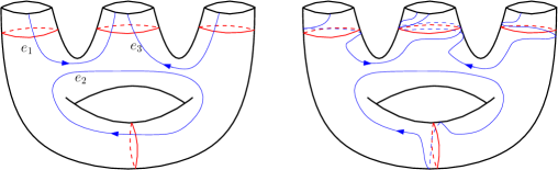
Figure 4.7. The Milnor fiber of the fibration induced by $f$: a torus minus $3$ disks. The monodromy consists of the composition of one right-handed Dehn twist around each of the red curves. In blue we see generators of the relative homology.

With respect to the basis $\{e_{1},e_{2},e_{3}\}$ depicted in Figure 4.7 and the screw numbers, we can compute the associated quadratic form:

$$\left(\begin{array}[]{rrr}2&0&1\\ 0&1&0\\ 1&0&2\end{array}\right).$$

In particular we observe that it is not an even quadratic form (compare with 2.8 and 3.12).

References

• [1] V.I. Arnold, S. M. Gusein-Zade, and A.N. Varchenko, Singularities of differentiable maps. Volume 2, Modern Birkhäuser Classics, Birkhäuser/Springer, New York, 2012.
• [2] D. Corey, J. Ellenberg, and W. Li, The Ceresa class: tropical, topological, and algebraic, 2020, arXiv:2009.10824.
• [3] M.A. Dela-Rosa, On a lemma of Varchenko and higher bilinear forms induced by Grothendieck duality on the Milnor algebra of an isolated hypersurface singularity, Bull. Braz. Math. Soc. (N.S.) 49 (2018), no. 4, 715–741.
• [4] P. Du Bois and F. Michel, Cobordism of algebraic knots via Seifert forms, Invent. Math. 111 (1993), no. 1, 151–169.
• [5] by same author, The integral Seifert form does not determine the topology of plane curve germs, J. Algebraic Geom. 3 (1994), no. 1, 1–38.
• [6] D. Eisenbud and W.D. Neumann, Three-dimensional link theory and invariants of plane curve singularities, Annals of Mathematics Studies, vol. 110, Princeton University Press, Princeton, NJ, 1985.
• [7] B. Farb and D. Margalit, A primer on mapping class groups, Princeton Mathematical Series, vol. 49, Princeton University Press, Princeton, NJ, 2012.
• [8] L. Giraldo, X. Gómez-Mont, and P. Mardešic̀, Flags in zero dimensional complete intersection algebras and indices of real vector fields, Math. Z. 260 (2008), no. 1, 77–91.
• [9] G.L. Gordon, On a simplicial complex associated to the monodromy, Trans. Amer. Math. Soc. 261 (1980), no. 1, 93–101.
• [10] C. Hertling, Classifying spaces for polarized mixed Hodge structures and for Brieskorn lattices, Compositio Math. 116 (1999), no. 1, 1–37.
• [11] by same author, Frobenius manifolds and moduli spaces for singularities, Cambridge Tracts in Mathematics, vol. 151, Cambridge University Press, Cambridge, 2002.
• [12] by same author, Formes bilinéaires et hermitiennes pour des singularités: un aperçu, Singularités, Inst. Élie Cartan, vol. 18, Univ. Nancy, Nancy, 2005, Updated english translation available at https://arxiv.org/abs/2011.10099, pp. 1–17.
• [13] R. Kaenders, The Seifert form of a plane curve singularity determines its intersection multiplicities, Indag. Math. (N.S.) 7 (1996), no. 2, 185–197.
• [14] Lê D.T., Some remarks on relative monodromy, Real and complex singularities (Proc. Ninth Nordic Summer School/NAVF Sympos. Math., Oslo, 1976), 1977, pp. 397–403.
• [15] W. Li, D. Litt, N. Salter, and P. Srinivasan, Surface bundles and the section conjecture, 2020, arXiv:2010.07331.
• [16] I. Luengo, The $\mu$-constant stratum is not smooth, Invent. Math. 90 (1987), no. 1, 139–152.
• [17] J. Martín-Morales, Semistable reduction of a normal crossing $\mathbb{Q}$-divisor, Ann. Mat. Pura Appl. (4) 195 (2016), no. 5, 1749–1769.
• [18] Y. Matsumoto and J.M. Montesinos, Pseudo-periodic maps and degeneration of Riemann surfaces, Lecture Notes in Mathematics, vol. 2030, Springer, Heidelberg, 2011.
• [19] D. Mumford, The topology of normal singularities of an algebraic surface and a criterion for simplicity, Inst. Hautes Études Sci. Publ. Math. (1961), no. 9, 5–22.
• [20] W.D. Neumann, Invariants of plane curve singularities, Knots, braids and singularities (Plans-sur-Bex, 1982), Monogr. Enseign. Math., vol. 31, Enseignement Math., Geneva, 1983, pp. 223–232.
• [21] A. Pichon, Fibrations sur le cercle et surfaces complexes, Ann. Inst. Fourier (Grenoble) 51 (2001), no. 2, 337–374.
• [22] P. Portilla, Monodromies as tête-à-tête graphs, PhD Thesis. (2018), Available at https://www.icmat.es/Thesis/2018/Tesis_Pablo_Portilla.pdf.
• [23] R. Schrauwen, J.H.M Steenbrink, and J. Stevens, Spectral pairs and the topology of curve singularities, Complex geometry and Lie theory (Sundance, UT, 1989), Proc. Sympos. Pure Math., vol. 53, Amer. Math. Soc., Providence, RI, 1991, pp. 305–328.
• [24] A.N. Varchenko, On the monodromy operator in vanishing cohomology and the multiplication operator by $f$ in the local ring, Dokl. Akad. Nauk SSSR 260 (1981), no. 2, 272–276.
• [25] C.T.C. Wall, Quadratic forms and normal surface singularities, Quadratic forms and their applications (Dublin, 1999), Contemp. Math., vol. 272, Amer. Math. Soc., Providence, RI, 2000, pp. 293–311.
• [26] by same author, Singular points of plane curves, London Mathematical Society Student Texts, vol. 63, Cambridge University Press, Cambridge, 2004.
• [27] C. Weber, On the topology of singularities, Singularities II, Contemp. Math., vol. 475, Amer. Math. Soc., Providence, RI, 2008, pp. 217–251.