November, 2020

Particle Production from Oscillating Scalar Field
and Consistency of Boltzmann Equation

Takeo Moroi and Wen Yin

Department of Physics, University of Tokyo, Tokyo 113-0033, Japan

Boltzmann equation plays important roles in particle cosmology in studying the evolution of distribution functions (also called as occupation numbers) of various particles. For the case of the decay of a scalar condensation $\phi$ into a pair of scalar particles (called $\chi$), we point out that the system may not be well described by the Boltzmann equation when the occupation number of $\chi$ becomes large even in the so-called narrow resonance regime. We study the particle production including the possible enhancement due to a large occupation number of the final state particle, known as the stimulated emission or the parametric resonance. Based on the quantum field theory (QFT), we derive a set of equations which directly govern the evolution of the distribution function of $\chi$. Comparing the results of the QFT calculation and those from the Boltzmann equation, we find non-agreements in some cases. In particular, in the expanding Universe, the occupation number of $\chi$ based on the QFT may differ by many orders of magnitude from that from the Boltzmann equation. We also discuss a possible relation between the evolution equations based on the QFT and the Boltzmann equation.

1 Introduction

Boltzmann equation is widely used as a tool to study the evolution of the momentum distribution of multiple states. The success of the standard cosmology or $\Lambda$CDM essentially relies on the use of the Boltzmann equation in an expanding Universe. In cosmology, however, the stimulated emission or Pauli blocking effect is usually omitted (see, for example, [1, 2]).

Scalar fields may form condensation; examples of such scalar fields include inflaton [3, 4, 5, 6, 7], curvaton [8, 9, 10], axion [11, 12, 13, 14, 15], Affleck-Dine field for the baryogenesis [16], and so on. (Hereafter, such a scalar condensation is called $\phi$.) If $\phi$ can decay into a pair of bosonic particles (called $\chi$) as $\phi\to\chi\chi$, the effects of the stimulated emission can be important since the daughter particles may be enormously populated. In particular, recently, a new mechanism of producing bosonic dark matter from the inflaton decay has been proposed [17], in which a stimulated emission of the bosonic dark matter plays an important role.

Such systems have been studied by employing the Boltzmann equation or in the context of the parametric resonance [18, 19, 20, 21, 22, 23, 2, 24, 25, 26, 27, 28, 29, 30, 31, 32, 33, 34, 35, 36]. In particular, particle production from an oscillating scalar field has been intensively investigated, particularly using the Mathieu equation [37, 38]. In the previous studies, the evolution equation of the expectation value of the field operator (which we call wave function) for the final-state particle is converted to the Mathieu equation, based on which the occupation number of the final state particle has been estimated. Then, it has been shown that there exist resonance bands and that the occupation numbers in the resonance bands grow exponentially. In the broad resonance region, it has been known that the particle production is non-perturbative and that the process cannot be described by the Boltzmann equation. On the contrary, sometimes it has been argued that the Boltzmann equation can provide a proper description in the narrow resonance regime.

In this paper, we study the particle production from an oscillating scalar field in the narrow resonance regime. We pay particular attention to the relation between the results based on the Boltzmann equation and those from the quantum field theory (QFT). Even though the effects of the stimulated emission may be included in the Boltzmann equation [1, 2], it is unclear whether the Boltzmann equation can properly describe the particle production from the oscillating scalar field from the QFT point of view, in particular, the parametric resonance. Based on the QFT, we derive a set of equations which directly govern the evolution of the occupation number of the final state particle $\chi$ with an oscillating $\phi$ background. We will see that the results of our evolution equations are in good agreement with those from the conventional approach with the Mathieu equation. Then, we compare the occupation number obtained from the QFT calculation with that from the Boltzmann equation. We will see that the results from the QFT and the Boltzmann equation may differ even in the narrow resonance regime when the occupation number becomes larger than $\sim 1$. In particular, in the expanding Universe, growth factors derived from two approaches may differ many orders of magnitude. We also discuss how our evolution equations can be related to the conventional Boltzmann equation and consider a possible explanation of the discrepancy.

This paper is organized as follows. In Section 2, the setup of our analysis is given. In Section 3, we derive the evolution equations and discuss particle production in the flat spacetime. In Section 4, we study particle production taking into account the cosmic expansion. Section 5 is devoted to the summary of this paper.

2 Setup

Here, we study particle production from an oscillating real scalar field $\phi$, whose mass is $m_{\phi}$. We concentrate on the case that $\phi$ is spatially homogeneous and the scalar field $\phi$ depends only on time $t$. We consider the timescale much shorter than the dissipation of the motion of $\phi$ and the back reaction. Then, assuming that the potential of $\phi$ is well approximated by a parabolic one, the motion of $\phi$ is described as

$$\phi(t)=\bar{\phi}\cos m_{\phi}t,$$ (2.1)

where $\bar{\phi}$ is the amplitude. The number density of $\phi$ is given by

$$n_{\phi}=\frac{1}{2}m_{\phi}\bar{\phi}^{2}.$$ (2.2)

The scalar field $\phi$ is assumed to interact with a real scalar field $\chi$. Although our discussion holds as far as the interaction Hamiltonian has the form of Eq. (3.5) given below, we consider the following interaction Hamiltonian to make our discussion concrete:

$$H_{\rm int}=A\int d^{3}x\phi\chi^{2},$$ (2.3)

where $A$ is a dimension 1 coupling constant. With the above interaction Hamiltonian, the decay rate for the process of $\phi\rightarrow\chi\chi$ is obtained as

$$\Gamma_{\phi\rightarrow\chi\chi}^{(0)}=\frac{A^{2}}{8\pi m_{\phi}}\frac{2p_{\chi}}{m_{\phi}},$$ (2.4)

where $p_{\chi}$ is the three-momentum of $\chi$ produced by the decay:

$$p_{\chi}\equiv\frac{1}{2}m_{\phi}\sqrt{1-\frac{4m_{\chi}^{2}}{m_{\phi}^{2}}},$$ (2.5)

with $m_{\chi}$ being the mass of $\chi$. In Eq. (2.4), the superscript “(0)” indicates that $\Gamma_{\phi\rightarrow\chi\chi}^{(0)}$ is the perturbative decay rate in the vacuum.

The production of $\chi$ in the system introduced above has been also studied in the context of parametric (or tachyonic) resonance [19, 23, 24, 29]. In particle production through the parametric resonance, the modes in resonance bands are effectively produced. In the present case, the widths of the bands are determined by the following parameter:

$$q\equiv\frac{4A\bar{\phi}}{m_{\phi}^{2}}.$$ (2.6)

As we will see below, the band width is $\sim qm_{\phi}$. Hereafter, for the comparison with the Boltzmann equation, we concentrate on the case that the band widths are narrow, i.e.,

$$q\ll 1.$$ (2.7)

In the narrow resonance regime, $\chi$ is produced almost “on-resonance,” i.e., the momentum of $\chi$ produced from the $\phi$ oscillation is $|\vec{k}|\simeq p_{\chi}$. In the perturbative description, effects which are higher order in $A$ are suppressed when $q$ is small [25].

3 Particle Production in Flat Spacetime

3.1 Evolution equations from QFT

In studying particle production in the QFT, an approach by employing the Mathieu equation has been often used in the context of parametric resonance. In our analysis, however, we adopt a different approach, which should be equivalent to the one with the Mathieu equation, by deriving evolution equations for the distribution function. An advantage of our approach is that the equations directly describe the evolution of the distribution function. Because of this, we can consider a possible relation between the evolution equation of the distribution function in the QFT and the Boltzmann equation.

We first discuss particle production in the flat (i.e., Minkowski) spacetime. We decompose $\chi$ by using the creation and annihilation operators, denoted as $a_{\vec{k}}$ and $a^{\dagger}_{\vec{k}}$, respectively:

$$\chi(x)=\int{\frac{d^{3}k}{(2\pi)^{3}\sqrt{2\omega_{k}}}}\left[e^{i\vec{k}\vec{x}}a_{\vec{k}}(t)+e^{-i\vec{k}\vec{x}}a^{\dagger}_{\vec{k}}(t)\right].$$ (3.1)

The creation and annihilation operators satisfy the following commutation relation:

$$[a_{\vec{k}},a^{\dagger}_{\vec{k^{\prime}}}]=(2\pi)^{3}\delta^{(3)}(\vec{k}-\vec{k^{\prime}}).$$ (3.2)

With the creation and annihilation operators, the free part of the Hamiltonian is given by

$$H_{\rm free}=\int\frac{d^{3}k}{(2\pi)^{3}}\omega_{{k}}a_{\vec{k}}^{\dagger}a_{\vec{k}},$$ (3.3)

where

$$\omega_{k}\equiv\sqrt{|\vec{k}|^{2}+m_{\chi}^{2}}.$$ (3.4)

In addition, the interaction Hamiltonian is expressed as

$$H_{\rm int}(t)=A\phi(t)\int\frac{d^{3}k}{(2\pi)^{3}2\omega_{{k}}}\left[a^{\dagger}_{\vec{k}}(t)a_{\vec{k}}(t)+a_{\vec{k}}(t)a^{\dagger}_{\vec{k}}(t)+a_{\vec{k}}(t)a_{-\vec{k}}(t)+a^{\dagger}_{\vec{k}}(t)a^{\dagger}_{-\vec{k}}(t)\right].$$ (3.5)

In order to study the production of $\chi$, we introduce the distribution function of $\chi$:

$$f_{\vec{k}}(t)\equiv\frac{1}{V}\langle a_{\vec{k}}^{\dagger}(t)a_{\vec{k}}(t)\rangle,$$ (3.6)

where $V$ is the spatial volume, and the expectation value of the operator ${\mathcal{O}}$ is defined by using a density matrix $\rho$ as

$$\langle{\mathcal{O}}\rangle\equiv\mbox{Tr}(\rho{\mathcal{O}}).$$ (3.7)

Using the distribution function, the number density of $\chi$ is given by

$$n_{\chi}(t)=\int\frac{d^{3}k}{(2\pi)^{3}}f_{\vec{k}}(t).$$ (3.8)

In the following, we work in the interaction picture. The time dependence of the operator $\mathcal{O}$ is given by

$$\dot{\mathcal{O}}=-i[\mathcal{O},H_{\rm free}],$$ (3.9)

where the “dot” denotes the derivative with respect to time, and hence

$$\dot{a}_{\vec{k}}=-i\omega_{k}a_{\vec{k}}.$$ (3.10)

In addition, the density matrix evolves as

$$\dot{\rho}=i[\rho,H_{\rm int}].$$ (3.11)

Consequently, the evolution of the expectation value of the operator $\mathcal{O}$ is governed by the following differential equation:

$$\frac{d}{dt}\langle\mathcal{O}\rangle=-i\langle[\mathcal{O},H_{\rm int}]\rangle+\langle\dot{\mathcal{O}}\rangle.$$ (3.12)

In order to study the evolution of the distribution function, we also introduce

$$g_{\vec{k}}\equiv\frac{1}{V}\langle a_{\vec{k}}a_{-\vec{k}}\rangle.$$ (3.13)

Then, the time derivatives of $f_{\vec{k}}$ and $g_{\vec{k}}$ are given by

$$\dot{f}_{\vec{k}}= \,i\frac{A\bar{\phi}}{\omega_{k}}\left(g_{\vec{k}}-g_{\vec{k}}^{*}\right)\cos m_{\phi}t,$$ (3.14)

$$\dot{g}_{\vec{k}}= \,-i\left[2\omega_{k}g_{\vec{k}}+\frac{A\bar{\phi}}{\omega_{k}}\left(1+f_{\vec{k}}+f_{-\vec{k}}+2g_{\vec{k}}\right)\cos m_{\phi}t\right].$$ (3.15)

We consider isotropic solutions, and the momentum dependences of $f_{\vec{k}}$ and $g_{\vec{k}}$ are only via $k\equiv|\vec{k}|$; thus, in the following, these functions are denoted as $f_{k}$ and $g_{k}$, respectively. We decompose the complex function $g_{k}$ as

$$g_{k}(t)=e^{-2i\omega_{k}t}\left[\xi_{k}(t)+i\eta_{k}(t)\right],$$ (3.16)

where $\xi_{k}$ and $\eta_{k}$ are real functions. Then, the evolution equations become

$$\dot{f}_{k}= \,\frac{A\bar{\phi}}{\omega_{k}}\cos m_{\phi}t\left[2\xi_{k}\sin 2\omega_{k}t-2\eta_{k}\cos 2\omega_{k}t\right],$$ (3.17)

$$\dot{\xi}_{k}= \,\frac{A\bar{\phi}}{\omega_{k}}\cos m_{\phi}t\left[(1+2f_{k})\sin 2\omega_{k}t+\eta_{k}\right],$$ (3.18)

$$\dot{\eta}_{k}= \,\frac{A\bar{\phi}}{\omega_{k}}\cos m_{\phi}t\left[-(1+2f_{k})\cos 2\omega_{k}t-\xi_{k}\right].$$ (3.19)

We note that the evolution equations above also apply to the case of $q\gtrsim 1$, although we do not consider such a case in this paper.

Before solving these differential equations, we comment on the initial condition. Because we study the $\chi$ production from the $\phi$ oscillation, we consider the case that the $\chi$ sector is initially at the ground state (vacuum), denoted as $|0\rangle$; thus, $\rho(0)=|0\rangle\langle 0|$. Because $a_{k}|0\rangle=\langle 0|a_{k}^{\dagger}=0$, $f_{k}$ and $g_{k}$ should satisfy

$$f_{k}(0)=\xi_{k}(0)=\eta_{k}(0)=0.$$ (3.20)

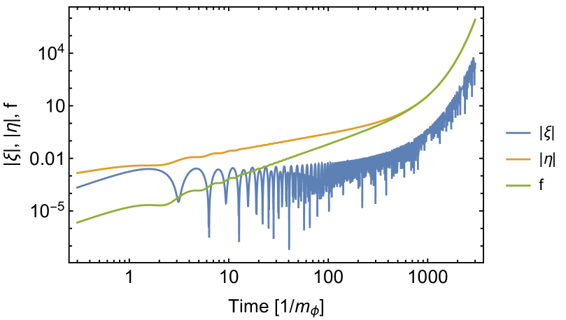
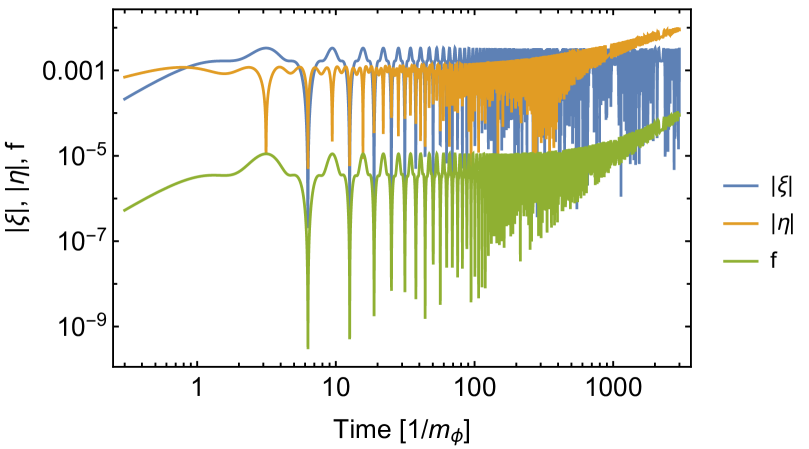
Figure 1: $|\xi_{k}|$ (blue), $|\eta_{k}|$ (orange), and $f_{k}$ (green), as functions of time (in units of $m_{\phi}^{-1}$). Here, we take $q=10^{-2}$, and $\omega=\frac{1}{2}m_{\phi}$.

Figure 2: Same as Fig. 2, except for $\omega=m_{\phi}$.

We numerically solve Eqs. (3.17) $-$ (3.19) with the initial condition given by Eq. (3.20). The evolutions for $\omega_{k}=\frac{1}{2}m_{\phi}$ and $m_{\phi}$ are shown in Figs. 2 and 2, respectively, with taking $q=10^{-2}$. As one can see, $f_{k}$ monotonically increases when $t\lesssim m_{\phi}$ irrespective of $\omega_{k}$ (as far as $\omega_{k}\lesssim m_{\phi}$). The behavior at $t\rightarrow\infty$ strongly depends on $\omega_{k}$. For $\omega_{k}=\frac{1}{2}m_{\phi}$, the functions $f_{k}$ and $\eta_{k}$ grow exponentially at $t\rightarrow\infty$, while $\xi_{k}$ is oscillating. On the contrary, for $\omega=m_{\phi}$, $f_{k}$ does not show the growing behavior at $t\rightarrow\infty$.

The behaviors of $f_{k}$, $\xi_{k}$, and $\eta_{k}$ at $t\ll m_{\phi}$ can be obtained by expanding these functions as a power series of $t$. With $t$ being small enough, the effects of the oscillation of $\phi$ is unimportant and we obtain

$$\left.f_{k}(t)\right|_{t\ll m_{\phi}^{-1}}\simeq \,\frac{1}{4}q^{2}m_{\phi}^{2}t^{2},$$ (3.21)

$$\left.\xi_{k}(t)\right|_{t\ll m_{\phi}^{-1}}\simeq \,\frac{1}{4}qm_{\phi}^{2}t^{2},$$ (3.22)

$$\left.\eta_{k}(t)\right|_{t\ll m_{\phi}^{-1}}\simeq \,-\frac{1}{2}qm_{\phi}t.$$ (3.23)

We can also understand the exponential growths of the modes with $\omega_{k}\sim\frac{1}{2}m_{\phi}$ at $t\rightarrow\infty$. We first adopt the following ansatz:

$$\left.f_{k}(t)\right|_{t\gtrsim(qm_{\phi})^{-1}}\simeq\alpha_{k}e^{\lambda_{k}t},$$ (3.24)

where $\alpha_{k}$ and $\lambda_{k}$ are positive constants. Substituting the above ansatz, Eq. (3.15) becomes

$$g_{k}(t)\simeq\frac{2A\bar{\phi}}{\omega_{k}}\frac{1}{m_{\phi}^{2}-(2\omega_{k}-i\lambda_{k})^{2}}\left[(2\omega_{k}-i\lambda_{k})\cos m_{\phi}t-im_{\phi}\sin m_{\phi}t\right]f_{k}(t),$$ (3.25)

where we neglect terms which are not exponentially growing, and

$$\mbox{Im}g_{k}(t)\simeq \,-\frac{A\bar{\phi}}{\omega_{k}}\frac{1}{(2\omega_{k}-m_{\phi})^{2}+\lambda_{k}^{2}}\left[\lambda_{k}\cos m_{\phi}t-(2\omega_{k}-m_{\phi})\sin m_{\phi}t\right]f_{k}(t)$$

$$\,-\frac{A\bar{\phi}}{\omega_{k}}\frac{1}{(2\omega_{k}+m_{\phi})^{2}+\lambda_{k}^{2}}\left[\lambda_{k}\cos m_{\phi}t+(2\omega_{k}+m_{\phi})\sin m_{\phi}t\right]f_{k}(t).$$ (3.26)

For the study of the modes with $\omega_{k}\sim\frac{1}{2}m_{\phi}$, we neglect the second term of the right-hand side of the above equation because it is sub-dominant. Combining Eqs. (3.14) and (3.26), we obtain

$$\frac{\dot{f}_{k}}{f_{k}}\simeq 2\left(\frac{A\bar{\phi}}{\omega_{k}}\right)^{2}\frac{1}{(2\omega_{k}-m_{\phi})^{2}+\lambda_{k}^{2}}\cos m_{\phi}t\left[\lambda_{k}\cos m_{\phi}t-(2\omega_{k}-m_{\phi})\sin m_{\phi}t\right].$$ (3.27)

We neglect terms which are oscillating with the timescale of $\sim m_{\phi}^{-1}$ because we are not interested in terms with rapid oscillations. We define the time average of the function $F(t)$ as

$$\langle F\rangle_{t}\equiv\frac{1}{t_{*}}\int_{t}^{t+t_{*}}dt^{\prime}F(t^{\prime}),$$ (3.28)

where the timescale $t_{*}$ is taken to be $m_{\phi}^{-1}\ll t_{*}\ll(qm_{\phi})^{-1}$. Using the relation $\langle\cos^{2}m_{\phi}t\rangle_{t}\simeq\frac{1}{2}$ and $\langle\sin 2m_{\phi}t\rangle_{t}\simeq 0$, we can see that Eqs. (3.14) and (3.15) are satisfied with the ansatz given in Eq. (3.24) (neglecting rapidly oscillating terms and terms which do not grow exponentially) if

$$\lambda_{k}=\sqrt{\frac{1}{4}\left(\frac{m_{\phi}}{2\omega_{k}}\right)^{2}q^{2}m_{\phi}^{2}-(2\omega_{k}-m_{\phi})^{2}}.$$ (3.29)

The growth rate $\lambda_{k}$ should be real, which determines the resonance band. We can see that the width of the resonance band is of $O(qm_{\phi})$. Then, keeping the leading term in $q$, we may use

$$\lambda_{k}\simeq\sqrt{\frac{1}{4}q^{2}m_{\phi}^{2}-(2\omega_{k}-m_{\phi})^{2}},$$ (3.30)

and the resonance band is given by $\omega_{-}\lesssim\omega_{k}\lesssim\omega_{+}$, where

$$\omega_{\pm}\equiv\frac{1}{2}m_{\phi}\left(1\pm\frac{1}{2}q\right).$$ (3.31)

Notice that the resonance band given above corresponds to the first resonance band in the study of the parametric resonance, and that the growth rate given in Eq. (3.30) is consistent with that given in [21, 23, 24].

$z$	Numerical	Eq. (3.24)
$-0.4$	$7.3\times 10^{11}$	$6.2\times 10^{11}$
$-0.2$	$8.9\times 10^{17}$	$8.6\times 10^{17}$
$0$	$3.5\times 10^{19}$	$3.5\times 10^{19}$
$0.2$	$7.7\times 10^{17}$	$7.8\times 10^{17}$
$0.4$	$4.7\times 10^{11}$	$4.6\times 10^{11}$

Table 1: The ratio $f_{k}(t=100(qm_{\phi})^{-1})/f_{k}(t=10(qm_{\phi})^{-1})$, based on the numerical calculation (Numerical) and the approximation adopting the ansatz of the exponential increase (Eq. (3.24)) with the growth rate given in Eq. (3.29). We take $q=10^{-2}$, and several values of $\omega_{k}$ (parameterized as $\omega_{k}=\frac{1}{2}m_{\phi}(1+zq)$).

In order to check the validity of the ansatz of the exponential increase given in Eq. (3.24), we compare the value of $f_{k}(t=100(qm_{\phi})^{-1})/f_{k}(t=10(qm_{\phi})^{-1})$ obtained from the numerical calculation and that predicted by Eq. (3.24) (with the growth rate given in Eq. (3.29)). The results with taking $q=10^{-2}$ are shown in Table 1 for several values of $\omega_{k}$ in the resonance band. Notice that $f_{k}(t=10(qm_{\phi})^{-1})$ is of $O(10)$ for the frequencies considered in Table 1, and hence the effect of stimulated emission is already important when $t=10(qm_{\phi})^{-1}$. We can see that the occupation number in the resonance band is well described by the exponential increase with the growth rate given above once the effect of the stimulated emission becomes effective.

3.2 QFT and ordinary Boltzmann equation

The relation between the analysis so far and that based on the conventional Boltzmann equation is interesting. Sometimes particle production from the oscillating scalar field $\phi$ is studied by using Boltzmann equation. $\phi$ can be regarded as a coherent state of a non-relativistic scalar field and the production of $\chi$ may be regarded as the decay of $\phi$. Then, the collision term in the Boltzmann equation is given by (see, for example, [1, 2])

$$\dot{f}_{k}^{\rm(coll)}(t)=\frac{4\pi^{2}n_{\phi}\Gamma_{\phi\rightarrow\chi\chi}^{(0)}}{p_{\chi}^{2}}\left[(1+f_{k})^{2}-f_{k}^{2}\right]\delta(k-p_{\chi}),$$ (3.32)

where the first and the second terms in the square bracket describe the effects of the decay and the inverse decay of $\phi$, respectively. In the following, we consider how the collision term can be related to the argument based on the QFT. We treat the cases of $t\lesssim(qm_{\phi})^{-1}$ and $t\gtrsim(qm_{\phi})^{-1}$ separately.

When $t\lesssim(qm_{\phi})^{-1}$, $f_{k}$ is smaller than $1$ and the solution of Eq. (3.15) is approximately given by

$$g_{k}(t)\simeq-\frac{1}{4\omega_{k}^{2}-m_{\phi}^{2}}\frac{A\bar{\phi}}{\omega_{k}}\left(-2c\omega_{k}e^{-2i\omega_{k}t}+2\omega_{k}\cos m_{\phi}t-im_{\phi}\sin m_{\phi}t\right),$$ (3.33)

where $c$ is a constant. Here, we have neglected the last term of the right-hand side of Eq. (3.15) because it is of $O(q)$ and is sub-dominant relative to the first term. Because $g_{k}(0)=0$ and also because $g_{k}$ is non-singular at $\omega_{k}\rightarrow\frac{1}{2}m_{\phi}$, $c=1$ and hence $\dot{f}_{k}$ becomes

$$\left.\dot{f}_{k}\right|_{t\lesssim(qm_{\phi})^{-1}}\simeq\frac{\pi}{4}\left(\frac{A\bar{\phi}}{\omega_{k}}\right)^{2}\gamma(\omega_{k};t),$$ (3.34)

where

$$\gamma(\omega;t)\equiv\frac{8}{\pi(4\omega^{2}-m_{\phi}^{2})}\cos m_{\phi}t\left(2\omega\sin 2\omega t-m_{\phi}\sin m_{\phi}t\right).$$ (3.35)

In the above expression, we neglect the terms which are rapidly oscillating with the timescale of $\sim m_{\phi}^{-1}$ (even in the limit of $\omega_{k}\rightarrow\frac{1}{2}m_{\phi}$). Notice that the function $\gamma(\omega;t)$ has the following property:

$$\int_{0}^{\infty}d\omega\gamma(\omega;t)=1+\cos 2m_{\phi}t.$$ (3.36)

We consider the time averaged value of $\dot{f}_{k}$ and neglect terms which are rapidly oscillating:

$$\left.\langle\dot{f}_{k}\rangle_{t}\right|_{t\lesssim(qm_{\phi})^{-1}}\simeq\frac{\pi}{4}\left(\frac{A\bar{\phi}}{\omega_{k}}\right)^{2}\Delta(\omega_{k};t_{*}),$$ (3.37)

where

$$\Delta(\omega;t_{*})\equiv\frac{1}{t_{*}}\int_{0}^{t_{*}}dt\gamma(\omega;t).$$ (3.38)

Using Eq. (3.36), we obtain

$$\lim_{t_{*}\rightarrow\infty}\int_{0}^{\infty}d\omega\Delta(\omega;t_{*})=\lim_{t_{*}\rightarrow\infty}\frac{1}{t_{*}}\int_{t}^{t+t_{*}}dt^{\prime}\left(1+\cos 2m_{\phi}t^{\prime}\right)=1.$$ (3.39)

In addition,

$$\left.\lim_{t_{*}\rightarrow\infty}\Delta(\omega;t_{*})\right|_{2|\omega|\neq m_{\phi}}=0.$$ (3.40)

Thus, assuming that $t_{*}$ can be chosen to be large enough, we may approximate

$$\Delta(\omega;t_{*})\rightarrow\delta(\omega-\mbox{$\frac{1}{2}$}m_{\phi}),$$ (3.41)

and obtain

$$\left.\langle\dot{f}_{k}\rangle_{t}\right|_{t\lesssim(qm_{\phi})^{-1}}\simeq\frac{4\pi^{2}n_{\phi}\Gamma_{\phi\rightarrow\chi\chi}^{(0)}}{p_{\chi}^{2}}\delta(k-p_{\chi}).$$ (3.42)

When $t\gtrsim(qm_{\phi})^{-1}$, $f_{k}$ in the resonance band shows the exponential growth and is much larger than $1$, while $g_{k}$ behaves as Eq. (3.25). In such a case, the conventional Boltzmann equation is obtained if one performs the following replacement in Eq. (3.25):

$$\frac{1}{m_{\phi}^{2}-(2\omega_{k}-i\lambda_{k})^{2}}\rightarrow-i\frac{\pi}{2m_{\phi}}\delta(2\omega_{k}-m_{\phi})+(\mbox{irrelevant}).$$ (3.43)

Here, the relation $\frac{1}{x-i0}=P(\frac{1}{x})+i\pi\delta(x)$ (with $P$ being the principal value), as well as the smallness of $\lambda_{k}$ relative to $m_{\phi}$, are used. However, we should note that this replacement is allowed if $\lambda_{k}$ does not depend much on $\omega_{k}$ and also if $f_{k}(t)$ is insensitive to $k$ around the pole. These requirements may not be satisfied in the case of our interest (see Eq. (3.30)), which may result in the non-agreements between the result of the QFT calculation and that of the Boltzmann equation. Substituting Eq. (3.25) (with using the above replacement) into Eq. (3.14), we obtain

$$\left.\dot{f}_{k}\right|_{t\gtrsim(qm_{\phi})^{-1}}\simeq 8\pi\left(\frac{A\bar{\phi}}{m_{\phi}}\right)^{2}\cos^{2}m_{\phi}tf_{k}(t)\delta(2\omega_{k}-m_{\phi}).$$ (3.44)

Neglecting the rapidly oscillating term with taking the time average,

$$\left.\langle\dot{f}_{k}\rangle_{t}\right|_{t\gtrsim(qm_{\phi})^{-1}}\simeq\frac{8\pi^{2}n_{\phi}\Gamma_{\phi\rightarrow\chi\chi}^{(0)}}{p_{\chi}^{2}}f_{k}(t)\delta(k-p_{\chi}).$$ (3.45)

Combining the results for $t\lesssim(qm_{\phi})^{-1}$ and $t\gtrsim(qm_{\phi})^{-1}$, which are given in Eqs. (3.42) and (3.45), respectively, and estimating the collision term as

$$\dot{f}_{k}^{\rm(coll)}(t)\simeq\langle\dot{f}_{k}(k)\rangle_{t},$$ (3.46)

we find that the collision term given in (3.32) well describes the evolution of $f_{k}$ if the assumptions and approximations adopted in the above argument are valid.

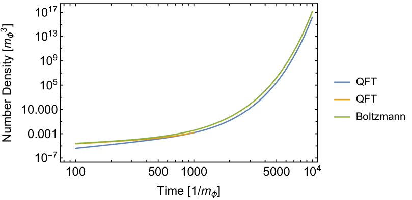
Figure 3: Evolution of $n_{\chi}^{\rm(QFT)}$ (in units of $m_{\phi}^{3}$) for $q=10^{-2}$, adopting the integration regions of $|\omega-\frac{1}{2}m_{\phi}|\leq\frac{1}{4}qm_{\phi}$ and $\frac{5}{2}qm_{\phi}$ (blue and orange, respectively). We also show the evolution of $n_{\chi}^{\rm(Boltzmann)}$ (green).

In order to see the validity of the collision term from the QFT point of view, we calculate the number density of $\chi$ with two different methods, taking $m_{\chi}=0$ (and hence $\omega_{k}=k$) and $q=10^{-2}$.

• First, we use the QFT approach; the number density based on the QFT is denoted as $n_{\chi}^{\rm(QFT)}$. Eq. (3.8) gives

  $$n_{\chi}^{\rm(QFT)}(t)=\frac{1}{2\pi^{2}}\int dkk^{2}f_{k}(t).$$ (3.47)

  When $t\gtrsim(qm_{\phi})^{-1}$, $f_{k}(t)$ is sharply peaked at $k\sim\frac{1}{2}m_{\phi}$, and $n_{\chi}^{\rm(QFT)}$ is insensitive to the integration region. Here, unless otherwise mentioned, we choose the integration region to be within the resonance band: $|k-\frac{1}{2}m_{\phi}|\leq\frac{1}{4}qm_{\phi}$.

• Second, we use the Boltzmann equation; the number density based on the Boltzmann equation is denoted as $n_{\chi}^{\rm(Boltzmann)}$. Solving $\dot{f}_{k}=\dot{f}_{k}^{\rm(coll)}$, we obtain

  $$n_{\chi}^{\rm(Boltzmann)}(t)=2\Gamma_{\phi}^{(0)}n_{\phi}\int_{0}^{t}dt^{\prime}\left(1+2f_{p_{\chi}}(t^{\prime})\right).$$ (3.48)

  Notice that, in the above expression, the distribution function in the parenthesis is that for $k=p_{\chi}$ and is obtained by solving Eqs. (3.14) and (3.15).

The time dependences of $n_{\chi}^{\rm(QFT)}$ and $n_{\chi}^{\rm(Boltzmann)}$ are shown in Fig. 3. We find that the behaviors of $n_{\chi}^{\rm(QFT)}$ and $n_{\chi}^{\rm(Boltzmann)}$ are similar, although $n_{\chi}^{\rm(QFT)}(t)$ is smaller. For $t\sim(qm_{\phi})^{-1}$, the width of the peak of $f_{k}$ around $k=\frac{1}{2}m_{\phi}$ is significantly larger than $\frac{1}{4}qm_{\phi}$, and hence $n_{\chi}^{\rm(QFT)}(t)$ underestimates the number density with our choice of the integration region. If we expand the integration region as $|k-\frac{1}{2}m_{\phi}|\leq\frac{5}{2}qm_{\phi}$, for example, the agreement for $t\sim(qm_{\phi})^{-1}$ becomes much better; difference between $n_{\chi}^{\rm(QFT)}$ and $n_{\chi}^{\rm(Boltzmann)}$ is $\sim 10\ \%$ with such a choice of the integration region. In Fig. 3, we also show $n_{\chi}^{\rm(QFT)}$ with adopting the integration region of $|k-\frac{1}{2}m_{\phi}|\leq\frac{5}{2}qm_{\phi}$. (We show such a result only for relatively small $t$ because the calculation of $n_{\chi}^{\rm(QFT)}$ with larger $t$ requires a computational cost.) For $t\gg(qm_{\phi})^{-1}$, on the contrary, the peak width of $f_{k}$ is smaller than the width of the resonance band (see below). For the replacement given in Eq. (3.43), it is required that the function $f_{k}$ is well approximated by $f_{p_{\chi}}$ for $|k-\frac{1}{2}m_{\phi}|\lesssim\lambda_{k}$ and that the $\omega_{k}$ dependence of $\lambda_{k}$ is unimportant. These cannot be the case in particular when $t\gg(qm_{\phi})^{-1}$. Consequently, $n_{\chi}^{\rm(Boltzmann)}$ becomes larger than $n_{\chi}^{\rm(QFT)}$, as shown in Fig. 3.

We can understand the asymptotic behaviors of $n_{\chi}^{\rm(QFT)}$ and $n_{\chi}^{\rm(Boltzmann)}$ for $t\gg(qm_{\phi})^{-1}$ as follows. At $t\gg(qm_{\phi})^{-1}$, as we see below, $f_{k}$ is sharply peaked at $\omega_{k}=\frac{1}{2}m_{\phi}$. We expand $\lambda_{k}$ around the peak and obtain

$$f_{k}(t)\simeq\alpha_{k}e^{\frac{qm_{\phi}t}{2}}e^{-\frac{(2\omega_{k}-m_{\phi})^{2}}{qm_{\phi}/t}}.$$ (3.49)

Because of the second exponential factor, the width of $f_{k}(t)$ gets smaller as $t$ increases. By using the above expression with neglecting $m_{\chi}$, $n_{\chi}^{\rm(QFT)}(t)$ at $t\gg(qm_{\phi})^{-1}$ is estimated as

$$n_{\chi}^{\rm(QFT)}(t)\sim\frac{1}{16\pi}(\pi qm_{\phi}t)^{-1/2}qm_{\phi}^{3}f_{p_{\chi}}.$$ (3.50)

We can see that the above expression is in a good agreement with the numerical result. In addition,

$$n_{\chi}^{\rm(Boltzmann)}(t)\sim\frac{1}{32\pi}qm_{\phi}^{3}f_{p_{\chi}}.$$ (3.51)

Thus, when $t\gg(qm_{\phi})^{-1}$, $n_{\chi}^{\rm(Boltzmann)}(t)$ becomes larger than $n_{\chi}^{\rm(QFT)}(t)$.

One may wonder if we can introduce an “averaged” occupation number (or growth rate) in the resonance band to make two approaches consistent. However, as we will see in the next section, the discrepancy in the case with the cosmic expansion cannot be solved with such a prescription. (In addition, in Appendix A, we give a consideration about the relation between the QFT and Boltzmann equation.)

Before closing this section, we comment on the back reaction. In our analysis, the effects of the back reaction are neglected; we assume that the amplitude of the $\phi$ oscillation does not depend on time and that the motion of $\phi$ is well described by Eq. (2.1). This is the case when the energy density transferred to the $\chi$ sector is smaller than the initial energy density in the $\phi$ sector. Let us denote the typical value of the occupation number of the modes in the resonance band as $f^{\rm(res)}$; conservatively, we may take $f^{\rm(res)}\sim f_{k=p_{\chi}}$. Then, by using the fact that the width of the resonance band is $\sim qm_{\phi}$, the energy density in the $\chi$ sector is estimated as $\rho_{\chi}\sim f^{\rm(res)}qm_{\phi}^{4}$. Requiring that $\rho_{\chi}$ is smaller than the initial energy density of $\phi$, we obtain

$$f^{\rm(res)}qm_{\phi}^{2}\ll\bar{\phi}^{2},$$ (3.52)

and, equivalently, $f^{\rm(res)}A\ll\bar{\phi}$. The above constraint can be satisfied for any value of $q$ by taking large enough $\bar{\phi}$ (and small enough $A$). Our results are applicable to the parameter region consistent with the above constraint. We may also define the effective decay rate $\Gamma_{\phi\rightarrow\chi\chi}^{\rm(eff)}$ as the inverse of the timescale with which a single $\phi$ becomes a pair of $\chi$; we can estimate $\Gamma_{\phi\rightarrow\chi\chi}^{\rm(eff)}\sim f^{\rm(res)}\Gamma_{\phi\rightarrow\chi\chi}^{(0)}$. With the constraint (3.52) being satisfied, $\Gamma_{\phi\rightarrow\chi\chi}^{\rm(eff)}$ is always smaller than $qm_{\phi}$ as far as $q\ll 1$. Another back reaction may be due to the scattering process like $\chi\phi\rightarrow\chi\phi$ (with $\phi$ in the initial state being that in the coherent oscillation). Such a scattering process may remove $\chi$ from the resonance band. Effects of the scattering processes are not taken into account in our analysis because $\phi$ is treated as a classical field. One can estimate the interaction rate as $\Gamma^{(\rm scat)}\sim q^{4}\frac{m_{\phi}^{3}}{\bar{\phi}^{2}}$ which can be neglected compared with the growth rate which is of $O(qm_{\phi})$.

4 Particle Production with Cosmic Expansion

In this section, we study particle production taking into account the effects of the cosmic expansion. We show that the analysis based on the Boltzmann equation may result in a significant overestimation of the occupation number of $\chi$ compared to the analysis based on the QFT.

4.1 Particle production with cosmic expansion from QFT

With the cosmic expansion, the momentum of each mode redshifts. Thus, if we consider a mode which has a frequency larger than $\omega_{+}$ in an early epoch, it enters the resonance band as the Universe expands, then the frequency becomes smaller than $\omega_{-}$ and the mode exits the resonance band. The occupation number may exponentially increase when the mode is in the resonance band, as we see below.

Here, we are particularly interested in the behavior of the occupation number when the mode is around the resonance band. The timescale of the mode to go through the resonance band is $\sim qH^{-1}$, where $H$ is the expansion rate:

$$H\equiv\frac{\dot{a}}{a},$$ (4.1)

with $a$ being the scale factor. The timescale of the evolution of the occupation number is much shorter than the timescale of the cosmic expansion because $q\ll 1$ and hence the change of $H$ is unimportant. In the following analysis, we neglect the time dependence of $H$ and take

$$a(t)=a_{0}e^{Ht},$$ (4.2)

with $a_{0}$ being a constant. Due to the same reason, again we treat $\bar{\phi}$ as constant.

Because of the hierarchy between the timescales of the cosmic expansion and the evolutions of $f_{k}$ and $g_{k}$, for the timescale shorter than $H^{-1}$, evolutions of $f_{k}$ and $g_{k}$ are expected to be the same as those in the flat spacetime. Then, $f_{k}$ and $g_{k}$ obey

$$\dot{f}_{k}= \,kH\frac{\partial f_{k}}{\partial k}+i\frac{A\bar{\phi}}{\omega_{k}}\left(g_{k}-g_{k}^{*}\right)\cos m_{\phi}t,$$ (4.3)

$$\dot{g}_{k}= \,kH\frac{\partial g_{k}}{\partial k}-i\left[2\omega_{k}g_{k}+\frac{A\bar{\phi}}{\omega_{k}}\left(1+2f_{k}+2g_{k}\right)\cos m_{\phi}t\right],$$ (4.4)

where the first terms of the right-hand sides of the above equations describe the effect of redshift. We can simplify solve the above equations by introducing functions for a fixed comoving momentum:

$$f_{\star}(t)\equiv f_{k=K(t)}(t),~{}~{}~{}g_{\star}(t)\equiv g_{k=K(t)}(t),$$ (4.5)

where $K(t)$ is the physical momentum for the given comoving momentum $\hat{k}$ (which is independent of time):

$$K(t)\equiv\frac{a_{0}}{a(t)}\hat{k}.$$ (4.6)

We decompose the function $g_{\star}$ using real functions $\xi_{\star}$ and $\eta_{\star}$ as

$$g_{\star}(t)=e^{-2i\Theta(t)}\left[\xi_{\star}(t)+i\eta_{\star}(t)\right],$$ (4.7)

where

$$\Theta(t)\equiv\int^{t}dt^{\prime}\Omega(t^{\prime}),$$ (4.8)

with

$$\Omega(t)\equiv\omega_{K(t)}=\sqrt{K^{2}(t)+m_{\chi}^{2}}.$$ (4.9)

Then, Eqs. (4.3) and (4.4) become

$$\dot{f}_{\star}= \,\frac{A\bar{\phi}}{\Omega}\cos m_{\phi}t\left[2\xi_{\star}\sin 2\Theta-2\eta_{\star}\cos 2\Theta\right],$$ (4.10)

$$\dot{\xi}_{\star}= \,\frac{A\bar{\phi}}{\Omega}\cos m_{\phi}t\left[(1+2f_{\star})\sin 2\Theta+\eta_{\star}\right],$$ (4.11)

$$\dot{\eta}_{\star}= \,\frac{A\bar{\phi}}{\Omega}\cos m_{\phi}t\left[-(1+2f_{\star})\cos 2\Theta-\xi_{\star}\right].$$ (4.12)

We numerically solve Eqs. (4.10) $-$ (4.12). We take $m_{\chi}=0$ for simplicity, and

$$a_{0}\hat{k}=\frac{1}{2}m_{\phi},$$ (4.13)

i.e., $\Omega(0)=\frac{1}{2}m_{\phi}$. We choose $t_{\rm i}$ and $t_{\rm f}$ such that $\Omega(t_{\rm i})\geq\omega_{+}$ and $\Omega(t_{\rm f})\leq\omega_{-}$, and follow the evolutions of $f_{\star}$ and $g_{\star}$ from $t=t_{\rm i}$ to $t=t_{f}$; here, we take

$$t_{\rm i}=-\frac{1}{H}\ln(1+q),~{}~{}~{}t_{\rm f}=-\frac{1}{H}\ln(1-q),$$ (4.14)

and hence

$$\Omega(t_{\rm i})=\frac{1}{2}m_{\phi}(1+q),~{}~{}~{}\Omega(t_{\rm f})=\frac{1}{2}m_{\phi}(1-q).$$ (4.15)

The cosmic time at which the mode enters (exits) the resonance band is denoted as $t_{+}$ ($t_{-}$):

$$t_{\pm}\equiv-\frac{1}{H}\ln\left(1\pm\frac{1}{2}q\right),$$ (4.16)

i.e., $\Omega(t_{\pm})=\omega_{\pm}$. We impose the following initial condition at $t_{\rm i}$:

$$f_{\star}(t_{\rm i})=g_{\star}(t_{\rm i})=0.$$ (4.17)

We show the behavior of $f_{\star}$ for $q=10^{-2}$ in Figs. 5 and 5, in which we take $H=10^{-2}q^{2}m_{\phi}$ and $H=5\times 10^{-3}q^{2}m_{\phi}$, respectively. We can observe exponential growths of $f_{\star}$ when $\omega_{-}\lesssim\Omega(t)\lesssim\omega_{+}$, while there is no significant increase of the occupation number when the mode is outside of the resonance band.

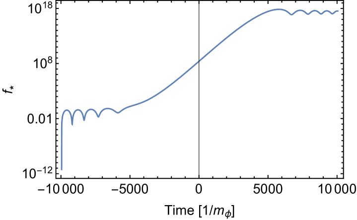
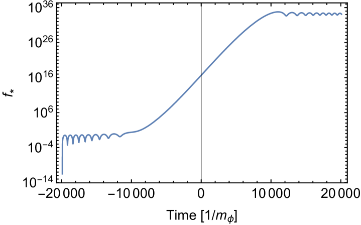
Figure 4: Evolution of $f_{\star}$, taking $q=10^{-2}$ and $H=10^{-2}q^{2}\ m_{\phi}$ (for which $t_{\pm}\simeq\mp 5000\ m_{\phi}^{-1}$).

Figure 5: Evolution of $f_{\star}$, taking $q=10^{-2}$ and $H=5\times 10^{-3}\ q^{2}m_{\phi}$ (for which $t_{\pm}\simeq\mp 10000\ m_{\phi}^{-1}$).

For the case that $f_{\star}(t_{-})\gg 1$, the total amount of the increase of $f_{\star}$ can be estimated by using the growth rate $\lambda_{k}$ given in the previous section. Because the enhancement of $f_{\star}$ occurs when the mode is in the resonance band, we concentrate on the epoch of $t_{+}\leq t\leq t_{-}$; during such an epoch, the occupation number is expected to evolve as $\dot{f}_{k}\simeq kH(\partial f_{k}/\partial k)+\lambda_{k}f_{k}$. Then, adopting the growth rate given in Eq. (3.30), $\dot{f}_{\star}$ is given by

$$\dot{f}_{\star}\simeq\sqrt{\frac{1}{4}q^{2}m_{\phi}^{2}-\left(2\Omega-m_{\phi}\right)^{2}}f_{\star},$$ (4.18)

which results in

$$\frac{f_{\star}(t_{-})}{f_{\star}(t_{+})}\simeq\exp\left[\int_{t_{+}}^{t_{-}}dt^{\prime}\sqrt{\frac{1}{4}q^{2}m_{\phi}^{2}-\left(2\Omega-m_{\phi}\right)^{2}}\right].$$ (4.19)

For the case that the mass of $\chi$ is negligible, the above ratio is estimated as [20, 22, 23]

$$\frac{f_{\star}(t_{-})}{f_{\star}(t_{+})}\simeq\exp\left(\frac{\pi q^{2}m_{\phi}}{8H}\right).$$ (4.20)

In order for a significant enhancement of the occupation number, $H$ should be smaller than $q^{2}m_{\phi}$.

To show the validity of the above estimation, we calculate the ratio $f_{\star}(t_{-})/f_{\star}(t_{+})$ by using Eq. (4.20) and also by numerically solving Eqs. (4.10) $-$ (4.12); for the numerical calculation, we adopt the setup given by Eqs. (4.13), (4.14), and (4.17). The results are shown in Table 2 for several values of $H$. We can find an excellent agreement between the numerical result and the semi-analytic result given in Eq. (4.20), even though an enormous increase of $f_{\star}$ occurs while the mode is in the resonance band.

$h$	Numerical	Eq. (4.20)	Eq. (4.23)
$2\times 10^{-2}$	$8.4\times 10^{8}$	$3.4\times 10^{8}$	$5.8\times 10^{16}$
$1\times 10^{-2}$	$1.7\times 10^{17}$	$1.1\times 10^{17}$	$6.4\times 10^{33}$
$5\times 10^{-3}$	$1.0\times 10^{34}$	$1.3\times 10^{34}$	$8.3\times 10^{67}$

Table 2: The ratio $f_{\star}(t_{-})/f_{\star}(t_{+})$, based on the numerical calculation (Numerical) and Eq. (4.20), taking $q=10^{-2}$. We take several values of $q$ and $H$ (parameterized as $H=hq^{2}m_{\phi}$). For comparison, we also show the value of the right-hand side of Eq. (4.23).

4.2 Breakdown of Boltzmann equation

Finally, let us come to our main point. We compare the above results with that obtained by using the Boltzmann equation. Adopting the collision term given in Eq. (3.32), the Boltzmann equation with the cosmic expansion is

$$\dot{f}_{k}=Hk\frac{\partial f_{k}}{\partial k}+2\Gamma_{\phi\to\chi\chi}^{(0)}n_{\phi}\delta(k-p_{\chi})(1+2f_{k})\left(\frac{p_{\chi}^{2}}{2\pi^{2}}\right)^{-1},$$ (4.21)

or equivalently,

$$\dot{f}_{\star}=2\Gamma_{\phi\to\chi\chi}^{(0)}n_{\phi}\delta(K-p_{\chi})(1+2f_{\star})\left(\frac{p_{\chi}^{2}}{2\pi^{2}}\right)^{-1}.$$ (4.22)

One can easily solve this equation and obtain

$$f_{\star}(t\rightarrow\infty)=\frac{1}{2}\left[\exp\left(\frac{\pi q^{2}m_{\phi}}{4H}\right)-1\right].$$ (4.23)

We can see that, when the effect of the stimulated emission is effective, the enhancement factor suggested from the Boltzmann equation is exponentially larger than that from the argument based on the QFT (see Eq. (4.20)); the exponent is doubled in the result from the Boltzmann equation. (For comparison, we also show the right-hand side of (4.23) in Table 2.) Notice that the discrepancy in the present case is rather serious than that in the flat spacetime. This is because, here, we consider the evolution of the mode with a fixed comoving momentum which goes through the resonance band; thus the discrepancy cannot be solved even if we consider a prescription to average the growth rate in the resonance band.

We may naïvely set an ansatz for a Boltzmann equation with including the quantum effect. We can find that the result based on the QFT is well described by Eq. (4.21) with replacing $(1+2f_{k})\rightarrow(1+f_{k})$ in the right-hand side, i.e.,

$$\dot{f}_{k}=Hk\frac{\partial f_{k}}{\partial k}+2\Gamma_{\phi\to\chi\chi}^{(0)}n_{\phi}\delta(k-p_{\chi})(1+f_{k})\left(\frac{p_{\chi}^{2}}{2\pi^{2}}\right)^{-1}.$$ (4.24)

The solution of the above equation is given by

$$f_{\star}(t\rightarrow\infty)=\exp\left(\frac{\pi q^{2}m_{\phi}}{8H}\right)-1,$$ (4.25)

which has the same growing behavior as that in the QFT (see Eq. (4.20)). Interestingly, Eq. (4.25) well describes the numerical result for any value of $f_{\star}(t\rightarrow\infty)$. The theoretical justification of this equation will be considered in the future [39].

5 Summary

In this paper, we have studied particle production from an oscillating scalar field $\phi$, assuming that the final state particle $\chi$ is very weakly interacting. We have paid particular attention to the consistency of the results from the Boltzmann equation and those from the QFT calculation. We have concentrated on the case that the production of $\chi$ is via the process $\phi\rightarrow\chi\chi$.

First, we have considered particle production in the flat spacetime. In such a case, we have discussed the evolution of the occupation number of each mode (i.e., mode with a fixed momentum $k$) separately in the narrow resonance regime. We have derived the evolution equations for the occupation number of each mode based on the QFT. A resonance band shows up at $\omega_{k}$ close to $\frac{1}{2}m_{\phi}$, which corresponds to the lowest resonance band in the context of the parametric resonance. The modes within the resonance band can be effectively produced. For the timescale much longer than $(qm_{\phi})^{-1}$, the occupation numbers of the modes in the resonance band exponentially grow; the growth rate obtained in our analysis is consistent with that given by the study of the parametric resonance using the Mathieu equation. Then, comparing the occupation number obtained from the QFT calculation with that from the Boltzmann equation, we have found that they do not agree well when the occupation number is larger than $\sim 1$. On the contrary, when $f_{k}\ll 1$, we have found a good agreement of two results. We have also argued how our evolution equation based on the QFT could be related to the ordinary Boltzmann equation. When the occupation number is larger than $\sim 1$, some of the approximation and assumption necessary for such an argument cannot be justified, which, we expect, causes the disagreement.

Then, we have studied particle production taking into account the effects of cosmic expansion. With the cosmic expansion, the physical momentum redshifts. The momentum of each mode stays in the resonance band for a finite amount of time and then exits the resonance band. The exponential growth of the occupation number occurs only in the resonance band. The growth factor has been studied numerically and analytically, adopting the evolution equations based on the QFT. The agreement between numerical and analytical results is excellent. We have also analyzed the system by using the conventional Boltzmann equation and found that the growth rate obtained by solving the Boltzmann equation is a factor of $2$ larger than that based on the QFT. Thus, the occupation number from the Boltzmann equation may become exponentially larger than that from the QFT, and a naïve use of the conventional Boltzmann equation may result in a significant overestimation of the number density of $\chi$.

In this paper, we have considered the production of a bosonic particle, concentrating on the lowest resonance band of the parametric resonance. Consideration of the production of fermionic particles and the study of the higher resonance bands, as well as the use of the evolution equations based on the QFT to other phenomena, are left as future works [39].

Appendix A QFT and Boltzmann Equation

In this Appendix, we give a discussion which may indicate a potential reason of the break down of the Boltzmann equation in the QFT.

We start with

$$\frac{1}{T}\int_{-T/2}^{T/2}{dte^{\pm im_{\phi}t}\dot{g}_{k}}=\mp\frac{1}{T}\int_{-T/2}^{T/2}{im_{\phi}e^{\pm im_{\phi}t}g_{k}dt}+\frac{1}{T}\left[e^{\pm im_{\phi}t}g_{k}\right]^{T/2}_{-T/2}.$$ (A.1)

Then, let us assume that $\lim_{T\to\infty}\frac{1}{T}g_{k}(\pm T/2)\rightarrow 0$, although it cannot be satisfied as we will see in the following. The assumption may imply that the state is asymptotically an eigenstate of the particle numbers, like in the perturbation theory of the QFT. Then the second term of the right hand side of Eq. (A.1) vanishes in the limit of $T\rightarrow\infty$.

Then, we use the following relation obtained from (3.15):

$$(2k\mp m_{\phi}-i\epsilon)\int_{-T/2}^{T/2}dte^{\pm im_{\phi}t}g_{k}=-\int_{-T/2}^{T/2}dt\left[\frac{A\phi(t)}{\omega_{k}}(1+2f_{{k}}+g_{k})e^{\pm im_{\phi}t}-i\epsilon e^{\pm im_{\phi}t}g_{k}\right],$$ (A.2)

or equivalently,

$$\frac{1}{T}\int_{-T/2}^{T/2}{e^{\pm im_{\phi}t}g_{k}dt}=-\frac{1}{T}\frac{1}{(2k\mp m_{\phi})-i\epsilon}\frac{A\bar{\phi}}{\omega_{k}}\int_{-T/2}^{T/2}dt(1+2f_{{k}})e^{\pm im_{\phi}t}\cos m_{\phi}t+O(\epsilon,q^{2}).$$ (A.3)

At the end of calculation, we take $\epsilon\rightarrow+0$. Using $\lim_{\epsilon\to+0}\Im(x-i\epsilon)^{-1}=\pi\delta(x)$, the time average of Eq. (3.14) becomes

$$\langle\dot{{f}}_{{k}}\rangle_{t}=\frac{\pi q^{2}m_{\phi}}{16}\frac{2p_{\chi}}{m_{\phi}}\left(1+2\langle{{f}_{k}\rangle}_{t}\right)\delta(k-m_{\phi}/2)+O(q^{3}).$$ (A.4)

Thus, if $\frac{1}{T}g_{k}(T/2)=0$ (with taking $\epsilon>0$), we obtain the collision term in the Boltzmann equation (3.32). However, $\frac{1}{T}g_{k}(T/2)=0$ does not hold in the limit of $T\rightarrow\infty$. To see this, we can use the following quantity:

$$J_{k}\equiv\left(f_{k}+\frac{1}{2}\right)^{2}-|g_{k}|^{2},$$ (A.5)

which is time independent, i.e.,

$$\dot{J}_{k}=0.$$ (A.6)

With the initial condition of our choice, $J_{k}=\frac{1}{4}$. For $k$ in the resonance band, $\frac{1}{T}g_{k}(T/2)$ diverges as $T\rightarrow\infty$ because of the exponential growth of $f_{k}$. As a result, we may conclude that the Boltzmann equation cannot be derived because the state at $t\rightarrow\infty$ is not an eigenstate of the particle numbers.

References

- [1] E. W. Kolb and M. S. Turner, “The Early Universe,” Front. Phys. 69, 1-547 (1990)
- [2] V. Mukhanov, “Physical Foundations of Cosmology,” Cambridge University Press (2005).
- [3] A. A. Starobinsky, Adv. Ser. Astrophys. Cosmol. 3, 130-133 (1987)
- [4] A. H. Guth, Adv. Ser. Astrophys. Cosmol. 3, 139-148 (1987)
- [5] K. Sato, Mon. Not. Roy. Astron. Soc. 195, 467-479 (1981) NORDITA-80-29.
- [6] A. D. Linde, Adv. Ser. Astrophys. Cosmol. 3, 149-153 (1987)
- [7] A. Albrecht and P. J. Steinhardt, Adv. Ser. Astrophys. Cosmol. 3, 158-161 (1987)
- [8] K. Enqvist and M. S. Sloth, Nucl. Phys. B 626, 395-409 (2002) [arXiv:hep-ph/0109214 [hep-ph]].
- [9] D. H. Lyth and D. Wands, Phys. Lett. B 524, 5-14 (2002) [arXiv:hep-ph/0110002 [hep-ph]].
- [10] T. Moroi and T. Takahashi, Phys. Lett. B 522, 215-221 (2001) [erratum: Phys. Lett. B 539, 303-303 (2002)] [arXiv:hep-ph/0110096 [hep-ph]].
- [11] J. Preskill, M. B. Wise and F. Wilczek, Phys. Lett. B 120, 127-132 (1983)
- [12] L. F. Abbott and P. Sikivie, Phys. Lett. B 120, 133-136 (1983)
- [13] M. Dine and W. Fischler, Phys. Lett. B 120, 137-141 (1983)
- [14] P. W. Graham and A. Scherlis, Phys. Rev. D 98, no.3, 035017 (2018) [arXiv:1805.07362 [hep-ph]].
- [15] F. Takahashi, W. Yin and A. H. Guth, Phys. Rev. D 98, no.1, 015042 (2018) [arXiv:1805.08763 [hep-ph]].
- [16] I. Affleck and M. Dine, Nucl. Phys. B 249, 361-380 (1985)
- [17] T. Moroi and W. Yin, [arXiv:2011.09475 [hep-ph]].
- [18] J. H. Traschen and R. H. Brandenberger, Phys. Rev. D 42, 2491-2504 (1990)
- [19] L. Kofman, A. D. Linde and A. A. Starobinsky, Phys. Rev. Lett. 73, 3195-3198 (1994) [arXiv:hep-th/9405187 [hep-th]].
- [20] Y. Shtanov, J. H. Traschen and R. H. Brandenberger, Phys. Rev. D 51, 5438-5455 (1995) [arXiv:hep-ph/9407247 [hep-ph]].
- [21] M. Yoshimura, Prog. Theor. Phys. 94, 873-898 (1995) [arXiv:hep-th/9506176 [hep-th]].
- [22] S. Kasuya and M. Kawasaki, Phys. Lett. B 388, 686-691 (1996) doi:10.1016/S0370-2693(96)01216-6 [arXiv:hep-ph/9603317 [hep-ph]].
- [23] L. Kofman, A. D. Linde and A. A. Starobinsky, Phys. Rev. D 56, 3258-3295 (1997) [arXiv:hep-ph/9704452 [hep-ph]].
- [24] J. F. Dufaux, G. N. Felder, L. Kofman, M. Peloso and D. Podolsky, JCAP 07, 006 (2006) [arXiv:hep-ph/0602144 [hep-ph]].
- [25] S. Matsumoto and T. Moroi, Phys. Rev. D 77, 045014 (2008) [arXiv:0709.4338 [hep-ph]].
- [26] T. Asaka and H. Nagao, Prog. Theor. Phys. 124, 293-314 (2010) [arXiv:1004.2125 [hep-ph]].
- [27] K. Mukaida, K. Nakayama and M. Takimoto, JHEP 12, 053 (2013) [arXiv:1308.4394 [hep-ph]].
- [28] N. Kitajima, T. Sekiguchi and F. Takahashi, Phys. Lett. B 781, 684-687 (2018) [arXiv:1711.06590 [hep-ph]].
- [29] M. A. Amin, J. Fan, K. D. Lozanov and M. Reece, Phys. Rev. D 99, no.3, 035008 (2019) [arXiv:1802.00444 [hep-ph]].
- [30] M. A. G. Garcia and M. A. Amin, Phys. Rev. D 98, no.10, 103504 (2018) doi:10.1103/PhysRevD.98.103504 [arXiv:1806.01865 [hep-ph]].
- [31] P. Agrawal, N. Kitajima, M. Reece, T. Sekiguchi and F. Takahashi, Phys. Lett. B 801, 135136 (2020) [arXiv:1810.07188 [hep-ph]].
- [32] J. A. Dror, K. Harigaya and V. Narayan, Phys. Rev. D 99, no.3, 035036 (2019) [arXiv:1810.07195 [hep-ph]].
- [33] R. T. Co, A. Pierce, Z. Zhang and Y. Zhao, Phys. Rev. D 99, no.7, 075002 (2019) [arXiv:1810.07196 [hep-ph]].
- [34] K. Kaneta, Y. Mambrini and K. A. Olive, Phys. Rev. D 99, no.6, 063508 (2019) [arXiv:1901.04449 [hep-ph]].
- [35] K. D. Lozanov, [arXiv:1907.04402 [astro-ph.CO]].
- [36] G. Alonso-Álvarez, R. S. Gupta, J. Jaeckel and M. Spannowsky, JCAP 03, 052 (2020) [arXiv:1911.07885 [hep-ph]].
- [37] E. Mathieu, “Mémoire sur Le Mouvement Vibratoire d’une Membrane de forme Elliptique,” Journal de Mathématiques Pures et Appliquées, 137-203 (1868).
- [38] M. William. “Theory and application of Mathieu functions,” Oxford University Press (1951).
- [39] T. Moroi and W. Yin, work in progress.