Learning Effective Spin Hamiltonian of Quantum Magnet

Abstract

Interacting spins in quantum magnet can cooperate and exhibit exotic states like the quantum spin liquid. To explore the materialization of such intriguing states, the determination of effective spin Hamiltonian of the quantum magnet is thus an important, while at the same time, very challenging inverse many-body problem. To efficiently learn the microscopic spin Hamiltonian from the macroscopic experimental measurements, here we propose an unbiased Hamiltonian searching approach that combines various optimization strategies, including the automatic differentiation and Bayesian optimization, etc, with the exact diagonalization and many-body thermal tensor network calculations. We showcase the accuracy and powerfulness by applying it to training thermal data generated from a given spin Hamiltonian, and then to realistic experimental data measured in the spin-chain compound Copper Nitrate and triangular-lattice materials TmMgGaO₄. This automatic Hamiltonian searching constitutes a very promising approach in the studies of the intriguing spin liquid candidate magnets and correlated electron materials in general.

Introduction.— Exotic many-body quantum states and phenomena in magnetic materials have raised great research interest recently. Among others, an intriguing topic is the materialization of quantum spin liquids with topologically ordered ground states and anyonic excitations, which has been long pursued in quantum magnetism  Anderson (1973); Kitaev (2006); Zhou et al. (2017); Balents (2010). Some prominent spin liquid candidate systems include the kagome Han et al. (2012); Fu et al. (2015), triangular Shimizu et al. (2003); Yamashita et al. (2010); Liu et al. (2018), and Kitaev magnets Jackeli and Khaliullin (2009); Chaloupka et al. (2010); Ye et al. (2012); Banerjee et al. (2017). However, the lack of precise knowledge on the effective spin lattice models of these frustrated magnets hinders the unambiguous understanding of the quantum states and phases therein.

The identification of the microscopic spin model and the determination of Hamiltonian parameters of the magnetic materials constitute an important step towards understanding their properties. It is, however, a very challenging problem to “learn” the spin Hamiltonian from experimental measurements. For example, to understand the quantum states in the prominent Kitaev materials $\alpha$-RuCl₃, various spin models have been proposed, yet none of them could satisfactorily explain all experimental observation Laurell and Okamoto (2020). The difficulty is two-fold. Firstly, to solve the spin Hamiltonian and compute the thermodynamic and dynamic properties that are experimentally relevant is by no means an easy problem, as there is a many-body exponential wall to break. Secondly, even worse, the determination of the effective spin Hamiltonian from experimental measurements constitutes an inverse many-body problem.

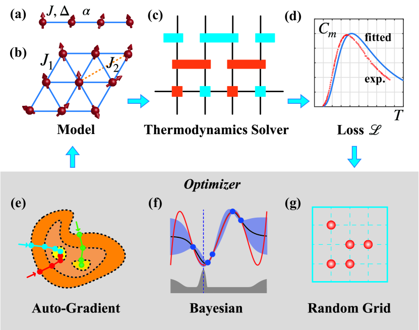
Figure 1: The workflow of automatic Hamiltonian searching. (a,b) show the HAFC model with coupling $J$, ratio $\alpha$ and magnetic anisotropy $\Delta$, and frustrated triangular-lattice model with nearest-neighboring coupling $J_{1}$ and next-nearest-neighboring coupling $J_{2}$. With the thermodynamics solvers in (c), we can compute the (d) loss function $\mathcal{L}$, and feed it to the optimizers including (e) auto-gradient, (f) Bayesian, and (g) random grid methods. The optimizer proposes a new trial parameter set for the next iteration, until the convergence criteria is reached.

The recent progress in finite-temperature tensor networks has been swift, which enables efficient and accurate calculations of the thermodynamic properties of large-scale 1D and 2D systems down to low temperature Bursill et al. (1996); Wang and Xiang (1997); Xiang (1998); Feiguin and White (2005); White (2009); Stoudenmire and White (2010); Li et al. (2011); Dong et al. (2017); Chen et al. (2017, 2018); Li et al. (2019). Nevertheless, these thermal tensor network calculations generically demands considerable computational resources for low-temperature simulations. Therefore, considering a realistic magnetic material [c.f. Eqs. (2, Learning Effective Spin Hamiltonian of Quantum Magnet, 4) below], grid searching by computing the many-body systems point by point in the parameter space and compare to to experimental data, is a very laborious and, even unfeasible for Hamiltonians with, say, more than 5 parameters in practice.

Machine learning techniques have recently brought into quantum many-body computations very helpful new perspectives and methodology. For example, it has been proposed that the artificial neural networks can serve as a powerful variational many-body wavefunction ansatz that produces accurate results Carleo and Troyer (2017), and the differentiable tensor network approach helps to design novel tensor renormalization group algorithms with improvement Liao et al. (2019); Chen et al. (2020). On the other hand, the many-body tensor network approaches have also found their applications in machine learning, including the matrix product state and tree tensor network based supervised learning Stoudenmire and Schwab (2016); Liu et al. (2019), the Bayesian tensor-network probabilistic learning  Ran (2020), and many others Cichocki et al. (2017); Han et al. (2018); Glasser et al. (2019).

In this work, we propose an automatic Hamiltonian searching approach for determining the effective spin model — the magnetism genome — from fitting thermodynamic data of quantum magnetic materials. Our method explores the parameter space efficiently, with gradient optimization by automatic differentiation (auto-gradient) and Bayesian optimization schemes, inspired by machine learning techniques. In particular, the predicted landscape of loss function in the parameter space can present a comprehensive information, and is thus of great helpfulness in, e.g., reducing the human bias in the parameter fittings. The automatic Hamiltonian searching, given it auto-gradient or Bayesian, are very flexible and can be combined with various many-body methods, ranging from small-size exact diagonalization (ED, as a high-$T$ solver) to large-scale (even infinite-size) thermal tensor networks (low-$T$ solver) Li et al. (2011); Dong et al. (2017); Chen et al. (2018); Li et al. (2019), and other thermodynamics solvers SM .

Thermodynamics many-body solver.— When only high-$T$ thermal data are involved, the ED calculations can be employed to compute the spin lattice model with limited system sizes. The effective thermal correlation length is short, and it thus serves only as a high-$T$ solver. Nevertheless, we find ED calculations are already very helpful for automatic determination of the spin Hamiltonians, as the valuable correlations and thus interactions information “hidden” in the quantitative details of the thermodynamic curves (though featureless to human eyes) can be efficiently extracted by optimization techniques widely used in machine learning.

Moreover, to unambiguously determine the spin Hamiltonian, we employ large-scale tensor network methods as the low-$T$ thermodynamic solver. Linearized tensor renormalization group (LTRG) Li et al. (2011); Dong et al. (2017) can compute infinite-length system and thus provide an accurate access to the full-temperature range of spin-chain materials. Beyond 1D system, other thermal tensor network methods including the exponential tensor renormalization group Chen et al. (2018); Li et al. (2019), and tensor product state approaches Li et al. (2011); Czarnik and Dziarmaga (2014) can be used to compute large-scale 2D systems, which can also be conveniently combined with either auto-gradient or Bayesian optimization schemes will be discussed below shortly.

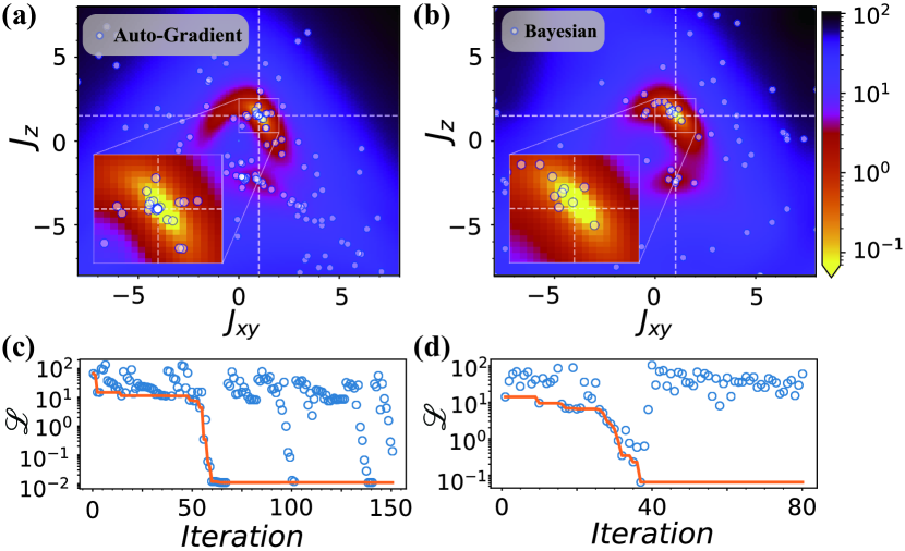
Figure 2: (a) The scatters indicate the evaluated queries of 150 iterations of multi-restart gradient optimization processes, and the background, $\mathcal{L}$ landscape, is obtained via a grid search. (b) Landscape of $\mathcal{L}$ predicted by the Bayesian optimization with an evaluated query of 80 parameter points, where the loss along indicated dash lines can be found in Supplementary Fig. S4 (b,c). (c, d) Solid lines indicate the convergence of $\mathcal{L}$ using respectively multi-restart auto-gradient and Bayesian optimizations, and the scatters represent the evaluated function value $\mathcal{L}(\mathbf{x}_{i})$ at each iteration.

Random grid, auto-gradient and Bayesian optimization.— The objective loss function of the thermal data fitting reads

$$\mathcal{L}(\mathbf{x}_{i})=\sum_{\alpha}\frac{1}{N_{\alpha}}\lambda_{\alpha}(\frac{O^{\rm exp}_{\alpha}-O^{\rm sim}_{\alpha}}{O^{\rm sim}_{\alpha}})^{2},$$ (1)

where $O^{\rm exp}_{\alpha}$ and $O^{\rm sim}_{\alpha}$ (with $\alpha$ labeling different physical quantities) are the experimental and simulated quantities, respectively, and $\lambda_{\alpha}$ is an empirical weight coefficient set to unity by default. The parameter vector $\mathbf{x}$ contains various components including $J$, $\Delta$ and $g$, and span a parameter space $\mathcal{X}$. $N_{\alpha}$ is the data point number of quantity $O_{\alpha}$, and thus $1/N_{\alpha}$ normalizes the loss function per point .

An efficient optimizer that minimizes the loss function $\mathcal{L}$ in the parameter space $\mathcal{X}$ plays an indispensable role in the automatic Hamiltonian searching. In this work, we have employed two machine-learning inspired algorithms: auto-gradient and Bayesian searching, and compare them to a plain random grid method SM .

In particular, inspired by the backpropagation arithmetic in deep learning LeCun et al. (2015), automatic differentiation has been introduced into tensor-network methods for quantum many-body computations Liao et al. (2019); Chen et al. (2020). Here in our work, to obtain the gradient information that greatly facilitates the search of spin Hamiltonians, we realize the differentiable programming of the thermodynamics solver. The basic idea is that, given the many-body solver fully differentiable, the derivatives between intermediate variables of adjacent steps are stored in the forward process all the way to the final loss function $\mathcal{L}$. Given that, the derivatives of the loss function respective to the Hamiltonian parameters, ${\bf{\bar{x}}_{i}}=\partial\mathcal{L}/\partial{\bf{x}_{i}}$, can be computed automatically following the derivative chain rule in the backward propagations, which can be further utilized to optimize the parameters $\bf{x}_{i}$ via gradient-based optimizer SM . As the loss $\mathcal{L}$ is generically non-convex (c.f. Fig. 2), we need to restart and perform the auto-gradient search for multiple times, in order to guarantee the convergence to global minimum.

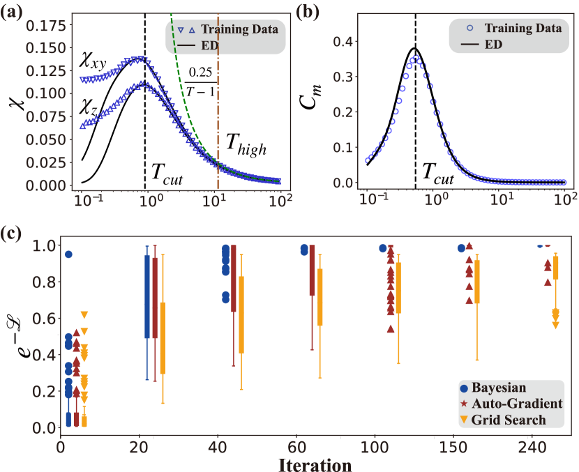
Figure 3: (a) The in-plane $\chi_{xy}^{\,}$ and out-of-plane $\chi_{z}^{\,}$ of the training data generated by an infinitely-long XXZ chain with $J_{z}=1.5,J_{xy}=1$ (hollow symbols) and a best fitting based on 10-site ED calculations with parameters $J_{z}=1.49(1),J_{xy}=1.02(1)$ (solid line). Only “experimental" data with temperatures higher than $T_{\rm cut}$ (black dashed line) are involved in the fittings. Below the temperature scale $T_{high}$ (brown dash-dotted line), the susceptibility $\chi$ deviates from the Curie-Weiss behaviors marked with the green dashed line. (b) The magnetic specific heat $C_{m}$ of training experiment and optimal ED fitting. (c) The box plot of best $\mathcal{L}$ found at $n$-th iteration of 100 independent experiments with three optimization schemes.

The Bayesian optimization (BO) is a powerful and highly efficient method which has been widely used in hyper-parameter tuning of deep neural networks, active, and reinforce learning, etc Shahriari et al. (2016). As most of the state-of-the-art thermodynamics many-body solvers are computationally costly, it is then essential to exploit the information of tested parameter points and determine where to evaluate the function next Melnikov et al. (2018).

In practice, BO minimizes our loss function $\mathcal{L}$ by iteratively updating a statistical model $\mathcal{GP}:\mathcal{X}\rightarrow\mu,\sigma$ over the entire parameter space $\mathcal{X}$, and $\mu,\sigma$ represent the predicted value and uncertainty, as shown in Fig. 1(f). The parameters $\bf{x}$ to be evaluated at each iteration is determined by maximizing an acquisition function $\alpha_{\rm EI}(\mathbf{x})$, based on the expected improvement. To be specific, one can determine $\mathbf{x}_{n+1}=\arg\max\alpha_{\rm EI}(\mathbf{x})=\arg\max\mathbb{E}[\mathcal{L}_{n,min}-\mu_{n}(\mathbf{x})]$ as the best parameter candidate in the next ($n+1$) iteration, where $\mathcal{L}_{n,min}$ denotes the minimal loss function found in the $n$-th iteration. This method can elegantly balance the optimization efficiency and the exploration of parameter space $\mathcal{X}$ by choosing the appropriate acquisition criteria SM .

Refind the spin Hamiltonian.— We start with training thermal data generated from the XXZ Heisenberg antiferromagnetic chain (HAFC) model with a given parameter, and feed the “experimental” data to various optimizers, i.e., random grid, auto-gradient, and the Bayesian searching, to see if we can refind the correct Hamiltonian parameters. Below, we stick to an thermodynamics ED solver, and focus on the comparison between various optimization schemes.

The thermodynamic data of HAFC systems are computed from the model Hamiltonian below, i.e.,

$$H=\sum_{\langle i,j\rangle}J_{xy}(S_{i}^{x}S_{j}^{x}+S_{i}^{y}S_{j}^{y})+J_{z}S_{i}^{z}S_{j}^{z},$$ (2)

where $\langle i,j\rangle$ represents a nearest-neighboring pair of sites. We employ LTRG to generate the infinite-chain thermal data of HAFC with $J_{xy}=1$ and $J_{z}=1.5$ (for cases with different $J_{z}$ values, see Supplementary Fig. S4). Gaussian noises $\mathcal{N}(0,0.01\times E_{i})$ are added to each data point of mean value $E_{i}$ are also introduced (c.f. Fig. 3), to mimic the measurement errors in real experiments. We show below that the smart optimizers and the high-$T$ ED solver can cooperate and do a surprisingly good job to “learn” the correct Hamiltonian parameters.

As shown in Fig. 2(a), the loss function landscape scanned throughout the whole parameter space $\mathcal{X}$ is found to have a global minimal at around $J_{xy}=1$ and $J_{z}=1.5$, exactly the input model parameter set, which delivers a key information that one can, in principle, locate the correct interaction parameters even from high-$T$ thermodynamics. Indeed, both the auto-gradient and BO schemes can efficiently and accurately find the original parameters. The latter can also reproduce the correct loss landscape, c.f. Fig. 2(a,b). In the automatic Hamiltonian searching, as the ED thermodynamics solver can only simulate relatively high-$T$ properties, so we introduce a cut-off temperature $T_{\rm cut}$ in the fitting. As shown in Fig. 3(a,b), we only fit thermal data at $T\gtrsim T_{\rm cut}\simeq O(1)$, which are chosen as the peak positions of magnetic susceptibility and specific heat curves, respectively. The dependence of determined Hamiltonian parameters on $T_{\rm cut}$ is discussed in the SupplementarySM .

Notably, in the definition of $\mathcal{L}$, c.f. Eq. (1), when only $C_{m}$ and $\chi_{z}$ are included, the optimizers can find two optimal parameters $J_{xy}=\pm 1$ and $J_{z}=1.5$, which is very interesting as indeed the two parameter points have exactly the same thermodynamic traits, as the Hamiltonian Eq. (2) has the same energy spectra for $J_{xy}=\pm 1$, and the our smart approach can automatically find this fact out. Nevertheless, higher resolution can be achieved by adding more thermal data to the fittings. The two-fold degeneracy in landscape can be removed once $\chi_{xy}$ is introduced to $\mathcal{L}$. As a result, in Fig. 2(a,b) and Fig. 3 we have included the specific heat $C_{m}$, both in-plane and out-of-plane magnetic susceptibilities $\chi_{xy}$ and $\chi_{z}$, and the model parameters is now uniquely pinpointed SM .

From Fig. 3(c), in the 100 independent searching experiments, we note that both the Bayesian and auto-gradient approaches clearly outperforms the random grid method in both efficiency and accuracy [c.f. also Fig. 2(c,d)]. Although the auto-gradient method can lead to very accurate estimate in the “lucky" case (c.f. Fig. 2), it also has good chance to be trapped in the local minimal, especially when the optimization iteration number is relatively small. On the other hand, the Bayesian optimization is mostly stable amongst three schemes, and it finds the optimal parameters $J_{xy}=1.025(9)$ and $J_{z}=1.49(1)$ very efficiently. Due to this reason, and also that the Bayesian optimization is more flexible and can be combined with various many-body solvers, below we mainly adopt the Bayesian approach and apply it to study realistic magnetic materials.

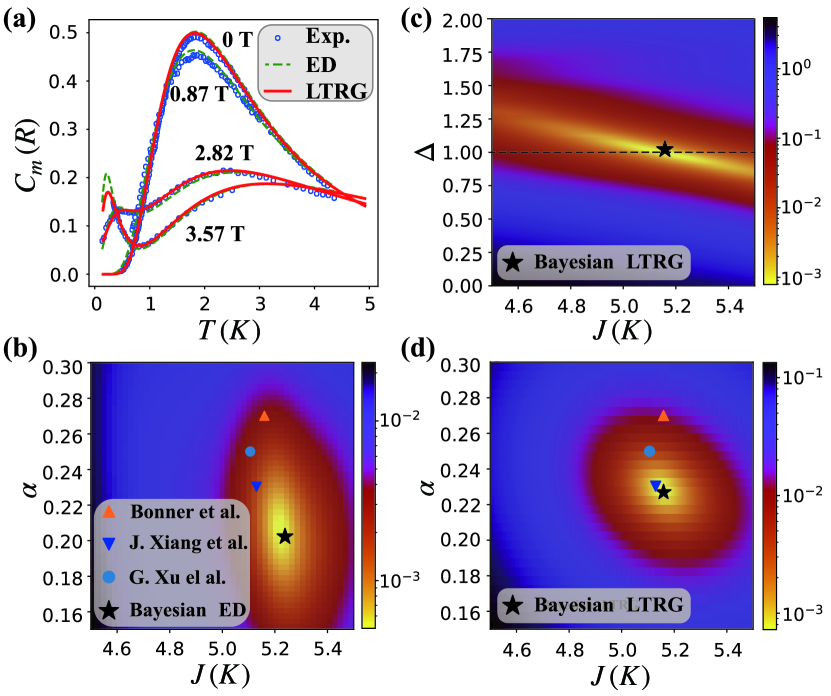
Figure 4: (a) Magnetic specific heat $C_{m}/R$ at various fields of 0, 0.87, 2.82, and 3.57 T. The dashed lines represent the ED fittings and the solid lines are LTRG calculations. (b) shows the Bayesian $\mathcal{L}$ landscape within the $J-\alpha$ plane, using ED solver, where the estimated optimal parameter point (the asterisk) are compared to results in previous studies van Tol et al. (1971); Xu et al. (2000); Xiang et al. (2017). (c, d) The Bayesian $J-\alpha$ (with fixed $\Delta=1$, $g=2.31$) and $J-\Delta$ ($\alpha=0.23$, $g=2.31$ fixed) landscape, obtained after 400 iterations of LTRG calculations. The optimal parameter found is $J=5.16(2)$ K, $\alpha=0.227(3)$, $\Delta=1.01(1)$, $g=2.237(8)$, which are very close to the estimated parameters in Ref. Xiang et al. (2017), and has a slightly smaller loss $\mathcal{L}=7.4\times 10^{-4}$.

Quantum spin-chain material Copper Nitrate.— Given the successful benchmark calculations on the training data set, we now move on to a realistic spin-chain material Copper Nitrate, Cu(NO₃)${}_{2}\,\cdot\,$2.5H₂O, whose magnetic interactions are described by the alternating Heisenberg XXZ model [c.f. Fig. 1(a)]  Berger et al. (1963); van Tol et al. (1971); Xu et al. (2000); Xiang et al. (2017), i.e.,

$$H = J\sum_{n=1}^{L/2}[(S_{2n-1}^{x}S_{2n}^{x}+S_{2n-1}^{y}S_{2n}^{y}+\Delta S_{2n-1}^{z}S_{2n}^{z})$$

$$+ \alpha\,(S_{2n}^{x}S_{2n+1}^{x}+S_{2n}^{y}S_{2n+1}^{y}+\Delta S_{2n}^{z}S_{2n+1}^{z})]$$

$$- g\mu_{B}B\sum_{i=1}^{L}S_{i}^{z}.$$

Therefore, the problem is to search for the minimal loss $\mathcal{L}$ within a four-dimensional parameter space, spanned by the parameter vectors $\bf{x}_{i}$ containing the coupling $J$, ratio $\alpha$, magnetic anisotropy $\Delta$, and the Landé factor $g$.

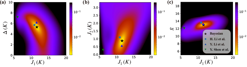
Figure 5: Loss landscape in (a) $J_{1}$-$\Delta$, (b) $J_{1}$-$J_{2}$, and (c) $J_{1}$-$g$ planes, obtained after 300 iterations of Bayesian optimization. The estimated Hamiltonian parameters with $J_{1}=11.5(1)$ K, $J_{2}=0.89(7)$ K, $\Delta=5.32(6)$ K, and $g=13.00(3)$, are labeled by the asterisk and compared to the solid circle, upper, and lower triangles that represent the previously fitted parameters from Refs. Li et al. (2020a, b); Shen et al. (2019).

In Fig. 4, we have employed ED and LTRG as our high- and low-$T$ thermodynamics solver, and find the model parameters automatically by fitting the specific heat and magnetic susceptibility measurements, above the intermediate temperature $T_{\rm cut}$. With the ED solver, we find the so-obtained $J-\alpha$ landscape [c.f. Fig. 4(c)] has a relatively narrow distribution in $J$ while a large uncertainty in alternating ratio $\alpha$. However, by using the LTRG thermodynamics solver of infinite chains, we get a significantly improved resolution, and find the optimal parameters very close to the previously determined model parameters by manual fittings Xiang et al. (2017).

In plotting the landscape in Fig. 4(b,d), we fix $\Delta=1$ [or very close to 1 in Fig. 4(d)], as it has been generally believed that the CN constitutes an isotropic Heisenberg spin chain van Tol et al. (1971); Xu et al. (2000) (although it has not been carefully examined before). With the automatic parameter searching, we show in Fig. 4(c) that $\Delta$ lies within a very narrow regime around 1, and no essential XXZ anisotropy is there in Copper Nitrate.

Triangular-lattice quantum Ising magnet TmMgGaO₄.— Now we switch to a 2D frustrated quantum magnet, and take the triangular-lattice rare-earth magnet TmMgGaO₄ as an example Cevallos et al. (2018); Shen et al. (2019); Li et al. (2020b, a). The precise determination of the spin Hamiltonian plays an indispensable role for understanding the emergent U(1) symmetry and topological Berezinskii-Kosterlitz-Thouless phase transitions in this quantum magnet Li et al. (2020b); Hu et al. (2020). In previous studies, the effective low-energy spin Hamiltonian of TmMgGaO₄ is found to fall into a triangular-lattice Ising model [c.f. Fig. 1(b)], i.e.,

$$H=J_{1}\sum_{\langle i,j\rangle}S_{i}^{z}S_{j}^{z}+J_{2}\sum_{\langle\langle i,j^{\prime}\rangle\rangle}S_{i}^{z}S_{j^{\prime}}^{z}-\Delta\sum_{i}S_{i}^{x}-g\mu_{B}B\sum_{i}S_{i}^{z},$$ (4)

where $J_{1}$ and $J_{2}$ are nearest-neighboring and next-nearest-neighboring Ising couplings, respectively, $\Delta$ is the intrinsic transverse field in the material (due to fine crystal-field splitting), and $g$ is the Landé factor.

We explore the $\mathcal{L}$-landscape in Fig. 5, employing a high-$T$ thermodynamics ED solver on a very small 9-site system (c.f. Supplementary SM for more details). Clearly, we see an optimal parameter point (asterisk) in Fig. 5, which is in very good consistent with two of previous model parameter estimates Li et al. (2020b, a), but different from that obtained from spin-wave fittings Shen et al. (2019).

Discussion and Outlook.— The determination of effective spin Hamiltonian paves the way towards understanding the exotic quantum states and phenomena, as well as designing future quantum applications, of the quantum magnetic materials. Solving the quantum many-body problem, i.e., computing the ground-state, thermodynamics, and dynamical properties from a spin lattice model constitutes a challenging problem. Therefore, at a first glance, the inverse problem — learning the microscopic model from macroscopic measurements — seems a problem intractable. Here, we show, through solving the artificial and realistic problems, that the inverse many-body problem can be elegantly resolved by combining the thermodynamics many-body solvers and Bayesian optimization.

The secrete lies in the fact that we actually do not need to solve a full many-body problem, but a much only a finite-temperature one that is numerically much easier to compute. Therefore, we find the ED solver that only accesses rather high-$T$ regime can already find the valuable interaction information, when combined with Bayesian optimization. Furthermore, with the powerful thermal tensor network method as a low-$T$ solver, a significantly improved resolution in Hamiltonian parameters can be obtained.

Our approach, in particular when combining the thermal tensor network approach and Bayesian optimization, can provide a very promising tool in studying quantum magnets and uncovering novel quantum states and phases therein. For example, the family of rare-earth Chalcogenides AReCh₂ (A for alkali or monovalent ions, Re is rare earth, and Ch is O, S, or Se) Liu et al. (2018); Zhang et al. (2020) shares a similar class of Hamiltonians with different coupling parameters. As there are abundant experimental thermodynamics data available, the approach established here allows us to search for the most promising quantum spin liquid candidates. Moreover, it also gives us the hope to build up a quantum magnetism genome library, by automatically finding the effective spin Hamiltonians for quantum magnetic materials, which are important for their future applications as, e.g., quantum critical coolant Zhitomirsky (2003); Zhitomirsky and Honecker (2004); Garst and Rosch (2005); Wolf et al. (2011); Gegenwart (2016) and spin-chain quantum information data bus Karbach and Stolze (2005); Cappellaro et al. (2007), etc. With the automatic Hamiltonian searching framework offered, and proof-of-principle examples tested, all these exciting exploration of correlated quantum materials can be started from here.

Acknowledgments.— W.L. thanks Shi-Ju Ran for the introduction to active learning and Bayesian optimization, and Lei Wang for stimulating discussions on the automatic differentiation. This work was supported by the NSFC through Grant Nos. 11974036 and 11834014. Source code relevant to this work and an interactive demo are available at this https URL.

Supplementary Materials:
Learning Effective Spin Hamiltonian of Quantum Magnet
Yu et al.

A Automatic Hamiltonian Searching Algorithms

Below we list three algorithms adopted in our Hamiltonian searching, which include the random grid (Algorithm 1), auto-gradient (Algorithm 2), and the Bayesian (Algorithm 3) methods. These three searching schemes can be combined with various many-body thermodynamics solvers in a very flexible manner, rendering different resolutions in determining the Hamiltonian parameters.

1 Discretize the parameter space into a uniform grid with n nodes ($\mathbf{x}_{1},...,\mathbf{x}_{n}$);

2 for $i=1$ to $n$ do

3       Random select one of the unevaluated nodes $\mathbf{x}_{i}$ and calculate the $\mathcal{L}(\mathbf{x}_{i})$;

4       Mark $\mathbf{x}_{i}$ as evaluated.

Algorithm 1 Random Grid Searching

1 for $i=1$ to $n$ do

2       Random choose a starting point $\mathbf{x_{i}}$;

3       for $j=1$ to $n$ do

4             $x_{i,j+1}=x_{i,j}+\lambda B^{-1}\nabla f(x_{i,j})$, where $B$ is an approximate Hessian;

5             if EOF then

6                   go to 2

7            

8      

Algorithm 2 Multi-Restart Auto-Gradient

1 Initialize a statistical model;

2 for $i=1$ to $n$ do

3       select the next point $\mathbf{x}_{i+1}$ to evaluate by maximizing the acquisition function $\mathbf{x}_{i+1}=\mathop{\arg\max}_{\mathbf{x}}\alpha(\mathbf{x};\mathcal{D}_{i})$;

4       evaluate objective function $y_{i+1}$ at $\mathbf{x}_{i+1}$;

5       Augment data $\mathcal{D}_{i+1}=\{\mathcal{D}_{i},(\mathbf{x}_{i+1}),y_{i+1}\}$;

6       update statistical model with $\mathcal{D}_{i+1}$

Algorithm 3 Bayesian Optimization

B Automatic Differentiation

In this section, we provide more details of automatic differentiation used in our auto-gradient scheme. Automatic differentiation is a well-developed technique in neural networks and deep learning LeCun et al. (2015). A central ingredient of automatic differentiation is the so-called computational graph (see Fig. S1 for a typical computational graph for many-body calculations). To generate such a computational graph, one starts with the input parameters, goes through a number of intermediate computation nodes, and ends up with the final loss function.

To be specific, for the quantum many-body problems afore-mentioned in main text, starting with several Hamiltonian parameters, e.g., ${\bf x}\equiv\{J,\Delta,g,\cdots\}$, one defines the many-body model Hamiltonian $H({\bf x})$. Given it either ED or thermal tensor network calculations, the partition function $Z$ and thereafter thermodynamic observables $\{O_{\alpha}\}$, can be obtained. Basing on the calculated observables $\{O_{\alpha}\}$, a loss function can be properly designed [cf. Eq. (1)]. The above procedure constitutes a forward evaluation of the loss function, and henceforth a computational graph ${\bf x}\to H\to Z\to O_{\alpha}\to\mathcal{L}$ is generated (cf. the right-directed lines in Fig. S1).

On the fly of the forward process, the derivatives between adjacent computation nodes, i.e. $\{\frac{\partial H}{\partial\bf x},\frac{\partial Z}{\partial H},\frac{\partial O_{\alpha}}{\partial Z},\frac{\partial\mathcal{L}}{\partial O_{\alpha}}\}$, are stored. Thus the derivatives of loss function with respect to the input parameters can be evaluated automatically via a chain rule,

$$\frac{\partial\mathcal{L}}{\partial\bf x}=\frac{\partial\mathcal{L}}{\partial O_{\alpha}}\,\frac{\partial O_{\alpha}}{\partial Z}\,\frac{\partial Z}{\partial H}\,\frac{\partial H}{\partial\bf x}.$$ (S1)

In our cases, since the number of input parameters [components in $\bf{x}$, typically a few to $O(10)$] is larger than the output (just a single value of loss $\mathcal{L}$), it is therefore more efficient to evaluate Eq. (S1) following the reverse-mode automatic differentiation (i.e., from left to right on the right-hand side of the equation). In this work, we have implemented a differentiable ED calculation with Pytorch Paszke et al. (2019), and the generalization to tensor networks is also feasible Liao et al. (2019); Chen et al. (2020).

Figure S1: A typical computational graph of the quantum many-body calculations, with the forward process indicated by all the right-directed lines, and the backward process by the left-directed lines.

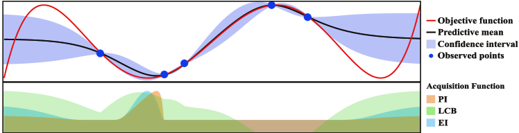
Figure S2: Red line in the upper panel represent the unknown objective function, with blue dots the evaluated points. The black line and shade represent the predicted mean and confidence interval, respectively. Various shades in the lower panel corespondent to different acquisition functions.

C Bayesian Optimization with Gaussian Process: Kernel Function, ARD and Acquisition Function

As shown in Algorithm 3 and Fig. S2, in the Bayesian optimization we need to iteratively update a statistical model that can be used to estimate the overall landscape of $\mathcal{L}$, based on history queries. In this work, we choose a commonly used statistical model called Gaussian process, which fits well our problem and is denoted as

$$\mathcal{GP}:\mathcal{X},\mathcal{D}\longrightarrow\mu,\sigma$$ (S2)

where $\mathcal{X}$ is the parameter space spanned by the parameter vectors $\bf{x}$, which could include, in practice, components $J,g,\Delta$, etc. The set of total $n$ history queries is noted as $\mathcal{D}_{n}=(({\bf{x}}_{1},y_{1}),({\bf{x}}_{2},y_{2}),...,({\bf{x}}_{n},y_{n}))$, with $y_{i}$ being the evaluated function value at parameter $\bf{x}_{i}$, i.e., $\mathcal{L}(\bf{x}_{i})$. Then by assuming a joint multivariate Gaussian distribution over $(y_{1},y_{2},...,y_{n};y_{n+1})$, with the covariances characterized by a kernel function $k(\bf{x}_{i},\bf{x}_{j})$, and $y_{n+1}$ to be estimated at ${\bf{x}}_{n+1}$, we can compute a posterior distribution of $y_{n+1}\sim\mathcal{N}(\mu_{n},\sigma_{n}^{2})$ by

$$\mu_{n}(\mathbf{x}_{n+1}) =\mathbf{k}(\mathbf{x}_{n+1})^{\mkern-1.5mu\mathsf{T}}\mathbf{K}^{-1}\mathbf{y},$$ (S3)

$$\sigma_{n}^{2}(\mathbf{x}_{n+1}) =\mathit{k}(\mathbf{x}_{n+1},\mathbf{x}_{n+1})-\mathbf{k}(\mathbf{x}_{n+1})^{\mkern-1.5mu\mathsf{T}}\mathbf{K}^{-1}\mathbf{k}(\mathbf{x}_{n+1}),$$ (S4)

where a constant zero prior mean is assumed in the space $\mathcal{X}$. ${\bf{y}}=(y_{1},y_{2},...,y_{n})^{\mkern-1.5mu\mathsf{T}}$ is the vector of evaluated function values, $\mathbf{k}(\mathbf{x})^{\mkern-1.5mu\mathsf{T}}=\left(k(\mathbf{x},\mathbf{x_{1}}),k(\mathbf{x},\mathbf{x_{2}}),...\right)$ and $\mathbf{K}_{i,j}=k(\mathbf{x}_{i},\mathbf{x}_{j})$ are respectively the covariance vector and matrix , where $\mathbf{x_{1}},\mathbf{x_{2}},...,\mathbf{x_{n}}$ represent the calculated parameter points in the history queries. The quality of GP regression to fit the real landscape is determined by the choice of kernel function $k(\bf{x},\bf{x}^{\prime})$. In practice, we chose a Matérn$-5$ kernel, i.e.,

$$\mathllap{\mathit{k}_{Mat\acute{e}rn5}(\bf{x},\bf{x}^{\prime})} =\theta_{0}^{2}\exp(-\sqrt{5})(1+\sqrt{5}r+\frac{5}{3}r^{2}),$$ (S5)

where in the kernel function $r^{2}=(\mathbf{x}-\mathbf{x}^{\prime})^{\mkern-1.5mu\mathsf{T}}\mathbf{\Lambda}(\mathbf{x}-\mathbf{x}^{\prime})$ and $\mathbf{\Lambda}$ is a diagonal matrix with length scale $\theta_{i}^{2}$. Then we are left with hyperparameters $\theta_{i}$ to be determined, which describe the scale of the kernel function for each parameter. Fortunately, the GP model provide us a nice analytical expression of for the marginal likelihood with the following expression,

$$\log p(\mathbf{y}|\mathbf{x},\theta)=-\frac{1}{2}\mathbf{y}^{\mkern-1.5mu\mathsf{T}}(\mathbf{K}^{\theta})^{-1}\mathbf{y}-\frac{1}{2}\log|\mathbf{K}^{\theta}|-\frac{n}{2}\log(2\pi).$$ (S6)

Note here $\theta$ represents a set of all the hyperparameters, and we can easily compute $\theta^{*}$ that maximize the marginal likelihood, as long as the kernel is differentiable with respect to $\theta$. By denoting $\theta^{*}=\theta_{\rm ML}$, we take it as a point estimator for our hyperparameters. Besides, one can also use a maximum a posteriori estimation $\theta_{\rm MAP}$ as the kernel parameters. This technique is often referred to as automatic relevance determination (ARD) kernels.

With the estimated mean $\mu_{n}$ and variance $\sigma_{n}$, we can estimate the landscape $\mathcal{L}(\mathbf{x})$, and choose the next point $\mathbf{x}_{n+1}$ by maximizing an acquisition function $\alpha(\mathbf{x})$, i.e., $\mathbf{x}_{n+1}=\arg\rm\max_{\mathbf{x}}\alpha(\mathbf{x})$. A careful design of acquisition function is needed to balance the efficiency and exploration of the parameter space. Here we introduce three very popular acquisition functions that are commonly adopted: probability of improvement (PI), expected improvement (EI) and lower confidence bound (LCB). To be clear of the notations, the term “improvement” in the context of minimization means the diminution of the minimum. The three acquisition functions are

$$\begin{aligned} \mathllap{\alpha_{\rm PI}(\mathbf{x};\mathcal{D}_{n})}&=\mathbb{P}[\mathcal{L}(\mathbf{x})\leq\tau]=\mathit{\Phi}\left(-\frac{\mu_{n}(\mathbf{x})-\tau}{\sigma_{n}(\mathbf{x})}\right),\end{aligned}$$ (S7)

$$\begin{aligned} \mathllap{\alpha_{\rm EI}(\mathbf{x};\mathcal{D}_{n})}&=\mathbb{E}[\tau-\mathcal{L}(\mathbf{x})]=(\tau-\mu_{n}(\mathbf{x}))\mathit{\Phi}\left(\frac{\tau-\mu_{n}(\mathbf{x})}{\sigma_{n}(\mathbf{x})}\right)+\sigma_{n}(\mathbf{x})\phi\left(\frac{\tau-\mu_{n}(\mathbf{x})}{\sigma_{n}(\mathbf{x})}\right),\end{aligned}$$ (S8)

$$\begin{aligned} \mathllap{\alpha_{\rm LCB}(\mathbf{x};\mathcal{D}_{n})}=\mu_{n}(\mathbf{x})-\kappa\sigma_{n}(\mathbf{x}),\end{aligned}$$ (S9)

where where $\phi$ and $\Phi$ denote the PDF and CDF of normal distribution, and $\tau=\mathcal{L}_{\rm min}-\xi$ with $\xi$ an adjustable empirical parameter, and so is $\kappa$ in LCB. It has been shown in previous works that $\xi=0.01\sigma_{f}$, with $\sigma_{f}$ being the standard deviation of $\bf{y}$, constitutes a setting that has an overall very good performance Lizotte (2008), which is adopted in this work. A visualization of Gaussian process and acquisition functions is in Fig. S2. An open-source python package was used in this work for numerical experiments Nogueira (2014–). Moreover, one could also choose information-based acquisition function or a portfolio of acquisition strategies to balance the efficiency and over-all exploration.

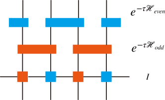
Figure S3: Tensor network representation of the density matrix $\rho(\tau)$ [cf. Eq. (S15)]. The bottom line is the infinite-temperature density operator $\rho(0)=I$. The above blue/red blocks indicate the Trotter gates on even/odd bonds.

D Quantum Many-body Calculation Methods

In this section, we introduce the basic idea of some quantum many-body calculation methods, including exact diagonalization (ED) and linearized tensor renormalization group algorithm (LTRG) Li et al. (2011); Dong et al. (2017). To calculate the thermodynamic properties of a quantum many-body systems, one needs to obtain the partition function $\mathcal{Z}=\mathrm{tr}(\hat{\rho})=\mathrm{tr}(e^{-\beta\mathcal{H}})$ with high precision. For quantum lattice models with $d$-dimension local Hilbert space ($d=2$ for spin-1/2 systems), the $\mathcal{N}$-site many-body basis totally takes a $d^{\mathcal{N}}$-dimension space, and rendering the Hamiltonian $\mathcal{H}$ being a $d^{\mathcal{N}}\times d^{\mathcal{N}}$ matrix.

Limited by the numerical resources, currently one can only store and diagonalize a spin-1/2 Hamiltonian with size of $\mathcal{N}\lesssim 20$ sites. For those small systems, we diagonalize $\mathcal{H}$ by an invertible matrix $\mathcal{U}$ as

$$\mathcal{H}=\mathcal{U}\mathcal{D}\mathcal{U}^{-1}$$ (S10)

with $\mathcal{D}$ diagonalized. Thereafter, we obtain the density matrix of the system at the inverse temperature $\beta$

$$\rho=e^{-\beta\mathcal{H}}=\mathcal{U}\,e^{-\beta\mathcal{D}}\,\mathcal{U}^{-1},$$ (S11)

the partition function

$$\mathcal{Z}=\text{tr}(e^{-\beta\mathcal{H}})=\text{tr}(e^{-\beta\mathcal{D}}),$$ (S12)

and thus other thermodynamic quantities.

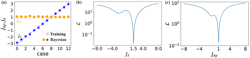
Figure S4: (a) The optimal parameter found after 150 Bayesian optimization iterations. Dashed line indicate the training data, the stars and dots mark respectively the determined parameters $J_{z}$ and $J_{xy}$. (b) A cross cut of the 2D landscape $\mathcal{L}$ in Fig. 2 of the main text, $\mathcal{L}(1.025,J_{z})$ vs. $J_{z}$, with $J_{xy}=1.025$ fixed at the predicted optimal value. (c) shows the cross cut of the 2D landscape $\mathcal{L}$ in Fig. 2, $\mathcal{L}(J_{xy},1.49)$ vs. $J_{xy}$, with a fixed $J_{z}=1.49$ at its predicted optimal value. A sharp deep near the optimal parameter point can be clearly observed in both (b) and (c) panels.

For larger system sizes, we resort to thermal tensor network methods, to be specific, LTRG in this work. The basic idea of LTRG is to, firstly slice the lower-temperature density matrix $\rho(\beta)=e^{-\beta\mathcal{H}}$ into $N$ small slots $\tau=\beta/N$, i.e.

$$\rho(\beta)=e^{-\beta\mathcal{H}}=(e^{-\tau\mathcal{H}})^{N}.$$ (S13)

For a one-dimensional system that contains only the nearest-neighboring interactions, the Hamiltonian can be divided into odd and even parts such that

$$\mathcal{H}=\mathcal{H}_{odd}+\mathcal{H}_{even}.$$ (S14)

Generally, these two parts are non-commutative, so we need to use Trotter-Suzuki decomposition to separate the two terms as

$$\rho(\tau)=e^{-\tau(\mathcal{H}_{odd}+\mathcal{H}_{even})}=e^{-\tau\mathcal{H}_{odd}}e^{-\tau\mathcal{H}_{even}}+O(\tau^{2}).$$ (S15)

Now we arrive at

$$\rho(\beta)=[\rho(\tau)]^{N}\simeq(e^{-\tau\mathcal{H}_{even}}e^{-\tau\mathcal{H}_{odd}})^{N}$$ (S16)

with discretization error $O(\tau^{2})$. The tensor network representation of $\rho(\tau)$ is shown in Fig. S3, with an infinite-temperature density matrix (identity matrix) $\rho(0)=I$ explicitly shown. Therefore, Eq. (S16) can be viewed as a cooling process following a linear temperature gird, i.e. $0\to\tau\to 2\tau\to 3\tau\to\cdots\to N\tau\equiv\beta$. The partition function $\mathcal{Z}=\mathrm{tr}[\rho(\beta)]$ can thus be obtained by fully contracting the tensor network Eq. (S16), and the relevant thermodynamic quantities can be obtained directly from the partition function as,

$$f=-\frac{1}{\beta}\text{ln}\mathcal{Z}$$ (S17)

$$C=\beta^{2}\frac{\partial^{2}\text{ln}\mathcal{Z}}{\partial\beta^{2}}$$ (S18)

$$M=-\frac{\partial f}{\partial h}$$ (S19)

$$\chi=\frac{M}{h}$$ (S20)

where $f$ is the free energy, $C$ is the heat capacity, $h$ is the magnetic field strength, $M$ is the magnetization, and $\chi$ is the magnetic susceptibility.

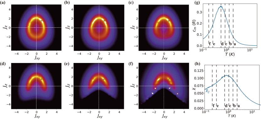
Figure S5: (a-f) Landscape $\mathcal{L}$ interpolated by a grid search of a $30\times 30$ grid with varying cut-off temperature $T_{\rm cut}$, as shown in (g, h). Inconsistent points in (f) are due to interpolation errors. (g, h) indicate the fitted thermodynamic quantities and various $T_{\rm cut}$ values, above which the thermodynamics data are used for fitting.

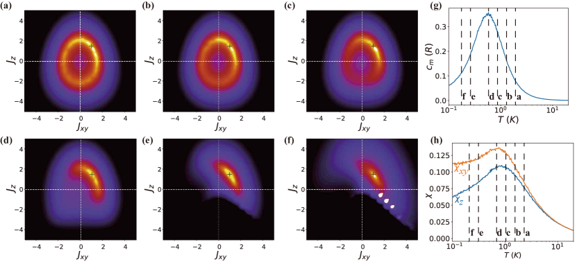
Figure S6: Same layout as Fig. S5, with $\chi_{xy}$ included in the automatic parameter searching.

E More Results on the XXZ HAFC systems

With the training data from the given XXZ spin-chain model, here we show more cases to further validate the robustness of our method. For clarity, the ED calculation of 10 sites XXZ spin chain is used as a rudimentary many-body solver, although in practice we find ED calculations with 8-12 sites lead to virtually the same performance. In Fig. S4, we choose different $J_{z}$ $\in[-3,3]$ and a fixed $J_{xy}=1$, and find that the Bayesian optimization can always refind the correct parameters in all cases and thus constitutes a robust approach.

Then we show the landscapes obtained at different $T_{\rm cut}$ temperatures, fitting jointly the specific heat $C_{m}$ and susceptibility $\chi_{z}$, and observed various landscapes in Fig. S5. We observe a symmetric landscape on $J_{xy}$, due to the identical energy spectra, as well as thermodynamics $C_{m}$ and $\chi_{xy}$, for two models with $\pm|J_{xy}|$. By introducing the in-plane susceptibility $\chi_{xy}$, we can lift this degeneracy, as shown in Fig. S6.

Notably, we find that for a rather high $T_{\rm cut}$, an oval ring with $J_{x}^{2}+J_{y}^{2}+J_{z}^{2}=const.$ lights up in Fig. S5 (a-c). This can be understood, as the high temperature expansion of $C_{m}$ only depends on the squared sum of spin XXZ interactions. As $T_{\rm cut}$ further moves to lower temperatures, the oval ring gradually breaks and eventually converges to two [Fig. S5(d-f)] or one [Fig. S6(d-f)] bright points, depending on whether $\chi_{xy}$ data are included or not. From these panels, we also see that the fittings, although using only small-size ED results, are rather robust as the parameter points found are rather stable as $T_{\rm cut}$ moves to lower temperatures.

F TMGO fitting results

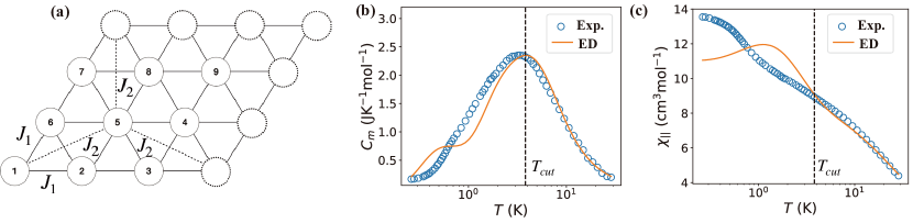
Figure S7: (a) The 9-site triangular lattice with both NN and NNN interactions, and PBC on both directions. (b) Experiment data of the TMGO specific heat and ED fitting with optimal parameter found ($J_{1}=11.57$ K $J_{2}=0.89$ K, $\Delta=5.32$ K, and $g=13.64$). (c) Experiment data of susceptibility and ED fitting with the same parameter.

A 9-site PBC ED calculation is used for fitting [c.f. Fig. S7] (a), and $T_{cut}$ is set to the peak of specific heat $C_{m}$. Both $C_{m}$ and $\chi_{||}$ are used for fitting, and the ED results with the optimal parameter are shown in Fig. S7 (b, c).

References

- Anderson (1973) P. W. Anderson, “Resonating valence bonds: A new kind of insulator?” Mater. Res. Bull. 8, 153 – 160 (1973).
- Kitaev (2006) A. Kitaev, “Anyons in an exactly solved model and beyond,” Ann. Phys. 321, 2 – 111 (2006), January Special Issue.
- Zhou et al. (2017) Y. Zhou, K. Kanoda, and T.-K. Ng, “Quantum spin liquid states,” Rev. Mod. Phys. 89, 025003 (2017).
- Balents (2010) L. Balents, “Spin liquids in frustrated magnets,” Nature (London) 464, 199–208 (2010).
- Han et al. (2012) T. H. Han, J. S. Helton, S. Chu, D. G. Nocera, J. A. Rodriguez-Rivera, C. Broholm, and Y. S. Lee, “Fractionalized excitations in the spin-liquid state of a kagome-lattice antiferromagnet,” Nature 492, 406–410 (2012).
- Fu et al. (2015) Mingxuan Fu, Takashi Imai, Tian-Heng Han, and Young S. Lee, “Evidence for a gapped spin-liquid ground state in a kagome Heisenberg antiferromagnet,” Science 350, 655–658 (2015).
- Shimizu et al. (2003) Y. Shimizu, K. Miyagawa, K. Kanoda, M. Maesato, and G. Saito, “Spin liquid state in an organic Mott insulator with a triangular lattice,” Phys. Rev. Lett. 91, 107001 (2003).
- Yamashita et al. (2010) M. Yamashita, N. Nakata, Y. Senshu, M. Nagata, H. M. Yamamoto, R. Kato, T. Shibauchi, and Y. Matsuda, “Highly mobile gapless excitations in a two-dimensional candidate quantum spin liquid,” Science 328, 1246 (2010).
- Liu et al. (2018) Weiwei Liu, Zheng Zhang, Jianting Ji, Yixuan Liu, Jianshu Li, Xiaoqun Wang, Hechang Lei, Gang Chen, and Qingming Zhang, “Rare-earth chalcogenides: A large family of triangular lattice spin liquid candidates,” Chinese Physics Letters 35, 117501 (2018).
- Jackeli and Khaliullin (2009) G. Jackeli and G. Khaliullin, “Mott insulators in the strong spin-orbit coupling limit: From Heisenberg to a quantum compass and Kitaev models,” Phys. Rev. Lett. 102, 017205 (2009).
- Chaloupka et al. (2010) J. Chaloupka, G. Jackeli, and G. Khaliullin, “Kitaev-Heisenberg model on a honeycomb lattice: Possible exotic phases in iridium oxides ,” Phys. Rev. Lett. 105, 027204 (2010).
- Ye et al. (2012) F. Ye, S. Chi, H. Cao, B. C. Chakoumakos, J. A. Fernandez-Baca, R. Custelcean, T. F. Qi, O. B. Korneta, and G. Cao, “Direct evidence of a zigzag spin-chain structure in the honeycomb lattice: A neutron and X-ray diffraction investigation of single-crystal Na2IrO3,” Phys. Rev. B 85, 180403 (2012).
- Banerjee et al. (2017) A. Banerjee, J. Yan, J. Knolle, C. A. Bridges, M. B. Stone, M. D. Lumsden, D. G. Mandrus, D. A. Tennant, R. Moessner, and S. E. Nagler, “Neutron scattering in the proximate quantum spin liquid -RuCl3,” Science 356, 1055–1059 (2017).
- Laurell and Okamoto (2020) Pontus Laurell and Satoshi Okamoto, “Dynamical and thermal magnetic properties of the Kitaev spin liquid candidate -RuCl3,” npj Quantum Materials 5, 2 (2020).
- Bursill et al. (1996) R. J. Bursill, T. Xiang, and G. A. Gehring, “The density matrix renormalization group for a quantum spin chain at non-zero temperature,” J. Phys. Condens. 8, L583 (1996).
- Wang and Xiang (1997) X. Wang and T. Xiang, “Transfer-matrix density-matrix renormalization-group theory for thermodynamics of one-dimensional quantum systems,” Phys. Rev. B 56, 5061–5064 (1997).
- Xiang (1998) T. Xiang, “Thermodynamics of quantum Heisenberg spin chains,” Phys. Rev. B 58, 9142–9149 (1998).
- Feiguin and White (2005) A. E. Feiguin and S. R. White, “Finite-temperature density matrix renormalization using an enlarged Hilbert space,” Phys. Rev. B 72, 220401(R) (2005).
- White (2009) S. R. White, “Minimally entangled typical quantum states at finite temperature,” Phys. Rev. Lett. 102, 190601 (2009).
- Stoudenmire and White (2010) E. M. Stoudenmire and S. R. White, “Minimally entangled typical thermal state algorithms,” New J. Phys. 12, 055026 (2010).
- Li et al. (2011) W. Li, S.-J. Ran, S.-S. Gong, Y. Zhao, B. Xi, F. Ye, and G. Su, “Linearized tensor renormalization group algorithm for the calculation of thermodynamic properties of quantum lattice models,” Phys. Rev. Lett. 106, 127202 (2011).
- Dong et al. (2017) Y.-L. Dong, L. Chen, Y.-J. Liu, and W. Li, “Bilayer linearized tensor renormalization group approach for thermal tensor networks,” Phys. Rev. B 95, 144428 (2017).
- Chen et al. (2017) B.-B. Chen, Y.-J. Liu, Z. Chen, and W. Li, “Series-expansion thermal tensor network approach for quantum lattice models,” Phys. Rev. B 95, 161104(R) (2017).
- Chen et al. (2018) B.-B. Chen, L. Chen, Z. Chen, W. Li, and A. Weichselbaum, “Exponential thermal tensor network approach for quantum lattice models,” Phys. Rev. X 8, 031082 (2018).
- Li et al. (2019) H. Li, B.-B. Chen, Z. Chen, J. von Delft, A. Weichselbaum, and W. Li, “Thermal tensor renormalization group simulations of square-lattice quantum spin models,” Phys. Rev. B 100, 045110 (2019).
- Carleo and Troyer (2017) G. Carleo and M. Troyer, “Solving the quantum many-body problem with artificial neural networks,” Science 355, 602–606 (2017).
- Liao et al. (2019) H.-J. Liao, J.-G. Liu, L. Wang, and T. Xiang, “Differentiable programming tensor networks,” Phys. Rev. X 9, 031041 (2019).
- Chen et al. (2020) Bin-Bin Chen, Yuan Gao, Yi-Bin Guo, Yuzhi Liu, Hui-Hai Zhao, Hai-Jun Liao, Lei Wang, Tao Xiang, Wei Li, and Z. Y. Xie, “Automatic differentiation for second renormalization of tensor networks,” Phys. Rev. B 101, 220409 (2020).
- Stoudenmire and Schwab (2016) E. Stoudenmire and D. J. Schwab, “Supervised learning with tensor networks,” in Advances in Neural Information Processing Systems 29, edited by D. D. Lee, M. Sugiyama, U. V. Luxburg, I. Guyon, and R. Garnett (Curran Associates, Inc., 2016) pp. 4799–4807.
- Liu et al. (2019) Ding Liu, Shi-Ju Ran, Peter Wittek, Cheng Peng, Raul Blázquez García, Gang Su, and Maciej Lewenstein, “Machine learning by unitary tensor network of hierarchical tree structure,” New Journal of Physics 21, 073059 (2019).
- Ran (2020) Shi-Ju Ran, “Bayesian tensor network with polynomial complexity for probabilistic machine learning,” (2020), arXiv:1912.12923 [stat.ML] .
- Cichocki et al. (2017) Andrzej Cichocki, Anh-Huy Phan, Qibin Zhao, Namgil Lee, Ivan Oseledets, Masashi Sugiyama, and Danilo P. Mandic, “Tensor networks for dimensionality reduction and large-scale optimization: Part 2 applications and future perspectives,” Foundations and Trends® in Machine Learning 9, 431–673 (2017).
- Han et al. (2018) Zhao-Yu Han, Jun Wang, Heng Fan, Lei Wang, and Pan Zhang, “Unsupervised generative modeling using matrix product states,” Phys. Rev. X 8, 031012 (2018).
- Glasser et al. (2019) I. Glasser, R. Sweke, Nicola Pancotti, J. Eisert, and J. I. Cirac, “Expressive power of tensor-network factorizations for probabilistic modeling, with applications from hidden Markov models to quantum machine learning,” in NeurIPS (2019).
- Czarnik and Dziarmaga (2014) P. Czarnik and J. Dziarmaga, “Fermionic projected entangled pair states at finite temperature,” Phys. Rev. B 90, 035144 (2014).
- Note (1) In practice, we first employed a loss function without the denominator in Figs. 2 and 3, and then follows the exact form as Eq. (1) in the cases of Figs. 4 and 5. Both schemes work well, and the design of the loss function have an empirical impact on its overall shape over the parameter space , whose effects in the optimization efficiency will be carefully addressed in future studies.
- LeCun et al. (2015) Yann LeCun, Yoshua Bengio, and Geoffrey Hinton, “Deep learning,” Nature 521, 436–444 (2015).
- Shahriari et al. (2016) B. Shahriari, K. Swersky, Z. Wang, R. P. Adams, and N. de Freitas, “Taking the human out of the loop: A review of Bayesian optimization,” Proceedings of the IEEE 104, 148–175 (2016).
- Melnikov et al. (2018) Alexey A. Melnikov, Hendrik Poulsen Nautrup, Mario Krenn, Vedran Dunjko, Markus Tiersch, Anton Zeilinger, and Hans J. Briegel, “Active learning machine learns to create new quantum experiments,” Proceedings of the National Academy of Sciences 115, 1221–1226 (2018).
- van Tol et al. (1971) M. W. van Tol, L. S. J. M. Henkens, and N. J. Poulis, “High-field magnetic phase transition in ,” Phys. Rev. Lett. 27, 739–741 (1971).
- Xu et al. (2000) Guangyong Xu, C. Broholm, Daniel H. Reich, and M. A. Adams, “Triplet waves in a quantum spin liquid,” Phys. Rev. Lett. 84, 4465–4468 (2000).
- Xiang et al. (2017) Jun-Sen Xiang, Cong Chen, Wei Li, Xian-Lei Sheng, Na Su, Zhao-Hua Cheng, Qiang Chen, and Zi-Yu Chen, “Criticality-enhanced magnetocaloric effect in quantum spin chain material copper nitrate,” Scientific Reports 7, 44643 (2017).
- Berger et al. (1963) L. Berger, S. A. Friedberg, and J. T. Schriempf, “Magnetic susceptibility of Cu ·2.5O at low temperature,” Phys. Rev. 132, 1057–1061 (1963).
- Li et al. (2020a) Han Li, Yuan Da Liao, Bin-Bin Chen, Xu-Tao Zeng, Xian-Lei Sheng, Yang Qi, Zi Yang Meng, and Wei Li, “Kosterlitz-Thouless melting of magnetic order in the triangular quantum Ising material TmMgGaO4,” Nat. Commun. 11, 1111 (2020a).
- Li et al. (2020b) Y. Li, S. Bachus, H. Deng, W. Schmidt, H. Thoma, V. Hutanu, Y. Tokiwa, A. A. Tsirlin, and P. Gegenwart, “Partial up-up-down order with the continuously distributed order parameter in the triangular antiferromagnet ,” Phys. Rev. X 10, 011007 (2020b).
- Shen et al. (2019) Y. Shen, C. Liu, Y. Qin, S. Shen, Y.-D. Li, R. Bewley, A. Schneidewind, G. Chen, and J. Zhao, “Intertwined dipolar and multipolar order in the triangular-lattice magnet TmMgGaO4,” Nat. Commun. 10, 4530 (2019).
- Cevallos et al. (2018) F. A. Cevallos, K. Stolze, T. Kong, and R. J. Cava, “Anisotropic magnetic properties of the triangular plane lattice material TmMgGaO4,” Mater. Res. Bull. 105, 154–158 (2018).
- Hu et al. (2020) Ze Hu, Zhen Ma, Yuan-Da Liao, Han Li, Chunsheng Ma, Yi Cui, Yanyan Shangguan, Zhentao Huang, Yang Qi, Wei Li, Zi Yang Meng, Jinsheng Wen, and Weiqiang Yu, “Evidence of the Berezinskii-Kosterlitz-Thouless phase in a frustrated magnet,” Nature Communications 11, 5631 (2020).
- Zhang et al. (2020) Zheng Zhang, Jianshu Li, Weiwei Liu, Zhitao Zhang, Jianting Ji, Feng Jin, Rui Chen, Junfeng Wang, Xiaoqun Wang, Jie Ma, and Qingming Zhang, “Effective magnetic Hamiltonian at finite temperatures for rare earth chalcogenides,” (2020), arXiv:2011.06274 [cond-mat.str-el] .
- Zhitomirsky (2003) M. E. Zhitomirsky, “Enhanced magnetocaloric effect in frustrated magnets,” Phys. Rev. B 67, 104421 (2003).
- Zhitomirsky and Honecker (2004) M E Zhitomirsky and A Honecker, “Magnetocaloric effect in one-dimensional antiferromagnets,” Journal of Statistical Mechanics: Theory and Experiment 2004, P07012 (2004).
- Garst and Rosch (2005) Markus Garst and Achim Rosch, “Sign change of the grüneisen parameter and magnetocaloric effect near quantum critical points,” Phys. Rev. B 72, 205129 (2005).
- Wolf et al. (2011) Bernd Wolf, Yeekin Tsui, Deepshikha Jaiswal-Nagar, Ulrich Tutsch, Andreas Honecker, Katarina Remović-Langer, Georg Hofmann, Andrey Prokofiev, Wolf Assmus, Guido Donath, and Michael Lang, “Magnetocaloric effect and magnetic cooling near a field-induced quantum-critical point,” Proceedings of the National Academy of Sciences 108, 6862–6866 (2011).
- Gegenwart (2016) Philipp Gegenwart, “Grüneisen parameter studies on heavy fermion quantum criticality,” Reports on Progress in Physics 79, 114502 (2016), arXiv:1608.04907 [cond-mat.str-el] .
- Karbach and Stolze (2005) Peter Karbach and Joachim Stolze, “Spin chains as perfect quantum state mirrors,” Phys. Rev. A 72, 030301 (2005).
- Cappellaro et al. (2007) P. Cappellaro, C. Ramanathan, and D. G. Cory, “Simulations of information transport in spin chains,” Phys. Rev. Lett. 99, 250506 (2007).
- Paszke et al. (2019) Adam Paszke, Sam Gross, Francisco Massa, Adam Lerer, James Bradbury, Gregory Chanan, Trevor Killeen, Zeming Lin, Natalia Gimelshein, Luca Antiga, Alban Desmaison, Andreas Kopf, Edward Yang, Zachary DeVito, Martin Raison, Alykhan Tejani, Sasank Chilamkurthy, Benoit Steiner, Lu Fang, Junjie Bai, and Soumith Chintala, “Pytorch: An imperative style, high-performance deep learning library,” in Advances in Neural Information Processing Systems 32, edited by H. Wallach, H. Larochelle, A. Beygelzimer, F. d'Alché-Buc, E. Fox, and R. Garnett (Curran Associates, Inc., 2019) pp. 8024–8035.
- Lizotte (2008) Daniel James Lizotte, Practical Bayesian Optimization, Ph.D. thesis, CAN (2008), aAINR46365.
- Nogueira (2014–) Fernando Nogueira, “Bayesian Optimization: Open source constrained global optimization tool for Python,” (2014–).
- (60) In Supplementary Materials, we summarize three algorithms adopted in our Hamiltonian searching in Sec. A. Automatic differentiation and Bayesian optimization are briefly recapitulated in Sec. B and Sec. C respectively. We also revisit the basic idea of quantum many-body methods used in this work in Sec. D. More fitting data on the XXZ HAFC and TMGO systems are presented in Sec. E and Sec. F.