An AUK-based index for measuring and testing the joint dependence of a random vector

  Abstract. We present an index of dependence that allows one to measure the joint or mutual dependence of a $d$-dimensional random vector with $d>2$. The index is based on a $d$-dimensional Kendall process. We further propose a standardized version of our index of dependence that is easy to interpret, and provide an algorithm for its computation. We discuss tests of total independence based on consistent estimates of the area under the Kendall curve. We evaluate the performance of our procedures via simulation, and apply our methods to a real data set.
MSC 2010 subject classifications: Primary 62H20, 62H05, 62E10; secondary 62-09, 62G99.
Key words and phrases: Copulas; Dependence axioms; Index of dependence; Kendall-function/plot; Measure of association/dependence; Structure theory; Testing complete independence.

 

1.   Introduction and Literature Review

Advances in technology allow the generation and collection of very large data sets, where the dependencies among the different variables that comprise these data sets are often of considerable interest. In this paper, we consider ways to measure joint or mutual dependence among the components of a $d$-dimensional random vector and to construct test procedures for mutual or total independence.

There is substantial literature on the construction of indices of dependence between two random variables. These include the relevant concept of correlation, for example Pearson (1895) and Spearman’s rho (1904). More recently, Székely et al. (2007) and Székely and Rizzo (2009, 2014) proposed the concept of distance correlation, that represents one of the most important breakthroughs in measuring dependence between two random vectors. Furthermore, a generalization of the concept of distance correlation was recently proposed by Shen et al. (2020). Other proposals include a projection correlation (Zhu et al., 2017; Bergsma and Dassios, 2014; Genest et al., 2019).

We propose an index of dependence that is based on the area under the Kendall curve, generalizing work by Vexler et al. (2019) from the two-dimensional to the $d$-dimensional case. The proposed index measures the dependence between the $d$ components of a random vector. We then construct a test of total independence based on the estimated area under the Kendall curve. This task is different from the task of testing pairwise independence in a collection of random variables.

The literature in statistics includes a few nonparametric procedures to test mutual or joint dependence. These include Simon (1977) who proposed a nonparametric test based on Kendall’s tau. Other tests include Kankainen (1995) and Karvanen (2005). The later author developed a restamping test for testing total independence that is based on the test proposed by Kankainen, for the case of stationary time series.

Pfister et al. (2018) investigated also the problem of testing mutual or joint independence and proposed tests based on the $d$-variable Hilbert-Schmidt independence criterion, dHSIC, thereby extending Kankainen (1995) to the flexible framework of kernel methods. These authors developed their test based on the idea of probability embeddings of marginals and the joint distribution of the random vector $\boldsymbol{X}$.

Our contribution is two-fold. First, we propose n algorithm to construct an index of dependence that is based on the Euclidean distance between the vector of appropriately defined areas under the Kendall curve and the $d$-dimensional vector with components equal to $1/2$. We also present the standardized version of our index of dependence that is easily interpretable, and we note that these indices are copula-based.

Next, we propose a practical, fast to compute test of mutual independence that is also based on the estimate of the area under the Kendall curve. We discuss the asymptotic distribution of our test statistic under the null hypothesis of mutual independence and investigate the performance characteristics of our test via simulation. Furthermore, we provide comparisons with the dHSIC test. The results of our study show that the proposed testing procedure is practical and easily computable — the computation time required to carry out our test is considerably less than the time required to compute the corresponding dHSIC test. Furthermore, the newly proposed test outperforms in terms of power the dHSIC test in smaller samples and performs as the dHSIC test in large samples. The power results apply to all distributions from where samples were generated with the exception of the distributions $U\{C(0,1)\}$ and spiral 1 and 3 distributions.

The paper is organized as follows. Section 2 offers motivation for constructing the index of dependence and presents discussion on appropriate axioms that a measure of dependence must satisfy. Section 3 briefly presents the bivariate case, while Section 4 extends the index to the case where the dimension $d$ is greater than 2. This section also offers an algorithm for the computation of a standardized version of our index. Section 5 proves that the proposed index satisfies the axioms a function must satisfy in order to be a measure of dependence, while Section 6 discuss the estimation of the area under the Kendal curve and the two indices of dependence. Section 7 introduces the test of mutual independence, while Sections 8 and 9 present simulation results and a real data example. Section 10 concludes with a short summary and discussion of the results. Proofs of all relevant theorems are given in the appendix.

2.   Motivation, Notation and Dependence Axioms

Let $X_{1},\ldots,X_{d}$ be a set of $d$ unidimensional random variables (rvs). Let $d_{1}$ and $d_{2}$ be two positive integers such that $d_{1}+d_{2}=d$; consider a partitioning of $X$s into two sets of dimensions $d_{1}$ and $d_{2}$, say $X_{1},\ldots,X_{d_{1}}$ and $X_{d_{1}+1},\ldots,X_{d}$. Consider the random vectors $\boldsymbol{X}_{1}=(X_{1},\ldots,X_{d_{1}})^{T}$, $\boldsymbol{X}_{2}=(X_{d_{1}+1},\ldots,X_{d})^{T}$ and $\boldsymbol{X}=(\boldsymbol{X}_{1}^{T},\boldsymbol{X}_{2}^{T})^{T}=(X_{1},\ldots,X_{d})^{T}$ of dimension $d_{1}$, $d_{2}$ and $d$ respectively. The cumulative distribution functions (cdfs) of $X_{j}$, $\boldsymbol{X}_{1}$, $\boldsymbol{X}_{2}$ and $\boldsymbol{X}$ are denoted by $F_{j}$, $F_{\mathbf{1}}$, $F_{\mathbf{2}}$ and $F$ respectively. Hereafter, we denote $\boldsymbol{x}_{1}=(x_{1},\ldots,x_{d_{1}})^{T}\in\mathds{R}^{d_{1}}$, $\boldsymbol{x}_{2}=(x_{d_{1}+1},\ldots,x_{d})^{T}\in\mathds{R}^{d_{2}}$ and $\boldsymbol{x}=(x_{1},\ldots,x_{d})^{T}\in\mathds{R}^{d}$ being the corresponding realizations of $\boldsymbol{X}_{1}$, $\boldsymbol{X}_{2}$ and $\boldsymbol{X}$. Also, whenever we say that $\boldsymbol{X}$ (or $F$) is a continuous random vector (or cdf) on $\mathds{R}^{d}$ we mean that it has continuous marginal distributions — that do not necessarily have a density function. Hence, we define the next class of random vectors

$$\mathcal{X}^{d}_{0}\doteq\{\boldsymbol{X}\colon\boldsymbol{X}\textrm{ is a continuous random vector on }\mathds{R}^{d}\}.$$

Suppose $\boldsymbol{X}\in\mathcal{X}^{d}_{0}$ and assume that we are interested in measuring the following two kinds of dependence, measured as distances between appropriate cdfs:

1. measuring the distance between $F(\boldsymbol{x})$ and $F_{\mathbf{1}}(\boldsymbol{x}_{1})F_{\mathbf{2}}(\boldsymbol{x}_{2})$;

2. measuring the distance between $F(\boldsymbol{x})$ and $\prod_{j=1}^{d}F_{j}(x_{j})$.

In other words, in $\mathcal{D}_{1}$ we are interested in measuring the pairwise-dependence between $\boldsymbol{X}_{1}$ and $\boldsymbol{X}_{2}$; while in $\mathcal{D}_{2}$ we are interested in measuring the dependence structure of the joint distribution function of $\boldsymbol{X}$. Thus, in $\mathcal{D}_{2}$ we aim to measure joint or mutual dependence. In the bivariate case, i.e. $d=2$ and so $d_{1}=d_{2}=1$, the statements $\mathcal{D}_{1}$ and $\mathcal{D}_{2}$ are identical; while these differ from one another when $d>2$.

We focus in the multivariate case where $d>2$. Consider the rvs $U_{j}$, $j=1,\ldots,d$, independent and identically distributed from $U(0,1)$ such that $\boldsymbol{X}$ and $U_{j}$s are independent, and define the rvs

$$T\doteq F(\boldsymbol{X});\quad\varPi\doteq U_{1}\cdots U_{d};\quad E\doteq-\ln\varPi.$$ (2.1)

Let the components of a random vector $\boldsymbol{X}$ be standardized (each marginal distribution has zero mean and variance one), and denote its variance/covariance matrix by ${\mathrel{\mathchoice{\ooalign{$\displaystyle\mathbf{\Sigma}$\cr\hfil$\displaystyle|$\hfil\cr}}{\ooalign{$\textstyle\mathbf{\Sigma}$\cr\hfil$\textstyle|$\hfil\cr}}{\ooalign{$\scriptstyle\mathbf{\Sigma}$\cr\hfil$\scriptstyle|$\hfil\cr}}{\ooalign{$\scriptscriptstyle\mathbf{\Sigma}$\cr\hfil$\scriptscriptstyle|$\hfil\cr}}}}_{d}(\boldsymbol{\rho})$ with $\boldsymbol{\rho}=(\rho_{ij})\in\mathds{R}^{n(n-1)/2}$, $1\leq i<j\leq d$, that is

$${\mathrel{\mathchoice{\ooalign{$\displaystyle\mathbf{\Sigma}$\cr\hfil$\displaystyle|$\hfil\cr}}{\ooalign{$\textstyle\mathbf{\Sigma}$\cr\hfil$\textstyle|$\hfil\cr}}{\ooalign{$\scriptstyle\mathbf{\Sigma}$\cr\hfil$\scriptstyle|$\hfil\cr}}{\ooalign{$\scriptscriptstyle\mathbf{\Sigma}$\cr\hfil$\scriptscriptstyle|$\hfil\cr}}}}_{d}(\boldsymbol{\rho})=(\sigma_{ij})_{d\times d}\ \textrm{ with }\sigma_{ii}=1\textrm{ and }\sigma_{ij}=\sigma_{ji}=\rho_{ij}\textrm{ for }i<j.$$ (2.2a)

Specifically, for the cases where $$\rho_{ij}=\rho i<j {\mathrel{\mathchoice{\ooalign{$\displaystyle\mathbf{\Sigma}$\cr\hfil$\displaystyle|$\hfil\cr}}{\ooalign{$\textstyle\mathbf{\Sigma}$\cr\hfil$\textstyle|$\hfil\cr}}{\ooalign{$\scriptstyle\mathbf{\Sigma}$\cr\hfil$\scriptstyle|$\hfil\cr}}{\ooalign{$\scriptscriptstyle\mathbf{\Sigma}$\cr\hfil$\scriptscriptstyle|$\hfil\cr}}}}_{d}(\rho)$$ for all , we denote the variance/covariance matrix by , that is,

$${\mathrel{\mathchoice{\ooalign{$\displaystyle\mathbf{\Sigma}$\cr\hfil$\displaystyle|$\hfil\cr}}{\ooalign{$\textstyle\mathbf{\Sigma}$\cr\hfil$\textstyle|$\hfil\cr}}{\ooalign{$\scriptstyle\mathbf{\Sigma}$\cr\hfil$\scriptstyle|$\hfil\cr}}{\ooalign{$\scriptscriptstyle\mathbf{\Sigma}$\cr\hfil$\scriptscriptstyle|$\hfil\cr}}}}_{d}(\rho)=(\sigma_{ij})_{d\times d}\ \textrm{ with }\sigma_{ii}=1\textrm{ and }\sigma_{ij}=\rho\textrm{ for }i\neq j.$$ (2.2b)

In 1959, Rényi’s fundamental article defined a set of axioms that a measure of dependence for a pair of random variables must satisfy; these axioms have been studied and suitably modified by Schweizer and Wolff (1981), see Axioms $A^{\mathrm{R}}_{1}$ to $A^{\mathrm{R}}_{8}$ in Appendix A. In a recent article, Móri and Székely (2019) propose four natural axioms for dependence measures, see Axioms $A^{\mathrm{MS}}_{1}$ to $A^{\mathrm{MS}}_{4}$ in Appendix A. Rényi’s axioms refer only to the 2-dimensional case; while those of Móri and Székely only refer to the case of the statement in $\mathcal{D}_{1}$. Similar to Móri and Székely (2019), Hofert, Oldford, Prasad and Zhu (2019) establish axioms for dependence measures, that also, in general, refer to the statement in $\mathcal{D}_{1}$. We discuss now a modification of Rényi’s axioms that is suitable for $\mathcal{D}_{2}$.

Let $\mathpzc{X}^{d}\subset\mathcal{X}^{d}_{0}$. According to Rényi, a mapping $\delta\colon\mathpzc{X}^{d}\to[0,1]$ is called a mutual dependence measure on $\mathpzc{X}^{d}$ if

1. $\delta(\boldsymbol{X})$ is defined for any $\boldsymbol{X}\in\mathpzc{X}^{d}$.

2. $\delta(\boldsymbol{X})=\delta(\boldsymbol{X}^{*})$ for any permutation $\boldsymbol{X}^{*}=(X_{i_{1}},\ldots,X_{i_{d}})^{T}$ of $\boldsymbol{X}\in\mathpzc{X}^{d}$.

3. $0\leq\delta(\boldsymbol{X})\leq 1$ for any $\boldsymbol{X}\in\mathpzc{X}^{d}$.

4. $\delta(\boldsymbol{X})=0$ if and only if $X_{1},\ldots,X_{d}$ are independent rvs.

5. For $\boldsymbol{X}\in\mathpzc{X}^{d}$, $\delta(\boldsymbol{X})=1$ if and only if each of the $X_{i}$s is a.s. a strictly monotone function of any other.

6. For $\boldsymbol{X}\in\mathpzc{X}^{d}$, if $f_{i}$ is strictly monotone function a.s. on the range of $X_{i}$ for all $i=1,\ldots,d$, then $\delta\{f(\boldsymbol{X})\}=\delta(\boldsymbol{X})$, where $f(\boldsymbol{X})=(f_{1}(X_{1}),\ldots,f_{d}(X_{d}))^{T}\in\mathpzc{X}^{d}$.

7. If $d=2$ and the joint distribution of $\boldsymbol{X}$ is bivariate normal, with correlation coefficient $\rho$, then $\delta(\boldsymbol{X})$ is a strictly increasing function of $|\rho|$.

8. If $\boldsymbol{X}$ and $\boldsymbol{X}_{n}$, $n=1,2,\ldots$, belong to $\mathpzc{X}^{d}$, and if $\boldsymbol{X}_{n}\rightsquigarrow\boldsymbol{X}$, then $\delta(\boldsymbol{X}_{n})\to\delta(\boldsymbol{X})$.

Remark 2.1.

1. For the case $d=3$, consider the matrix given by (2.2b), i.e. ${\mathrel{\mathchoice{\ooalign{$\displaystyle\mathbf{\Sigma}$\cr\hfil$\displaystyle|$\hfil\cr}}{\ooalign{$\textstyle\mathbf{\Sigma}$\cr\hfil$\textstyle|$\hfil\cr}}{\ooalign{$\scriptstyle\mathbf{\Sigma}$\cr\hfil$\scriptstyle|$\hfil\cr}}{\ooalign{$\scriptscriptstyle\mathbf{\Sigma}$\cr\hfil$\scriptscriptstyle|$\hfil\cr}}}}_{3}(\rho)=\mathopen{}\mathclose{{}\left(\textrm{\tiny\begin{tabular}[]{@{}c@{~~}c@{~~}c@{}}1\hfil~{}~{}&$\rho$\hfil~{}~{}&$\rho$\\[-0.64583pt] $\rho$\hfil~{}~{}&1\hfil~{}~{}&$\rho$\\[-0.64583pt] $\rho$\hfil~{}~{}&$\rho$\hfil~{}~{}&1\end{tabular}}}\right)$. The determinant of this matrix is $\det\mathopen{}\mathclose{{}\left\{{\mathrel{\mathchoice{\ooalign{$\displaystyle\mathbf{\Sigma}$\cr\hfil$\displaystyle|$\hfil\cr}}{\ooalign{$\textstyle\mathbf{\Sigma}$\cr\hfil$\textstyle|$\hfil\cr}}{\ooalign{$\scriptstyle\mathbf{\Sigma}$\cr\hfil$\scriptstyle|$\hfil\cr}}{\ooalign{$\scriptscriptstyle\mathbf{\Sigma}$\cr\hfil$\scriptscriptstyle|$\hfil\cr}}}}_{3}(\rho)}\right\}=(1-\rho)^{2}(1+2\rho)$. Since a variance/covariance matrix is a positive definite matrix and so its determinant is non-negative, it follows that $\rho\geq-1/2$. Consequently, ${\mathrel{\mathchoice{\ooalign{$\displaystyle\mathbf{\Sigma}$\cr\hfil$\displaystyle|$\hfil\cr}}{\ooalign{$\textstyle\mathbf{\Sigma}$\cr\hfil$\textstyle|$\hfil\cr}}{\ooalign{$\scriptstyle\mathbf{\Sigma}$\cr\hfil$\scriptstyle|$\hfil\cr}}{\ooalign{$\scriptscriptstyle\mathbf{\Sigma}$\cr\hfil$\scriptscriptstyle|$\hfil\cr}}}}_{3}(\rho)$ is a variance/covariance matrix if and only if $-1/2\leq\rho\leq 1$. Based on the above analysis, there are positive values of $\rho$ for which the fact that ${\mathrel{\mathchoice{\ooalign{$\displaystyle\mathbf{\Sigma}$\cr\hfil$\displaystyle|$\hfil\cr}}{\ooalign{$\textstyle\mathbf{\Sigma}$\cr\hfil$\textstyle|$\hfil\cr}}{\ooalign{$\scriptstyle\mathbf{\Sigma}$\cr\hfil$\scriptstyle|$\hfil\cr}}{\ooalign{$\scriptscriptstyle\mathbf{\Sigma}$\cr\hfil$\scriptscriptstyle|$\hfil\cr}}}}_{3}(\rho)$ can be assumed as a variance/covariance matrix of a 3-dimensional random vector does not imply that ${\mathrel{\mathchoice{\ooalign{$\displaystyle\mathbf{\Sigma}$\cr\hfil$\displaystyle|$\hfil\cr}}{\ooalign{$\textstyle\mathbf{\Sigma}$\cr\hfil$\textstyle|$\hfil\cr}}{\ooalign{$\scriptstyle\mathbf{\Sigma}$\cr\hfil$\scriptstyle|$\hfil\cr}}{\ooalign{$\scriptscriptstyle\mathbf{\Sigma}$\cr\hfil$\scriptscriptstyle|$\hfil\cr}}}}_{3}(-\rho)$ can also be assumed as a variance/covariance matrix. For example, set $\rho=0.7$; then, ${\mathrel{\mathchoice{\ooalign{$\displaystyle\mathbf{\Sigma}$\cr\hfil$\displaystyle|$\hfil\cr}}{\ooalign{$\textstyle\mathbf{\Sigma}$\cr\hfil$\textstyle|$\hfil\cr}}{\ooalign{$\scriptstyle\mathbf{\Sigma}$\cr\hfil$\scriptstyle|$\hfil\cr}}{\ooalign{$\scriptscriptstyle\mathbf{\Sigma}$\cr\hfil$\scriptscriptstyle|$\hfil\cr}}}}_{3}(0.7)$ is a positive definete $3\times 3$ matrix and hence we can consider the normal distribution $\mathcal{N}_{3}(\mathbf{0},{\mathrel{\mathchoice{\ooalign{$\displaystyle\mathbf{\Sigma}$\cr\hfil$\displaystyle|$\hfil\cr}}{\ooalign{$\textstyle\mathbf{\Sigma}$\cr\hfil$\textstyle|$\hfil\cr}}{\ooalign{$\scriptstyle\mathbf{\Sigma}$\cr\hfil$\scriptstyle|$\hfil\cr}}{\ooalign{$\scriptscriptstyle\mathbf{\Sigma}$\cr\hfil$\scriptscriptstyle|$\hfil\cr}}}}_{d}(0.7))$, while ${\mathrel{\mathchoice{\ooalign{$\displaystyle\mathbf{\Sigma}$\cr\hfil$\displaystyle|$\hfil\cr}}{\ooalign{$\textstyle\mathbf{\Sigma}$\cr\hfil$\textstyle|$\hfil\cr}}{\ooalign{$\scriptstyle\mathbf{\Sigma}$\cr\hfil$\scriptstyle|$\hfil\cr}}{\ooalign{$\scriptscriptstyle\mathbf{\Sigma}$\cr\hfil$\scriptscriptstyle|$\hfil\cr}}}}_{3}(-0.7)$ is not a positive definete matrix and so the notation $\mathcal{N}_{3}(\mathbf{0},{\mathrel{\mathchoice{\ooalign{$\displaystyle\mathbf{\Sigma}$\cr\hfil$\displaystyle|$\hfil\cr}}{\ooalign{$\textstyle\mathbf{\Sigma}$\cr\hfil$\textstyle|$\hfil\cr}}{\ooalign{$\scriptstyle\mathbf{\Sigma}$\cr\hfil$\scriptstyle|$\hfil\cr}}{\ooalign{$\scriptscriptstyle\mathbf{\Sigma}$\cr\hfil$\scriptscriptstyle|$\hfil\cr}}}}_{d}(-0.7))$ makes no sense.

   In general, the determinant of ${\mathrel{\mathchoice{\ooalign{$\displaystyle\mathbf{\Sigma}$\cr\hfil$\displaystyle|$\hfil\cr}}{\ooalign{$\textstyle\mathbf{\Sigma}$\cr\hfil$\textstyle|$\hfil\cr}}{\ooalign{$\scriptstyle\mathbf{\Sigma}$\cr\hfil$\scriptstyle|$\hfil\cr}}{\ooalign{$\scriptscriptstyle\mathbf{\Sigma}$\cr\hfil$\scriptscriptstyle|$\hfil\cr}}}}_{d}(\rho)$, given by (2.2b), is $\det\mathopen{}\mathclose{{}\left\{{\mathrel{\mathchoice{\ooalign{$\displaystyle\mathbf{\Sigma}$\cr\hfil$\displaystyle|$\hfil\cr}}{\ooalign{$\textstyle\mathbf{\Sigma}$\cr\hfil$\textstyle|$\hfil\cr}}{\ooalign{$\scriptstyle\mathbf{\Sigma}$\cr\hfil$\scriptstyle|$\hfil\cr}}{\ooalign{$\scriptscriptstyle\mathbf{\Sigma}$\cr\hfil$\scriptscriptstyle|$\hfil\cr}}}}_{d}(\rho)}\right\}=(1-\rho)^{d-1}\{1+\rho(d-1)\}$. Therefore, this matrix is a variance/covariance matrix if and only if $(1-d)^{-1}\leq\rho\leq 1$. Let $\boldsymbol{X}\sim\mathcal{N}_{d}(\mathbf{0},{\mathrel{\mathchoice{\ooalign{$\displaystyle\mathbf{\Sigma}$\cr\hfil$\displaystyle|$\hfil\cr}}{\ooalign{$\textstyle\mathbf{\Sigma}$\cr\hfil$\textstyle|$\hfil\cr}}{\ooalign{$\scriptstyle\mathbf{\Sigma}$\cr\hfil$\scriptstyle|$\hfil\cr}}{\ooalign{$\scriptscriptstyle\mathbf{\Sigma}$\cr\hfil$\scriptscriptstyle|$\hfil\cr}}}}_{d}(\rho))$; then, the acceptable values of $\rho$ are $(1-d)^{-1}\leq\rho\leq 1$. If Axiom $A^{\mathrm{R}}_{7}$ can be modified for general $d$, then a measure of dependence will take the same value for both $\mathcal{N}_{d}(\mathbf{0},{\mathrel{\mathchoice{\ooalign{$\displaystyle\mathbf{\Sigma}$\cr\hfil$\displaystyle|$\hfil\cr}}{\ooalign{$\textstyle\mathbf{\Sigma}$\cr\hfil$\textstyle|$\hfil\cr}}{\ooalign{$\scriptstyle\mathbf{\Sigma}$\cr\hfil$\scriptstyle|$\hfil\cr}}{\ooalign{$\scriptscriptstyle\mathbf{\Sigma}$\cr\hfil$\scriptscriptstyle|$\hfil\cr}}}}_{d}(\rho))$ and $\mathcal{N}_{d}(\mathbf{0},{\mathrel{\mathchoice{\ooalign{$\displaystyle\mathbf{\Sigma}$\cr\hfil$\displaystyle|$\hfil\cr}}{\ooalign{$\textstyle\mathbf{\Sigma}$\cr\hfil$\textstyle|$\hfil\cr}}{\ooalign{$\scriptstyle\mathbf{\Sigma}$\cr\hfil$\scriptstyle|$\hfil\cr}}{\ooalign{$\scriptscriptstyle\mathbf{\Sigma}$\cr\hfil$\scriptscriptstyle|$\hfil\cr}}}}_{d}(-\rho))$ distributions for all $\rho$-values; on the other hand, for $d>2$ and each $(d-1)^{-1}<\rho\leq 1$ the notation $\mathcal{N}_{d}(\mathbf{0},{\mathrel{\mathchoice{\ooalign{$\displaystyle\mathbf{\Sigma}$\cr\hfil$\displaystyle|$\hfil\cr}}{\ooalign{$\textstyle\mathbf{\Sigma}$\cr\hfil$\textstyle|$\hfil\cr}}{\ooalign{$\scriptstyle\mathbf{\Sigma}$\cr\hfil$\scriptstyle|$\hfil\cr}}{\ooalign{$\scriptscriptstyle\mathbf{\Sigma}$\cr\hfil$\scriptscriptstyle|$\hfil\cr}}}}_{d}(\rho))$ denotes the $d$-dimensional normal distribution with mean vector $\mathbf{0}$ and variance/covariance matrix ${\mathrel{\mathchoice{\ooalign{$\displaystyle\mathbf{\Sigma}$\cr\hfil$\displaystyle|$\hfil\cr}}{\ooalign{$\textstyle\mathbf{\Sigma}$\cr\hfil$\textstyle|$\hfil\cr}}{\ooalign{$\scriptstyle\mathbf{\Sigma}$\cr\hfil$\scriptstyle|$\hfil\cr}}{\ooalign{$\scriptscriptstyle\mathbf{\Sigma}$\cr\hfil$\scriptscriptstyle|$\hfil\cr}}}}_{d}(\rho)$, while the notation $\mathcal{N}_{d}(\mathbf{0},{\mathrel{\mathchoice{\ooalign{$\displaystyle\mathbf{\Sigma}$\cr\hfil$\displaystyle|$\hfil\cr}}{\ooalign{$\textstyle\mathbf{\Sigma}$\cr\hfil$\textstyle|$\hfil\cr}}{\ooalign{$\scriptstyle\mathbf{\Sigma}$\cr\hfil$\scriptstyle|$\hfil\cr}}{\ooalign{$\scriptscriptstyle\mathbf{\Sigma}$\cr\hfil$\scriptscriptstyle|$\hfil\cr}}}}_{d}(-\rho))$ does not correspond to any distribution.

2. One may incorrectly suggest an extension of $A^{\mathrm{R}}_{7}$ as follows. For a $d$-dimensional normal distribution for fixed $\rho_{ij}$ with $(i,j)\neq(i_{0},j_{0})$, a measure of mutual dependence must be an increasing function of $|\rho_{i_{0}j_{0}}|$. To explain why the aforementioned statement is incorrect, we consider the 3-dimensional normal distributions $F\sim\mathcal{N}_{3}(\mathbf{0},{\mathrel{\mathchoice{\ooalign{$\displaystyle\mathbf{\Sigma}$\cr\hfil$\displaystyle|$\hfil\cr}}{\ooalign{$\textstyle\mathbf{\Sigma}$\cr\hfil$\textstyle|$\hfil\cr}}{\ooalign{$\scriptstyle\mathbf{\Sigma}$\cr\hfil$\scriptstyle|$\hfil\cr}}{\ooalign{$\scriptscriptstyle\mathbf{\Sigma}$\cr\hfil$\scriptscriptstyle|$\hfil\cr}}}}_{F})$ and $G\sim\mathcal{N}_{3}(\mathbf{0},{\mathrel{\mathchoice{\ooalign{$\displaystyle\mathbf{\Sigma}$\cr\hfil$\displaystyle|$\hfil\cr}}{\ooalign{$\textstyle\mathbf{\Sigma}$\cr\hfil$\textstyle|$\hfil\cr}}{\ooalign{$\scriptstyle\mathbf{\Sigma}$\cr\hfil$\scriptstyle|$\hfil\cr}}{\ooalign{$\scriptscriptstyle\mathbf{\Sigma}$\cr\hfil$\scriptscriptstyle|$\hfil\cr}}}}_{G})$, where the variance/covariance matrices are ${\mathrel{\mathchoice{\ooalign{$\displaystyle\mathbf{\Sigma}$\cr\hfil$\displaystyle|$\hfil\cr}}{\ooalign{$\textstyle\mathbf{\Sigma}$\cr\hfil$\textstyle|$\hfil\cr}}{\ooalign{$\scriptstyle\mathbf{\Sigma}$\cr\hfil$\scriptstyle|$\hfil\cr}}{\ooalign{$\scriptscriptstyle\mathbf{\Sigma}$\cr\hfil$\scriptscriptstyle|$\hfil\cr}}}}_{F}=\mathopen{}\mathclose{{}\left(\textrm{\tiny\begin{tabular}[]{@{}c@{~~}c@{~~}c@{}}1\hfil~{}~{}&$-0.5$\hfil~{}~{}&$-0.5$\\[-0.64583pt] $-0.5$\hfil~{}~{}&1\hfil~{}~{}&$\phantom{-}0.5$\\[-0.64583pt] $-0.5$\hfil~{}~{}&$\phantom{-}0.5$\hfil~{}~{}&1\end{tabular}}}\right)$ and ${\mathrel{\mathchoice{\ooalign{$\displaystyle\mathbf{\Sigma}$\cr\hfil$\displaystyle|$\hfil\cr}}{\ooalign{$\textstyle\mathbf{\Sigma}$\cr\hfil$\textstyle|$\hfil\cr}}{\ooalign{$\scriptstyle\mathbf{\Sigma}$\cr\hfil$\scriptstyle|$\hfil\cr}}{\ooalign{$\scriptscriptstyle\mathbf{\Sigma}$\cr\hfil$\scriptscriptstyle|$\hfil\cr}}}}_{G}=\mathopen{}\mathclose{{}\left(\textrm{\tiny\begin{tabular}[]{@{}c@{~~}c@{~~}c@{}}1\hfil~{}~{}&$-0.5$\hfil~{}~{}&$-0.5$\\[-0.64583pt] $-0.5$\hfil~{}~{}&1\hfil~{}~{}&$-0.5$\\[-0.64583pt] $-0.5$\hfil~{}~{}&$-0.5$\hfil~{}~{}&1\end{tabular}}}\right)$. Suppose $\boldsymbol{X}\sim G$. Because of $\det({\mathrel{\mathchoice{\ooalign{$\displaystyle\mathbf{\Sigma}$\cr\hfil$\displaystyle|$\hfil\cr}}{\ooalign{$\textstyle\mathbf{\Sigma}$\cr\hfil$\textstyle|$\hfil\cr}}{\ooalign{$\scriptstyle\mathbf{\Sigma}$\cr\hfil$\scriptstyle|$\hfil\cr}}{\ooalign{$\scriptscriptstyle\mathbf{\Sigma}$\cr\hfil$\scriptscriptstyle|$\hfil\cr}}}}_{G})=0$, there is constant vector $\boldsymbol{c}\in\mathds{R}^{3}$ such that $\boldsymbol{c}^{T}\boldsymbol{X}$ is a constant with probability one, that is, $\boldsymbol{X}$ lies on a subset of $\mathds{R}^{3}$ of dimension 2. The support of $F$ is $S_{F}=\mathds{R}^{3}$ while the support of $G$ is $S_{G}\subsetneq\mathds{R}^{3}$ with $\dim(S_{G})=2$. Figures 1(a) and 1(b) present scatterplots based on random samples of size $1000$ from $F$ and $G$ respectively. It is clear that $G$ has a stronger dependence structure than $F$, and so it is an abnormal situation a measure of dependence to have the same value for $F$ and $G$.

3. In view of (a) and (b), such modification of Axiom $A^{\mathrm{R}}_{7}$ makes no sense for dimension $d>2$.

On the other hand, according to the definition by Móri and Székely, a mapping $\delta\colon\mathpzc{X}^{d}\to[0,1]$ is called a structure dependence measure on $\mathpzc{X}^{d}$ if

1. $\delta(\boldsymbol{X})=0$ if and only if $X_{1},\ldots,X_{n}$ are independent rvs.

2. $\delta(\boldsymbol{X})$ is invariant with respect to all similarity transformations of $\mathds{R}^{d}$; that is, $\delta(L\boldsymbol{X})=\delta(\boldsymbol{X})$ where $L$ is similarity transformation of $\mathds{R}^{d}$.

3. $\delta(\boldsymbol{X})=1$ if and only if there is a similarity transformation $L$ such that $L\boldsymbol{X}=(X_{L},\ldots,X_{L})^{T}\in\mathpzc{X}^{d}$ with probability 1.

4. $\delta(\cdot)$ is continuous; that is, if $\boldsymbol{X}$ and $\boldsymbol{X}_{n}$, $n=1,2,\ldots$, belong to $\mathpzc{X}^{d}$ such that $\boldsymbol{X}_{n}$ is uniform integrable and $\boldsymbol{X}_{n}\rightsquigarrow\boldsymbol{X}$, then $\delta(\boldsymbol{X}_{n})\to\delta(\boldsymbol{X})$.

We note that Móri and Székely (2019) as well as Hofert et al. (2019) avoid to establish an axiom analogous to $A^{\mathrm{R}}_{7}$. In Section 5 we prove that our proposed index satisfies both sets of axioms, the modified Rényi ($A_{1}$-$A_{6}$, $A_{8}$) and Móri and Székely ($A^{\prime}_{1}$-$A^{\prime}_{4}$).

3.   The bivariate case

We aim to construct a measure of mutual dependence that satisfies axioms $A_{1}$-$A_{8}$ discussed in the previous section. For this purpose, in this section we briefly discuss the bivariate case that has been studied by Vexler et al. (2019).

Consider the rvs $T$ and $\varPi$ defined by (2.1). The Kendall distribution function is defined as $K(t)=\operatorname{\mathds{P}}(T\leq t)$. Since the distribution function of $\varPi$ that corresponds to the independent case is $K_{\varPi}(t)=t-t\ln t$, $t\in[0,1]$, the Kendall-plot is the visualization of the curve $(K(t),t-t\ln t)$, $t\in[0,1]$, and compared to the diagonal line $(t-t\ln t,t-t\ln t)$, $t\in[0,1]$, it provides a rich source of information reference the association between the components of $\boldsymbol{X}$. In the light of an ROC analysis, Vexler et al. (2019) show that the area under the Kendall curve is $\mathrm{AUK}=-\int_{0}^{1}K(t)\ln t\operatorname{d\textrm{$t$}}$, and then that

$$\mathrm{AUK}=\operatorname{\mathds{E}}(1-T+T\ln T),$$

which is useful both, for direct evaluation and for simulation studies based on the $\mathrm{AUK}$; it is also used for nonparametric estimation of $\mathrm{AUK}$ based on a random sample of pairs from $F$.

Vexler et al. (2019) offer motivation for the use of an extension of the Kendall plot to a multi-panel Kendall plot that consists of the ordinary Kendall plots of the four orthogonal rotations of $\boldsymbol{X}$; in particular, these are the Kendall plots that correspond to the Kendall functions $K_{i}(t)=\operatorname{\mathds{P}}\{H_{i}(\boldsymbol{X})\leq t\}$, $i=1,\ldots,4$, where

$$\begin{split}H_{1}(x_{1},x_{2})&=\operatorname{\mathds{P}}(X_{1}\leq x_{1},X_{2}\leq x_{2}),\quad H_{2}(x_{1},x_{2})=\operatorname{\mathds{P}}(X_{1}>x_{1},X_{2}\leq x_{2}),\\ H_{3}(x_{1},x_{2})&=\operatorname{\mathds{P}}(X_{1}\leq x_{1},X_{2}>x_{2}),\quad H_{4}(x_{1},x_{2})=\operatorname{\mathds{P}}(X_{1}>x_{1},X_{2}>x_{2}).\end{split}$$ (3.1)

Using these Kendall functions, they provide the four corresponding $\mathrm{AUK}$s ($\mathrm{AUK}_{i}$, $i=1,\ldots,4$). Based on $\boldsymbol{D}=(\mathrm{AUK}_{1},\ldots,\mathrm{AUK}_{4})^{T}$ they establish an index of dependence between $X_{1}$ and $X_{2}$ by the relation

$$I=(8/5)^{1/2}\|\boldsymbol{D}-\boldsymbol{\varDelta}\|,$$

where $\boldsymbol{\varDelta}=(1/2,\ldots,1/2)^{T}\in\mathds{R}^{4}$ and $\|\boldsymbol{x}\|$ denotes the Euclidean norm of the vector $\boldsymbol{x}$. They also present a standardized index of dependence based on $I$ that ensures a linear mapping with $|\rho|$ in the case of the bivariate normal distribution, and they give an approximation of this standardized index by

$$I^{*}=\varphi_{2}(I),$$

where $\varphi_{2}(t)=2.070t+0.061t^{2}-2.471t^{3}+1.307t^{4}+0.033t^{5}$, $t\in[0,1]$.

In what follows, we will extend the index of dependence discussed above to the $d$-dimensional case, $d>2$.

4.   Extension to higher dimensional case

Let $\boldsymbol{X}$ be a $d$-dimensional random vector which has continuous components. For the dimension $d$ of $\boldsymbol{X}$, consider the rvs $T$, $\varPi$ and $E$ defined by (2.1). A natural extension from the bivariate case to $d$-dimensional case of the Kendall distribution function is given by $K(t)=\operatorname{\mathds{P}}(T\leq t)$. When we are interested in measuring the dependence structure of $\boldsymbol{X}$, according to $\mathcal{D}_{2}$, we can plot this Kendall function against the cdf of $\varPi$, which corresponds to the case of independence of the components of $\boldsymbol{X}$; and then, we compare this curve with the diagonal line in $[0,1]\times[0,1]$. Namely, we compare the curve $(K(t),K_{\varPi}(t))$ with the diagonal line $(K_{\varPi}(t),K_{\varPi}(t))$, $t\in[0,1]$. Both Kendall cdf, $K_{\varPi}(\cdot)$, and probability density function (pdf), $k_{\varPi}(\cdot)$, of $\varPi$ may by computed in close forms. Specifically, as is evident $E\sim\mathrm{Erlang}(d,1)$,

$$K_{\varPi}(t)=t\sum_{j=0}^{d-1}\frac{(-1)^{k}}{k!}\ln^{k}t\ \ \text{and}\ \ k_{\varPi}(t)=\frac{(-1)^{d-1}}{(d-1)!}\ln^{d-1}t,\quad 0<t<1.$$ (4.1)

Observe now that $2E$ follows the chi-square distribution with $2d$ degrees of freedom, denoted as $E\sim\chi^{2}_{2d}$. By definition of $E$, see (2.1), the cdf and pdf of $\varPi$ can be presented through the cdf and pdf of $\chi^{2}_{2d}$; specifically,

$$K_{\varPi}(t)=1-F_{\chi^{2}_{2d}}(-2\ln t)\ \ \textrm{and}\ \ k_{\varPi}(t)=\frac{2}{t}f_{\chi^{2}_{2d}}(-2\ln t),\quad t>0.$$

The above formulas are appropriate for computation.

The area under the Kendall ($\mathrm{AUK}$) curve is $\int_{0}^{1}K(t)\operatorname{d\textrm{$K_{\varPi}(t)$}}=\int_{0}^{1}K(t)k_{\varPi}(t)\operatorname{d\textrm{$t$}}$, that is

$$\mathrm{AUK}=\operatorname{\mathds{P}}(T\leq\varPi).$$

Since $\operatorname{\mathds{P}}(T\leq\varPi)=\operatorname{\mathds{E}}\{\operatorname{\mathds{P}}(T\leq\varPi|\varPi)\}=\operatorname{\mathds{E}}\{\operatorname{\mathds{P}}(T\leq\varPi|T)\}=\operatorname{\mathds{E}}\{1-\operatorname{\mathds{P}}(\varPi<T|T)\}$,

$$\mathrm{AUK}=\operatorname{\mathds{E}}\mathopen{}\mathclose{{}\left\{K(\varPi)}\right\}=\operatorname{\mathds{E}}\mathopen{}\mathclose{{}\left\{1-K_{\varPi}(T)}\right\}.$$

Note that the formulas of $K_{\varPi}$ and $\mathrm{AUK}$ in bivariate case follow from the above corresponding formulas of the general case by setting $d=2$.

The distance between $\mathrm{AUK}$ and $1/2$ may itself be used as a measure of divergence between $F$ and $\prod_{j=1}^{d}F_{j}$. But, it cannot be used as a measure of dependence because it does not satisfy the axioms of a measure of dependence that are listed in Section 2, Axioms $A_{1}$ to $A_{8}$ or $A^{\prime}_{1}$ to $A^{\prime}_{4}$.

We now investigate the four Kendall functions that lead to this multi-panel plot in the bivariate case. This investigation offers understanding that is used in the extension of the work for the case of $d>2$. Observe that, since $X_{1}$ and $X_{2}$ are continuous, the functions $H_{1},\ldots,H_{4}$ that are defined by (3.1) are the cdfs of $\boldsymbol{X}_{1}=(X_{1},X_{2})^{T}$, $\boldsymbol{X}_{2}=(-X_{1},X_{2})^{T}$, $\boldsymbol{X}_{3}=(-X_{1},-X_{2})^{T}$ and $\boldsymbol{X}_{4}=(X_{1},-X_{2})^{T}$ respectively; hence, the Kendall distribution functions $K_{1},\ldots,K_{4}$ are the corresponding ordinary Kendall distribution functions of $\boldsymbol{X}_{1},\ldots,\boldsymbol{X}_{4}$. Therefore, the four rotations of a bivariate random vector are leading to the construction of the corresponding Kendall functions, and so to the construction of the $\mathrm{AUK}$-vector, $\boldsymbol{D}=(\mathrm{AUK}_{1},\ldots,\mathrm{AUK}_{4})^{T}$, that can be presented in an algebraic way, through all possible multiplications of the components $X_{1}$ and $X_{2}$ with $\pm$. This representation provides us a natural algebraic manner to extend the $\mathrm{AUK}$-method in highest dimensional random vectors.

In view of the above analysis, we consider the set of the orthogonal “rotations” of $\boldsymbol{X}$, say $\mathcal{R}(\boldsymbol{X})$. Analytically, define the subset $\mathds{S}^{d}$ of $\mathds{R}^{d}$ that contains all possible vectors with elements $\pm 1$, that is

$$\mathds{S}^{d}\doteq\{-,+\}^{d}=\{\boldsymbol{s}_{j}\}_{j=1}^{2^{d}}.$$

Then, the set of the orthogonal “rotations” of $\boldsymbol{X}$ is

$$\mathcal{R}(\boldsymbol{X})\doteq\{\boldsymbol{X}_{j}=\operatorname{diag}(\boldsymbol{s}_{j})\boldsymbol{X}\colon\boldsymbol{s}\in\mathds{S}^{d}\},$$

where $\operatorname{diag}(\boldsymbol{s}_{j})$ denotes the $d\times d$ diagonal matrix with diagonal elements the elements of $\boldsymbol{s}_{j}$. For $\boldsymbol{X}_{j}\in\mathcal{R}(\boldsymbol{X})$, $j=1,\ldots,2^{d}$, define

$$T_{j}\doteq F_{\boldsymbol{X}_{j}}(\boldsymbol{X}_{j})\quad\text{and}\quad K_{j}(t)=\operatorname{\mathds{P}}(T_{j}\leq t).$$

The corresponding, under the Kendall curve, areas are

$$\mathrm{AUK}_{j}=\operatorname{\mathds{P}}(T_{j}\leq\varPi)=\operatorname{\mathds{E}}\mathopen{}\mathclose{{}\left\{1-K_{\varPi}(T_{j})}\right\}.$$

Define $\boldsymbol{D}=(\mathrm{AUK}_{1},\ldots,\mathrm{AUK}_{2^{d}})^{T}$ and $\boldsymbol{\varDelta}=(1/2,\ldots,1/2)^{T}\in\mathds{R}^{2^{d}}$.

Let now $X$ be a continuous rv, and consider the random vectors $\boldsymbol{X}_{1}=(X,\ldots,X)^{T}$ and $\boldsymbol{X}_{2}=(X,\ldots,X,-X)^{T}$ in $\mathcal{X}^{d}$. Write $\boldsymbol{X}_{2}=f(\boldsymbol{X}_{1})$, where $f=(f_{1},\ldots,f_{d})^{T}$ with $f_{i}(x)=x$ for $i=1,\ldots,d-1$ and $f_{d}(x)=-x$. Obviously, $f_{i}$ is a strictly monotone function for all $i=1,\ldots,d$, and $f$ is a similarity transformation; so, for any measure of dependence $\delta$ it is required $\delta(\boldsymbol{X}_{1})=\delta(\boldsymbol{X}_{2})$. On the other hand, the Kendall functions of $\boldsymbol{X}_{1}$ and $\boldsymbol{X}_{2}$ are $K_{1}(t)\equiv K_{\boldsymbol{X}_{1}}(t)=t$ and $K_{2}(t)\equiv K_{\boldsymbol{X}_{2}}(t)=1$, $0\leq t\leq 1$. By application of the formula $\mathrm{AUK}=\int_{0}^{1}K(t)k_{\varPi}(t)\operatorname{d\textrm{$t$}}$, we get $\mathrm{AUK}_{1}=2^{-d}$ and $\mathrm{AUK}_{2}=1$ (for computational details see in the proof of (4.2) in Appendix D), and hence, the distances between $\mathrm{AUK}_{\boldsymbol{X}_{i}}$ and $1/2$ (the value that corresponds to the independence case), $i=1,2$, are $1/2-2^{-d}$ and $1/2$ respectively. Because of Axiom $A_{6}$ or Axiom $A^{\prime}_{2}$, the $\mathrm{AUK}$ of $\boldsymbol{X}\in\mathcal{X}^{d}$ cannot be used for measuring the dependence structure of $\boldsymbol{X}$.

In general, due to $A_{6}$ or $A^{\prime}_{2}$, $\delta(\boldsymbol{X}_{j})=\delta(\boldsymbol{X})$ for all $\boldsymbol{X}_{j}\in\mathcal{R}(\boldsymbol{X})$. Hence, we propose an $\mathrm{AUK}$-based index of dependence of the form $c_{d}\|\boldsymbol{D}-\boldsymbol{\varDelta}\|$, where the constant $c_{d}$ is chosen such that the index takes the value 1 whenever $\boldsymbol{X}$ is of the form $(X,\ldots,X)^{T}$ for some continuous rv $X$. Let $X$ be a continuous rv and set $\boldsymbol{X}=(X,\ldots,X)^{T}\in\mathcal{X}^{d}$. Then, the set of random vectors $\mathcal{R}(\boldsymbol{X})$ contains exactly two random vectors with all components being the same, $(X,\ldots,X)^{T}$ and $(-X,\ldots,-X)^{T}$. Each of $2^{d}-2$ remaining random vectors has components that are rvs $X$ and $-X$. Each of $(X,\ldots,X)^{T}$ and $(-X,\ldots,-X)^{T}$ has the same Kendall function $t$, $0\leq t\leq 1$, while each of $2^{d}-2$ remaining random vectors has the same Kendall function $1$, $0\leq t\leq 1$; therefore, the constant $c_{d}$ is (for computational details see in the proof of (4.2) in Appendix D)

$$c_{d}=\mathopen{}\mathclose{{}\left(2^{d-2}-2^{1-d}+2^{1-2d}}\right)^{-1/2}.$$ (4.2)

Thus, the proposed index of dependence takes the form

$$I=\mathopen{}\mathclose{{}\left(2^{d-2}-2^{1-d}+2^{1-2d}}\right)^{-1/2}\|\boldsymbol{D}-\boldsymbol{\varDelta}\|.$$ (4.3)

Similar to the bivariate case, we are interested in finding the easily interpreted standardized index, $I_{\mathrm{st}}$. This index is a function of $I$ that maps $I\mapsto|\rho|$ whenever $\boldsymbol{X}\sim\mathcal{N}_{d}(\mathbf{0},{\mathrel{\mathchoice{\ooalign{$\displaystyle\mathbf{\Sigma}$\cr\hfil$\displaystyle|$\hfil\cr}}{\ooalign{$\textstyle\mathbf{\Sigma}$\cr\hfil$\textstyle|$\hfil\cr}}{\ooalign{$\scriptstyle\mathbf{\Sigma}$\cr\hfil$\scriptstyle|$\hfil\cr}}{\ooalign{$\scriptscriptstyle\mathbf{\Sigma}$\cr\hfil$\scriptscriptstyle|$\hfil\cr}}}}_{d}(\rho))$, $0\leq\rho\leq 1$; namely, $I_{\mathrm{st}}=\phi_{d}(I)$. The index does not have a closed form expression even in the bivariate case, but it can be approximated by $I^{*}=\varphi_{d}(I)$.

For the trivariate normal distribution, $\boldsymbol{X}\sim\mathcal{N}_{3}(\mathbf{0},{\mathrel{\mathchoice{\ooalign{$\displaystyle\mathbf{\Sigma}$\cr\hfil$\displaystyle|$\hfil\cr}}{\ooalign{$\textstyle\mathbf{\Sigma}$\cr\hfil$\textstyle|$\hfil\cr}}{\ooalign{$\scriptstyle\mathbf{\Sigma}$\cr\hfil$\scriptstyle|$\hfil\cr}}{\ooalign{$\scriptscriptstyle\mathbf{\Sigma}$\cr\hfil$\scriptscriptstyle|$\hfil\cr}}}}_{3}(\rho))$, we compute the true value of $I$ for various values of $\rho$, see Table III.1 in Supplementary Material. In similar way as in Vexler et al. (2019), i.e. by applying the Lagrange interpolation polynomial formula, a polynomial approximation of $\phi_{3}$ is

$$\varphi_{3}(t)=1.62t+4.45t^{2}-13.48t^{3}+12.13t^{4}-3.72t^{5},\ t\in[0,1].$$

The preceding approximation function $\varphi_{3}\colon[0,1]\to[0,1]$ is a strictly increasing function. Moreover, $\varphi_{3}$ is a perfect fit to the true $\phi_{3}$, see Figure 1(a); therefore, the approximate standardized index $I^{*}$ has an almost perfect fit to the standardized index $I_{\mathrm{st}}$, that is, it has an almost perfect fit to the identity function of $\rho$ when the underlying distribution is $\mathcal{N}_{3}\mathopen{}\mathclose{{}\left(\mathbf{0},{\mathrel{\mathchoice{\ooalign{$\displaystyle\mathbf{\Sigma}$\cr\hfil$\displaystyle|$\hfil\cr}}{\ooalign{$\textstyle\mathbf{\Sigma}$\cr\hfil$\textstyle|$\hfil\cr}}{\ooalign{$\scriptstyle\mathbf{\Sigma}$\cr\hfil$\scriptstyle|$\hfil\cr}}{\ooalign{$\scriptscriptstyle\mathbf{\Sigma}$\cr\hfil$\scriptscriptstyle|$\hfil\cr}}}}_{3}(\rho)}\right)$ with $\rho\in[0,1]$, see Figure 1(b).

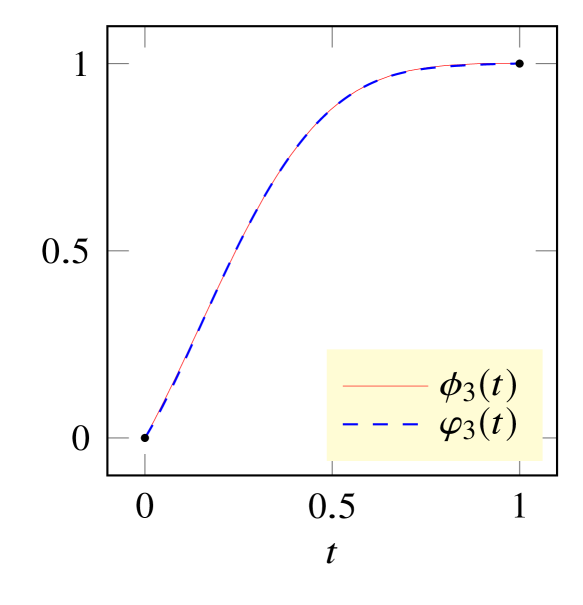
(a) The plots of the functions $\phi_{3}$ and $\varphi_{3}$.

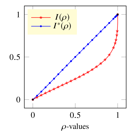
(b) The plots of $I$ and $I^{*}$ in $\mathcal{N}_{3}\mathopen{}\mathclose{{}\left(\mathbf{0},{\mathrel{\mathchoice{\ooalign{$\displaystyle\mathbf{\Sigma}$\cr\hfil$\displaystyle|$\hfil\cr}}{\ooalign{$\textstyle\mathbf{\Sigma}$\cr\hfil$\textstyle|$\hfil\cr}}{\ooalign{$\scriptstyle\mathbf{\Sigma}$\cr\hfil$\scriptstyle|$\hfil\cr}}{\ooalign{$\scriptscriptstyle\mathbf{\Sigma}$\cr\hfil$\scriptscriptstyle|$\hfil\cr}}}}_{3}(\rho)}\right)$ case.

Figure 4.1: The functions $\phi_{3}$ and $\varphi_{3}$, as well as the indices $I$ and $I^{*}$ in $\mathcal{N}_{3}\mathopen{}\mathclose{{}\left(\mathbf{0},{\mathrel{\mathchoice{\ooalign{$\displaystyle\mathbf{\Sigma}$\cr\hfil$\displaystyle|$\hfil\cr}}{\ooalign{$\textstyle\mathbf{\Sigma}$\cr\hfil$\textstyle|$\hfil\cr}}{\ooalign{$\scriptstyle\mathbf{\Sigma}$\cr\hfil$\scriptstyle|$\hfil\cr}}{\ooalign{$\scriptscriptstyle\mathbf{\Sigma}$\cr\hfil$\scriptscriptstyle|$\hfil\cr}}}}_{3}(\rho)}\right)$ case.

Both $\varphi_{2}\colon[0,1]\to[0,1]$ and $\varphi_{3}\colon[0,1]\to[0,1]$ are strictly increasing functions. The Lagrange interpolation polynomial formula, that has been used for the cases of dimension 2 and 3, often leads to find interpolating polynomials that are not strictly monotone; hence, it is wise to avoided for dimensions greater than 3. For any specific value of $d$, we propose the use the MonoPoly R package (Turlach and Murray, 2019) to find an appropriate, strictly monotone, polynomial for approximating the standardized index. The procedure is presented by Algorithm 4.1; in Section V of the Supplementary Material, we provide a realization of Step 2 of the algorithm.

Algorithm 4.1 Computation of the approximate standardized index $I^{*}$.

1: Let $0\leq\rho\leq 1$ and consider $\boldsymbol{X}_{\rho}\sim\mathcal{N}_{d}(\mathbf{0},{\mathrel{\mathchoice{\ooalign{$\displaystyle\mathbf{\Sigma}$\cr\hfil$\displaystyle|$\hfil\cr}}{\ooalign{$\textstyle\mathbf{\Sigma}$\cr\hfil$\textstyle|$\hfil\cr}}{\ooalign{$\scriptstyle\mathbf{\Sigma}$\cr\hfil$\scriptstyle|$\hfil\cr}}{\ooalign{$\scriptscriptstyle\mathbf{\Sigma}$\cr\hfil$\scriptscriptstyle|$\hfil\cr}}}}_{d}(\rho))$ as in Remark 2.1, and consider the vector of $\rho$-values $\boldsymbol{\varrho}=(0,0.4,0.8,0.95,0.99,1)$. Then compute $\boldsymbol{I}\equiv\boldsymbol{I}(\boldsymbol{\varrho})\doteq(I(\varrho_{1}),\ldots,(\varrho_{6}))$. $\triangleright$ By definition, $I(0)=0$ and $I(1)=1$.

2: Fit a monotone polynomial on $[0,1]$ of degree $7$, say $\varphi_{d}$, to the data set $\{(I(\varrho_{j}),\varrho_{j}),\ j=1,\ldots,6\}$.

3: Define $I^{*}\doteq\varphi_{d}(I)$.

Based on the values of $I^{*}$ we define four levels of dependence.

Definition 4.1.

Let $\boldsymbol{X}\in\mathcal{X}^{d}$. We say that $\boldsymbol{X}$ has a weak, mild, strong or very strong dependence structure if $I^{*}$ belongs to $[0,0.25)$, $[0.25,0.5)$, $[0.5,0.75)$ or $[0.75,1]$ respectively.

Remark 4.1.

Via numerical study, we observe that when the underlying distribution is $\mathcal{N}_{2}\mathopen{}\mathclose{{}\left(\mathbf{0},{\mathrel{\mathchoice{\ooalign{$\displaystyle\mathbf{\Sigma}$\cr\hfil$\displaystyle|$\hfil\cr}}{\ooalign{$\textstyle\mathbf{\Sigma}$\cr\hfil$\textstyle|$\hfil\cr}}{\ooalign{$\scriptstyle\mathbf{\Sigma}$\cr\hfil$\scriptstyle|$\hfil\cr}}{\ooalign{$\scriptscriptstyle\mathbf{\Sigma}$\cr\hfil$\scriptscriptstyle|$\hfil\cr}}}}_{2}(\rho)}\right)$ (see Vexler et al., 2019) or $\mathcal{N}_{3}\mathopen{}\mathclose{{}\left(\mathbf{0},{\mathrel{\mathchoice{\ooalign{$\displaystyle\mathbf{\Sigma}$\cr\hfil$\displaystyle|$\hfil\cr}}{\ooalign{$\textstyle\mathbf{\Sigma}$\cr\hfil$\textstyle|$\hfil\cr}}{\ooalign{$\scriptstyle\mathbf{\Sigma}$\cr\hfil$\scriptstyle|$\hfil\cr}}{\ooalign{$\scriptscriptstyle\mathbf{\Sigma}$\cr\hfil$\scriptscriptstyle|$\hfil\cr}}}}_{3}(\rho)}\right)$ (see Table III.1, Section III of the Supplementary Material) the index $I$ is an increasing function of $\rho\in[0,1]$. We conjecture that this is true whenever the underlying distribution is $\mathcal{N}_{d}\mathopen{}\mathclose{{}\left(\mathbf{0},{\mathrel{\mathchoice{\ooalign{$\displaystyle\mathbf{\Sigma}$\cr\hfil$\displaystyle|$\hfil\cr}}{\ooalign{$\textstyle\mathbf{\Sigma}$\cr\hfil$\textstyle|$\hfil\cr}}{\ooalign{$\scriptstyle\mathbf{\Sigma}$\cr\hfil$\scriptstyle|$\hfil\cr}}{\ooalign{$\scriptscriptstyle\mathbf{\Sigma}$\cr\hfil$\scriptscriptstyle|$\hfil\cr}}}}_{d}(\rho)}\right)$ for any value of $d$.

5.   Investigation of the index in view of the dependence axioms

Here we investigate the classes of random vectors in which Axioms $A_{1}$ to $A_{8}$ and $A^{\prime}_{1}$ to $A^{\prime}_{4}$ hold; notice that Axiom $A_{7}$ is only mentioned in the case $d=2$.

For Axioms $A_{4}$ and $A^{\prime}_{1}$ we define the class of random vectors $\mathcal{X}^{d}_{1}$, while for Axioms $A_{3}$, $A_{5}$ and $A^{\prime}_{3}$ we define the class $\mathcal{X}^{d}_{2}$. We first state the conditions that determine these classes of random vectors.

1. One can detect at least a subscript $j=1,\ldots,2^{d}$ for which the Kendall function of $\boldsymbol{X}_{j}\in\mathcal{R}(\boldsymbol{X})$ is such that $K_{j}(t)-K_{\varPi}(t)\geq 0$ or $\leq 0$ for all $0\leq t\leq 1$. That is, we can find at least one Kendall plot that does not cross the diagonal line.

2. One can detect at least two subscripts $j=1,\ldots,2^{d}$ for which the functions of $\boldsymbol{X}_{j}\in\mathcal{R}(\boldsymbol{X})$ are such that $K_{j}(t)-K_{\varPi}(t)\leq 0$ for all $0\leq t\leq 1$. That is, we can find at least two Kendall plots that lie below the diagonal line.

Consider now the following subclasses of $\mathcal{X}^{d}_{0}$:

$$\mathcal{X}^{d}_{1}\doteq\{\boldsymbol{X}\in\mathcal{X}^{d}_{0}\colon\textrm{\ref{C1} holds}\};\quad\mathcal{X}^{d}_{2}\doteq\{\boldsymbol{X}\in\mathcal{X}^{d}_{0}\colon\textrm{\ref{C2} holds}\}.$$

Note that $\mathcal{X}^{d}_{2}\subset\mathcal{X}^{d}_{1}\subset\mathcal{X}^{d}_{0}$. Moreover, $\mathcal{X}^{d}_{2}$ is not an empty set; for each continuous rv $X$, the random vector $(X,\ldots,X)^{T}$ on $\mathds{R}^{d}$ belongs to $\mathcal{X}^{d}_{2}$ because its Kendall function is $K(t)=t$, $0\leq t\leq 1$, see the proof of Equation (4.2) in Appendix D, which lies below of $K_{\varPi}(t)$, $0\leq t\leq 1$ (set $g(t)=K_{\varPi}(t)-t$, $0\leq t\leq 1$, and observe that $g$ is a concave function with $g(0)=g(1)=0$). In Section 6 we present Algorithm 6.1, that one can use to check whether the data come from a distribution that belongs in $\mathcal{X}^{d}_{1}$ or $\mathcal{X}^{d}_{2}$.

We are now in a position to investigate Axioms $A_{1}$ to $A_{8}$ as well as $A^{\prime}_{1}$ to $A^{\prime}_{4}$.

Proposition 5.1.

For the index of dependence $I$ defined by (4.3) we have: (a) Axioms $A_{1}$, $A_{2}$, $A_{6}$, $A_{7}$ and $A_{8}$ hold in $\mathcal{X}^{d}_{0}$; (b) Axiom $A_{4}$ holds in $\mathcal{X}^{d}_{1}$; (c) Axioms $A_{3}$ and $A_{5}$ hold in $\mathcal{X}^{d}_{2}$. .

Proposition 5.2.

For the index of dependence $I$ defined by (4.3) we have: (a) Axiom $A^{\prime}_{1}$ holds in $\mathcal{X}^{d}_{1}$; (b) Axioms $A^{\prime}_{2}$ and $A^{\prime}_{4}$ hold in $\mathcal{X}^{d}_{0}$; (c) Axioms $A^{\prime}_{3}$ holds in $\mathcal{X}^{d}_{2}$. .

Remark 5.1.

1. Propositions 5.1 and 5.2 say that $I$ is a measure of dependence for the structure of random vectors in $\mathcal{X}^{d}_{2}$, in both Rényi’s as well as Móri and Székely’s definitions.

2. The standardized index $I^{*}=\varphi_{d}(I)$ is also a measure of dependence for the structure of random vectors in $\mathcal{X}^{d}_{2}$, in both Rényi’s as well as Móri and Székely’s definitions, whenever $\varphi_{d}$ is a bijective increasing mapping.

3. $I$ and $I^{*}$ are indices of the dependence structure for random vectors in $\mathcal{X}^{d}_{0}$.

4. Consider a random vector $\boldsymbol{X}\sim F$ in $\mathcal{X}^{d}_{0}$, and suppose its marginal cdfs are $F_{i}(t)=\operatorname{\mathds{P}}(X_{i}\leq t)$, $i=1,\ldots,d$. Applying the probability integral transform to each $X_{i}$, the random vector $\boldsymbol{U}=(U_{1},\ldots,U_{d})^{T}\doteq(F_{1}(X_{1}),\ldots,F_{d}(X_{d}))^{T}$ has marginals that are uniformly distributed on $[0,1]$. The copula of $\boldsymbol{X}$ is defined as the cdf of $\boldsymbol{U}$, $C(\boldsymbol{u})=\operatorname{\mathds{P}}(\boldsymbol{U}\leq\boldsymbol{u})$; notice that the copula $C$ contains all information on the dependence structure between the components of $\boldsymbol{X}$. Since Axiom $A_{6}$ holds, see Proposition 5.1a, we have that the index $I$, and hence $I^{*}$, is a copula-based index of dependence; namely, $I_{F}=I_{C}$ and $I^{*}_{F}=I^{*}_{C}$.

6.   Estimating $\mathbf{AUK}$, $\boldsymbol{I}$, $\boldsymbol{I^{*}}$

Suppose that a random sample $\boldsymbol{X}_{i}$, $i=1,\ldots,n$, has been drawn from a $d$-dimensional distribution $F$. For each $\boldsymbol{s}_{j}\in\mathds{S}^{d}$, $j=1,\ldots,d$, set $\boldsymbol{X}_{ij}=\operatorname{diag}(\boldsymbol{s}_{j})\boldsymbol{X}_{i}$, $i=1,\ldots,n$, which is a random sample from $\boldsymbol{X}_{j}=\operatorname{diag}(\boldsymbol{s}_{j})\boldsymbol{X}$; and let $\mathbb{F}_{nj}$ denote the empirical cumulative distribution function (ecdf) of $\boldsymbol{X}_{ij}=\operatorname{diag}(\boldsymbol{s}_{j})\boldsymbol{X}_{i}$, $i=1,\ldots,n$,

$$\mathbb{F}_{nj}(\boldsymbol{x})=\frac{1}{n}\sum_{i=1}^{n}\mathds{1}_{\{\boldsymbol{X}_{ij}\leq\boldsymbol{x}\}},\quad\boldsymbol{x}\in\mathds{R}^{d};$$

consider the corresponding empirical Kendall distribution function

$$\mathbb{K}_{nj}(t)=\frac{1}{n}\sum_{i=1}^{n}\mathds{1}_{\{\mathbb{F}_{nj}(\boldsymbol{X}_{ij})\leq t\}},\quad t\in[0,1].$$ (6.1)

Let $\hat{T}_{nj}\sim\mathbb{K}_{nj}$, $j=1,\ldots,d$. By virtue of the formula $\mathrm{AUK}=\operatorname{\mathds{E}}\mathopen{}\mathclose{{}\left\{1-K_{\varPi}(T)}\right\}$, we can estimate the $\mathrm{AUK}_{j}$s in a nonparametric manner via the statistic

$$\hat{\mathrm{AUK}}_{nj}=\operatorname{\mathds{E}}\mathopen{}\mathclose{{}\left\{1-K_{\varPi}(\hat{T}_{nj})}\right\}=1-\frac{1}{n}\sum_{i=1}^{n}K_{\varPi}(\hat{T}_{nij}),$$

where $\hat{T}_{nij}=\mathbb{F}_{nj}(\boldsymbol{X}_{ij})$, $i=1,\ldots,n$. Then, we get nonparametric estimations of $I$ and $I^{*}$, $\hat{I}_{n}$ and $\hat{I}^{*}_{n}$ respectively, by

$$\hat{I}_{n}\doteq\mathopen{}\mathclose{{}\left(2^{d-2}-2^{1-d}+2^{1-2d}}\right)^{-1/2}\|\hat{\boldsymbol{D}}_{n}-\boldsymbol{\varDelta}\|\quad\textrm{and}\quad\hat{I}^{*}_{n}\doteq\varphi_{d}(\hat{I}_{n}),$$

where $\hat{\boldsymbol{D}}_{n}=(\hat{\mathrm{AUK}}_{n1},\ldots,\hat{\mathrm{AUK}}_{n2^{d}})^{T}$.

We are interested in studying the consistency of the proposed estimators. Theorem C.3 presents the consistency of $\mathbb{K}_{nj}$s, see in Appendix. Based on this result, in Appendix D, we prove that $\hat{\mathrm{AUK}}_{nj}$ is a strongly consistent estimator of $\mathrm{AUK}_{j}$, that is,

$$\hat{\mathrm{AUK}}_{nj}\xlongrightarrow{\textrm{\begin{picture}(0.0,0.0)\put(0.0,0.0){\makebox(-1.75,-0.5)[]{$\mathrm{as}$}}\end{picture}}}\mathrm{AUK}_{j}\textrm{ for all }j=1,\ldots,2^{d};$$ (6.2)

hence, using the continuous mapping theorem, $\hat{I}_{n}\xlongrightarrow{\textrm{\begin{picture}(0.0,0.0)\put(0.0,0.0){\makebox(-1.75,-0.5)[]{$\mathrm{as}$}}\end{picture}}}I$ as well as $\hat{I}^{*}_{n}\xlongrightarrow{\textrm{\begin{picture}(0.0,0.0)\put(0.0,0.0){\makebox(-1.75,-0.5)[]{$\mathrm{as}$}}\end{picture}}}I^{*}$, that is, both $\hat{I}_{n}$ and $\hat{I}^{*}_{n}$ are strongly consistent estimators of $I$ and $I^{*}$ respectively.

In addition to the consistency of $\hat{I}_{n}$ and $\hat{I}^{*}_{n}$, Theorem C.3 gives a graphical method for checking if the underlying data distribution belongs in $\mathcal{X}^{d}_{1}$ or $\mathcal{X}^{d}_{2}$; Algorithm 6.1 enables one to carry out such a check.

Algorithm 6.1 Algorithm for checking if the underlying data distribution belongs in $\mathcal{X}^{d}_{1}$ or $\mathcal{X}^{d}_{2}$.

1: Compute $K_{\varPi}$ and $K_{nj}$, $j=1,\dots,2^{d}$, using the formulas (4.1) and (6.1).

2: Visualize the curves $(K_{nj}(t),K_{\varPi}(t))$, $0\leq t\leq 1$, for all $j=1,\dots,2^{d}$.

3: Decision Rule:

1. If there is at least one curve that does not cross the diagonal line, then the data set is from $\mathcal{X}^{d}_{1}$.

2. If there are at least two curves that lie below the diagonal line, then the data set is from $\mathcal{X}^{d}_{2}$.

7.   Testing joint or mutual dependence

In this section, we investigate the null hypothesis of total independence. Let $\hat{\mathrm{AUK}}_{n}$ be the estimator of $\mathrm{AUK}$ of the original/non-rotated data distribution; namely, the $\hat{\mathrm{AUK}}_{nj}$ that corresponds to $\boldsymbol{s}_{j}=(+,\ldots,+)^{T}\in\mathds{S}^{d}$.

We are interested in testing the hypothesis

$$H_{0}\colon F(\boldsymbol{x})=F_{1}(x_{1})\cdots F_{d}(x_{d})\quad\textrm{versus}\quad H_{1}\colon F(\boldsymbol{x})\neq F_{1}(x_{1})\cdots F_{d}(x_{d}).$$

For testing this hypothesis, we propose the statistic

$$z_{n}=\surd{n}(\hat{\mathrm{AUK}}_{n}-1/2)/\sigma_{\varPi},$$

where the true value of the standard deviation $\sigma_{\varPi}$ can be computed explicitly through the relations (7.1b), (7.2a)–(7.2c) given below. In the case $d=2$, we have computed $\sigma_{\varPi}=(19/432)^{1/2}$ — see Appendix B.

We now prove the asymptotic normality of the $\hat{\mathrm{AUK}}_{n}$ under this null hypothesis. The result is derived through the asymptotic behavior of a modified Kendall process that originally was defined by Genest and Rivest (1993) as well as the results given by Barbe et al. (1996). For easy reference, we state these results in Appendix B. In Appendix B, we prove that

$$\surd{n}(\hat{\mathrm{AUK}}_{n}-1/2)\stackrel{{\scriptstyle H_{0}}}{{\rightsquigarrow}}\mathcal{N}(0,\sigma_{\varPi}^{2}),\quad\textrm{with}$$ (7.1a)

$$\sigma_{\varPi}^{2}=\int_{0}^{1}\int_{0}^{1}k_{\varPi}(s)\varGamma_{\varPi}(s,t)k_{\varPi}(t)\operatorname{d\textrm{$s$}}\operatorname{d\textrm{$t$}}=2\iint_{0<s<t<1}k_{\varPi}(s)\varGamma_{\varPi}(s,t)k_{\varPi}(t)\operatorname{d\textrm{$s$}}{\operatorname{d\textrm{$t$}}},$$ (7.1b)

where

$$\varGamma_{\varPi}(s,t)=K_{\varPi}(s\wedge t)-K_{\varPi}(s)K_{\varPi}(t)+k_{\varPi}(s)k_{\varPi}(t)R_{\varPi}(s,t)-k_{\varPi}(t)Q_{\varPi}(s,t)-k_{\varPi}(s)Q_{\varPi}(t,s),$$ (7.2a)

where $$\boldsymbol{u}\wedge\boldsymbol{v} \boldsymbol{u} \boldsymbol{v}$$ denotes the componentwise minimum between and ,

$$Q_{\varPi}(s,t)=(s\wedge t)\sum_{i=1}^{d}\frac{\ln^{i}(t/s\wedge t)}{i!}-tK_{\varPi}(s)$$ (7.2b)

$$R_{\varPi}(s,t)=\operatorname{\mathds{E}}\mathopen{}\mathclose{{}\left(\exp\mathopen{}\mathclose{{}\left[\sum_{i=1}^{d}\min\mathopen{}\mathclose{{}\left\{\ln(s)U_{1}^{(i)},\ln(t)U_{2}^{(i)}}\right\}}\right]}\right)-st,$$ (7.2c)

where $$\boldsymbol{U}_{j}=\mathopen{}\mathclose{{}\left(U_{j}^{(1)},\ldots,U_{j}^{(d)}}\right)^{T} j=1,2 [0,1]^{d}$$, , are independent random vectors uniformly distributed on the simplex in .

Therefore, at significance level $\alpha$, the asymptotic rejection region is $R=\{|z_{n}|>z_{\alpha/2}\}$, where $z_{\alpha}$ is the upper $\alpha$-point of the standard normal distribution. Hereafter, we call this test as $\mathrm{AUK}$ test for total independence or simply $\mathrm{AUK}$ independence test.

We investigate further the proposed independence test in the bivariate case. The distribution of $z_{n}$ is asymptotically $\mathcal{N}(0,1)$. Table 7.1 contains the 90th, 95th and 99th percentiles of the empirical distribution of $|z_{n}|$ generated by simulation of $10^{5}$ samples of various sizes $n$ from the standard bivariate uniform distribution. For a sample of size $n$, the proposed $\alpha$-level independence test is

$$\textrm{reject the total independence if }|z_{n}|>p_{d=2,n;1-\alpha},$$

where $p_{d=2,n;1-\alpha}$ is given in Table 7.1 noting that $p_{d=2,\infty;1-\alpha}=z_{\alpha/2}$.

Table 7.1: Empirical percentiles of the distribution of $|z_{n}|$ for random samples of size $n$ drawn standard bivariate uniform distribution.

$n$	30	$50$	$70$	$100$	$150$	$200$	$300$	$400$	$500$	$750$	$1000$	$\infty$
$p_{d=2,n;0.90}$	2.30	2.11	2.01	1.93	1.84	1.79	1.74	1.72	1.71	1.68	1.67	1.65
$p_{d=2,n;0.95}$	2.62	2.44	2.34	2.25	2.17	2.12	2.06	2.05	2.03	2.01	1.98	1.96
$p_{d=2,n;0.99}$	3.19	3.05	2.95	2.87	2.78	2.75	2.68	2.67	2.65	2.63	2.60	2.57

Suppose we have a $d$-dimensional continuous cdf $G$ such that the corresponding $\mathrm{AUK}\neq 1/2$. Due to consistency, see (6.2), and using the continuous mapping theorem, we have that $|\hat{\mathrm{AUK}}_{n}-1/2|\xlongrightarrow{\textrm{\begin{picture}(0.0,0.0)\put(0.0,0.0){\makebox(-1.75,-0.5)[]{$\mathrm{as}$}}\end{picture}}}|\mathrm{AUK}-1/2|\neq 0$; therefore, the statistic $|z_{n}|$ diverges almost surely to infinity; thus, if the alternative hypothesis is $F=G$, the power of the test goes to 1. Consequently, the proposed $\hat{\mathrm{AUK}}_{n}$-based test for total independence is consistent against the set of alternatives of $d$-dimensional continuous cdfs with $\mathrm{AUK}\neq 1/2$.

We now offer an alternative way to compute the standard deviation $\sigma_{\varPi}$. Recall that the true standard deviation $\sigma_{\varPi}$ can be computed exactly through the relations (7.1b) and (7.2a)–(7.2c). Since $\boldsymbol{U}_{j}$s are uniformly distributed on the $d$-dimensional probability simplex, it is rather laborious to compute the exact value of the true standard deviation $\sigma_{\varPi}$ for general values of $d$; the difficulty is due to the calculations on the simplex. Thus, we provide a Monte Carlo based algorithm for estimating the standard deviation $\sigma_{\varPi}$.

Algorithm 7.1 Approximation of the standard deviation $\sigma_{\varPi}$.

1: Let $d$ be the dimension of interest. Consider a $d$-dimensional continuous distribution with independent components; without loss of generality, consider the standard $d$-dimensional uniform distribution, say $\boldsymbol{U}$, that is the distribution with density $f_{\boldsymbol{U}}(\boldsymbol{u})=u_{1}\cdots u_{d}$, $\boldsymbol{u}=(u_{1},\dots,u_{d})^{T}\in[0,1]^{d}$.

2: Let $n$ and $r$ be two large positive integer numbers. Generate $r$ independent random samples of size $n$ from $F_{\boldsymbol{U}}$, say $\boldsymbol{U}_{i,j}$, $i=1,\dots,n$ and $j=1,\dots,r$.

3: Based on the $j$th random sample, $\boldsymbol{U}_{i,j}$, $i=1,\dots,n$, compute the $\hat{\mathrm{AUK}}_{j}$ and then $A_{i}\doteq\surd{n}(\hat{\mathrm{AUK}}_{j}-1/2)$, $j=1,\dots,r$.

4: Define $\hat{\sigma}_{\varPi}$ to be the sample standard deviation of $A_{1},\dots,A_{r}$.

Using Algorithm 7.1 with $r=10000$ and $n=50000$, we offer estimations $\hat{\sigma}_{\varPi}$ for the cases $d=2,\dots,10$. Observe that in the case $d=2$ the estimated value $\hat{\sigma}_{\varPi}=0.20988$ is very closed to the true value $\sigma_{\varPi}=(19/432)^{1/2}\approxeq 0.20972$ ($\hat{\sigma}_{\varPi}/\sigma_{\varPi}=1.000779$).

Table 7.2: Mode Carlo estimate of $\sigma_{\varPi}$, using Algorithm 7.1 with $r=10000$ and $n=50000$, when $d=2,\dots,10$.

$d$	2	3	4	5	6	7	8	9	10
$\hat{\sigma}_{\varPi}$	0.20988	0.19383	0.16254	0.12511	0.09407	0.06853	0.04912	0.03395	0.02377

To make our test practical for small sample sizes $n$, we present an algorithm to approximate the percentiles of the distribution of $|z_{n}|$. Suppose $\boldsymbol{X}_{1},\ldots,\boldsymbol{X}_{n}$ is a random sample of size $n$ from a $d$-dimensional continuous distribution $F$ and we are interested in testing the null hypothesis of total independence. We use the statistic $z_{n}$; and the rejection region of the null hypothesis at $\alpha$-significant level is $|z_{n}|>p_{d,n;1-\alpha}$, where $p_{d,n;1-\alpha}$ denote the $(1-\alpha)$-percentile point of the distribution of $|z_{n}|$. If the sample size $n$ is large, that is $n>\max\{1000,100d\}$, then $p_{d,n;1-\alpha}=p_{d,\infty;1-\alpha}=z_{\alpha/2}$ else we approximate this percentile point using Algorithm 7.2.

Algorithm 7.2 Approximation of the percentiles of the distribution of $|z_{n}|$ for small sample sizes.

1: Consider the standard $d$-dimensional uniform distribution, say $\boldsymbol{U}$, that is the distribution with density $f_{\boldsymbol{U}}(\boldsymbol{u})=u_{1}\cdots u_{d}$, $\boldsymbol{u}=(u_{1},\dots,u_{d})^{T}\in[0,1]^{d}$.

2: For a large positive integer $r$, generate $r$ independent random samples of size $n$ from $F_{\boldsymbol{U}}$, say $\boldsymbol{U}_{i,j}$, $i=1,\dots,n$ and $j=1,\dots,r$.

3: Based on the $j$th random sample, $\boldsymbol{U}_{i,j}$, $i=1,\dots,n$, compute the corresponding $|z_{n}|$-value, say $|z_{n;j}|$, $j=1,\dots,r$.

4: Define $p_{d,n;1-\alpha}$ to be the $(1-\alpha)$-percentile point of the distribution of the values $|z_{n;1}|,\dots,|z_{n;r}|$.

Notice that if the dimension $d$ is small, for example $d\leq 10$, and since $n\leq 1000$, the number of Monte Carlo repetitions $r=10^{4}$ is sufficient for an accurate approximation of $p_{d,n;1-\alpha}$ using Algorithm 7.2 with low computational cost.

Remark 7.1.

For the estimation of $\mathrm{AUK}$ we used the relationship $\mathrm{AUK}=\operatorname{\mathds{E}}\mathopen{}\mathclose{{}\left\{1-K_{\varPi}(T)}\right\}$. The study of the asymptotic behavior of this estimator, i.e. the estimator $\hat{\mathrm{AUK}}_{n}$ that is presented in Section 7, as well as its limit distribution under the hypothesis of total independence go through the Kendall process and the functional delta-method. Another way for estimating the $\mathrm{AUK}$ is via use of the formula $\mathrm{AUK}=\operatorname{\mathds{P}}(T\leq\varPi)$; then, similar to Pfister et al. (2018), a kernel-based estimation of $\mathrm{AUK}$ seems to be feasible and then the use of $U$- or $V$-statistics theory allows one to obtain the asymptotic distribution of the statistic.

We now discuss the possibility of a general $\mathrm{AUK}$-based hypothesis test, i.e. $H_{0}\colon\mathrm{AUK}=a_{0}$ versus $H_{1}\colon\mathrm{AUK}\neq a_{0}$ for a fixed constant $a_{0}\in[2^{-d},1]$; until now we have only studied the case $a_{0}=1/2$. We first present the following example.

Example 7.1.

Let $\boldsymbol{X}=(X_{1},X_{2})^{T}$ be a bivariate rv uniformly distributed on the circumference of the circle centered at the origin with a radius of 1. The ordinary Kendall cdf of $\boldsymbol{X}$ is $K_{\boldsymbol{X}}(t)=\mathds{1}_{\{0\leq t<1/2\}}(t+1/4)+\mathds{1}_{\{1/2\leq t\leq 1\}}$ (see Vexler et al., 2019, p. 426) and so $\mathrm{AUK}_{\boldsymbol{X}}=11/16-\ln(2)/4$. Consider now the bivariate normal rv $\boldsymbol{Z}=(Z_{1},Z_{2})^{T}\sim\mathcal{N}_{2}\mathopen{}\mathclose{{}\left(\mathbf{0},\mathopen{}\mathclose{{}\left({1\atop-0.073622}~{}{-0.073622\atop 1}}\right)}\right)$. A numerical computation gives $\mathrm{AUK}_{\boldsymbol{Z}}=\mathrm{AUK}_{\boldsymbol{X}}$. One can verify that hypotheses $\mathrm{H}_{1}$ and $\mathrm{H}_{2}$, see Appendix B, hold and so Theorem B.1 also holds for the random vector $\boldsymbol{Z}$. On the other hand, hypothesis $\mathrm{H}_{1}$ does not hold for the random vector $\boldsymbol{X}$; hence, the statement of Theorem B.1 is not true for this case.

In view of the above example, we conclude that it is not possible to construct general $\mathrm{AUK}$-based hypotheses tests, as these are described at the beginning of the paragraph.

8.   Simulation study

In this section, we present a simulation study designed with two specific goals in mind. First, we are interested in understanding the behavior of the proposed indices of dependence as a function of the sample size, the type and the degree of dependence that a data set exhibits.

Our second goal relates to the evaluation of the performance of the proposed tests of independence, in terms of level of significance and power of the tests. In what follows, we present evidence of this performance by simulating data from a range of distributions and hence, dependence structures.

8.1.   The estimators $\hat{I}_{n}$ and $\hat{I}^{*}_{n}$

We first present a simulation study for the proposed empirical dependence indices.

8.1.1.   Normal case

We simulate $r=1000$ random samples of size $n=100,200,500,1000$ from the trivariate normal $\mathcal{N}_{3}(\mathbf{0},{\mathrel{\mathchoice{\ooalign{$\displaystyle\mathbf{\Sigma}$\cr\hfil$\displaystyle|$\hfil\cr}}{\ooalign{$\textstyle\mathbf{\Sigma}$\cr\hfil$\textstyle|$\hfil\cr}}{\ooalign{$\scriptstyle\mathbf{\Sigma}$\cr\hfil$\scriptstyle|$\hfil\cr}}{\ooalign{$\scriptscriptstyle\mathbf{\Sigma}$\cr\hfil$\scriptscriptstyle|$\hfil\cr}}}}_{3}(\boldsymbol{\rho}))$ distribution (for the variance/covariance matrix ${\mathrel{\mathchoice{\ooalign{$\displaystyle\mathbf{\Sigma}$\cr\hfil$\displaystyle|$\hfil\cr}}{\ooalign{$\textstyle\mathbf{\Sigma}$\cr\hfil$\textstyle|$\hfil\cr}}{\ooalign{$\scriptstyle\mathbf{\Sigma}$\cr\hfil$\scriptstyle|$\hfil\cr}}{\ooalign{$\scriptscriptstyle\mathbf{\Sigma}$\cr\hfil$\scriptscriptstyle|$\hfil\cr}}}}_{3}(\boldsymbol{\rho})$ see (2.2a)), for various values of $n$ and $\boldsymbol{\rho}=(\rho_{12},\rho_{13},\rho_{23})$. Based on these samples we compute the averages (and the Monte Carlo mean square error) of $\hat{I}$ and $\hat{I}^{*}$; Table 8.1 presents the results. In all cases the empirical mean square error of the indices tends to zero as $n$ goes to infinity, confirming the consistency of the estimation for both $\hat{I}$ and $\hat{I}^{*}$ estimators. Figure 8.1 presents illustrations of graphs of a single sample $\{\boldsymbol{X}_{1},\ldots,\boldsymbol{X}_{n}\}$ of size $n=1000$ drawn from these distributions. The standardized index $I^{*}$ indicates that, see Definition 4.1, the normal distributions with $(\rho_{12},\rho_{13},\rho_{23})\in\{(0,0,0),(-0.1,-0.1,0.2)\}$ have a weak dependence level, that the ones with $(\rho_{12},\rho_{13},\rho_{23})\in\{(-0.3,-0.3,-0.3),(0.2,0.3,0.4)\}$ have a mild dependence level, while the distributions with $(\rho_{12},\rho_{13},\rho_{23})\in\{(0.7,0.5,0),(0.2,-0.8,0)\}$ have a strong dependence level, and that normal distributions with $(\rho_{12},\rho_{13},\rho_{23})\in\{(1,1,1),(-0.5,-0.5,-0.5),(0.1,0.2,-0.9)\}$ have a very strong dependence level. On the other hand, the case $(\rho_{12},\rho_{13},\rho_{23})=(-0.5,-0.5,0.5)$ lies in the frontier between mild and strong dependence level.

Table 8.1: Monte Carlo averages (and associated mean square error) of $I$ and $I^{*}$; the number of Monte Carlo repetitions is $r=1000$. Random samples of size $n$ are drawn from different $\mathcal{N}_{3}\mathopen{}\mathclose{{}\left(\mathbf{0},{\mathrel{\mathchoice{\ooalign{$\displaystyle\mathbf{\Sigma}$\cr\hfil$\displaystyle|$\hfil\cr}}{\ooalign{$\textstyle\mathbf{\Sigma}$\cr\hfil$\textstyle|$\hfil\cr}}{\ooalign{$\scriptstyle\mathbf{\Sigma}$\cr\hfil$\scriptstyle|$\hfil\cr}}{\ooalign{$\scriptscriptstyle\mathbf{\Sigma}$\cr\hfil$\scriptscriptstyle|$\hfil\cr}}}}_{3}(\boldsymbol{\rho})}\right)$ distributions, for various values of $n$ and $\boldsymbol{\rho}=(\rho_{12},\rho_{13},\rho_{23})$.

(a) $(\rho_{12},\rho_{13},\rho_{23})=(0,0,0)$; true values of indices: $I=0$ and $I^{*}=0$.

	$n$
	100	$200$	$500$	$1000$
$\hat{I}_{n}$	.097(.009)	.059(.004)	.032(.001)	.022(.000)
$\hat{I}^{*}_{n}$	.186(.035)	.109(.012)	.057(.003)	.037(.001)

(b) $(\rho_{12},\rho_{13},\rho_{23})=(1,1,1)$; true values of indices: $I=1$ and $I^{*}=1$.

	$n$
	100	$200$	$500$	$1000$
$\hat{I}_{n}$	.739(.068)	.833(.028)	.912(.008)	.947(.003)
$\hat{I}^{*}_{n}$	.985(.000)	.994(.000)	.998(.000)	.999(.000)

(c) $(\rho_{12},\rho_{13},\rho_{23})=(-0.5,-0.5,0.5)$; true values of indices: $I=0.243$ and $I^{*}=0.5$.

	$n$
	100	$200$	$500$	$1000$
$\hat{I}_{n}$	.222(.001)	.229(.000)	.236(.000)	.239(.000)
$\hat{I}^{*}_{n}$	.459(.004)	.472(.002)	.487(.001)	.493(.000)

(d) $(\rho_{12},\rho_{13},\rho_{23})=(-0.5,-0.5,-0.5)$; true values of indices: $I=0.554$ and $I^{*}=0.92$.

	$n$
	100	$200$	$500$	$1000$
$\hat{I}_{n}$	.418(.019)	.464(.008)	0.505(.002)	0.525(.001)
$\hat{I}^{*}_{n}$	.794(.016)	.846(.006)	0.885(.001)	0.900(.000)

(e) $(\rho_{12},\rho_{13},\rho_{23})=(0.10,0.20,-0.90)$; true values of indices: $I=0.461$ and $I^{*}=0.842$.

	$n$
	100	$200$	$500$	$1000$
$\hat{I}_{n}$	.382(.006)	.413(.002)	.438(.000)	.449(.000)
$\hat{I}^{*}_{n}$	.745(.010)	.787(.003)	.818(.000)	.829(.000)

(f) $(\rho_{12},\rho_{13},\rho_{23})=(0.70,0.50,0)$; true values of indices: $I=0.363$ and $I^{*}=0.717$.

	$n$
	100	$200$	$500$	$1000$
$\hat{I}_{n}$	.311(.003)	.330(.001)	.348(.000)	.355(.000)
$\hat{I}^{*}_{n}$	.631(.008)	.664(.003)	.693(.001)	.704(.000)

(g) $(\rho_{12},\rho_{13},\rho_{23})=(0.20,-0.80,0)$; true values of indices: $I=0.334$ and $I^{*}=0.671$.

	$n$
	100	$200$	$500$	$1000$
$\hat{I}_{n}$	.291(.002)	.307(.001)	.322(.000)	.327(.000)
$\hat{I}^{*}_{n}$	.594(.007)	.624(.003)	.651(.001)	.659(.000)

(h) $(\rho_{12},\rho_{13},\rho_{23})=(-0.30,-0.30,-0.30)$; true values of indices: $I=0.204$ and $I^{*}=0.420$.

	$n$
	100	$200$	$500$	$1000$
$\hat{I}_{n}$	.192(.001)	.192(.000)	.197(.000)	.200(.000)
$\hat{I}^{*}_{n}$	.395(.003)	.395(.002)	.406(.001)	.412(.000)

(i) $(\rho_{12},\rho_{13},\rho_{23})=(0.20,0.30,0.40)$; true values of indices: $I=0.159$ and $I^{*}=0.324$.

	$n$
	100	$200$	$500$	$1000$
$\hat{I}_{n}$	.165(.001)	.156(.000)	.156(.000)	.157(.000)
$\hat{I}^{*}_{n}$	.336(.003)	.316(.002)	.317(.001)	.319(.000)

(j) $(\rho_{12},\rho_{13},\rho_{23})=(-0.10,-0.10,0.20)$; true values of indices: $I=0.074$ and $I^{*}=0.138$.

	$n$
	100	$200$	$500$	$1000$
$\hat{I}_{n}$	.114(.002)	.089(.000)	.077(.000)	.075(.000)
$\hat{I}^{*}_{n}$	.224(.009)	.170(.002)	.146(.001)	.141(.000)

(a) $(-0.5,-0.5,0.5)$.

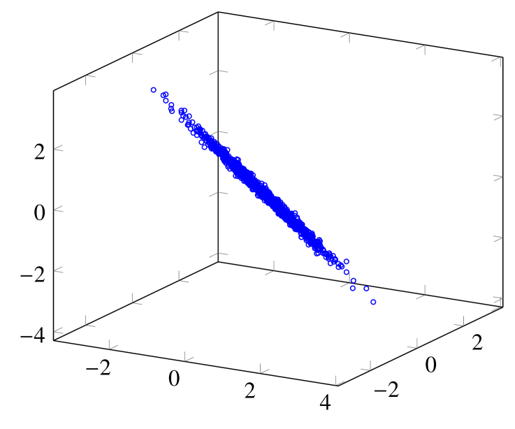
(b) $(-0.5,-0.5,-0.5)$.

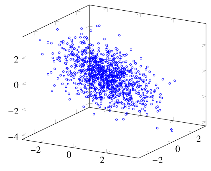
(c) $(0.1,0.1,-0.9)$.

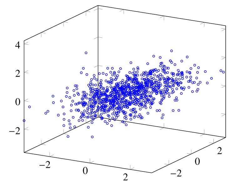
(d) $(0.7,0.5,0)$.

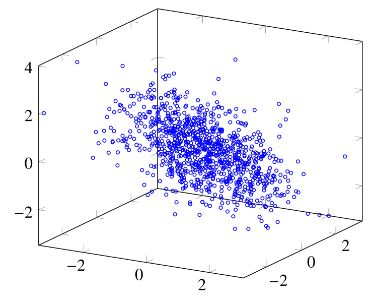
(e) $(0.2,-0.8,0)$.

(f) $(-0.3,-0.3,-0.3)$.

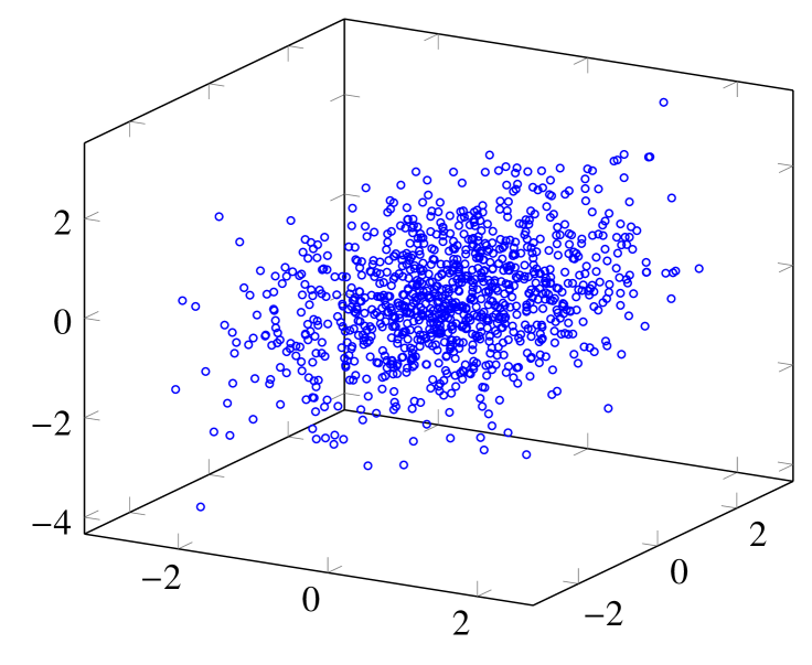
(g) $(0.2,0.3,0.4)$.

(h) $(-0.1,-0.1,0.2)$.

Figure 8.1: Scatterplots: Random samples of size $n=1000$ are drawn from the the trivariate normal distributions $\mathcal{N}_{3}(\mathbf{0},{\mathrel{\mathchoice{\ooalign{$\displaystyle\mathbf{\Sigma}$\cr\hfil$\displaystyle|$\hfil\cr}}{\ooalign{$\textstyle\mathbf{\Sigma}$\cr\hfil$\textstyle|$\hfil\cr}}{\ooalign{$\scriptstyle\mathbf{\Sigma}$\cr\hfil$\scriptstyle|$\hfil\cr}}{\ooalign{$\scriptscriptstyle\mathbf{\Sigma}$\cr\hfil$\scriptscriptstyle|$\hfil\cr}}}}_{3}(\boldsymbol{\rho}))$ for various correlation values of $\boldsymbol{\rho}=(\rho_{12},\rho_{13},\rho_{23})$.

8.1.2.   Non-normal cases

We simulate $r=1000$ random samples of size $n$ from some trivariate Archimedean copulas (Clayton, Frank, Gumbel and Joe) as well the non-Archimedean copula Farlie-Gumbel-Morgenstern (F-G-M). For the parameters of these Archimedean copulas see the R-package ‘copula’ (see, also, Brechmann and Schepsmeier, 2013); regarding data generation from the F-G-M copula see Section I of the Supplementary Material. Based on these samples we compute the averages (and the Monte Carlo mean square error) of $\hat{I}$ and $\hat{I}^{*}$; Tables 8.2 and 8.3 present the results for the Archimedean and F-G-M copula cases respectively; note that the copulas $C_{\theta}$ or $C_{-\theta}$, $\theta\in[0,1]$, see (I.1a), produce the same value of the index $I$, and so the index $I^{*}$ [the same is true for the copulas $\tilde{C}_{\theta}$ or $\tilde{C}_{-\theta}$, $\theta\in[0,1]$, see (I.1a)]. For all cases the results again empirically verify the consistency of the estimation for both $\hat{I}$ and $\hat{I}^{*}$ estimators. Figure 8.1 presents illustrations of graphs of a single sample $\{\boldsymbol{X}_{1},\ldots,\boldsymbol{X}_{n}\}$ of size $n=1000$ drawn from these distributions. The standardized index $I^{*}$ indicates that the Archimedean copulas $\mathrm{Clayton}\{2\}$, $\mathrm{Frank}\{4\}$, $\textrm{Gumbel}\{2\}$ and $\mathrm{Joe}\{2\}$ have a strong dependence level, while those corresponding to $\mathrm{Clayton}\{5\}$, $\mathrm{Frank}\{8\}$, $\textrm{Gumbel}\{4\}$ and $\mathrm{Joe}\{5\}$ have a very strong dependence level.

Table 8.2: Monte Carlo averages (and associated mean square error) of $I$ and $I^{*}$; the number of Monte Carlo repetitions is $r=1000$. Random samples of size $n$ are drawn from different Clayton, Frank, Gumbel and Joe Archimedean copulas, for various values of $n$. For each case, the parameter is shown in curly brackets, and the true values of $I$ and $I^{*}$ are denoted in the caption.

(a) $\mathrm{Clayton}\{2\}$; $I=0.362$, $I^{*}=0.715$.

	$n$
	100	$200$	$500$	$1000$
$\hat{I}_{n}$	.315(.003)	.332(.001)	.348(.000)	.354(.000)
$\hat{I}^{*}_{n}$	.637(.008)	.666(.003)	.694(.001)	.703(.000)

(b) $\mathrm{Clayton}\{5\}$; $I=0.528$, $I^{*}=0.903$.

	$n$
	100	$200$	$500$	$1000$
$\hat{I}_{n}$	.442(.008)	.479(.003)	.507(.001)	0.517(.000)
$\hat{I}^{*}_{n}$	.821(.007)	.860(.002)	.886(.000)	0.893(.000)

(c) $\mathrm{Frank}\{4\}$; $I=0.263$, $I^{*}=0.543$.

	$n$
	100	$200$	$500$	$1000$
$\hat{I}_{n}$	.241(.001)	.247(.001)	.255(.000)	.260(.000)
$\hat{I}^{*}_{n}$	.497(.000)	.510(.002)	.527(.001)	.535(.000)

(d) $\mathrm{Frank}\{8\}$; $I=0.410$, $I^{*}=0.783$.

	$n$
	100	$200$	$500$	$1000$
$\hat{I}_{n}$	.354(.004)	.378(.001)	.396(.000)	.403(.000)
$\hat{I}^{*}_{n}$	.702(.007)	.739(.002)	.764(.001)	.774(.000)

(e) $\textrm{Gumbel}\{2\}$; $I=0.361$, $I^{*}=0.714$.

	$n$
	100	$200$	$500$	$1000$
$\hat{I}_{n}$	.316(.003)	.333(.001)	.348(.000)	.354(.000)
$\hat{I}^{*}_{n}$	.638(.007)	.668(.003)	.693(.001)	.703(.000)

(f) $\textrm{Gumbel}\{4\}$; $I=0.562$, $I^{*}=0.925$.

	$n$
	100	$200$	$500$	$1000$
$\hat{I}_{n}$	.471(.008)	.509(.003)	.539(.001)	.550(.000)
$\hat{I}^{*}_{n}$	.853(.006)	.887(.002)	.910(.000)	.918(.000)

(g) $\mathrm{Joe}\{2\}$; $I=0.267$, $I^{*}=0.549$.

	$n$
	100	$200$	$500$	$1000$
$\hat{I}_{n}$	.240(.001)	.248(.001)	.258(.000)	.262(.000)
$\hat{I}^{*}_{n}$	.495(.005)	.512(.003)	.532(.001)	.540(.000)

(h) $\mathrm{Joe}\{5\}$; $I=0.496$, $I^{*}=0.876$.

	$n$
	100	$200$	$500$	$1000$
$\hat{I}_{n}$	.416(.007)	.449(.002)	.475(.001)	.484(.000)
$\hat{I}^{*}_{n}$	.790(.008)	.829(.003)	.857(.001)	.866(.000)

(a) $\mathrm{Clayton}\{2\}$.

(b) $\mathrm{Clayton}\{5\}$.

(c) $\mathrm{Frank}\{4\}$.

(d) $\mathrm{Frank}\{8\}$.

(e) $\textrm{Gumbel}\{2\}$.

(f) $\textrm{Gumbel}\{4\}$.

(g) $\mathrm{Joe}\{2\}$.

(h) $\mathrm{Joe}\{5\}$.

Figure 8.2: Scatterplots: Random samples of size $n=1000$ are drawn from Clayton, Frank, Gumbel and Joe trivariate copulas for various values of their parameters; the parameter value is shown in curly brackets.

Table 8.3: Monte Carlo averages (and associated mean square error) of $I$ and $I^{*}$; the number of Monte Carlo repetitions is $r=1000$. Random samples of size $n$ are drawn from different F-G-M copulas given by (I.1a) or (I.1b), for various values of $\theta$ and $n$. For each case, the true values of $I$ and $I^{*}$ are denoted in the caption.

(a) $C_{0.5}$; $I=0.052$, $I^{*}=0.093$.

	$n$
	100	$200$	$500$	$1000$
$\hat{I}_{n}$	.105(.003)	.075(.001)	.059(.000)	.055(.000)
$\hat{I}^{*}_{n}$	.205(.013)	.141(.003)	.108(.001)	.100(.000)

(b) $C_{0.7}$; $I=0.073$, $I^{*}=0.136$.

	$n$
	100	$200$	$500$	$1000$
$\hat{I}_{n}$	.110(.002)	.087(.001)	.076(.000)	.074(.000)
$\hat{I}^{*}_{n}$	.220(.009)	.167(.002)	.144(.000)	.138(.000)

(c) $C_{0.9}$; $I=0.094$, $I^{*}=0.180$.

	$n$
	100	$200$	$500$	$1000$
$\hat{I}_{n}$	.123(.001)	.102(.000)	.095(.000)	.094(.000)
$\hat{I}^{*}_{n}$	.245(.006)	.198(.002)	.184(.000)	.181(.000)

(d) $C_{1}$; $I=0.104$, $I^{*}=0.203$.

	$n$
	100	$200$	$500$	$1000$
$\hat{I}_{n}$	.129(.001)	.110(.000)	.105(.000)	.104(.000)
$\hat{I}^{*}_{n}$	.257(.004)	.216(.001)	.204(.001)	.203(.000)

(e) $\tilde{C}_{0.5}$; $I=0.020$, $I^{*}=0.033$.

	$n$
	100	$200$	$500$	$1000$
$\hat{I}_{n}$	.098(.005)	.062(.001)	.037(.000)	.028(.000)
$\hat{I}^{*}_{n}$	.189(.021)	.114(.005)	.065(.001)	.049(.000)

(f) $\tilde{C}_{0.7}$; $I=0.028$, $I^{*}=0.048$.

	$n$
	100	$200$	$500$	$1000$
$\hat{I}_{n}$	.098(.004)	.063(.001)	.041(.000)	.034(.000)
$\hat{I}^{*}_{n}$	.190(.016)	.117(.003)	.074(.001)	.059(.000)

(g) $\tilde{C}_{0.9}$; $I=0.035$, $I^{*}=0.062$.

	$n$
	100	$200$	$500$	$1000$
$\hat{I}_{n}$	.099(.003)	.066(.001)	.046(.000)	.040(.000)
$\hat{I}^{*}_{n}$	.192(.012)	.121(.002)	.082(.001)	.071(.000)

(h) $\tilde{C}_{1}$; $I=0.039$, $I^{*}=0.070$.

	$n$
	100	$200$	$500$	$1000$
$\hat{I}_{n}$	.100(.002)	.067(.001)	.049(.000)	.043(.000)
$\hat{I}^{*}_{n}$	.194(.010)	.125(.002)	.088(.001)	.077(.000)

(a) $C_{0.5}$.

(b) $C_{0.7}$.

(c) $C_{0.9}$.

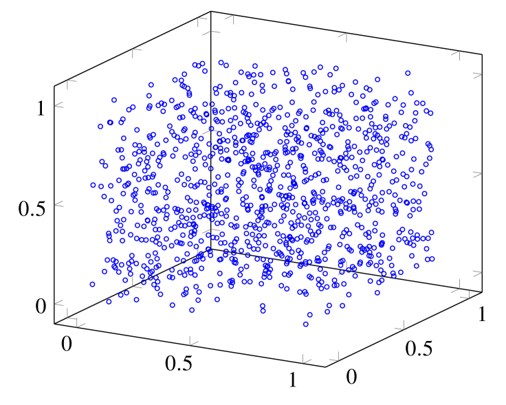
(d) $C_{1}$.

(e) $\tilde{C}_{0.5}$.

(f) $\tilde{C}_{0.7}$.

(g) $\tilde{C}_{0.9}$.

(h) $\tilde{C}_{1}$.

Figure 8.3: Scatterplots: Random samples of size $n=1000$ are drawn from different trivariate F-G-M copulas $C_{\theta}$ and $\tilde{C}_{\theta}$ for various values $\theta$, see (I.1).

General Observations: 1) As the sample size increases the bias decreases; 2) The highest percentage of bias, across all sample sizes, is observed in the case of complete dependence $(\rho_{12},\rho_{13},\rho_{23})=(1,1,1)$. In this case $I=I^{*}=1$. The observed bias (defined as $\hat{I}-I$) goes from $-26.1\%$ ($n=100$, $I$) to $-0.1\%$ ($n=1000$, $I^{*}$).

8.2.   Evaluating the proposed test of independence

We now investigate the performance of the test of independence, introduced in Section 7. Performance will be investigated in terms of both, level and power. The dimensions of the generated data are $d=2,6$. We simulate normal and non-normal data distributions. We choose to work with the bivariate case because it allows comparisons between numerical results produced and the shape of the data distributions. Figure 8.4 illustrates graphically the shape of a single random sample of size 1000 drawn from bivariate non-normal distributions we work with, with various degrees of dependence.

The results shown in Table 8.4 verify the consistency of the proposed independence test, in the bivariate normal case. As the sample size increases to infinity the power of the test increases to 1. The rate of convergence of the power to 1 depends on the strength of the association between the components of the random vector.

Table 8.4 also presents a comparison between the proposed test and the test for independence based on the estimated dHSIC statistic. We simulated this test using the R package ‘dHSIC’ by Pfister and Peters (2019). Our test exhibits higher power than the dHSIC-based test for all smaller samples and smaller values of $\rho$, while it exhibits the same power with the dHSIC-based test for larger samples and values of $\rho$.

Table 8.4: Empirical rejection rates (%) at the $\alpha=5\%$ significance level of $\mathrm{AUK}$ and dHSIC independence tests, calculated from $1000$ random samples of size $n$ simulated from $\mathcal{N}_{2}\mathopen{}\mathclose{{}\left(\boldsymbol{0},{\mathrel{\mathchoice{\ooalign{$\displaystyle\mathbf{\Sigma}$\cr\hfil$\displaystyle|$\hfil\cr}}{\ooalign{$\textstyle\mathbf{\Sigma}$\cr\hfil$\textstyle|$\hfil\cr}}{\ooalign{$\scriptstyle\mathbf{\Sigma}$\cr\hfil$\scriptstyle|$\hfil\cr}}{\ooalign{$\scriptscriptstyle\mathbf{\Sigma}$\cr\hfil$\scriptscriptstyle|$\hfil\cr}}}}_{2}(\rho)}\right)$ distribution for various values of $\rho$. The first two rows correspond to the empirical level of significance of the tests, while the other ones correspond to the empirical power of the tests.

$\rho$	test    $n$	50	100	200	300	500	750	1000	1500	2000
$0$	$\mathrm{AUK}$	$5.2$	$4.9$	$4.8$	$4.9$	$5$	$5.1$	$4.9$	$5.1$	$5$
	dHSIC	$5.5$	$5.9$	$5.1$	$4.7$	$4.3$	$4.7$	$5.5$	$5.4$	$5.2$
$0.1$	$\mathrm{AUK}$	$14.7$	$22$	$32.1$	$42.9$	$62.1$	$76.6$	$86.5$	$95.2$	$98.2$
	dHSIC	$6.8$	$8.1$	$12.7$	$15$	$24.2$	$37.9$	$48.4$	$70.3$	$80.3$
$0.2$	$\mathrm{AUK}$	$35.2$	$54.5$	$80.4$	$93.3$	$99$	$99.9$	$100$	$100$	$100$
	dHSIC	$13.2$	$23.3$	$40.1$	$59.6$	$84.4$	$95.8$	$99.3$	$100$	$100$
$0.3$	$\mathrm{AUK}$	$59.2$	$84.8$	$98.9$	$100$	$100$	$100$	$100$	$100$	$100$
	dHSIC	$27.7$	$43.3$	$80.2$	$94.8$	$99.8$	$100$	$100$	$100$	$100$
$0.4$	$\mathrm{AUK}$	$84.6$	$97.6$	$100$	$100$	$100$	$100$	$100$	$100$	$100$
	dHSIC	$46.3$	$79$	$98.1$	$99.9$	$100$	$100$	$100$	$100$	$100$
$0.5$	$\mathrm{AUK}$	$95.6$	$99.9$	$100$	$100$	$100$	$100$	$100$	$100$	$100$
	dHSIC	$71$	$96.6$	$99.9$	$100$	$100$	$100$	$100$	$100$	$100$
$0.6$	$\mathrm{AUK}$	$99.4$	$100$	$100$	$100$	$100$	$100$	$100$	$100$	$100$
	dHSIC	$92.6$	$100$	$100$	$100$	$100$	$100$	$100$	$100$	$100$

(a) $\exp\{2,3,1.3\}$.

(b) $t_{5}$ with ${\mathrel{\mathchoice{\ooalign{$\displaystyle\mathbf{\Sigma}$\cr\hfil$\displaystyle|$\hfil\cr}}{\ooalign{$\textstyle\mathbf{\Sigma}$\cr\hfil$\textstyle|$\hfil\cr}}{\ooalign{$\scriptstyle\mathbf{\Sigma}$\cr\hfil$\scriptstyle|$\hfil\cr}}{\ooalign{$\scriptscriptstyle\mathbf{\Sigma}$\cr\hfil$\scriptscriptstyle|$\hfil\cr}}}}=\big{(}{1\atop 1}~{}{1\atop 4}\big{)}$.

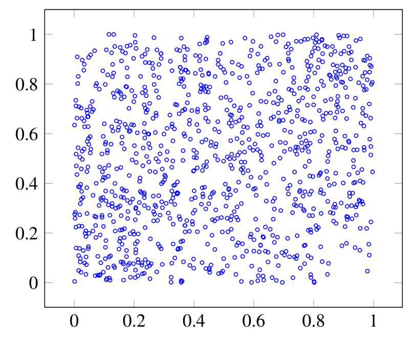
(c) $\textrm{Morgenstern}\{0.5\}$.

(d) $\textrm{Morgenstern}\{5\}$.

(e) $\textrm{Plackett}\{1.25\}$.

(f) $\textrm{Plackett}\{2\}$.

(g) $\textrm{ALI-HAQ's}\{0.1,0.5\}$.

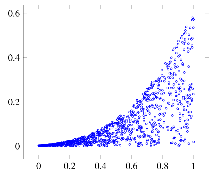
(h) $\textrm{ALI-HAQ's}\{0.9,0.5\}$.

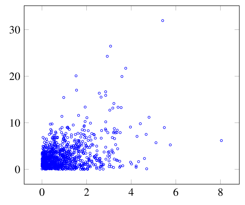
(i) $\textrm{Gumbel}\{0.9\}$.

(j) $(X,Y)$, where $(1/X,1/Y)\sim\mathcal{N}_{2}(\boldsymbol{0},I)$.

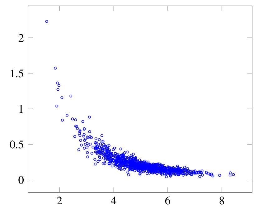
(k) $(X,\varepsilon/X^{2})$, where $X$ and $\varepsilon\sim\mathcal{N}(5,1)$ are independent.

(l) $(X,X/\varepsilon)$ with $X\sim\mathcal{N}(2,1)$, $\varepsilon\sim\mathcal{N}(5,1)$ are independent.

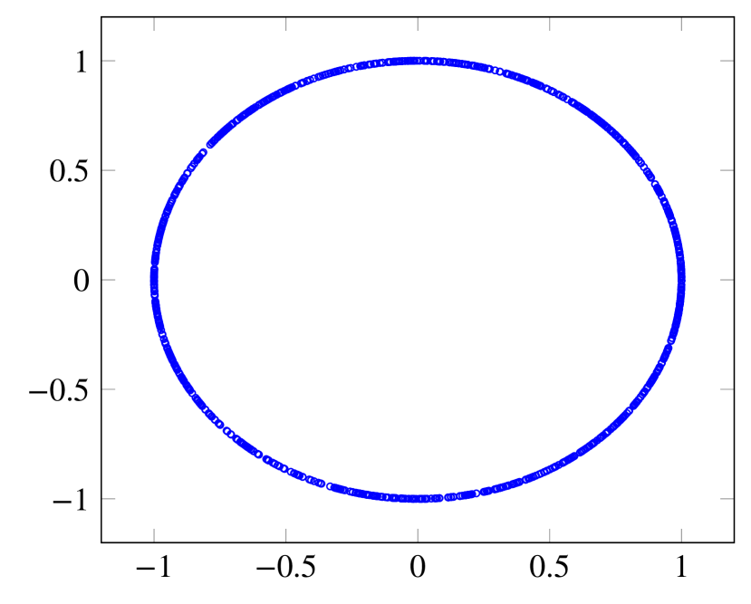
(m) $U\{C(0,1)\}$.

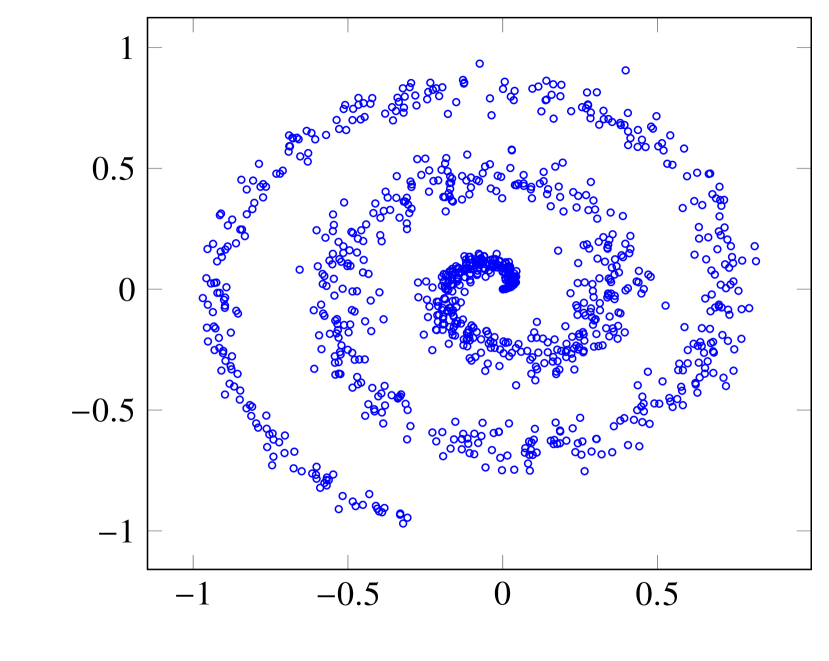
(n) Spiral data: case 1.

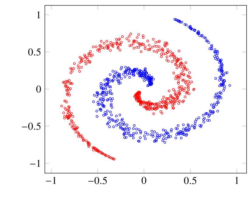
(o) Spiral data: case 2.

(p) Spiral data: case 3.

Figure 8.4: Scatter plots: Random samples of size $n=1000$ are drawn from different bivariate distributions.

In view of Table 8.5, we see that the consistency of the proposed test of independence is also verified (as the sample size increases to infinity the power of the test tends to 1).

The case $U\{C(0,1)\}$ indicates an exact cyclical dependence (see Figure 4(m)). In this case, the Kendall cdfs are $K_{i}(t)=\mathds{1}_{\{0\leq t<1/2\}}(t+1/4)+\mathds{1}_{\{1/2\leq t\leq 1\}}$ and so $\mathrm{AUK}_{i}=11/16-\ln(2)/4\approxeq 0.514$, $i=1,\ldots,4$ — see Example 7.1; hence, we compute $I=0.036$ and $I^{*}=0.074$. This kind of dependence is not recognized by both $\mathrm{AUK}$-indices. On the other hand, $\mathrm{AUK}$ is slightly different than $1/2$ and so we expect the power of the proposed test will tend to 1 as $n$ goes to infinity. Indeed, this happens even in this limited case, see the 25th row of the Table 8.5; additionally, we have that the empirical power for $n=2500$ and $3000$ is $0.941$ and $0.986$ respectively.

In view of Figure 4(j), one may incorrectly conclude that there is an association between the marginal distributions of the data distribution. Since $(1/X,1/Y)\sim\mathcal{N}_{2}(\boldsymbol{0},I)$, $X$ and $Y$ are independent continuous rvs. Thus, the rate of rejection of the null hypothesis corresponds to the empirical size of the tests. For the same values of $n$ as in Table 8.5, the empirical size of the $\mathrm{AUK}$ independence test calculated from 1000 random samples of size $n$ results in the following values 0.060, 0.053, 0.060, 0.052, 0.039, 0.052, 0.057, 0.054 and 0.046, that is, the test maintains the nominal level well for all sample sizes; notice that the dHSIC independence test also maintains the nominal level well for all sample sizes.

Table 8.5 presents the empirical power of our proposed test, as well as that of the dHSIC-based test for a variety of sample sizes and distributions. We observe that for distributions, such as $t_{5}$ with the reported covariance matrix, $\textrm{Morgenstern}\{0.5\}$, $\textrm{Plackett}\{1.25\}$ or $\textrm{Plackett}\{2\}$ our proposed test outperforms the dHSIC-based test for smaller samples and it has the same power with dHSIC-based test for larger samples. The case where the dHSIC-based test outperforms our test in terms of power is when the data come from $\textrm{ALI-HAQ's}\{0.1,0.5\}$, $U\{C(0,1)\}$ and spiral data cases 1 and 3. Hence, overall the proposed test either performs competitively or outperforms the kernel-based tests in most of the cases met in practice.

Table 8.5: Empirical power (%) of $\mathrm{AUK}$ and dHSIC independence tests, with a nominal significance level of $\alpha=0.05$, calculated from $1,000$ random samples of size $n$ simulated from various bivariate non-normal distributions.

distribution	test    $n$	50	100	200	300	500	750	1000	1500	2000
$\exp\{2,3,1.3\}$	$\mathrm{AUK}$	$97.3$	$100$	$100$	$100$	$100$	$100$	$100$	$100$	$100$
	dHSIC	$90.5$	$99.9$	$100$	$100$	$100$	$100$	$100$	$100$	$100$
$t_{5}$ with ${\mathrel{\mathchoice{\ooalign{$\displaystyle\mathbf{\Sigma}$\cr\hfil$\displaystyle|$\hfil\cr}}{\ooalign{$\textstyle\mathbf{\Sigma}$\cr\hfil$\textstyle|$\hfil\cr}}{\ooalign{$\scriptstyle\mathbf{\Sigma}$\cr\hfil$\scriptstyle|$\hfil\cr}}{\ooalign{$\scriptscriptstyle\mathbf{\Sigma}$\cr\hfil$\scriptscriptstyle|$\hfil\cr}}}}=\big{(}{1\atop 1}~{}{1\atop 4}\big{)}$	$\mathrm{AUK}$	$93.4$	$99.9$	$100$	$100$	$100$	$100$	$100$	$100$	$100$
	dHSIC	$76.9$	$97.3$	$100$	$100$	$100$	$100$	$100$	$100$	$100$
$\textrm{Morgenstern}\{0.5\}$	$\mathrm{AUK}$	$27.4$	$42.7$	$66.1$	$82.1$	$95.8$	$99$	$99.9$	$100$	$100$
	dHSIC	$16.6$	$28.1$	$50.4$	$69.7$	$87.9$	$97.9$	$99.6$	$100$	$100$
$\textrm{Morgenstern}\{5\}$	$\mathrm{AUK}$	$100$	$100$	$100$	$100$	$100$	$100$	$100$	$100$	$100$
	dHSIC	$100$	$100$	$100$	$100$	$100$	$100$	$100$	$100$	$100$
$\textrm{Plackett}\{1.25\}$	$\mathrm{AUK}$	$11.4$	$14.1$	$22.9$	$29.5$	$40.3$	$53.2$	$68.7$	$82$	$90.5$
	dHSIC	$6.3$	$10$	$15.6$	$19.7$	$26.8$	$40.4$	$48.9$	$67.9$	$80.1$
$\textrm{Plackett}\{2\}$	$\mathrm{AUK}$	$46.8$	$70.4$	$92.1$	$98.7$	$99.9$	$100$	$100$	$100$	$100$
	dHSIC	$29.6$	$57.2$	$86.9$	$96.4$	$99.8$	$100$	$100$	$100$	$100$
$\textrm{ALI-HAQ's}\{0.1,0.5\}$	$\mathrm{AUK}$	$17.2$	$26.3$	$39$	$51.7$	$69$	$84.6$	$92.4$	$99.1$	$100$
	dHSIC	$16.1$	$30.7$	$66.8$	$89.2$	$99.4$	$100$	$100$	$100$	$100$
$\textrm{ALI-HAQ's}\{0.9,0.5\}$	$\mathrm{AUK}$	$100$	$100$	$100$	$100$	$100$	$100$	$100$	$100$	$100$
	dHSIC	$100$	$100$	$100$	$100$	$100$	$100$	$100$	$100$	$100$
$\textrm{Gumbel}\{0.9\}$	$\mathrm{AUK}$	$22.1$	$35.3$	$52.6$	$68.1$	$85.9$	$95.4$	$98.7$	$100$	$100$
	dHSIC	$24.9$	$43.7$	$76.1$	$90.4$	$99.2$	$100$	$100$	$100$	$100$
$(X,\varepsilon/X^{2})$	$\mathrm{AUK}$	$100$	$100$	$100$	$100$	$100$	$100$	$100$	$100$	$100$
see Figure 4(k)	dHSIC	$100$	$100$	$100$	$100$	$100$	$100$	$100$	$100$	$100$
$(X,X/\varepsilon)$	$\mathrm{AUK}$	$100$	$100$	$100$	$100$	$100$	$100$	$100$	$100$	$100$
see Figure 4(l)	dHSIC	$100$	$100$	$100$	$100$	$100$	$100$	$100$	$100$	$100$
$U\{C(0,1)\}$	$\mathrm{AUK}$	$0$	$0.2$	$1.1$	$3.1$	$9.3$	$16.0$	$36.9$	$69$	$86.1$
	dHSIC	$96.7$	$100$	$100$	$100$	$100$	$100$	$100$	$100$	$100$
Spiral data: case 1	$\mathrm{AUK}$	$14.5$	$22.9$	$35.6$	$44.9$	$60.5$	$76$	$86.7$	$95.4$	$98.8$
	dHSIC	$28.6$	$58.5$	$93.7$	$99.2$	$100$	$100$	$100$	$100$	$100$
Spiral data: case 2	$\mathrm{AUK}$	$19.6$	$36.8$	$57.2$	$71.8$	$89.8$	$97.8$	$99.8$	$100$	$100$
	dHSIC	$10.5$	$19$	$41.4$	$69.1$	$95.3$	$99.9$	$100$	$100$	$100$
Spiral data: case 3	$\mathrm{AUK}$	$8.2$	$7.5$	$11.2$	$18.5$	$23.7$	$33.9$	$44.5$	$58.9$	$70.4$
	dHSIC	$6.8$	$14.5$	$35.7$	$62.1$	$94.2$	$100$	$100$	$100$	$100$

Table 8.6 provides the time, in seconds, needed to compute our $\mathrm{AUK}$-based and the dHSIC-based tests of independence. This table, clearly shows that the $\mathrm{AUK}$-based test is very fast to compute, requiring, for example, for sample sizes 2000 and dimension 2 only 0.048 sec.

Table 8.6: Speed time (in seconds) of the test-procedures $\mathrm{AUK}$ and dHSIC for testing the total independence of a two-variable data set of size $n$.

$n$	200	300	500	750	1000	1250	1500	1750	2000
$\mathrm{AUK}$ test	0.000	0.000	$0.015$	$0.016$	$0.017$	$0.031$	$0.032$	$0.047$	$0.048$
dHSIC test	0.609	1.500	$4.633$	$10.017$	$19.814$	$33.800$	$56.782$	$72.949$	$113.030$

9.   A real data example

Alanine and aspartate aminotransferase, ALT and AST respectively, are markers of liver inflammation. Further, alkaline phosphatase (AP), as well as direct bilirubin (DB) are biomarkers of hepatic injury, measuring inflammation from viral, metabolic or autoimmune causes. Elevation of ALT and AST is referred to as hepatocellular liver injury pattern. In contrast, alkaline phosphatase and bilirubin are increased under conditions that lead to damage of the bile ducts that drain the liver and is referred to as cholestatic injury pattern. These parameters can be elevated due to bile duct obstruction by a stone or tumor or in the case of autoimmune diseases, in which body’s immune system can attack the cholangiocytes. There can also be a mixed hepatocellular and cholestatic pattern. In the evaluation of liver disease, the pattern of injury guides the clinician toward the potential etiology and assists in directing the etiologic evaluation. Table IV.1 of the Supplementary Material presents a data set that contains measurements of (DB, AST, ALT, AP) on 208 patients with liver disease.

We estimate the indices $I$ and $I^{*}$ of the biomarkers’ vector as $\hat{I}_{208}(\mathrm{DB},\mathrm{AST},\mathrm{ALT},\mathrm{AP})=0.2546$ and $\hat{I}^{*}_{208}(\mathrm{DB},\mathrm{AST},\mathrm{ALT},\mathrm{AP})=\varphi_{4}(0.2546)\approxeq 0.561$, where the approximate polynomial $\varphi_{4}$ has been find by applying Algorithm 4.1. According to Definition 4.1, we conclude that the random vector of the biomarkes DB, AST, ALT and AP has a strong mutual dependence at the level $56.1\%$.

We next investigate the dependence structure of the random vector of these biomarkes. To accomplish this goal, we compute the indices $\hat{I}_{n}$ and $\hat{I}^{*}_{n}$ for all 2- and 3-dimensional sub-vectors of the vector of these biomarkers; Tables 1(a) and 1(b) present these results. According to Definition 4.1, we extract the following conclusions. Both $(\mathrm{DB,AST,ALT})$ and $(\mathrm{AST,ALT,AP})$ have strong mutual dependence of level $65.1\%$ and $60.5\%$ respectively, $(\mathrm{DB,AST,AP})$ has a mild mutual dependence of level $29.4\%$ and $(\mathrm{DB,ALT,AP})$ has a weak mutual dependence of level $23.2\%$; for the bidimensional sub-vectors, we have that $(\mathrm{AST,ALT})$ has a very strong mutual dependence of level $79.2\%$, $(\mathrm{DB,AST})$ has a mild mutual dependence of level $35.4\%$, and $(\mathrm{DB,ALT})$, $(\mathrm{DB,AP})$, $(\mathrm{AST,AP})$ and $(\mathrm{ALT,AP})$ have weak mutual dependence of level $23\%$, $20.4\%$, $17.1\%$ and $14.2\%$ respectively. In addition to the indices $\hat{I}$ and $\hat{I}^{*}$, Table 1(a) presents the corresponding sample Kendall’s $\tau$ correlation coefficients. We observe that $\hat{I}^{*}$ and $\hat{\tau}$ recognize an association between two biomarkers almost in a similar way but, in general, the index $\hat{I}^{*}$ indicates a stronger dependence level. Notice that Kendall’s $\tau$ correlation coefficient cannot be used beyond the bivariate case.

The strong dependence between AST and ALT can be explained from the physiological point of view, since they are both released when hepatocytes undergo cell death. On the other hand, the weak dependence among the pairs of biomarkers can be explained by the fact that there are released under different mechanisms. When evaluating three biomarkers simultaneously, we identify the strongest dependency among the triplet $(\mathrm{DB,AST,ALT})$. This observation can be explained from the physiologic point of view because processes that cause hepatocyte injury would also have a likely predilection to affect hepatocyte synthetic ability. This results in the inability of hepatocyte to conjugate bilirubin, as assessed by DB. The dependence among the different biomarkers we observe can, therefore, be explained in the context of liver function and injury.

In conclusion, we say that the high level of the mutual dependence of the random vector of the biomarkers is mainly due to the very strong dependence between biomarkers AST and ALT, and secondly, to a small extent, on the dependence between the biomarkers bilirubin and AST.

Table 9.1: The estimators of the indices $\hat{I}_{n}$ and $\hat{I}^{*}_{n}$ for the 2- and 3-dimensional sub-vectors of the vector of the biomarkers DB, AST, ALT and AP.

(a) 2-dimensional sub-vectors.

	(DB, AST)	(DB, ALT)	(DB, AP)	(AST,ALT)	(AST,AP)	(ALT, AP)
$\hat{I}_{n}$	0.176	0.112	0.099	0.468	0.083	0.069
$\hat{I}^{*}_{n}$	0.354	0.230	0.204	0.792	0.171	0.142
$\hat{\tau}$	0.215	0.092	0.061	0.619	0.097	0.077

(b) 3-dimensional sub-vectors.

	(DB, AST, ALT)	(DB, AST, AP)	(DB, ALT, AP)	(AST, ALT, AP)
$\hat{I}_{n}$	0.322	0.146	0.118	0.296
$\hat{I}^{*}_{n}$	0.651	0.294	0.232	0.605

In addition to the preceding numerical results, Figures 9.1 and 9.2 shows the scatterplots of the bivariate and trivariate sub-vectors of the vector of biomarkers $(\mathrm{DB,AST,ALT,AP})$ respectively, illustrating graphically the dependence structure of these sub-vectors. Notice that even in the simplest case of bivariate random vectors it seems difficult to evaluate the strength of the dependence structure via scatterplots.

(a) $(\mathrm{DB,AST})$.

(b) $(\mathrm{DB,ALT})$.

(c) $(\mathrm{DB,AP})$.

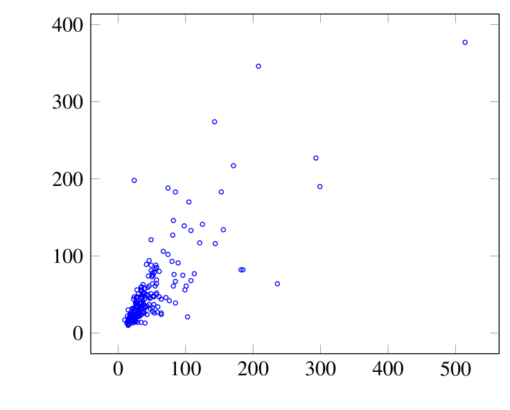
(d) $(\mathrm{AST,ALT})$.

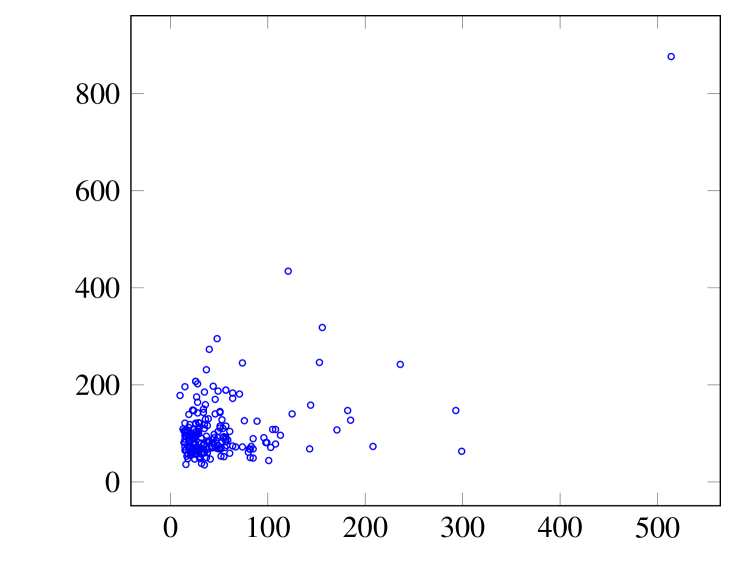
(e) $(\mathrm{AST,AP})$.

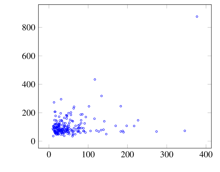
(f) $(\mathrm{ALT,AP})$.

Figure 9.1: The scatterplots of the bivariate sub-vectors of $(\mathrm{DB,AST,ALT,AP})$.

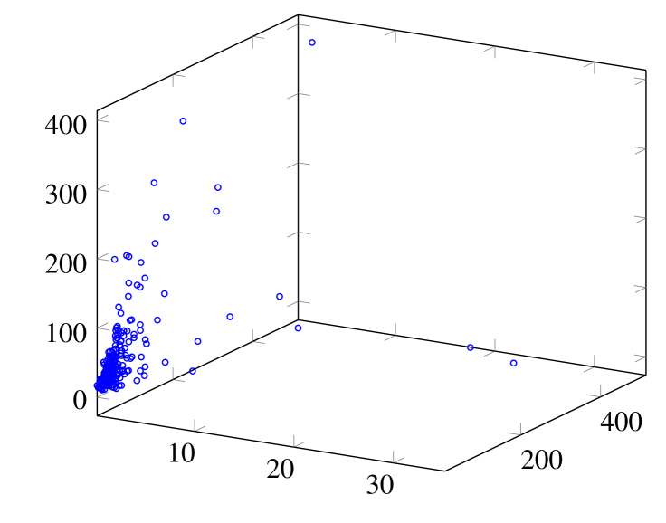
(a) $(\mathrm{DB,AST,ALT})$.

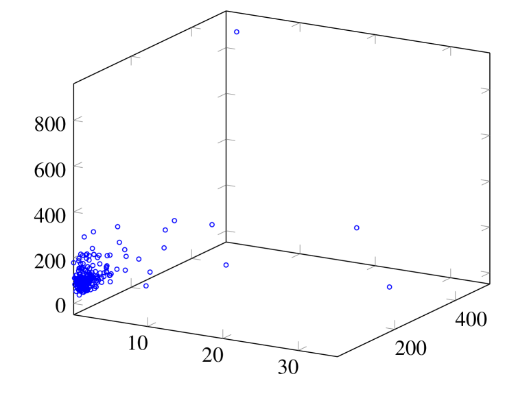
(b) $(\mathrm{DB,AST,AP})$.

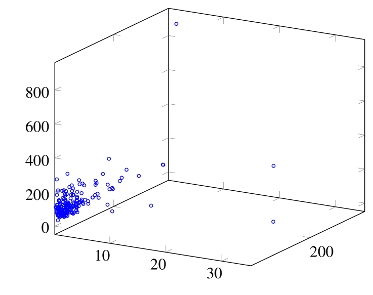
(c) $(\mathrm{DB,ALT,AP})$.

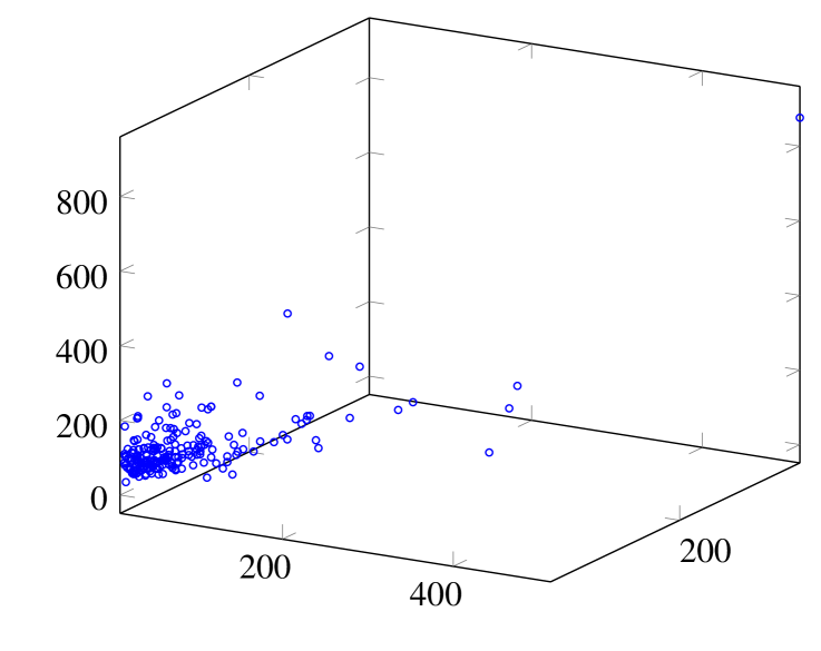
(d) $(\mathrm{AST,ALT,AP})$.

Figure 9.2: The scatterplots of the trivariate sub-vectors of $(\mathrm{DB,AST,ALT,AP})$.

10.   Concluding Remarks and Discussion

In this article we construct indices that measure joint or mutual dependence in a $d$-dimensional random vector. The indices depend on the Kendall process and satisfy the axioms set by Rényi that a function must satisfy in order to be called a measure of dependence. We evaluate the performance of the indices via simulation for a variety of distributions and sample sizes and present algorithms for their computation. Our proposed indices are copula-based and they are able to capture the degree of dependence exhibited in the data.

We also present a practical and fast, easy to compute, test for independence based on the estimated area under the Kendall curve, and propose an algorithm to compute quantities associated with its distribution.The performance of the proposed test statistic is evaluated via Monte Carlo simulation and is compared with the performance of the dHSIC-based test in terms of power and level, in a wide range of distributions and sample sizes. Our proposed test either outperforms or is competitive with the dHSIC-based test in most of the cases studied.

Appendix A Lists of axioms for dependence measures

According to Schweizer and Wolff (1981), we can present Rényi’s conditions regarding a measure of dependence $R(X,Y)$ for two continuously distributed variables $X$ and $Y$ in the following form.

1. $R(X,Y)$ is defined for any $X$ and $Y$.

2. $R(X,Y)=R(Y,X)$.

3. $0\leq R(X,Y)\leq 1$

4. $R(X,Y)=0$ if and only if $X$ and $Y$ are independent.

5. $R(X,Y)=1$ if and only if each of $X$, $Y$ is a.s. a strictly monotone function of the other.

6. If $f$ and $g$ are strictly monotone a.s. on Range $X$ and Range $Y$, respectively, then $R\{f(X),g(Y)\}=R(X,Y)$.

7. If the joint distribution of $X$ and $Y$ is bivariate normal, with correlation coefficient $\rho$, then $R(X,Y)$ is a strictly increasing function of $|\rho|$.

8. If $(X,Y)$ and $(X_{n},Y_{n})$, $n=1,2,\ldots$, are pairs of random variables with joint distributions $H$ and $H_{n}$, respectively, and if the sequence $\{H_{n}\}$ converges weakly to $H$, then $\lim_{n\to\infty}R(X_{n},Y_{n})=R(X,Y)$.

Móri and Székely (2019) propose four natural axioms for dependence measures as follows. Let $\mathpzc{S}$ be a nonempty set of pairs of nondegenerate random variables $\boldsymbol{X}$, $\boldsymbol{Y}$ taking values in Euclidean spaces or in real, separable Hilbert spaces $\mathpzc{H}$. (Nondegenerate means that the random variable is not constant with probability 1.) Then $\varDelta\colon\mathpzc{S}\to[0,1]$ is called a dependence measure on $\mathpzc{S}$ if the following four axioms hold. In the axioms below we need similarity transformations of $\mathpzc{H}$. Similarity of $\mathpzc{H}$ is defined as a bijection (1–1 correspondence) from $\mathpzc{H}$ onto itself that multiplies all distances by the same positive real number (scale). Similarities are known to be compositions of a translation, an orthogonal linear mapping, and a uniform scaling. They assume that if $(\boldsymbol{X},\boldsymbol{Y})\in\mathpzc{S}$ then $(L\boldsymbol{X},M\boldsymbol{Y})\in\mathpzc{S}$ for all similarity transformations $L$, $M$ of $\mathpzc{H}$.

1. $\varDelta(\boldsymbol{X},\boldsymbol{Y})=0$ if and only if $\boldsymbol{X}$ and $\boldsymbol{Y}$ are independent.

2. $\varDelta(\boldsymbol{X},\boldsymbol{Y})$ is invariant with respect to all similarity transformations of $\mathpzc{H}$; that is, $\varDelta(L\boldsymbol{X},M\boldsymbol{Y})=\varDelta(\boldsymbol{X},\boldsymbol{Y})$ where $L$, $M$ are similarity transformations of $\mathpzc{H}$.

3. $\varDelta(\boldsymbol{X},\boldsymbol{Y})=1$ if and only if $\boldsymbol{Y}=L\boldsymbol{X}$ with probability 1, where $L$ is a similarity transformation of $\mathpzc{H}$.

4. $\varDelta(\boldsymbol{X},\boldsymbol{Y})$ is continuous; that is, if $(\boldsymbol{X}_{n},\boldsymbol{Y}_{n})\in\mathpzc{S}$, $n=1,2,\ldots$, such that for some positive constant $K$ we have $\operatorname{\mathds{E}}(|\boldsymbol{X}_{n}|^{2}+|\boldsymbol{Y}_{n}|^{2})\leq K$, $n=1,2,\ldots$, and $(\boldsymbol{X}_{n},\boldsymbol{Y}_{n})$ converges weakly (converges in distribution) to $(\boldsymbol{X},\boldsymbol{Y})$ then $\varDelta(\boldsymbol{X}_{n},\boldsymbol{Y}_{n})\to\varDelta(\boldsymbol{X},\boldsymbol{Y})$. (The condition on the boundedness of second moments can be replaced by any other condition that guarantees the convergence of expectations: $\operatorname{\mathds{E}}(\boldsymbol{X}_{n})\to\operatorname{\mathds{E}}(\boldsymbol{X})$ and $\operatorname{\mathds{E}}(\boldsymbol{Y}_{n})\to\operatorname{\mathds{E}}(\boldsymbol{Y})$; such a condition is the uniform integrability of $\boldsymbol{X}_{n}$, $\boldsymbol{Y}_{n}$ which follows from the boundedness of second moments.)

Appendix B Kendall process

First, we state a modified empirical Kendall cdf as it is introduced by Genest and Rivest (1993), (see also Barbe et al., 1996). Let $\tilde{T}_{ni}=\{\#j\neq i\colon\boldsymbol{X}_{j}\leq\boldsymbol{X}_{i}\textrm{ componentwise}\}/(n-1)$. Denote by $\tilde{\mathbb{K}}_{n}$ the empirical distribution function of the $\tilde{T}_{ni}$’s that is an empirical Kendall cdf, i.e. an estimator of the Kendall cdf $K$.

We state now the following hypotheses.

1. The Kendall cdf $K(t)$ admits a continuous probability density function $k(t)$ on $(0,1]$ that verifies $k(t)=o\{t^{-1/2}\ln^{-1/2-\varepsilon}(1/t)\}$ for some $\varepsilon>0$ as $t\to 0$.

2. There exists a version of the conditional distribution of the vector $(F_{1}(X_{1}),\ldots,F_{d}(X_{d}))$ given $T=t$ and a countable family $\mathcal{P}$ of partitions $\mathcal{C}$ of $[0,1]^{d}$ into a finite number of Borel sets satisfying

   $$\inf_{\mathcal{C}\in\mathcal{P}}\max_{C\in\mathcal{C}}\mathrm{diam}(C)=0,$$

   such that for all $C\in\mathcal{C}$, the mapping $t\mapsto\mu_{t}(C)=k(t)\operatorname{\mathds{P}}\{(F_{1}(X_{1}),\ldots,F_{d}(X_{d}))\in C|T=t\}$ is continuous on $(0,1]$ with $\mu_{1}(C)=k(1)\mathds{1}_{\{(1,\ldots,1)\in C\}}$.

Given $0\leq s,t\leq 1$, define

$$Q(s,t)=\operatorname{\mathds{P}}\{F(\boldsymbol{X}_{1})\leq s,\boldsymbol{X}_{1}\leq\boldsymbol{X}_{2}|F(\boldsymbol{X}_{2})=t\}-tK(s)$$

and

$$R(s,t)=\operatorname{\mathds{P}}\{\boldsymbol{X}_{1}\leq\boldsymbol{X}_{2}\wedge\boldsymbol{X}_{3}|F(\boldsymbol{X}_{2})=s,H(\boldsymbol{X}_{3})=t\}-st,$$

where $\boldsymbol{X}_{1},\ldots,\boldsymbol{X}_{3}$ are independent and identically distributed random vectors from $F$, and $\boldsymbol{u}\wedge\boldsymbol{v}$ denotes the componentwise minimum between $\boldsymbol{u}$ and $\boldsymbol{v}$.

Consider now the Kendall process $\mathbb{G}_{n}(t)\doteq\surd{n}\{\tilde{\mathbb{K}}_{n}(t)-K(t)\}$, $0\leq t\leq 1$. The following result is given by Barbe et al. (1996, Theo. 1), (cf. Genest and Rivest, 1993; Wellner, 2005; Salvadori et al., 2013).

Theorem B.1.

Under $\mathrm{H}_{1}$ and $\mathrm{H}_{2}$, the Kendal process $\mathbb{G}_{n}(t)=\surd{n}\{\tilde{\mathbb{K}}_{n}(t)-K(t)\}$, $0\leq t\leq 1$ converges in distribution to a Gaussian process $\mathbb{G}_{K}$ with zero mean and covariance function

$$\varGamma(s,t)=K(s\wedge t)-K(s)K(t)+k(s)k(t)R(s,t)-k(t)Q(s,t)-k(s)Q(t,s).$$

We restate here the hypothesis test $H_{0}\colon F=\prod_{j=1}^{d}F_{j}$ versus $H_{1}\colon F\neq\prod_{j=1}^{d}F_{j}$. Under $H_{0}$, $K_{H_{0}}=K_{\varPi}$ and $k_{H_{0}}=k_{\varPi}$; additionally, (see Barbe et al., 1996, Example 1, p. 202),

$$\surd{n}\{\tilde{\mathbb{K}}_{n}(t)-K_{\varPi}(t)\}\stackrel{{\scriptstyle H_{0}}}{{\rightsquigarrow}}\mathbb{G}_{\varPi},$$ (B.1)

where $\mathbb{G}_{\varPi}$ is a Gaussian process with zero mean and for $0\leq s,t\leq 1$ covariance function as it given by (7.2). In (7.2b) we have corrected a minor misprint (see Barbe et al., 1996, p. 208, for the correct general formula). Relations (7.2) lead to a cumbersome but explicit expression for the covariance function $\varGamma_{\varPi}$, which reduces to $\varGamma_{\varPi}(s,t)=s(t-1-\ln t)$, $0\leq s\leq t\leq 1$, when $d=2$.

A $\tilde{\mathbb{K}}_{n}$-based estimator of $\mathrm{AUK}$ is $\tilde{\mathrm{AUK}}_{n}=\operatorname{\mathds{E}}\mathopen{}\mathclose{{}\left\{1-K_{\varPi}(\tilde{T}_{n})}\right\}=1-n^{-1}\sum_{i=1}^{n}K_{\varPi}(\tilde{T}_{ni})$. Hence, using functional delta-method, we get $\surd{n}(\tilde{\mathrm{AUK}}_{n}-1/2)\stackrel{{\scriptstyle H_{0}}}{{\rightsquigarrow}}\mathcal{N}(0,\sigma_{\varPi}^{2})$, where $\sigma_{\varPi}^{2}$ is defined by (7.1b). When $d=2$, after a straightforward calculation, we compute $\sigma_{\varPi}^{2}=19/423$. For completing the proof of (7.1) it is sufficient to prove that $\surd{n}(\hat{\mathrm{AUK}}_{n}-\tilde{\mathrm{AUK}}_{n})=o_{p}(1)$ as $n\to\infty$. For the proof of the asymptotic normality of both $\tilde{\mathrm{AUK}}$ and $\hat{\mathrm{AUK}}$ see Appendix D.

Appendix C Useful results

The next result is the multivariate version of Pólya’s Theorem (Shao, 2003, Prop. 1.16, p. 51). First, denote by $\|f\|_{\infty}\doteq\sup_{\boldsymbol{x}\in\mathds{R}^{d}}|f(\boldsymbol{x})|$ the supremum norm of $f\colon\mathds{R}^{d}\to\mathds{R}$.

Theorem C.1.

Let $F$ and $F_{n}$ are cdfs on $\mathds{R}^{d}$. If $F_{n}\Rightarrow F$ and $F$ is a continuous cdf, then $\|F_{n}-F\|_{\infty}\to 0$.

Theorem C.2.

Let $\boldsymbol{X}\sim F$ and $\boldsymbol{X}_{n}\sim F_{n}$ on $\mathds{R}^{d}$ such that $\boldsymbol{X}_{n}\rightsquigarrow\boldsymbol{X}$. Consider the random variables $T\doteq F(\boldsymbol{X})$ and $T_{n}\doteq F_{n}(\boldsymbol{X}_{n})$. If $F$ is continuous, $T_{n}\rightsquigarrow T$.

Proof.

By Skorokhod’s representation Theorem, there are $\tilde{\boldsymbol{X}}$ and $\tilde{\boldsymbol{X}}_{n}$ defined in the same probability space $(\varOmega,\mathcal{A},\operatorname{\mathds{P}})$ such that $\check{\boldsymbol{X}}\sim F$, $\check{\boldsymbol{X}}_{n}\sim F_{n}$ and

$$\check{\boldsymbol{X}}_{n}(\omega)\to\check{\boldsymbol{X}}(\omega)\quad\textrm{for each}\ \omega\in\varOmega,$$ (C.1)

(see, for example, Billingsley, 2013, Theo. 25.6). Consider now the random variables $\check{T}\doteq F(\check{\boldsymbol{X}})$ and $\check{T}_{n}\doteq F_{n}(\check{\boldsymbol{X}}_{n})$; then, applying the triangle inequality, for each $\omega\in\varOmega$,

$$|\check{T}_{n}(\omega)-\check{T}(\omega)|\leq|F_{n}\{\check{\boldsymbol{X}}_{n}(\omega)\}-F\{\check{\boldsymbol{X}}_{n}(\omega)\}|+|F\{\check{\boldsymbol{X}}_{n}(\omega)\}-F\{\check{\boldsymbol{X}}(\omega)\}|.$$

Because of continuity of $F$, (C.1) implies that

$$|F\{\check{\boldsymbol{X}}_{n}(\omega)\}-F\{\check{\boldsymbol{X}}(\omega)\}|\to 0.$$

Using Theorem C.1, for each $\omega\in\varOmega$,

$$|F_{n}\{\check{\boldsymbol{X}}_{n}(\omega)\}-F\{\check{\boldsymbol{X}}_{n}(\omega)\}|\leq\|F_{n}-F\|_{\infty}\to 0.$$

Consequently, $\check{T}_{n}(\omega)\to\check{T}(\omega)$ for each $\omega\in\varOmega$; this implies that $\check{T}_{n}\xlongrightarrow{\textrm{\begin{picture}(0.0,0.0)\put(0.0,0.0){\makebox(-1.75,-0.5)[]{$\mathrm{as}$}}\end{picture}}}\check{T}$ which gives $\check{T}_{n}\rightsquigarrow\check{T}$, and so $T_{n}\rightsquigarrow T$. ∎

From Theorem C.2 and Faugeras (2013, Theo. 3.1, p. 274) the following theorem follows.

Theorem C.3.

Let $\boldsymbol{X}\sim F$ and $T$ as in Theorem C.1, and $\{\boldsymbol{X}_{n}\}$ be an independent and identically distributed sequence from $F$. Consider the sequences of the ecdfs $\mathbb{F}_{n}$ as well as its empirical Kendall distribution functions $\mathbb{K}_{n}$. If $\hat{T}_{n}\sim\mathbb{K}_{n}$, then $\hat{T}_{n}\rightsquigarrow T$.

Appendix D Proofs of the main manuscript

Proof of Equation (4.2).

Suppose $Y$ is a continuous rv and consider the $d$-dimensional rvs $\boldsymbol{Y}^{(1)}=(Y,\ldots,Y)$ and $\boldsymbol{Y}^{(2)}=(Y,\ldots,Y,-Y,\ldots,-Y)^{T}$ (the first $p\geq 1$ components of $\boldsymbol{Y}^{(2)}$ are $Y$ and the last $d-p\geq 1$ are $-Y$). For each $\boldsymbol{y}=(y_{1},\dots,y_{d})^{T}\in\mathds{R}^{d}$, one can easily see that $F_{\boldsymbol{Y}^{(1)}}(\boldsymbol{y})=\operatorname{\mathds{P}}(Y\leq\min\{y_{1},\ldots,y_{d}\})$; consequently, $T_{\boldsymbol{Y}^{(1)}}=F_{\boldsymbol{Y}^{(1)}}(\boldsymbol{Y}^{(1)})=F_{Y}(Y)\sim U(0,1)$, and so $K_{\boldsymbol{Y}^{(1)}}(t)=t$, $t\in[0,1]$. The $\mathrm{AUK}$ is

$$\mathrm{AUK}_{\boldsymbol{Y}^{(1)}}=\int_{0}^{1}t\frac{(-\ln t)^{d-1}}{(d-1)!}\operatorname{d\textrm{$t$}}=2^{-d}\int_{0}^{\infty}\frac{2^{d}}{(d-1)!}x^{d-1}e^{-2x}\operatorname{d\textrm{$x$}}=2^{-d}.$$

In the case of $\boldsymbol{Y}^{(2)}$, we can easily to verify $F_{\boldsymbol{Y}^{(2)}}(\boldsymbol{y})=\operatorname{\mathds{P}}(\max\{-y_{p+1},\ldots,-y_{d}\}\leq Y\leq\min\{y_{1},\ldots,y_{p}\})=\max\{0,F_{Y}(\min\{y_{1},\ldots,y_{p}\})-F_{Y}(\max\{-y_{p+1},\ldots,-y_{d}\})\}$; therefore, $T_{\boldsymbol{Y}^{(2)}}=\max\{0,F_{Y}(Y)-F_{Y}(Y)\}=0$ with probability one, and so $K_{\boldsymbol{Y}^{(2)}}(t)=1$, $t\in[0,1]$. Thus,

$$\mathrm{AUK}_{\boldsymbol{Y}^{(2)}}=\operatorname{\mathds{P}}(T_{\boldsymbol{Y}^{(2)}}\leq\varPi)=\operatorname{\mathds{P}}(0\leq\varPi)=1.$$

For a continuous rv $X$, consider the $d$-dimensional $\tilde{\boldsymbol{X}}=(X,\ldots,X)^{T}$. The set $\mathcal{R}(\tilde{\boldsymbol{X}})$ contains 2 rvs of the kind of $\boldsymbol{Y}^{(1)}$, specifically $(X,\ldots,X)^{T}$ and $(-X,\ldots,-X)^{T}$, and $2^{d}-2$ of the kind of $\boldsymbol{Y}^{(2)}$ (note that the coordinates of minus do not play any role). Hence, the corresponding vector $\tilde{\boldsymbol{D}}$ has 2 elements equals $2^{-d}$ and $2^{d}-2$ elements equals 1; so, $\|\tilde{\boldsymbol{D}}-\boldsymbol{\varDelta}\|=\mathopen{}\mathclose{{}\left(2^{d-2}-2^{1-d}+2^{1-2d}}\right)^{1/2}$, completing the proof. ∎

Proof of Proposition 5.1.

(a) By definition of $I$, $A_{1}$ holds in $\mathcal{X}^{d}_{0}$; while $A_{2}$ is obvious. Regarding $A_{6}$, for any such $f_{i}$s define $s^{f_{i}}=1$ if $f_{i}$ is increasing function and $-1$ when $f_{i}$ is decreasing function, and set $\boldsymbol{s}^{f}=(s^{f_{1}},\ldots,s^{f_{d}})^{T}\in\mathds{S}^{d}$, $\tilde{\boldsymbol{X}}=\operatorname{diag}(\boldsymbol{s}^{f})\boldsymbol{X}$ and $\tilde{f}_{i}(x_{i})=f_{i}(s^{f_{i}}x_{i})$, $i=1,\ldots,d$ (strictly increasing functions). Then, obviously, the random vectors $f(\boldsymbol{X})=(f_{1}(X_{1}),\ldots,f_{d}(X_{d}))^{T}$ and $\tilde{f}(\boldsymbol{X})=(\tilde{f}_{1}(X_{1}),\ldots,\tilde{f}_{d}(X_{d}))^{T}$ belong to $\mathcal{X}^{d}_{0}$ and $\mathcal{R}\{f(\boldsymbol{X})\}=\mathcal{R}\{\tilde{f}(\boldsymbol{X})\}$. Observe now that for each $\boldsymbol{s}_{j}=(s_{1j},\ldots,s_{dj})^{T}\in\mathds{S}^{d}$, $\operatorname{diag}(\boldsymbol{s}_{j})f(\boldsymbol{X})=\operatorname{diag}(\boldsymbol{s}_{j})\tilde{f}(\tilde{\boldsymbol{X}})=\tilde{f}^{(j)}\{\operatorname{diag}(\boldsymbol{s}_{j})\tilde{\boldsymbol{X}}\}$, where $\tilde{f}^{(j)}=\big{(}\tilde{f}^{(j)}_{1},\ldots,\tilde{f}^{(j)}_{d}\big{)}^{T}$ with $\tilde{f}^{(j)}_{i}(x_{i})=s_{ij}\tilde{f}_{i}(s_{ij}x_{i})$ to be an strictly increasing function for each $i=1,\ldots,d$. Hence, it becomes clear that it is enough to prove the desired result for strictly increasing functions; to prove this, one can use the similar arguments as in Vexler et al. (2019, proof of Proposition 4.4, p. 439). With regard to $A_{7}$, only for $d=2$, it has been studied by Vexler et al. (2019). Finally, suppose $\boldsymbol{X}_{n}\rightsquigarrow\boldsymbol{X}\in\mathcal{X}^{d}_{0}$. Since $K_{\varPi}(t)$, $0\leq t\leq 1$, is a continuous and bounded function, from Theorem C.2 (see Appendix C) and Portmanteau theorem we have that, for each $j=1,\ldots,2^{d}$, $\mathrm{AUK}_{nj}\to\mathrm{AUK}_{j}$, and so, $I(\boldsymbol{X}_{n})\to I(\boldsymbol{X})$; that, is $A_{8}$ holds.

(b) If $X_{1},\ldots,X_{d}$ are independent, one can easily see that $\mathrm{AUK}_{j}=0$ for all $j=1,\ldots,2^{d}$, and so $I=0$. Conversely, by definition, $I=0$ implies that $\mathrm{AUK}_{j}=0$ for all $j=1,\ldots,2^{d}$. Since $\boldsymbol{X}\in\mathcal{X}^{d}_{1}$, there is at least an subscript $j^{\prime}\in\{1,\ldots,2^{d}\}$ for which $K_{j^{\prime}}(t)=K_{\varPi}(t)$ for $0\leq t\leq 1$. Hence, from Sklar’s Theorem (see Sklar, 1959; Durante et al., 2012; Salvadori et al., 2013) the corresponding (unique) copula to $F_{\boldsymbol{X}_{j^{\prime}}}$ is the copula $\boldsymbol{C}_{0}(\boldsymbol{u})=u_{1}\cdots u_{d}$, $\boldsymbol{u}\in[0,1]^{d}$, that corresponds to the independence case. Consequently, the components of $\boldsymbol{X}_{j^{\prime}}$ are totally independent which is equivalent to the components of $\boldsymbol{X}$ are totally independent, i.e. $F_{\boldsymbol{X}}(\boldsymbol{x})=\prod_{i=1}^{d}F_{X_{i}}(x_{i})$ for all $\boldsymbol{x}\in\mathds{R}^{d}$.

(c) It is clear that $I\geq 0$ for all $\boldsymbol{X}\in\mathcal{X}^{d}_{0}$. Suppose that $\boldsymbol{X}\in\mathcal{X}^{d}_{2}$. Based on the Fréchet-Hoeffding upper-bound (see, for example, Rüschendorf, 2017), we have $K(t)=\operatorname{\mathds{P}}\{F(\boldsymbol{X})\leq t\}\geq\operatorname{\mathds{P}}\mathopen{}\mathclose{{}\left[\min_{j=1,\ldots,d}\{F_{j}(X_{j})\}\leq t}\right]\geq\operatorname{\mathds{P}}\{F_{1}(X_{1})\leq t\}=t$ for all $0\leq t\leq 1$; also, obviously, $K(t)\leq 1$ for all $0\leq t\leq 1$. Since $\boldsymbol{X}\in\mathcal{X}^{d}_{2}$, there are at least two $\boldsymbol{X}_{j^{\prime}},\boldsymbol{X}_{j^{\prime\prime}}\in\mathcal{R}(\boldsymbol{X})$ for which $\mathrm{C}_{2}$ holds; so, see in the proof of (4.2) above, $\sum_{j=j^{\prime},j^{\prime\prime}}(\mathrm{AUK}_{j}-1/2)^{2}\leq 2(1-2^{-d})^{2}$. On the other hand, it is obvious that $\sum_{j\neq j^{\prime},j^{\prime\prime}}(\mathrm{AUK}_{j}-1/2)^{2}\leq(2^{d}-2)/4$. Hence, $\sum_{j}(\mathrm{AUK}_{j}-1/2)^{2}\leq 2^{d-2}-2^{1-d}+2^{1-2d}$, which implies that $I\leq 1$. Suppose now $\boldsymbol{X}\in\mathcal{X}^{d}_{2}$ with $I=1$. Then, there is a subscript $j^{\prime}$ such that $K_{j^{\prime}}(t)=t$, $0\leq t\leq 1$. As in (b), from Sklar’s Theorem the corresponding (unique) copula to $F_{\boldsymbol{X}_{j^{\prime}}}$ is the copula $\boldsymbol{C}_{1}(\boldsymbol{u})=\min\{u_{1},\ldots,u_{d}\}$, $\boldsymbol{u}\in[0,1]^{d}$, that corresponds to the total dependence case. ∎

Proof of Proposition 5.2.

(a) See Proposition 5.1b. (b) See Proposition 5.1a. (c) Similar to Proposition 5.1c. ∎

Proof of Proposition (6.2).

Suffice it to prove the result for the original (non-rotated) data. Set $D_{n}\doteq\|\mathbb{F}_{n}-F\|_{\infty}$. The multivariate version of Dvoretzky-Kiefer-Wolfowitz inequality says that (see Kiefer, 1961, Eq. (1.2), p. 649), there are positive constants $c^{\prime}_{d}$ and $c_{d}$ (do not depend on $F$) such that, $\operatorname{\mathds{P}}(D_{n}>z)\leq c^{\prime}_{d}\exp(-c_{d}nz^{2})$ for all $n>0$ and $z\geq 0$. For $\epsilon>0$, set $\theta_{\epsilon}=\exp(-c_{d}\epsilon^{2})\in(0,1)$; then,

$$\operatorname{\mathds{P}}\mathopen{}\mathclose{{}\left(\sup_{m\geq n}D_{m}>\epsilon}\right)\leq\sum_{m=n}^{\infty}\operatorname{\mathds{P}}(D_{m}>\epsilon)\leq c^{\prime}_{d}\sum_{m=n}^{\infty}\theta_{\epsilon}^{m}=\frac{c^{\prime}_{d}}{1-\theta_{\epsilon}}\theta_{\epsilon}^{n}\to 0,\textrm{ as }n\to\infty.$$

Therefore, the multivariate version of Glivenko-Cantelli Theorem follows, that is,

$$\|\mathbb{F}_{n}-F\|_{\infty}\xlongrightarrow{\textrm{\begin{picture}(0.0,0.0)\put(0.0,0.0){\makebox(-1.75,-0.5)[]{$\mathrm{as}$}}\end{picture}}}0.$$

Consider $\xi(\boldsymbol{x})\doteq K_{\varPi}\{F(\boldsymbol{x})\}$ and $\hat{\xi}_{n}(\boldsymbol{x})\doteq K_{\varPi}\{\mathbb{F}_{n}(\boldsymbol{x})\}$. Since $K_{\varPi}$ is a continuous and bounded function, from the preceding result we have that $\hat{\xi}_{n}$ convergence almost surely to $\xi$ (uniformly). Let $P$ and $\mathbb{P}_{n}$ denote the probability measures that correspond to $F$ and $\mathbb{F}_{n}$ respectively. Because of bounding of $\xi$, $\hat{\mathrm{AUK}}=\int\hat{\xi}_{n}\operatorname{d\textrm{$\mathbb{P}_{n}$}}\xlongrightarrow{\textrm{\begin{picture}(0.0,0.0)\put(0.0,0.0){\makebox(-1.75,-0.5)[]{$\mathrm{as}$}}\end{picture}}}\int\xi\operatorname{d\textrm{$P$}}=\mathrm{AUK}$ (see van der Vaart, 1998, Sec. 19.4). ∎

Proof of the asymptotic normality of $\tilde{\mathrm{AUK}}$ and $\hat{\mathrm{AUK}}$.

Consider the map $K\mapsto\psi(K)$ defined by

$$\psi(K)\doteq\int_{0}^{1}\{1-K_{\varPi}(t)\}{\operatorname{d\textrm{$K(t)$}}}.$$

Observe that $\mathrm{AUK}=\psi(K)$ and $\tilde{\mathrm{AUK}}=\psi(\tilde{\mathbb{K}}_{n})$. Since $\mathrm{AUK}_{H_{0}}=\psi(K_{\varPi})=1/2$, using (B.1), an application of functional delta-method (see van der Vaart, 1998, Theo. 20.8, p. 297) implies that

$$\surd{n}(\tilde{\mathrm{AUK}}_{n}-1/2)\stackrel{{\scriptstyle H_{0}}}{{\rightsquigarrow}}\psi^{\prime}_{\varPi}(\mathbb{G}_{\varPi}),$$

where $\psi^{\prime}_{\varPi}(H)=\int_{0}^{1}k_{\varPi}(t)H(t)\operatorname{d\textrm{$t$}}$ is the Hadamard derivative of $\psi$ at $K_{\varPi}$. Due to the linearity of $\psi^{\prime}_{\varPi}(\cdot)$, it follows that $\psi^{\prime}_{\varPi}(\mathbb{G}_{\varPi})\xlongequal{\textrm{\begin{picture}(2.0,0.0)\put(1.0,0.0){\makebox(0.0,1.5)[]{$\mathrm{d}$}}\end{picture}}}\mathcal{N}(0,\sigma_{\varPi}^{2})$.

We now need to prove that $\surd{n}(\hat{\mathrm{AUK}}_{n}-\tilde{\mathrm{AUK}}_{n})=o_{p}(1)$ as $n\to\infty$. The Kendall ecdf $\mathbb{K}_{n}$ is the ecdf of the values $\hat{T}_{ni}=\{\#j\colon\boldsymbol{X}_{j}\leq\boldsymbol{X}_{i}\textrm{ componentwise}\}/n$; so $\hat{\mathrm{AUK}}_{n}=1-n^{-1}\sum_{i=1}^{n}K_{\varPi}(\hat{T}_{ni})$ while $\tilde{\mathrm{AUK}}_{n}=1-n^{-1}\sum_{i=1}^{n}K_{\varPi}(\tilde{T}_{ni})$. Therefore, $n|\hat{\mathrm{AUK}}_{n}-\tilde{\mathrm{AUK}}_{n}|=|\sum_{i=1}^{n}K_{\varPi}(\hat{T}_{ni})-K_{\varPi}(\tilde{T}_{ni})|$. By definition, one can see that $\hat{T}_{ni}-\tilde{T}_{ni}=(1-\tilde{T}_{ni})/n\in[0,1/n]$; hence, $\tilde{T}_{ni}\leq\hat{T}_{ni}\leq\tilde{T}_{ni}+1/n$. Suppose $g(x)=x-x\ln x$, $x\geq 0$, with $g(0)=0$ and for each fixed $\varepsilon>0$ consider the function $h_{\varepsilon}(x)=g(x+\varepsilon)-g(x+\varepsilon)$, $x\geq 0$. Then, $h_{\varepsilon}$ is a continuous function and $h^{\prime}_{\varepsilon}(x)=\ln\{x/(x+\epsilon)\}<0$ for all $x>0$. Hence, $\max_{x\in[0,1]}h_{\varepsilon}(x)=h_{\varepsilon}(0)=\varepsilon-\varepsilon\ln\varepsilon$. In view of the preceding results,

$$\sum_{i=1}^{n}K_{\varPi}(\tilde{T}_{ni})\leq\sum_{i=1}^{n}K_{\varPi}(\hat{T}_{ni})\leq\sum_{i=1}^{n}K_{\varPi}(\tilde{T}_{ni}+1/n)\leq\sum_{i=1}^{n}K_{\varPi}(\tilde{T}_{ni})+\{1+\ln n\}.$$

From this immediately follows that $\tilde{\mathrm{AUK}}_{n}\leq\hat{\mathrm{AUK}}_{n}$ and $\hat{\mathrm{AUK}}_{n}\leq\tilde{\mathrm{AUK}}_{n}+(1+\ln n)/n$. Thus,

$$0\leq\surd{n}(\tilde{\mathrm{AUK}}_{n}-\hat{\mathrm{AUK}}_{n})\leq(1+\ln n)/\surd{n};$$

and so, $\surd{n}(\hat{\mathrm{AUK}}_{n}-\tilde{\mathrm{AUK}}_{n})=o_{p}(1)$ as $n\to\infty$ completing the proof of (7.1).

Suppose $d=2$. It remains to compute the exact variance $\sigma_{\varPi}^{2}$ to this case. First we present some preliminary results. Let $k,n$ be nonnegative integers and $t\in[0,1]$. Define the integral

$$I_{k,n}(t)\doteq\int_{0}^{t}s^{k}{\ln^{n}(1/s)\operatorname{d\textrm{$s$}}}.$$

Then, one can easily verify that

$$I_{k,n}(t)=t^{k+1}\sum_{j=0}^{n}\frac{(n)_{j}}{(k+1)^{j}}\ln^{n-j}(1/t),\quad\textrm{with}\quad I_{k,n}\equiv I_{k,n}(1)=\frac{n!}{(k+1)^{n}},$$

where $(x)_{j}=x\cdots(x-j+1)$ with $(x)_{0}=1$ denotes the $j$th order descending factorial function at $x$. Finally, we compute

$$\sigma_{\varPi}^{2}=2\int_{0}^{1}\mathopen{}\mathclose{{}\left\{t\ln(1/t)-\ln(1/t)+\ln^{2}(1/t)}\right\}{\mathopen{}\mathclose{{}\left\{\int_{0}^{t}s\ln(1/s)\operatorname{d\textrm{$s$}}}\right\}\operatorname{d\textrm{$t$}}},$$

that is

$$\sigma_{\varPi}^{2} =2\int_{0}^{1}\mathopen{}\mathclose{{}\left\{t\ln(1/t)-\ln(1/t)+\ln^{2}(1/t)}\right\}I_{1,1}(t)\operatorname{d\textrm{$t$}}=\frac{I_{3,1}}{2}+I_{3,2}-\frac{I_{2,1}}{2}-\frac{I_{2,2}}{2}+I_{2,3}=\frac{19}{432}.\qed$$ (D.1)

Supplementary Material

Title:

Supplementary Material: An AUK-based index for measuring and testing the joint dependence of a random vector

I. F-G-M copulas:

Description of the Farlie–Gumbel–Morgenstern copulas that used in Subsubsection 8.1.2.

II. Bivariate distributions that are used in Subsection 8.2:

Description of the bivariate distributions that are used in Subsection 8.2

III. Numerical results:

The true values of the index $I$ in the normal distribution case $\mathcal{N}_{3}(\mathbf{0},{\mathrel{\mathchoice{\ooalign{$\displaystyle\mathbf{\Sigma}$\cr\hfil$\displaystyle|$\hfil\cr}}{\ooalign{$\textstyle\mathbf{\Sigma}$\cr\hfil$\textstyle|$\hfil\cr}}{\ooalign{$\scriptstyle\mathbf{\Sigma}$\cr\hfil$\scriptstyle|$\hfil\cr}}{\ooalign{$\scriptscriptstyle\mathbf{\Sigma}$\cr\hfil$\scriptscriptstyle|$\hfil\cr}}}}_{3}(\rho))$ for various values of $\rho$.

IV. A data set of biomarkers of hepatic injury:

The data set of biomarkers of hepatic injury that used in Section 9.

V. R Codes:

R codes to implement the developed method in this article.

.

Supplementary Material: An AUK-based index for measuring and testing the joint dependence of a random vector

Appendix I F-G-M copulas

We consider next two special cases of trivariate F-G-M copulas. For $\boldsymbol{u}=(u_{1},u_{2},u_{3})^{T}\in[0,1]^{3}$, consider the copulas

$$C_{\theta}(\boldsymbol{u})=u_{1}u_{2}u_{3}\{1+\theta(1-u_{1})(1-u_{2})\};$$ (I.1a)

$$\tilde{C}_{\theta}(\boldsymbol{u})=u_{1}u_{2}u_{3}\{1+\theta(1-u_{1})(1-u_{2})(1-u_{3})\},$$ (I.1b)

where $|\theta|\leq 1$ (see Johnson and Kotz, 1975; Georges et al., 2001, Remark 4, p. 9). Obviously, both $C_{\theta=0}$ and $\tilde{C}_{\theta=0}$ correspond to the independent copula case $u_{1}u_{2}u_{3}$.

Suppose $\boldsymbol{U}=(U_{1},U_{2},U_{3})^{T}\sim C_{\theta}$, see (I.1a). Obviously, $(U_{1},U_{2})^{T}$ and $U_{3}$ are independent; also, one can easily verify that the cdf of $U_{1}|U_{2}=u_{2}$ is $F_{U_{1}|U_{2}}(u_{1}|u_{2})=\alpha u_{1}^{2}+(1-\alpha)u_{1}$, $0\leq u_{1}\leq 1$ (for each $0\leq u_{2}\leq 1$), where $\alpha\equiv\alpha(u_{2};\theta)=\theta(2u_{2}-1)$. Thus,

$$F^{-1}_{U_{1}|U_{2}}(u_{1}|u_{2})=\mathopen{}\mathclose{{}\left\{\begin{array}[]{c@{\quad\textrm{if} \ \ }l}u_{1},&\alpha=0,\\ u_{1,1}\mathds{1}_{\{0\leq u_{1,1}\leq 1\}}+u_{1,2}\mathds{1}_{\{0\leq u_{1,2}\leq 1\}},&\alpha\neq 0,\\ \end{array}}\right.$$

where $u_{1,1}=[\alpha-1-\{(1-\alpha)^{2}+4\alpha u_{1}\}^{1/2}]/(2\alpha)$ and $u_{1,2}=[\alpha-1+\{(1-\alpha)^{2}+4\alpha u_{1}\}^{1/2}]/(2\alpha)$.

Let now $\tilde{\boldsymbol{U}}=(\tilde{U}_{1},\tilde{U}_{2},\tilde{U}_{3})^{T}\sim\tilde{C}_{\theta}$, see (I.1b). The cdf of $(\tilde{U}_{2},\tilde{U}_{3})^{T}$ is $F_{\tilde{U}_{2},\tilde{U}_{3}}(u_{2},u_{3})=u_{2}u_{3}$, $(u_{2},u_{3})^{T}\in[0,1]^{2}$, that is $\tilde{U}_{2}$ and $\tilde{U}_{3}$ are independent. Moreover, the cdf of $\tilde{U}_{1}|(\tilde{U}_{2},\tilde{U}_{3})^{T}=(u_{2},u_{3})^{T}$ is $F_{\tilde{U}_{1}|\tilde{U}_{2},\tilde{U}_{3}}(u_{1}|u_{2},u_{3})=\tilde{\alpha}u_{1}^{2}+(1-\tilde{\alpha})u_{1}$, $0\leq u_{1}\leq 1$ (for each $0\leq u_{2},u_{3}\leq 1$), where $\tilde{\alpha}\equiv\tilde{\alpha}(u_{2},u_{3};\theta)=-\theta(2u_{2}-1)(2u_{3}-1)$. Thus,

$$\tilde{F}^{-1}_{\tilde{U}_{1}|\tilde{U}_{2},\tilde{U}_{3}}(u_{1}|u_{2},u_{3})=\mathopen{}\mathclose{{}\left\{\begin{array}[]{c@{\quad\textrm{if} \ \ }l}u_{1},&\tilde{\alpha}=0,\\ \tilde{u}_{1,1}\mathds{1}_{\{0\leq\tilde{u}_{1,1}\leq 1\}}+\tilde{u}_{1,2}\mathds{1}_{\{0\leq\tilde{u}_{1,2}\leq 1\}},&\tilde{\alpha}\neq 0,\\ \end{array}}\right.$$

where $\tilde{u}_{1,1}=[\tilde{\alpha}-1-\{(1-\tilde{\alpha})^{2}+4\tilde{\alpha}u_{1}\}^{1/2}]/(2\tilde{\alpha})$ and $\tilde{u}_{1,2}=[\tilde{\alpha}-1+\{(1-\tilde{\alpha})^{2}+4\tilde{\alpha}u_{1}\}^{1/2}]/(2\tilde{\alpha})$.

From the preceding analysis, if $X_{1}$, $X_{2}$ and $X_{3}$ are independent $U(0,1)$ distributions, then $\mathopen{}\mathclose{{}\left(F^{-1}_{U_{1}|U_{2}}(X_{1}|X_{2}),X_{2},X_{3}}\right)^{T}\sim C_{\theta}$ and $\mathopen{}\mathclose{{}\left(\tilde{F}^{-1}_{\tilde{U}_{1}|\tilde{U}_{2},\tilde{U}_{3}}(X_{1}|X_{2},X_{3}),X_{2},X_{3}}\right)^{T}\sim\tilde{C}_{\theta}$.

Appendix II Bivariate distributions that are used in Subsection 8.2

Bivariate uniform distribution on the circumference of a circle, $\boldsymbol{U\{C(0,1)\}}$

Let $Z_{1}$, $Z_{2}$ be iid standard normal distributions. Consider the rvs $U_{i}=Z_{i}\big{/}\big{(}Z_{1}^{2}+Z_{2}^{2}\big{)}^{1/2}$, $i=1,2$. Then, $(U_{1},U_{2})$ is uniformly distributed on the circumference of the circle $x^{2}+y^{2}=1$ .

Bivariate $\boldsymbol{\exp\{\lambda_{1},\lambda_{2},\lambda_{12}\}}$ distribution

Let $\lambda_{1},\lambda_{2},\lambda_{12}>0$ with $\lambda_{12}<\min\{\lambda_{1},\lambda_{2}\}$. Suppose that $E_{1}\sim\exp(\lambda_{1}-\lambda_{12})$, $E_{2}\sim\exp(\lambda_{2}-\lambda_{12})$ and $E_{3}\sim\exp(\lambda_{12})$, and consider the rvs $X_{i}=\min\{E_{i},E_{3}\}-1/\lambda_{i}$, $i=1,2$. Then, $(X_{1},X_{2})$ follows the bivariate exponential distribution.

Bivariate $\textrm{Morgenstern}\boldsymbol{\{\alpha\}}$ distribution

Let $\alpha>0$ and $X$, $U$ be independent $U(0,1)$ distributed. Consider the rvs $Z=\alpha(2X-1)-1$, $W=1-2\alpha(2X-1)+\alpha^{2}(2X-1)^{2}+4\alpha U(2X-1)$ and $Y=2U/(W^{1/2}-Z)$. Then, $(X,Y)$ follows the bivariate Morgenstern distribution.

Bivariate $\textrm{Plackett}\boldsymbol{\{s\}}$ distribution

Let $s>1$ and $X$, $U$ be independent $U(0,1)$ distributed. Consider the rvs $W_{1}=U(1-U)$, $W_{2}=s+W_{1}(s-1)^{2}$, $W_{3}=2W_{1}(s^{2}X+1-X)+s(1-2W_{1})$, $W_{4}=s\{s+4(1-s)^{2}X(1-X)W_{1}\}$ and $Y=W_{2}\{W_{3}-(1-2U)W_{4}^{1/2}\}/2$. Then, $(X,Y)$ follows the bivariate Plackett distribution.

Bivariate $\textrm{ALI-HAQ's}\boldsymbol{\{a,p\}}$ distribution

Let $a>0$, $0<p<1$ and $X$, $U$ be independent $U(0,1)$ distributed. Consider the rvs $V=1-U$, $W_{1}=a(2VU+1)+2a^{2}V^{2}U+1$, $W_{2}=a^{2}(4V^{2}U-4VU+1)+a(4VU-4p+2)+1$ and $Y=2U(aV-1)^{2}/(W_{1}+W_{2}^{1/2})$. Then, $(X,Y)$ follows the bivariate ALI-HAQ’s distribution.

Bivariate $\textrm{Gumbel}\boldsymbol{\{e\}}$ distribution

Let $e>0$ and $U_{1}\ldots,U_{4}$ be independent $U(0,1)$ distributed. Consider the rvs $X=-\ln U_{1}$, $W_{1}=1+eX$, $W_{2}=(W_{1}-e)/W_{1}$, $W_{3}=-\ln U_{2}$ and $Y=\mathds{1}_{\{U_{3}<W_{2}\}}W_{1}W_{3}+\mathds{1}_{\{U_{3}\geq W_{2}\}}W_{1}(W_{3}-\ln U_{4})$. Then, $(X,Y)$ follows the bivariate Gumbel distribution.

Bivariate $\boldsymbol{t_{5}}$ distribution

Using the package “mvtnorm” in R, we simulate data from bivariate student distribution with $5$ degree of freedom and variance-covariance matrix ${\mathrel{\mathchoice{\ooalign{$\displaystyle\mathbf{\Sigma}$\cr\hfil$\displaystyle|$\hfil\cr}}{\ooalign{$\textstyle\mathbf{\Sigma}$\cr\hfil$\textstyle|$\hfil\cr}}{\ooalign{$\scriptstyle\mathbf{\Sigma}$\cr\hfil$\scriptstyle|$\hfil\cr}}{\ooalign{$\scriptscriptstyle\mathbf{\Sigma}$\cr\hfil$\scriptscriptstyle|$\hfil\cr}}}}=\big{(}{1\atop 1}~{}{1\atop 4}\big{)}$.

Appendix III Numerical results

This sections presents some useful numerical results. Table III.1 contains the true values of the index $I$ in the normal distribution case $\mathcal{N}_{3}(\mathbf{0},{\mathrel{\mathchoice{\ooalign{$\displaystyle\mathbf{\Sigma}$\cr\hfil$\displaystyle|$\hfil\cr}}{\ooalign{$\textstyle\mathbf{\Sigma}$\cr\hfil$\textstyle|$\hfil\cr}}{\ooalign{$\scriptstyle\mathbf{\Sigma}$\cr\hfil$\scriptstyle|$\hfil\cr}}{\ooalign{$\scriptscriptstyle\mathbf{\Sigma}$\cr\hfil$\scriptscriptstyle|$\hfil\cr}}}}_{3}(\rho))$, where the variance/covariance matrix ${\mathrel{\mathchoice{\ooalign{$\displaystyle\mathbf{\Sigma}$\cr\hfil$\displaystyle|$\hfil\cr}}{\ooalign{$\textstyle\mathbf{\Sigma}$\cr\hfil$\textstyle|$\hfil\cr}}{\ooalign{$\scriptstyle\mathbf{\Sigma}$\cr\hfil$\scriptstyle|$\hfil\cr}}{\ooalign{$\scriptscriptstyle\mathbf{\Sigma}$\cr\hfil$\scriptscriptstyle|$\hfil\cr}}}}_{3}(\rho)$ is defined by (2.2b), for various values of $\rho$. Additionally, Figure III.1 presents scatterplots based on random samples from $\mathcal{N}_{3}(\mathbf{0},{\mathrel{\mathchoice{\ooalign{$\displaystyle\mathbf{\Sigma}$\cr\hfil$\displaystyle|$\hfil\cr}}{\ooalign{$\textstyle\mathbf{\Sigma}$\cr\hfil$\textstyle|$\hfil\cr}}{\ooalign{$\scriptstyle\mathbf{\Sigma}$\cr\hfil$\scriptstyle|$\hfil\cr}}{\ooalign{$\scriptscriptstyle\mathbf{\Sigma}$\cr\hfil$\scriptscriptstyle|$\hfil\cr}}}}_{3}(\rho))$ distributions for various values of $\rho$, giving an illustration of the shapes of these distributions.

Table III.1: The index $I\equiv I(\rho)$ for various values of $\rho$ when the underline distribution is $\mathcal{N}_{3}\mathopen{}\mathclose{{}\left(\mathbf{0},{\mathrel{\mathchoice{\ooalign{$\displaystyle\mathbf{\Sigma}$\cr\hfil$\displaystyle|$\hfil\cr}}{\ooalign{$\textstyle\mathbf{\Sigma}$\cr\hfil$\textstyle|$\hfil\cr}}{\ooalign{$\scriptstyle\mathbf{\Sigma}$\cr\hfil$\scriptstyle|$\hfil\cr}}{\ooalign{$\scriptscriptstyle\mathbf{\Sigma}$\cr\hfil$\scriptscriptstyle|$\hfil\cr}}}}_{3}(\rho)}\right)$.

$\rho\colon$	0	0.05	0.10	0.15	0.20	0.25	0.30	0.35	0.40	0.45	0.50	0.55
$I\colon$	0	0.027	0.052	0.077	0.101	0.124	0.148	0.171	0.194	0.218	0.243	0.267
$\rho\colon$	0.60	0.65	0.70	0.75	0.80	0.85	0.90	0.95	0.97	0.98	0.99	0.995	1
$I\colon$	0.294	0.321	0.352	0.385	0.423	0.467	0.524	0.609	0.662	0.701	0.758	0.841	1

(a) $\rho=0$.

(b) $\rho=0.25$.

(c) $\rho=0.4$.

(d) $\rho=0.5$.

(e) $\rho=0.6$.

(f) $\rho=0.75$.

(g) $\rho=0.8$.

(h) $\rho=1$.

Figure III.1: Scatterplots: Random samples of size $n=1000$ are drawn from the trivariate normal distributions $\mathcal{N}_{3}(\mathbf{0},{\mathrel{\mathchoice{\ooalign{$\displaystyle\mathbf{\Sigma}$\cr\hfil$\displaystyle|$\hfil\cr}}{\ooalign{$\textstyle\mathbf{\Sigma}$\cr\hfil$\textstyle|$\hfil\cr}}{\ooalign{$\scriptstyle\mathbf{\Sigma}$\cr\hfil$\scriptstyle|$\hfil\cr}}{\ooalign{$\scriptscriptstyle\mathbf{\Sigma}$\cr\hfil$\scriptscriptstyle|$\hfil\cr}}}}_{3}(\rho))$ for various values of $\rho$.

Appendix IV A data set of biomarkers of hepatic injury

Table IV.1: A data set of size $n=208$ of the biomarkers Bilirubin (B), Alanine and Aspartate aminotransferase (ALT and AST) and Alkaline phosphatase (AP).

PID	B	AST	ALT	AP		PID	B	AST	ALT	AP		PID	B	AST	ALT	AP		PID	B	AST	ALT	AP
1	$1.1$	34	54	150		53	$0.8$	29	21	122		105	$0.8$	27	20	63		157	$0.4$	15	16	96
2	$0.8$	32	23	90		54	$0.3$	26	25	119		106	$0.4$	34	59	143		158	$1.1$	96	75	91
3	$0.4$	17	21	105		55	$0.8$	59	34	86		107	$4.4$	76	42	126		159	$1.2$	38	28	116
4	$0.2$	10	17	178		56	$0.7$	171	217	107		108	$3.2$	35	24	118		160	$0.5$	15	18	65
5	$0.5$	26	38	57		57	$0.5$	15	11	81		109	$0.4$	41	34	47		161	$0.2$	22	19	100
6	$1.6$	144	116	158		58	$0.2$	13	13	109		110	$1.2$	57	50	115		162	$0.3$	53	47	83
7	$1.1$	51	28	145		59	$0.4$	51	64	71		111	$1.6$	22	20	63		163	$1.6$	99	56	81
8	$0.5$	26	15	207		60	$0.5$	15	10	88		112	$2$	21	18	63		164	$1.6$	37	63	231
9	$1.3$	48	31	295		61	$0.3$	15	15	121		113	$0.5$	26	38	71		165	$0.4$	40	13	273
10	$0.9$	25	30	76		62	$1.2$	22	17	61		114	$0.2$	14	15	81		166	$1$	57	85	189
11	$0.7$	57	52	88		63	$0.8$	16	18	94		115	$1.3$	35	32	61		167	$6.4$	108	68	108
12	$0.2$	34	35	76		64	$0.2$	31	30	48		116	$0.4$	15	14	72		168	$1.1$	54	79	91
13	$0.5$	29	14	66		65	$0.5$	29	25	104		117	$0.5$	30	51	66		169	$0.7$	28	56	202
14	$1.7$	30	26	121		66	$0.6$	24	18	90		118	$0.8$	40	35	82		170	$0.7$	38	51	60
15	$1.7$	21	13	94		67	$0.3$	153	183	246		119	$0.8$	46	94	170		171	$0.4$	15	11	106
16	$1.2$	26	16	207		68	$0.8$	49	121	75		120	$1$	57	85	189		172	$0.4$	36	45	159
17	$0.9$	34	38	59		69	$33.3$	121	117	434		121	$1.3$	103	21	71		173	$0.6$	61	47	104
18	$0.8$	42	89	72		70	$1$	34	47	68		122	$1.5$	18	22	57		174	$0.9$	18	26	96
19	$0.5$	50	73	68		71	$0.2$	18	24	48		123	$0.6$	46	61	140		175	$0.7$	49	81	187
20	$0.4$	43	35	87		72	$0.7$	24	14	97		124	$0.7$	17	19	53		176	$0.4$	22	16	58
21	$0.8$	19	26	112		73	$4.5$	236	64	242		125	$0.8$	29	30	81		177	$2.9$	51	33	143
22	$0.7$	16	11	36		74	$0.6$	74	188	72		126	$0.7$	80	93	61		178	$1.4$	24	198	108
23	$0.4$	20	22	99		75	$0.2$	20	23	80		127	$0.7$	32	22	80		179	$0.4$	29	41	108
24	$0.5$	40	58	71		76	$0.5$	18	18	58		128	$0.8$	105	170	108		180	$0.4$	26	18	121
25	$0.5$	44	59	79		77	$0.7$	85	39	89		129	$0.6$	44	50	197		181	$0.5$	24	18	147
26	$1.2$	30	22	49		78	$1.4$	64	44	183		130	$0.3$	64	24	74		182	$0.5$	81	127	68
27	$0.2$	20	17	118		79	$1.6$	18	15	73		131	$0.6$	47	45	85		183	$0.6$	26	24	67
28	$0.7$	36	27	129		80	$0.2$	27	46	175		132	$0.4$	113	77	96		184	$2.1$	55	83	93
29	$1.3$	58	27	75		81	$1.4$	101	61	44		133	$0.9$	21	16	55		185	$0.7$	26	40	103
30	$35.2$	182	82	147		82	$0.5$	89	91	125		134	$1.1$	39	26	82		186	$0.7$	23	14	148
31	$0.3$	25	28	80		83	$1.2$	45	74	91		135	$0.7$	57	69	83		187	$1.3$	21	32	72
32	$0.9$	20	22	89		84	$1.6$	514	377	876		136	$0.9$	35	56	185		188	$0.8$	34	29	76
33	$1.2$	55	61	52		85	$0.3$	49	51	104		137	$0.7$	15	30	196		189	$0.3$	56	88	71
34	$1.7$	34	14	75		86	$0.9$	43	24	70		138	$0.3$	44	49	80		190	$0.4$	23	18	99
35	$1.1$	35	39	110		87	$0.6$	61	80	59		139	$0.6$	108	133	78		191	$0.7$	39	52	130
36	$0.4$	21	27	73		88	$0.7$	30	25	68		140	$0.6$	25	19	47		192	$0.6$	51	75	111
37	$0.4$	24	30	77		89	$0.8$	20	20	71		141	$1.2$	30	23	52		193	$0.6$	21	31	63
38	$0.5$	38	37	67		90	$0.4$	26	34	57		142	$0.6$	37	41	84		194	$0.6$	25	18	93
39	$0.7$	22	22	56		91	$0.4$	23	32	147		143	$0.3$	83	76	73		195	$0.5$	82	146	50
40	$0.6$	53	37	128		92	$0.5$	82	61	67		144	$0.6$	143	274	68		196	$0.3$	67	106	72
41	$0.4$	25	21	97		93	$0.7$	28	42	64		145	$13.4$	185	82	127		197	$0.3$	19	23	86
42	$0.5$	52	75	68		94	$2.2$	71	46	181		146	$0.4$	85	183	68		198	$0.3$	24	47	79
43	$0.6$	28	33	142		95	$0.8$	26	29	95		147	$0.6$	299	190	63		199	$0.6$	46	37	71
44	$1$	33	25	59		96	$0.5$	32	39	38		148	$0.5$	35	46	78		200	$0.5$	37	49	94
45	$0.4$	28	39	164		97	$2.2$	29	33	64		149	$0.3$	14	22	105		201	$0.4$	23	44	69
46	$0.7$	39	44	84		98	$1$	40	33	83		150	$0.4$	48	46	69		202	$0.5$	19	20	139
47	$0.8$	28	41	68		99	$1.5$	52	48	53		151	$0.7$	27	38	99		203	$0.9$	208	346	73
48	$1.2$	64	26	172		100	$0.9$	85	67	49		152	$0.9$	37	52	50		204	$0.6$	57	64	92
49	$8.4$	45	47	98		101	$0.7$	30	34	113		153	$0.4$	23	25	70		205	$0.5$	35	60	35
50	$3.7$	74	102	245		102	$1.5$	16	16	66		154	$0.4$	29	47	99		206	$12.7$	156	134	318
51	$0.8$	32	35	57		103	$0.4$	51	78	115		155	$3.2$	54	26	110		207	$0.7$	98	139	81
52	$1$	293	227	147		104	$0.4$	125	141	140		156	$0.7$	49	88	91		208	$0.5$	15	12	102

Appendix V R codes

The required packages that used.

⬇

rm(list=ls())

library(MASS); require(MASS); sfLibrary(MASS)

library(energy); require(energy)

library(Emcdf); sfLibrary(Emcdf)

library(mvtnorm)

library(gtools)

library(copula)

library("snowfall");library("rlecuyer")

sfInit(parallel=TRUE, cpus=8, type="SOCK")

library(dHSIC)

library(MonoPoly)

The specific formula of $\boldsymbol{1-K_{\varPi}(t)}$ when $\boldsymbol{d=3}$.

⬇

g <- function(t){ifelse(t==0,1,1-t+t*log(t)-0.5*t*(log(t))^2)}

g <- Vectorize(g)

The pdf $\boldsymbol{f}$ of $\boldsymbol{\mathcal{N}_{3}(\mathbf{0},{\mathrel{\mathchoice{\ooalign{$\displaystyle\mathbf{\Sigma}$\cr\hfil$\displaystyle|$\hfil\cr}}{\ooalign{$\textstyle\mathbf{\Sigma}$\cr\hfil$\textstyle|$\hfil\cr}}{\ooalign{$\scriptstyle\mathbf{\Sigma}$\cr\hfil$\scriptstyle|$\hfil\cr}}{\ooalign{$\scriptscriptstyle\mathbf{\Sigma}$\cr\hfil$\scriptscriptstyle|$\hfil\cr}}}}_{3}(\boldsymbol{\rho}))}$ distribution.

⬇

f <- function(x,y,z,r12,r13,r23){

S <- matrix(c(1,r12,r13,r12,1,r23,r13,r23,1),3,3)

density <- dmvnorm(c(x,y,z), mean=c(0,0,0), sigma=S)

return(density)}

f <- Vectorize(f)

The cdf $\boldsymbol{F}$ of $\boldsymbol{\mathcal{N}_{3}(\mathbf{0},{\mathrel{\mathchoice{\ooalign{$\displaystyle\mathbf{\Sigma}$\cr\hfil$\displaystyle|$\hfil\cr}}{\ooalign{$\textstyle\mathbf{\Sigma}$\cr\hfil$\textstyle|$\hfil\cr}}{\ooalign{$\scriptstyle\mathbf{\Sigma}$\cr\hfil$\scriptstyle|$\hfil\cr}}{\ooalign{$\scriptscriptstyle\mathbf{\Sigma}$\cr\hfil$\scriptscriptstyle|$\hfil\cr}}}}_{3}(\boldsymbol{\rho}))}$ distribution.

⬇

F <- function(x,y,z,r12,r13,r23){

S <- matrix(c(1,r12,r13,r12,1,r23,r13,r23,1),3,3)

Pr <- pmvnorm(lower=rep(-Inf, 3), upper=c(x,y,z),

mean=c(0,0,0), corr=S)

return(Pr)}

F <- Vectorize(F)

Code for computing AUK when $\boldsymbol{\boldsymbol{X}\sim\mathcal{N}_{3}(\mathbf{0},{\mathrel{\mathchoice{\ooalign{$\displaystyle\mathbf{\Sigma}$\cr\hfil$\displaystyle|$\hfil\cr}}{\ooalign{$\textstyle\mathbf{\Sigma}$\cr\hfil$\textstyle|$\hfil\cr}}{\ooalign{$\scriptstyle\mathbf{\Sigma}$\cr\hfil$\scriptstyle|$\hfil\cr}}{\ooalign{$\scriptscriptstyle\mathbf{\Sigma}$\cr\hfil$\scriptscriptstyle|$\hfil\cr}}}}_{3}(\boldsymbol{\rho}))}$.

⬇

AUK <- function(r12,r13,r23){

auk <- integrate(Vectorize(function(x) {

integrate(Vectorize(function(y) {

integrate(function(z)

{g(F(x,y,z,r12,r13,r23))*f(x,y,z,r12,r13,r23)},

-Inf, Inf)$value }), -Inf,Inf)$value }), -Inf,Inf)$value

return(auk)}

Code for computing $\boldsymbol{I}$ when $\boldsymbol{\boldsymbol{X}\sim\mathcal{N}_{3}\mathopen{}\mathclose{{}\left(\mathbf{0},{\mathrel{\mathchoice{\ooalign{$\displaystyle\mathbf{\Sigma}$\cr\hfil$\displaystyle|$\hfil\cr}}{\ooalign{$\textstyle\mathbf{\Sigma}$\cr\hfil$\textstyle|$\hfil\cr}}{\ooalign{$\scriptstyle\mathbf{\Sigma}$\cr\hfil$\scriptstyle|$\hfil\cr}}{\ooalign{$\scriptscriptstyle\mathbf{\Sigma}$\cr\hfil$\scriptscriptstyle|$\hfil\cr}}}}_{3}(\rho)}\right)}$.

⬇

I <- function(rho){

Sign <- permutations(n=2,r=3,v=c(1,-1), repeats.allowed=TRUE)

auk <- rep(0,8)

for (j in 1:8){

r12 = Sign[j,1]*Sign[j,2]*rho

r13 = Sign[j,1]*Sign[j,3]*rho

r23 = Sign[j,2]*Sign[j,3]*rho

auk[j] <- AUK(r12, r13, r23)}

ind=sqrt(32/57)*sqrt(sum((auk-1/2)^2))

return(ind)}

The ecdf $\boldsymbol{\boldsymbol{\mathbb{F}}_{n}}$ of a data set $\boldsymbol{\mathbf{X}_{n}=(\boldsymbol{X}_{1},\ldots,\boldsymbol{X}_{n})^{T}}$.

⬇

Fn <- function(Xn){

Fn1 <- function(i){emcdf(Xn, Xn[i,])}

Fn1 <- Vectorize(Fn1)

FFn <- Fn1(c(1:nrow(Xn)))

return(FFn)}

The $\boldsymbol{\hat{\mathrm{AUK}}_{n}}$ estimator based on the data set $\boldsymbol{\mathbf{X}_{n}=(\boldsymbol{X}_{1},\ldots,\boldsymbol{X}_{n})^{T}}$.

⬇

AUK <- function(Xn){mean(g(Fn(Xn)))}

Code for computing $\boldsymbol{I}$, via Monte Carlo, when $\boldsymbol{\boldsymbol{X}\sim\mathcal{N}_{3}\mathopen{}\mathclose{{}\left(\mathbf{0},{\mathrel{\mathchoice{\ooalign{$\displaystyle\mathbf{\Sigma}$\cr\hfil$\displaystyle|$\hfil\cr}}{\ooalign{$\textstyle\mathbf{\Sigma}$\cr\hfil$\textstyle|$\hfil\cr}}{\ooalign{$\scriptstyle\mathbf{\Sigma}$\cr\hfil$\scriptstyle|$\hfil\cr}}{\ooalign{$\scriptscriptstyle\mathbf{\Sigma}$\cr\hfil$\scriptscriptstyle|$\hfil\cr}}}}_{3}(\rho)}\right)}$.

⬇

I <- function(N,n,rho){

mu <- c(0,0,0)

Sigma <- rho*matrix(rep(1,9),3,3)+(1-rho)*diag(3)

I1 <- function(i){

if (i==1){

X <- mvrnorm(n, mu, Sigma)

Sign <- permutations(n=2, r=3, v=c(1,-1), repeats.allowed=TRUE)

auk1 <- function(j){AUK(X%*%diag(Sign[j,]))}

auk1 <- Vectorize(auk1)

auk <- auk1(1:8)

A=sqrt(32/57)*sqrt(sum((auk-1/2)^2))

return(A)}}

I1 <- Vectorize(I1)

ind <- mean(I1(rep(1,N)))

return(ind)}

I <- Vectorize(I)

The function $\boldsymbol{\varphi_{3}}$.

⬇

phi <- function(t){1.61*t+4.513*t^2-13.607*t^3+12.235*t^4-3.751*t^5}

phi <- Vectorize(phi)

The $\boldsymbol{\hat{I}_{n}}$ and $\boldsymbol{\hat{I}^{*}_{n}}$ estimators based on the data set $\boldsymbol{\mathbf{X}_{n}=(\boldsymbol{X}_{1},\ldots,\boldsymbol{X}_{n})^{T}}$.

⬇

Indices <- function(X){

Sign <- permutations(n=2, r=3, v=c(1,-1), repeats.allowed=TRUE)

auk1 <- function(j){AUK(X%*%diag(Sign[j,]))}

auk1<- Vectorize(auk1)

auk <- auk1(1:8)

ind=sqrt(32/57)*sqrt(sum((auk-1/2)^2))

ind.st <- phi(ind)

return(c(ind,ind.st))}

Estimating the function $\boldsymbol{\varphi_{d}}$ using MonoPoly R package.

⬇

#let varrho and I be as in Step 1 of the algorithm

C <- SOSpol.fit(I, rho, deg.is.odd=TRUE, K=3, a=0, b=1,

monotone = c("increasing", "decreasing"),

trace = FALSE, plot.it = FALSE, type=2,

control = monpol.control())$beta.raw

C <- C-C[1]

C <- C/sum(C)

phi.d <- function(t){evalPol(t,C)}

phi.d <- Vectorize(phi.d)

}

Estimating the standard deviation $\boldsymbol{\sigma_{\varPi}}$.

⬇

Wrapper <- function(d){

l <- length(d)

Fn<- function(Un){

Fn1<- function(i){

emcdf(Un, Un[i,])

}

Fn1<- Vectorize(Fn1)

FFn<- Fn1(c(1:nrow(Un)))

return(FFn)

}

sigma_Pi<- function(r,n,d){

AUK1<- function(i){

if(i==1){

X<- matrix(runif(2*n, min=0, max=1), n, 2)

auk<- mean(pchisq(-2*log(Fn(X)), df=2*d, ncp=0, lower.tail=TRUE))

return(auk)

}

}

AUK1<- Vectorize(AUK1)

AUK<- AUK1(rep(1,r))

Zn<- sqrt(n)*(AUK-1/2)

sigmaPi<- sqrt(var(Zn))

sigma_Pi<- Vectorize(sigma_Pi)

return(sigmaPi)

}

sPi <- sigma_Pi(1000, 50000, d)

}

#

start_time <- Sys.time()

Output<-sfLapply(Value.list, Wrapper)

R <- matrix(unlist(Output), nrow=length(d), ncol=1)

rownames(R) <-d

colnames(R) <-c("sigma_Pi")

end_time <- Sys.time()

running_time<-end_time - start_time

running_time

sfStop()

A code to measure the speed-time of AUK and dHSIC tests

⬇

speed.times <- function(n){

x<- runif(n)

y<- runif(n)

X <- cbind(x,y)

StartTime.AUK <- Sys.time()

AUK <- mean(g(Fn(X)))

Z <- sqrt(n)*abs(AUK-1/2)/(sqrt(19/432))

EndTime.AUK <- Sys.time()

TimeTaken.AUK <- EndTime.AUK - StartTime.AUK

StartTime.dHSIC <- Sys.time()

dHSIC <- dhsic.test(list(x,y), alpha = 0.05, method = "permutation",

kernel = "gaussian", B = 1000, pairwise = FALSE,

bandwidth = 1, matrix.input = FALSE)

EndTime.dHSIC <- Sys.time()

TimeTaken.dHSIC <- EndTime.dHSIC - StartTime.dHSIC

Res=c(n,c(TimeTaken.AUK,TimeTaken.dHSIC))

R <- matrix(Res, nrow=1, ncol=3)

colnames(R) <- c("sample␣size␣n","AUK-time␣(in␣sec)","dHSIC-time␣(in␣sec)")

rownames(R) <- c("")

return(t(R))}

References

- Barbe et al. (1996) Barbe, P., Genest, C., Ghoudi, K. and Rémillard, B. (1996). On Kendall’s process. Journal of Multivariate Analysis, 58, 197–229.
- Bergsma and Dassios (2014) Bergsma, W. and Dassios, A. (2014). A consistent test of independence based on a sign covariance related to Kendall’s tau. Bernoulli, 20(2), 1006–1028.
- Billingsley (2013) Billingsley, P. (2013). Convergence of probability measures. John Wiley & Sons.
- Brechmann and Schepsmeier (2013) Brechmann, E. and Schepsmeier, U. (2013). Cdvine: Modeling dependence with c-and d-vine copulas in R. Journal of Statistical Software, 52, 1–27.
- Durante et al. (2012) Durante, F., Fernández-Sánchez, J. and Sempi, C. (2012). Sklar’s theorem obtained via regularization techniques. Nonlinear Analysis: Theory, Methods & Applications, 75, 769–774.
- Faugeras (2013) Faugeras, O.P. (2013). Sklar’s theorem derived using probabilistic continuation and two consistency results. Journal of Multivariate Analysis, 122, 271–277.
- Genest et al. (2019) Genest, C., Nešlehová, J.G., Rémillard, B. and Murphy, O.A. (2019). Testing for independence in arbitrary distributions. Biometrika, 106(1), 47–68.
- Genest and Rivest (1993) Genest, C. and Rivest, L.-P. (1993). Statistical inference procedures for bivariate Archimedean copulas. Journal of the American Statistical Association, 88, 1034–1043.
- Georges et al. (2001) Georges, P., Lamy, A.-G., Nicolas, E., Quibel, G. and Roncalli, T. (2001). Multivariate survival modelling: a unified approach with copulas. Available at SSRN 1032559.
- Hofert et al. (2019) Hofert, M., Oldford, W., Prasad, A. and Zhu, M. (2019). A framework for measuring association of random vectors via collapsed random variables. Journal of Multivariate Analysis, 172, 5–27.
- Joe (1997) Joe, H. (1997). Multivariate models and multivariate dependence concepts. Chapman and Hall/CRC.
- Johnson and Kotz (1975) Johnson, N.L. and Kotz, S. (1975). On some generalized farlie-gumbel-morgenstern distributions. Communications in Statistics-Theory and Methods, 4, 415–427.
- Kankainen (1995) Kankainen, A. (1995). Consistent testing of total independence based on the empirical characteristic function.
- Karvanen (2005) Karvanen, J. (2005). A resampling test for the total independence of stationary time series: Application to the performance evaluation of ica algorithms. Neural Processing Letters, 22(3), 311–324.
- Kendall (1938) Kendall, M.G. (1938). A new measure of rank correlation. Biometrika, 30, 81–93.
- Kiefer (1961) Kiefer, J. (1961). On large deviations of the empiric df of vector chance variables and a law of the iterated logarithm. Pacific Journal of Mathematics, 11, 649–660.
- Móri and Székely (2019) Móri, T.F. and Székely, G.J. (2019). Four simple axioms of dependence measures. Metrika, 82, 1–16.
- Pearson (1895) Pearson, K. (1895). Note on regression and inheritance in the case of two parents. Proceedings of the Royal Society of London, 58, 240–242.
- Pfister et al. (2018) Pfister, N., Bühlmann, P., Schölkopf, B. and Peters, J. (2018). Kernel-based tests for joint independence. Journal of the Royal Statistical Society: Series B (Statistical Methodology), 80(1), 5–31.
- Pfister and Peters (2019) Pfister, N. and Peters, J. (2019). Package ‘dHSIC’. R package version 2.1. https://CRAN.R-project.org/package=dHSIC
- Rényi (1959) Rényi, A. (1959). On measures of dependence. Acta Mathematica Hungarica, 10, 441–451.
- Rüschendorf (2017) Rüschendorf, L. (2017). Improved Hoeffding–Fréchet bounds and applications to VaR estimates. In Copulas and Dependence Models with Applications (pp. 181-202). Cham: Springer International Publishing.
- Salvadori et al. (2013) Salvadori, G., Durante, F. and Perrone, E. (2013). Semi-parametric approximation of Kendall’s distribution function and multivariate return periods. Journal de la Société Française de Statistique, 154, 151–173.
- Schweizer and Wolff (1981) Schweizer, B. and Wolff, E.F. (1981). On nonparametric measures of dependence for random variables. The Annals of Statistics, 9, 879–885.
- Shen et al. (2020) Shen, C., Priebe, C.E. and Vogelstein, J.T. (2020). From distance correlation to multiscale graph correlation. Journal of the American Statistical Association, 115(529), 280–291.
- Shao (2003) Shao, J. (2003). Mathematical statistics. Springer Texts in Statistics (2nd ed.). Springer-Verlag, New York.
- Simon (1977) Simon, G. (1977). A nonparametric test of total independence based on Kendall’s tau. Biometrika, 64(2), 277–282.
- Sklar (1959) Sklar, M. (1959). Fonctions de répartition à dimensions et leurs marges. Publications de l’Institut de statistique de l’Université de Paris, 8, 229–231.
- Spearman (1904) Spearman, C. (1904). The proof and measurement of association between two things. The American Journal of Psychology, 15, 72–101.
- Székely and Rizzo (2009) Székely, G.J. and Rizzo, M.L. (2009). Brownian distance covariance (with discussion). The Annals of Applied Statistics, 1236–1368.
- Székely and Rizzo (2014) Székely, G.J. and Rizzo, M.L. (2014). Partial distance correlation with methods for dissimilarities. The Annals of Statistics, 42(6), 2382–2412.
- Székely et al. (2007) Székely, G.J., Rizzo, M.L. and Bakirov, N.K. (2007). Measuring and testing dependence by correlation of distances. The Annals of Statistics, 35(6), 2769–2794.
- Turlach and Murray (2019) Turlach, B.A. and Murray, K. (2019). Package ‘MonoPoly’. https://CRAN.R-project.org/package=MonoPoly
- van der Vaart (1998) van der Vaart, A.W. (1998). Asymptotic statistics (volume 3). Cambridge University Press, Cambridge.
- Vexler et al. (2019) Vexler, A., Afendras, G. and Markatou, M. (2019). Multi-panel Kendall plot in light of an roc curve analysis applied to measuring dependence. Statistics, 53, 417–439.
- Wellner (2005) Wellner, J.A. (2005). Empirical processes: Theory and Applications. Notes for a course given at Delft University of Technology.
- Zhu et al. (2017) Zhu, L., Xu, K., Li, R. and Zhong, W. (2017). Projection correlation between two random vectors. Biometrika, 104(4), 829–843.