Alternative Formulation of the Induced Surface and Curvature Tensions Approach

Abstract

We develop a novel method to analyze the excluded volume of the multicomponent mixtures of classical hard spheres in the grand canonical ensemble. The method is based on the Laplace-Fourier transform technique and allows one to account for the fluctuations of the particle number density for the induced surface and curvature tensions equation of state. As a result one can go beyond the Van der Waals approximation by obtaining the suppression of the induced surface and curvature tensions coefficients at moderate and high packing fractions. In contrast to the standard induced surface and curvature tensions equation of state the suppression of these coefficients is not an exponential one, but a power-like one. The obtained alternative equation of state is further generalized to account for higher virial coefficients. This result is straightforwardly generalized to the case of quantum statistics.

1 Introduction

Investigation of the strongly interacting matter phase diagram requires the development of realistic equation of state (EoS) which can reliably model the mixtures of hadrons, light nuclei and bags of quark-gluon plasma. Yet this is an unresolved task, since in the collisions of heavy ions at high energies the number of hadrons is not conserved and, therefore, instead of canonical treatment which is popular in statistical mechanics of classical and non-relativistic systems one has to use the grand canonical ensemble. Since this task is not resolved yet, the existing exactly solvable EoS to model the strongly interacting matter phase transitions [1, 2, 3, 4, 5, 6] cannot presently provide the quantitative description of its phases.

The main problem is that to model the strongly interacting matter phase transitions one has to go beyond the Van der Waals (VdW) approximation and to consider the third, fourth and higher virial coefficients for the constituents which a priori have different sizes. Note that even for the hard spheres of different radii this problem is not resolved yet [7, 8]. In addition the problem gets harder due to the fact that the quark-gluon bags can have any volume above some minimal value [1, 2, 3, 4, 5, 6] and, hence, it is necessary to develop an approach which is able to accurately account for an infinite number of different hard-core radii of such bags.

Fortunately, the situation is getting better after an invention of the induce surface tension (IST) EoS [9, 10, 11, 12, 13, 14, 15, 16, 17, 18, 19, 20]. The IST EoS was invented and successfully applied to the mixture of nuclear fragments of all sizes to describe the nuclear liquid-gas phase transition with a compressible nuclear liquid phase [9]. Then IST EoS provided the best of existed description of hadronic multiplicities measured in heavy ion collisions from the center-of-mass energy $\sqrt{s_{NN}}=2.7$ GeV (AGS BNL data) to $\sqrt{s_{NN}}=2.76$ TeV (ALICE CERN data) for the same set of hard-core radii with the total quality $\chi^{2}/dof=1.13$ [10, 11, 13]. In addition the IST EoS with quantum statistics [14] was able to successfully reproduce the basic properties of symmetric nuclear matter and the so called proton flow constraint [21] having four adjustable parameters only [12]. This is highly nontrivial result, since these four parameters allow one to simultaneously reproduce the properties of normal nuclear matter (4 conditions) and the proton flow constraint (8 conditions) which in total make 12 conditions. The success of one-component IST EoS for symmetric nuclear matter [14] initiated a direction of the successful applications of such EoS to model the neutron stars properties [15, 16].

Very recently the IST EoS was successfully extended to reproduce the classical second virial coefficients of light nuclei [17, 18, 19, 20] and such an approach allowed us for the first time to simultaneously describe the hadron and light (anti-, hyper-) nuclei multiplicities measured in heavy ion collisions by the STAR BNL Collaboration at $\sqrt{s_{NN}}=200$ GeV and by the ALICE CERN Collaboration at $\sqrt{s_{NN}}=2760$ GeV with very high quality of data description $\chi^{2}/dof=1.07$. Note that compared to other versions of the hadron resonance gas model with the hard-core repulsion [22, 23, 24] only the IST EoS is perfectly suited to take into account the second virial coefficients of such composite objects as light (anti-, hyper-) nuclei. Moreover, the IST EoS has two great advantages over the other versions of the hadron resonance gas model: first, it allows one to easily take into account not only the second virial coefficients, but also the third and the fourth ones, and, second, the number of equations to be solved is two and it does not depend on the number of considered different hard-core radii.

However, despite these advantages the IST EoS is valid up to packing fractions $\eta=\sum_{k}V_{k}\rho_{k}=0.2-0.22$ [10, 13], where $V_{k}=\frac{4}{3}\pi R_{k}^{3}$ is the eigenvolume of the $k$-th sort of particles which have the particle number density $\rho_{k}$ and the hard-core radius $R_{k}$ (for a comparison we mention that the VdW EoS with hard-core repulsion is valid for $\eta\leq 0.1-0.11$ [10, 13]). Therefore, recently in the IST EoS the curvature term was included and the induce surface and curvature tensions (ISCT) EoS was worked out in Refs. [25, 26]. In Ref. [26] the ISCT EoS was thoroughly compared to the two-component mixtures of classical hard spheres and classical hard discs and it was found that the ISCT EoS is able to very accurately reproduce the multi-component version of the famous Carnahan-Starling (CS) EoS of hard spheres, known as the the Mansoori-Carnahan-Starling-Leland (MCSL) EoS [28] (for hard spheres), up to $\eta\simeq 0.45$ and the EoS of hard discs up to $\eta\simeq 0.7$. In other words, the ISCT EoS is applicable to entire gaseous phase till the phase transition to the solid state [7, 8].

The main approximations of the ISCT EoS [25, 26] are that the mean hard-core radius $\overline{R}={\sum\limits_{l}\left\langle N_{l}\right\rangle R_{l}}\biggl{/}{\sum\limits_{l}\left\langle N_{l}\right\rangle}$ and the mean square of hard-core radius $\overline{R^{2}}=\sum\limits_{k}\langle N_{k}\rangle R_{k}^{2}\biggl{/}\sum\limits_{k}\langle N_{k}\rangle$ are self-consistently calculated via the average multiplicities $\langle N_{k}\rangle$ of $k$-th sort of particles. In this work we go one step further and weaken these assumptions. As it is shown below, now one can account for the fluctuations of the particle number density of each sort of particles. Also below it is shown that the alternative formulation of the ISCT EoS leads not to the exponential suppression of the surface tension and curvature tension coefficients, but to the power-like suppression which at low packing fractions is similar to the density dependent interaction recently introduced in Ref. [29, 30]. Note that an accurate accounting for the fluctuations of the particle number density and charges is extremely important nowadays in view of the experimental searches for the (tri)critical endpoint of the phase diagram of quantum chromodynamics [31] which are going on at the RHIC BNL and that are planned in the future experiments at the NICA JINR (Dubna) and at the FAIR GSI (Darmstadt).

From the academic point of view it is also rather important that the method developed here provides more rigorous derivation of the ISCT EoS which allows us to straightforwardly account for the third, the fourth and the fifth virial coefficients, compared to the heuristic derivation which was worked out in [25, 26] (for more details see Sect. 2 below and Appendix A).

The work is organized as follows. In the next Section we summarize the major approximations and expressions of the standard ISCT EoS approach for the gas of Boltzmann particles. In Section 3 we compare the alternative formulation of the ISCT EoS with the standard one and with the well-known EoS of hard spheres for the one-component case. Such a comparison allows us to further generalize the alternative formulation of the ISCT EoS both for the Boltzmann statistics and for the quantum ones. Section 4 summarizes our conclusions. The Appendix A is devoted to the Laplace-Fourier transform method which allows us to weaken the assumptions of the standard ISCT EoS and to derive the alternative formulation of the ISCT EoS. The expressions for the particle number density of the alternative formulation of the ISCT EoS are given in the Appendix B.

2 Self-consistent excluded volume approach for multi-particle mixtures within the standard ISCT

Consider the mixture of non-composite Boltzmann particles with the hard-core radii $\left\{R_{n};n=1,2,...,N\right\}$. The composite particles whose constituents experience the hard-core repulsion with hadrons, light nuclei were considered recently in Refs. [17, 18, 19, 20] and, hence, in the present work we do not pay much attention to their treatment. For convenience, in this work the antiparticles are considered as the independent sorts. The excluded volumes per particle (classical second virial coefficients) $b_{kl}$ of particles $k$ and $l$ is given by

$$b_{kl}\equiv\frac{2}{3}\pi(R_{k}+R_{l})^{3}.$$ (1)

Using it one can find the excluded volume of all pairs taken per particle $\overline{V}_{excl}$ as

$$\overline{V}_{excl}={\sum\limits_{k,l=1}^{N}N_{k}\frac{2}{3}\pi(R_{k}+R_{l})^{3}N_{l}}\biggl{/}{\sum\limits_{k=1}^{N}N_{k}}=\frac{2}{3}\pi\frac{\sum\limits_{k,l=1}^{N}N_{k}(R_{k}^{3}+3R_{k}^{2}R_{l}+3R_{k}R_{l}^{2}+R_{l}^{3})N_{l}}{\sum\limits_{k=1}^{N}N_{k}},$$ (2)

where $N_{k}$ denotes the number of particles of sort $k$. The second equality in Eq. (2) was obtained by opening the brackets in the preceding expression. Combining the 1-st term with the 4-th one in the numerator on the right-hand side of Eq. (2) and introducing the mean radius $\overline{R}$ and the mean square of hard-core radius $\overline{R^{2}}$ as

$$\overline{R}={\sum\limits_{l=1}^{N}N_{l}R_{l}}\biggl{/}{\sum\limits_{l=1}^{N}N_{l}},\qquad\overline{R^{2}}\equiv{\sum\limits_{k=1}^{N}N_{k}R_{k}^{2}}\biggl{/}{\sum\limits_{k=1}^{N}N_{k}},$$ (3)

one can identically rewrite the total excluded volume (1) in terms of eigenvolumes $V_{k}=\frac{4}{3}\pi R_{k}^{3}$, eigensurfaces $S_{k}={4}\pi R_{k}^{2}$ and (double) eigenperimeter $C_{k}={4}\pi R_{k}$ of particles of $k$-th sort as [25, 26]

$$\overline{V}_{excl}=\sum\limits_{k=1}^{N}N_{k}V_{k}+A\cdot\overline{R}\sum\limits_{k=1}^{N}N_{k}S_{k}+B\cdot\overline{R^{2}}\sum\limits_{k=1}^{N}N_{k}C_{k},$$ (4)

where the coefficients $A=0.5$ and $B=0.5$ are introduced for convenience. Later on we will consider the coefficients $A$ and $B$ as the adjustable parameters.

In order to evaluate the grand canonical partition function (GCPF) with the excluded volume (4), in our previous publications [25, 26] it was assumed that for large systems (in thermodynamic limit) one can replace the quantities $\overline{R}$ and $\overline{R^{2}}$ by their values calculated in the thermodynamic limit, i.e.

$$\overline{R}\underbrace{\longrightarrow}_{V\rightarrow\infty}{\sum\limits_{l=1}^{N}\left\langle N_{l}\right\rangle R_{l}}\biggl{/}{\sum\limits_{l=1}^{N}\left\langle N_{l}\right\rangle},\qquad\overline{R^{2}}\underbrace{\longrightarrow}_{V\rightarrow\infty}{\sum\limits_{k=1}^{N}\langle N_{k}\rangle R_{k}^{2}}\biggl{/}{\sum\limits_{k=1}^{N}\langle N_{k}\rangle},$$ (5)

where the mean number of particles of $l$-th sort $\left\langle N_{l}\right\rangle$ is found self-consistently after calculating the GCPF under the assumptions given by Eqs. (5).

Such an approach is very convenient to analyze the multi-component systems, since the resulting pressure $p$ and the coefficient of induced surface tension $\Sigma$ and the one of induced curvature tension $K$ form a closed system of three equations

$$p = T\sum\limits_{k=1}^{N}\phi_{k}\exp\left[\frac{\mu_{k}-V_{k}p-S_{k}\Sigma-C_{k}K}{T}\right],$$ (6)

$$\Sigma \equiv A\overline{R}\,p=AT\sum\limits_{k=1}^{N}R_{k}\phi_{k}\exp\left[\frac{\mu_{k}-V_{k}p-S_{k}\Sigma-C_{k}K}{T}\right],$$ (7)

$$K = B\overline{R^{2}}\,p=BT\sum\limits_{k=1}^{N}R_{k}^{2}\phi_{k}\exp\left[\frac{\mu_{k}-V_{k}p-S_{k}\Sigma-C_{k}K}{T}\right],$$ (8)

and this number of equations does not depend on the number of different hard-core radii in the system. In contrast to ordinary formulation of the multi-component VdW gas EoS [32, 33, 34] this property provides an essential numerical advantage [10, 13].

Note that a similar equation for pressure (6) was first postulated in Ref. [35] as a generalization of the famous Fisher droplet model [36]. Then it was refined in Ref. [37], but, in contrast to our self-consistent treatment, in Refs. [35, 37] and their followers the coefficients of surface $\Sigma$ and curvature $K$ tensions were just the fitting parameters, while in our approach they are defined, respectively, by Eqs. (7) and (8).

In Eqs. (6)-(8) we introduced the chemical potential $\mu_{k}$ and the thermal particle number density $\phi_{k}$ of the $k$-th sort of particles in the system of volume $V$ which has the temperature $T$. Note that the thermal particle number density $\phi_{k}$ contains the Breit-Wigner mass distribution. In the Boltzmann approximation $\phi_{k}$ can be written as

$$\phi_{k}=g_{k}\gamma_{S}^{|s_{k}|}\int\limits_{M_{k}^{Th}}^{\infty}\,\frac{dm}{N_{k}(M_{k}^{Th})}\frac{\Gamma_{k}}{(m-m_{k})^{2}+\Gamma^{2}_{k}/4}\times\int\frac{d^{3}p}{(2\pi\hbar)^{3}}\exp\left[{\textstyle-\frac{\sqrt{p^{2}+m^{2}}}{T}}\right]\,,$$ (9)

where $g_{k}$ is the degeneracy factor of the $k$-th sort of particle of the mean mass in the vacuum being $m_{k}$. In Eq. (9) $\gamma_{S}$ is the strangeness suppression factor [38] of these particles, and $|s_{k}|$ is the number of valence strange quarks and antiquarks in this sort of particle. The factor

$${N_{k}(M_{k}^{Th})}\equiv\int\limits_{M_{k}^{Th}}^{\infty}\frac{dm\,\Gamma_{k}}{(m-m_{k})^{2}+\Gamma^{2}_{k}/4}$$ (10)

denotes a normalization constant with $M_{k}^{Th}$ being the decay threshold mass of the $k$-th hadronic resonance, while $\Gamma_{k}$ denotes its full width in the vacuum. Evidently, for the stable hadrons the width $\Gamma_{k}$ should be set to zero, which leads to the familiar expression for the thermal density

$$\phi_{k}\underbrace{\longrightarrow}_{\Gamma_{k}\rightarrow 0}g_{k}\gamma_{S}^{|s_{k}|}\int\frac{dp^{3}}{(2\pi\hbar)^{3}}\exp\left[{\textstyle-\frac{\sqrt{p^{2}+m^{2}_{k}}}{T}}\right].$$ (11)

Although the Breit-Wigner ansatz for the resonance mass distribution is an approximation which is usually valid for relatively narrow resonances only, such an expression for thermal density of unstable particles (9) provides a reasonable accuracy [39, 40, 41, 42, 43]. Moreover, for some dynamical models of hadron structure such as the Nambu–Jona-Lasinio model, one can split the full spectral function of resonance into the resonant part that corresponds to an unstable hadron state which can be approximated by a Breit-Wigner ansatz and the residual, repulsive part [39, 40, 41], that can be further approximated by the hard-core repulsion. Therefore, we will employ this ansatz for the quantum particles as well.

The VdW system (6)-(8) can be refined further by making the following replacements [9, 25, 26]

$$\Sigma S_{k}\rightarrow\Sigma S_{k}\alpha_{k},\quad{\rm with}\quad\alpha_{k}>1\,,\qquad KC_{k}\rightarrow\beta_{k}KC_{k}\quad{\rm with}\quad\beta_{k}>1\,,$$ (12)

which lead to the standard ISCT EoS

$$p = \sum\limits_{k=1}^{N}p_{k}=T\sum\limits_{k=1}^{N}\phi_{k}\exp\left[\frac{\mu_{k}-V_{k}p-S_{k}\Sigma-C_{k}K}{T}\right],$$ (13)

$$\Sigma \equiv \sum\limits_{k=1}^{N}\Sigma_{k}=TA\sum\limits_{k=1}^{N}R_{k}\phi_{k}\exp\left[\frac{\mu_{k}-V_{k}p-S_{k}\alpha_{k}\Sigma-C_{k}K}{T}\right],$$ (14)

$$K = \sum\limits_{l=1}^{N}K_{l}=TB\sum\limits_{l=1}^{N}R_{l}^{2}\phi_{l}\exp\left[\frac{\mu_{k}-V_{l}p-S_{l}\alpha_{l}\Sigma-C_{l}\beta_{l}K}{T}\right],$$ (15)

where the particle pressure $p_{k}$, partial coefficient of surface tension $\Sigma_{k}$ and partial coefficient of curvature tension $K_{k}$ of the $k$-th sort of particles are introduced for convenience.

The auxiliary parameters $\alpha_{k}$ and $\beta_{k}$ introduced in Eqs. (13)-(15) should be fixed in such a way that they describe the higher virial coefficients. In Ref. [26] one can find several examples of the two-component mixtures of classical hard spheres and calssical hard discs of different radii, which are very accurately described by the system (13)-(15) practically in the whole gaseous phase, i.e. for the packing fraction $\eta=\sum\limits_{k=1}^{N}V_{k}\rho_{k}\leq 0.45$ for hard spheres (here $\rho_{k}$ denotes the particle number density of the $k$-th sort of particles) and $\eta\leq 0.7$ for hard discs.

This framework has very clear physical grounds to introduce the parameters $\alpha_{k}$ and $\beta_{k}$. From expression for the system pressure (13) one can find the effective excluded volume of the $k$-th sort of particles as

$$V_{k}^{eff}\equiv\frac{\left[V_{k}p+S_{k}\Sigma+C_{k}K\right]}{p}=V_{k}+AS_{k}\overline{R}+BC_{k}\overline{R^{2}}=$$ (16)

$$=V_{k}+AS_{k}\frac{\sum\limits_{l=1}^{N}p_{l}R_{l}e^{-(\alpha_{l}-1)S_{l}\Sigma/T}}{\sum\limits_{l=1}^{N}p_{l}}+BC_{k}\frac{\sum\limits_{l=1}^{N}p_{l}R_{l}^{2}e^{-(\alpha_{l}-1)S_{l}\Sigma/T-(\beta_{l}-1)C_{l}K/T}}{\sum\limits_{l=1}^{N}p_{l}},~{}$$ (17)

where the last result is obtained using Eqs. (14) and (15) for $\Sigma_{k}$ and $K_{k}$, respectively. Note, however, that the average hard-core radius $\overline{R}$ and the average square of hard-core radius $\overline{R^{2}}$ in Eq. (16) slightly differ from the corresponding values in Eqs. (7) and (8) due to the assumptions (12).

From Eq. (16) it is clear that $\widetilde{V}_{k}^{eff}$ is the excluded volume, since it stays in the exponential functions in Eqs. (13)-(15) in front of the system pressure $p$. Eq. (17) leads to a gradual decrease of the effective excluded volumes $\{V_{k}^{eff},k=1,2,...\}$, if the system pressure increases. Indeed, Eq. (17) shows that for low densities, i.e. for $\Sigma S_{k}^{max}/T\ll 1$ and $KC_{k}^{max}/T\ll 1$, each exponential in Eq. (17) can be approximated as $\exp\left[-\frac{(\alpha_{l}-1)S_{l}\Sigma}{T}\right]\simeq 1$ and $\exp\left[-\frac{(\beta_{l}-1)C_{l}K}{T}\right]\simeq 1$, which automatically recover the usual multi-component VdW result for low densities [25, 26]. However, for the limit of high pressure (or high densities) one can easily show the validity of the inequalities $\frac{\Sigma{S_{k}}}{T}\gg 1$ for any $S_{k}>0$ and $\frac{K{C_{k}}}{T}\gg 1$ for any $C_{k}>0$. However, under the conditions $\alpha_{k}>1$ and $\beta_{k}>1$ one can see that the ratios $\frac{\Sigma}{p}$ and $\frac{K}{p}$ vanish in this limit. In other words, in the limit of high pressure the effective excluded volume of $k$-th sort of particles approaches their eigenvolume, i.e. $V_{k}^{eff}\rightarrow V_{k}$.

This is very convenient framework to use it for the GCPF, but one can make one step further, namely to abandon the approximations (5) and consider the less strict approximations

$$\overline{R}_{new}=\sum\limits_{l}N_{l}R_{l}\biggl{/}\langle N\rangle,\qquad\overline{R^{2}}_{new}=\sum\limits_{l}N_{l}R_{l}^{2}\biggl{/}\langle N\rangle,$$ (18)

where the quantity $\langle N\rangle\equiv\sum\limits_{l}\left\langle N_{l}\right\rangle\simeq\frac{pV}{T}$ can be found directly from the GCPF (here $V$ is the volume of the system). This is a plausible approximation which is almost exact for low packing fractions $\eta<0.1$, but as it will be shown later at higher packing fractions the effects of suppression of the terms that are proportional to $\overline{R}_{new}$ and $\overline{R^{2}}_{new}$ will play more important role and, hence, this approximative treatment will not be of a crucial importance. However, such an approximation, first of all, allows one to greatly simplify the expression for $\langle N\rangle$ (see the corresponding expressions for particle number densities in the Appendix) and, second, as it will be shown later, it exactly corresponds to the results of Eqs. (7) and (8). Due to these properties it will be easier to demonstrate all the additional findings of the present approach by comparing the new expressions with the equations of the standard ISCT EoS.

Apparently, the new approximations (18) allow one to more accurately account for the particle number fluctuations, which is very important for the investigation of event-by-event fluctuations in the context of the experimental searches for the (tri)critical endpoint of the strongly interacting matter phase diagram [31, 6, 11]. Moreover, as it will be shown below, the GCPF evaluation under the approximations (18) will lead to an alternative formulation of the ISCT EoS.

In order to evaluate the GCPF of the considered mixture of Boltzmann particles

$$Z_{GCE}(T,\left\{\mu_{k}\right\},V)\equiv\sum\limits_{\left\{{N_{k}}\right\}}^{\infty}\left[\prod\limits_{k=1}^{N}\frac{\left[\phi_{k}e^{\frac{\mu_{k}}{T}}(V-\overline{V}_{excl})\right]^{N_{k}}}{N_{k}!}\right]\theta(V-\overline{V}_{excl}),$$ (19)

$$\overline{V}_{excl}=\sum\limits_{k=1}^{N}N_{k}V_{k}+A\cdot\overline{R}_{new}\sum\limits_{k=1}^{N}N_{k}S_{k}+B\cdot\overline{R^{2}}_{new}\sum\limits_{k=1}^{N}N_{k}C_{k}.$$ (20)

where $\phi_{k}$ is a thermal density of particles defined by Eqs. (9) and (10).

Unfortunately, the direct evaluation of the system (19) and (20) is very difficult task, since the new mean hard-core radius $\overline{R}_{new}$ and the new mean square of hard-core radius $\overline{R^{2}}_{new}$ itself depend on all particle occupational numbers $\{N_{k}=0,1,2,...,k=1,2,...\}$. In order to evaluate the GCPF (19) one has to get rid the $\Theta$-function constraint which provides that the particle excluded volumes do not overlap and that the available volume for the motion of particles is nonnegative. However, the usual Laplace transform technique will not work in this case, since the excluded volume $\overline{V}_{excl}\sim\sum\limits_{k,l=1}^{N}N_{k}N_{l}$ in the GCPF (19) is a nonlinear function of particle multiplicities $N_{k}$. Fortunately, this difficulty can be overcome with the help of the Laplace-Fourier transform technique worked out in Refs. [44, 45]. Since this evaluation is rather lengthy, we moved the technical details to Appendix A, while below we concentrate on the analysis of analytical expression obtained for the GCPF (19).

3 Analysis of the alternative formulation of the ISCT EoS and its generalizations

Introducing the statistical average of quantities ${\cal O}_{k}$ as follows

$$\langle{\cal O}\rangle=\frac{\sum\limits_{k=1}^{N}{\cal O}_{k}\phi_{k}\exp\left[\frac{\mu_{k}}{T}-\frac{p}{T}(V_{k}+AS_{k}\xi_{1}+BC_{k}\xi_{2})\right]}{\sum\limits_{k=1}^{N}\phi_{k}\exp\left[\frac{\mu_{k}}{T}-\frac{p}{T}(V_{k}+AS_{k}\xi_{1}+BC_{k}\xi_{2})\right]},$$ (21)

one can explicitly write the system of equations derived in Appendix A from the GCPF (19) in the form

$$p=T\sum\limits_{k=1}^{N}\phi_{k}\exp\left[\frac{\mu_{k}}{T}-\frac{p}{T}(V_{k}+AS_{k}\xi_{1}+BC_{k}\xi_{2})\right],\quad{\rm where}$$ (22)

$$\xi_{L}=\frac{\Phi_{L}\left(\frac{p}{T}\right)}{p\left[1-\frac{\partial{\cal F}(\lambda_{0},\{0\})}{\partial\lambda_{0}}\right]}\equiv\frac{\langle{R^{L}}\rangle}{\left[1+\frac{p\langle{V}\rangle}{T}\left[1+A\frac{\langle{S}\rangle}{\langle{V}\rangle}\xi_{1}+B\frac{\langle{C}\rangle}{\langle{V}\rangle}\xi_{2}\right]\right]},\quad{\rm for}\quad L=1,2.$$ (23)

Comparing Eqs. (22) and (23) with the ISCT EoS system (13)-(15), one can see that the expressions for system pressure are very similar. Moreover one can identify $\langle{R^{L}}\rangle$ in Eqs. (22) and (23) with $\overline{R^{L}}$ in Eqs. (7) and (8), i.e. for the quantities derived within the VdW approximation. However, in contrast to the standard ISCT EoS system (13)-(15), the suppression of the surface and curvature tensions due to the factors $\xi_{1}$ and $\xi_{2}$ is not an exponential, but the power-like.

To solve the system (23) for $\xi_{1}$ and $\xi_{2}$ we note that there is a useful relation $\frac{\xi_{2}}{\xi_{1}}=\frac{\langle{R^{2}}\rangle}{\langle{R}\rangle}$, using which one can get an equation for $\xi_{1}$ in the convenient form

$$\xi_{1}=\frac{\langle{R}\rangle}{\left[1+\frac{p\langle{V}\rangle}{T}\left[1+Q\xi_{1}\right]\right]},\quad{\rm where}\quad Q\equiv A\frac{\langle{S}\rangle}{\langle{V}\rangle}+B\frac{\langle{C}\rangle\langle{R^{2}}\rangle}{\langle{V}\rangle\langle{R}\rangle}=3(A+B)\frac{\langle{R^{2}}\rangle}{\langle{R^{3}}\rangle}\,.$$ (24)

Its physical solution as a function of the dimensionless variable $z\equiv\frac{p\langle{V}\rangle}{T}$ is as follows

$$\xi_{1}=\frac{2\langle{R}\rangle}{1+z+\sqrt{(1+z)^{2}+4Qz\langle R\rangle}}\quad\Rightarrow\quad\xi_{2}=\frac{2\langle{R^{2}}\rangle}{1+z+\sqrt{(1+z)^{2}+4Qz\langle R\rangle}}\,,$$ (25)

although the relations for $\xi_{1}$ and $\xi_{2}$ contain the additional dependencies on $\xi_{L}$ through the statistical average values of the mean eigenvolume $\langle{V}\rangle$, the mean eigensurface of particles $\langle{S}\rangle$ and their mean eigenperimeter $\langle{C}\rangle$, Eqs. (25) are useful for qualitative analysis, since such additional dependencies are rather weak.

Formally, the right hand side of the expressions (25) can be interpreted in a way that the mean hard-core radius $\langle R\rangle$ and the mean hard core radius squared $\langle R^{2}\rangle$ are compressible. This is in a spirit of the works [46, 47] in which the radius of nucleons in nuclear matter decreases, if the pressure increases. Note, however, the principal difference between our approaches: in Refs. [46, 47] a single nucleon is considered microscopically as a kind of bag with the total radius of 0.7-0.8 fm, while we are studying the hard-core radii (for nucleons it is about 0.365 fm [10, 11, 12, 13]) for an ensemble of hadrons which effectively decreases because at high pressures the particles can be packed more densely, than it is provided by the usual VdW approximation. As a result, neither the eigenvolume $V_{k}$, nor the eigensurface $S_{k}$ and eigenperimeter $C_{k}$ of the particles of $k$-th sort are modified, when the pressure increases.

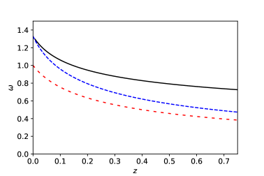
Figure 1: Comparison of the effective excluded volume suppression measures $\omega_{St}$ (solid curve) and $\omega_{Alt}$ (long dashed curve) for the set of parameters given by Eq. (27) (also shown in the legend). For a comparison $\omega_{Alt}$ (short dashed curve) for $A=B=0.5$ is also shown.

In order to compare the obtained alternative ISCT EoS (22) and (23) with the standard one, we consider the one-component case, i.e. one sort of particles. In this case the statistical averaged of the $n$-th power of hard-core radii is equal to the $R_{1}^{n}$ and the quantity $Q$ from Eq. (24) acquires a simple form $Q=\frac{3(A+B)}{R_{1}}$. Let us introduce the following measure of excluded volume suppression $\omega_{St}$ for the standard ISCT EoS formulation and $\omega_{Alt}$ for the alternative one

$${\omega_{St}\equiv\frac{S_{1}\Sigma}{3V_{1}p}+\frac{C_{1}K}{3V_{1}p}}\qquad{\rm and}\qquad\omega_{Alt}\equiv A\frac{S_{1}\xi_{1}}{3V_{1}}+B\frac{C_{1}\xi_{2}}{3V_{1}}=\frac{(A+B)}{R_{1}}\xi_{1}.$$ (26)

Evidently both of these measures show how the difference of the effective excluded volume $V_{1}^{eff}$ (16) and the eigenvolume $V_{1}$ of particles depend on system pressure. In Fig. 1 one can see the comparison of $\omega_{St}$ and $\omega_{Alt}$ for the best set of parameters of the system (13)-(15)

$$A=0.57,\quad B=0.76,\quad\alpha=1.07,\quad\beta=3.76,$$ (27)

which exactly reproduces the five virial coefficients [26] of the famous CS EoS [27] of classical hard spheres. Note that the CS EoS works for hard spheres very well up to the packing fractions $\eta\simeq 0.45$ [7] above which in the system of classical hard spheres there exist a phase transition to the solid phase.

As one can see from Fig. 1 for $z\leq 0.2$ the maximal deviation between $\omega_{Alt}$ and $\omega_{St}$ is less than 20%. Since for $z\leq 0.2$ the excluded volume effect is a correction to the ideal gas EoS, then the 20% deviation of correction between them is, indeed, a tiny correction, which is hard to see.

To demonstrate this in a simple way we consider the one-component system in the canonical ensemble, i.e. the pressure of the one-component system with the suppression due $\xi_{L}$ factors from Eq. (25) which has the form

$$p_{can}\equiv\frac{T\rho}{1-\rho\left[V_{1}+S_{1}\xi\right]}=\frac{T\rho}{1-\rho V_{1}\left[1+\frac{3}{1+\frac{V_{1}p_{can}(A+B)}{T}}\right]},$$ (28)

where instead of the suppression factors $\xi_{1}$ we used its approximation $\xi\equiv\frac{R_{1}}{1+\frac{V_{1}p_{can}(A+B)}{T}}$ which, apparently, works well not only at low and hight particle number density $\rho$. This reasonable approximation has an advantage that equation for the pressure $p_{can}$ can be solved explicitly as

$$p_{can}\equiv\frac{T}{2V_{1}(A+B)}\left[\frac{(3+A+B)\eta}{1-\eta}-1+\sqrt{\left(1-\frac{(3+A+B)\eta}{1-\eta}\right)^{2}+4\frac{(A+B)\eta}{1-\eta}}\right],$$ (29)

where the packing fraction is defined as $\eta=V_{1}\rho$.

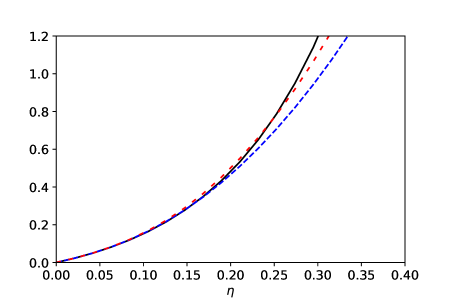
Figure 2: Comparison of the dimensionless pressures $\frac{p_{can}V_{1}}{T}$ for the CS EoS (solid curve) and for the alternative ISCT EoS defined by Eq. (29) for the parameters $A=0.57$ and $B=0.76$ (long dashed curve) and for the parameters $A=0.5$ and $B=0.5$ (short dashed curve).

In Fig. 2 we compare the canonical ensemble pressure (29) (in a dimensionless form) with the famous CS EoS one [27]

$$\frac{p_{can}^{CS}V_{1}}{T}=\frac{\eta(1+\eta+\eta^{2}-\eta^{3})}{(1-\eta)^{3}},$$ (30)

which nowadays is regarded as an exact result for the gaseous phase of classical hard spheres [7, 8]. As one can see from Fig. 2 the pressure (29) for the parameters $A=0.5$ and $B=0.5$ is less accurate for $\eta\in[0.1;0.2]$, than the one for the set with $A=0.57$ and $B=0.76$, but the former one can be used for a wider range of packing fractions, namely for $\eta\leq 0.28$. From Fig. 2 one can see that for packing fractions $\eta\leq 0.15$ the canonical ensemble pressure (29) found for the parameters $A=0.5$ and $B=0.5$ and the one found for $A=0.57$ and $B=0.76$ are hardly distinguishable from each other and from the CS EoS.

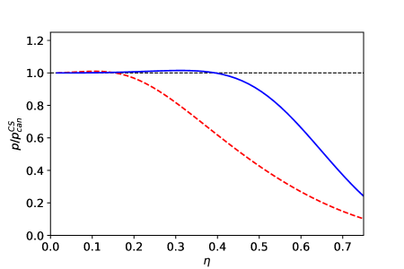
Figure 3: Packing fraction dependence of the ratios $\frac{p_{can}}{p_{can}^{CS}}$ (long dashed curve is found for the parameters $A=0.57$ and $B=0.76$) and $\frac{p_{can}^{G}}{p_{can}^{CS}}$ (solid curve is calculated for $\tilde{A}=0.0215$). For $\eta\leq 0.42$ the maximal relative deviation of the ratio $\frac{p_{can}^{G}}{p_{can}^{CS}}$ from 1 does not exceed 1.5%. The short dashed curve $y=1$ is shown to guide an eye.

Here it is appropriate to discuss the generalization of the canonical ensemble pressure (29) in the spirit of the Guggenheim EoS [48]

$$\frac{p_{can}^{G}V_{1}}{T}\equiv\frac{\eta}{\left(1-\frac{\eta}{4}\left[1+\frac{3}{1+\frac{p_{can}^{G}V_{1}\tilde{A}}{T}}\right]\right)^{4}}\qquad{\rm with}\qquad\tilde{A}\simeq 0.0215.$$ (31)

Evidently, for low packing fractions $\eta<0.1$ the suppression factor is about 1, but at higher packing fractions the presence of suppression factor $\xi^{G}=\frac{1}{1+\frac{p_{can}^{G}V_{1}\tilde{A}}{T}}$ in Eq. (31) allows one to extend the validity range of the alternative ISCT EoS up to $\eta\leq 0.42$ using just a single adjustable parameter $\tilde{A}$. Note that such a generalization automatically reproduces the value of the second and third virial coefficients and, hence, for this case the suppression should be weaken. The latter is seen from the small value of the parameter $\tilde{A}$. As one can see from Fig. 3 the found generalization (31) of the alternative ISCT EoS is able to accurately reproduce the CS EoS with the maximal relative deviation not exceeding 1.5% for $\eta\leq 0.42$. Hence such a generalization can be considered as an additional justification for the nonlinear suppression of interaction suggested recently in Ref. [29, 30].

Now, however, one can clearly see the similarity and difference of the present approach with the density dependent interaction suggested in Ref. [29, 30]. At low densities, both the suppression factor $\xi$ and its generalization $\xi^{G}$ in Eq. (31) behave as a power of packing fraction $\eta$. However, at higher packing fractions one can replace the pressure $p_{can}$ and $p_{can}^{G}$ by the CS one to get an impression about the effect of excluded volume suppression. In the density dependent interaction approach [29] the maximal density is finite and, hence, at high packing fractions interaction does not disappear completely, while in the alternative ISCT EoS the pressure diverges in this limit and the effect of interaction suppression can be stronger, especially for the generalized EoS (31). Moreover, like the nonlinear suppression of interaction suggested in Ref. [29], the generalized EoS (31) clearly demonstrates that higher degree of suppression allows one to correctly reproduce the asymptotic behavior of hard-core repulsion.

The success of the generalized EoS (31) for the one-component system motivates us to generalize the alternative ISCT EoS (22), (23) in a similar way

$$p^{new}=T\sum\limits_{k=1}^{N}\phi_{k}\exp\left[\frac{\mu_{k}}{T}-\frac{p^{new}}{T}(V_{k}+A_{k}S_{k}\xi_{1}+B_{k}C_{k}\xi_{2})\right],\quad{\rm where}$$ (32)

$$\xi_{L}\equiv\frac{\langle{R^{L}}\rangle}{\left[1+\gamma_{1}\frac{p^{new}\langle{V}\rangle}{T}\left[1+\xi_{1}\left(\frac{\langle{A\cdot S}\rangle}{\langle{V}\rangle}+\frac{\langle{B\cdot C}\rangle\langle{S}\rangle}{\langle{V}\rangle\langle{C}\rangle}\right)\right]\right]^{\gamma_{2}}},\quad{\rm for}\quad L=1,2,$$ (33)

where in addition to the global adjustable parameters $\gamma_{1}$ and $\gamma_{2}$ we introduced the parameters $A_{k}$ and $B_{k}$ for the $k$-th sort of particles. As it is argued in Refs. [25, 26] an introduction of the individual parameters $A_{k}$ and $B_{k}$ modifying the eigensurface and eigenperimeter of the standard ISCT EoS may allow one to consider the hard-core repulsion of non-spherical form or even to include the attraction between the constituents. Apparently, the same arguments should be valid for the alternative ISCT EoS.

Another important application of the method developed here is an alternative ISCT EoS for quantum particles with the hard-core repulsion. Applying the method presented in Appendix A to the quantum GCPF of the model M2 from Ref. [25] one can straightforwardly obtain the quantum analog of alternative ISCT EoS (22), (23) from Eqs. (27) and (28) of Ref. [25]. Then generalizing it in the spirit of the system (32), (33) one finds

$$p^{q}=T\sum\limits_{j=1}^{N}g_{j}\int\limits_{M_{j}^{Th}}^{\infty}\frac{dm}{N_{j}(M_{j}^{Th})}\frac{\Gamma_{j}}{(m-m_{j})^{2}+\Gamma^{2}_{j}/4}\times\int\frac{a_{j}d^{3}k}{(2\pi\hbar)^{3}}\ln\left[1+\frac{\exp\left[\frac{\nu_{j}-e(k,m)}{T}\right]}{a_{j}}\right],~{}{\rm with}\qquad~{}$$ (36)

$$\nu_{j}\equiv\mu_{j}-\left[V_{j}+A_{j}S_{j}\xi_{1}+B_{j}C_{j}\xi_{2}\right]p^{q}\,,\quad{\rm and}$$

$$\xi_{L}\equiv\frac{\langle{R^{L}}\rangle}{\left[1+\gamma_{1}\frac{p^{q}\langle{V}\rangle}{T}\left[1+\xi_{1}\left(\frac{\langle{A\cdot S}\rangle}{\langle{V}\rangle}+\frac{\langle{B\cdot C}\rangle\langle{S}\rangle}{\langle{V}\rangle\langle{C}\rangle}\right)\right]\right]^{\gamma_{2}}},\quad{\rm for}\quad L=1,2\,.$$

Here the effective chemical potential of $j$-th sort of particles is $\nu_{j}$, while $e(k,m)=\sqrt{m^{2}+k^{2}}$ denotes the energy of such particles with momentum $\vec{k}$ and mass $m$ over which there is an integration with the Breit-Wigner weight. Note that the expression for normalization factor $N_{j}(M_{j}^{Th})$ coincides with Eq. (10) and $M_{j}^{Th}$, as before, is the decay threshold mass of the $j$-th hadronic resonance which has the full width $\Gamma_{j}$ in the vacuum.

The parameter $a_{j}=+1$ ($a_{j}=-1$) corresponds to the Fermi-Dirac (Bose-Einstein) statistics. One can readily check that in the limit $a_{j}\rightarrow\infty$ Eq. (36) automatically recovers the result (32) for the Boltzmann statistics. The other notations are the same as for the Boltzmann statistics case considered above.

The coefficients $\gamma_{1}$, $\gamma_{2}$, $\{A_{k}\}$ and $\{B_{k}\}$ which are used in the systems (32), (33) and (36)-(36) can be found either from the comparison with the multi-component version of the CS EoS, i.e. the MCSL EoS [28], or from the analysis of the molecular dynamics results which can provide us with a few virial coefficients of multicomponent mixtures. After these coefficients for the classical particles are found they can be used in the quantum version of alternative ISCT EoS. The successful normalization of the standard ISCT EoS to various systems made in Ref. [26] and the example of canonical pressure $p^{G}_{can}$ (31) compared above with the CS EoS can be considered as a perfect warranty that the coefficients $\gamma_{1}$, $\gamma_{2}$, $\{A_{k}\}$ and $\{B_{k}\}$ of the alternative ISCT EoS (32), (33) can provide us with a very accurate description not only of the hard spheres with the multicomponent hard-core repulsion, but also of more complicated interaction between the particles. This, however, is not a trivial numerical task which require a separate study.

4 Conclusions and perspectives

In this work we developed a novel approach to analyze the excluded volume of the multicomponent mixtures of classical hard spheres. Using the Laplace-Fourier technique [44, 45], it was possible to evaluate the grand canonical partition function for the excluded volume which is quadratic in the occupational number of particles under the plausible approximations. To our best knowledge for the arbitrary number of different sorts of hard spheres this is done for the first time.

As a result, the alternative formulation of the ISCT EoS has not an exponential, but the power-like suppression of the induced surface and curvature tension coefficients. Such formulation has some advantages over the standard ISCT EoS formulation. In particular, here it is further generalized with the help of the Guggenheim trick used to obtain his famous EoS [48]. For the one-component case it is shown that the generalized ISCT EoS with a single adjustable parameter is able to reproduce the Carnahan-Starling EoS for the Boltzmann hard spheres with rather good accuracy up to packing fractions $\eta\simeq 0.42$. In the same way we obtain the generalized ISCT EoS for the mixture of quantum particles with the hard-core repulsion.

It is necessary to stress that the hard-core repulsion was considered here because it is the simplest interaction which, nevertheless, correctly reflects the properties of matter at high pressures. It is clear that one can take into account the attractive interaction using the same approach and obtain the power-like suppression. Therefore, the present approach is rather general and, hence, it can be applied not only to develop the realistic EoS for the dense mixtures of hadrons, nuclei and quark-gluon plasma bags and the one for neutron matter with a sizable fraction of hyperons, but to resolve some old problems of dense quantum systems. For example, the classical hard spheres exhibit a deposition phase transition at packing fractions $\eta>0.45$ [7, 8], but to our best knowledge a similar problem for quantum particles is not solved yet. Moreover, recently it was shown [49] that Bose-Einstein condensation of non-relativistic particles with the hard-core repulsion a la VdW is a deposition phase transition similar to the system of classical hard-spheres which belongs to the class of exactly solvable models of nuclear liquid-gas phase transitions discusses in Ref. [2]. However, for an ultimate analysis of this problem one needs a more realistic EoS which is valid at packing fractions $\eta>0.45$.

Moreover, one could apply the Laplace-Fourier technique to the excluded volume of the multi-component mixtures in order to completely abandon the approximative treatment of the mean hard-core radius and the mean square of hard-core radius in Eqs. (18). However, the resulting grand canonical partition function cannot be evaluated using the methods of the present work and, hence, this complicated mathematical task is reserved for the future exploration. It should be also mentioned that after some modifications the present approach can be used not only in the thermodynamic limit, but for the finite volumes of the system, although this task requires a separate analysis.

Acknowledgements. The author thanks Boris Grinyuk, Oleksii Ivanytskyi, Pavlo Panasiuk, Oleksandr Vitiuk and Nazar Yakovenko for fruitful discussions. The author is thankful to Nazar Yakovenko for verifying his calculations and for the help in improving the figures. This work was supported by the National Academy of Sciences of Ukraine under the Project No 0118U003197. The author is grateful to the COST Action CA15213 “THOR“ for supporting his networking.

5 Appendix A: Laplace-Fourier Transform Method

In this Appendix we evaluate the GCPF (19) with the total excluded volume of particles (20) using the Laplace-Fourier transform technique suggested in Refs. [44, 45]. Our first step is to get rid of the nonlinear dependence of $\overline{V}_{excl}$ on $N_{k}$ and to equivalently make it linear in $N_{k}$. For this purpose, prior to the Laplace transform of the GCPF (19) we will introduce in it the new variables $\xi_{1}$ and $\xi_{2}$ and use the following identity suggested in Refs. [44, 45]

$$G(x_{1},x_{2}) \equiv \int\limits_{-\infty}^{+\infty}d\xi_{1}\,\delta(\xi_{1}-x_{1})\int\limits_{-\infty}^{+\infty}d\xi_{2}\,\delta(\xi_{2}-x_{2})G(\xi_{1},\xi_{2})=$$ (A.1)

$$= \int\limits_{-\infty}^{+\infty}d\xi_{1}\,\int\limits_{-\infty}^{+\infty}\frac{d\eta_{1}}{2\pi}\,\int\limits_{-\infty}^{+\infty}d\xi_{2}\,\int\limits_{-\infty}^{+\infty}\frac{d\eta_{2}}{2\pi}\,e^{i\eta_{1}(\xi_{1}-x_{1})}\,e^{i\eta_{2}(\xi_{2}-x_{2})}\,G(\xi_{1},\xi_{2})\,,$$ (A.2)

where Eq. (A.2) is obtained from Eq. (A.1) with the help of the Fourier representation of the Dirac $\delta$-function.

However, a word of caution should be said here. Since we are dealing with the products of generalized functions, it is necessary to define them very carefully before taking the thermodynamic limit $V$. Hence we will apply the identity (A.2) in the meaning of principal value of each $\eta$-integral

$$G(x_{1},x_{2}) = \int\limits_{-\infty}^{+\infty}d\xi_{1}\,\int\limits_{-\infty}^{+\infty}d\xi_{2}\,\int\limits_{-{\cal A}_{1}}^{+{\cal A}_{1}}\frac{d\eta_{1}}{2\pi}\,\int\limits_{-{\cal A}_{2}}^{+{\cal A}_{2}}\frac{d\eta_{2}}{2\pi}\,e^{i\eta_{1}(\xi_{1}-x_{1})}\,e^{i\eta_{2}(\xi_{2}-x_{2})}\,G(\xi_{1},\xi_{2})\,.$$ (A.3)

Moreover, after evaluation the GCPF (19) for large, but finite values of parameters ${\cal A}_{1}$ and ${\cal A}_{2}$, we will find the limits ${\cal A}_{1}\rightarrow+\infty$ and ${\cal A}_{2}\rightarrow+\infty$ before taking the thermodynamic limit $V\rightarrow\infty$.

Next for the identity (A.3) we define the variables $x_{1}$ and $x_{2}$ as

$$x_{1}=\sum\limits_{l}N_{l}R_{l}\biggl{/}\langle N\rangle,\qquad x_{2}=\sum\limits_{l}N_{l}R_{l}^{2}\biggl{/}\langle N\rangle.$$ (A.4)

Before making the Laplace transform of the GCPF (19) it is necessary to note that the major task of this Appendix is to obtain an explicit expression for such a partition as the function of two independent parameters, namely the system volume $V$ and the mean multiplicity of all particles $\langle N\rangle$. Therefore, to reach this goal we will consider the quantity $\langle N\rangle$ as large, but the volume independent parameter. The point is that we would like to exactly make all summations in the system (18)-(20) and get its exact representation in the thermodynamic limit while keeping the quantity $\langle N\rangle$ as an independent parameter. Once the functional dependence of the GCPF (19) on the variables $V$ and $\langle N\rangle$ gets clear, we will easily find the thermodynamic limit using the volume dependence of $\langle N\rangle$. Note, however, that the volume dependence of the quantity $\langle N\rangle$ can be, in principle, taking into account directly by adding the $\xi_{3}$ and $\eta_{3}$ integrals in the identities (A.2) and (A.3), but this will produce unnecessary technical complications of the present work. Therefore, we will not introduce the additional variables $\xi_{3}$ and $\eta_{3}$ and consider $\langle N\rangle$ as a volume independent parameter till the analysis of the thermodynamic limit.

Under these assumptions with the help of the identity (A.3) we represent the GCPF (19) as

$$Z_{GCE}(T,\left\{\mu_{k}\right\},V,\langle N\rangle)\equiv\int\limits_{-\infty}^{+\infty}d\xi_{1}\,\int\limits_{-\infty}^{+\infty}d\xi_{2}\,\int\limits_{-{\cal A}_{1}}^{+{\cal A}_{1}}\frac{d\eta_{1}}{2\pi}\,\int\limits_{-{\cal A}_{2}}^{+{\cal A}_{2}}\frac{d\eta_{2}}{2\pi}\,\exp\left[i\eta_{1}\xi_{1}+i\eta_{2}\xi_{2}\right]\times\,$$

$$\times\sum\limits_{\left\{{N_{k}}\right\}}^{\infty}\left[\prod\limits_{k=1}^{N}\frac{\left(\phi_{k}\exp\left[\frac{\mu_{k}}{T}-i\eta_{1}\frac{R_{k}}{\langle N\rangle}-i\eta_{2}\frac{R_{k}^{2}}{\langle N\rangle}\right]\left[V-\overline{V}_{excl}(\xi_{1},\xi_{2})\right]\right)^{N_{k}}}{N_{k}!}\right]\theta(V-\overline{V}_{excl}(\xi_{1},\xi_{2})),$$ (A.5)

where the total excluded volume now depends on the variables $\xi_{1}$ and $\xi_{2}$ as

$$\overline{V}_{excl}(\xi_{1},\xi_{2})=\sum\limits_{k=1}^{N}N_{k}V_{k}+A\cdot\xi_{1}\sum\limits_{k=1}^{N}N_{k}S_{k}+B\cdot\xi_{2}\sum\limits_{k=1}^{N}N_{k}C_{k}.$$ (A.6)

Now we can make the Laplace transform of the GCPF (5) with respect to system volume while treating $\langle N\rangle$ as a parameter. The corresponding isobaric partition can be written as

$${\cal Z}(T,\left\{\mu_{k}\right\},\lambda,\langle N\rangle)\equiv\int\limits_{0}^{+\infty}dV\,e^{-\lambda V}Z_{GCE}(T,\left\{\mu_{k}\right\},V,\langle N\rangle)=$$ (A.7)

$$=\int\limits_{0}^{+\infty}dV\,\int\limits_{-\infty}^{+\infty}d\xi_{1}\,\int\limits_{-\infty}^{+\infty}d\xi_{2}\,\int\limits_{-{\cal A}_{1}}^{+{\cal A}_{1}}\frac{d\eta_{1}}{2\pi}\,\int\limits_{-{\cal A}_{2}}^{+{\cal A}_{2}}\frac{d\eta_{2}}{2\pi}\,\exp\left[i\eta_{1}\xi_{1}+i\eta_{2}\xi_{2}-\lambda V\right]\times\,$$

$$\times\sum\limits_{\left\{{N_{k}}\right\}}^{\infty}\left[\prod\limits_{k=1}^{N}\frac{\left(\phi_{k}\exp\left[\frac{\mu_{k}}{T}-i\eta_{1}\frac{R_{k}}{\langle N\rangle}-i\eta_{2}\frac{R_{k}^{2}}{\langle N\rangle}\right]\left[V-\overline{V}_{excl}(\xi_{1},\xi_{2})\right]\right)^{N_{k}}}{N_{k}!}\right]\theta(V-\overline{V}_{excl}(\xi_{1},\xi_{2})).\qquad$$ (A.8)

Next we employ the usual trick (for an appropriate review see [2]) to evaluate the summations in Eq. (A.8) and to calculate the integral with respect to $V$, namely we change the order of integrals moving the $\int d\lambda$ to the right position and then we change the variable from $V$ to $\tilde{V}=V-\overline{V}_{excl}(\xi_{1},\xi_{2})$. This change of variables allows one to get rid of the $\Theta$-function constraint. Moving the terms of $\overline{V}_{excl}(\xi_{1},\xi_{2})$ containing the particle multiplicities $N_{k}$ to the appropriate places, after the described change of variables one finds

$${\cal Z}(T,\left\{\mu_{k}\right\},\lambda,\langle N\rangle)=\int\limits_{-\infty}^{+\infty}d\xi_{1}\,\int\limits_{-\infty}^{+\infty}d\xi_{2}\,\int\limits_{-{\cal A}_{1}}^{+{\cal A}_{1}}\frac{d\eta_{1}}{2\pi}\,\int\limits_{-{\cal A}_{2}}^{+{\cal A}_{2}}\frac{d\eta_{2}}{2\pi}\,\int\limits_{0}^{+\infty}d\tilde{V}\,\exp\left[i\eta_{1}\xi_{1}+i\eta_{2}\xi_{2}-\lambda\tilde{V}\right]\times\,$$

$$\times\sum\limits_{\left\{{N_{k}}\right\}}^{\infty}\left[\prod\limits_{k=1}^{N}\frac{\left(\phi_{k}\exp\left[\frac{\mu_{k}}{T}-i\eta_{1}\frac{R_{k}}{\langle N\rangle}-i\eta_{2}\frac{R_{k}^{2}}{\langle N\rangle}-\lambda(V_{k}+AS_{k}\xi_{1}+BC_{k}\xi_{2})\right]\tilde{V}\right)^{N_{k}}}{N_{k}!}\right].\quad$$ (A.9)

Now the summations over $N_{k}$ and product over $k$ can be made exactly, resulting in

$${\cal Z}(T,\left\{\mu_{k}\right\},\lambda,\langle N\rangle)=\int\limits_{-\infty}^{+\infty}d\xi_{1}\,\int\limits_{-\infty}^{+\infty}d\xi_{2}\,\int\limits_{-{\cal A}_{1}}^{+{\cal A}_{1}}\frac{d\eta_{1}}{2\pi}\,\int\limits_{-{\cal A}_{2}}^{+{\cal A}_{2}}\frac{d\eta_{2}}{2\pi}\,\int\limits_{0}^{+\infty}d\tilde{V}\,\exp\left[i\eta_{1}\xi_{1}+i\eta_{2}\xi_{2}\right]\times\,$$ (A.11)

$$\times\exp\left[\tilde{V}\sum\limits_{k=1}^{N}\phi_{k}\exp\left[f_{k}(\lambda,\{\eta_{j}\})\right]-\lambda\tilde{V}\right],\quad$$

$${\rm where}~{}~{}f_{k}(\lambda,\{\eta_{j}\})\equiv\frac{\mu_{k}}{T}-i\eta_{1}\frac{R_{k}}{\langle N\rangle}-i\eta_{2}\frac{R_{k}^{2}}{\langle N\rangle}-\lambda(V_{k}+AS_{k}\xi_{1}+BC_{k}\xi_{2}).$$

Apparently, the integral with respect to the variable $\tilde{V}$ can be calculated easily and the isobaric partition (A.7) acquires the form

$${\cal Z}(T,\left\{\mu_{k}\right\},\lambda,\langle N\rangle)=\int\limits_{-\infty}^{+\infty}d\xi_{1}\,\int\limits_{-\infty}^{+\infty}d\xi_{2}\,\int\limits_{-{\cal A}_{1}}^{+{\cal A}_{1}}\frac{d\eta_{1}}{2\pi}\,\int\limits_{-{\cal A}_{2}}^{+{\cal A}_{2}}\frac{d\eta_{2}}{2\pi}\,\,\exp\left[i\eta_{1}\xi_{1}+i\eta_{2}\xi_{2}\right]\left[\lambda-\cal{F(\lambda)}\right]^{-1},\qquad$$ (A.12)

$${\rm where}~{}~{}{\cal{F(\lambda,\{\eta_{j}\})}}\equiv\sum\limits_{k=1}^{N}\phi_{k}\exp\left[f_{k}(\lambda,\{\eta_{j}\})\right].$$ (A.13)

Although all summations and the product of the original GCPF (5) we calculated exactly the evaluation of the inverse Laplace transform of the isobaric partition (A.12) will be made under a plausible approximation in order to simplify the presentation of the major result of the present approach. Since the functional $\lambda$-dependence of the isobaric partition (A.12) is similar to the standard case [2], then we conclude that in the thermodynamic limit the leading singularity (or the rightmost singularity) of the partition (A.12) is the simple pole. The main difference, however, from the standard case is that this pole $\lambda_{c}=\lambda_{0}+i\delta_{1}\lambda$ is not the real one, but a complex one.

Now we recall the fact that the variables $\eta_{1}\in[-{\cal A}_{1};+{\cal A}_{1}]$ and $\eta_{2}\in[-{\cal A}_{2};+{\cal A}_{2}]$ are restricted from above. Therefore, we can choose so large values of $\langle N\rangle$, i.e. very large volume of the system, that the quantities

$$|\eta_{1}|\frac{R_{k}}{\langle N\rangle}\ll 1,\qquad|\eta_{2}|\frac{R_{k}^{2}}{\langle N\rangle}\ll 1,$$ (A.14)

can be made as small as necessary. Hence, one can make an expansion of the function ${\cal F}(\lambda_{c})$ as follows

$${\cal F}(\lambda_{c},\{\eta_{j}\})\simeq{\cal F}(\lambda_{c},\{0\})-\Phi_{1}(\lambda_{c})i\frac{\eta_{1}}{\langle N\rangle}-\Phi_{2}(\lambda_{c})i\frac{\eta_{2}}{\langle N\rangle},$$ (A.15)

$${\rm where}~{}~{}\Phi_{L}(\lambda_{c})\equiv T\sum\limits_{k=1}^{N}\frac{\partial{\cal F}(\lambda_{c},\{0\})}{\partial\mu_{k}}R_{k}^{L}=\sum\limits_{k=1}^{N}R_{k}^{L}\phi_{k}\exp\left[f_{k}(\lambda_{c},\{0\})\right],\quad{\rm for}\quad L=1,2.\qquad$$ (A.16)

Using this expansion we can find the simple pole of the isobaric partition in the complex $\lambda$-plane.

Due to inequalities (A.14) the terms containing the ratios $\frac{\eta_{1}}{\langle N\rangle}$ and $\frac{\eta_{2}}{\langle N\rangle}$ which are staying on the right hand side of Eq. (A.15) are small corrections to the term ${\cal F}(\lambda_{c},\{0\})$, hence the imaginary part of the pole $\lambda_{c}=\lambda_{0}+i\delta_{1}\lambda$, i.e. $\delta_{1}\lambda$ is also small correction to $\lambda_{0}$. Therefore in solving the equation for $\lambda_{c}$

$$0=\lambda_{c}-{\cal F}(\lambda_{c},\{\eta_{j}\})\simeq\lambda_{0}+i\delta_{1}\lambda-{\cal F}(\lambda_{c},\{0\})+\Phi_{1}(\lambda_{c})i\frac{\eta_{1}}{\langle N\rangle}+\Phi_{2}(\lambda_{c})i\frac{\eta_{2}}{\langle N\rangle},$$ (A.17)

one can safely expand the function ${\cal F}(\lambda_{c},\{0\})$ in the vicinity of the point $\lambda=\lambda_{0}$, but at the same time one can also safely approximate $\Phi_{L}(\lambda_{c})\simeq\Phi_{L}(\lambda_{0})$, since the term $\delta_{1}\lambda$ will generate the higher order corrections which are not considered here (apparently, by a proper choice of $\langle N\rangle$ one can make the higher order corrections negligible). Taking this fact into account one finds the equation for pole $\lambda_{c}$ as

$$0=\lambda_{c}-{\cal F}(\lambda_{c},\{\eta_{j}\})\simeq$$

$$\simeq\lambda_{0}+i\delta_{1}\lambda-{\cal F}(\lambda_{0},\{0\})-\frac{\partial{\cal F}(\lambda_{0},\{0\})}{\partial\lambda_{0}}i\delta_{1}\lambda+\Phi_{1}(\lambda_{0})i\frac{\eta_{1}}{\langle N\rangle}+\Phi_{2}(\lambda_{0})i\frac{\eta_{2}}{\langle N\rangle}~{}~{}\Rightarrow$$ (A.18)

$$\lambda_{0}-{\cal F}(\lambda_{0},\{0\})=0,~{}~{}{\rm and}~{}~{}\delta_{1}\lambda\simeq-\left[\Phi_{1}(\lambda_{0})\frac{\eta_{1}}{\langle N\rangle}+\Phi_{2}(\lambda_{0})\frac{\eta_{2}}{\langle N\rangle}\right]\left[1-\frac{\partial{\cal F}(\lambda_{0},\{0\})}{\partial\lambda_{0}}\right]^{-1}.~{}$$ (A.19)

These expressions above define the real part of $\lambda_{c}$ as $\lambda_{0}=Re(\lambda_{c})$ and its imaginary part as $\delta_{1}\lambda=Im(\lambda_{c})$. With their help one can easily the residue at the pole $\lambda=\lambda_{c}$. Choosing $\lambda=\lambda_{R}+i\delta_{1}\lambda$ with $\lambda_{R}\rightarrow\lambda_{0}$, one can write the right hand side Eq. (A.17) as

$$\lambda_{R}+i\delta_{1}\lambda-{\cal F}(\lambda_{R}+i\delta_{1}\lambda,\{0\})+\Phi_{1}(\lambda_{0})i\frac{\eta_{1}}{\langle N\rangle}+\Phi_{2}(\lambda_{0})i\frac{\eta_{2}}{\langle N\rangle}\rightarrow$$ (A.20)

$$\rightarrow\lambda_{R}+i\delta_{1}\lambda-{\cal F}(\lambda_{0},\{0\})-\frac{\partial{\cal F}(\lambda_{0},\{0\})}{\partial\lambda_{0}}[\lambda_{R}+i\delta_{1}\lambda-\lambda_{0}]+\Phi_{1}(\lambda_{0})i\frac{\eta_{1}}{\langle N\rangle}+\Phi_{2}(\lambda_{0})i\frac{\eta_{2}}{\langle N\rangle},\qquad$$ (A.21)

where in Eq (A.20) we expanded the function ${\cal F}(\lambda,\{0\})$ at the point $\lambda=\lambda_{0}$. Applying the expressions (A.19) to Eq. (A.21), one finds the residue at the pole $\lambda_{c}$ as

$$Res\left(\left[\lambda-{\cal F}(\lambda,\{0\})+\Phi_{1}(\lambda_{0})i\frac{\eta_{1}}{\langle N\rangle}+\Phi_{2}(\lambda_{0})i\frac{\eta_{2}}{\langle N\rangle}\right]^{-1}\right)\Biggl{|}_{\lambda_{c}}=\left[1-\frac{\partial{\cal F}(\lambda_{0},\{0\})}{\partial\lambda_{0}}\right]^{-1}.$$ (A.22)

With the help of last result one can perform the inverse Laplace transform of the isobaric partition (A.12). Indeed, choosing the integration contour in the complex $\lambda$-plane to be on the right hand side of $\lambda_{c}$, i.e. with $\chi>\lambda_{0}$, one can make the inverse Laplace transform with respect to $\lambda$ in the following set of steps: first, we write the definition

$$Z_{GCE}(T,\left\{\mu_{k}\right\},V,\langle N\rangle)=\int\limits_{\chi-i\infty}^{\chi+i\infty}\frac{d\lambda}{2\pi i}\,e^{+\lambda V}{\cal Z}(T,\left\{\mu_{k}\right\},\lambda,\langle N\rangle)\simeq$$ (A.23)

$$\simeq\int\limits_{\chi-i\infty}^{\chi+i\infty}\frac{d\lambda}{2\pi i}\,e^{+\lambda V}\int\limits_{-\infty}^{+\infty}d\xi_{1}\,\int\limits_{-\infty}^{+\infty}d\xi_{2}\,\int\limits_{-{\cal A}_{1}}^{+{\cal A}_{1}}\frac{d\eta_{1}}{2\pi}\,\int\limits_{-{\cal A}_{2}}^{+{\cal A}_{2}}\frac{d\eta_{2}}{2\pi}\,{\exp\left[i\eta_{1}\xi_{1}+i\eta_{2}\xi_{2}+\lambda V\right]}\times$$

$$\times\left[\lambda-{\cal F}(\lambda,\{0\})+\Phi_{1}(\lambda_{0})i\frac{\eta_{1}}{\langle N\rangle}+\Phi_{2}(\lambda_{0})i\frac{\eta_{2}}{\langle N\rangle}\right]^{-1}\,,$$ (A.24)

next we change the order of integration and move the integral with respect to $\lambda$ to the rightmost position, apply the Cauchy theorem on residues and get

$$Z_{GCE}(T,\left\{\mu_{k}\right\},V,\langle N\rangle) \simeq\int\limits_{-\infty}^{+\infty}d\xi_{1}\,\int\limits_{-\infty}^{+\infty}d\xi_{2}\,\int\limits_{-{\cal A}_{1}}^{+{\cal A}_{1}}\frac{d\eta_{1}}{2\pi}\,\int\limits_{-{\cal A}_{2}}^{+{\cal A}_{2}}\frac{d\eta_{2}}{2\pi}\,\frac{\exp\left[i\eta_{1}\xi_{1}+i\eta_{2}\xi_{2}+\lambda_{c}V\right]}{\left[1-\frac{\partial{\cal F}(\lambda_{0},\{0\})}{\partial\lambda_{0}}\right]}=\qquad$$ (A.26)

$$=\int\limits_{-\infty}^{+\infty}d\xi_{1}\,\int\limits_{-\infty}^{+\infty}d\xi_{2}\,\int\limits_{-{\cal A}_{1}}^{+{\cal A}_{1}}\frac{d\eta_{1}}{2\pi}\,\int\limits_{-{\cal A}_{2}}^{+{\cal A}_{2}}\frac{d\eta_{2}}{2\pi}\,\frac{\exp\left[i\eta_{1}\xi_{1}+i\eta_{2}\xi_{2}+\lambda_{0}V\right]}{\left[1-\frac{\partial{\cal F}(\lambda_{0},\{0\})}{\partial\lambda_{0}}\right]}\times$$

$$\times\exp\left[-iV\left[\Phi_{1}(\lambda_{0})\frac{\eta_{1}}{\langle N\rangle}+\Phi_{2}(\lambda_{0})\frac{\eta_{2}}{\langle N\rangle}\right]\left[1-\frac{\partial{\cal F}(\lambda_{0},\{0\})}{\partial\lambda_{0}}\right]^{-1}\right],~{}$$

where in the last step of evaluation we substituted the expressions (A.19) for $\lambda_{c}$ into Eq. (A.26).

Since $\lambda_{0}$ is related to the system pressure as $\lambda_{0}=\frac{p}{T}$ (see Refs. [2, 44]), for large volume $V$ one can write $\frac{V}{\langle N\rangle}=\frac{T}{p}=\lambda_{0}^{-1}$. Applying this relation to Eq. (A.26), one can now safely find the limits ${\cal A}_{1}\rightarrow+\infty$ and ${\cal A}_{2}\rightarrow+\infty$ in Eq. (A.26), integrate over $\eta_{1}$ and $\eta_{2}$ and obtain

$$Z_{GCE}(T,\left\{\mu_{k}\right\},V,\langle N\rangle)\simeq\int\limits_{-\infty}^{+\infty}d\xi_{1}\,\int\limits_{-\infty}^{+\infty}d\xi_{2}\,\frac{\exp\left[\lambda_{0}V\right]}{\left[1-\frac{\partial{\cal F}(\lambda_{0},\{0\})}{\partial\lambda_{0}}\right]}\times$$

$$\times\,\delta\left(\xi_{1}-\frac{\Phi_{1}(\lambda_{0})}{\lambda_{0}\left[1-\frac{\partial{\cal F}(\lambda_{0},\{0\})}{\partial\lambda_{0}}\right]}\right)\delta\left(\xi_{2}-\frac{\Phi_{2}(\lambda_{0})}{\lambda_{0}\left[1-\frac{\partial{\cal F}(\lambda_{0},\{0\})}{\partial\lambda_{0}}\right]}\right).$$ (A.27)

Apparently, the integrations over $\xi_{1}$ and $\xi_{2}$ variables are trivial and, finally, the original GCPF (5) can be now written as

$$Z_{GCE}(T,\left\{\mu_{k}\right\},V,\langle N\rangle)\simeq\frac{\exp\left[\lambda_{0}V\right]}{\left[1-\frac{\partial{\cal F}(\lambda_{0},\{0\})}{\partial\lambda_{0}}\right]}\Biggl{|}_{\xi_{1}=\frac{\Phi_{1}(\lambda_{0})}{\lambda_{0}\left[1-\frac{\partial{\cal F}(\lambda_{0},\{0\})}{\partial\lambda_{0}}\right]};~{}\xi_{2}=\frac{\Phi_{2}(\lambda_{0})}{\lambda_{0}\left[1-\frac{\partial{\cal F}(\lambda_{0},\{0\})}{\partial\lambda_{0}}\right]}}.$$ (A.28)

One can readily check that, if in Eq. (A.28) one assumes $R_{k}=0$ and $R_{k}^{2}=0$ in functions $\Phi_{L}(\lambda_{0})$ and ${\cal F}(\lambda_{0},\{0\})$ while keeping $V_{k}\neq 0$, the obtained result coincides with the usual GCPF of particles with the hard-core interaction in the limit of eigenvolume approximation [2].

The final system of equations for the pressure $p=T\lambda_{0}$ and for the quantities $\xi_{1}$ and $\xi_{2}$ can be written as

$$p=T\sum\limits_{k=1}^{N}\phi_{k}\exp\left[\frac{\mu_{k}}{T}-\frac{p}{T}(V_{k}+AS_{k}\xi_{1}+BC_{k}\xi_{2})\right],\quad{\rm where}$$ (A.29)

$$\xi_{L}=\frac{\Phi_{L}\left(\frac{p}{T}\right)}{p\left[1-\frac{\partial{\cal F}(\lambda_{0},\{0\})}{\partial\lambda_{0}}\right]},\quad{\rm for}\quad L=1,2.$$ (A.30)

A detailed analysis of the derived EoS (A.29), (A.30) is made in Section 3.

6 Appendix B: Expressions for the particle number density

In this Appendix we summarize the expressions for the particle number density of the systems (32), (33) and (36)-(36). First we consider the system (32), (33) for the Boltzmann particles. Introducing the partial pressure $p_{k}^{new}$, the partial coefficients for the surface tension $\Sigma_{k}^{new}$ and the partial coefficients for the curvature tension $K_{k}^{new}$ of the $k$-th sort of particles, one can rewrite the system (32), (33) as

$$p^{new}\equiv\sum\limits_{k=1}^{N}p_{k}^{new}=T\sum\limits_{k=1}^{N}\phi_{k}\exp\left[\frac{\mu_{k}-V_{k}p^{new}+A_{k}S_{k}\Sigma^{new}+B_{k}C_{k}K^{new}}{T}\right],\quad$$ (B.1)

$$\Sigma^{new}\equiv\sum\limits_{k=1}^{N}\Sigma_{k}^{new}=\frac{1}{G^{\gamma_{2}}}\sum\limits_{k=1}^{N}R_{k}p_{k}^{new},\quad$$ (B.2)

$$K^{new}\equiv\sum\limits_{k=1}^{N}K_{k}^{new}=\frac{1}{G^{\gamma_{2}}}\sum\limits_{k=1}^{N}R_{k}^{2}p_{k}^{new},\quad$$ (B.3)

$$G\equiv 1+\gamma_{1}\sum\limits_{j=1}^{N}F_{j}\equiv 1+\gamma_{1}\sum\limits_{j=1}^{N}\frac{(V_{j}p^{new}+A_{j}S_{j}\Sigma^{new}+B_{j}C_{j}K^{new})}{T}.$$ (B.4)

Differentiating Eqs. (B.1)-(B.3) of this Appendix with respect to the chemical potential $\mu_{k}$, one can find the particle number density of the $k$-th sort of particles $\rho_{k}=\frac{\partial p^{new}}{\partial\mu_{k}}$ and the derivatives $\frac{\partial\Sigma^{new}}{\partial\mu_{k}}$ and $\frac{\partial K^{new}}{\partial\mu_{k}}$. Solving the system of three equations for these quantities, one can find the particle number density of the $k$-th sort of particles $\rho_{k}$ as

$$\rho_{k}=\frac{1}{T}\frac{(ej-fh)B^{(1)}_{k}-(bj-ch)B^{(2)}_{k}+(bf-ce)B^{(3)}_{k}}{a(ej-fh)-d(bj-ch)+g(bf-ce)}\,,$$ (B.5)

where the coefficients $a,b,c,d,e,f,g,h$, $j$, $B^{(1)}_{k}$, $B^{(2)}_{k}$ and $B^{(3)}_{k}$ are given by

$$a=1+\sum_{k}V_{k}\frac{p_{k}^{new}}{T},\quad\quad b=\sum_{k}A_{k}S_{k}\frac{p_{k}^{new}}{T},\qquad~{}c=\sum_{k}B_{k}C_{k}\frac{p_{k}^{new}}{T},$$ (B.9)

$$d=\sum_{k}V_{k}\frac{B^{(2)}_{k}}{T},\qquad\quad~{}e=1+\sum_{k}A_{k}S_{k}\frac{B^{(2)}_{k}}{T},\quad f=\sum_{k}B_{k}C_{k}\frac{B^{(2)}_{k}}{T},\quad$$

$$g=\sum_{k}V_{k}\frac{B^{(3)}_{k}}{T},\qquad\quad~{}h=\sum_{k}A_{k}S_{k}\frac{B^{(3)}_{k}}{T},\qquad~{}j=1+\sum_{k}B_{k}C_{k}\frac{B^{(3)}_{k}}{T},$$

$$B^{(1)}_{k}=p_{k}^{new},\qquad B^{(2)}_{k}=\Sigma_{k}^{new}-\frac{\gamma_{1}\gamma_{2}\Sigma^{new}}{G}F_{k},\qquad B^{(3)}_{k}=K_{k}^{new}-\frac{\gamma_{1}\gamma_{2}K^{new}}{G}F_{k}.~{}$$

Writing the quantum ISCT EoS (32)-(36) similarly to the system (B.1)-(B.4) of this Appendix

$$p^{q}\equiv T\sum\limits_{j=1}^{N}g_{j}\int\limits_{M_{j}^{Th}}^{\infty}\frac{dm}{N_{j}(M_{j}^{Th})}\frac{\Gamma_{j}}{(m-m_{j})^{2}+\Gamma^{2}_{j}/4}\int\frac{a_{j}d^{3}k}{(2\pi\hbar)^{3}}\ln\left[1+\frac{1}{a_{j}}\exp\left[\frac{\nu_{j}-e(k,m)}{T}\right]\right],\quad$$ (B.10)

$$\Sigma^{q}\equiv\sum\limits_{k=1}^{N}\Sigma_{k}^{q}=\frac{1}{(G_{q})^{\gamma_{2}}}\sum\limits_{k=1}^{N}R_{k}p_{k}^{q},\quad$$ (B.11)

$$K^{q}\equiv\sum\limits_{k=1}^{N}K_{k}^{q}=\frac{1}{(G_{q})^{\gamma_{2}}}\sum\limits_{k=1}^{N}R_{k}^{2}p_{k}^{q},\quad$$ (B.12)

$$G_{q}\equiv 1+\gamma_{1}\sum\limits_{j=1}^{N}\frac{(V_{j}p^{q}+A_{j}S_{j}\Sigma^{q}+B_{j}C_{j}K^{q})}{T},$$ (B.13)

$$\nu_{k}\equiv\mu_{k}-\left[V_{k}p^{q}+A_{k}S_{k}\Sigma^{q}+B_{k}C_{k}K^{q}\right]\,,$$ (B.14)

one can easily show that Eq. (B.5) remains valid for the quantum case as well, if one makes the necessary replacements in Eqs. (B.9)-(B.9)

$$\rho_{k}^{q}=\frac{1}{T}\frac{(ej-fh)B^{(q1)}_{k}-(bj-ch)B^{(q2)}_{k}+(bf-ce)B^{(q3)}_{k}}{a(ej-fh)-d(bj-ch)+g(bf-ce)}\,,$$ (B.20)

$$a=1+\sum_{k}V_{k}n_{k}^{q},\quad\quad b=\sum_{k}A_{k}S_{k}n_{k}^{q},\qquad~{}c=\sum_{k}B_{k}C_{k}n_{k}^{q},$$

$$d=\sum_{k}V_{k}\frac{B^{(q2)}_{k}}{T},\qquad\quad~{}e=1+\sum_{k}A_{k}S_{k}\frac{B^{(q2)}_{k}}{T},\quad f=\sum_{k}B_{k}C_{k}\frac{B^{(q2)}_{k}}{T},\quad$$

$$g=\sum_{k}V_{k}\frac{B^{(q3)}_{k}}{T},\qquad\quad~{}h=\sum_{k}A_{k}S_{k}\frac{B^{(q3)}_{k}}{T},\qquad~{}j=1+\sum_{k}B_{k}C_{k}\frac{B^{(q3)}_{k}}{T},$$

$$B^{(q1)}_{k}=Tn_{k}^{q},~{}\quad B^{(2)}_{k}=T\left[\frac{R_{k}n_{k}^{q}}{G_{q}^{\gamma_{2}}}-\frac{\gamma_{1}\gamma_{2}\Sigma^{q}}{G_{q}}H_{k}^{q}\right],\quad B^{(3)}_{k}=T\left[\frac{R_{k}^{2}n_{k}^{q}}{G_{q}^{\gamma_{2}}}-\frac{\gamma_{1}\gamma_{2}K^{q}}{G_{q}}H_{k}^{q}\right],\qquad$$

$$H_{k}^{q}\equiv(V_{k}+A_{k}S_{k}R_{k}+B_{k}C_{k}R_{k}^{2})n_{k}^{q}=V_{k}(1+1.5A_{k}+1.5B_{k})n_{k}^{q},$$

where $n_{k}^{q}$ denotes the particle number density of quantum particles of the $k$-th sort with the effective chemical potential $\nu_{k}$. It can be written explicitly as

$$n_{j}^{q} \equiv \frac{\partial p_{j}^{q}(T,\nu_{j})}{\partial\nu_{j}}=$$ (B.21)

$$= g_{j}\int\limits_{M_{j}^{Th}}^{\infty}\frac{dm}{N_{j}(M_{j}^{Th})}\frac{\Gamma_{j}}{(m-m_{j})^{2}+\Gamma^{2}_{j}/4}\times\int\frac{d^{3}k}{(2\pi\hbar)^{3}}\left[\exp\left[\frac{e(k,m)-\nu_{j}}{T}\right]+\frac{1}{a_{j}}\right]^{-1}.\quad$$

References

References

• [1] K. A. Bugaev, Phys. Rev. C 76, 014903 (2007); arXiv:0703222 [hep-ph] and references therein.
• [2] K. A. Bugaev and P. T. Reuter, Ukr. J. Phys. 52, 489 (2007); [arXiv:1001.4477 [nucl-th]].
• [3] K. A. Bugaev, V. K. Petrov and G. M. Zinovjev, Phys. Rev. C 79, 054913โ€“1-12 (2009).
• [4] A. I. Ivanytskyi and K. A. Bugaev, Ukr. J. Phys. 57, 964 (2012) and references therein.
• [5] A. I. Ivanytskyi, K. A. Bugaev, A. S. Sorin and G. M. Zinovjev, Phys. Rev. E 86, 061107 (2012) and references therein.
• [6] K. A. Bugaev, V. K. Petrov and G. M. Zinovjev, Phys. Atom. Nucl. 76, 341 (2013) and references therein.
• [7] J. P. Hansen and I. R. McDonald, Theory of Simple Fluids (Academic Press, Amsterdam, 2006).
• [8] Theory and Simulation of Hard Sphere Fluids and Related Systems, Lect. Notes Phys. Vol. 753, edited by A. Mulero (Springer-Verlag, Berlin, 2008).
• [9] V. V. Sagun, A. I. Ivanytskyi, K. A. Bugaev and I. N. Mishustin, Nucl. Phys. A 924, 24 (2014).
• [10] K. A. Bugaev et al., Nucl. Phys. A 970, 133 (2018).
• [11] K. A. Bugaev et al., Phys. Part. Nucl. Lett. 15, 210-224 (2018).
• [12] A.ย I.ย Ivanytskyi, K.ย A.ย Bugaev, V.ย V.ย Sagun, L.ย V.ย Bravina and E.ย E.ย Zabrodin, Phys. Rev. C 97, 064905โ€“1-8 (2018).
• [13] V. V. Sagun et al., Eur. Phys. J. A 54, 100 (2018).
• [14] K. A. Bugaev, A. I. Ivanytskyi, V. V. Sagun, E. G. Nikonov and G. M. Zinovjev, Ukr. J. Phys. 63, 863-880 (2018).
• [15] V.ย V.ย Sagun, I.ย Lopes and A.ย I.ย Ivanytskyi, Astrophys. J. 871, 157 (2019).
• [16] V.ย Sagun, G.ย Panotopoulos and I.ย Lopes, Phys. Rev. D 101, 063025 (2020) and references therein.
• [17] K. A. Bugaev et al., J. of Phys. Conf. Series 1390, 012038, p. 1-6 (2019).
• [18] B. E. Grinyuk et al., arXiv:2004.05481v1 [hep-ph] (2020) p. 1-15. (to appear in Int. J. Mod. Phys. A)
• [19] K. A. Bugaev et al., Eur. Phys. J. A 56, 293โ€“1-15 (2020) (doi.org/10.1140/epja/s10050-020-00296-5); arXiv:2005.01555v1 [nucl-th].
• [20] O.ย V.ย Vitiuk et al., arXiv:2007.07376 [hep-ph] (2020) p. 1-12.
• [21] P. Danielewicz, R. Lacey, and W. G. Lynch, Science 298, 1593 (2002).
• [22] M. Albright, J. Kapusta and C. Young, Phys. Rev. C 90, 024915 (2014).
• [23] S. Chatterjee et al., Adv. High Energy Phys. 2015, 349013 (2015).
• [24] A. Andronic, P. Braun-Munzinger, K. Redlich and J. Stachel, J. Phys. Conf. Ser. 779, 012012 (2017).
• [25] K. A. Bugaev, Eur. Phys. J. A 55, 215 (2019).
• [26] N. S. Yakovenko, K. A. Bugaev, L.V. Bravina and E. E. Zabrodin, arXiv:1910.04889 [nucl-th] (2019) p. 1-13 (to appear in EPJ ST)
• [27] N. F. Carnahan and K. E. Starling, J. Chem. Phys. 51, 635 (1969).
• [28] G. A. Mansoori, N. F. Carnahan, K. E. Starling, T. Leland, J. Chem. Phys. 54, 1523, (1971).
• [29] O.ย Lourenรงo, M.ย Dutra, C.ย H.ย Lenzi, M.ย Bhuyan, S.ย K.ย Biswal and B.ย M.ย Santos, arXiv:1908.05114 [nucl-th] (2019) p. 1-11.
• [30] M.ย Dutra, B.ย M.ย Santos and O.ย Lourenรงo, J. Phys. G 47, 035101 (2020).
• [31] M. A. Stephanov, K. Rajagopal and E. V. Shuryak, Phys. Rev. Lett. 81, 4816 (1998).
• [32] G. Zeeb, K. A. Bugaev, P. T. Reuter and H. Stรถcker, Ukr. J. Phys. 53, 279-295 (2008).
• [33] D. R. Oliinychenko, K. A. Bugaev and A. S. Sorin, Ukr. J. Phys. 58, 211-227 (2013).
• [34] K. A. Bugaev, D. R. Oliinychenko, A. S. Sorin and G. M. Zinovjev, Eur. Phys. J. A 49, 30 (2013).
• [35] A. Dillmann, G. E. Meier, J. Chem. Phys. 94, 3872 (1991).
• [36] M. E. Fisher, Physics 3, 255 (1967).
• [37] A. Laaksonen, I. J. Ford, M. Kulmala, Phys. Rev. E 49, 5517 (1994).
• [38] J. Rafelski, Phys. Lett. B 62, 333 (1991).
• [39] J.ย Hรผfner, S.ย P.ย Klevansky, P.ย Zhuang and H.ย Voss, Annals Phys.ย  234, 225 (1994).
• [40] A.ย Wergieluk, D.ย Blaschke, Y.ย L.ย Kalinovsky and A.ย Friesen, Phys.ย Part.ย Nucl.ย Lett.ย  10, 660 (2013).
• [41] D.ย Blaschke, M.ย Buballa, A.ย Dubinin, G.ย Rรถpke and D.ย Zablocki, Annals Phys.ย  348, 228 (2014) and references therein.
• [42] K. A. Bugaev, A. I. Ivanytskyi, D. R. Oliinychenko, E. G. Nikonov, V. V. Sagun and G. M. Zinovjev, Ukr. J. Phys. 60, 181 (2015) and references therein.
• [43] V. I.ย  Kuksa, Phys. Part. Nucl. 45, 998 (2014) (in Russian) and references therein.
• [44] K. A. Bugaev, Acta. Phys. Polon. B 36, 3083-3094 (2005).
• [45] K. A. Bugaev, L. Phair and J. B. Elliott, Phys. Rev. E 72, 047106 (2005).
• [46] J. Rozynek, J. Phys. G 42, 045109 (2015).
• [47] J. Rozynek, Int. J. Mod. Phys. E 27, 1850030 (2018) and references therein.
• [48] E. A. Guggenheim, Mol. Phys. 9, 199 (1965).
• [49] K.ย A.ย Bugaev, O.ย I.ย Ivanytskyi, B.ย E.ย Grinyuk and I.ย P.ย Yakimenko, Ukr. J. Phys. 65, 963-972 (2020); [arXiv:2009.02178 [nucl-th]]