A phase field formulation for dissolution-driven stress corrosion cracking
Abstract
We present a new theoretical and numerical framework for modelling mechanically-assisted corrosion in elastic-plastic solids. Both pitting and stress corrosion cracking (SCC) can be captured, as well as the pit-to-crack transition. Localised corrosion is assumed to be dissolution-driven and a formulation grounded upon the film rupture-dissolution-repassivation mechanism is presented to incorporate the influence of film passivation. The model incorporates, for the first time, the role of mechanical straining as the electrochemical driving force, accelerating corrosion kinetics. The computational complexities associated with tracking the evolving metal-electrolyte interface are resolved by making use of a phase field paradigm, enabling an accurate approximation of complex SCC morphologies. The coupled electro-chemo-mechanical formulation is numerically implemented using the finite element method and an implicit time integration scheme; displacements, phase field order parameter and concentration are the primary variables. Five case studies of particular interest are addressed to showcase the predictive capabilities of the model, revealing an excellent agreement with analytical solutions and experimental measurements. By modelling these paradigmatic 2D and 3D boundary value problems we show that our formulation can capture: (i) the transition from activation-controlled corrosion to diffusion-controlled corrosion, (ii) the sensitivity of interface kinetics to mechanical stresses and strains, (iii) the role of film passivation in reducing corrosion rates, and (iv) the dependence of the stability of the passive film to local strain rates. The influence of these factors in driving the shape change of SCC defects, including the pit-to-crack transition, is a natural outcome of the model, laying the foundations for a mechanistic assessment of engineering materials and structures.
keywords:
Phase field , Finite element method , Stress corrosion cracking , Passive film , Mechanochemistry1 Introduction
The reliability and structural integrity of materials are generally governed by their interaction with the environment and the multi-physics phenomena resulting from those interactions. Stress corrosion cracking (SCC) is one of these phenomena, arguably the most common yet complex failure mechanism of engineering structures and components (Turnbull, 2001). SCC involves the propagation of cracks due to the combined action of mechanical stresses and the environment. It is often facilitated by pre-existing defects, such as corrosion pits, and takes place in a broad range of metallic materials and environments (Raja and Shoji, 2011). However, and despite decades of intensive research, the underlying physical mechanisms governing SCC are still not well understood (Turnbull, 1993; Crane and Gangloff, 2016). A number of mechanistic interpretations have been presented, and models can be classified into two categories. The first one refers to models and mechanisms where crack propagation is driven by the anodic corrosion reaction at the crack tip, including the active path dissolution model (Parkins, 1996) or models grounded on the film rupture-dissolution-repassivation (FRDR) mechanism (Scully, 1975, 1980; Andresen and Ford, 1988). The second category includes models where crack growth is cathodic-driven and associated with the ingress and transport of hydrogen, such as the hydrogen-enhanced decohesion (HEDE) mechanism (Oriani, 1972; Serebrinsky et al., 2004; Kristensen et al., 2020), hydrogen enhanced localized plasticity (HELP) (Sofronis and Birnbaum, 1995) or adsorption-induced dislocation emission (AIDE) (Lynch, 1988). The characteristics of SCC can vary significantly from one material to another, or even between different environments within the same material, hindering a critical evaluation of the different mechanistic interpretations. Moreover, many of these mechanisms are not mutually exclusive and could be acting in concert.
The development of predictive models for SCC is not only hindered by the complexity of the physical picture but also by the challenges associated with encapsulating into a numerical framework the different physics of the problem (diffusion, electrochemistry, mechanics). It is particularly challenging from a mathematical and computational perspective to capture how the metal-electrolyte interface evolves over time. SCC failures typically involve the growth of multiple pits, a pit-to-crack transition stage and the propagation of one or multiple cracks (Larrosa et al., 2018). Capturing the complex morphologies resulting from this three-stage process is not an easy task and typically requires defining moving interfacial boundary conditions and manually adjusting the interface topology with arbitrary criteria when merging or division occurs. Numerical methods have been developed to capture the moving boundary problem of localised corrosion; these include the eXtended Finite Element Method (X-FEM) (Duddu et al., 2016), Arbitrary Lagrangian-Eulerian (ALE) techniques (Sun et al., 2014) and peridynamics (Chen and Bobaru, 2015). However, progress is often limited by the inability to deal with arbitrary 3D geometries, cumbersome implementations or the computational cost. An alternative approach is the use of the phase field method, which is revolutionising the modelling of moving boundaries and interfacial problems. In the phase field paradigm, the boundary conditions at an interface are replaced by a differential equation for the evolution of an auxiliary (phase) field . This phase field takes two distinct values in each of the phases (e.g., 0 and 1), with a smooth change between both values in a diffuse region near the interface. The problem can then be solved by integrating a set of partial differential equations for the whole system, thus avoiding the explicit treatment of the interface conditions. First proposed in the context of solidification and micro-structure evolution, phase field methods are finding ever-expanding applications (Biner, 2017), including areas such as fracture mechanics (Bourdin et al., 2000; Tanné et al., 2018; Hirshikesh et al., 2019) or fatigue damage (Lo et al., 2019; Carrara et al., 2020; Kristensen and Martínez-Pañeda, 2020). Very recently, phase field models have been developed for environmentally-assisted material degradation, including the propagation of cracks assisted by hydrogen (Martínez-Pañeda et al., 2018; Anand et al., 2019; Wu et al., 2020) and the evolution of the aqueous electrolyte-metal interface due to material dissolution (Ståhle and Hansen, 2015; Mai et al., 2016; Mai and Soghrati, 2017; Toshniwal, 2019; Gao et al., 2020). In addition, recent works have coupled the concepts of phase field evolution due to fracture and material dissolution (Nguyen et al., 2017a, b, 2018).
In this work, we develop a new phase field formulation for simulating pitting corrosion and stress corrosion cracking. The model builds upon the FRDR mechanism and incorporates the role of mechanics in driving interface kinetics and local film breakage. The predictive capabilities of the model are demonstrated by addressing a number of relevant 2D and 3D problems, including several for which analytical or experimental data exist - a remarkable agreement is observed. The remainder of this manuscript is organised as follows. The theoretical framework presented is described in Section 2. Details of the finite element implementation are given in Section 3. In Section 4 model predictions are benchmarked against analytical solutions and relevant experimental measurements; practical case studies are also addressed to demonstrate the ability of the model in tackling complex engineering problems. Finally, concluding remarks are given in Section 5.
2 Theory
In this Section we formulate our coupled deformation-diffusion-material dissolution theory. First, the key mechanistic assumptions are presented. We proceed then to develop our theory using the principle of virtual work. Subsequently, the governing equations for our theory are formulated, as dictated by the coupled field equations, the free-energy imbalance and a set of thermodynamically-consistent constitutive equations.
2.1 Phase field FRDR model
Our formulation aims at capturing the process of film rupture, dissolution and repassivation. Metals and alloys exposed to conditions of passivation are protected by a nm-size impermeable film of metal oxides and hydroxides that effectively isolates the material from the corrosive environment (Macdonald, 1999). Independently of the specific cracking mechanism, film-rupture is a necessary condition for localised damage in these conditions. Also, a potential rationale for pitting corrosion and stress corrosion cracking is the rupture of the film due to mechanical straining, followed by localised dissolution of the metal (Scully, 1980; Jivkov, 2004). Repassivation follows each local film rupture event, with the new film being deposited on the bare metal under zero-strain conditions. Further input of mechanical work is thus needed to fracture the new film, in a cyclic process governed by the competition between filming and mechanical straining kinetics.

As sketched in Fig. 1, the enhanced corrosion protection resulting from the development of a passive film is characterised by a drop in the corrosion current density , relative to the corrosion current density associated with bare metal . After a drop time , a film rupture event takes place and the bare metal current density is immediately recovered. This is followed by a time interval , during which the current flows before decay begins, such that represents one film rupture-dissolution-repassivation cycle. Following common assumptions in the literature (Parkins, 1987), the mechanical work required to achieve film rupture can be characterised using an effective plastic strain quantity, , such that film rupture will take place when the accumulation of the effective plastic strain over a FRDR interval equals a critical quantity:
| (1) |
where is the effective plastic strain rate and is the critical strain for film rupture, which is on the order of 0.1% (Gutman, 2007). Thus, the duration of each film rupture-dissolution-repassivation cycle, and the magnitude of , will be dictated by the local values of the equivalent plastic strain and their evolution in time. We proceed to define the degradation of the current density as an exponential function of the time. Thus, during one rupture-dissolution-repassivation cycle, can be expressed as:
| (2) |
where is a parameter that characterises the sensitivity of the corrosion rates to the stability of the passive film, as dictated by the material and the environment.
The role of mechanical stresses and strains is typically restricted to the film rupture event. However, we here consider recent experimental evidence that suggests a further influence of mechanical straining, accelerating corrosion. For example, in Dai et al. (2020) localised corrosion is observed in Q345R steel despite the negligible effect of the passive film in the hydrofluoric acid environment considered. Also, as pointed out by Gutman (2007), localised corrosion rates can be notably accelerated by the influence of residual stresses. Thus, we enhance the definition of the corrosion current density by considering a mechanochemical term (Gutman, 1998) as:
| (3) |
where is the mechanochemical corrosion current density, is the effective plastic strain, is the yield strain, is the hydrostatic stress, is the molar volume, is the gas constant, and is the absolute temperature. We emphasise that is a local variable, a function of the local and magnitudes.
Localised corrosion can be diffusion-controlled or activation-controlled. In the latter, the velocity of the moving pit boundary follows Faraday’s second law,
| (4) |
where is the unit normal vector to the pit interface, is Faraday’s constant, is the average charge number and is the concentration of atoms in the metal. Then, the concentration of dissolved ions at a point in the interface can be calculated according to the Rankine–Hugoniot condition as,
| (5) |
where is the diffusion coefficient.
On the other hand, corrosion becomes diffusion controlled when the surface concentration reaches the saturation concentration , due to the accumulation of metal ions along the pit boundary. The pit interface velocity becomes then controlled by the diffusion of metal ions away from the pit boundary and the moving pit boundary velocity can be obtained by considering a saturated concentration in (5), such that
| (6) |
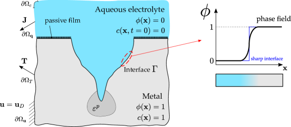
Modelling the moving pit interface requires the application of both Robin (5) and Dirichlet () boundary conditions for the activation-controlled and diffusion-controlled processes, respectively. Instead, we circumvent these complications by following the phase field paradigm proposed by Mai et al. (2016), approximating the interface evolution implicitly by solving for an auxiliary variable . As shown in Fig. 2, the phase field takes values of for the electrolyte and for the metal, varying smoothly between these two values along the interface . Also, for consistency, a normalised concentration is defined as (Mai et al., 2016). Thus, the normalised concentration will equal 1 in the metal (solid) phase, and will approach 0 with increasing distance from the metal-electrolyte interface.
2.2 Principle of virtual work and balance equations
Our theory deals with the coupled behaviour of two systems, one mechanical and one electrochemical one, see Fig. 2. These two systems are coupled by the following physical phenomena: (i) the pit evolution process is accelerated by mechanics, as presented in Eqs. (2) and (3); and (ii) the dissolution of metals leads to a redistribution of mechanical stress. With respect to the mechanical contributions, the outer surface of the body is decomposed into a part , where the displacement can be prescribed by Dirichlet-type boundary conditions, and a part , where a traction can be prescribed by Neumann-type boundary conditions. As for the electrochemical part, the external surface consists on two parts: where the flux is known (Neumman-type boundary conditions), and , where the concentration is prescribed (Dirichlet-type boundary conditions). Accordingly, a concentration flux entering the body across can be defined as . Solute diffusion is driven by the chemical potential , as constitutively characterised below. We follow Duda et al. (2018) in defining a scalar field to determine the kinematics of composition changes, such that
| (7) |
Thus, from a kinematic viewpoint, the domain can be described by the displacement , phase parameter and chemical displacement . We denote the set of virtual fields as and proceed to introduce the principle of virtual work for the coupled systems as,
| (8) | ||||
where is the strain tensor, which is computed from the displacement field in the usual manner and additively decomposes into an elastic part and a plastic part . Also, we use to denote the interface kinetics coefficient, is the phase field microtraction and and are the microstress quantities work conjugate to the phase field and the phase field gradient , respectively. Operating, and making use of Gauss’ divergence theorem:
| (9) | ||||
Finally, considering that the left-hand side of Eq. (9) must vanish for arbitrary variations, the equilibrium equations in for each primary kinematic variable are obtained as
| (10) | |||
with the right-hand side of Eq. (9) providing the corresponding set of boundary conditions on ,
| (11) | |||
2.3 Energy imbalance
The first two laws of thermodynamics for a continuum body within a dynamical process of specific internal energy and specific entropy read (Gurtin et al., 2010),
| (12) | ||||
where is the power of external work, is the heat flux and is the heat absorption. The resulting Clausius-Duhem inequality must be fulfilled by the free energies associated with both systems, mechanical and electrochemical . Thus, the energy imbalances associated with the mechanical and electrochemical systems can be obtained by assuming an isothermal process and replacing the virtual fields by the realizable velocity fields in Eq. (8),
| (13) |
| (14) |
2.4 Constitutive theory
We proceed to define the functional form of free energy of each system and subsequently derive a set of thermodynamically consistent relations.
2.4.1 Constitutive prescriptions for the mechanical problem
The mechanical behaviour of the solid is characterised by von Mises J2 plasticity theory. The extension to strain gradient plasticity (Martínez-Pañeda and Fleck, 2019; Martínez-Pañeda et al., 2019), of particular importance when dealing with sharp pits and cracks, will be addressed in future works. Accordingly, the mechanical free energy is decomposed into elastic and plastic components, both of which are degraded by the phase field,
| (17) |
Here, is the degradation function characterising the transition from the undissolved solid () to the electrolyte phase (). The definition of must satisfy the conditions and ; here,
| (18) |
Consistent with (15), the Cauchy stress tensor is defined as and we denote as the Cauchy stress tensor for the undissolved solid. Thus, accounting for the influence of the phase field and using , the mechanical force balance (10a) can be reformulated as,
| (19) |
where is a small positive parameter introduced to circumvent the complete degradation of the energy and ensure that the algebraic conditioning number remains well-posed. We adopt throughout this work.
The elastic strain energy density is defined as a function of the elastic strains and the linear elastic stiffness matrix in the usual manner,
| (20) |
While the plastic strain energy density is incrementally computed from the plastic strain tensor and the Cauchy stress tensor for the undissolved solid as,
| (21) |
Finally, the material work hardening is defined assuming an isotropic power law hardening behaviour. Such that the flow stress and the effective plastic strain are related by,
| (22) |
where is Young’s modulus, is the yield stress and is the strain hardening exponent ().
2.4.2 Constitutive prescriptions for the electrochemical problem
In the localised corrosion system described in Section 1, the electrochemical free energy density can be decomposed into its chemical and interface counterparts,
| (23) |
The chemical free energy density can be further decomposed into the energy associated with material composition and a double-well potential energy (Mai et al., 2016), such that
| (24) |
where the parameter is the height of the double well potential , and and denote the chemical free energy density terms associated with the solid and liquid phases, respectively. These latter two terms are defined following the KKS model (Kim et al., 1999), which assumes that each material point is a mixture of both solid and liquid phases with different concentrations but similar chemical potentials. Following this assumption, one reaches the following balances
| (25) |
| (26) |
where and are the normalized concentrations of the co-existing solid and liquid phases, respectively. Defining a free energy density curvature , assumed to be similar for the solid and liquid phases, and restricting our attention to dilute solutions, we reach the following definitions for each component of the chemical free energy density,
| (27) |
where and are the normalised equilibrium concentrations for the solid and liquid phases. Combining Eqs. (24)-(27) renders,
| (28) |
On the other hand, the interface free energy density is defined as a function of the gradient of the phase field variable as:
| (29) |
where is the gradient energy coefficient. In the free energy density definitions (28)-(29), the parameters and govern the interface energy and its thickness as:
| (30) |
where is a constant parameter corresponding to the definition of the interface region (Abubakar et al., 2015). The results are sensitive to the choices of and , which characterise the energy barrier that separates the free energy of the coexisting phases.
Finally, the constitutive relations for the associated stress quantities can be readily obtained by fulfilling the free energy imbalance (16), which implies
| (31) |
Thus, the scalar microstress , work conjugate to the phase field , is given by
| (32) |
while the vector microstress , work conjugate to the phase field gradient, reads
| (33) |
Inserting these constitutive relations (32)-(33) into the phase field balance (10b) renders the so-called Allen-Cahn equation:
| (34) |
Eq. (34) shows that material dissolution is governed by the interface kinetics coefficient . The magnitude of can be considered to be a constant positive number (see, e.g., Mai et al., 2016). Here, we assume a time-dependent instead, enriching the modelling capabilities by establishing a relation with our FRDR mechanistic interpretation and our definition of a mechanochemically-enhanced corrosion current density . Thus, from Eqs. (2)-(3) and assuming a linear relationship between and , the interface kinetics coefficient over a time interval is defined as
| (35) |
We emphasise that the interface kinetics coefficient includes the influence of mechanical straining via , and that this is a one-way coupling in that, while reduces the material stiffness, there is no -dependent term in the mechanical problem. Also, we stress that the mechanical free energy density does not contribute to the phase field evolution, see (34). In other words, crack advance takes place due to localised metal loss, as postulated by the slip-dissolution model (see, e.g., Turnbull, 1993). The framework could be extended to incorporate other cracking mechanisms that include a contribution from ; for example, using a coupled framework such as that by Nguyen et al. (2017b).
The material dissolution process (pitting and cracking) can be either activation-controlled or diffusion-controlled, as it will be illustrated in our first case study - Section 4.1. The constitutive choices for the mass transport process are obtained as follows. First, the chemical potential is given by,
| (36) |
Secondly, the flux can be determined following a Fick law-type relation as,
| (37) |
Substituting Eqs. (36)-(37) into the mass transport balance Eq. (10c), the following field equation is obtained
| (38) |
which is an extension of Fick’s second law such that diffusion of metal ions only takes place along the interface and in the electrolyte.
3 Numerical implementation
The finite element method is used to discretise and solve the coupled electro-chemo-mechanical problem. First, we formulate the weak form of the governing equations for the displacement (19), phase field (34), and concentration (38) problems, respectively. Thus,
| (39) |
| (40) |
| (41) |
Using Voigt notation, the nodal variables for the displacement field , the phase field and the normalised concentration are interpolated as:
| (42) |
where denotes the shape function associated with node , for a total number of nodes . Here, is a diagonal interpolation matrix with the nodal shape functions as components. Similarly, using the standard strain-displacement matrices, the associated gradient quantities are discretised as:
| (43) |
Then, the weak form balances (39)-(41) are discretised in time and space, such that the resulting discrete equations of the balances for the displacement, phase field and concentration can be expressed as the following residuals:
| (44) |
| (45) |
| (46) |
where denotes the time step and is the time increment. Subsequently, the tangent stiffness matrices are calculated as:
| (47) |
| (48) |
| (49) |
where is the elastic-plastic consistent material Jacobian.
Finally, the linearized finite element system can be expressed as:
| (50) |
We solve the finite element system by means of a time parametrization and an incremental-iterative scheme in conjunction with the Newton–Raphson method. Good convergence is achieved without the need for staggered schemes; the residual and stiffness matrix components are built using current values and all the equations of the system are solved at once. The numerical model is implemented in the finite element package ABAQUS by means of a user element subroutine (UEL) and Abaqus2Matlab (Papazafeiropoulos et al., 2017) is used for pre-processing the input files. The code, with examples and accompanied documentation, can be downloaded from www.empaneda.com/codes.
4 Results
We proceed to showcase the potential of the model in predicting localised corrosion with five case studies of particular interest. First, in Section 4.1, we validate our predictions with analytical solutions in the context of a pure corrosion problem, the classic benchmark of the pencil electrode test. Secondly, the predictions of the model are compared with experimental measurements of anodic dissolution-driven defect growth in a C-ring test, see Section 4.2. The influence of mechanical contributions in accelerating and governing the pit-to-crack transition in stainless steel is addressed in Section 4.3. Then, the interaction between multiple pits is investigated in Section 4.4 by modelling SCC in a steel plate with pre-existing defects. And finally, the capabilities of the model in conducting large scale 3D simulations of pit corrosion are showcased in Section 4.5.
4.1 Analytical verification under uniform corrosion: pencil electrode test
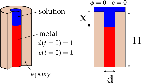
The paradigmatic benchmark of a pencil electrode test is addressed first. This boundary value problem enables validating the numerical framework under pure corrosion conditions, as no mechanical load is applied and no film passivation takes place. The specimen, a H150 m long metal wire with diameter d m, is mounted into an epoxy coating, leaving only one end of the sample exposed to the solution - see Fig. 3. Thus, the problem is essentially one-dimensional and can be described by the change in time of the position of the metal-electrolyte interface .
The evolution of the pit depth can be estimated analytically (Scheiner and Hellmich, 2007), and is found to be proportional to as,
| (51) |
where the unknown is given by:
| (52) |
A proportional dependency of the pit depth on is also observed experimentally (Ernst and Newman, 2002). In both the experiments and the analytical study, corrosion is assumed to be diffusion-controlled; this can be achieved by using a sufficiently large applied potential such that reaction rates are high and the surface concentration reaches a saturation magnitude. Using the phase field method, the pencil electrode test can be conveniently modelled without the need of prescribing a moving Dirichlet boundary condition at the interface (Mai et al., 2016). Thus, as described in Fig. 3 we assign as initial conditions and in the metallic wire and prescribe the Dirichlet boundary conditions and at the pit mouth throughout the numerical experiment. Neumann boundary conditions and are considered at the sides, to simulate the insulation provided by the epoxy coating. The interface kinetics coefficient is assumed to be constant , as there is no mechanical straining or protective film. Following Mai et al. (2016) and Gao et al. (2020), we consider the material and corrosion parameters shown in Table 1; the values listed for the interface thickness and the interface energy result from the choices of a gradient energy coefficient N and a height of double well potential N/mm2, see (30). A uniform finite element mesh is used, with a characteristic element size 10 times smaller than the interface thickness and employing a total of 15,000 quadratic quadrilateral plane strain elements.
| Parameter | Value | Unit |
|---|---|---|
| Interface energy | 0.01 | |
| Interface thickness | 0.005 | |
| Diffusion coefficient | ||
| Interface kinetics coefficient | ||
| Free energy density curvature | 53.5 | |
| Average concentration of metal | 143 | |
| Average saturation concentration | 5.1 |
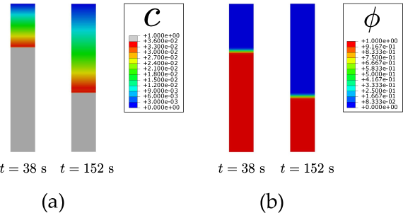
The contours of the phase field and the normalised concentration are given in Fig. 4. Results are shown for two time instants, and s, showing how the metal corrodes and the metal-electrolyte evolves. Fig. 4a shows that the normalised concentration increases from 0 at the pit mouth to at the metal-electrolyte interface; the model captures how a further increase in the pit surface concentration is prevented as saturation occurs.
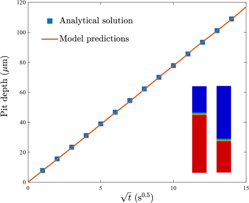
The predictions of the model are quantitatively verified against the analytical solution (51)-(52). As shown in Fig. 5, an excellent agreement is attained in the calculation of the evolution of the pit depth as a function of . The results obtained also coincide with the numerical predictions by Mai et al. (2016) and Gao et al. (2020), further validating our numerical implementation.
We proceed to showcase the capabilities of the model in capturing both diffusion-controlled and activation-controlled corrosion. In the pencil electrode test, the corrosion rate is directly controlled by a non-transient parameter . If is sufficiently high, as in Figs. 4 and 5 (Table 1), the process is diffusion-controlled, with the electrochemical reaction at the metal-electrolyte interface occurring very fast and leading to saturation in the surface concentration of metal ions. On the other hand, if is small, then the corrosion process is activation-controlled and the pit depth shows a linear dependence with time. For a given time instant, e.g. s, one can readily see that increasing the interface kinetics coefficient raises the magnitude of the pit depth, but this sensitivity to is non-linear and saturates as increases; for a sufficiently large value of , further increasing its magnitude has no effect on the corrosion kinetics. Corrosion becomes then diffusion-limited and a higher value of should be adopted to increase dissolution rates.
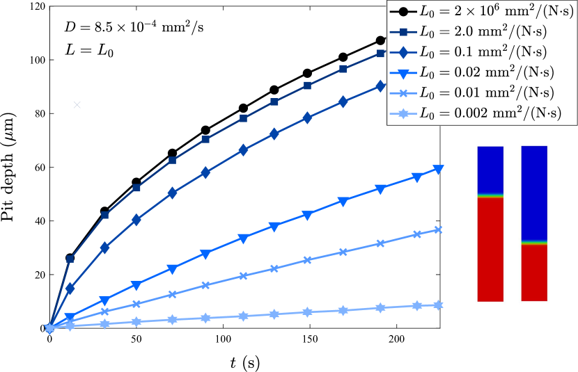
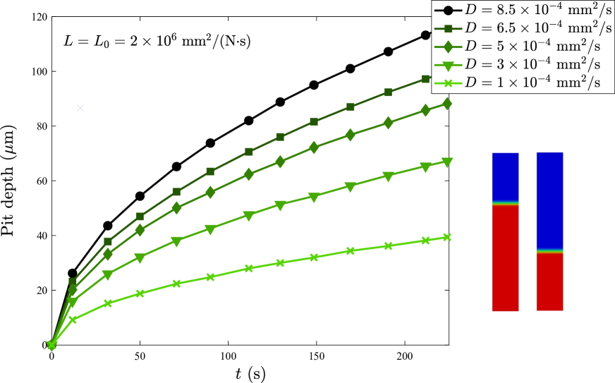
Model predictions of pit growth versus time as a function of the interface kinetics parameter are shown in Fig. 6(a), exhibiting a linear to parabolic trend with increasing . The pit depth evolution is also computed for a large interface kinetics parameter, , and selected values of the diffusion coefficient , see Fig. 6(b). As expected, the corrosion reaction exhibits a significant sensitivity to the magnitude of the diffusion coefficient. As the influence of mechanical straining and film re-passivation and rupture are incorporated, the magnitude of will evolve in time and the transition from activation-controlled to diffusion-controlled corrosion will be captured by the model.
4.2 Chemo-mechanical validation with experiments: C-ring test on Q345R steel
We now verify our model by reproducing the experimental observations by Dai et al. (2020) on C-ring specimens. Q345R steel samples were exposed to a hydrofluoric acid corrosion environment and the growth of pits and associated cracks was quantified for different levels of applied mechanical stress. This choice of environment translates into a negligible influence of film passivation, as the corrosion products are mainly fluorides (not oxides) and the film is not dense enough to prevent the attack of aggressive ions (Dai et al., 2020). The applied strain is held constant throughout the experiment and thus the sensitivity of defect growth rates to mechanical stresses can be quantified. This boundary value problem enables us to validate the chemo-mechanical coupling introduced in our formulation to characterise the interplay between mechanics and corrosion kinetics, see Eq. (3). Note that the sensitivity of corrosion rates to applied stresses cannot be captured with conventional SCC models that restrict the influence of mechanical straining to the local film breakage mechanism (see, e.g., Mai and Soghrati, 2017).
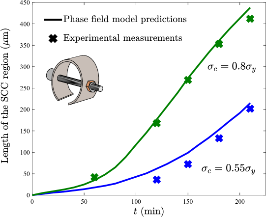
The configuration of the experiment is shown in Fig. 7. The sample is subjected to a constant strain by tightening a bolt centred in the diameter of the ring. The load level is characterised by the circumferential stress at the top of the sample, the region where localised corrosion will develop. Thus, the magnitude of the circumferential stress is determined by placing a strain gauge in the middle of the arc, close to the extreme edge; i.e., in the vicinity of point A, see Fig. 7. The C-ring specimens were exposed to 40 wt.% hydrofluoric acid under room temperature conditions and, using 3D optical microscopy, surface morphologies were characterised as a function of the stress level and the time (Dai et al., 2020).
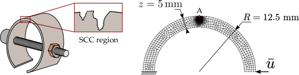
In the finite element model we discretise the domain between the two bolt holes. As shown in Fig. 7, the sample has an inner diameter of 20 mm and an outer diameter of 25 mm. The vertical and horizontal displacements are constrained at the left side, while a Dirichlet boundary condition is used to prescribe the horizontal displacement component of the right side, where the bolt is tightened. The load is prescribed at the beginning of the analysis and then held fixed throughout the calculation. The resulting circumferential stress is measured at the top of the sample (point A), to resemble the experimental measurements. In agreement with the experimental work, we consider a Young’s modulus of GPa, a Poisson’s ratio of and a yield stress of MPa for the Q345R steel. No stress-strain curve or strain hardening exponent is provided in (Dai et al., 2020), a value of is adopted based on the Q345R material characterisation by Liang et al. (2019). The material properties are listed in Table 2.
| Parameter | Value | Unit |
|---|---|---|
| Young’s modulus | 200,000 | MPa |
| Poisson’s ratio | 0.25 | — |
| Yield stress | MPa | |
| Strain hardening exponent | — |
In regard to the corrosion parameters, those listed in Table 1 are used unless otherwise stated. Since no film passivation is involved, we define in Eq. (35). The initial interface kinetics coefficient is chosen so as to provide the best fit to the experimental data; here, . The interface thickness is taken to be mm and the finite element mesh is refined in the SCC region accordingly, with the characteristic element size being equal or smaller than 0.005 mm. A total of 10,681 quadrilateral quadratic elements are used. As shown in Fig. 8, several pits are observed in the experiments, with one of them becoming a particularly large crack - we aim at capturing this dominant localised corrosion defect and address later the occurrence of multiple pits and their interactions. To trigger the dominant localised defect, the Dirichlet boundary condition is prescribed over a length of 0.05 mm in the extreme edge of the middle of the arc (point A). The finite element results obtained in terms of SCC defect length and shape are provided in Fig. 8; the experimental measurements from Dai et al. (2020) corresponding to the same time (210 min) and stress level () are also shown.
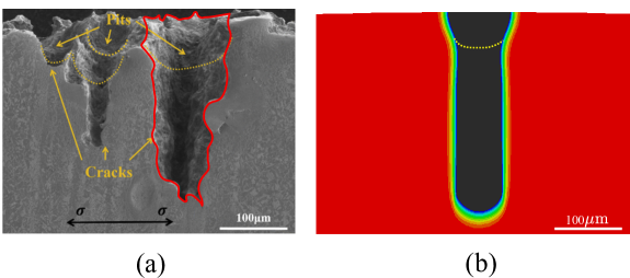
Fig. 8 reveals a good agreement with experimental observations. A quantitative comparison with experiments for different stress levels is provided in Fig. 9. Results are shown in terms of the length of the SCC region, including the initial pitting and subsequent cracking, as a function of time. A very good agreement is observed for both and . We emphasise that while the circumferential stress in the middle of the arc remains below the yield stress, plasticity can develop on the surface of the SCC defects as the resulting notches and cracks act as stress concentrators.
4.3 Parametric study: cracking from a semi-elliptical pit
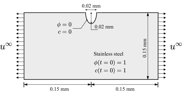
We proceed to conduct numerical experiments on a stainless steel plate, containing a pre-existing pit, to investigate the effect of both mechanical straining and repassivation on the SCC process. The geometric setup, dimensions and boundary conditions are given in Fig. 10. The Dirichlet boundary conditions and are prescribed at the surface of the pre-existing defect, which has a semi-elliptical shape with radii 0.01 and 0.02 mm. At , and are defined as initial conditions in the metallic plate, of height 0.15 mm and width of 0.3 mm. The mechanical load is applied by prescribing a remote horizontal displacement on the left and right edges of the sample, as shown in Fig. 10. The vertical displacement of the top right corner is also constrained to prevent rigid body motion.
The corrosion parameters in this study are those assumed in the pencil electrode test, see Table 1, with the exception of the interface kinetics coefficient; a magnitude of is adopted to ensure activation-controlled corrosion. The constitutive behaviour of the steel plate is characterised by a Young modulus of GPa, a Poisson’s ratio of , an initial yield stress of MPa and a strain hardening exponent of . Approximately 7,000 quadrilateral quadratic plane strain elements are used to discretise the model.
First, we consider the case of mechanics-enhanced corrosion in the absence of a passivation mechanism. The goal is to characterise the role of mechanical straining in controlling the defect growth rate and shape. Thus, we make in Eq. (35) and prescribe three different values of the remote displacement m, m and m. The remote displacement is prescribed at the beginning of the numerical experiment and then held fixed over a total time of 900 s. The results obtained, in terms of the phase field and hydrostatic stress contours, are shown in Fig. 11.
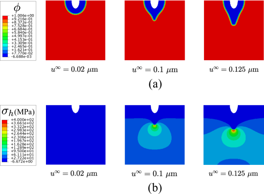
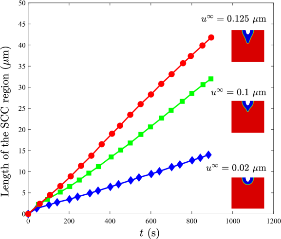
The results reveal that, when the mechanical load is small ( m), there is a negligible influence of the hydrostatic stress and the pit grows approximately the same length in all dimensions, in agreement with the corrosion evolution laws in the absence of mechanical contributions. However as the remote displacement is raised and the magnitude of increases, the pit morphology changes and a pit-to-crack transition is observed. The dominance of the mechanics contributions becomes very clear in the case of m, where the stresses are sufficiently high to trigger plastic deformations and the shape of the SCC defect is governed by both the hydrostatic stress and the plastic strain distribution. It is also worth emphasising that mechanical straining not only sharpens the SCC defect but also increases its length. The length of the SCC region is shown in Fig. 12 for the three chosen values of the applied displacement . It can be seen that the mechanical contribution has a significant effect on localised corrosion rates.
We now turn our attention to the repassivation process and our film rupture-dissolution-repassivation (FRDR) formulation. Thus, we apply and hold fixed a remote displacement of m and consider the sensitivity of the results to changes in the material parameter characterising the corrosion sensitivity to the stability of the passive film, - see Eq. (2) and (35). Three representative values are considered: , , and ; while the critical strain for film rupture and the time interval without repassivation are held constant at and s, respectively.
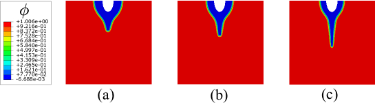
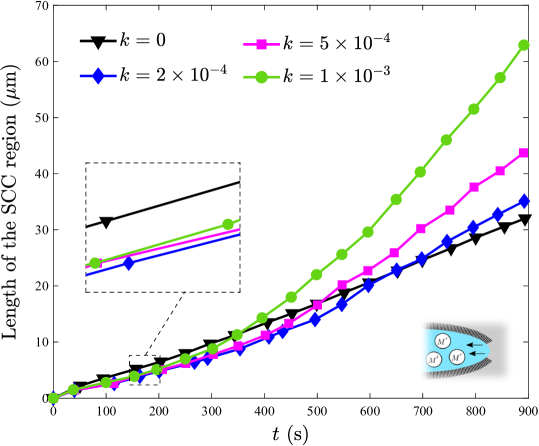
The phase field contours obtained after 900 s are shown in Fig. 13. The impact of in the SCC morphology is evident; higher values accelerate the SCC defect growth rate in the pit base relative to corrosion rates at the pit mouth, sharpening the pit and triggering a pit-to-crack transition. Corrosion rates at the tip of the SCC defect are exacerbated as the defect sharpens and plasticity localises; the protective film is weaker in areas of high mechanical straining - see Eq. (1). The length of the SCC region is shown in Fig. 14 as a function of the film stability parameter , including the case where no film is present (). The results reveal that by introducing the repassivation process, the length of the SCC region drops slightly at an early stage, which is in accordance with the fact that repassivation will restrain the SCC process by decreasing the value of interface kinetics coefficient. After a certain time, the size of the SCC region grows faster with increasing as film rupture occurs and the magnitude of the equivalent plastic strain increases as the defect sharpens, augmenting the interface kinetics coefficient - see Eq. (35).
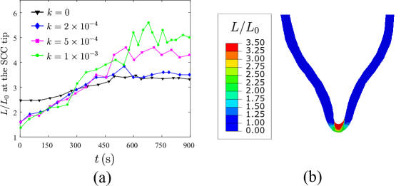
Finally, we gain insight into the model predictions at the local level by quantifying the evolution the interface kinetics coefficient as a function of time and space. We compare the interface kinetics coefficient at the SCC tip to further clarify the local behaviours. First, Fig. 15a shows the evolution in time of the normalised interface kinetics coefficient at the tip of the SCC defect for different values of the film stability coefficient . The initial value of is smaller with increasing due to the effect of film passivation, in agreement with expectations. In all cases, the magnitude of increases with time but eventually reaches a plateau. This indicates that mechanical straining dominates the corrosion process. Also, it is observed that SCC damage becomes more localised as the stability of the film increases. This is showcased in Fig. 15b, where the spatial contour of is shown in the interface region. Higher values of the interface kinetics coefficient are observed at the tip of the pit, where the mechanical fields (, ) are larger.
4.4 SCC driven by the interaction between multiple pits
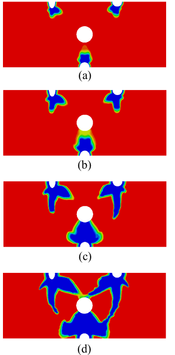
Component failure frequently takes place as a consequence of the interaction between multiple pits. In this section, we demonstrate the capabilities of the model in predicting failure due to the combined action of multiple pits and their coalescence, as well as investigating the role of corrosion parameters in driving the evolution of neighbouring pits. For this purpose, we model a steel plate with an inner defect (not exposed to the environment) and three pre-existing corrosion pits. As shown in Fig. 16, one of the existing pits has a semi-ellipsoidal shape with radii 0.1 and 0.2 mm, while the other two pits have a semi-circular profile and the same radius: 0.15 mm. The mechanical load is applied by prescribing a remote horizontal displacement equal to on each side of the plate. The displacement is prescribed at the beginning of the analysis and held constant afterwards (step function).
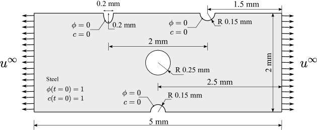
The corrosion and material parameters considered are those listed in Tables 1 and 2, respectively. However, note that a smaller value is assumed for the interface kinetics coefficient, , so as to simulate activation-controlled corrosion. Also, the interface thickness is chosen to be equal to , which is 20 times larger than the characteristic element size. The plate is discretised using 27,450 quadrilateral quadratic plane strain elements with reduced integration. In addition, the presence of a protective film and its rupture is captured by considering a film stability parameter .
The SCC process is shown as a function of time in Fig. 17, where the blue and red colours correspond to the completely corroded and intact areas, respectively. We can see that the three pits increase in depth (Fig. 17a), with the upper two eventually branching (Fig. 17b). The bottom pit eventually coalesces with the central circular defect (Fig. 17c), while the branches of the upper defects sharpen - one growing toward the central defect and the other one in the direction of the bottom pit. Eventually, after approximately 4 hours, the upper and bottom pits merge and complete failure of the plate is predicted (Fig. 17d).
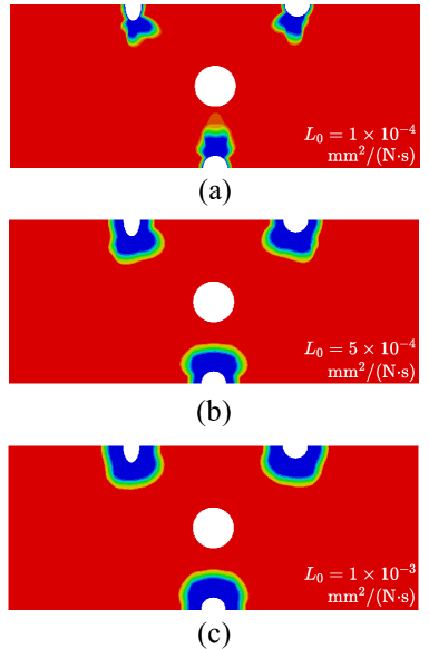
We also compare the SCC morphologies for three different values of to assess the influence of the interface kinetics parameter on the corrosion process. The results are shown in Fig. 18 for a time of =0.5 h. It can be seen that the pits grow more uniformly when the initial interface kinetics parameter is higher, implying a smaller contribution of the mechanical problem with increasing . Mechanical strains and stresses enhance interface kinetics via the mechanochemical term , see (3) and (35). However, this also implies that the mechanical contribution facilitates the transition from activation-controlled corrosion to diffusion-controlled corrosion, and when is sufficiently large such that corrosion is diffusion-limited, corrosion rates become independent of (see Fig. 6(a)) and accordingly of . Consequently, for a given value of the remote load, the contribution from the mechanical problem will be larger for lower magnitudes.
4.5 Three-dimensional predictions of SCC defect growth
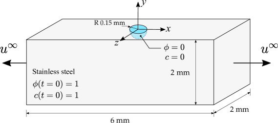
Finally, we extend our computational framework to model 3D SCC problems. The goal is to bring new insight into the mechanics of SCC defect growth and demonstrate the capabilities of our model in addressing technologically-relevant case studies. For this purpose, we choose to model a hemispherical pit in a sufficiently large steel plate subjected to tension, aiming to rationalise the observation of cracks initiating at the cross-section of uniaxial tension samples (Turnbull et al., 2010). The pit, of radius 0.15 mm, has its centre located at 3 mm from the loading edge and at 1 mm along the plate thickness. The geometry, initial and boundary conditions are given in Fig. 19. The remote displacement, applied along the axis, is prescribed at the beginning of the numerical experiment and is held constant throughout the analysis; its magnitude equals mm. The corrosion and material parameters adopted are those listed in Tables 1 and 2 with the exception of an initial kinetics coefficient of , to ensure that at corrosion is activation-controlled. Also, the presence of a protective film is considered, with . The interface thickness is chosen to be mm, which is 20 times larger than the characteristic element size. A total of 356,892 10-node tetrahedral elements are used; the model contains approximately 2.5 million degrees-of-freedom (DOFs).
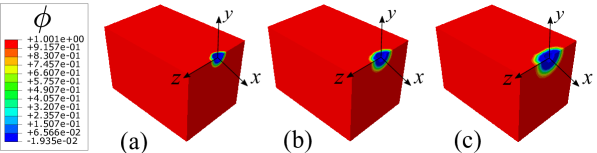
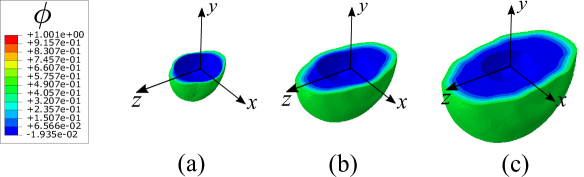
The predicted evolution of the SCC defect is shown in Figs. 20 and 21, in terms of 3D phase field contours. For the sake of a better visualisation, a cut along the - plane is made in Fig. 20 while Fig. 21 shows the SCC region where . It can be observed that the pit tends to grow more along the and directions, relative to the one. This shape evolution of the pit, going from hemispherical to ellipsoidal, is driven by the influence of the mechanical problem. Plastic straining is larger at the pit base and the regions of the pit mouth closer to the cross-section perpendicular to the applied load. Consequently, the magnitude of is larger in these regions and the passive film weaker, leading to an increase in the interface kinetics coefficient. This is in agreement with experimental observations of increasing pit depth and the initiation of lateral cracks (Turnbull, 2001).
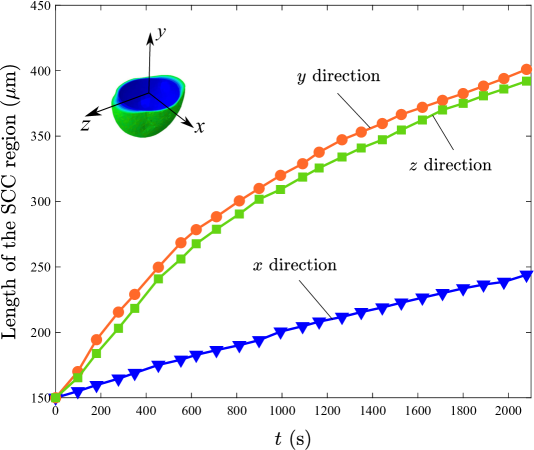
The pit depth along the three Cartesian coordinate axes is shown in Fig. 22 as a function of time. The results show that the pit growth along the direction is linear, i.e. activation-controlled corrosion. However, the results obtained along the and directions transition from linear to parabolic. In other words, the mechanical enhancement of the interface kinetics coefficient has triggered a transition from activation-controlled to diffusion-controlled corrosion. The role of the mechanical contribution will eventually become negligible as raises above its saturation value (diffusion-limited corrosion) but those areas where mechanical straining is higher will continue to corrode faster until reaches its saturation value everywhere, when uniform corrosion will be recovered.
5 Concluding remarks
We have presented a new formulation for predicting dissolution-driven pitting and stress corrosion cracking. Its main ingredients are: (i) a KKS-based phase field model for both activation-controlled and diffusion-controlled corrosion, (ii) a mechanics-enhanced interface kinetics law grounded on mechanochemical theory, and (iii) a strain rate governed film rupture and repassivation process according to the FRDR mechanism. A numerical framework is also presented, with displacements, phase field and concentration of dissolved ions as degrees of freedom. The model is benchmarked by addressing five boundary value problems of particular interest. First, we model the paradigmatic pencil electrode test to verify our numerical implementation and examine the model capabilities in predicting the transition from activation-controlled to diffusion-controlled corrosion. Secondly, we reproduce C-ring experiments in a film-free environment to benchmark our mechanics-enhanced corrosion laws against experimental data. Thirdly, SCC from an ellipsoidal pit is predicted under different conditions to quantify the influence of mechanical stresses and their interplay with the film rupture and repassivation process. Fourthly, the interaction between multiple pits is addressed, assessing the competing influences of the coefficients characterising the mechanical, film stability and interface kinetics contributions. Finally, pit growth in a 3D solid is predicted to showcase the capabilities of the model in capturing large scale phenomena and impacting engineering practice. The main findings are:
-
1.
The interface kinetics coefficient governs corrosion rates. Corrosion kinetics rise with increasing , going from activation-controlled to diffusion-controlled corrosion, until the process becomes diffusion-limited, when corrosion rates become insensitive to a further augmenting .
-
2.
Mechanical stresses and strains enhance corrosion kinetics, in agreement with experiments, favouring localised damage and triggering a pit-to-crack transition. However, if the mechanical enhancement of is sufficiently large, the diffusion-controlled limit is reached and the influence of the mechanical contribution reaches a saturation stage. Thus, the influence of mechanical fields is most notable for activation-controlled corrosion.
-
3.
The presence of a passive film exacerbates localisation and the role of mechanics. The effect is more pronounced if the film stability coefficient is large as film rupture will only occur in regions where mechanical straining is high. Also, cracks are more likely to nucleate under activation-controlled corrosion conditions.
Future developments could involve the extension of the model to consider other cracking mechanisms, including those driven by cathodic reactions. Also, material microstructure and microchemistry can play an important role and should be taken into consideration in many material systems for an accurate prediction of the initial development stages.
6 Acknowledgements
E. Martínez-Pañeda acknowledges valuable discussions with Z.D. Harris (University of Virginia) and A. Turnbull (National Physical Laboratory). Chuanjie Cui and Rujin Ma acknowledge financial support from National Natural Science Foundation of China under grant No. 51878493. E. Martínez-Pañeda acknowledges financial support from the EPSRC (grants EP/R010161/1 and EP/R017727/1) and from the Royal Commission for the 1851 Exhibition (RF496/2018).
References
- Abubakar et al. (2015) Abubakar, A.A., Akhtar, S.S., Arif, A.F.M., 2015. Phase field modeling of V2O5 hot corrosion kinetics in thermal barrier coatings. Computational Materials Science 99, 105–116.
- Anand et al. (2019) Anand, L., Mao, Y., Talamini, B., 2019. On modeling fracture of ferritic steels due to hydrogen embrittlement. Journal of the Mechanics and Physics of Solids 122, 280–314.
- Andresen and Ford (1988) Andresen, P.L., Ford, F.P., 1988. Life prediction by mechanistic modeling and system monitoring of environmental cracking of iron and nickel alloys in aqueous systems. Materials Science and Engineering 103, 167–184.
- Biner (2017) Biner, S.B., 2017. Programming Phase-Field Modeling. Springer.
- Bourdin et al. (2000) Bourdin, B., Francfort, G.A., Marigo, J.J., 2000. Numerical experiments in revisited brittle fracture. Journal of the Mechanics and Physics of Solids 48, 797–826.
- Carrara et al. (2020) Carrara, P., Ambati, M., Alessi, R., De Lorenzis, L., 2020. A framework to model the fatigue behavior of brittle materials based on a variational phase-field approach. Computer Methods in Applied Mechanics and Engineering 361, 112731.
- Chen and Bobaru (2015) Chen, Z., Bobaru, F., 2015. Peridynamic modeling of pitting corrosion damage. Journal of the Mechanics and Physics of Solids 78, 352–381.
- Crane and Gangloff (2016) Crane, C.B., Gangloff, R.P., 2016. Stress corrosion cracking of Al-Mg alloy 5083 sensitized at low temperature. Corrosion 72, 221–241.
- Dai et al. (2020) Dai, H., Shi, S., Guo, C., Chen, X., 2020. Pits formation and stress corrosion cracking behavior of Q345R in hydrofluoric acid. Corrosion Science 166, 108443.
- Duda et al. (2018) Duda, F.P., Ciarbonetti, A., Toro, S., Huespe, A.E., 2018. A phase-field model for solute-assisted brittle fracture in elastic-plastic solids. International Journal of Plasticity 102, 16–40.
- Duddu et al. (2016) Duddu, R., Kota, N., Qidwai, S.M., 2016. An Extended Finite Element Method Based Approach for Modeling Crevice and Pitting Corrosion. Journal of Applied Mechanics 83, 1–10.
- Ernst and Newman (2002) Ernst, P., Newman, R.C., 2002. Pit growth studies in stainless steel foils. I. Introduction and pit growth kinetics. Corrosion Science 44, 927–941.
- Gao et al. (2020) Gao, H., Ju, L., Duddu, R., Li, H., 2020. An efficient second-order linear scheme for the phase field model of corrosive dissolution. Journal of Computational and Applied Mathematics 367, 112472.
- Gurtin et al. (2010) Gurtin, M.E., Fried, E., Anand, L., 2010. The Mechanics and Thermodynamics of continua. Cambridge University Press, Cambridge, UK.
- Gutman (1998) Gutman, E.M., 1998. Mechanochemistry of materials. Cambridge International Science Publishing, Cambridge, UK.
- Gutman (2007) Gutman, E.M., 2007. An inconsistency in ”film rupture model” of stress corrosion cracking. Corrosion Science 49, 2289–2302.
- Hirshikesh et al. (2019) Hirshikesh, Natarajan, S., Annabattula, R.K., Martínez-Pañeda, E., 2019. Phase field modelling of crack propagation in functionally graded materials. Composites Part B: Engineering 169, 239–248.
- Jivkov (2004) Jivkov, A.P., 2004. Strain-induced passivity breakdown in corrosion crack initiation. Theoretical and Applied Fracture Mechanics 42, 43–52.
- Kim et al. (1999) Kim, S.G., Kim, W.T., Suzuki, T., 1999. Phase-field model for binary alloys. Physical Review E - Statistical Physics, Plasmas, Fluids, and Related Interdisciplinary Topics 60, 7186–7197.
- Kristensen and Martínez-Pañeda (2020) Kristensen, P.K., Martínez-Pañeda, E., 2020. Phase field fracture modelling using quasi-Newton methods and a new adaptive step scheme. Theoretical and Applied Fracture Mechanics 107, 102446.
- Kristensen et al. (2020) Kristensen, P.K., Niordson, C.F., Martínez-Pañeda, E., 2020. A phase field model for elastic-gradient-plastic solids undergoing hydrogen embrittlement. Journal of the Mechanics and Physics of Solids 143, 104093.
- Larrosa et al. (2018) Larrosa, N.O., Akid, R., Ainsworth, R.A., 2018. Corrosion-fatigue: a review of damage tolerance models. International Materials Reviews 63, 283–308.
- Liang et al. (2019) Liang, G., Guo, H., Liu, Y., Yang, D., Li, S., 2019. A comparative study on tensile behavior of welded T-stub joints using Q345 normal steel and Q690 high strength steel under bolt preloading cases. Thin-Walled Structures 137, 271–283.
- Lo et al. (2019) Lo, Y.S., Borden, M.J., Ravi-Chandar, K., Landis, C.M., 2019. A phase-field model for fatigue crack growth. Journal of the Mechanics and Physics of Solids 132, 103684.
- Lynch (1988) Lynch, S.P., 1988. Environmentally assisted cracking: Overview of evidence for an adsorption-induced localised-slip process. Acta Metallurgica 36, 2639–2661.
- Macdonald (1999) Macdonald, D.D., 1999. Passivity - the key to our metals-based civilization. Pure and Applied Chemistry 71, 951–978.
- Mai and Soghrati (2017) Mai, W., Soghrati, S., 2017. A phase field model for simulating the stress corrosion cracking initiated from pits. Corrosion Science 125, 87–98.
- Mai et al. (2016) Mai, W., Soghrati, S., Buchheit, R.G., 2016. A phase field model for simulating the pitting corrosion. Corrosion Science 110, 157–166.
- Martínez-Pañeda et al. (2019) Martínez-Pañeda, E., Deshpande, V.S., Niordson, C.F., Fleck, N.A., 2019. The role of plastic strain gradients in the crack growth resistance of metals. Journal of the Mechanics and Physics of Solids 126, 136–150.
- Martínez-Pañeda and Fleck (2019) Martínez-Pañeda, E., Fleck, N.A., 2019. Mode I crack tip fields: Strain gradient plasticity theory versus J2 flow theory. European Journal of Mechanics - A/Solids 75, 381–388.
- Martínez-Pañeda et al. (2018) Martínez-Pañeda, E., Golahmar, A., Niordson, C.F., 2018. A phase field formulation for hydrogen assisted cracking. Computer Methods in Applied Mechanics and Engineering 342, 742–761.
- Nguyen et al. (2017a) Nguyen, T.T., Bolivar, J., Réthoré, J., Baietto, M.C., Fregonese, M., 2017a. A phase field method for modeling stress corrosion crack propagation in a nickel base alloy. International Journal of Solids and Structures 112, 65–82.
- Nguyen et al. (2018) Nguyen, T.T., Bolivar, J., Shi, Y., Réthoré, J., King, A., Fregonese, M., Adrien, J., Buffiere, J.Y., Baietto, M.C., 2018. A phase field method for modeling anodic dissolution induced stress corrosion crack propagation. Corrosion Science 132, 146–160.
- Nguyen et al. (2017b) Nguyen, T.T., Réthoré, J., Baietto, M.C., Bolivar, J., Fregonese, M., Bordas, S.P., 2017b. Modeling of inter- and transgranular stress corrosion crack propagation in polycrystalline material by using phase field method. Journal of the Mechanical Behavior of Materials 26, 181–191.
- Oriani (1972) Oriani, R.A., 1972. A mechanistic theory of hydrogen embrittlement of steels. Berichte der Bunsengesellschaft für physikalische Chemie 76, 848–857.
- Papazafeiropoulos et al. (2017) Papazafeiropoulos, G., Muñiz-Calvente, M., Martínez-Pañeda, E., 2017. Abaqus2Matlab: A suitable tool for finite element post-processing. Advances in Engineering Software 105, 9–16.
- Parkins (1987) Parkins, R.N., 1987. Factors Influencing Stress Corrosion Crack Growth Kinetics. Corrosion 43, 130–139.
- Parkins (1996) Parkins, R.N., 1996. Mechanistic Aspects of Intergranular Stress Corrosion Cracking of Ferritic Steels. Corrosion 52, 363–374.
- Raja and Shoji (2011) Raja, V.S., Shoji, T., 2011. Stress corrosion cracking: theory and practice. Woodhead Publishing Limited, Cambridge.
- Scheiner and Hellmich (2007) Scheiner, S., Hellmich, C., 2007. Stable pitting corrosion of stainless steel as diffusion-controlled dissolution process with a sharp moving electrode boundary. Corrosion Science 49, 319–346.
- Scully (1975) Scully, J.C., 1975. Stress corrosion crack propagation: A constant charge criterion. Corrosion Science 15, 207–224.
- Scully (1980) Scully, J.C., 1980. The interaction of strain-rate and repassivation rate in stress corrosion crack propagation. Corrosion Science 20, 997–1016.
- Serebrinsky et al. (2004) Serebrinsky, S., Carter, E.A., Ortiz, M., 2004. A quantum-mechanically informed continuum model of hydrogen embrittlement. Journal of the Mechanics and Physics of Solids 52, 2403–2430.
- Sofronis and Birnbaum (1995) Sofronis, P., Birnbaum, H., 1995. Mechanics of the hydrogen-dislocation-impurity interactions—I. Increasing shear modulus. Journal of the Mechanics and Physics of Solids 43, 49–90.
- Ståhle and Hansen (2015) Ståhle, P., Hansen, E., 2015. Phase field modelling of stress corrosion. Engineering Failure Analysis 47, 241–251.
- Sun et al. (2014) Sun, W., Wang, L., Wu, T., Liu, G., 2014. An arbitrary Lagrangian-Eulerian model for modelling the time-dependent evolution of crevice corrosion. Corrosion Science 78, 233–243.
- Tanné et al. (2018) Tanné, E., Li, T., Bourdin, B., Marigo, J.J., Maurini, C., 2018. Crack nucleation in variational phase-field models of brittle fracture. Journal of the Mechanics and Physics of Solids 110, 80–99.
- Toshniwal (2019) Toshniwal, D., 2019. Isogeometric Analysis : Study of non-uniform degree and unstructured splines , and application to phase field modeling of corrosion. Ph.D. thesis. The University of Texas at Austin.
- Turnbull (1993) Turnbull, A., 1993. Modelling of environment assisted cracking. Corrosion Science 34, 921–960.
- Turnbull (2001) Turnbull, A., 2001. Modeling of the chemistry and electrochemistry in cracks - A review. Corrosion 57, 175–188.
- Turnbull et al. (2010) Turnbull, A., Wright, L., Crocker, L., 2010. New insight into the pit-to-crack transition from finite element analysis of the stress and strain distribution around a corrosion pit. Corrosion Science 52, 1492–1498.
- Wu et al. (2020) Wu, J.Y., Mandal, T.K., Nguyen, V.P., 2020. A phase-field regularized cohesive zone model for hydrogen assisted cracking. Computer Methods in Applied Mechanics and Engineering 358, 112614.