Multi-scale energy budget of inertially driven turbulence in normal and superfluid helium

Abstract

In this paper we present a novel hydrodynamic experiment using liquid ⁴He. The flow is forced inertially by a canonical oscillating grid using either its normal (He I) or superfluid (He II) phase, generating a statistically stationary turbulence. We characterise the turbulent properties of the flow using 2D Lagrangian Particle tracking on hollow glass micro-spheres. As expected for tracer particles, the Voronoï tessellation on particle positions does not show a significant departure from a random Poisson process neither in He I nor He II phase. Particles’ positions are tracked with high temporal resolution, allowing to resolve velocity fluctuations at integral and inertial scales while properly assessing the noise contribution. Additionally, we differentiate the particles’ positions (by convolution with Gaussian kernels) in order to access small scale quantities like acceleration. Using these measured quantities and the formalism of classical Homogeneous Isotropic Turbulence (HIT) to perform an energy budget across scales we extract the energy injection rate at the large scale, the energy flux cascading through inertial scales, down to small scales at which it is dissipated. We found that in such inertially driven turbulence, regardless of the normal or superfluid state of the fluid, estimates of energy at the different scales are compatible with each other and consistent with oscillating grid turbulence results reported for normal fluids in the literature. The largest discrepancy shows up at small scales where the signal to noise ratio is harder to control and where the 2D measurement is contaminated by the 3D nature of the flow. This motivates to focus future experimental projects towards small scales, low noise and 3D measurements.

I Introduction

Liquid Helium experiments offer a unique way to investigate developed turbulence in laboratory scale facilities. Liquid Helium, in its normal state (He I), has indeed a very low kinematic viscosity $\nu$. Besides, one of the most striking features of liquid Helium is superfluidity (He II) where the kinematic viscosity eventually vanishes below a critical temperature $T_{\lambda}~{}\approx~{}2.17~{}K$.

While He I follows a classical Navier-Stokes equation dynamics for a viscous newtonian fluid, He II is usually described as a mixture of a normal (viscous) and a superfluid (inviscid) components with a relative fraction depending on the temperature (the lower the temperature the higher the superfluid fraction). A consequence of the inviscid nature of the superfluid component is that turbulent eddies in that component cannot have arbitrary circulation: only vortices carrying a single quantum of circulation $\kappa$ may exist, the so-called quantum vortices [41]. Those vortices act as defects where the excitations from the normal component may scatter. This mechanism produces a transfer of momentum between the two components of He II leading to a mechanical coupling called mutual friction.

At finite temperature and in absence of temperature gradient, it is believed that this mutual friction locks the velocity fields of the two components at scales larger than the typical inter-vortex distance $\delta$. That explains the lack of observed difference in energy spectra at large scale [13, 27]. At scales comparable to $\delta$, it is predicted that the mutual friction is not strong enough to lock the two components together hence a different behaviour compared to classical turbulence is predicted [30]. The inter-vortex distance is expected to be of the same order of magnitude as the dissipative scale in the normal component, which may be very small in laboratory experiments (typically ranging between one and several tens of micrometers).

Since Eulerian sensors are difficult to use in He II and do not even exist at scales of less than a tenth of a millimetre, the use of visualization to probe the flow has been explored in the past decades [4, 8] as a promising approach to access quantitative multi-scale diagnosis of quantum turbulence.

$H_{2}$-$D_{2}$ ice particles and hollow grass spheres have initially been used to assess the flow field in counter-flow experiments [19, 2, 22]. Those reveal that Lagrangian statistics at small scales appear to behave differently from those of the conventional fluid [10, 11]. Nevertheless, due to the nature of the counter-flow itself (which has no counterpart in classical fluid), and also to the small level of turbulence involved in this situation, no clear conclusion has emerged yet regarding possible intrinsic differences in the dynamics of super- and normal-fluid turbulence when driven in similar conditions.

More recently, particle tracking velocimetry (PTV) has also been used to measure statistical properties of inertially driven flows. Svancara and La Mantia [34] used $H_{2}$-$D_{2}$ ice particles to look at velocity and acceleration probability density functions in an oscillating grid experiment. They found that the velocity and acceleration distributions were comparable to that observed in standard fluids, as already observed in Eulerian framework for scales larger than $\delta$. Tang et al. [37] studied the velocity structure functions scalings in a towed-grid experiment, in He II only. They conclude, among other, that they observe a larger intermittency than in classical fluids, on the basis of comparison with theoretical models.

It remains unclear at the moment which component the Lagragian particles actually trace in HeII (see e.g. Ref. [12]). One goal of the present study is to proceed to different estimates of energy across scales in order to explore possible deviations to classical behaviors, which may indicate any specificity of superfluid behavior (due either to a preferential sampling of the tracer to one component or the other, or to the existence of different channels for energy to flow and dissipate across scales). To this end, we have estimated the energy rates at different scales, always assuming fundamental laws as they are known for classical fluid turbulence, seeking scale by scale for significant differences between measurements carried in HeI and HeII. This direct comparison is the most reliable way to highlight features peculiar to He II.

To achieve this, we designed a new experimental facility devoted to particle tracking and particle trapping measurements in Oscillating Grid Turbulence [35] (OGT). The main difference with Svancara and La Mantia [34] is that we chose to follow the design rules of a canonical oscillating grid experiments, e.g. grid solidity below 40% and at least 3x3 meshes with half mesh at each end[7, 6, 29]. Thereby our experiment offers the possibility of calibrating and validating our measurements in He I against classical reference data. Compared to grid generated turbulence in wind tunnels, OGT has the advantage to produce a flow with almost no mean flow, hence better suited to particle tracking experiments with fixed cameras. Towed grid experiments, which are now common tools to investigate inertially driven turbulence [33, 44, 37], produce nearly homogeneous isotropic flows but decaying (non-stationary) in time. The choice of OGT for the present study was therefore motivated by its stationarity. It is an important condition as it ensures that energy injection rate, the energy transfer across scales and the energy dissipation rate should compare equal.

In order to have a good control of particle size dispersion, we decided to use hollow glass microspheres. Such particles have a diameter of a few tens of micrometers though (an order of magnitude bigger than ice particles) and part of our study aims at probing the relevance to consider such particles as good tracers.

In section II we present the experimental device. Section III describes the typical experimental protocol to optimise the operation of the facility for particle tracking measurements. Section IV.1 describes particle detection methodology before the exploration of particle trapping in section V. Section IV.2 is dedicated to particle tracking. Finally we present the velocity field in section VI and section VII is devoted to the assessment of the dissipation rate at different scales of the flow.

II Experimental setup

In order to generate inertially driven turbulence in liquid Helium, we designed an oscillating grid experiment together with a dedicated cryostat. The final scope is to access Lagrangian velocity statistics by means of particle tracking experiments in He I and He II and also to investigate eventual preferential concentrations of particles in He II.

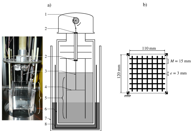
Figure 1: a) Experimental setup: 1- crankshaft + gear-motor system, 2- ball bearing, 3- composite main shaft, 4- grid, 5- test section (“aquarium”), 6- inner (Helium) double wall glass vessel, 7- outer (Nitrogen) double wall glass vessel, 8- Aluminum radiation shield. b) Details of the grid and test section dimensions

Fig. 1-a presents a simplified sketch view of the experiment with the main elements of the facility.

In the sequel we will first detail the turbulence generation system, then describe the cryostat and the visualization setup, and finally the particle seeding technique.

II.1 Turbulence generation

Turbulence is produced by oscillating a grid (item 4 in a fig. 1-a) in a liquid helium bath (light gray). The grid is driven by a gear motor (1), inside the cryostat but at room temperature, via a shaft (3) which is designed to minimize heat losses due the thermal gradient.

The motor is a MDP EC40 equipped with a planetary gear head GP 42 C with a reduction ratio of 26:1. The system has a maximal rotation frequency of $6.4\text{\,}\mathrm{H}\mathrm{z}$ and can deliver a maximal torque of $4.2\text{\,}\mathrm{N}\,\mathrm{m}$. During the experiments presented in this paper, the grid was always driven at constant frequency $f=$5\text{\,}\mathrm{H}\mathrm{z}$$.

We use a crankshaft with an adjustable stroke $S$ to convert the rotation to quasi-sinusoidal vertical translation. The maximal stroke is about 30 mm, but experiments exposed in this paper were all performed with $S=1.77\,M\approx$26\text{\,}\mathrm{m}\mathrm{m}$$.

The grid oscillates vertically in a glass box (item 5 in fig. 1-a) with square cross-section immersed in the bulk of liquid Helium. The sides of the box are $W=$120\text{\,}\mathrm{m}\mathrm{m}$$ large (marginally larger than the grid itself, see fig. 1-b) and the height is $H=$250\text{\,}\mathrm{m}\mathrm{m}$$. The top and bottom ends of the box are open: the goal of this "aquarium" is to ensure a reproducible turbulence generation region, with well controlled boundary conditions. The open top and bottom help in minimizing recirculating flows, although some residual large scale mean recirculations are known to be hardly avoidable in oscillating grid experiments. The four side walls of the aquarium are made of glass for optical access purposes.

II.1.1 Grid Geometry

Fig. 1-b shows the grid geometry. It has been designed based on previous studies in classical fluids in order to respect canonical conditions on the solidity and the end conditions [6], known to produce a well characterized turbulence, with good homogeneity and isotropy properties.

The grid is made of anodized aluminum with square bars and has a solidity $G\approx 36\%$. As a reminder, the solidity $G$ is defined as the ratio between the frontal area effectively blocked by the bars and the total cross section area of the grid, which for a square grid as ours can be simply related to the bar width $e$ and the mesh size $M$:

$$G=\frac{e}{M}\left(2-\frac{e}{M}\right).$$ (1)

When the grid solidity exceeds 40%, the jets and wakes produced by the oscillation of the grid are known to become unstable and merge together to form larger structures [7]. We have chosen a solidity of 36% ($e=$3\text{\,}\mathrm{m}\mathrm{m}$$, $M=$15\text{\,}\mathrm{m}\mathrm{m}$$) for which "the wakes coalesce with each other without bending their axes; shear-free turbulence can be expected on either side of the grid at sufficiently large z" [28].

Table 1 summarizes the grid characteristics.

Grid
$M$	$e$	$G$	$f$	$S$
[mm]	[mm]	[%]	[Hz]	[mm]
15	3	36	5	26

Table 1: Grid characteristics : $M$ : mesh size, $e$ : grid bar thickness, $G$ : solidity, $f$ : frequency, $S$ : stroke.

II.1.2 Expected flow characteristics

From the chosen grid parameters, it is possible to estimate the expected flow characteristics, by means of empirical laws. The integral length scale $L$ increases linearly with the distance to the grid $z$:

$$L~{}=~{}c_{L}z$$ (2)

where $c_{L}$ is a constant that depends upon the grid geometry. For comparison we will use $c_{L}=0.2\pm 0.05$, which is the values Hopfinger and Toly [7] obtained with $S/M=8/5$, the closest to our configuration.

For simplicity, we define the origin of the vertical coordinate $z$ as the midpoint of the oscillation even though Hopfinger and Toly [7] report virtual origins of order $M$.

The transverse (horizontal) fluctuating velocity $\sigma_{u}$ has been shown to follow:

$$\sigma_{u}~{}=~{}c_{u}fM^{1/2}S^{3/2}z^{-1}$$ (3)

where $c_{u}$ is a constant that depends upon the grid geometry. Based on the literature [7, 28] we consider $c_{u}=0.25$. The fluctuating velocity decreases as the inverse of the distance $z$.

In the sequel we will also measure the dissipation rate per unit mass of the flow $\epsilon$. In previous grid experiments, it has been shown to behave as:

$$\epsilon~{}=~{}C_{\epsilon}~{}\frac{\sigma_{u}^{3}}{L}$$ (4)

where $C_{\epsilon}~{}\approx~{}1$ [31].

Assuming that the flow is quasi homogeneous and isotropic, from the dissipation rate one can then infer the Kolmogorov dissipative length scale

$$\eta~{}=~{}\left(\frac{\nu^{3}}{\epsilon}\right)^{1/4}$$ (5)

It is generally unclear how exactly the kinematic viscosity $\nu$ should be defined in He II flows. Babuin et al. [1] have measured an effective viscosity $\nu_{\text{eff}}$, defined as the ratio between the dissipation rate and the mean enstrophy, in a turbulent grid flow. They found that around 2 K, the value of $\nu_{\text{eff}}$ is of the same order of magnitude as $\mu_{n}/\rho$ where $\mu_{n}$ is the dynamic viscosity of the normal component. In the sequel, we thus use $\nu=\mu_{n}/\rho\approx 1\times 10^{-8}\,\mathrm{m^{2}/s}$ as an approximation in He II.

Table 2 summarizes the above primary and derived quantities in our experimental conditions.

a) $L$ $\sigma_{u}$ [mm] [mm/s] $14\pm 5$ $9.3_{-1.9}^{+2.6}$

b) T P $\epsilon$ $Re_{\lambda}$ $\eta$ $\tau_{\eta}$ [K] [bar] [$10^{-5}\mathrm{m^{2}/s^{-3}}$] [-] $\mu$m [ms] 2.8 1 $5.8_{-3.7}^{+12.2}$ 280 22 20 3.5 1 $5.8_{-3.7}^{+12.2}$ 270 24 21 2 0.031 (sat) $5.8_{-3.7}^{+12.2}$ 440 - -

Table 2: Expected flow characteristics. a) Primary quantities obtained from correlations[2,3] at $f=5Hz$, $\frac{S}{M}=1.77$, $\frac{z}{M}=4.6$. The main assumption is that the energy injection at large scale does not depend on the fluid. The uncertainties are computed considering min and max values of $z$ in the field of view together with reported uncertainties on $c_{L}$ and $c_{u}$.
b) Derived quantities: $\epsilon$ from eq. 4, $Re_{\lambda}$ : Reynolds number based on the Taylor length and is obtained under the assumption of homogeneity and isotropy of the flow as $Re_{\lambda}=\sqrt{15L\sigma_{u}/\nu}$, $\eta$ Kolmogorov length scale, $\tau_{\eta}$ : Kolmogorov time scale.

II.2 Cryostats

Usually, visualization experiments in cryogenic facilities are performed in stainless steel cryostats with small planar optical accesses to minimize heat losses in the Helium bath [2, 10, 25]. However, the field of view is then limited by the number of available windows and by the diameter of the windows. We have chosen for our facility to use glass (rather than stainless steel) as material for the cryostat, in order to have a higher level of versatility for visualization purposes. For instance, although we only present here 2D measurements, a glass cryostat with full optical access, allows to consider in future campaigns multi-camera experiments for simultaneous recordings at several viewing angles, hence allowing well resolved 3D particle tracking measurements. The use of a glass cryostat has the additional benefit of being less expensive than the mixed stainless steel/glass solution, as it avoids the requirement of sophisticated welding between a stainless-steel cryostats and optical accesses.

Two cylindrical concentric double-wall glass vacuum cryostats are used. The inner cryostat contains the liquid Helium bath, where the turbulence is generated. The outer cryostat contains liquid nitrogen, and plays the role of thermal shield to limit losses between room temperature and the bulk of liquid Helium. Glass is naturally opaque to the infrared radiations and is heated by room temperature radiations and in turn heats up the liquid nitrogen hence producing bubbles. These bubbles disturb the visualization through the cryostats. To avoid this perturbation, the level of nitrogen is kept below the visualization area during operation of the experiment. This in turn reduces the efficiency of the Nitrogen thermal shield. To further minimize radiation heat load, an aluminum shield (item 8 in fig. 1-a) is also immersed inside the liquid nitrogen cryostat. Holes are made in the aluminum shield at the level of the visualization area. Note that this aluminum shield is disposable and a new adapted shield can easily be prepared if cameras are added to the experiment or if the visualization area needs to be enlarged.

II.3 Visualization system

Measurements are based on high-speed visualization with a Phantom V12 camera (with a maximum frame rate of 6200 images per second at the highest resolution of 1280 pixels $\times$ 800 pixels on a one inch CMOS sensor). We use a red Light Emitting Diode (LED) with a collimation lens in order to produce an approximately parallel light beam aiming straight on the camera lens as shown in fig. 2.

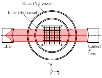
Figure 2: Top view of the visualization system.

In this backlight configuration, we record the shadows of the particles travelling across the light beam, with an a priori undetermined position in the $y$ direction (along the line of sight of the camera). We therefore use a lens with a large numerical aperture (a long distance microscope K2-SC CF-1/B) that ensures both a good luminosity (and contrast) and a small depth of field. The latter has been measured to be of the order of $\delta_{dof}\simeq 1.4$ mm, hence ensuring a quasi-2D measurements at a fixed known $y$-position. Besides, the backlight configuration allows for a good contrast with a low light power, which minimizes the heat sources into the helium bath.

All the measurements discussed here have been done at a vertical position centered around a distance $z=4.6\,M$ below the average position of the grid. The overall field of view is $1.8M\times 1.2M$ (i.e. $25\times 18$ mm²). The camera lens was located at a working distance of $35.5\text{\,}\mathrm{c}\mathrm{m}$ from the center of the aquarium. The geometrical configuration is the same in He I and in He II.

II.4 Particles

Particle seeding was done using K20 type hollow glass microspheres from 3M. Those particles are commercially available as a poly disperse population with sizes ranging from 10 to $200\text{\,}\mu\mathrm{m}$ and densities ranging from 130 to $200\text{\,}\mathrm{k}\mathrm{g}\,\mathrm{m}^{-3}$.

We first sieved those particles in order to remove the largest and the smallest ones. Only particles that have a diameter larger that $71\text{\,}\mu\mathrm{m}$ and smaller than $100\text{\,}\mu\mathrm{m}$ have been retained for our measurements. The particle size distribution has then been measured using a Spraytech diffractometer from Malvern Instruments Ltd. The particle mean diameter D32 (defined as the ratio between the mean volume and the mean area) has been found to be of the order of $85\text{\,}\mu\mathrm{m}$.

We also measured the average particle density: we immersed a know mass of particles in a known volume of water, and measured the resulting total volume. We found a mean particle density of the order of $177\text{\,}\mathrm{k}\mathrm{g}\,\mathrm{m}^{-3}$.

Table 3 summarises the particle characteristics.

Material	$\Phi_{p}$	$\rho_{p}$
[-]	[$\mu$m]	[kg/m3]
hollow glass	85 $\pm$ 15	177 $\pm$ 45

Table 3: Particles characteristics : $\Phi_{p}$ : mean diameter, $\rho_{p}$ : mean density

Finally, we observed the shape of the particles with a binocular and verified that they were spherical except for a small fraction corresponding to broken particles. These pieces of sphere were no longer hollow and contributed to a slight increase in overall density, so that the value of $177\text{\,}\mathrm{k}\mathrm{g}\,\mathrm{m}^{-3}$ is a maximum value. During the experiment, the broken particles sank rapidly after injection.

Particles are dried and injected in the flow using a removable cryogenic syringe. A few minutes before recording data, we start oscillating the grid. This has two main advantages: (i) the flow reaches a steady state and (ii) dense or broken hollow micro-spheres settle and only particles with a density close to the density of the fluid stay in our visualisation field. Typically we estimate that the difference between particles density and fluid density is lower than 15%.

III Experimental Procedure

As mentioned in the introduction, we aim at performing experiments both in normal He I and superfluid He II. From a cryogenic point of view, a fundamental difference between these two states of liquid Helium concerns the heat conductivity. While He I has a very low thermal conductivity (e.g. $0.02\text{\,}\mathrm{W}\,\mathrm{m}^{-1}\,\mathrm{K}^{-1}$ at $3\text{\,}\mathrm{K}$ and $1\text{\,}\mathrm{b}\mathrm{a}\mathrm{r}$), He II has a very high effective thermal conductivity. As a consequence, a He II bath is quasi isothermal, as opposed to a He I bath.

If the free surface of liquid Helium is at saturation pressure $P_{\text{sat}}(T_{\text{free-surf}})$, in absence of a temperature gradient in the fluid, any point below the free surface is sub-cooled due to the pressurization resulting from the immersion depth. In He II it is reasonable to assume there is no temperature gradient and the liquid is therefore always sub-cooled. This ensures that no bubbles can appear and perturb the flow.

On the contrary, He I has a low thermal conductivity and the temperature of the liquid below the free surface can increase due to parasitic heat inputs (through the walls). Those temperature differences can easily overcome the sub-cooling due to the immersion depth, resulting in boiling inside the bath.

In order to avoid the presence of bubbles in the field of view, the following procedure is applied for He I experiments. After filling with liquid helium, the bath is cooled down to 2.4K by pumping, the liquid level being kept well above the top of the test section. Then, helium gas at atmospheric pressure is reintroduced above the liquid interface enabling pressurization and stratification (cold liquid is denser and remains at the bottom). This pressurization process gives enough time to perform quasi-stationary measurements in He I without bubbles: we can typically have half an hour at the operating grid frequency (5 Hz) before the temperature at the visualization level reaches the saturation temperature ($\approx$4.2\text{\,}\mathrm{K}$$) generating bubbles again.

In He II, a MKS 600 valve is used to control the bath pressure (hence the temperature). As previously mentioned, the grid is oscillated a few minutes before taking measurements in order to ensure a steady state is reached [14]. For the three explored experimental condition (see tab. 4), at least 80 films of 400 images are recorded to achieve a good statistical convergence. To resolve particle dynamics, the sequences of 400 images are recorded at a frame rate $F_{s}=3000$ frames per second so that $\delta t\ll\tau_{\eta}$ where $\tau_{\eta}$ is the dissipative Kolmogorov timescale of the flow (previously estimated in table 2) and $\delta t=F_{s}^{-1}$ the time between two images. Typically we have 60 frames per $\tau_{\eta}$.

Furthermore, images extracted from different films can be considered as uncorrelated as the delay between two consecutive films is $20\text{\,}\mathrm{s}$, which is greater than the integral time of the flow ($1.4\text{\,}\mathrm{s}$)

The different test conditions explored in this paper consist in three different different configurations that are summarized in table 4.

Config.	Fluid	$T$	$\rho_{f}$	$f$
[-]	[-]	[K]	[kg/m3]	[Hz]
1	He I	2.8$\pm 0.1$	145.0	5
2	He I	3.5$\pm 0.1$	138.0	5
3	He II	2	147.5	5

Table 4: Experimental conditions : $T$ the temperature, $\rho_{f}$ the density of the carrier fluid, $f$ the oscillating frequency of the grid.

IV Image processing

In this section we describe how the image sequences are post processed to first determine the position of individual particles at a given time $t$, and then to reconstruct tagged particle tracks along time.

IV.1 Particle detection

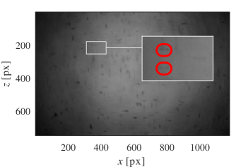
Figure 3: Raw Image with a zoom on ghost particles. Field of view of 1280pixel x 800pixel.

Fig. 3 shows a typical raw image of the hollow microspheres to be tracked in the oscillating grid flow. This image shows important optical distortions which may affect particle detection and eventually the accuracy of the overall particle tracking procedure. It can indeed be seen that out of focus particles are strongly distorted, with either a vertical or a horizontal image. This anisotropic distortion is classical of a cylindrical lens effect, very likely induced by the cylindrical double walls of the inner and outer cryostats. The main goal of the image post-processing is to correctly detect the particles which are in focus.

The overall image processing sequence is as follows. First, to clean images, we apply morphological opening of the image, in order to retrieve the slightly inhomogeneous background illumination, which is subtracted from the corresponding image. Second, a thresholding is applied to select the most contrasted particles; this eliminates most particles that are out of the depth field, as they are dimmer. Finally, in focus particles are often found to exhibit a pattern with multiple (typically 3) images closely aligned in the horizontal direction. This is very likely due to multiple reflections between the walls of the concentric cryostats. To remove this effect, a morphological closing using a small horizontal segment is used to connect dark pixels (we recall that particles appear dark on a bright background) that are closer from each other by less than 5 pixels (i.e. $100\text{\,}\mu\mathrm{m}$). This leads to processed image were most in focus particles appear as smooth blobs of pixels. Their center is determined as the center of mass of these blobs, see fig. 4.

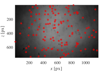
Figure 4: Detection of particles in the raw image from fig. 3.

IV.2 Particle Tracking

Once particles are identified (typically we have an average of 80 particles per image), they are tracked to get their trajectory along time. For this we perform Lagrangian Particle Tracking using the particle tracking code by Nicholas Ouellette[21].

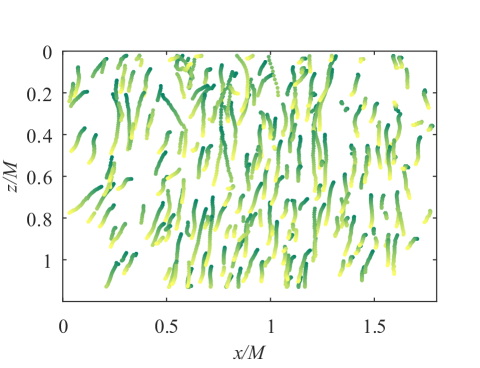
Figure 5: Particle trajectories over 400 images in He II (config. 3 in tab. 4). Dark green is for t = 0 and light green relates to the end of a video (400^th image) at t = 133ms.

In fig. 5, we show typical trajectories obtained after particle tracking over a sequence of 400 images.

Lagrangian velocity and acceleration are obtained by convolution of the raw trajectories with a truncated Gaussian smoothing and differentiating kernel [16] to filter high frequency noise from the recorded trajectories. Traditionally, the width of the filtering kernel is chosen as to minimize the impact of noise on acceleration variance [17, 36, 20, 9]. However, the level of small scale noise is particularly high in our experiment compared to classical experiments at ambient temperature, due to the multiple curved optical interfaces between the core of the cryostat and the cameras. As a consequence, the typical time scales of the noise, overlap with the small turbulent dynamics of the particles and estimates of acceleration remain sensitive to the choice of the filtering width, what affects the robustness of acceleration statistics (see section VII.3). Future experiments are planed to improve this, by an entirely new design of the cryostat in order to avoid multiple layers of curved interfaces. For the present study, we therefore chose the filtering properties based on particles velocity variance, which is less sensitive to small scale noise than acceleration. We find that a Gaussian smoothing kernel of width 6 ms limits reasonably the impact of noise with a weak impact on velocity estimates.

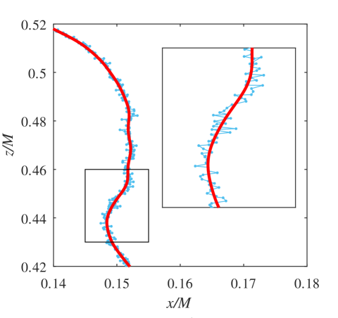
Figure 6: Particle trajectory filtered with a Gaussian kernel of width 18 points (6 ms).

Fig. 6 represents an example of such raw and filtered trajectory, clearly showing the high degree of small scale noise. As discussed in sec VI.2, even after this filtering procedure velocity increment statistics at inertial scales may still be weakly affected by some remaining level of noise. This lead us to deploy a strategy in order to access robust statistical estimate of the Lagrangian dynamics of the particles based only on their position (and position increments) statistics, hence avoiding the amplification of noise associated to numerical differentiation (see section VI.2 and section VII.2.1).

V Preferential concentration study

The flow conditions explored here lead to a Kolmogorov scale (in He I) of the order of $23\text{\,}\mu\mathrm{m}$. According to Babuin et al. [1], we expect that the inter-vortex distance should be of the same order. Thus, the $80\text{\,}\mu\mathrm{m}$ micro-spheres used here are also of the same order of magnitude. In addition, the microspheres that remain in the field of view after a certain delay have a density very close to the density of the fluid. These particles can therefore be expected to behave like tracers and be randomly distributed in space. In this section, we will verify this in He I, a classical fluid.

Contrary to ideal tracers, which follow the flow and are randomly distributed, inertial particles may experience clustering (see e.g. Monchaux [15]). On the other hand, even for tracer particles, preferential concentration may arise in He II due to the trapping of particles about the core of the quantized vortices. This phenomenon has been widely studied by direct visualisation of turbulent counter-flow experiments [45, 18, 22, 23] in He II at rest, but has never been addressed in mechanically forced superfluid turbulence.

We propose in the sequel an original analysis (based on Voronoï tesselations) of the spatial distribution of the detected particle centers in order to explore whether particles exhibit some non-trivial structuration. A Voronoï diagram consists in defining a cell that contains all the points of the space that are closer to a given particle than to any other particle. Fig. 7 presents the Voronoï diagram of particles detected in fig. 4.

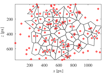
Figure 7: Voronoï diagram of particles detected in fig. 4.

In regions where there are a lot of particles, Voronoï cells have a small area and where there are few particles, cells are bigger: the inverse of cell areas reflects the particles concentration. Hence, the cell areas Probability Density Function provides a quantitative way to describe the degree of clustering of a set of particles. This method of analysis of particle preferential concentration has already been widely used but to the authors’ knowledge never on He II seeding. We applied this method to our measurements both in He I and in He II.

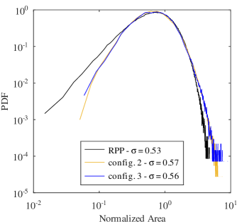
Figure 8: Probability Density Functions of normalized Voronoï area: Random Poisson Process (black), config. 2 (orange) and config. 3 (blue).

In fig. 8, the black curve is the PDF of the voronoï cell areas in the case of randomly distributed particles. This kind of distribution can be modeled by a Random Poisson Process (RPP) which has a standard deviation $\sigma\approx 0.53$. The blue and orange curves are the PDF of voronoï areas in He I and He II respectively. The curves follow the same trend within the accuracy of our measurements, so the distribution of particles does not depend on the state of helium. Furthermore the PDF in He I and He II both have a standard deviation $\sigma$ comparable to that of the RPP. This means that the distribution of the particles is almost random as expected for a homogeneous seeding and tracer particles.

We have done further tests that show that the PDF obtained in He I do not depend on the height $z$ either. This demonstrates that the position of the injector is sufficiently far away to avoid any residual preferential concentration.

In conclusion, this Voronoï diagram method has the double benefit of analyzing particle trapping and investigating the nature of particles in the flow.

At this point, it is interesting to have an estimate of the inter vortex line distance $\delta$. Following Babuin et al. [1], we can use evaluate the effective viscosity which leads to $\delta\approx$35\text{\,}\mu\mathrm{m}$$.

In our working conditions, i.e. with particles of diameter $d_{p}\approx$85\text{\,}\mu\mathrm{m}$$, slightly larger than the inter-vortex distance, the analysis provided no evidence for particle trapping in He II. The particles are unlikely to be influenced by a single vortex and it would thus be interesting to study the case where $d_{p}\ll\delta$.

VI Single Time Velocity Statistics

Fig. 5 shows a typical set of reconstructed trajectories. An overall vertical trend of particles motion can be seen which suggest the existence of a mean drift velocity, see [5, 14]. This is expected as particles are slightly denser than the carrier fluid, see Table 5. Besides, to get a zero mean velocity in an oscillating grid experiment, an infinite aspect ratio of the aquarium for the test section $H/W$ is required. In the horizontal direction, where the gravity should have no effect, the mean velocity $\langle~{}u~{}\rangle$ has been measured and found to be negligible compared to velocity fluctuations. The ratio between the average and the standard deviation of the velocity is $\langle u\rangle/\sigma_{u}\approx 0.1$ in He I and $\langle u\rangle/\sigma_{u}\approx 0.3$ in He II. In the next sections we focus the analysis on the horizontal component $u$ of the velocity.

VI.1 Velocity Probability Density Function and classical fluctuating velocity computation

Fig. 9 shows the probability density function (PDF) of the horizontal velocity fluctuations. They are found to be quasi-gaussian, with slightly over-gaussian tails. Table 5 summarises the trends of the standard deviation of velocity and its comparison with the expected value from classical empirical laws usually used for oscillating grids in classical fluids (Eq. 3). A good agreement is found with the empirical law, with no major difference between the fluid and the superfluid cases. A small difference is observed however between the 2 measurements performed in He I: config. 1 shows a larger deviation to empirical laws.

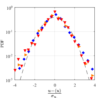
Figure 9: Probability Density Function of normalized velocities alongside the horizontal axis $x$: $\blacktriangledown$ : config. 1 / $\color[rgb]{1,.5,0}\blacktriangleright$ : config. 2 / $\blacklozenge$ : config. 3.

Config.	Fluid	$\sigma_{u}$	$\langle u\rangle$	$\frac{\sigma_{u}}{\sigma_{u}^{th}}$
[-]	[-]	[mm/s]	[mm/s]	[-]
1	He I	8.3 $\pm$ 1.7	0.9	0.86
2	He I	9.3 $\pm$ 1.9	0.3	0.96
3	He II	9.1 $\pm$ 1.8	-3.2	0.94

Table 5: Summary of horizontal velocity measurements obtained using position differentiation.

VI.2 An alternative way to access the fluctuating velocity

Lagrangian velocity is usually obtained from the derivative of individual particle trajectories (see previous section VI.1). Statistics are then estimated from this data set of individual velocities. Such a numerical differentiation process on individual trajectories tends to amplify the noise present in the position data of the particles and requires to filter the trajectories. As described in section VI.1 this is done here using gaussian-filtering. Choosing appropriate filtering parameters is not trivial : if individual trajectories are not sufficiently filtered the statistical quantities estimated (as the velocity standard deviation) may be biased as they still include noise contributions, whereas if the trajectories are too filtered, they will be artificially smoothed.

We propose here an alternative estimation of the standard deviation of the particle velocity based on purely kinematic considerations of the position temporal increments $\delta x$. This approach does not require filtering individual trajectories and hence gives a more robust estimate.

Let’s consider the mean square displacement of the particles $\delta x^{2}=\langle\left(x(t)-x(t+\tau)\right)^{2}\rangle$ where $x(t)$ and $x(t+\tau)$ represent the horizontal position at two different times of the same particles along its trajectory. Assuming the trajectories are smooth (and differentiable) for sufficiently small timelags while they become uncorrelated and non-smooth for large timelags, the mean square displacement is expected to have at least two asymptotic regimes :

$$\langle\delta x^{2}\rangle=\left\{\begin{array}[]{r c l}u_{rms}^{2}\tau^{2}&\,\text{for}&\tau~{}\ll~{}T_{L}\\ 2u_{rms}^{2}T_{L}\tau&\,\text{for}&\tau~{}\gg~{}T_{L}\end{array}\right.$$ (6)

where $u_{rms}^{2}$ is the second-order moment of the velocity and $T_{L}$ represents the Lagrangian correlation time scale of the particles motion. In our study the duration of a video (133ms) is shorter than the integral time $T_{L}=1.4s$, hence only the short term ballistic regime $\langle\delta x^{2}\rangle~{}=~{}u_{rms}^{2}\tau^{2}$ is expected to be observed.

In practice, experimental data of particles position do not exhibit a smooth ballistic regime at the smallest time scales, because of the presence of experimental noise. This results in a deviation from the quadratic dependence $\delta x^{2}\propto\tau^{2}$ for the smallest $\tau$. For a purely uncorrelated noise, mimicking perfect brownian motion at short time scales, one would expect to see $\delta x^{2}\propto\tau$. To model the influence of noise, the measured particle position $x$ can be written as the sum of the real position $x^{*}$ (without noise contribution) and the experimental noise $\theta$: $x=x^{*}+\theta$. The measured mean square displacement can then be rewritten, for the short time lags, as

$$\langle\delta x^{2}\rangle=u_{rms}^{2}\tau^{2}+2\langle\theta^{2}\rangle\left(1-R_{\theta\theta}\left(\tau\right)\right)+\mathcal{O}(\tau^{3}),$$ (7)

where $R_{\theta\theta}$ is the autocorrelation function of the noise:

$$\lim_{\tau\to 0}R_{\theta\theta}(\tau) = 1,$$ (8)

$$R_{\theta\theta}(\tau\gg\tau_{\theta}) = 0.$$ (9)

Here $\tau_{\theta}$ is the correlation time scale of the experimental noise.

From eq. 7, by replacing $u_{rms}^{2}$ by $\langle u\rangle^{2}+\sigma_{u}^{2}$, hence not necessarily assuming the mean velocity $\langle u\rangle$ is zero, one sees that the standard deviation of the velocity $\sigma_{u}$ can be estimated from the measured mean square displacement:

$$\langle\delta x^{2}\rangle-\langle{u}\rangle^{2}\tau^{2}=\sigma_{u}^{2}\tau^{2}+2\langle\theta^{2}\rangle\left(1-R_{\theta\theta}\left(\tau\right)\right)+\mathcal{O}(\tau^{3}).$$ (10)

If we consider time lags $\tau$ sufficiently short to neglect high order corrections to the ballistic term $\sigma_{u}^{2}\tau^{2}$ (what implies $\tau\ll T_{L}$), though longer than the correlation time scale $\tau_{\theta}$ of the noise in order to neglect $R_{\theta\theta}$, the velocity standard deviation can be robustly estimated from simple finite time position increments (hence without effectively differentiating the trajectories) from the following relation :

$$\sigma_{u}^{2}+2\frac{\langle\theta^{2}\rangle}{\tau^{2}}=\frac{\langle\delta x^{2}\rangle}{\tau^{2}}-\langle{u}\rangle^{2},$$ (11)

for $\tau_{\theta}\leq\tau\leq T_{L}$. The second term on the left hand side can be neglected at large $\tau$ since the measured total displacement $\delta x$ becomes much larger than the observed positional noise $\sqrt{\langle\theta^{2}\rangle}$.

Figure 10: Estimate of $\sigma_{u}$ from the second-order moment of the separation along the horizontal axis $x$ (see eq. 11). $\blacktriangledown$ : config. 1 / $\color[rgb]{1,.5,0}\blacktriangleright$ : config. 2 / $\blacklozenge$ : config. 3. f = 5Hz, $\frac{S}{M}~{}=~{}1.77$ and $\frac{z}{M}~{}=4.6$. The difference in time between each point corresponds to the inter-frame time of the recorded movies.

Fig. 10 presents $\left(\langle\delta x^{2}\rangle/\tau^{2}-\langle{u}\rangle^{2}\right)^{1/2}$ as a function of $\tau^{2}$. The rapid initial decrease corresponds to the noise contribution $2\theta^{2}/\tau^{2}$ and possibly also to some reminiscence of the noise correlation $R_{\theta\theta}$ which may not be exactly zero for the shortest time lags. We see however that the curve rapidly reaches a plateau, what suggests that the contribution of the noise to the position increment variance vanishes for a time lag corresponding to one or two inter-frame times.

At large time scales, the decrease of the curve correspond to the onset of high order corrections to the initial ballistic displacement. The value of the plateau then gives a robust estimate of the standard deviation of the velocity $\sigma_{u}$. These new estimates are reported in table 6 for both HeI and HeII experiments and compared to the estimates from the empirical laws for oscillating grid turbulence.

It can be noted that this new estimate shows no significant difference between He I and He II. The agreement with the empirical laws is good, although the measured value is systematically of the order or 20% smaller than the empirical estimates. This difference can be attributed to a slightly different value of the constant $c_{u}$ (eq. 3) in our experiment compared to tabulated values in the literature. This may be the consequence of minor geometrical differences between our setup to the reference ones.

Note that the new estimates of $\sigma_{u}$ are slightly lower than the direct estimate from Lagrangian velocity. This points to the fact that in spite of the gaussian filtering, taking the derative of the position to estimate velocity remains a noise-amplifying operation. The excess of standard deviation measured from the velocity estimate is very likely due to a choice of filter width too narrow to efficiently reduce the noise.

Config.	T	$\sigma_{u}$	$\frac{\sigma_{u}}{\sigma_{u}^{th}}$
[-]	[K]	[mm/s]	[-]
1	2.8	8.1	0.84
2	3.5	7.8	0.81
3	2	8.5	0.88

Table 6: Summary of horizontal velocity measurements obtained using quadratic displacement fitting.

VII Energy budget

In this section we assess the estimate of the energy injection rate $\epsilon_{L}$, the energy transfer across inertial scales $\epsilon_{I}$ and dissipation rate $\epsilon_{\eta}$. The energy injection is estimated based on large scale statistics, using the results of the previous section on velocity fluctuations. The energy transfer rate is estimated at inertial scales of turbulence, using the second order Eulerian structure function and classical Kolmogorov scalings. Finally we show an attempt at determining the dissipation rate $\epsilon_{\eta}$ based on Lagrangian acceleration measurements and use of the Monin-Yaglom relation, which relates the dissipation rate $\epsilon_{\eta}$ to the variance of acceleration.

In stationary conditions, in classical turbulence, the three estimates are expected to be identical, as the only channel to dissipate energy is viscosity. All the injected energy therefore flows across scales via a unique cascade ending in viscous dissipation.

In He II, the question remains somehow open, since other dissipation mechanisms may exist which would lead to multiple channels for the energy to flow across scales in the normal and superfluid components which are eventually coupled via mutual friction [42].

It remains unclear at the moment which component the Lagragian particles actually trace in HeII. One goal of the present study is to proceed to different estimates of energy accross scales in order to explore possible deviations to classical behaviors, which may indicate any specificity of superfluid behavior (due either to a preferential sampling of the tracer to one component or the other, or to the existence of different channels for energy to flow and dissipate accross scales). To this end, we have estimated the energy rates at different scales, always assuming fundamental laws as they are known for classical fluid turbulence, seeking scale by scale for significant differences between measurements carried in HeI and HeII.

VII.1 Energy injection at large scales

Mechanical energy is injected into the flow at a scale $L$, known as the integral scale of the flow. A fundamental property of classical turbulence, related to the so called dissipative anomaly property, relates the energy injection rate $\epsilon_{L}$ to the standard deviation $\sigma_{u}$ of velocity fluctuations and to the integral scale $L$ of the flow : $\epsilon_{L}~{}=~{}C_{\epsilon}~{}{\sigma_{u}}^{3}/L$.

$C_{\epsilon}$ being a universal constant of order 1 [32]. In classical fluids, the dissipative anomaly stands for the fact that this relation does not involve viscosity, whereas all the energy which is injected at large scales is eventually dissipated at small scales by viscosity. This implies that dissipation remains finite even in the limit of vanishing viscosity, what in turns implies the appearance of ever smaller scales eventually leading to the energy cascade of turbulence.

We make use here of eq. 4 to estimate the energy injection rate. We assume the Reynolds number of our flow is large enough for $C_{\epsilon}$ to be constant and take $C_{\epsilon}=1$.

We cannot directly estimate at the moment the integral scale of our flow. This would imply measuring Eulerian statistics over a much larger measurement volume than what is currently accessible. We therefore estimate the integral scale based on the empirical law 2 for oscillating grids. This is justified due the relative good agreement already reported in the previous section for the fluctuating velocity compared the the corresponding empirical law. Besides, it can be noted that in eq. 4, the dependency on $L$ is only to the power $1$, while the dependency on $\sigma_{u}$ is cubic. We therefore expect that major impacts on the overall estimate of $\epsilon_{L}$ will be associated to changes of $\sigma_{u}$ rather that eventual small deviations of $L$.

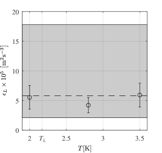
Figure 11: Dissipation rate $\epsilon_{L}$ for the three explored temperatures computed using the $\sigma_{u}$ obtained from ballistic separation method. The gray area shows the range of expected values for $\epsilon$ according to empirical laws.

Fig. 11, shows the estimates of $\epsilon_{L}$ for the three different experimental configurations we have explored. The gray area in fig. 11 depicts the range of expected values for $\epsilon$ in our experimental conditions, considering the main uncertainty which lies in the value of experimental constants as determined by earlier studies $c_{u}=0.25\pm 0.025$ and $c_{L}=0.2\pm 0.05$, [5, 29, 40, 38, 7]. Furthermore, the experimental area is located at $z=4.6\pm 0.6M$ distance from the grid, and $\epsilon$ is expected to scale as $z^{-2}$.

We find that within experimental error bars, the estimates of $\epsilon_{L}$ are in good agreement, with empirical laws for classical turbulence at large scales. Besides, no significant difference is observed between He I and He II.

VII.2 Estimate of energy transfer at Inertial scales

Assuming classical homogeneous isotropic turbulent scalings, the energy transfer rate $\epsilon_{I}$ through the inertial scales is classically estimated from the Eulerian second-order structure function ($S_{2}^{E}(r)=\frac{11}{3}C_{2}(\epsilon_{I}~{}r)^{\frac{2}{3}}$), which in a Lagrangian prospect, can robustly be calculated from particles relative dispersion statistics [3]. As described below, this method has the benefit to give an estimate of the structure function based on position increments, without requiring the calculation of particles velocities. This way we avoid having to differentiate trajectories individually, which as discussed previously is very sensitive to experimental noise.

VII.2.1 Methodology - Estimate of Eulerian $S_{2}^{E}$ from pair separation statistics

The second order Eulerian structure function can be efficiently estimated from displacement statistics by considering pair statistics. Particle pair dispersion was first introduced in 1926 by Richardson [24] and has become since a classical problem of Lagrangian turbulence. We will only be interested here in the short time separation regime (also called ballistic regime  [3]), which is the relevant regime to estimate $S_{2}^{E}$. Consider two particles with an initial separation $\vec{D}_{0}$, the quadratic relative separation between two particles can be written

$$R_{D_{0}}^{2}(t)=\langle|\vec{D}(t)~{}-~{}\vec{D}_{0}|^{2}\rangle,$$

with $D(t)$ the instantaneous separation between the particles, and where the average $\langle\cdot\rangle$ is taken over a set of particles with identical initial separation $\left|D_{0}\right|$. By a simple Taylor expansion, one can show that in the limit $t\rightarrow 0$ (ballistic regime) $R_{D_{0}}^{2}$ is kinematically related to $S_{2}^{E}$ by:

$$R_{D_{0}}^{2}(t)=S_{2}^{E}(D_{0})t^{2}+\mathcal{O}(t^{3}).$$ (12)

By fitting a quadratic relation for the early stage pair separation while sweeping the value of initial separation $D_{0}$, it is therefore possible to infer $S_{2}^{E}(r)$ across scales. Compared to a direct estimate from the velocity increments, this method to estimate $S_{2}^{E}$ has the great benefit to avoid computing position derivative, thus limiting the amplification of experimental noise.

Note that in practice, we will only consider the relative quadratic separation $R_{D_{0},x}^{2}(t)$ in the $x$ direction, so that the above mentioned procedure will give access to the one-component structure function $S_{2,x}^{E}(r)$. In isotropic conditions $S_{2,x}^{E}(r)$ is simply one third of the total structure function $S_{2}^{E}(r)$).

Finally, assuming classical Kolmogorov scalings for $S_{2}^{E}$, one can then estimate $\epsilon$ from $R_{D_{0},x}^{2}(t)$ using the relation (only valid in the limit of small time lags):

$$\frac{R_{D_{0},x}^{2}(t)}{\frac{11}{9}C_{2}D_{0}^{2/3}}=\epsilon_{I}^{2/3}t^{2}+{\mathcal{O}}(t^{3}).$$ (13)

VII.2.2 Results

Fig. 12 presents the time evolution of the normalized mean square separation (we only consider the separation in $x$ direction) $\frac{R_{D_{0},x}^{2}}{\frac{11}{9}C_{2}D_{0}^{2/3}}$ against $t$. Each curve is for a specific bin of initial separation $D_{0}$. The expected ballistic regime is clearly visible for time lags $t\approx\tau_{\eta}$. A deviation from the ballistic regime can be seen at the shortest time lags. This is a signature of the noise in the position measurement: in the limit of a purely random (Brownian like noise) the particle separation rate is expected to be purely diffusive ($R^{2}(t)\propto t$), which is consistent with the less steep slope at short times.

By individually fitting each curve in fig. 12 against $t^{2}$, we can extract the value of the slope $\alpha(D_{0})=S^{E}_{2,x}/\frac{11}{9}C_{2}D_{0}^{2/3}$ for each initial separation $D_{0}$. Assuming Kolmogorov scaling, we can then assess $\epsilon_{I}$ using the relation $\epsilon_{I}=\alpha(D_{0})^{3/2}$ (see eq 13). The result of this fitting procedure is shown in fig. 13 as a function of the initial separation $D_{0}$.

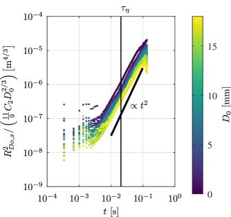
Figure 12: Time evolution of $\frac{R_{D_{0},x}^{2}}{\frac{11}{9}C_{2}D_{0}^{2/3}}$ in config. 3 (He I).

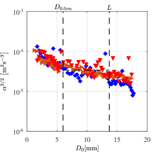
Figure 13: Coefficient $\alpha^{3/2}$ against the initial separation $D_{0}$, where $\alpha$ is defined as $\frac{R_{D_{0},x}^{2}}{\frac{11}{9}C_{2}D_{0}^{2/3}}=\alpha t^{2}+\beta$. $\blacktriangledown$ config. 1, $\blacktriangleright$ config. 2, $\blacklozenge$ config. 3.

A first important interesting finding is that fig. 13 does not highlight any measurable difference between He I and He II situations. We see a pseudo-plateau in the inertial range (we recall that in the present situation the integral scale is estimated to be $L\simeq 14$ mm), indicating a reasonable Kolmogorov scaling. At small scales, one would expect a trivial dissipative scaling $S_{2}(D_{0})\propto D_{0}^{2}$, and hence $\alpha\propto S_{2}/D_{0}^{2/3}\propto D_{0}^{4/3}$, what is clearly inconsistent with the rapid increase observed in fig. 13 as $D_{0}$ decreases below $D_{0}\sim 5$  mm. This is primarily due to the fact that small scales are biased by the finite depth of field ($\delta_{dof}\simeq 1.4$ mm) of our measurement volume, since we only have access to 2D measurements. Estimate of separation data are therefore accurate only in the limit $D_{0}>\delta_{dof}$. Besides, given the dilute nature of our flow there is not enough statistics at small $D_{0}$. For separations $D_{0}$ of order and smaller than $\delta_{dof}$, the possible overlap of the 2D projection of particles within the depth of field, allows for large relative velocities even in the limit of small apparent separations.

We therefore estimate the dissipation rate $\epsilon_{I}$, by averaging $\alpha^{3/2}$ over the pseudo-plateau in the range 6 mm$<D_{0}<$ 14 mm, corresponding to inertial scales not significantly affected by the finite depth of field bias. This corresponds to the two vertical dashed lines represented in fig. 13.

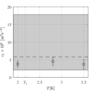
Figure 14: Dissipation rate $\epsilon_{I}$ for the three explored temperatures computed the second order structure function estimated from pair separation. The gray area shows the range of expected values for $\epsilon$ according to empirical laws.

The corresponding values of $\epsilon_{I}$ as a function of the operating temperature is shown in fig. 14. It is found that, within error bars, the inertial scale estimate $\epsilon_{I}$ is in good agreement both with empirical laws and with the large scale estimate $\epsilon_{L}$ discussed in the previous section. In particular, no difference is observed between HeII and HeI.

VII.3 Dissipative scales

Estimation of the dissipation at dissipative scales requires the analysis of small scale information. In the Eulerian context, this usually drives back to the definition of dissipation $\epsilon_{\eta}=2\nu\Omega^{2}$ (with $\Omega^{2}$ the enstrophy), which in homogeneous isotropic turbulence can simply be rewritten in terms of a single component (say $u$) spatial derivative : $\epsilon_{\eta}=15\nu\partial_{x}u$. This requires measurements with high spatial resolution, allowing to take well resolved spatial derivative of the velocity field. In the context of Lagrangian measurements, as in the present study, the relevant small scale quantity is the Lagrangian acceleration (rather than the velocity gradient), which is related to the dissipation rate via the Heisenberg-Yaglom relation:

$$\sigma_{ax}^{2}~{}=a_{0}\epsilon_{\eta}^{3/2}\nu^{-1/2}.$$ (14)

In this relation $\sigma_{ax}$ is the standard deviation of horizontal acceleration fluctuations and $a_{0}$ is a dimensionless coefficient that is empirically known in classical turbulence (from experimental and numerical studies, see for instance the review article of Toschi and Bodenschatz [39]) and which is known to depend on the Reynolds number following an empirical law $a_{0}\simeq 0.85R_{\lambda}^{-.25}$, see [43].

Unfortunately, considering the noise issues previously discussed regarding the direct estimates of velocity statistics, it is unlikely that our measurements are sufficiently well resolved at small temporal scales to actually resolve second order Lagrangian derivatives required to estimate acceleration, as taking second order derivatives is extremely sensitive to experimental noise.

Still we attempted to perform this estimate. The acceleration is calculated by convolution of particles trajectories with a second derivative gaussian kernel, as classically done in Lagrangian studies to estimate filtered derivatives [16], with the same filtering parameters (in particular the same filter width as for the direct velocity estimates previously discussed in section  VI). From this data we calculate the acceleration variance $\sigma_{a_{x}}$ which is then used to estimate the small scale dissipation rate from the Heisenberg-Yaglom relation. The corresponding results are plotted as a function of the operating temperature in fig.15.

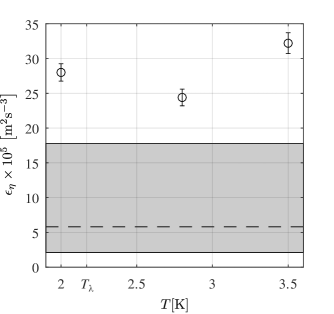
Figure 15: Dissipation rate $\epsilon_{\eta}$ vs Temperature $T$ at dissipative scales.

As one can see on fig. 15, our experimental data do not match the expected values from literature, neither in He I nor in He II. Consequently, this result cannot be attributed to a particular behavior of HeII but rather to an insufficient temporal resolution to accurately estimate the acceleration at dissipative scales. Efforts are been put at present on the experimental side in order to improve this and perform new measurements with sufficient resolution at inertial and dissipative scales.

VIII Conclusion

Our experiment has been calibrated and validated against canonical oscillating grid turbulence in classical flows. Indeed, our results in He I match empirical data.

We did not find any difference in preferential concentration once HeII was used. This may be due to the relatively large particle size that we used (85 $\mu$m) which prevent particles from getting trapped by superfluid vortex lines. Another possibility is that in isothermal HeII flow, at sufficiently high Re, the superfluid component is really linked to the normal one as it has been recently reported that superfluid component mimics the normal flow, for both large velocity field and vorticity, see [26].

We noticed the existence of a mean drift of the particles in the z-direction with a slight impact on the measured fluctuating velocity in the z-direction. So for the assessment of the dissipation rate we focused on the horizontal components. At large and inertial scales results in He I are as expected in classical fluids. Furthermore, in these range of currently accessible scales, our study does not reveal any difference of turbulence properties between He I and He II. This may be explained by the fact that quite large particles (diameter of 85$\mu$m) are used and at 2K there is only 39% of inviscid component in the superfluid. Indeed the effect of quantum turbulence is expected to appear below a scale where normal and superfluid component are decoupled (e.g. below the inter vortex distance). Unfortunately, whilst the spatial and temporal resolution of our measurements give us access to the dynamics of the flow in the range of inertial scales, dissipative scales are marginally resolved.

Further studies aim at achieving even higher resolution measurements to explore possible differences between classical and superfluid turbulence at and below dissipative scales. To do so, either smaller particles (while keeping spherical shape and monodisperse size) or lower Re number (while remaining fully turbulent) or larger facility should be used.

References

- Babuin et al. [2014] Simone Babuin, Emil Varga, Ladislav Skrbek, Emmanuel Lévêque, and Philippe-E. Roche. Effective viscosity in quantum turbulence: A steady-state approach. EPL (Europhysics Letters), 106(2):24006, apr 2014. doi: 10.1209/0295-5075/106/24006. URL https://doi.org/10.1209%2F0295-5075%2F106%2F24006.
- Bewley et al. [2008] G. P. Bewley, M. Paoletti, D. P. Lathrop, and K. R. Sreenivasan. Visualization of quantize vortex dynamics. In IUTAM Symposium on computational physics and new perspectives in turbulence, volume 4 of IUTAM Bookseries, pages 163–170, 2008.
- Bourgoin [2015] M. Bourgoin. Turbulent pair dispersion as a ballistic cascade phenomenology. J. Fluid Mech., 2015.
- Chopra and Brown [1957] K. L. Chopra and J. B. Brown. Suspension of particles in liquid helium. Phys. Rev., 108:157–157, 1957.
- Eidelman et al. [2001] A. Eidelman, T. Elperin, A. Kapusta, N. Kleeorin, A. Krein, and I. Rogachevskii. Oscillating grids turbulence generator for turbulent transport studies. Nonlinear Processes in Geophysics, pages 201–205, 2001.
- Fernando and I.P [1993] H. J. S. Fernando and D. De Silva I.P. Note on secondary flows in oscillating grid, mixingbox experiments. Physics of Fluids A, 5:1849, July 1993.
- Hopfinger and Toly [1976] E. J. Hopfinger and J.-A. Toly. Spatially decaying turbulence and its relation to mixing across density interfaces. J. Fluid Mech., 78:155–175, January 1976.
- Kitchens et al. [1965] T. A. Kitchens, W. A. Steyert, R. D. Taylor, and Paul P. Craig. Flow visualization in he ii: Direct observation of helmholtz flow. Phys. Rev. Lett., 14:942–945, 1965.
- Klein et al. [2013] Simon Klein, Mathieu Gibert, Antoine Bérut, and Eberhard Bodenschatz. Simultaneous 3D measurement of the translation and rotation of finite-size particles and the flow field in a fully developed turbulent water flow. Measurement Science and Technology, 2013. ISSN 13616501. doi: 10.1088/0957-0233/24/2/024006.
- Mantia et al. [2012] M. La Mantia, T. V. Chagovets, M. Rotter, and L. Skrbek. Testing the performance of a cryogenic visualization system on thermal counterflow by using hydrogen and deuterium solid tracers. RSI, 83, May 2012.
- Mantia [2016] Marco La Mantia. Particle trajectories in thermal counterflow of superfluid helium in a wide channel of square cross section. Physics of Fluids, 28, 2016.
- Mastracci and Guo [2018] Brian Mastracci and Wei Guo. Exploration of thermal counterflow in he ii using particle tracking velocimetry. Physical Review Fluids, 3(6):063304, 2018.
- Maurer and Tabeling [1998] J. Maurer and P. Tabeling. Local investigation of superfluid turbulence. Europhysics Letters, 43(1):29–34, 1998.
- McKenna and McGillis [2004] S. P. McKenna and W. R. McGillis. Observations of flow repeatability and secondary circulation in an oscillating grid-stirred tank. Physics of Fluids, 16(9), August 2004.
- Monchaux [2012] R. Monchaux. Measuring concentration with voronoï diagrams : the study of possible biases. New Journal of Physics, 2012.
- Mordant et al. [2004a] N. Mordant, A. M. Crawford, and E Bodenschatz. Experimental lagrangian acceleration probability density function measurement. Physica D, 193:245–251, 2004a.
- Mordant et al. [2004b] Nicolas Mordant, Alice M Crawford, and Eberhard Bodenschatz. Three-dimensional structure of the lagrangian acceleration in turbulent flows. Physical Review Letters, 93(21):214501, 2004b. URL http://prl.aps.org/abstract/PRL/v93/i21/e214501.
- Murakami and Ichikawa [1989a] M. Murakami and N. Ichikawa. Flow visualisation study of thermal counterflow jet in heii. Cryogenics, 29, 1989a.
- Murakami and Ichikawa [1989b] M Murakami and N Ichikawa. Flow visualization study of thermal counterflow jet in he ii. Cryogenics, 29(4):438–443, 1989b.
- Ouellette et al. [2006] N. Ouellette, H. xu, M. Bourgoin, and E. Bodenschatz. An experimental study of turbulent relative dispersion models. New Journal of Physics, 2006.
- Ouellette [2011] Nicholas T. Ouellette. Particle tracking. https://web.stanford.edu/~nto/software_tracking.shtml, 2011. [Online; accessed 01-June-2020].
- Paoletti et al. [2008] M. S. Paoletti, R. B. Fiorito, K. R. Sreenivasan, and D. P. Lathrop. Visualization of superfluid helium flow. Journal of the Phydical Society of Japan, 77(11), 2008.
- PNAS [2013] PNAS, editor. Visualisation of two-fluid flows of superfluid helium-4, 2013.
- Richardson [1926] Lewis F. Richardson. Atmospheric diffusion shown on a distance-neighbour graph. Proceedings of the Royal Society of London. Series A. Mathematical and Physical Sciences, 10(756):709–737, 1926. doi: 10.1098/rspa.1926.0043.
- Rousset et al. [2001] B. Rousset, D. Chatain, D. Beysens, and B. Jager. Two-phase visualization at cryogenic temperature. Cryogenics, 41:443–451, 2001.
- Rusaouen et al. [2017] E. Rusaouen, B. Rousset, and P.-E. Roche. Detection of vortex coherent structures in superfluid turbulence. EPL (Europhysics Letters), 118, June 2017.
- Salort et al. [2010] Julien Salort, Christophe Baudet, Bernard Castaing, Benoît Chabaud, François Daviaud, Thomas Didelot, Pantxo Diribarne, Bérengère Dubrulle, Yves Gagne, Frédéric Gauthier, et al. Turbulent velocity spectra in superfluid flows. Physics of Fluids, 22(12):125102, 2010.
- Silva and Fernando [1992] I. P. D. De Silva and H. J. S. Fernando. Some aspects of mixing in a stratified turbulent patch. Journal of Fluid Mechanics, 240:601 – 625, January 1992.
- Silva and Fernando [1994] I. P. D. De Silva and H. J. S. Fernando. Oscillating grids as a source of nearly isotropic turbulence. Physics of Fluids, 6(7):2455, July 1994.
- Skrbek [2006] L. Skrbek. Energy spectra of quantum turbulence in heii and 3he-b : A unifief view. JETP Letters, 83(3):127–131, 2006.
- Sreenivasan [1984] K. R. Sreenivasan. On the scaling of the turbulence energy dissipation rate. Physics of Fluids, 27(5):1048–1050, 1984.
- Sreenivasan [1998] Katepalli R. Sreenivasan. An update on the energy dissipation rate in isotropic turbulence. Physics of Fluids, 10(2):528–529, 1998. doi: 10.1063/1.869575.
- Stalp et al. [1999] Steven R Stalp, L Skrbek, and Russell J Donnelly. Decay of grid turbulence in a finite channel. Physical review letters, 82(24):4831, 1999.
- Svancara and La Mantia [2017] P. Svancara and M. La Mantia. Flows of liquid 4he due to oscillating grids. J. Fluid Mech., 832:578–599, 2017.
- Sy et al. [2015] N. F. Sy, M. Bourgoin, P. Diribarne, M. Gibert, and B. Rousset. Oscillating grid high reynolds experiments in superfluid. In Proc. 15th European Turbulence Conference, number 318, 2015.
- T Ouellette et al. [2006] Nicholas T Ouellette, Haitao Xu, Mickael Bourgoin, and Eberhard Bodenschatz. Small-scale anisotropy in lagrangian turbulence. New Journal of Physics, 8, 06 2006.
- Tang et al. [2020] Yuan Tang, Shiran Bao, Toshiaki Kanai, and Wei Guo. Statistical properties of homogeneous and isotropic turbulence in he ii measured via particle tracking velocimetry. Physical Review Fluids, 5(8):084602, 2020.
- Thompson and Turner [1975] S.M. Thompson and J.S. Turner. Mixing across an interface due to turbulence generated by an oscillating grid. Journal of Fluid Mechanics, 67, January 1975.
- Toschi and Bodenschatz [2009] Federico Toschi and Eberhard Bodenschatz. Lagrangian properties of particles in turbulence. Annual Review of Fluid Mechanics, 41(1):375–404, 2009. doi: 10.1146/annurev.fluid.010908.165210.
- Villermaux et al. [1995] E. Villermaux, B. Sixou, and Y. Gagne. Intense vortical structures in grid generated turbulence. Physics of Fluids, 1995.
- Vinen and Niemela [2002] W. F. Vinen and J. J. Niemela. Quantum turbulence. Journal of Low Temperature Physics., 128, September 2002.
- Vinen and Shoenberg [1957] William Frank Vinen and David Shoenberg. Mutual friction in a heat current in liquid helium ii iii. theory of the mutual friction. Proceedings of the Royal Society of London. Series A. Mathematical and Physical Sciences, 242(1231):493–515, 1957. doi: 10.1098/rspa.1957.0191.
- Voth et al. [2002] G. A. Voth, A. La Porta, A. M. Crawford, J. Alexander, and E. Bodenschatz. Measurement of lagrangian velocity in fully developed turbulence. J. Fluid Mechanics, 469:121–160, 2002.
- White et al. [2002] C. M. White, A. N. Karpetis, and K. R. Sreenivasan. High-reynolds number turbulence in small apparatus: grid turbulence in cryogenic liquids. J. Fluid Mech., 452:189–197, 2002.
- Williams and Packard [1974] Gary A. Williams and Richard E. Packard. Photographs of quantized vortex lines in rotating he ii. Phys. Rev. Lett., 33:280–283, 1974.