LiDAR-based Panoptic Segmentation via Dynamic Shifting Network

Abstract

With the rapid advances of autonomous driving, it becomes critical to equip its sensing system with more holistic 3D perception. However, existing works focus on parsing either the objects (cars and pedestrians) or scenes (trees and buildings) from the LiDAR sensor. In this work, we address the task of LiDAR-based panoptic segmentation, which aims to parse both objects and scenes in a unified manner. As one of the first endeavors towards this new challenging task, we propose the Dynamic Shifting Network (DS-Net), which serves as an effective panoptic segmentation framework in the point cloud realm. In particular, DS-Net has three appealing properties: 1) strong backbone design. DS-Net adopts the cylinder convolution that is specifically designed for LiDAR point clouds. The extracted features are shared by the semantic branch and the instance branch which operates in a bottom-up clustering style. 2) Dynamic Shifting for complex point distributions. We observe that commonly-used clustering algorithms like BFS or DBSCAN are incapable of handling complex autonomous driving scenes with non-uniform point cloud distributions and varying instance sizes. Thus, we present an efficient learnable clustering module, dynamic shifting, which adapts kernel functions on-the-fly for different instances. 3) Consensus-driven Fusion. Finally, consensus-driven fusion is used to deal with the disagreement between semantic and instance predictions. To comprehensively evaluate the performance of LiDAR-based panoptic segmentation, we construct and curate benchmarks from two large-scale autonomous driving LiDAR datasets, SemanticKITTI and nuScenes. Extensive experiments demonstrate that our proposed DS-Net achieves superior accuracies over current state-of-the-art methods. Notably, we achieve 1st place on the public leaderboard of SemanticKITTI, outperforming 2nd place by 2.6% in terms of the PQ metric .

1 Introduction

Autonomous driving, one of the most promising applications of computer vision, has achieved rapid progress in recent years. Perception system, one of the most important modules in autonomous driving, has also attracted extensive studies in previous research works. Admittedly, the classic tasks of 3D object detection [18, 24, 32] and semantic segmentation [20, 30, 35] have developed relatively mature solutions that support real-world autonomous driving prototypes. However, there still exists a considerable gap between the existing works and the goal of holistic perception which is essential for the challenging autonomous driving scenes. In this work, we propose to close the gap by exploring the task of LiDAR-based panoptic segmentation, which requires full-spectrum point-level predictions.

Panoptic segmentation has been proposed in 2D detection [15] as a new vision task which unifies semantic and instance segmentation. Behley et al.[3] extend the task to LiDAR point clouds and propose the task of LiDAR-based panoptic segmentation. As shown in Fig. 1 (a), this task requires to predict point-level semantic labels for background (stuff) classes (road, building and vegetation), while instance segmentation needs to be performed for foreground (things) classes (car, person and cyclist).

Nevertheless, the complex point distributions of LiDAR data make it difficult to perform reliable panoptic segmentation. Most existing point cloud instance segmentation methods [10, 14] are mainly designed for dense and uniform indoor point clouds. Therefore, decent segmentation results can be achieved through the center regression and heuristic clustering algorithms. However, due to the non-uniform density of LiDAR point clouds and varying sizes of instances, the center regression fails to provide ideal point distributions for clustering. The regressed centers usually form noisy strip distributions that vary in density and sizes. As will be analyzed in Section 3.2, several heuristic clustering algorithms widely used in previous works cannot provide satisfactory clustering results for the regressed centers of LiDAR point clouds. To tackle the above mentioned technical challenges, we propose Dynamic Shifting Network (DS-Net) which is specifically designed for effective panoptic segmentation of LiDAR point clouds.

Firstly, we adopt a strong backbone design and provide a strong baseline for the new task. Inspired by [37], the cylinder convolution is used to efficiently extract grid-level features for each LiDAR frame in one pass which are further shared by the semantic and instance branches.

Secondly, we present a novel Dynamic Shifting Module designed to cluster on the regressed centers with complex distributions produced by the instance branch. As illustrated in Fig. 1 (b), the proposed dynamic shifting module shifts the regressed centers to the cluster centers. The shift targets $x_{i}$ are adaptively computed by weighting across several shift candidates $c_{ij}$ which are calculated through kernel functions $k_{j}$. The special design of the module makes the shift operation capable of dynamically adapting to the density or sizes of different instances and therefore shows superior performance on LiDAR point clouds. Further analysis also shows that the dynamic shifting module is robust and not sensitive to parameter settings.

Thirdly, the Consensus-driven Fusion Module is presented to unify the semantic and instance results to obtain panoptic segmentation results. The proposed consensus-driven fusion mainly solves the disagreement caused by the class-agnostic style of instance segmentation. The fusion module is highly efficient, thus brings negligible computation overhead.

Extensive experiments on SemanticKITTI demonstrate the effectiveness of our proposed DS-Net. To further illustrate the generalizability of DS-Net, we customize a LiDAR-based panoptic segmentation dataset based on nuScenes. As one of the first works for this new task, we present several strong baseline results by combining the state-of-the-art semantic segmentation and detection methods. DS-Net outperforms all the state-of-the-art methods on both benchmarks (1st place on the public leaderboard of SemanticKITTI).

The main contributions are summarized below: 1) To our best knowledge, we present one of the first attempts to address the challenging task of LiDAR-based panoptic segmentation. 2) The proposed DS-Net effectively handles the complex distributions of LiDAR point clouds, and achieves state-of-the-art performance on SemanticKITTI and nuScenes. 3) Extensive experiments are performed on large-scale datasets. We adapt existing methods to this new task for in-depth comparisons. Further statistical analyses are carried out to provide valuable observations.

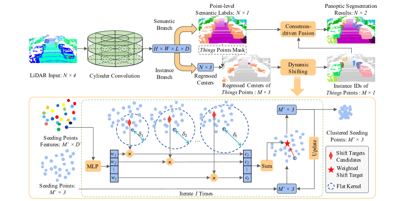
Figure 2: Architecture of the DS-Net. The DS-Net consists of the cylinder convolution, a semantic and an instance branch as shown in the upper part of the figure. The regressed centers provided by the instance branch are clustered by the novel dynamic shifting module which is shown in the bottom half. The consensus-driven fusion module unifies the semantic and instance results into the final panoptic segmentation results.

2 Related Works

Point Cloud Semantic Segmentation. According to the data representations of point clouds, most point cloud semantic segmentation methods can be categorized to point-based and voxel-based methods. Based on PointNet [22] and PointNet++ [23], KPConv [25], DGCNN [28], PointConv [31] and Randla-Net [13] can directly operate on unordered point clouds. However, due to space and time complexity, most point-based methods struggle on large-scale point clouds datasets ScanNet [9], S3DIS [1], and SemanticKITTI [2]. MinkowskiNet [7] utilizes the sparse convolutions to efficiently perform semantic segmentation on the voxelized large-scale point clouds. Different from indoor RGB-D reconstruct point clouds, LiDAR point clouds have non-uniform and sparse point distributions which require special designs of the network. SqueezeSeg [30] views LiDAR point clouds as range images while PolarNet [35] and Cylinder3D [37] divide the LiDAR point clouds under the polar and cylindrical coordinate systems. Compared to other data representations, cylindrical division is more suitable for sparse and non-uniform LiDAR point clouds because it fully utilizes the localization of point clouds while remains high efficiency.

Point Cloud Instance Segmentation. Previous works have shown great progress in the instance segmentation of indoor point clouds. A large number of point-based methods (SGPN [26], ASIS [27], JSIS3D [21] and JSNet [36]) split the whole scene into small blocks and learn point-wise embeddings for final clustering. Although great efforts have been made on semantic and instance branch merging in order to boost each other’s performance, these methods are limited by the heuristic post processing steps and the lack of perception. To avoid the problems, recent works (PointGroup [14], 3D-MPA [10], OccuSeg [12]) abandon the block partition and use sparse convolutions to extract features of the whole scene in one pass. As for LiDAR point clouds, there are a few previous works [13, 29, 30, 34] trying to tackle the problem. Wu et al.[30] directly cluster on XYZ coordinates after semantic segmentation. Wong et al.[29] builds the network in a top-down style and incorporates metric learning. Zhang et al.[34] uses grid-level center voting to cluster points of interest in autonomous driving scenes. Although our work is not targeting the instance segmentation for LiDAR point clouds, the proposed DS-Net can provide some insights into the challenging task.

3 Our Approach

As one of the first attempts on the task of LiDAR-based panoptic segmentation, we first introduce a strong backbone to establish a simple baseline (Sec. 3.1), based on which two modules are further proposed. The novel dynamic shifting module is presented to tackle the challenge of the non-uniform LiDAR point clouds distributions (Sec. 3.2). The efficient consensus-driven fusion module combines the semantic and instance predictions and produces panoptic segmentation results (Sec. 3.3). The whole pipeline of the DS-Net is illustrated in Fig. 2.

3.1 Strong Backbone Design

To obtain panoptic segmentation results, it is natural to solve two sub-tasks separately, which are semantic and instance segmentation, and combine the results. As shown in the upper part of Fig. 2, the strong backbone consists of three parts: the cylinder convolution, a semantic branch, and an instance branch. High quality grid-level features are extracted by the cylinder convolution from raw LiDAR point clouds and then shared by semantic and instance branches.

Cylinder Convolution. Considering the difficulty presented by the task, we find that the cylinder convolution [37] best meets the strict requirements of high efficiency, high performance and fully mining of 3D positional relationship. The cylindrical voxel partition can produce more even point distribution than normal Cartesian voxel partition and therefore leads to higher feature extraction efficiency and higher performance. Cylindrical voxel representation combined with sparse convolutions can naturally retain and fully explore 3D positional relationship. Thus we choose the cylinder convolution as our feature extractor.

Semantic Branch. The semantic branch performs semantic segmentation by connecting MLP to the cylinder convolution to predict semantic confidences for each voxel grid. Then the point-wise semantic labels are copied from their corresponding grids. We use the weighted cross entropy and Lovasz Loss [4] as the loss function of the semantic branch.

Instance Branch. The instance branch utilizes center regression to prepare the things points for further clustering. The center regression module uses MLP to adapt cylinder convolution features and make things points to regress the centers of their instances by predicting the offset vectors $O\in\mathbb{R}^{M\times 3}$ pointing from the points $P\in\mathbb{R}^{M\times 3}$ to the instance centers $C_{gt}\in\mathbb{R}^{M\times 3}$. The loss function for instance branch can be formulated as:

$$L_{ins}=\frac{1}{M}\sum_{i=0}^{M}\lVert O[i]-(C_{gt}[i]-P[i])\rVert_{1}\text{,}$$ (1)

where $M$ is the number of things points. The regressed centers $O+P$ are further clustered to obtain the instance IDs, which can be achieved by either heuristic clustering algorithms or the proposed dynamic shifting module which are further introduced and analyzed in the following section.

3.2 Dynamic Shifting

Point Clustering Revisit. Unlike indoor point clouds which are carefully reconstructed using RGB-D videos, the LiDAR point clouds have the distributions that are not suitable for normal clustering solutions used by indoor instance segmentation methods. The varying instance sizes, the sparsity and incompleteness of LiDAR point clouds make it difficult for the center regression module to predict the precise center location and would result in noisy long strips distribution as displayed in Fig. 1 (b) instead of an ideal ball-shaped cluster around the center. Moreover, as presented in Fig. 3 (a), the clusters formed by regressed centers that are far from the LiDAR sensor have much lower densities than those of nearby clusters due to the non-consistent sparsity of LiDAR point clouds. Facing the non-uniform distribution of regressed centers, heuristic clustering algorithms struggle to produce satisfactory results. Four major heuristic clustering algorithms that are used in previous bottom-up indoor point clouds instance segmentation methods are analyzed below. The details of the following algorithms can be found in supplementary materials.

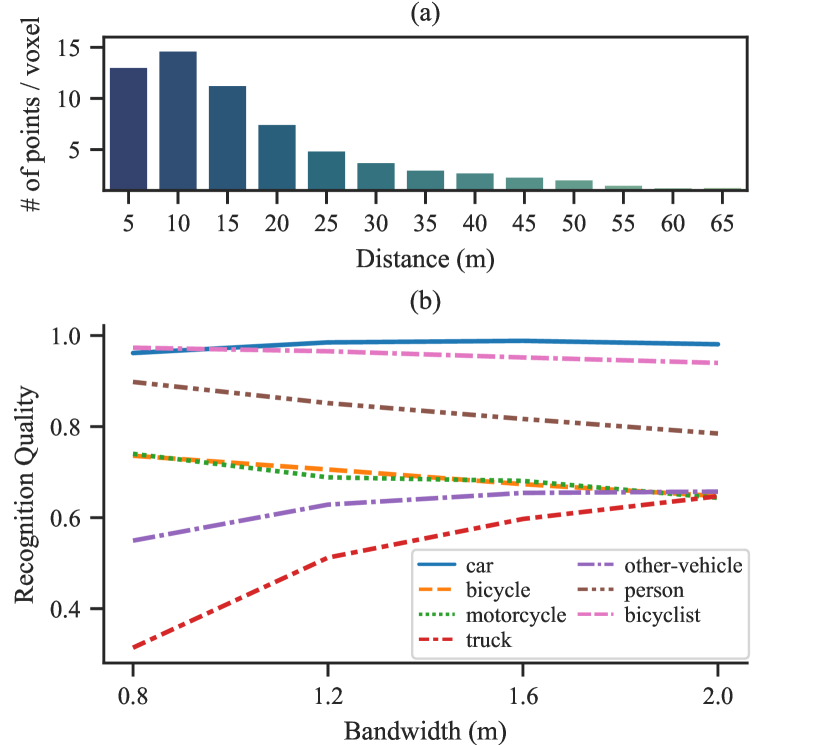
Figure 3: (a) counts the average number of regressed centers inside each valid voxel of instances at different distances. (b) shows the effect of Different Mean Shift Bandwidth on the Recognition Quality of Different Classes.

• Breadth First Search (BFS). BFS is simple and good enough for indoor point clouds as proved in [14], but not suitable for LiDAR point clouds. As discussed above, large density difference between clusters means that the fixed radius cannot properly adapt to different clusters. Small radius will over-segment distant instances while large radius will under-segment near instances.

• DBSCAN [11] and HDBSCAN [6]. As density-based clustering algorithms, there is no surprise that these two algorithms also perform badly on the LiDAR point clouds, even though they are proved to be effective for clustering indoor point clouds [10, 33]. The core operation of DBSCAN is the same as that of BFS. While HDBSCAN intuitively assumes that the points with lower density are more likely to be noise points which is not the case in LiDAR points.

• Mean Shift [8]. The advantage of Mean Shift, which is used by [17] to cluster indoor point clouds, is that the kernel function is not sensitive to density changes and robust to noise points which makes it more suitable than density-based algorithms. However, the bandwidth of the kernel function has great impact on the clustering results as shown in Fig. 3 (b). The fixed bandwidth cannot handle the situation of large and small instances simultaneously which makes Mean Shift also not the ideal choice for this task.

Input: Things Points $P\in\mathbb{R}^{M\times 3}$, Things Features $F\in\mathbb{R}^{M\times D^{\prime}}$, Things Regressed Centers $C\in\mathbb{R}^{M\times 3}$, Fixed number of iteration $I\in\mathbb{N}$, Bandwidth candidates list $L\in\mathbb{R}^{l}$

Output: Instance IDs of things points $R\in\mathbb{R}^{M\times 1}$

1 $mask=FPS(P)$, $P^{\prime}=P[mask]$

2 $X=C[mask]$, $F^{\prime}=F[mask]$

3 for $i\leftarrow 1\ \textnormal{{to}}\ I$ do

4       $W_{i}=Softmax(MLP(F^{\prime}))$

5       $acc=zeros\_like(X)$

6       for $j\leftarrow 1\ \textnormal{{to}}\ l$ do

7             $K_{ij}=(XX^{T}\leq L[j])$

8             $D_{ij}=diag(K_{ij}\mathbf{1})$

9             $acc=acc+W_{i}[:,j]\odot(D_{ij}^{-1}K_{ij}X)$

10       end for

11      $X=acc$

12      

13 end for

14 $R^{\prime}=cluster(X)$

15 $index=nearest\_neighbour(P,P^{\prime})$

16 $R=R^{\prime}[index]$

return $R$

Algorithm 1 Forward Pass of the Dynamic Shifting Module

Dynamic Shifting. As discussed above, it is a robust way of estimating cluster centers of regressed centers by iteratively applying kernel functions as in Mean Shift. However, the fixed bandwidth of kernel functions fails to adapt to varying instance sizes. Therefore, we propose the dynamic shifting module which can automatically adapt the kernel function for each LiDAR point in the complex autonomous driving scene so that the regressed centers can be dynamically, efficiently and precisely shifted to the correct cluster centers.

In order to make the kernel function learnable, we first consider how to mathematically define a differentiable shift opration. Inspired by [16], the shift operation on the seeding points (points to be clustered) can be expressed as matrix operations if the number of iterations is fixed. Specifically, one iteration of shift operation can be formulated as follows. Denoting $X\in\mathbb{R}^{M\times 3}$ as the $M$ seeding points, $X$ will be updated once by the shift vector $S\in\mathbb{R}^{M\times 3}$ which is formulated as

$$X\leftarrow X+\eta S\text{,}$$ (2)

where $\eta$ is a scaling factor which is set to $1$ in our experiments.

The calculation of the shift vector $S$ is by applying kernel function $f$ on $X$, and formally defined as $S=f(X)-X$.

Among various kinds of kernel functions, the flat kernel is simple but effective for generating shift target estimations for LiDAR points, which is introduced as follows. The process of applying flat kernel can be thought of as placing a query ball of certain radius (bandwidth) centered at each seeding point and the result of the flat kernel is the mass of the points inside the query ball. Mathematically, the flat kernel $f(X)=D^{-1}KX$ is defined by the kernel matrix $K=(XX^{T}\leq\delta)$, which masks out the points within a certain bandwidth $\delta$ for each seeding point, and the diagonal matrix $D=diag(K\mathbf{1})$ that represents the number of points within the seeding point’s bandwidth.

With a differentiable version of the shift operation defined, we proceed to our goal of dynamic shifting by adapting the kernel function for each point. In order to make the kernel function adaptable for instances with different sizes, the optimal bandwidth for each seeding point has to be inferenced dynamically. A natural solution is to directly regress bandwidth for each seeding point, which however is not differentiable if used with the flat kernel. Even though Gaussian kernel can make direct bandwidth regression trainable, it is still not the best solution as analyzed in section 4.1. Therefore, we apply the design of weighting across several bandwidth candidates to dynamically adapt to the optimal one.

One iteration of dynamic shifting is formally defined as follows. As shown in the bottom half of Fig. 2, $l$ bandwidth candidates $L=\{\delta_{1},\delta_{2},...,\delta_{l}\}$ are set. For each seeding point, $l$ shift target candidates are calculated by $l$ flat kernels with corresponding bandwidth candidates. Seeding points then dynamically decide the final shift targets, which are ideally the closest to the cluster centers, by learning the weights $W\in\mathbb{R}^{M\times l}$ to weight on $l$ candidate targets. The weights $W$ are learned by applying MLP and Softmax on the backbone features so that $\sum_{j=1}^{l}W[:,j]=\textbf{1}$. The above procedure and the new learnable kernel function $\hat{f}$ can be formulated as

$$\hat{f}(X)=\sum_{j=1}^{l}W[:,j]\odot(D_{j}^{-1}K_{j}X)\text{,}$$ (3)

where $K_{j}=(XX^{T}\leq\delta_{j})$ and $D_{j}=diag(K_{j}\mathbf{1})$.

With the one iteration of dynamic shifting stated clearly, the full pipeline of the dynamic shifting module, which is formally defined in algorithm 1, can be illustrated as follows. Firstly, to maintain the efficiency of the algorithm, farthest point sampling (FPS) is performed on $M$ things points to provide $M^{\prime}$ seeding points for the dynamic shifting iterations (Lines 1–1). After a fixed number $I$ of dynamic shifting iterations (Lines 1–1), all seeding points have converged to the cluster centers. A simple heuristic clustering algorithm is performed to cluster the converged seeding points to obtain instance IDs for each seeding point (Line 1). Finally, all other things points find the nearest seeding points and the corresponding instance IDs are assigned to them (Lines 1–1).

The optimization of dynamic shifting module is not intuitive since it is impractical to obtain the ground truth bandwidth for each seeding point. The loss function has to encourage seeding points shifting towards their cluster centers which have no ground truths but can be approximated by the ground truth centers of instances $C_{gt}^{\prime}\in\mathbb{R}^{M^{\prime}\times 3}$. Therefore, the loss function for the $i$th iteration of dynamic shifting is defined by the manhattan distance between the ground truth centers $C_{gt}^{\prime}$ and the $i$th dynamically calculated shift targets $X_{i}$, which can be formulated as

$$l_{i}=\frac{1}{M^{\prime}}\sum_{x=1}^{M^{\prime}}\lVert X_{i}[x]-C_{gt}^{\prime}[x]\rVert_{1}\text{.}$$ (4)

Adding up all the losses of $I$ iterations gives us the loss function $L_{ds}$ for the dynamic shifting module:

$$L_{ds}=\sum_{i=1}^{I}w_{i}l_{i}\text{,}$$ (5)

where $w_{i}$ are weights for losses of different iterations and are all set to $1$ in our experiments.

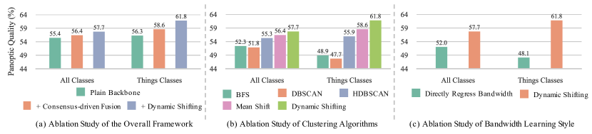
Figure 4: Ablation Study on the Validation Set of SemanticKITTI. The proposed two modules both contributes to the final performance of the DS-Net. The dynamic shifting module has advantages in clustering LiDAR point clouds. Weighting on bandwidth candidates is better than directly regressing bandwidth.

3.3 Consensus-driven Fusion

Typically, solving the conflict between semantic and instance predictions is one of the essential steps in panoptic segmentation. The advantages of bottom-up methods are that all points with predicted instance IDs must be in things classes and one point will not be assigned to two instances. The only conflict needs to be solved is the disagreement of semantic predictions inside one instance, which is brought in by the class-agnostic way of instance segmentation. The strategy used in the proposed consensus-driven fusion is majority voting. For each predicted instance, the most appeared semantic label of its points determines the semantic labels for all the points inside the instance. This simple fusion strategy is not only efficient but could also revise and unify semantic predictions using instance information.

4 Experiments

Table 1: LiDAR-based panoptic segmentation results on the validation set of SemanticKITTI. All results in [%].

Method	PQ	PQ$\dagger$	RQ	SQ	PQTh	RQTh	SQTh	PQSt	RQSt	SQSt	mIoU
KPConv [25] + PV-RCNN [24]	51.7	57.4	63.1	78.9	46.8	56.8	81.5	55.2	67.8	77.1	63.1
PointGroup [14]	46.1	54.0	56.6	74.6	47.7	55.9	73.8	45.0	57.1	75.1	55.7
LPASD [19]	36.5	46.1	-	-	-	28.2	-	-	-	-	50.7
DS-Net	57.7	63.4	68.0	77.6	61.8	68.8	78.2	54.8	67.3	77.1	63.5

Table 2: LiDAR-based panoptic segmentation results on the test set of SemanticKITTI. All results in [%]. “$\ast$” denotes the unpublished method which is in the 2nd place on the public benchmark of SemanticKITTI (accessed on 2020-11-16).

Method	PQ	PQ$\dagger$	RQ	SQ	PQTh	RQTh	SQTh	PQSt	RQSt	SQSt	mIoU
KPConv [25] + PointPillars [18]	44.5	52.5	54.4	80.0	32.7	38.7	81.5	53.1	65.9	79.0	58.8
RangeNet++ [20] + PointPillars [18]	37.1	45.9	47.0	75.9	20.2	25.2	75.2	49.3	62.8	76.5	52.4
KPConv [25] + PV-RCNN [24]	50.2	57.5	61.4	80.0	43.2	51.4	80.2	55.9	68.7	79.9	62.8
LPASD [19]	38.0	47.0	48.2	76.5	25.6	31.8	76.8	47.1	60.1	76.2	50.9
PolarNet_seg∗	53.3	59.8	64.2	81.1	52.1	59.5	86.9	54.2	67.6	76.9	58.9
DS-Net	55.9	62.5	66.7	82.3	55.1	62.8	87.2	56.5	69.5	78.7	61.6

We conduct experiments on two large-scale datasets: SemanticKITTI [2] and nuScenes [5].

SemanticKITTI. SemanticKITTI is the first dataset that presents the challenge of LiDAR-based panoptic segmentation and provides the benchmark[3]. SemanticKITTI contains 23,201 frames for training and 20,351 frames for testing. There are 28 annotated semantic classes which are remapped to 19 classes for the LiDAR-based panoptic segmentation task, among which 8 classes are things classes, and 11 classes are stuff classes. Each point is labeled with a semantic label and an instance id which will be set to 0 if the point belongs to stuff classes.

nuScenes. In order to demonstrate the generalizability of DS-Net, we construct another LiDAR-based panoptic segmentation dataset from nuScenes. With the point-level semantic labels from the newly released nuScenes lidarseg challenge and the bounding boxes provided by the detection task, we could generate instance labels by assigning instance IDs to points inside bounding boxes. The simple strategy makes good enough panoptic segmentation annotations because in the autonomous driving scene, it is rare that something does not belong to an instance invades its bounding box. Following the definition of the nuScenes lidarseg challenge, we mark 10 foreground classes as things classes and 6 background classes as stuff classes out of all 16 semantic classes. Due to the annotation of the test split of nuScenes lidarseg challenge is held out, we could only validate and compare the results on the validation split. The training set of nuScenes has 28,130 frames and the validation set has 6,019 frames.

Evaluation Metrics. As defined in [3], the evaluation metrics of LiDAR-based panoptic segmentation are the same as that of image panoptic segmentation defined in [15] including Panoptic Quality (PQ), Segmentation Quality (SQ) and Recognition Quality (RQ) which are calculated across all classes. The above three metrics are also calculated separately on things and stuff classes which give PQ^Th, SQ^Th, RQ^Th, and PQ^St, SQ^St, RQ^St. PQ^$\dagger$ is defined by swapping PQ of each stuff class to its IoU then averaging over all classes. In addition, mean IoU (mIoU) is also used to evaluate the quality of the sub-task of semantic segmentation.

4.1 Ablation Study

Ablation on Overall Framework. To study on the effectiveness of the proposed modules, we sequentially add consensus-driven fusion module and dynamic shifting module to the bare backbone. The corresponding PQ and PQ^Th are reported in Fig. 4 (a) which shows that both modules contribute to the performance of DS-Net. The consensus-driven fusion improves the overall performance through unifying results from two parallel branches. The novel dynamic shifting module mainly boosts the performance of instance segmentation which are indicated by PQ^Th where the DS-Net outperforms our backbone (with fusion module) by 3.2% in validation split.

Ablation on Clustering Algorithms. In order to validate our previous analyses of clustering algorithms, we swap the dynamic shifting module for four other widely-used heuristic clustering algorithms: BFS, DBSCAN, HDBSCAN, and Mean Shift. The results are shown in Fig. 4 (b). Consistent with our analyses in Sec. 3.2, the density-based clustering algorithms (BFS, DBSCAN, HDBSCAN) perform badly in terms of PQ and PQ^Th while Mean Shift leads to the best results among the heuristic algorithms. Moreover, our dynamic shifting module shows the superiority over all four heuristic clustering algorithms.

Ablation on Bandwidth Learning Style. In the dynamic shifting module, it is natural to directly regress bandwidth for each point instead of learning weights for several candidates, as mentioned in Sec. 3.2. However, as shown in the Fig. 4 (c), direct regression is hard to optimize in this case because the learning target is not straightforward. It is difficult to determine the best bandwidth for each point, and therefore impractical to directly apply supervision on the regressed bandwidth. Instead, we could only determine whether the shift takes the seeding point closer to the target center. Therefore, it is easier for the network to choose from and combine several bandwidth candidates.

4.2 Evaluation Comparisons on SemanticKITTI

Comparison Methods. Since its one of the first attempts on LiDAR-based panoptic segmentation, we provide several strong baseline results in order to validate the effectiveness of DS-Net. As proposed in [3], one good way of constructing strong baselines is to take the results from semantic segmentation methods and detection methods, and generate panoptic segmentation results by assigning instance IDs to all points inside predicted bounding boxes. [3] has provided the combinations of KPConv [25] + PointPillars [18], and RangeNet++ [20] + PointPillars [18]. To make the baseline stronger, we combine KPConv [25] with PV-RCNN [24] which is the state-of-the-art 3D detection method. In addition to the above baselines, we also adapt the state-of-the-art indoor instance segmentation method PointGroup [14] using the official released codes to experiment on SemanticKITTI. Moreover, LPASD [19], which is one of the earliest works in this area, is also included for comparison.

Evaluation Results. Table 1 and 2 shows that the DS-Net outperforms all baseline methods in both validation and test splits by a large margin. The DS-Net surpasses the best baseline method KPConv + PV-RCNN in most metrics and especially has the advantage of 6% and 15% in terms of PQ and PQ^Th in validation split. In test split, the DS-Net outperforms KPConv + PV-RCNN by 5.7% and 11.9% in PQ and PQ^Th. On the leaderboard provided by [3], our DS-Net achieves 1st place and surpasses 2nd method “PolarNet_seg” by 2.6% and 3.0% in PQ and PQ^Th respectively. It is worth noting that PointGroup [14] performs poorly on the LiDAR point clouds which shows that indoor solutions are not suitable for challenging LiDAR point clouds. Further detailed results on SemanticKITTI can be found in supplementary materials.

Table 3: LiDAR-based panoptic segmentation results on the validation set of nuScenes. All results in [%].

Method	PQ	PQ$\dagger$	RQ	SQ	PQTh	RQTh	SQTh	PQSt	RQSt	SQSt	mIoU
Cylinder3D [37] + PointPillars [18]	36.0	44.5	43.0	83.3	23.3	27.0	83.7	57.2	69.6	82.7	52.3
Cylinder3D [37] + SECOND [32]	40.1	48.4	47.3	84.2	29.0	33.6	84.4	58.5	70.1	83.7	58.5
DS-Net	42.5	51.0	50.3	83.6	32.5	38.3	83.1	59.2	70.3	84.4	70.7

4.3 Evaluation Comparisons on nuScenes

Comparison Methods. Similarly, two strong semantic segmentation + detection baselines are provided for comparison on nuScenes. The semantic segmentation method is Cylinder3D [37] and the detection methods are SECOND [32] and PointPillars [18]. For fair comparison, the detection networks are trained using single frames on nuScenes. The point-wise semantic predictions and predicted bounding boxes are merged in the following steps. First all points inside each bounding box are assigned a unique instance IDs across the frame. Then to unify the semantic predictions inside each instance, we assign the class labels of bounding boxes predicted by the detection network to corresponding instances.

Evaluation Results. As shown in Table 3, our DS-Net outperforms the best baseline method in most metrics. Especially, we surpass the best baseline method by 2.4% in PQ and 3.5% in PQ^Th. Unlike SemanticKITTI, nuScenes is featured as extremely sparse point clouds in single frames which adds even more difficulties to panoptic segmentation. The results validate the generalizability and the effectiveness of our DS-Net.

4.4 Further Analysis

Robust to Parameter Settings. As shown in Table 4, six sets of bandwidth candidates are set for independent training and the corresponding results are reported. The stable results show that DS-Net is robust to different parameter settings as long as the picked bandwidth candidates are comparable to the instance sizes. Unlike previous heuristic clustering algorithms that require massive parameter adjustment, DS-Net can automatically adjust to different instance sizes and point distributions and remains stable clustering quality. Further analyses on the iteration number settings are shown in supplementary materials.

Table 4: Results of different bandwidth candidates settings. All results in [%].

Bandwidth Candidates (m)	PQ	PQ$\dagger$	RQ	SQ	mIoU
0.2, 1.1, 2.0	57.4	63.0	67.7	77.4	63.7
0.2, 1.3, 2.4	57.5	63.1	67.7	77.6	63.5
0.2, 1.5, 2.8	57.6	63.2	67.8	77.6	63.7
0.2, 1.7, 3.2	57.7	63.4	68.0	77.6	63.5
0.2, 1.9, 3.6	57.7	63.3	67.9	77.6	63.4
0.2, 2.1, 4.0	57.4	63.1	67.7	77.5	63.3

Interpretable Learned Bandwidths. By averaging the bandwidth candidates weighted by the learned weights, the learned bandwidths for every points could be approximated. The average learned bandwidths of different classes are shown in Fig. 5. The average learned bandwidths are roughly proportional to the instance sizes of corresponding classes, which is consistent with the expectation that dynamic shifting can dynamically adjust to different instance sizes.

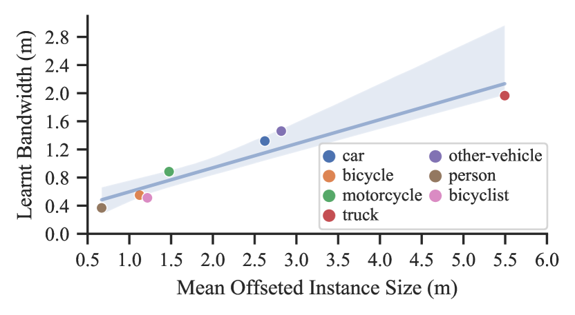
Figure 5: Proportional Relationship Between Sizes and the Learned Bandwidths. The $x$-axis represents the class-wise average size of regressed centers of instances while the $y$-axis stands for the average learned bandwidth of different things classes.

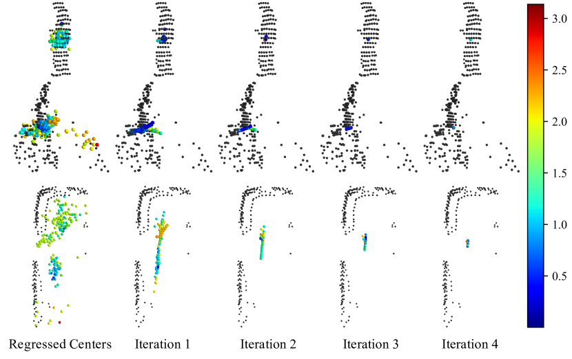
Figure 6: Visualization of Dynamic Shifting Iterations. The black points are the original LiDAR point clouds of instances. The colored points are seeding points. From left to right, with the iteration number increases, the seeding points converge to cluster centers.

Visualization of Dynamic Shifting Iterations. As visualized in Fig. 6, the black points are the original point clouds of different instances including person, bicyclist and car. The seeding points are colored in spectral colors where the redder points represents higher learned bandwidth and bluer points represents lower learned bandwidth. The seeding points farther away from the instance centers tend to learn higher bandwidths in order to quickly converge. While the well-learned regressed points tend to have lower bandwidths to maintain their positions. After four iterations, the seeding points have converged around the instance centers. More visualization results could be found in supplementary materials.

5 Conclusion

With the goal of providing holistic perception for autonomous driving, we are one of the first to address the task of LiDAR-based panoptic segmentation. In order to tackle the challenge brought by the non-uniform distributions of LiDAR point clouds, we propose the novel DS-Net which is specifically designed for effective panoptic segmentation of LiDAR point clouds. Our DS-Net adopts strong baseline design which provides strong support for the consensus-driven fusion module and the novel dynamic shifting module. The novel dynamic shifting module adaptively shifts regressed centers of instances with different density and varying sizes. The consensus-driven fusion efficiently unifies semantic and instance results into panoptic segmentation results. The DS-Net outperforms all strong baselines on both SemanticKITTI and nuScenes. Further analyses show the robustness of the dynamic shifting module and the interpretability of the learned bandwidths.

Appendix

In this appendix, we provide the following sections for a better understanding of the main paper. Firstly, the details of the heuristic clustering algorithms mentioned in the main paper are provided (Sec. 1). Then, we provide analyses of the differentiability of the dynamic shifting to give some insights into our design (Sec. 2). We further analyze the number of iterations in the dynamic shifting module (Sec. 3). Moreover, we report the implementation details of DS-Net for the reproducibility (Sec. 4). Last but not least, the per-class results are reported (Sec. 5), and more visualization examples are displayed (Sec. 6).

1 Details of Heuristic Clustering Algorithms

Breadth First Search (BFS). BFS is simple but effective for indoor point clouds. For the points to be clustered, BFS first constructs a graph where edges connect point pairs that are closer than a given radius. Then each connected sub-graph is considered a cluster. BFS has shown that it is capable of performing high-quality clustering for indoor point clouds [14] which are dense, even and complete. However, it does not apply to LiDAR point clouds. As discussed in the main paper, large density difference within and between clusters means that the fixed radius can not properly adapt to different clusters. Therefore, it is not a good idea to use BFS as the clustering algorithm for autonomous driving scenes.

DBSCAN [11] and HDBSCAN [6]. Both DBSCAN and HDBSCAN are density-based clustering algorithms which make them perform badly on LiDAR point clouds. Similar to BFS, DBSCAN also constructs a graph based on the mutual distances of the points. Although the new concept of core point is introduced to filter out noise points, the problem brought by the fixed radius also occurs in this algorithm. Moreover, the mechanism of noise points recognition also brings problems. For any points to be clustered, if there exists less than a certain number of points within a certain radius, the point is labeled as a noise point. However, the number and densities of points inside instances vary greatly, which makes it hard to determine the line between instances with little points and noise points.

HDBSCAN has a more complex rule of constructing graphs and is claimed to be more robust to density changing than DBSCAN. The mutual reachable distance replaced euclidean distance as the indicators of graph construction, which makes it more robust to density changes. Moreover, with the help of the cluster hierarchy, DBSCAN can automatically adapt to data with different distributions. However, by introducing the concept of mutual reachable distance, HDBSCAN intuitively assumes that the points with lower density are more likely to be seas (noise points) that separate lands (valid clusters), which is not the case in LiDAR point clouds where low-density point clouds can also be valid instances that are far away from the LiDAR sensor. Thus DBSCAN and HDBSCAN can not provide high-quality clustering results.

Mean Shift [8]. Mean Shift performs clustering in a very different way than the above three algorithms. Firstly, seeding points are sampled from the points to be clustered. Then, seeding points are iteratively shifted towards cluster centers in order to obtain centers of all clusters. The positions where seeding points are shifted to is calculated by applying the kernel function on corresponding points. In our implementation, we use the flat kernel which takes the mean of all points within a query ball as the result. The radius of the ball is denoted bandwidth. After several iterations, all the shifted points have converged and the cluster centers are extracted from the converged points. All the points to be clustered are assigned to the nearest cluster centers, which produces the final instance IDs. The advantage of Mean Shift is that the kernel function is not sensitive to density changes and robust to noise points, which makes it more suitable than density-based clustering algorithms.

However, Mean Shift is not perfect. The choice of parameters of the kernel function, which is the bandwidth in this case, is not trivial. The bandwidth controls the range that the kernel function is applied on. Small bandwidth would mislead the regressed centers of a single instance shifting to several different cluster centers and cause over-segmentation. On the contrary, large bandwidth would mislead regressed centers of neighboring instances shifting to one cluster center and result in under-segmentation. The performance of the classes with relatively small size drops with the bandwidth increasing and vice versa. Therefore, the fixed bandwidth can not handle large and small instances simultaneously. Besides, assigning each point to the cluster centers is not reasonable for that nearby instances may have different sizes which would lead to a different degree of dispersion of regressed centers. For example, edge points of a large instance may be farther to its center than that of nearby instances. Although Mean Shift is not as bad as density-based clustering algorithms, there remains a lot of room for improvement.

2 Gradient Calculation of Dynamic Shifting

In this chapter, we are going to show the gradients of one dynamic shifting iteration and that directly regressing bandwidth with flat kernel is not differentiable. The forward pass of dynamic shifting can be broken down to the following steps:

$$K_{j} =(XX^{T}\leq\delta_{j})$$ (6)

$$D_{j} =K_{j}\mathbf{1}$$ (7)

$$S_{j} =D_{j}^{-1}K_{j}X$$ (8)

$$w_{j} =f(F,p_{j})$$ (9)

$$W_{j} =w_{j}\mathbf{1}^{1\times 3}$$ (10)

$$Y_{j} =W_{j}\odot S_{j}$$ (11)

$$Y =\sum_{j=1}^{l}Y_{j}\text{,}$$ (12)

where $X$ represents the seeding points, $f$ is the combination of Softmax and MLP, $p_{j}$ is the parameter of $f$, $F$ is the backbone features, $Y$ is the shifted seeding points, and $\odot$ denotes element-wise product. It is worth noting that $S_{j}$, which is defined by equation 6, 7 and 8, is constant and therefore does not have gradients. Assuming $c$ is the loss, backpropagation gradients are calculated as follows.

$$\frac{\partial c}{\partial F} =\frac{\partial f(F,p_{j})}{\partial F}\frac{\partial c}{\partial w_{j}}$$ (13)

$$\frac{\partial c}{\partial p_{j}} =\frac{\partial f(F,p_{j})}{\partial p_{j}}\frac{\partial c}{\partial w_{j}}$$ (14)

$$\frac{\partial c}{\partial w_{j}} =\frac{\partial c}{\partial W_{j}}\mathbf{1}^{3\times 1}$$ (15)

$$\frac{\partial c}{\partial W_{j}} =S_{j}\odot\frac{\partial c}{\partial Y_{j}}$$ (16)

$$\frac{\partial c}{\partial Y_{j}} =\frac{\partial c}{\partial Y}$$ (17)

However, if the bandwidth $\delta$ is learnable, then equation 6 will turn to:

$$K=(XX^{T}\leq\delta)\text{,}$$ (18)

which unfortunately is not differentiable. Therefore, in our ablation study, in order to further demonstrate that direct regression is not a good strategy, we adopt the Gaussian kernel which is formally defined as:

$$K=exp(-\frac{XX^{T}}{2\delta^{2}})\text{,}$$ (19)

where $\delta$ is the learnable bandwidth. With the Gaussian kernel, the direct regression version of dynamic shifting is now differentiable.

3 Further Analyses of the Number of Iterations

Number of Iterations Settings. In the dynamic shifting module, other than bandwidth candidates, the hyper-parameter to tune is the number of iterations, which is essential for the final clustering quality because too few iterations would cause insufficient convergence while too many iterations would add unnecessary time and space complexity. As shown in Table 5, we experiment on several different iteration number settings. The best result is achieved when the number of iterations is set to 4 which is the counterpoint of sufficient convergence and efficiency.

Table 5: Experiments on the number of iteration. All results in [%].

Number of Iteration	PQ	PQ$\dagger$	RQ	SQ	mIoU
1	57.0	62.6	67.4	77.3	63.5
2	57.6	63.1	67.8	77.5	63.6
3	57.7	63.3	68.0	77.6	63.4
4	57.7	63.4	68.0	77.6	63.5
5	57.5	63.2	67.7	77.6	63.4

Learned Bandwidths of Different Iterations. The average learned bandwidths of different iterations are shown in Fig. 7. As expected, as the iteration rounds grow, points of the same instance gather tighter which usually require smaller bandwidths. After four iterations, learned bandwidths of most classes have dropped to 0.2, which is the lowest they can get, meaning that four iterations are enough for things points to converge to cluster centers, which further validates the conclusion made in the last paragraph.

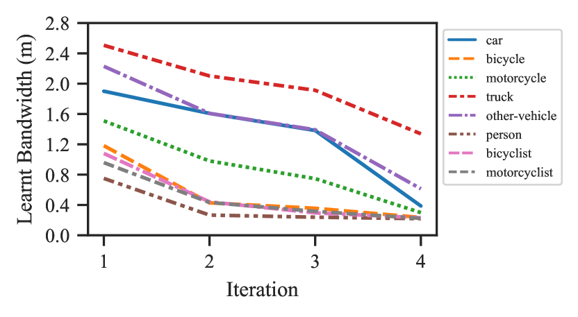
Figure 7: Relationship Between Iterations and the Learned Bandwidths. With number of iteration increases, the learned bandwidth decreases. At the 4th iteration, the learned bandwidths of most classes drop near the lower limit.

4 Implementation Details

Backbone. For both datasets, each input point is represented as a $4$ dimension vector including XYZ coordinates and the intensity. The backbone voxelizes a single frame to $480\times 360\times 32$ voxels under the cylindrical coordinate system. For that we should not use the information of bounding boxes in this segmentation task, the ground truth center of each instance is approximated by the center of its tight box that parallel to axes which makes a better approximation than the mass centers of the incomplete point clouds. The bandwidth of the Mean Shift used in our backbone method is set to $1.2$. Adam solver is utilized to optimize the network. The minimum number of points in a valid instance is set to 50 for SemanticKITTI and 5 for nuScenes.

Dynamic Shifting Module. The number of the FPS downsampled points in the dynamic shifting module is set to $10000$. The final heuristic clustering algorithm used in the dynamic shifting module is Mean Shift with $0.65$ bandwidth for SemanticKITTI and BFS with $1.2$ radius for nuScenes. Bandwidth candidates are set to $0.2$, $1.7$ and $3.2$ for both datasets. The number of Iterations is set to $4$ for both datasets.

Table 6: Detailed per-class PQ results on the test set of SemanticKITTI.

Method	PQ	car	truck	bicycle	motorcycle	other-vehicle	person	bicyclist	motorcyclist	road	sidewalk	parking	other ground	building	vegetation	trunk	terrain	fence	pole	traffic sign
KPConv[25] + PointPillars[18]	44.5	72.5	17.2	9.2	30.8	19.6	29.9	59.4	22.8	84.6	60.1	34.1	8.8	80.7	77.6	53.9	42.2	49.0	46.2	46.8
RangeNet++[20] + PointPillars[18]	37.1	66.9	6.7	3.1	16.2	8.8	14.6	31.8	13.5	90.6	63.2	41.3	6.7	79.2	71.2	34.6	37.4	38.2	32.8	47.4
KPConv[25] + PV-RCNN[24]	50.2	84.5	21.9	9.9	34.2	25.6	51.1	67.9	43.8	84.9	63.6	37.1	8.4	83.7	78.3	57.5	42.3	51.1	51.0	57.4
PolarNet_seg∗	53.3	88.7	31.7	34.6	50.9	39.1	57.5	68.7	45.1	88.1	59.7	40.5	1.0	85.7	77.7	53.2	39.7	44.8	48.6	57.6
Backbone with Fusion	53.1	90.6	15.8	44.2	46.9	28.5	63.1	67.7	47.6	88.2	59.4	29.5	3.0	82.5	79.0	56.6	42.3	48.1	53.2	63.6
DS-Net	55.9	91.2	28.8	45.4	47.2	34.6	63.6	71.1	58.5	89.1	61.2	32.3	4.0	83.2	79.6	58.3	43.4	50.0	55.2	65.3

Table 7: Detailed per-class RQ results on the test set of SemanticKITTI.

Method	RQ	car	truck	bicycle	motorcycle	other-vehicle	person	bicyclist	motorcyclist	road	sidewalk	parking	other ground	building	vegetation	trunk	terrain	fence	pole	traffic sign
KPConv[25] + PV-RCNN[24]	61.4	94.5	26.9	14.5	43.6	32.0	70.0	76.8	52.6	91.5	78.7	47.7	11.4	90.2	94.1	76.4	56.5	66.8	68.8	74.1
PolarNet_seg∗	64.2	96.2	36.0	48.5	58.6	43.0	66.2	77.1	50.3	96.3	74.8	54.2	1.7	92.1	94.1	72.6	53.9	61.1	66.0	76.3
Backbone with Fusion	64.5	97.4	20.5	61.1	57.2	33.2	74.0	75.6	57.8	96.2	75.1	39.2	5.0	88.8	95.5	75.8	57.1	63.8	72.2	80.4
DS-Net	66.7	97.5	32.4	62.2	56.3	38.9	74.3	78.4	62.7	96.8	76.7	42.6	6.4	89.3	95.7	77.5	58.3	65.5	74.0	81.9

Table 8: Detailed per-class SQ results on the test set of SemanticKITTI.

Method	SQ	car	truck	bicycle	motorcycle	other-vehicle	person	bicyclist	motorcyclist	road	sidewalk	parking	other ground	building	vegetation	trunk	terrain	fence	pole	traffic sign
KPConv[25] + PV-RCNN[24]	80.0	89.4	81.3	68.1	78.4	79.8	73.0	88.4	83.3	92.9	80.8	77.8	73.4	92.8	83.2	75.2	75.0	76.5	74.2	77.5
PolarNet_seg∗	81.1	92.2	88.0	71.4	86.9	90.8	87.0	89.1	89.8	91.4	79.9	74.8	55.4	93.1	82.6	73.3	73.8	73.2	73.6	75.5
Backbone with Fusion	80.3	93.0	77.0	72.3	81.9	85.8	85.3	89.5	82.5	91.8	79.1	75.1	60.2	92.9	82.7	74.7	74.0	75.5	73.6	79.1
DS-Net	82.3	93.6	88.9	73.0	83.8	89.0	85.6	90.7	93.3	92.0	79.8	75.8	61.4	93.2	83.2	75.2	74.4	76.3	74.5	79.7

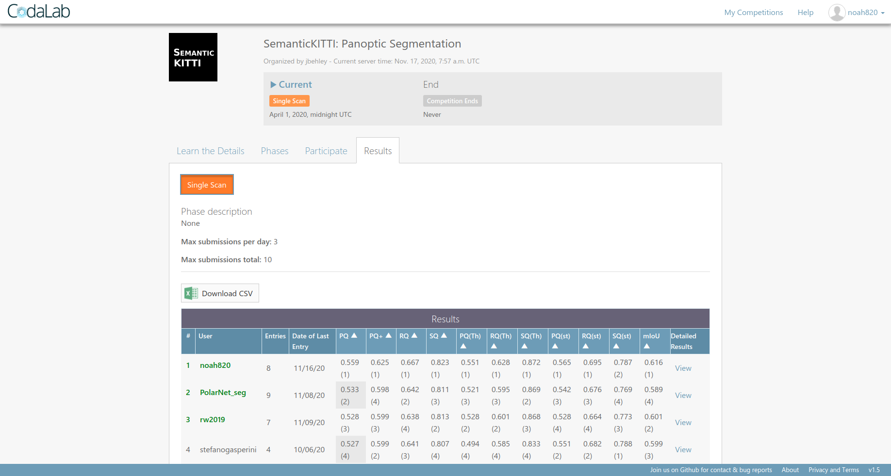
Figure 8: Screenshot of the public leaderboard (https://competitions.codalab.org/competitions/24025) of SemanticKITTI at 2020-11-16. Our method achieves 1st place.

5 Per-class Evaluation Results

Detailed per-class PQ, RQ and SQ results are presented in table 6, 7 and 8 respectively. All the results are reported on the held-out test set of SemanticKITTI. “$\ast$” denotes the unpublished method which is in 2nd place on the public benchmark of SemanticKITTI (accessed on 2020-11-16). Compared to semantic segmentation + detection baseline methods, our DS-Net has huge advantages in things classes in terms of PQ, RQ and SQ. With the help of the dynamic shifting module, our DS-Net surpasses the backbone (with fusion module) in all classes in all three metrics, which demonstrates the effectiveness of the novel dynamic shifting module. Moreover, our DS-Net shows superiority in most classes compared with 2nd place method “Polarnet_seg”. Fig. 8 gives the screenshot of the public leaderboard of SemanticKITTI at 2020-11-16 and our DS-Net achieves 1st place.

6 More Visualization Results of the DS-Net

We further show the qualitative comparison of our backbone and DS-Net. As shown in Fig. 9, 10 and 11, a total of 9 LiDAR frames from the validation set of SemanticKITTI are taken out for visualization. The left columns are the visualization of the results of our bare backbone with the consensus-driven fusion module. The middle columns show the results of the DS-Net and the right columns are the ground truth. For each frame, a region of interest (as framed in red) is zoomed in to show that our DS-Net is capable of correctly handling instances with different sizes and densities while our backbone method tends to either oversegment or undersegment in these complex cases. Please note that all the stuff classes points are colored following the official definition while the colors of things instances are randomly picked. To highlight the segmentation results of things classes in the regions of interest, we only color the things class points while the stuff class points are colored as gray. Since the order of the predicted instance IDs is different from that of the ground truth, the colors of the things instances cannot correspond in predictions and the ground truth.

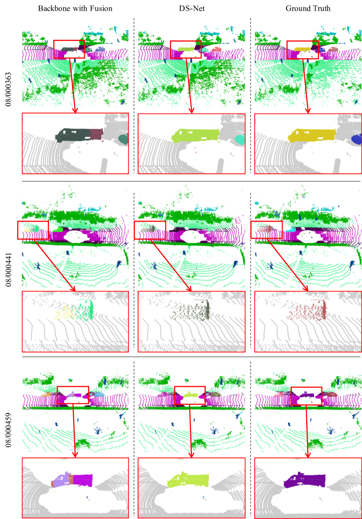
Figure 9: Qualitative Comparison of the Backbone and DS-Net (1).

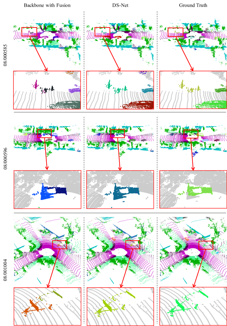
Figure 10: Qualitative Comparison of the Backbone and DS-Net (2).

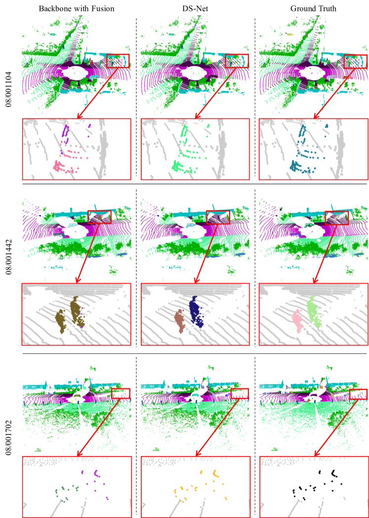
Figure 11: Qualitative Comparison of the Backbone and DS-Net (3).

References

- [1] Iro Armeni, Ozan Sener, Amir R Zamir, Helen Jiang, Ioannis Brilakis, Martin Fischer, and Silvio Savarese. 3d semantic parsing of large-scale indoor spaces. In Proceedings of the IEEE Conference on Computer Vision and Pattern Recognition, pages 1534–1543, 2016.
- [2] Jens Behley, Martin Garbade, Andres Milioto, Jan Quenzel, Sven Behnke, Cyrill Stachniss, and Jurgen Gall. Semantickitti: A dataset for semantic scene understanding of lidar sequences. In Proceedings of the IEEE International Conference on Computer Vision, pages 9297–9307, 2019.
- [3] Jens Behley, Andres Milioto, and Cyrill Stachniss. A benchmark for lidar-based panoptic segmentation based on kitti. arXiv preprint arXiv:2003.02371, 2020.
- [4] Maxim Berman, Amal Rannen Triki, and Matthew B Blaschko. The lovász-softmax loss: A tractable surrogate for the optimization of the intersection-over-union measure in neural networks. In Proceedings of the IEEE Conference on Computer Vision and Pattern Recognition, pages 4413–4421, 2018.
- [5] Holger Caesar, Varun Bankiti, Alex H. Lang, Sourabh Vora, Venice Erin Liong, Qiang Xu, Anush Krishnan, Yu Pan, Giancarlo Baldan, and Oscar Beijbom. nuscenes: A multimodal dataset for autonomous driving. arXiv preprint arXiv:1903.11027, 2019.
- [6] Ricardo JGB Campello, Davoud Moulavi, and Jörg Sander. Density-based clustering based on hierarchical density estimates. In Pacific-Asia conference on knowledge discovery and data mining, pages 160–172. Springer, 2013.
- [7] Christopher Choy, JunYoung Gwak, and Silvio Savarese. 4d spatio-temporal convnets: Minkowski convolutional neural networks. In Proceedings of the IEEE Conference on Computer Vision and Pattern Recognition, pages 3075–3084, 2019.
- [8] Dorin Comaniciu and Peter Meer. Mean shift: A robust approach toward feature space analysis. IEEE Transactions on pattern analysis and machine intelligence, 24(5):603–619, 2002.
- [9] Angela Dai, Angel X Chang, Manolis Savva, Maciej Halber, Thomas Funkhouser, and Matthias Nießner. Scannet: Richly-annotated 3d reconstructions of indoor scenes. In Proceedings of the IEEE Conference on Computer Vision and Pattern Recognition, pages 5828–5839, 2017.
- [10] Francis Engelmann, Martin Bokeloh, Alireza Fathi, Bastian Leibe, and Matthias Nießner. 3d-mpa: Multi-proposal aggregation for 3d semantic instance segmentation. In Proceedings of the IEEE/CVF Conference on Computer Vision and Pattern Recognition, pages 9031–9040, 2020.
- [11] Martin Ester, Hans-Peter Kriegel, Jörg Sander, Xiaowei Xu, et al. A density-based algorithm for discovering clusters in large spatial databases with noise. In Kdd, volume 96, pages 226–231, 1996.
- [12] Lei Han, Tian Zheng, Lan Xu, and Lu Fang. Occuseg: Occupancy-aware 3d instance segmentation. In Proceedings of the IEEE/CVF Conference on Computer Vision and Pattern Recognition, pages 2940–2949, 2020.
- [13] Qingyong Hu, Bo Yang, Linhai Xie, Stefano Rosa, Yulan Guo, Zhihua Wang, Niki Trigoni, and Andrew Markham. Randla-net: Efficient semantic segmentation of large-scale point clouds. In Proceedings of the IEEE/CVF Conference on Computer Vision and Pattern Recognition, pages 11108–11117, 2020.
- [14] Li Jiang, Hengshuang Zhao, Shaoshuai Shi, Shu Liu, Chi-Wing Fu, and Jiaya Jia. Pointgroup: Dual-set point grouping for 3d instance segmentation. In Proceedings of the IEEE/CVF Conference on Computer Vision and Pattern Recognition, pages 4867–4876, 2020.
- [15] Alexander Kirillov, Kaiming He, Ross Girshick, Carsten Rother, and Piotr Dollár. Panoptic segmentation. In Proceedings of the IEEE conference on computer vision and pattern recognition, pages 9404–9413, 2019.
- [16] Shu Kong and Charless C Fowlkes. Recurrent pixel embedding for instance grouping. In Proceedings of the IEEE Conference on Computer Vision and Pattern Recognition, pages 9018–9028, 2018.
- [17] Jean Lahoud, Bernard Ghanem, Marc Pollefeys, and Martin R Oswald. 3d instance segmentation via multi-task metric learning. In Proceedings of the IEEE International Conference on Computer Vision, pages 9256–9266, 2019.
- [18] Alex H Lang, Sourabh Vora, Holger Caesar, Lubing Zhou, Jiong Yang, and Oscar Beijbom. Pointpillars: Fast encoders for object detection from point clouds. In Proceedings of the IEEE Conference on Computer Vision and Pattern Recognition, pages 12697–12705, 2019.
- [19] A. Milioto, J. Behley, C. McCool, and C. Stachniss. Lidar panoptic segmentation for autonomous driving. In IROS, 2020.
- [20] Andres Milioto, Ignacio Vizzo, Jens Behley, and Cyrill Stachniss. Rangenet++: Fast and accurate lidar semantic segmentation. In 2019 IEEE/RSJ International Conference on Intelligent Robots and Systems (IROS), pages 4213–4220. IEEE, 2019.
- [21] Quang-Hieu Pham, Thanh Nguyen, Binh-Son Hua, Gemma Roig, and Sai-Kit Yeung. Jsis3d: joint semantic-instance segmentation of 3d point clouds with multi-task pointwise networks and multi-value conditional random fields. In Proceedings of the IEEE Conference on Computer Vision and Pattern Recognition, pages 8827–8836, 2019.
- [22] Charles R Qi, Hao Su, Kaichun Mo, and Leonidas J Guibas. Pointnet: Deep learning on point sets for 3d classification and segmentation. In Proceedings of the IEEE conference on computer vision and pattern recognition, pages 652–660, 2017.
- [23] Charles Ruizhongtai Qi, Li Yi, Hao Su, and Leonidas J Guibas. Pointnet++: Deep hierarchical feature learning on point sets in a metric space. In Advances in neural information processing systems, pages 5099–5108, 2017.
- [24] Shaoshuai Shi, Chaoxu Guo, Li Jiang, Zhe Wang, Jianping Shi, Xiaogang Wang, and Hongsheng Li. Pv-rcnn: Point-voxel feature set abstraction for 3d object detection. In Proceedings of the IEEE/CVF Conference on Computer Vision and Pattern Recognition, pages 10529–10538, 2020.
- [25] Hugues Thomas, Charles R Qi, Jean-Emmanuel Deschaud, Beatriz Marcotegui, François Goulette, and Leonidas J Guibas. Kpconv: Flexible and deformable convolution for point clouds. In Proceedings of the IEEE International Conference on Computer Vision, pages 6411–6420, 2019.
- [26] Weiyue Wang, Ronald Yu, Qiangui Huang, and Ulrich Neumann. Sgpn: Similarity group proposal network for 3d point cloud instance segmentation. In Proceedings of the IEEE Conference on Computer Vision and Pattern Recognition, pages 2569–2578, 2018.
- [27] Xinlong Wang, Shu Liu, Xiaoyong Shen, Chunhua Shen, and Jiaya Jia. Associatively segmenting instances and semantics in point clouds. In Proceedings of the IEEE Conference on Computer Vision and Pattern Recognition, pages 4096–4105, 2019.
- [28] Yue Wang, Yongbin Sun, Ziwei Liu, Sanjay E Sarma, Michael M Bronstein, and Justin M Solomon. Dynamic graph cnn for learning on point clouds. Acm Transactions On Graphics (tog), 38(5):1–12, 2019.
- [29] Kelvin Wong, Shenlong Wang, Mengye Ren, Ming Liang, and Raquel Urtasun. Identifying unknown instances for autonomous driving. In The Conference on Robot Learning (CORL), 2019.
- [30] Bichen Wu, Alvin Wan, Xiangyu Yue, and Kurt Keutzer. Squeezeseg: Convolutional neural nets with recurrent crf for real-time road-object segmentation from 3d lidar point cloud. In 2018 IEEE International Conference on Robotics and Automation (ICRA), pages 1887–1893. IEEE, 2018.
- [31] Wenxuan Wu, Zhongang Qi, and Li Fuxin. Pointconv: Deep convolutional networks on 3d point clouds. In Proceedings of the IEEE Conference on Computer Vision and Pattern Recognition, pages 9621–9630, 2019.
- [32] Yan Yan, Yuxing Mao, and Bo Li. Second: Sparsely embedded convolutional detection. Sensors, 18(10):3337, 2018.
- [33] Dongsu Zhang, Junha Chun, Sang Kyun Cha, and Young Min Kim. Spatial semantic embedding network: Fast 3d instance segmentation with deep metric learning. arXiv preprint arXiv:2007.03169, 2020.
- [34] Feihu Zhang, Chenye Guan, Jin Fang, Song Bai, Ruigang Yang, Philip Torr, and Victor Prisacariu. Instance segmentation of lidar point clouds. ICRA, Cited by, 4(1), 2020.
- [35] Yang Zhang, Zixiang Zhou, Philip David, Xiangyu Yue, Zerong Xi, Boqing Gong, and Hassan Foroosh. Polarnet: An improved grid representation for online lidar point clouds semantic segmentation. In Proceedings of the IEEE/CVF Conference on Computer Vision and Pattern Recognition, pages 9601–9610, 2020.
- [36] Lin Zhao and Wenbing Tao. Jsnet: Joint instance and semantic segmentation of 3d point clouds. In AAAI, pages 12951–12958, 2020.
- [37] Hui Zhou, Xinge Zhu, Xiao Song, Yuexin Ma, Zhe Wang, Hongsheng Li, and Dahua Lin. Cylinder3d: An effective 3d framework for driving-scene lidar semantic segmentation. arXiv preprint arXiv:2008.01550, 2020.