Peculiarity of Symmetric Ring Systems with Double Y-Junctions and the magnetic effects

Abstract

We discuss quantum dynamics in the ring systems with double Y-junctions in which two arms have same length. The node of a Y-junction can be parametrized by U(3). Considering mathematically permitted junction conditions seriously, we formulate such systems by scattering matrices. We show that the symmetric ring systems, which consist of two nodes with the same parameters under the reflection symmetry, have remarkable aspects that there exist localized states inevitably, and resonant perfect transmission occurs when the wavenumber of an incoming wave coincides with that of the localized states, for any parameters of the nodes except for the extremal cases in which the absolute values of components of scattering matrices take $1$. We also investigate the magnetic disturbance to the symmetric ring systems.

1 Introduction

Quantum mechanical features in non-simply connected, ring geometries have attracted great interest from many physicists. Particularly striking phenomena in ring systems are induced by the Aharonov-Bohm effect [1] and the Aharonov-Casher effect [2]. To prove these effects, ring systems have been realized in semiconductor nanotechnology (see e.g., [3, 4]). More recently, various physical characteristics of quantum ring systems have also been investigated in [5, 6, 7]. Furthermore, applications of ring systems to a qubit were discussed [8, 9]. A typical structure of ring systems is formed by connected double Y-junctions. A Y-junction is composed of three one-dimensional quantum wires intersecting at one point (i.e. a node). We shed light on such quantum ring systems with double Y-junctions.

Quantum ring systems with Y-junctions were originally investigated in the pioneer theoretical works [10, 11]. At a node, a simple form of the scattering matrices had been customary assumed for years in the literature. On the other hand, mathematical features of point interactions at a node were thoroughly investigated in [12, 13, 14, 15]. These works showed that the point interaction on a Y-junction can be parametrized by U(3). In subsequent works, certain aspects of transmission properties of a quantum particle in the system of a single Y-junction were studied in [16], and a star graph and related topics were also discussed in [17, 18, 19, 20]. Ring systems with double Y-junctions were restudied in [21] based on the mathematical framework. However, the previous work [21] is restricted to a subclass in parameter space of U(3), i.e., the scale invariant class. Therefore, in this paper, we provide a more general discussion of quantum ring systems with double Y-junctions without the tight restriction on the parameter space.

We formulate quantum dynamics in the ring systems with double Y-junctions, taking account of mathematically permitted junction conditions seriously. While we assume that the two arms of a ring has the same length, we do not impose any restriction on the parameters of two nodes from the beginning. From our analysis, we find that the symmetric ring systems, which have two same nodes under the reflection symmetry, have remarkable features that localized states exist inevitably and that resonant perfect transmission occurs for any parameters of the nodes except for the extremal cases in which the absolute values of components of scattering matrices take $1$. We also discuss disturbance to the symmetric ring systems. In particular, we investigate the effect of magnetic flux which penetrates the ring systems. From our analysis, we find the general expressions of the amplitudes for reflection and transmission in the presence of the magnetic flux. This paper is organized as follows. In Sec. 2, we review the formulation by scattering matrices based on [21]. In Sec. 3, we investigate localized states and show that the existence of the localized states is inevitable in the symmetric ring systems. In Sec. 4, focusing on scattering problems in the symmetric ring systems, we investigate the transmission probability through the ring systems. Then we find that the resonant perfect transmission occurs when the wavenumber of an incoming wave coincides with that of localized states. In Sec. 5, we consider external magnetic fields as disturbance to the ring systems. Formulating the quantum ring systems in the presence of the magnetic fields, we investigate probability amplitudes for reflection and transmission. Finally, we give a conclusion in Sec. 6.

2 Formulation of a quantum particle in a ring system with double Y-junctions

2.1 The coordinate system and the basic equation

We discuss a ring system with double Y-junctions as shown in Fig. 1. Three one-dimensional quantum wires intersect at one point (i.e., node) in each Y-junction. We describe the Y-junction on the left-hand side by the inward coordinate axes $x_{1},x_{2}$ and $x_{3}$, and that on the right-hand side by the outward coordinate axes $x_{2},x_{3}$ and $x_{4}$, as shown in Fig. 2(a) and (b), respectively. Note that the angle between any two axes and the curvature of the wires have no effect on the physical states. We assume that the nodes locate at $x_{i}=\xi_{\rm\rm I}$ ($i=1,2,3$) and at $x_{j}=\xi_{\rm\rm I\!I}$ ($j=2,3,4$), where $\xi_{\rm\rm I}>\xi_{\rm\rm I\!I}$. We consider a free quantum particle on this system, which obeys the Schrödinger equation on the wires,

$$i\hbar\frac{\partial}{\partial t}\Phi_{i}(t,x_{i})=-\frac{\hbar^{2}}{2m}\frac{\partial^{2}}{\partial x_{i}^{2}}\Phi_{i}(t,x_{i})\quad(i=1,2,3,4),$$ (1)

where $\Phi_{i}$ denotes the wave function on the $x_{i}$-axis, and $m$ denotes the mass of the particle.

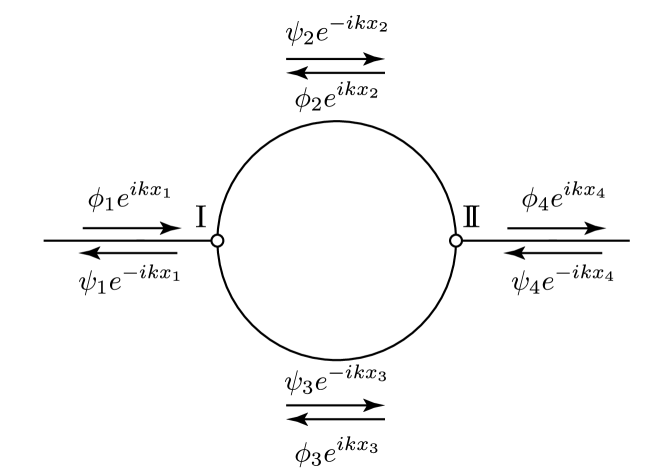
Figure 1: A ring system with double Y-junctions. This ring has two nodes (I and II). Plane waves on this system are expressed by $\phi_{1}e^{ikx_{1}}$, $\psi_{1}e^{-ikx_{1}}$, $\phi_{2}e^{ikx_{2}}$, $\psi_{2}e^{-ikx_{2}}$, $\phi_{3}e^{ikx_{3}}$, $\psi_{3}e^{-ikx_{3}}$, $\phi_{4}e^{ikx_{4}}$, and $\psi_{4}e^{-ikx_{4}}$.

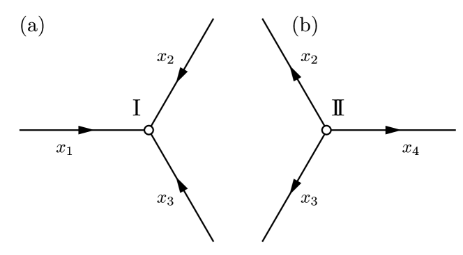
Figure 2: (a) The coordinate axes for the node I. (b) The coordinate axes for the node II.

2.2 Junction conditions

At the nodes, we have to impose the junction conditions, which are provided by the conservation of probability current, i.e.,

$$\displaystyle\sum_{i=1}^{3}\lim_{x_{i}\rightarrow\xi_{\rm I}^{-}}j_{i}(t,x_{i})=0,$$ (2)

$$\displaystyle\sum_{i=2}^{4}\lim_{x_{i}\rightarrow\xi_{\rm I\!I}^{+}}j_{i}(t,x_{i})=0,$$ (3)

where $x_{i}\rightarrow\xi_{\rm I}^{-}$ denotes the limit from below, and $x_{i}\rightarrow\xi_{\rm I\!I}^{+}$ denotes the limit from above. The probability current $j_{i}$ is defined by

$$j_{i}(t,x_{i}):=-\frac{i\hbar}{2m}\left\{\Phi^{\ast}_{i}(t,x_{i})\partial_{x}\Phi_{i}(t,x_{i})-\left(\partial_{x}\Phi^{\ast}_{i}(t,x_{i})\right)\Phi_{i}(t,x_{i})\right\}.$$ (4)

The junction conditions (2) and (3) can be expressed by [15]

$$\Psi^{\prime\dagger}\Psi-\Psi^{\dagger}\Psi^{\prime}=0,$$ (5)

where for the Y-junction $(x_{1}x_{2}x_{3})$ (node I), we should take

$$\Psi:=\lim_{x\rightarrow\xi_{\rm I}^{-}}\left(\begin{array}[]{c}\Phi_{2}(t,x)\\ \Phi_{3}(t,x)\\ \Phi_{1}(t,x)\end{array}\right),\ \Psi^{\prime}:=\lim_{x\rightarrow\xi_{\rm I}^{-}}\left(\begin{array}[]{c}\partial_{x}\Phi_{2}(t,x)\\ \partial_{x}\Phi_{3}(t,x)\\ \partial_{x}\Phi_{1}(t,x)\end{array}\right),$$ (6)

and for the Y-junction $(x_{4}x_{2}x_{3})$ (node $\rm I\!I$), we should take

$$\Psi:=\lim_{x\rightarrow\xi_{\rm I\!I}^{+}}\left(\begin{array}[]{c}\Phi_{2}(t,x)\\ \Phi_{3}(t,x)\\ \Phi_{4}(t,x)\end{array}\right),\ \Psi^{\prime}:=\lim_{x\rightarrow\xi_{\rm I\!I}^{+}}\left(\begin{array}[]{c}\partial_{x}\Phi_{2}(t,x)\\ \partial_{x}\Phi_{3}(t,x)\\ \partial_{x}\Phi_{4}(t,x)\end{array}\right).$$ (7)

Note that the above ordering of the axes in $\Psi$ and $\Psi^{\prime}$ is different from that in the previous work [21]. The present ordering is useful to deal with external magnetic effects as seen below. Equation (5) is equivalently expressed as [15]

$$\left|\Psi-iL_{0}\Psi^{\prime}\right|=\left|\Psi+iL_{0}\Psi^{\prime}\right|,$$ (8)

where $L_{0}(\in\mathbb{R})$ is a nonzero, arbitrary constant with dimension of length, which can be regarded as a gauge freedom [21] and, therefore, does not appear in physical quantities [15]. Equation (8) means that $\Psi-iL_{0}\Psi^{\prime}$ is connected to $\Psi+iL_{0}\Psi^{\prime}$ via a unitary transformation. Thus, we obtain the junction condition [15]

$$(U-I_{3})\Psi+iL_{0}(U+I_{3})\Psi^{\prime}=0,$$ (9)

where $I_{3}$ is the $3\times 3$ identity matrix, and $U$ is a $3\times 3$ unitary matrix. Therefore, the junction condition (9) is characterized by the unitary matrix $U\in{\rm U}(3)$.

Let us also discuss a parametrization of the unitary matrix $U$. Based on the discussion in [21], we adopt the following parametrization. On the Y-junction $(x_{1}x_{2}x_{3})$ (node I), we take

$$U=VDV^{\dagger},$$ (10)

where

$$D:={\rm diag}\left(e^{i\theta_{(1)}},e^{i\theta_{(2)}},e^{i\theta_{(3)}}\right),$$ (11)

and

$$V:=e^{i\alpha\lambda_{3}}e^{i\beta\lambda_{2}}e^{i\gamma\lambda_{3}}e^{i\delta\lambda_{5}}e^{ia\lambda_{3}}e^{ib\lambda_{2}}.$$ (12)

Here, $\theta_{(1)}$, $\theta_{(2)}$, $\theta_{(3)}$, $\alpha$, $\beta$, $\gamma$, $\delta$, $a$, $b$ $\in\mathbb{R}$, and $\lambda_{2},\lambda_{3}$, and $\lambda_{5}$ are the Gell-Mann Matrices (see [21] in detail). In the same way, on the Y-junction $(x_{4}x_{2}x_{3})$ (node II), we take

$$U=\tilde{V}\tilde{D}\tilde{V}^{\dagger},$$ (13)

where

$$\tilde{D}:={\rm diag}\left(e^{i\tilde{\theta}_{(1)}},e^{i\tilde{\theta}_{(2)}},e^{i\tilde{\theta}_{(3)}}\right),$$ (14)

and

$$\tilde{V}:=e^{i\tilde{\alpha}\lambda_{3}}e^{i\tilde{\beta}\lambda_{2}}e^{i\tilde{\gamma}\lambda_{3}}e^{i\tilde{\delta}\lambda_{5}}e^{i\tilde{a}\lambda_{3}}e^{i\tilde{b}\lambda_{2}}.$$ (15)

Here $\tilde{\theta}_{(1)}$, $\tilde{\theta}_{(2)}$, $\tilde{\theta}_{(3)}$, $\tilde{\alpha}$, $\tilde{\beta}$, $\tilde{\gamma}$, $\tilde{\delta}$, $\tilde{a}$, $\tilde{b}$ $\in\mathbb{R}$. Therefore, the junction condition (9) with the unitary matrix $U$ is characterized by the nine real parameters ($\theta_{(1)}$, $\theta_{(2)}$, $\theta_{(3)}$, $\alpha$, $\beta$, $\gamma$, $\delta$, $a$, $b$), or ($\tilde{\theta}_{(1)}$, $\tilde{\theta}_{(2)}$, $\tilde{\theta}_{(3)}$, $\tilde{\alpha}$, $\tilde{\beta}$, $\tilde{\gamma}$, $\tilde{\delta}$, $\tilde{a}$, $\tilde{b}$).

2.3 Scattering matrices

2.3.1 The scattering matrix for a single Y-junction

We consider a quantum state on the coordinate system for the node I (see Fig. 2(a)). We assume that incoming waves and outgoing waves are provided by $\phi_{i}e^{ikx_{i}}$ and $\psi_{i}e^{-ikx_{i}}$ ($\phi_{i},\psi_{i}\in\mathbb{C}$ and $i=1,2,3$ ), respectively. Then we have

$$\Phi_{i}(t,x_{i})=e^{-i\frac{\cal E}{\hbar}t}\left(\phi_{i}e^{ikx_{i}}+\psi_{i}e^{-ikx_{i}}\right),$$ (16)

where ${\cal E}:=\hbar^{2}k^{2}/2m$. From this expression, we derive

$$\Psi=e^{-i\frac{\cal E}{\hbar}t}\left\{e^{ik\xi_{\rm I}}\left(\begin{array}[]{c}\phi_{2}\\ \phi_{3}\\ \phi_{1}\end{array}\right)+e^{-ik\xi_{\rm I}}\left(\begin{array}[]{c}\psi_{2}\\ \psi_{3}\\ \psi_{1}\end{array}\right)\right\},$$ (17)

$$\Psi^{\prime}=e^{-i\frac{\cal E}{\hbar}t}\left\{ike^{ik\xi_{\rm I}}\left(\begin{array}[]{c}\phi_{2}\\ \phi_{3}\\ \phi_{1}\end{array}\right)-ike^{-ik\xi_{\rm I}}\left(\begin{array}[]{c}\psi_{2}\\ \psi_{3}\\ \psi_{1}\end{array}\right)\right\}.$$ (18)

By substituting Eqs. (17) and (18) into Eq. (9), we can define the $S$-matrix $S_{\rm I}$ by the equation

$$\left(\begin{array}[]{c}\psi_{2}\\ \psi_{3}\\ \psi_{1}\end{array}\right)=S_{\rm I}\left(\begin{array}[]{c}\phi_{2}\\ \phi_{3}\\ \phi_{1}\end{array}\right).$$ (19)

Using Eqs. (10), (11), and (12), we derive

$$S_{\rm I}=e^{2ik\xi_{\rm I}}VS_{\rm(0)I}V^{\dagger},$$ (20)

where

$$S_{\rm(0)I}:={\rm diag}\left(\frac{ikL_{(1)}+1}{ikL_{(1)}-1},\frac{ikL_{(2)}+1}{ikL_{(2)}-1},\frac{ikL_{(3)}+1}{ikL_{(3)}-1}\right).$$ (21)

Here we define

$$L_{(i)}:=L_{0}\cot\frac{\theta_{(i)}}{2}.$$ (22)

When we write $S_{\rm I}$ in the form

$$S_{\rm I}=\left(\begin{array}[]{ccc}s_{22}&s_{23}&s_{21}\\ s_{32}&s_{33}&s_{31}\\ s_{12}&s_{13}&s_{11}\\ \end{array}\right),$$ (23)

then $s_{ii}$ represents the probability amplitude for reflection from the $x_{i}$-axis to the $x_{i}$-axis, while the $s_{ij}$ ($i\neq j$) represents the probability amplitude for transmission from the $x_{j}$-axis to the $x_{i}$-axis.

Next, we consider a quantum state on the coordinate system for the node II (see Fig. 2(b)). We assume that incoming waves and outgoing waves are provided by $\psi_{i}e^{-ikx_{i}}$ and $\phi_{i}e^{ikx_{i}}$ ($\psi_{i},\phi_{i}\in\mathbb{C}$ and $i=2,3,4$ ), respectively. Then we have

$$\Phi_{i}(t,x_{i})=e^{-i\frac{\cal E}{\hbar}t}\left(\psi_{i}e^{-ikx_{i}}+\phi_{i}e^{ikx_{i}}\right).$$ (24)

From this expression, we derive

$$\Psi=e^{-i\frac{\cal E}{\hbar}t}\left\{e^{-ik\xi_{\rm I\!I}}\left(\begin{array}[]{c}\psi_{2}\\ \psi_{3}\\ \psi_{4}\end{array}\right)+e^{ik\xi_{\rm I\!I}}\left(\begin{array}[]{c}\phi_{2}\\ \phi_{3}\\ \phi_{4}\end{array}\right)\right\},$$ (25)

$$\Psi^{\prime}=e^{-i\frac{\cal E}{\hbar}t}\left\{-ike^{-ik\xi_{\rm I\!I}}\left(\begin{array}[]{c}\psi_{2}\\ \psi_{3}\\ \psi_{4}\end{array}\right)+ike^{ik\xi_{\rm I\!I}}\left(\begin{array}[]{c}\phi_{2}\\ \phi_{3}\\ \phi_{4}\end{array}\right)\right\}.$$ (26)

By substituting Eqs. (25) and (26) into Eq. (9), we can define the $S$-matrix $S_{\rm I\!I}$ by the equation

$$\left(\begin{array}[]{c}\phi_{2}\\ \phi_{3}\\ \phi_{4}\end{array}\right)=S_{\rm I\!I}\left(\begin{array}[]{c}\psi_{2}\\ \psi_{3}\\ \psi_{4}\end{array}\right).$$ (27)

Using Eqs. (13), (14), and (15), we derive

$$S_{\rm I\!I}=e^{-2ik\xi_{\rm I\!I}}\tilde{V}S_{\rm(0)I\!I}\tilde{V}^{\dagger},$$ (28)

where

$$S_{\rm(0)I\!I}:={\rm diag}\left(\frac{ik\tilde{L}_{(1)}-1}{ik\tilde{L}_{(1)}+1},\frac{ik\tilde{L}_{(2)}-1}{ik\tilde{L}_{(2)}+1},\frac{ik\tilde{L}_{(3)}-1}{ik\tilde{L}_{(3)}+1}\right).$$ (29)

Here

$$\tilde{L}_{(i)}:=\tilde{L}_{0}\cot\frac{\tilde{\theta}_{(i)}}{2},$$ (30)

where $\tilde{L}_{0}$ denotes the parameter at the node ${\rm I\!I}$. We can write $S_{\rm I\!I}$ in the form

$$S_{\rm I\!I}=\left(\begin{array}[]{ccc}\tilde{s}_{22}&\tilde{s}_{23}&\tilde{s}_{24}\\ \tilde{s}_{32}&\tilde{s}_{33}&\tilde{s}_{34}\\ \tilde{s}_{42}&\tilde{s}_{43}&\tilde{s}_{44}\\ \end{array}\right),$$ (31)

in common with the node I.

We also show important relations which $S_{\rm I}$ and $S_{\rm I\!I}$ satisfy. Since $S_{\rm I}$ and $S_{\rm I\!I}$ are both unitary, we have

$$S_{\rm I}S_{\rm I}^{\dagger}=S_{\rm I}^{\dagger}S_{\rm I}=I_{3},$$ (32)

$$S_{\rm I\!I}S_{\rm I\!I}^{\dagger}=S_{\rm I\!I}^{\dagger}S_{\rm I\!I}=I_{3}.$$ (33)

These are also expressed as

$$\sum_{k=1}^{3}s_{ik}s_{jk}^{\ast}=\sum_{k=1}^{3}s_{ki}^{\ast}s_{kj}=\delta_{ij},$$ (34)

$$\sum_{k=2}^{4}\tilde{s}_{ik}\tilde{s}_{jk}^{\ast}=\sum_{k=2}^{4}\tilde{s}_{ki}^{\ast}\tilde{s}_{kj}=\delta_{ij}.$$ (35)

These relations are important to derive simplified forms for probability amplitudes in the next section.

2.3.2 The scattering matrix for the ring

In this section, we consider the ring system shown in Fig. 1 as in Fig. 3. The $S$-matrix $S_{\rm R}$ for the ring system is defined by

$$\left(\begin{array}[]{c}\psi_{1}\\ \phi_{4}\end{array}\right)=S_{\rm R}\left(\begin{array}[]{c}\phi_{1}\\ \psi_{4}\end{array}\right),$$ (36)

where $S_{\rm R}$ is a $2\times 2$ matrix. We derive $S_{\rm R}$ in terms of the components of $S_{\rm I}$ and $S_{\rm I\!I}$, i.e., $s_{ij}$ and $\tilde{s}_{ij}$. For this purpose, we define $2\times 2$ matrices $s$ and $\tilde{s}$ as

$$s:=\left(\begin{array}[]{cc}s_{22}&s_{23}\\ s_{32}&s_{33}\end{array}\right),\quad\tilde{s}:=\left(\begin{array}[]{cc}\tilde{s}_{22}&\tilde{s}_{23}\\ \tilde{s}_{32}&\tilde{s}_{33}\end{array}\right).$$ (37)

By decomposing Eqs. (19) and (27) into the components on $x_{1}$ and $x_{4}$ axes and those on $x_{2}$ and $x_{3}$ axes, we can obtain the components of $S_{\rm R}$ as

$$\left(S_{\rm R}\right)_{11} = s_{11}+\left(s_{12}\ \ s_{13}\right)\left(I_{2}-\tilde{s}s\right)^{-1}\tilde{s}\left(\begin{array}[]{c}s_{21}\\ s_{31}\end{array}\right),$$ (40)

$$\left(S_{\rm R}\right)_{12} = \left(s_{12}\ \ s_{13}\right)\left(I_{2}-\tilde{s}s\right)^{-1}\left(\begin{array}[]{c}\tilde{s}_{24}\\ \tilde{s}_{34}\end{array}\right),$$ (43)

$$\left(S_{\rm R}\right)_{21} = \left(\tilde{s}_{42}\ \ \tilde{s}_{43}\right)\left(I_{2}-s\tilde{s}\right)^{-1}\left(\begin{array}[]{c}s_{21}\\ s_{31}\end{array}\right),$$ (46)

$$\left(S_{\rm R}\right)_{22} = \tilde{s}_{44}+\left(\tilde{s}_{42}\ \ \tilde{s}_{43}\right)\left(I_{2}-s\tilde{s}\right)^{-1}s\left(\begin{array}[]{c}\tilde{s}_{24}\\ \tilde{s}_{34}\end{array}\right),$$ (49)

where $I_{2}$ is the $2\times 2$ identity matrix. Here, we assume $|s_{ij}|<1$ and $|\tilde{s}_{ij}|<1$. In this case, $(I_{2}-s\tilde{s})^{-1}$ and $(I_{2}-\tilde{s}s)^{-1}$ are given by

$$(I_{2}-s\tilde{s})^{-1} = \sum_{k=0}^{\infty}\left(s\tilde{s}\right)^{k},$$ (50)

$$(I_{2}-\tilde{s}s)^{-1} = \sum_{k=0}^{\infty}\left(\tilde{s}s\right)^{k}.$$ (51)

While the diagonal components of $S_{\rm R}$ represent the probability amplitude for reflection, the non-diagonal components of $S_{\rm R}$ represent that for transmission.

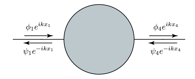
Figure 3: Scattering by a ring system. The gray circle includes the ring.

3 Localized states on the ring

We discuss localized states which could arise on the ring. In these states, while $\Phi_{1}$ and $\Phi_{4}$ vanish (i.e., $\Phi_{1}=\Phi_{4}=0$), the non-zero components $\Phi_{2}$ and $\Phi_{3}$ are given by Eq. (16). The junction conditions at node I and node II are then written as

$$M\left(\begin{array}[]{c}\phi_{2}\\ \psi_{2}\\ \phi_{3}\\ \psi_{3}\end{array}\right)=0,$$ (52)

where

$$M:=\left(\begin{array}[]{cccc}V_{21}^{\ast}\kappa_{1}e^{2ik\xi_{\rm I}}&V_{21}^{\ast}\kappa_{1}^{\ast}&V_{31}^{\ast}\kappa_{1}e^{2ik\xi_{\rm I}}&V_{31}^{\ast}\kappa_{1}^{\ast}\\ V_{22}^{\ast}\kappa_{2}e^{2ik\xi_{\rm I}}&V_{22}^{\ast}\kappa_{2}^{\ast}&V_{32}^{\ast}\kappa_{2}e^{2ik\xi_{\rm I}}&V_{32}^{\ast}\kappa_{2}^{\ast}\\ V_{23}^{\ast}\kappa_{3}e^{2ik\xi_{\rm I}}&V_{23}^{\ast}\kappa_{3}^{\ast}&V_{33}^{\ast}\kappa_{3}e^{2ik\xi_{\rm I}}&V_{33}^{\ast}\kappa_{3}^{\ast}\\ \tilde{V}_{21}^{\ast}\tilde{\kappa}_{1}e^{2ik\xi_{\rm I\!I}}&\tilde{V}_{21}^{\ast}\tilde{\kappa}_{1}^{\ast}&\tilde{V}_{31}^{\ast}\tilde{\kappa}_{1}e^{2ik\xi_{\rm I\!I}}&\tilde{V}_{31}^{\ast}\tilde{\kappa}_{1}^{\ast}\\ \tilde{V}_{22}^{\ast}\tilde{\kappa}_{2}e^{2ik\xi_{\rm I\!I}}&\tilde{V}_{22}^{\ast}\tilde{\kappa}_{2}^{\ast}&\tilde{V}_{32}^{\ast}\tilde{\kappa}_{2}e^{2ik\xi_{\rm I\!I}}&\tilde{V}_{32}^{\ast}\tilde{\kappa}_{2}^{\ast}\\ \tilde{V}_{23}^{\ast}\tilde{\kappa}_{3}e^{2ik\xi_{\rm I\!I}}&\tilde{V}_{23}^{\ast}\tilde{\kappa}_{3}^{\ast}&\tilde{V}_{33}^{\ast}\tilde{\kappa}_{3}e^{2ik\xi_{\rm I\!I}}&\tilde{V}_{33}^{\ast}\tilde{\kappa}_{3}^{\ast}\\ \end{array}\right).$$ (53)

Here $\kappa_{i}:=1+ikL_{(i)}$, $\tilde{\kappa}_{i}:=1+ik\tilde{L}_{(i)}$, and $V_{ij}$ and $\tilde{V}_{ij}$ denote the $(ij)$-components of the matrices $V$ and $\tilde{V}$, respectively. For the localized states, the normalization condition

$$\int_{\xi_{\rm I\!I}}^{\xi_{\rm I}}|\Phi_{2}(t,x_{2})|^{2}dx_{2}+\int_{\xi_{\rm I\!I}}^{\xi_{\rm I}}|\Phi_{3}(t,x_{3})|^{2}dx_{3}=1$$ (54)

should also be supplemented. The junction conditions given by Eq. (52) and the normalization condition (54) provide seven equations for four unknown amplitudes $\phi_{2},\psi_{2},\phi_{3}$, and $\psi_{3}$. Thus, this system of equations is over-determined. Therefore, localized states on the ring are suppressed in general.

However, if the condition

$${\rm rank}\ M\leq 3$$ (55)

holds, then the number of equations for the junction conditions is reduced appropriately, and localized states appear on the ring. If ${\rm rank}\ M<3$, the system of equations becomes under-determined. Then some degrees of freedom remain and, therefore, degenerate states may appear. It should also be noted that the symmetric ring in which the node on the Y-junction $(x_{1}x_{2}x_{3})$ has the same parameters as the node on the Y-junction $(x_{4}x_{2}x_{3})$ is special. In the symmetric ring system, since

$$V_{ij}=\tilde{V}_{ij},\quad L_{(i)}=\tilde{L}_{(i)},$$ (56)

the condition

$${\rm rank}\ M=3$$ (57)

holds for any parameters about $U$ when the wavenumber $k$ satisfies

$$e^{2ik(\xi_{\rm I}-\xi_{\rm I\!I})}=1.$$ (58)

Therefore, in the case of the symmetric ring, there exist localized states for any parameters about $U$. The existence of such localized states may be suggested from the symmetry of the system (e.g., [22]).

Let us derive the wave function for the localized states in the symmetric ring systems. When the condition Eq. (58) holds, the wave function is determined by three independent components in Eq. (52) and the normalization condition (54). From these equations, we can obtain the solution

$$\varphi_{2}(x_{2}) = \frac{1}{\cal N}\left\{{\cal C}_{2}\sin k(x_{2}-\xi_{\rm I\!I})+{\cal D}_{2}\cos k(x_{2}-\xi_{\rm I\!I})\right\},$$ (59)

$$\varphi_{3}(x_{3}) = \frac{1}{\cal N}\left\{{\cal C}_{3}\sin k(x_{3}-\xi_{\rm I\!I})+{\cal D}_{3}\cos k(x_{3}-\xi_{\rm I\!I})\right\},$$ (60)

where

$${\cal C}_{2} = V_{21}^{\ast}V_{31}kL_{(1)}+V_{22}^{\ast}V_{32}kL_{(2)}+V_{23}^{\ast}V_{33}kL_{(3)},$$ (61)

$${\cal D}_{2} = V_{21}^{\ast}V_{31}k^{2}L_{(2)}L_{(3)}+V_{22}^{\ast}V_{32}k^{2}L_{(3)}L_{(1)}+V_{23}^{\ast}V_{33}k^{2}L_{(1)}L_{(2)},$$ (62)

$${\cal C}_{3} = V_{11}^{\ast}V_{31}kL_{(1)}+V_{12}^{\ast}V_{32}kL_{(2)}+V_{13}^{\ast}V_{33}kL_{(3)},$$ (63)

$${\cal D}_{3} = V_{11}^{\ast}V_{31}k^{2}L_{(2)}L_{(3)}+V_{12}^{\ast}V_{32}k^{2}L_{(3)}L_{(1)}+V_{13}^{\ast}V_{33}k^{2}L_{(1)}L_{(2)}.$$ (64)

Here we define

$${\cal N}:=\sqrt{\frac{1}{2}(\xi_{\rm I}-\xi_{\rm I\!I})\left(\left|{\cal C}_{2}\right|^{2}+\left|{\cal D}_{2}\right|^{2}+\left|{\cal C}_{3}\right|^{2}+\left|{\cal D}_{3}\right|^{2}\right)}.$$ (65)

From the above result, we find that the wave function can generally take non-zero values at the nodes, i.e., $\varphi_{2}(\xi_{\rm I})=\pm{\cal D}_{2}/{\cal N}$, $\varphi_{2}(\xi_{\rm I\!I})={\cal D}_{2}/{\cal N}$, $\varphi_{3}(\xi_{\rm I})=\pm{\cal D}_{3}/{\cal N}$, and $\varphi_{3}(\xi_{\rm I\!I})={\cal D}_{3}/{\cal N}$. Consequently, when the condition (58) holds, the localized states given by Eqs. (59) and (60) appear on the symmetric ring.

4 Transmission probability in a symmetric ring system

In the last section, we have seen that the symmetric ring has remarkable feature that the localized states inevitably exist. Hence, we focus on the symmetric ring systems also in the framework of scattering problems. Let us assume

$$\phi_{1}=1,\ \psi_{1}=R,\ \phi_{4}=T,\ \psi_{4}=0.$$ (66)

where $R$ is the amplitude for reflection, and $T$ is the amplitude for transmission. From Eq. (36) and Eqs. (40)–(49), we can obtain

$$R = s_{11}+\left(s_{12}\ \ s_{13}\right)\tilde{s}\left(I_{2}-s\tilde{s}\right)^{-1}\left(\begin{array}[]{c}s_{21}\\ s_{31}\end{array}\right),$$ (69)

$$T = \left(\tilde{s}_{42}\ \ \tilde{s}_{43}\right)\left(I_{2}-s\tilde{s}\right)^{-1}\left(\begin{array}[]{c}s_{21}\\ s_{31}\end{array}\right).$$ (72)

When Eq. (56) holds, we have

$$S_{\rm I}S_{\rm I\!I}=S_{\rm I\!I}S_{\rm I}=e^{2ik\left(\xi_{\rm I}-\xi_{\rm I\!I}\right)}I_{3}.$$ (73)

Thus we derive

$$S_{\rm I\!I}=e^{2ik\left(\xi_{\rm I}-\xi_{\rm I\!I}\right)}S_{\rm I}^{\dagger},$$ (74)

i.e.,

$$\tilde{s}_{ij}=e^{2ik\left(\xi_{\rm I}-\xi_{\rm I\!I}\right)}s_{ji}^{\ast},$$ (75)

$$\tilde{s}_{4j}=e^{2ik\left(\xi_{\rm I}-\xi_{\rm I\!I}\right)}s_{j1}^{\ast},$$ (76)

$$\tilde{s}_{i4}=e^{2ik\left(\xi_{\rm I}-\xi_{\rm I\!I}\right)}s_{1i}^{\ast},$$ (77)

$$\tilde{s}_{44}=e^{2ik\left(\xi_{\rm I}-\xi_{\rm I\!I}\right)}s_{11}^{\ast},$$ (78)

where $i,j=2$ or $3$. By using these equations and Eq. (34), we can derive

$$s\tilde{s}=e^{2ik\left(\xi_{\rm I}-\xi_{\rm I\!I}\right)}\left(\begin{array}[]{cc}|s_{22}|^{2}+|s_{23}|^{2}&-s_{21}s_{31}^{\ast}\\ -s_{21}^{\ast}s_{31}&|s_{32}|^{2}+|s_{33}|^{2}\end{array}\right).$$ (79)

Then we have

$$s\tilde{s}\left(\begin{array}[]{c}s_{21}\\ s_{31}\end{array}\right)=e^{2ik\left(\xi_{\rm I}-\xi_{\rm I\!I}\right)}\left|s_{11}\right|^{2}\left(\begin{array}[]{c}s_{21}\\ s_{31}\end{array}\right),$$ (80)

and

$$\left(I_{2}-s\tilde{s}\right)^{-1}\left(\begin{array}[]{c}s_{21}\\ s_{31}\end{array}\right) = \left\{I_{2}+s\tilde{s}+\left(s\tilde{s}\right)+\cdots\right\}\left(\begin{array}[]{c}s_{21}\\ s_{31}\end{array}\right)$$ (85)

$$= \frac{1}{1-e^{2ik\left(\xi_{\rm I}-\xi_{\rm I\!I}\right)}\left|s_{11}\right|^{2}}\left(\begin{array}[]{c}s_{21}\\ s_{31}\end{array}\right).$$ (88)

Therefore, we obtain

$$R = \frac{s_{11}\left(1-e^{2ik\left(\xi_{\rm I}-\xi_{\rm I\!I}\right)}\right)}{1-e^{2ik\left(\xi_{\rm I}-\xi_{\rm I\!I}\right)}\left|s_{11}\right|^{2}},$$ (89)

$$T = \frac{e^{2ik\left(\xi_{\rm I}-\xi_{\rm I\!I}\right)}\left(1-|s_{11}|^{2}\right)}{1-e^{2ik\left(\xi_{\rm I}-\xi_{\rm I\!I}\right)}\left|s_{11}\right|^{2}}.$$ (90)

In Fig. 4, we show transmission and reflection probabilities as a function of the wavenumber $k$ as an example. From this figure, we can find that the perfect transmission occurs when the condition in Eq. (58) holds. Thus, it should be emphasized that when the same condition as Eq. (58) holds, the perfect transmission, which is given by $R=0$, occurs simultaneously with the appearance of the localized states in the symmetric ring.

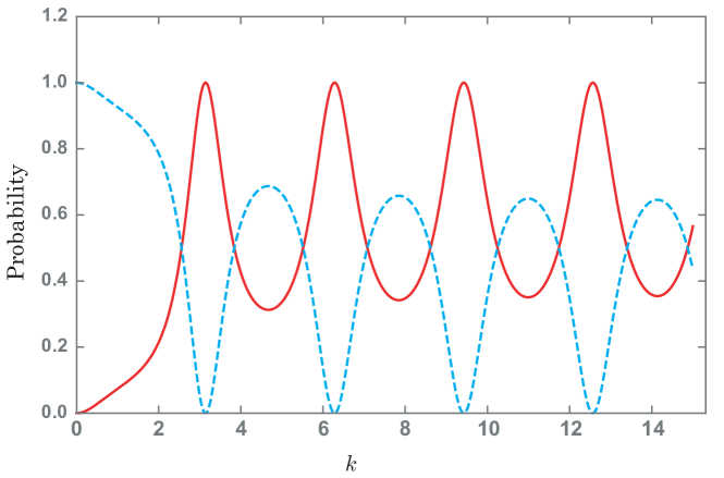
Figure 4: Probabilities vs $k$ in the case of $\alpha=\gamma=a=0$, $\beta=\delta=b=\frac{\pi}{4}$, $L_{(1)}=0$, and $L_{(2)}=L_{(3)}=1$. Here we adopt $\xi_{\rm I}=1$ and $\xi_{\rm I\!I}=0$. The red solid curve denotes the transmission probability, and the blue dashed curve denotes the reflection probability.

5 Disturbance to the symmetric ring conditions

5.1 Formulation for magnetic effects

In this section, we investigate effects of disturbance to the symmetric ring. As a most typical example, we consider effects of external magnetic fields on the quantum states. When we consider a charged particle on the ring and an external magnetic flux penetrating the ring, we should replace the partial derivative $\partial_{x}$ with the covariant derivative $D_{x}:=\partial_{x}-i\frac{e}{\hbar c}A_{x}$, where $e$ is an electric charge, and $A_{x}$ denotes the vector potential of magnetic fields, in Eqs. (1), (6) and (7). Let us also assume non-vanishing magnetic flux confined inside the ring. Since magnetic field on the wires vanishes, the magnetic vector potential is provided by pure gauge. The wave function in the presence of the magnetic flux is given by [23]

$$\Phi_{i}^{\rm(M)}(x_{i}) = e^{i\frac{e}{\hbar c}\chi_{i}(x_{i})}\Phi_{i}(x_{i})\quad(i=1,2,3,4),$$ (91)

where $\Phi_{i}$ is the wave function in the absence of the magnetic flux, which is given by Eq. (16), and

$$\chi_{i}(x) := \int^{x}_{\eta_{i}}A_{i}dx_{i}\quad(i=1,2,3,4).$$ (92)

Here $A_{i}$ denotes the tangential component of three-dimensional vector potential $\bi{A}$ along the $x_{i}$ axis, and $\eta_{i}$ is an arbitrary constant. We now take

$$\eta_{1}=\eta_{2}=\eta_{3}=\xi_{\rm I},\quad\eta_{4}=\xi_{\rm I\!I}.$$ (93)

Then we have

$$\chi_{1}(\xi_{\rm I})=\chi_{2}(\xi_{\rm I})=\chi_{3}(\xi_{\rm I})=0,\quad\chi_{4}(\xi_{\rm I\!I})=0.$$ (94)

Under this assumption, we derive

$$\Psi^{\rm(M)}(\xi_{\rm I})=\Psi(\xi_{\rm I}),\quad\Psi^{\prime\rm(M)}(\xi_{\rm I})=\Psi^{\prime}(\xi_{\rm I}),$$ (95)

$$\Psi^{\rm(M)}(\xi_{\rm I\!I})=P^{\dagger}\Psi(\xi_{\rm I\!I}),\quad\Psi^{\prime\rm(M)}(\xi_{\rm I\!I})=P^{\dagger}\Psi^{\prime}(\xi_{\rm I\!I}),$$ (96)

where $\Psi$ and $\Psi^{\prime}$ are given by Eqs. (17) and (18), and we define

$$P:={\rm diag}\left(e^{-i\frac{e}{\hbar c}\chi_{2}(\xi_{\rm I\!I})},e^{-i\frac{e}{\hbar c}\chi_{3}(\xi_{\rm I\!I})},1\right).$$ (97)

Hence the junction conditions in the presence of the magnetic flux are replaced with

$$(U-I_{3})\Psi(\xi_{\rm I})+iL_{0}(U+I_{3})\Psi^{\prime}(\xi_{\rm I})=0,$$ (98)

$$(PUP^{\dagger}-I_{3})\Psi(\xi_{\rm I\!I})+iL_{0}(PUP^{\dagger}+I_{3})\Psi^{\prime}(\xi_{\rm I\!I})=0.$$ (99)

Since $PUP^{\dagger}=P\tilde{V}\tilde{D}(P\tilde{V})^{\dagger}$ at the node II, the effect of the magnetic flux is expressed by

$$\tilde{V}\longrightarrow\tilde{V}^{(\rm M)}=P\tilde{V}.$$ (100)

Note that the magnetic flux $\phi_{0}$ penetrating the ring is given by

$$\phi_{0}=\chi_{3}(\xi_{\rm I\!I})-\chi_{2}(\xi_{\rm I\!I})=\oint_{\rm Ring}\bi{A}\cdot d\bi{r}.$$ (101)

When we consider a symmetric configuration for the ring arms, we have

$$\chi_{3}(\xi_{\rm I\!I})=-\chi_{2}(\xi_{\rm I\!I}).$$ (102)

Then we derive

$$\chi_{2}(\xi_{\rm I\!I})=-\frac{1}{2}\phi_{0},\quad\chi_{3}(\xi_{\rm I\!I})=\frac{1}{2}\phi_{0}.$$ (103)

Hence we obtain

$$P:={\rm diag}\left(e^{i\frac{e\phi_{0}}{2\hbar c}},e^{-i\frac{e\phi_{0}}{2\hbar c}},1\right).$$ (104)

This expression leads to

$$\tilde{V}\longrightarrow\tilde{V}^{(\rm M)} = P\tilde{V}$$ (105)

$$= e^{i\tilde{\alpha}^{\rm(M)}\lambda_{3}}e^{i\tilde{\beta}\lambda_{2}}e^{i\tilde{\gamma}\lambda_{3}}e^{i\tilde{\delta}\lambda_{5}}e^{i\tilde{a}\lambda_{3}}e^{i\tilde{b}\lambda_{2}},$$

where

$$\tilde{\alpha}^{\rm(M)}:=\tilde{\alpha}+\frac{e\phi_{0}}{2\hbar c}.$$ (106)

Therefore, when we assume the symmetric configuration for the ring arms, the effect of the magnetic flux can be expressed by the modulation of the parameter $\tilde{\alpha}$.

5.2 Effects of the magnetic disturbance on the transmission probability

We investigate the effects of the magnetic disturbance on the transmission probability. For the symmetric ring systems which the magnetic flux penetrates, the scattering matrix at the node II becomes

$$S_{\rm I\!I}=e^{2ik\left(\xi_{\rm I}-\xi_{\rm I\!I}\right)}e^{i\frac{e\phi_{0}}{2\hbar c}\lambda_{3}}S_{\rm I}^{\dagger}e^{-i\frac{e\phi_{0}}{2\hbar c}\lambda_{3}}.$$ (107)

From Eqs. (69) and (72), then we derive

$$R = \frac{1}{\Delta}\left[s_{11}\left(1-e^{2ik\left(\xi_{\rm I}-\xi_{\rm I\!I}\right)}\right)^{2}+2ie^{2ik\left(\xi_{\rm I}-\xi_{\rm I\!I}\right)}\sin\frac{e\phi_{0}}{2\hbar c}\right.$$ (108)

$$\times\left.\left\{e^{-i\frac{e\phi_{0}}{2\hbar c}}s_{23}^{\ast}\left(s_{11}s_{23}-s_{13}s_{21}\right)-e^{i\frac{e\phi_{0}}{2\hbar c}}s_{32}^{\ast}\left(s_{11}s_{32}-s_{12}s_{31}\right)\right\}\right]$$

$$T = \frac{e^{2ik\left(\xi_{\rm I}-\xi_{\rm I\!I}\right)}}{\Delta}\left[\left(1-|s_{11}|^{2}\right)\left(1-e^{2ik\left(\xi_{\rm I}-\xi_{\rm I\!I}\right)}\right)\left(1+2ie^{i\frac{e\phi_{0}}{4\hbar c}}\sin\frac{e\phi_{0}}{4\hbar c}\right)\right.$$ (109)

$$\left.-2i\sin\frac{e\phi_{0}}{2\hbar c}\left(|s_{21}|^{2}-e^{2ik\left(\xi_{\rm I}-\xi_{\rm I\!I}\right)}|s_{12}|^{2}\right)\right],$$

where

$$\Delta = \left(1-e^{2ik\left(\xi_{\rm I}-\xi_{\rm I\!I}\right)}|s_{11}|^{2}\right)\left(1-e^{2ik\left(\xi_{\rm I}-\xi_{\rm I\!I}\right)}\right)$$ (110)

$$+2ie^{2ik\left(\xi_{\rm I}-\xi_{\rm I\!I}\right)}\sin\frac{e\phi_{0}}{2\hbar c}\left(e^{-i\frac{e\phi_{0}}{2\hbar c}}|s_{23}|^{2}-e^{i\frac{e\phi_{0}}{2\hbar c}}|s_{32}|^{2}\right).$$

In the limit of vanishing magnetic flux, i.e., $\phi_{0}\rightarrow 0$, we retrieve the results in Eqs. (89) and (90). Equations (108) and (109) provide the general expressions of the amplitudes for the reflection and transmission in the symmetric ring system which magnetic flux penetrates. Note that $s_{ij}$ in the above equations are functions of the nine parameters of the Y-junction.

For example, if we adopt the following parameters

$$\alpha=\gamma=a=0,\quad\beta=\delta=b=\frac{\pi}{4},\quad L_{(1)}=L_{(2)}=0,\quad L_{(3)}\rightarrow\infty$$ (111)

then Eqs. (108) and (109) are reduced to

$$R = -\frac{e^{2ik\xi_{\rm I}}e^{2ik\left(\xi_{\rm I}-\xi_{\rm I\!I}\right)}\left(e^{-\frac{ie\phi_{0}}{\hbar c}}-1\right)^{2}}{e^{2ik\left(\xi_{\rm I}-\xi_{\rm I\!I}\right)}\left(e^{-\frac{ie\phi_{0}}{\hbar c}}+1\right)^{2}-4e^{-\frac{ie\phi_{0}}{\hbar c}}},$$ (112)

$$T = \frac{2e^{2ik\left(\xi_{\rm I}-\xi_{\rm I\!I}\right)}e^{-\frac{ie\phi_{0}}{2\hbar c}}\left(e^{2ik\left(\xi_{\rm I}-\xi_{\rm I\!I}\right)}-1\right)\left(e^{-\frac{ie\phi_{0}}{\hbar c}}+1\right)}{e^{2ik\left(\xi_{\rm I}-\xi_{\rm I\!I}\right)}\left(e^{-\frac{ie\phi_{0}}{\hbar c}}+1\right)^{2}-4e^{-\frac{ie\phi_{0}}{\hbar c}}}.$$ (113)

In this case, while when $\displaystyle\frac{e\phi_{0}}{\hbar c}=2n\pi$ ($n=0,1,2,\cdots$), we have $R=0$, when $\displaystyle\frac{e\phi_{0}}{\hbar c}=(2n+1)\pi$, we have $T=0$ for every mode characterized by a wavenumber. In Fig. 5, we show the transmission and reflection probabilities as a function of the wavenumber $k$ in the cases of (a) $\frac{e\phi_{0}}{\hbar c}=0$, (b) $\frac{e\phi_{0}}{\hbar c}=\frac{\pi}{2}$, and (c) $\frac{e\phi_{0}}{\hbar c}=\pi$. Furthermore, Fig. 6 shows the transmission probability as a function of the magnetic flux when $k=\frac{\pi}{2}$. Thus, the perfect transmission and the perfect reflection appear alternatively for every mode, as the strength of the magnetic flux increases. Similar results may occur in a subclass in the parameter space in which $s_{11}=0$. (see Eqs. (89) and (90)). Consequently, in this choice of parameters for the symmetric ring system, the modulation of the magnetic flux enable us to switch the current.

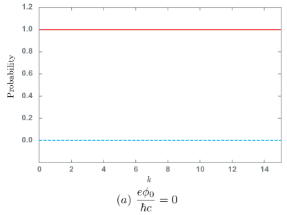
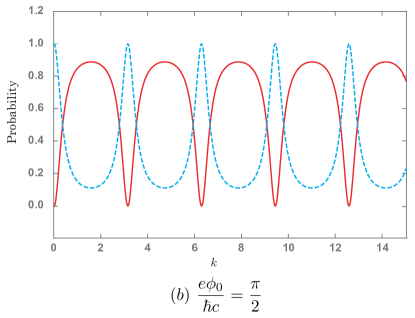
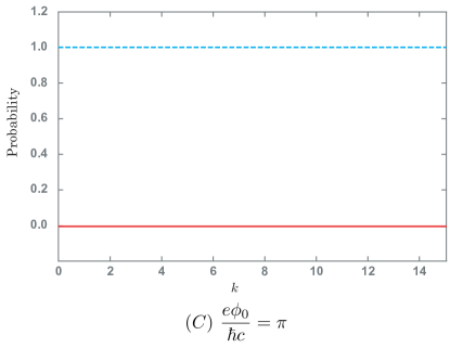
Figure 5: Probabilities vs $k$ in the cases of (a) $\frac{e\phi_{0}}{\hbar c}=0$, (b) $\frac{e\phi_{0}}{\hbar c}=\frac{\pi}{2}$, and (c) $\frac{e\phi_{0}}{\hbar c}=\pi$. Here we adopt $\alpha=\gamma=a=0$, $\beta=\delta=b=\frac{\pi}{4}$, $L_{(1)}=L_{(2)}=0$, $L_{(3)}=\infty$, $\xi_{\rm I}=1$ and $\xi_{\rm I\!I}=0$. The red solid curve denotes the transmission probability, and the blue dashed curve denotes the reflection probability. Note that when $\frac{e\phi_{0}}{\hbar c}=2n\pi$ ($n$ is an integer), we regain the same result as in the case of $\frac{e\phi_{0}}{\hbar c}=0$.

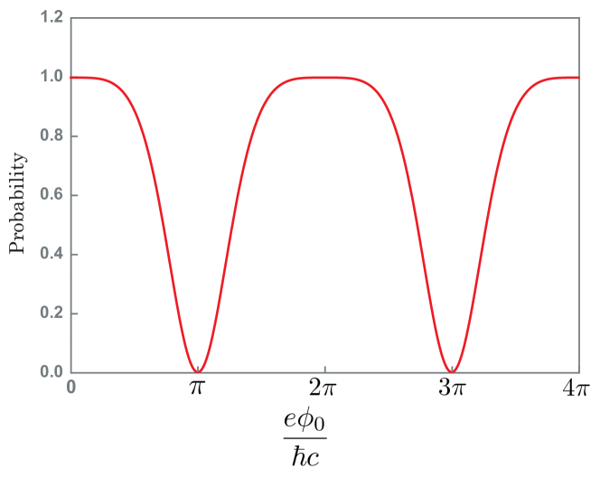
Figure 6: Transmission probabilities vs magnetic flux when $k=\frac{\pi}{2}$. Here we adopt the same parameters in Fig. 5.

Finally, we comment on the previous work [24]. In [24], the authors discussed conductance, which is connected to transmission probability via the Landauer formula, in a similar ring system composed of one-dimensional lattice using a tight-binding model. Although we have considered smooth one-dimensional wires, they considered the realistic lattice, whose system has a dispersion relation different from that of a free particle. However, when all the hopping integrals in [24] are taken to be 1 as in [24], their system would correspond to a limited class of symmetric ring systems in which $s_{11}=s_{22}=s_{33}$ and $s_{12}=s_{21}=s_{13}=s_{31}=s_{23}=s_{32}$ in our model. Thus our model deals with a very large class of junction conditions.

6 Conclusion

We have discussed quantum dynamics in the quantum ring systems with double Y-junctions in which two arms have same length. For these systems, a general formulation by scattering matrices was found to be useful. Based on our formulations, we investigated localized states on the ring. Then we found that the symmetric ring systems in which one node has the same parameters as the other node under the reflectional symmetry possess the following interesting features. In the symmetric ring systems, localized states exist inevitably, and resonant perfect transmission occurs when the wavenumber of an incoming wave coincides with that of the localized states, for any parameters of the nodes except for the extremal cases in which the absolute values of components of scattering matrices take $1$. We also investigated the external disturbance to the symmetric ring systems. In particular, we have considered the magnetic flux penetrating the ring. Then we found that the current through the symmetric ring system for every mode characterized by a wavenumber can be switched simultaneously by the strength of the magnetic flux only when we adopt a subclass of parameters for the Y-junctions.

We should briefly mention the time-reversal symmetry, which is a physically important class of problem, in the symmetric ring systems. The time-reversal symmetry of the ring systems requires that the matrix $S_{\rm R}$ given by Eqs. (40)-(49) be symmetric. In the symmetric rings, using Eqs. (75)-(78), we can show that $(S_{\rm R})_{12}=(S_{\rm R})_{21}$ from straightforward calculations. Thus the time-reversal symmetry always holds in the symmetric ring systems.

In this paper, we did not deal with anti-symmetric rings, which were considered in the previous work [21], and other cases in detail. Once we take a configuration which slightly deviates from the symmetric ring, numerous variations in the curves for transmission probabilities occur due to the vast parameter space for the Y-junctions. These would be investigated in the future works. More general discussion on magnetic field effects would also be provided.

References

• [1] Y. Aharonov and D. Bohm, 1959 Phys. Rev.115, 485
• [2] Y. Aharonov and A. Casher, 1984 Phys. Rev. Lett.53, 319
• [3] R. A. Webb, S. Washburn, C. P. Umbach, and R. B. Laibowitz, 1985 Phys. Rev. Lett.54, 2696
• [4] Akira Tonomura, Nobuyuki Osakabe, Tsuyoshi Matsuda, 1986 Takeshi Kawasaki, and Junji Endo, Phys. Rev. Lett.56, 792
• [5] A. Fuhrer, S. Lüscher, T. Ihn, T. Heinzel, K. Ensslin, W. Wegscheider and M. Bichler 2001 Nature 413, 822
• [6] S.Viefers, P. Koskinen, P. Singha Deo and M.Manninen 2004 Physica E 21, 1
• [7] T. Ihn, A. Fuhrer, L. Meier, M. Sigrist and K. Ensslin 2005 Europhysics News 36, 78
• [8] E. Räsänen, A. Castro, J. Werschnik, A. Rubio, and E. K. U. Gross 2007 Phys. Rev. Lett.98, 157404
• [9] E. Zipper, M. Kurpas, J. Sadowski, M. M. Maska, 2011 J. Phys.: Condens. Matter23, 115302
• [10] M. Büttiker, Y. Imry, and M. Ya. Azbel, 1984 Phys. Rev. B 30, 1982
• [11] M. Büttiker, 1985 Phys. Rev. B 32, 1846
• [12] M. Reed and B. Simon, 1980 Methods of Modern Mathematical Physics, Vol. II (Academic Press, New York)
• [13] P. Šeba, 1986 Czeck. J. Phys. 36 667
• [14] S. Albeverio, F. Gesztesy, R. Høegh-Krohn, and H. Holden, 1988 Solvable Models in Quantum Mechanics (Springer, New York)
• [15] T. Cheon, T. Fülöp, and I. Tsutsui, 2001 Ann. Phys. 294, 1
• [16] T. Cheon, P. Exner, and O. Turek 2009 J. Phys. Soc. Japan78, 124004
• [17] C. Texier and G. Montambaux, 2001 J. Phys. A: Math. Gen.34, 10307
• [18] S. Ami and C. Joachim, 2002 Phys. Rev. B 65, 155419
• [19] S. Ohya, 2012 Ann. Phys. 327, 1668
• [20] O. Turek and T. Cheon, 2012 Europhys. Lett. 98, 50005
• [21] Y. Fujimoto, K. Konno, T. Nagasawa, and R. Takahashi, 2020 \jpa53, 155302
• [22] S. Xu, W.-J. Gong, H. Z. Shen, and X. X. Yi, New J. Phys.23, 073027
• [23] L. D. Landau and E. M. Lifshitz, 1965 Quantum Mechanics Non-relativistic Theory Second (revised) edition (Pergamon Press, Oxford)
• [24] B. A. Z. Antonio, A. A. Lopes, and R. G. Dias, 2013 Eur. J. Phys.34, 831