Acceleration of Cooperative Least Mean Square via Chebyshev Periodical Successive Over-Relaxation

Abstract

A distributed algorithm for least mean square (LMS) can be used in distributed signal estimation and in distributed training for multivariate regression models. The convergence speed of an algorithm is a critical factor because a faster algorithm requires less communications overhead and it results in a narrower network bandwidth. The goal of this paper is to present that use of Chebyshev periodical successive over-relaxation (PSOR) can accelerate distributed LMS algorithms in a naturally manner. The basic idea of Chbyshev PSOR is to introduce index-dependent PSOR factors that control the spectral radius of a matrix governing the convergence behavior of the modified fixed-point iteration. Accelerations of convergence speed are empirically confirmed in a wide range of networks, such as known small graphs (e.g., Karate graph), and random graphs, such as Erdös-Rényi (ER) random graphs and Barabási-Albert random graphs.

I Introduction

It is expected that a massive number of terminals will be connected in networks using beyond 5G/6G standards. In such a situation, cooperative signal processing with neighboring nodes becomes more significant for enhancing the performance of signal processing regarding wireless communications. For example, assume a case of a massive MIMO detection. If base stations are allowed to exchange certain information among the neighboring base stations, there are opportunities to improve the detection performance as if virtual multiple receive antennas were composed. When a number of sensors are trying to learn a common multivariate regression model based on own local data, a distributed algorithm for the least mean square (LMS) may be a natural choice as a learning strategy.

In the field of machine learning, federated learning [Bonawitz], which is commonly implemented as a distributed algorithm with a centralized parameter server, is becoming a hot research topic. Fully distributed algorithms such as the average consensus algorithm [Xiao], which has no centralized server, have several advantages over the centralized distributed algorithms. One of the advantages is robustness, that is, even when some of nodes stop operating because of a malfunction or dead battery, a fully distributed algorithm often can keep working. Another merit of fully distributed algorithms is that it can balance signal traffics over a network. A centralized distributed algorithm often creates unbalanced network traffics, where the edges connected to the centralized server needs to accommodate the largest amount of traffics, and traffics on other edges in the network is much smaller than the traffic at the centralized server.

Diffusion LMS [Cattivelli, Sayed, Lopes] is a notable example of fully distributed estimation algorithm. The core of the diffusion LMS consists of two steps. The first step can be seen as a local LMS estimation and the second step is to diffuse the local estimations to neighboring nodes. All the agents in the network repeatedly execute these two steps and eventually all the agent states converges to the global solution. Sayed et al. [Sayed] reported an analysis of the convergence rate of diffusion LMS, and showed advantages both in stability and convergence rate. An acceleration method for Diffusion LMS based on belief propagation was discussed in [nakai]. A consensus-based distributed LMS algorithm was presented by Schizas et al. [Schizas]. Their derivation of the algorithm introduced auxiliary local variables for each agent and provided a global objective function that naturally fits the problem setting. The minimization problem for the global objective function can be cast as a convex constrained minimization problem. The proposed algorithm in [Schizas] is naturally derived from the ADMM formulation for solving the convex problem. Decentralized baseband signal processing of MIMO detection was discussed by Li et al. [Li]. MIMO signal detection is closely related to LMS problems. Decentralized baseband signal processing appears promising for reducing the prohibitive complexity of handling baseband signal processing with a massive number of antennas.

The authors proposed a method to accelerate the convergence of a fixed-point iteration in [takabe20]. The acceleration method is called Chebyshev periodical successive over-relaxation (Chbyshev PSOR), and it is applicable both to linear and non-linear fixed-point iterations. The basic idea of Chbyshev PSOR is to introduce index-dependent PSOR factors that control the spectral radius of a matrix governing the convergence behavior of the modified fixed-point iteration. The name of the method is named after the Chebyshev polynomials that are used for determining the PSOR factors. In [takabe20], it is shown that many fixed-point iterations, such as the Jacobi method for solving linear equations are successfully accelerated.

It would be very natural to use Chebyshev PSOR for accelerating a distributed LMS algorithm because most of a fully distributed LMS algorithm can be regarded as linear fixed-point iterations. Acceleration of a fully distributed LMS algorithm in convergence seems an appropriate problem to pursue because a fast algorithm generates less signal traffics over a network and it reduces computational complexity for each nodes.

The goal of this paper is to show that the use of Chebyshev-PSOR can accelerate distributed LMS algorithms in a naturally manner. We thus place our main focus on how to accelerate a fully distributed LMS algorithm, which is referred to as cooperative LMS. The cooperative LMS which is derived from the global objective function via the use of a proximal gradient method [Prox]. Our intension is not to develop the fastest algorithm but to present the principle for accelerating the convergence of a distributed LMS algorithm. Chebyshev PSOR can be applied to another distributed LMS algorithms but we restrict our attention to the cooperative LMS to keep the discussion focused. Cooperative LMS is closely related to the diffusion LMS [Cattivelli, Sayed, Lopes] and other distributed LMS algorithms [Schizas]. It is expected that the results shown in this paper is applicable to these algorithms as well.

II Preliminaries

II-A Notation

The range of integers from $1$ to $N$ is represented as $[N]$. The closed real interval from $a$ to $b$ is denoted by $[a,b]$ and the open interval is denoted by $(a,b)$. Let $\bm{A}$ be an $n\times n$ real symmetric matrix. The notation $\lambda_{min}(\bm{A})$ and $\lambda_{max}(\bm{A})$ denote the minimum and maximum eigenvalues of $\bm{A}$, respectively. The notation $\rho(\bm{A})$ indicates the spectral radius of $\bm{A}$. The matrix $\bm{I}_{n}$ means the identity matrix of size $n\times n$. If the size is evident from the context, the identity matrix is simply denoted by $\bm{I}$. The operator $\otimes$ represents the Kronecker product.

II-B Problem setup

Let $G:=(V,E)$ be an undirected connected graph representing a network of agents. Assume that an agent $k\in V:=\{1,2,\ldots,K\}$ can communicate with its neighboring agents in ${\cal N}(k):=\{j\mid(k,j)\in E\}$. Each agent has own observation vector $\bm{y}_{k}\in\mathbb{R}^{m}(m<N)$ which is given by $\bm{y}_{k}=\bm{H}_{k}\bm{x}^{0}+\bm{w}_{k}$ where $\bm{x}^{0}\in\mathbb{R}^{N}$ is a parameter vector unknown to all agents and $\bm{H}_{k}\in\mathbb{R}^{m\times N}$ is a real matrix known to agent $k$. The additive term $\bm{w}_{k}$ represents i.i.d. Gaussian noise vector where each component follows Gaussian distribution with zero mean and variance $\sigma^{2}$. To estimate the hidden global parameter $\bm{x}^{0}$, we can use the LMS estimation defined as $\bm{x}^{*}:=\text{argmin}_{\bm{x}\in\mathbb{R}^{N}}\sum_{k=1}^{K}(1/2)\|\bm{y}_{k}-\bm{H}_{k}\bm{x}\|^{2}.$ In the distributed environment defined above, it is natural to employ a gradient descent method to solve the LMS problem.

II-C Brief review of Chebyshev PSOR

In this subsection, we will briefly review some basic facts regarding Chebyshev PSOR according to [takabe20].

Let us consider the following linear fixed-point iteration:

$$\bm{x}^{(k+1)}:=\bm{A}\bm{x}^{(k)},\ k=0,1,2,\ldots$$ (1)

where $\bm{A}\in\mathbb{R}^{n\times n}$ and $\bm{x}^{(t)}\in\mathbb{R}^{n}$ for $k=0,1,2,\ldots$ as an example. The method in [takabe20] handles more general fixed-point iterations, such as $\bm{x}^{(k+1)}:=f(\bm{x}^{(k)})$ but we here restrict our attention to the simplest case required for the following discussion. If the spectral radius of $\bm{A}$ satisfies $\rho(\bm{A})<1$, the linear fixed-point iteration converges to the fixed point $\bm{x}^{*}=\bm{0}$.

Successive over-relaxation (SOR) is a well-known method for accelerating this fixed point iteration with the modified fixed point iteration:

$$\bm{x}^{(k+1)} :=\bm{x}^{(k)}+\omega_{k}\left(\bm{A}\bm{x}^{(k)}-\bm{x}^{(k)}\right),$$ (2)

where $\omega_{k}(k=0,1,\ldots)$ is a positive real number called a SOR factor. In this paper, we will use periodical SOR (PSOR) factors $\{\omega_{k}\}_{k=0}^{T-1}$ satisfying $\omega_{\ell T+j}=\omega_{j}\quad(\ell=0,1,2,\ldots,\ j=0,1,2,\ldots,T-1),$ where $T$ is a positive integer called the period of the PSOR factors. SOR using PSOR factors is referred to as a PSOR. The PSOR iteration (2) can be rewritten in a linear update form:

$$\bm{x}^{(k+1)}:=(\bm{I}-\omega_{k}\bm{B})\bm{x}^{(k)},$$ (3)

where the matrix $\bm{B}$ is defined by $\bm{B}:=\bm{I}-\bm{A}$. By using the periodicity of $\omega_{k}$, we immediately have an update equation for every $T$ iterations as

$$\bm{x}^{((\ell+1)T)} =\left[\prod_{k=0}^{T-1}(\bm{I}-\omega_{k}\bm{B})\right]\bm{x}^{(\ell T)}$$ (4)

$$=\bm{U}(\{\omega_{k}\}_{k=0}^{T-1})\bm{x}^{(\ell T)},$$ (5)

where $\bm{U}(\{\omega_{k}\}_{k=0}^{T-1}):=\prod_{k=0}^{T-1}(\bm{I}-\omega_{k}\bm{B})$. From this equation, we can observe that the dynamics of the linear update (4) is governed by the eigenvalues of $\bm{U}(\{\omega_{k}\}_{k=0}^{T-1})$ and we can control the PSOR coefficients $\{\omega_{k}\}_{k=0}^{T-1}$ to accelerate the convergence of (4). To find a suboptimal set of $\omega_{k}$, the polynomial defined by

$$\beta(\lambda;\{\omega_{k}\}_{k=0}^{T-1})=\left[\prod_{k=0}^{T-1}(1-\omega_{k}\lambda)\right]$$ (6)

is a useful tool. Let $\lambda_{1}\leq\lambda_{2}\leq\cdots\leq\lambda_{n}$ be the eigenvalues of $\bm{B}$. It is known that the eigenvalues of $\bm{U}(\{\omega_{k}\}_{k=0}^{T-1})$ can be represented as

$$\{\beta(\lambda_{1};\{\omega_{k}\}_{k=0}^{T-1}),\beta(\lambda_{2};\{\omega_{k}\}_{k=0}^{T-1})\ldots,\beta(\lambda_{n};\{\omega_{k}\}_{k=0}^{T-1})\}.$$

This fact inspires us to choose a polynomial with small absolute value in the range $[\lambda_{1},\lambda_{n}]$ to determine the PSOR factors $\{\omega_{k}\}_{k=0}^{T-1}$ because smaller absolute values of eigenvalues $\bm{U}(\{\omega_{k}\}_{k=0}^{T-1})$ lead to faster convergence.

The paper [takabe20] introduced an affine translate of the Chebyshev polynomial having the desired properties. We define the Chebyshev PSOR factors $\{\omega_{k}^{ch}\}_{k=0}^{T-1}$ for the range $[a,b]$ by

$$\omega_{k}^{ch}:=\left[\frac{b+a}{2}+\frac{b-a}{2}\cos\left(\frac{2k+1}{2T}\pi\right)\right]^{-1},$$ (7)

which are reciprocals of the roots of an affine translated Chebyshev polynomial. It is shown in [takabe20] that the polynomial defined by the Chebyshev PSOR factors $\beta(\lambda;\{\omega_{k}^{ch}\}_{k=0}^{T-1})$ has tightly bounded absolute values in the range $[a,b]$. Figure 1 displays the absolute value of $\beta(\lambda;\{\omega_{k}^{ch}\}_{k=0}^{T-1})$ for $T=1,2,4,8$ under the setting $a=0.1$ and $b=1.0$. We can readily confirm that the absolute values of the function in the range $[0.1,1.0]$ are tightly bounded.

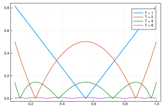
Figure 1: Plot of the absolute values of $\beta(\lambda;\{\omega_{k}^{ch}\}_{k=0}^{T-1})$ for $T=1,2,4,8$. The hyperparameters are set to $a=0.1$ and $b=1.0$.

III Derivation of Cooperative LMS Algorithm

III-A Distributed LMS problem as a regularization problem

Let $\bm{x}_{k}(k\in[K])$ be a state vector corresponding to the agent $k$, which represents a tentative estimate of $\bm{x}_{0}$. We here introduce a global loss function as

$$\ell(\bm{\chi}):=\frac{1}{2}\sum_{k\in[K]}\|\bm{y}_{k}-\bm{H}_{k}\bm{x}_{k}\|^{2}+\eta\bm{\chi}^{T}(\bm{L}\otimes\bm{I}_{N})\bm{\chi},$$ (8)

where the global state vector $\bm{\chi}$ is defined by

$$\bm{\chi}:=\left(\begin{array}[]{c}\bm{x}_{1}\\ \vdots\\ \bm{x}_{K}\\ \end{array}\right).$$ (9)

The matrix $\bm{L}:=\bm{D}-\bm{A}$ is the graph Laplacian of $G$ where $\bm{A}$ is the adjacency matrix of $G$ and $\bm{D}$ is the degree matrix of $G$, that is, the $(i,i)$ element of the diagonal matrix $\bm{D}$ is the degree of node $i$. It should be noted that

$$\bm{\chi}^{T}(\bm{L}\otimes\bm{I}_{N})\bm{\chi}=\frac{1}{2}\sum_{(i,j)\in E}\|\bm{x}_{i}-\bm{x}_{j}\|^{2}$$ (10)

holds, and it can be considered as a regularization term enforcing the proximity of neighboring agent states $\bm{x}_{i},\bm{x}_{j}((i,j)\in E)$. It is important to realize that the original LMS estimation and the minimizer $\bm{\chi}^{*}:=\text{argmin}_{\bm{\chi}\in\mathbb{R}^{KN}}\ell(\bm{\chi})$ are closely related but their solution may not be the same. The LMS estimation defined by the global loss function is denote by the cooperative LMS estimation. The problem for minimizing the global loss function is a quadratic problem and it is strictly convex if certain conditions are satisfied. In such a case, the minimization problem for $\ell(\bm{\chi})$ has a unique minimizer.

To solve the minimization problem regarding cooperative LMS, we will employ the proximal gradient method [Prox]. The gradient descent step is simply given by the following update rule:

$$\bm{\chi}^{(t+1)}:=\bm{\chi}^{(t)}-\mu\nabla_{\bm{\chi}}\frac{1}{2}\sum_{k\in[K]}\|\bm{y}_{k}-\bm{H}_{k}\bm{x}_{k}\|^{2}.$$ (11)

The proximal step can be approximated with a gradient descent step for the quadratic form $\eta\bm{\chi}^{T}(\bm{L}\otimes\bm{I}_{N})\bm{\chi}$, which can be given by $\bm{\chi}^{(t+1)}:=(\bm{I}-\eta\bm{L}\otimes\bm{I}_{N})\bm{\chi}^{(t)}.$ In the following subsections, we will discuss both steps in detail.

III-B Gradient descent step

Assume that $\bm{x}_{k}^{(t)}$ is the state of agent $k$ at discrete time index $t$. The gradient step (11) can be executed in parallel as

$$\bm{x}_{k}^{(t+1)} := \bm{x}_{k}^{(t)}+\mu\bm{H}_{k}^{T}(\bm{y}_{k}-\bm{H}_{k}\bm{x}_{k}^{(t)})$$ (12)

$$= (\bm{I}-\mu\bm{H}_{k}^{T}\bm{H}_{k})\bm{x}_{k}^{(t)}+\mu\bm{H}_{k}^{T}\bm{y}_{k}$$ (13)

$$= \bm{A}_{k}\bm{x}_{k}^{(t)}+\bm{b}_{k},$$ (14)

where $\bm{A}_{k}:=\bm{I}-\mu\bm{H}_{k}^{T}\bm{H}_{k}$ and $\bm{b}_{k}=\mu\bm{H}_{k}^{T}\bm{y}_{k}$. The global state vector $\bm{\chi}^{(t)}$ at time index $t$ and the offset vector $\bm{\beta}$ are defined by

$$\bm{\chi}^{(t)}:=\left(\begin{array}[]{c}\bm{x}_{1}^{(t)}\\ \bm{x}_{2}^{(t)}\\ \vdots\\ \bm{x}_{K}^{(t)}\\ \end{array}\right),\quad\bm{\beta}:=\left(\begin{array}[]{c}\bm{b}_{1}\\ \bm{b}_{2}\\ \vdots\\ \bm{b}_{K}\\ \end{array}\right).$$ (15)

Let $\bm{D}\in\mathbb{R}^{NK\times NK}$ be a block diagonal matrix consisting of $\bm{A}_{1},\ldots,\bm{A}_{K}$ as diagonal block matrices:

$$\bm{D}:=\left(\begin{array}[]{cccc}\bm{A}_{1}&&&\\ &\bm{A}_{2}&&\\ &&\ddots&\\ &&&\bm{A}_{k}\\ \end{array}\right).$$ (16)

From these notation, we can compactly represent the gradient descent step as $\bm{\chi}^{(t+1)}:=\bm{D}\bm{\chi}^{(t)}+\bm{\beta}.$

III-C Average consensus protocol as proximal step

Next, we consider an implementation of the proximal step. We here introduce the simplest average consensus scheme based on the update equation:

$$\bm{x}_{k}^{(t+1)}:=\bm{x}_{k}^{(t)}+\eta\sum_{j\in{\cal N}(k)}(\bm{x}_{j}^{(t)}-\bm{x}_{k}^{(t)}),$$ (17)

where $\eta$ is a positive real number. If the parameter $\eta$ is appropriately determined, the above iterations eventually converge to the average of the initial vectors. The process is known as average consensus. A careful observation reveals that the consensus iteration defined by (17) can be represented by

$$\bm{\chi}^{(t+1)}:=(\bm{I}-\eta\bm{L}\otimes\bm{I}_{N})\bm{\chi}^{(t)},$$ (18)

which shows the equivalence between the proximal step defined above and the average consensus protocol (17).

IV Properties of Cooperative LMS Algorithm

In the previous section, we saw that the gradient descent step can be executed perfectly in parallel and that the proximal step can be executed with the average consensus protocol which only requires neighboring interactions between agents. In this section, we will study cooperative LMS which is a realization of the proximal gradient method.

IV-A Implementation of cooperative LMS algorithm

In this paper, we deal with the simple distributed LMS defined in Alg. IV-A, which can solve the cooperative LMS problem. This algorithm is closely related to diffusion LMS [Cattivelli, Sayed, Lopes] and consensus-based learning algorithms [Schizas].

Algorithm 1 Cooperative LMS

1:  For each $k\in[K]$, set $\bm{x}^{(0)}:=\bm{0}$

2:  for $t:=0$ to $L-1$ do

3:     for $k:=1$ to $K$ do

4:        u_k^(t) :=x_k^(t) + μH_k^T(y_k - H_k x_k^(t))$\lx@algorithmic@item@@[]\hskip 25.00003pt$x_k^(t+1) := u_k^(t) + η∑_j ∈N(k) (u_j^(t) - u_k^(t))$\lx@algorithmic@item@@[]\hskip 25.00003pt\textbf{end}\ \textbf{for}\lx@algorithmic@item@@[]\hskip 25.00003pt\textbf{end}\ \textbf{for}\lx@algorithmic@item@@[]\hskip 25.00003pt\textbf{return}{}\$x_1^(L), x_2^(L), …, x_K^(L) For the following analysis, it is desirable to have an equivalent algorithm that is based on the update equation for $\bm{\chi}^{(t)}$. Combining the two update rules, specifically, the gradient step and the proximal step, we immediately have the following global update rule corresponding to Alg. IV-A:

$$\bm{\chi}^{(t+1)} := (\bm{I}-\eta\bm{L}\otimes\bm{I}_{N})(\bm{D}\bm{\chi}^{(t)}+\bm{\beta})$$

$$= \bm{Q}\bm{\chi}^{(t)}+(\bm{I}-\eta\bm{L}\otimes\bm{I}_{N})\bm{\beta},$$

where $\bm{Q}:=(\bm{I}-\eta\bm{L}\otimes\bm{I}_{N})\bm{D}.$ An equivalent algorithm shown in Alg. 2 includes an affine fixed point iteration whose error dynamics of the system is governed by the matrix: $\bm{Q}:=(\bm{I}_{KN}-\eta\bm{L}\otimes\bm{I}_{N})\bm{D}.$ Algorithm 2 Cooperative LMS (equivalent form) 1:  $\bm{\chi}^{(0)}=\bm{0}$ 2:  for $t=0$ to $L-1$ do 3:     $\bm{\chi}^{(t+1)}=\bm{Q}\bm{\chi}^{(t)}+(\bm{I}_{KN}-\eta\bm{L}\otimes\bm{I}_{N})\bm{\beta}$ 4:  end for 5:  return  $\bm{\chi}^{(L)}$ Assume that the affine fixed-point iteration (4) has a fixed point $\bm{\chi}^{*}$ that satisfies

$$\bm{\chi}^{*}=(\bm{I}-\eta\bm{L}\otimes\bm{I}_{N})\bm{D}\bm{\chi}^{*}+(\bm{I}-\eta\bm{L}\otimes\bm{I}_{N})\bm{\beta}.$$ (20)

By subtracting the above equation from (4), we immediately obtain a fixed-point iteration representing the evolution of error:

$$\bm{\chi}^{(t+1)}-\bm{\chi}^{*}=\bm{Q}(\bm{\chi}^{(t)}-\bm{\chi}^{*}).$$ (21)

From this error evolution equation, we can prove the following inequality which indicates linear convergence of the cooperative LMS algorithm to the global minimum if $\lambda_{max}(\bm{D})<1$.

Lemma 1

If $\bm{Q}$ is positive definite, the following inequality holds: $\displaystyle\frac{\|\bm{\chi}^{(t+1)}-\bm{\chi}^{*}\|}{\|\bm{\chi}^{(t)}-\bm{\chi}^{*}\|}\leq\lambda_{max}(\bm{D}).$ (22) (Proof) By taking the norm of both sides of (21), we have

$$\|\bm{\chi}^{(t+1)}-\bm{\chi}^{*}\| =\|\bm{Q}(\bm{\chi}^{(t)}-\bm{\chi}^{*})\|$$ (23)

$$\leq\|(\bm{I}_{KN}-\eta\bm{L}\otimes\bm{I}_{N})\|\|\bm{D}\|\|\bm{\chi}^{(t)}-\bm{\chi}^{*}\|$$ (24)

$$=\|\bm{D}\|\|\bm{\chi}^{(t)}-\bm{\chi}^{*}\|$$ (25)

$$=\rho(\bm{D})\|\bm{\chi}^{(t)}-\bm{\chi}^{*}\|$$ (26)

$$=\lambda_{max}(\bm{D})\|\bm{\chi}^{(t)}-\bm{\chi}^{*}\|,$$ (27)

where the second inequality uses the fact $\|(\bm{I}_{KN}-\eta\bm{L}\otimes\bm{I}_{N})\|=1$.

IV-B Smallest and largest eigenvalues of $\bm{Q}$

The matrix $\bm{Q}$ should be positive definite so that the objective function (8) becomes strictly convex. Furthermore, the eigenvalues of $\bm{Q}$ are of critical importance because they determines the convergence behavior of Chebyshev PSOR. In the following, we discuss the positive definiteness of $\bm{Q}$. The following two lemmas will be basis of the positive definiteness of $\bm{Q}$.

Lemma 2

If $\eta<1/\lambda_{max}(\bm{L})$, then $\bm{I}_{KN}-\eta\bm{L}\otimes\bm{I}_{N}$ is positive definite. (Proof) Let $\bm{A},\bm{B}\in\mathbb{R}^{n\times n}$. It is known that the set of eigenvalues of $\bm{A}\otimes\bm{B}$ is given by $\{\lambda_{A}\lambda_{B}\mid\lambda_{A}\in\Lambda_{A},\lambda_{B}\in\Lambda_{B}\}$ where $\Lambda_{A}$ and $\Lambda_{B}$ is the set of eigenvalues of $\bm{A}$ and $\bm{B}$, respectively. The eigenvalues of $\eta\bm{L}\otimes\bm{I}_{N}$ is thus in the range $[\eta\lambda_{min}(\bm{L}),\eta\lambda_{max}(\bm{L})]$. Then, the minimum eigenvalue of $\bm{I}_{KN}-\eta\bm{L}\otimes\bm{I}_{N}$ becomes $1-\eta\lambda_{max}(\bm{L})$. Due to the assumption $\eta<1/\lambda_{max}(\bm{L})$, we have $\lambda_{min}(\bm{I}_{KN}-\eta\bm{L}\otimes\bm{I}_{N})>0$.

Lemma 3

If $\lambda_{max}(\bm{H}_{k}^{T}\bm{H}_{k})<1/\mu$ for all $k\in[K]$, then $\bm{D}$ is positive definite. (Proof) The claim is equivalent to the positive definiteness of all the matrices $\bm{I}-\mu\bm{H}_{k}^{T}\bm{H}_{k}$ under the condition $\lambda_{max}(\bm{H}_{k}^{T}\bm{H}_{k})<1/\mu$ for all $k\in[K]$. The minimum eigenvalue can be evaluated as $$\lambda_{min}(\bm{I}-\mu\bm{H}_{k}^{T}\bm{H}_{k})=1-\mu\lambda_{max}(\bm{H}_{k}^{T}\bm{H}_{k}).$$ (28) When the condition is met, we immediately have $\lambda_{min}(\bm{I}-\mu\bm{H}_{k}^{T}\bm{H}_{k})>0$ for any $k\in[K]$. The following theorem clarifies when $\bm{Q}$ is guaranteed to be positive definite.

Theorem 1

If $\eta<1/\lambda_{max}(\bm{L})$ and $\lambda_{max}(\bm{H}_{k}^{T}\bm{H}_{k})<1/\mu$ for all $k\in[K]$, $\bm{Q}$ is positive definite and all the eigenvalues of $\bm{Q}$ are real. (Proof) Assume that two Hermitian matrices $\bm{X},\bm{Y}$ are both positive definite. Then, $\bm{X}\bm{Y}$ is also positive definite and all the eigenvalues of $\bm{X}\bm{Y}$ are real. Under the given condition, $\bm{I}_{KN}-\eta\bm{L}\otimes\bm{I}_{N}$ and $\bm{D}$ are both hermitian and positive definite from above lemmas. The claim of the theorem follows from the above product property. We next examine the largest eigenvalue of $\bm{Q}$. If $\bm{Q}$ is positive definite, the largest eigenvalue of $\bm{Q}$ coincides with the spectral radius of $\bm{Q}$.

Theorem 2

If $\eta<1/\lambda_{max}(\bm{L})$ and $\lambda_{max}(\bm{H}_{k}^{T}\bm{H}_{k})<1/\mu$ for all $k\in[K]$, any eigenvalue of $\bm{Q}$ is in the range $(0,1)$. (Proof) We can upper bound the largest eigenvalue of $\bm{Q}$ in the following way: $\displaystyle\lambda_{max}(\bm{Q})$ $\displaystyle=\rho(\bm{Q})$ (29) $\displaystyle\leq\|\bm{Q}\|$ (30) $\displaystyle\leq\|(\bm{I}_{KN}-\eta\bm{L}\otimes\bm{I}_{N})\|\|\bm{D}\|$ (31) $\displaystyle=\max_{k=1}^{K}\lambda_{max}(\bm{I}_{N}-\mu\bm{H}_{k}^{T}\bm{H}_{k})$ (32) $\displaystyle=1-\mu\min_{k=1}^{K}\lambda_{min}(\bm{H}_{k}^{T}\bm{H}_{k})$ (33) $\displaystyle<1,$ (34) where the first inequality is due to the norm upper bound for the spectral radius. The second inequality is based on the sub-additivity of the operator norm. Since the laplacian $\bm{L}$ has zero eigenvalue, we have $\|(\bm{I}_{KN}-\eta\bm{L}\otimes\bm{I}_{N})\|=\rho(\bm{I}_{KN}-\eta\bm{L}\otimes\bm{I}_{N})=1$. Combining the claim of Theorem 1, we have the claim of this theorem. From the proof of this theorem, we get to know that $\displaystyle\lambda_{max}(\bm{D})<1$ (35) if $\eta<1/\lambda_{max}(\bm{L})$ and $\lambda_{max}(\bm{H}_{k}^{T}\bm{H}_{k})<1/\mu$ for all $k\in[K]$. In order to have the lowest $\lambda_{max}(\bm{D})$ to get the fastest convergence rate in (22), an optimal choice of the parameters would be $\displaystyle\eta$ $\displaystyle=\frac{1-\epsilon}{\lambda_{max}(\bm{L})},$ (36) $\displaystyle\mu$ $\displaystyle=\frac{1-\epsilon}{\max_{k=1}^{K}\lambda_{max}(\bm{H}_{k}^{T}\bm{H}_{k})}$ (37) where $\epsilon$ is a small positive real number. It is easy to confirm that these parameter setting satisfies the positive definiteness conditions on $\eta$ and $\mu$.

IV-C Validation of choice of $\eta$ and $\mu$

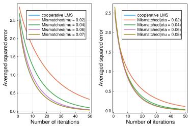
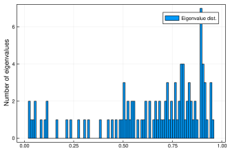
In this section, we will provide experimental validation for the choice of $\eta$ and $\mu$ given by (36) and (37) where we will confirm whether these parameter setting practically provides fast convergence or not. The experimental conditions are summarized as follows. We used Karate graph with $K=34$. The dimension of the $\bm{x}_{0}$ is set to $N=3$ where each element in $\bm{x}_{0}$ follows ${\cal N}(0,1)$. Each element in $H_{k}$ follows ${\cal N}(0,1)$ where $H_{k}\in\mathbb{R}^{2\times 3}$, i.e., $m=2$. The standard deviation of the observation noises is set to $\sigma=0.1$. The parameter $\epsilon$ used in (36) and (37) is set to $0.05$. In order to estimate the expectation, we run 100-trials. In the first experiment, while we fix the parameter $\eta$ as the value determined by (36), we use several mismatched values of $\mu$ in the cooperative LMS defined by Alg. IV-A. Namely, the ASE performance of mismatched LMS’s are examined here. Figure 2 (left) presents the ASEs as the function of the number of iterations. The ASE of the mismatched LMS with $\mu\in\{0.02,0.04,0.06,0.07\}$ are presented. As a baseline for comparison, ASE of the cooperative LMS with the parameter determined by (36) and (37) is also included in the figure. In this case, the average value of $\mu$ given by (37) is $0.0741$. We can immediately observe that the convergence becomes faster as $\mu$ approaches to $0.07$. Note that the parameter setting $\mu>0.9$ results in unstable behavior, i.e., the ASE is diverging in some cases. This experimental results provides a justification of the use of (37). Figure 2: Averaged squared errors of mismatched LMS: (left) fixed $\eta$ determined by (36), (right) fixed $\mu$ determined by (37). We then discuss a mismatched cooperative LMS with fixed $\mu$ determined by (37). The experimental conditions are exactly the same as the previous one. The only difference is that $\eta\in\{0.02,0.04,0.06,0.08\}$ is used with fixed $\mu$. Figure 2 (right) displays the ASE of the mismatched LMS with fixed $\mu$. We can see that convergence becomes faster as $\eta$ grows but almost no improvement can be obtained for $\eta>0.06$. In this case, the average value of $\eta$ defined by (36) is $0.05238$. This result implies that the value obtained by (36) seems near optimal with respect to $\eta$. In summary, from this experimental results, we can say that the parameter setting based on (36) and (37) are reasonable one to get sufficiently fast convergence of the cooperative LMS. Figure 3 shows an eigenvalue distribution of the matrix $\bm{Q}$ under the same parameter setting. We can confirm that all the eigenvalues of $\bm{Q}$ are included in the range $(0,1)$ which is consistent with the claim of Theorem 2. The parameters $\eta$ and $\mu$ are set to $\eta=0.0523,\mu=0.0688$ according to (36) and (37) in this case. Figure 3: Eigenvalue distribution of $\bm{Q}$ for Karate graph

IV-D Performance measure

After the cooperative LMS is executed, agent $k$ has its own estimate $\bm{x}_{k}^{(L)}$. In this paper, the quality of the estimation is evaluated by the averaged squared error defined by $\displaystyle E_{L}:=(1/K)\sum_{k=1}^{K}\|\bm{x}^{*}-\bm{x}_{k}^{(L)}\|^{2},$ (38) where $\bm{x}^{*}$ is the original LMS solution. If $\bm{H}_{k}(k\in[K])$ is stochastic, that is, randomly generated, the expectation $\mathbb{E}[E_{L}]$ will be estimated as the primary performance measure. For the benchmark purpose, noncooperative LMS for each agent, that is, $\bm{x}^{*}_{k}:=\text{argmin}_{\bm{x}\in\mathbb{R}^{N}}\frac{1}{2}\|\bm{y}_{k}-\bm{H}_{k}\bm{x}\|^{2},\ k\in[K]$ will be considered. In such a case, the average LMS for noncooperative LMS is given by $\tilde{E}_{L}=(1/K)\sum_{k=1}^{K}\|\bm{x}^{*}_{k}-\bm{x}_{k}^{(L)}\|^{2}.$

V Chebyshev PSOR for Cooperative LMS

It is natural to introducing Chebyshev-PSOR method to the cooperative LMS for accelerating the convergence speed. In this section, we will show Chebyshev-accelerated cooperative LMS.

V-A Chebyshev interval

The error evolution in (21) can be rewritten as $\bm{e}^{(t+1)}=\bm{Q}\bm{e}^{(t)}$ where $\bm{e}^{(t)}:=\bm{\chi}^{(t)}-\bm{\chi}^{*}$. It can be seen as a linear fixed-point iteration. When we apply PSOR to the cooperative LMS, the evolution can be described as $\displaystyle\bm{e}^{((\ell+1)T)}$ $\displaystyle=\left[\prod_{k=0}^{T-1}(\bm{I}-\omega_{k}\bm{B})\right]\bm{e}^{(\ell T)},$ (39) where $\bm{B}:=\bm{I}-\bm{Q}$. According to the strategy proposed in [takabe20], we can introduce Chebyshev PSOR factors for bounding the absolute values of eigenvalues of $\prod_{k=0}^{T-1}(\bm{I}-\omega_{k}\bm{B})$. To obtain the best convergence rate, [takabe20] proposed settings of $a=\lambda_{min}(\bm{I}-\bm{Q})$ and $b=\lambda_{max}(\bm{I}-\bm{Q})$. However, in this paper, we will treat $a$ and $b$ as hyperparameters that define the Chebyshev interval $[a,b]$. This is because the discussion in [takabe20] mainly considers the minimization of the spectral radius of $\prod_{k=0}^{T-1}(\bm{I}-\omega_{k}\bm{B})$ but the contributions of other eigenvalues to the error magnitude are not negligible when the number of iterations is small. Namely, for the cooperative LMS, an appropriate choice of the Chebyshev interval $[a,b]$ is important for obtaining a smaller error magnitude when the number of iterations is relatively small.

V-B Chebyshev cooperative LMS algorithm

Algorithm V-B shows the details of the Chebyshev cooperative LMS Algorithm. Lines 6-8 of the Chebyshev cooperative LMS algorithm represents corresponds to the additional PSOR process. The process in Line 8, $\displaystyle\bm{x}_{k}^{(t+1)}=(1-\omega)\bm{x}_{k}^{(t)}+\omega\bm{v}_{k}^{(t)}$ (40) combines the input with the gradient step and the output from the proximal step. This process can be carried out in each node in parallel. Because the Chebyshev-PSOR factor $\omega$ should be the same for every agent, the loop index $t$ is needed to be synchronized for all the agents. The additional computational complexity in Lines 6-8 is negligible compared with the required computational complexity required to execute Lines 4 and 5. Algorithm 3 Chebyshev cooperative LMS 1:  For each $k\in[K]$, set $\bm{x}^{(0)}:=\bm{0}$ 2:  for $t:=0$ to $L-1$ do 3:     for $k:=1$ to $K$ do 4:        u_k^(t) :=x_k^(t) + μH_k^T(y_k - H_k x_k^(t))$\lx@algorithmic@item@@[]\hskip 25.00003pt$v_k^(t) := u_k^(t) + η∑_j ∈N(k) (u_j^(t) - u_k^(t))$\lx@algorithmic@item@@[]\hskip 25.00003pt$t’ := t mod T$\lx@algorithmic@item@@[]\hskip 25.00003pt$ω:= [(b+a)/2 + ((b-a)/2) cos(π(2t’+1)/(2T)) ]^-1$\lx@algorithmic@item@@[]\hskip 25.00003pt$x_k^(t+1) := (1 - ω)x_k^(t) + ωv_k^(t) $\mathrm{missing-subexpression}$