Ground state properties and exact thermodynamics of a 2-leg anisotropic spin ladder system

Abstract

We study a frustrated two-leg spin ladder with alternate isotropic Heisenberg and Ising rung exchange interactions, whereas, interactions along legs and diagonals are Ising-type. All the interactions in the ladder are anti-ferromagnetic in nature and induce frustration in the system. This model shows four interesting quantum phases: (i) stripe rung ferromagnetic (SRFM), (ii) stripe rung ferromagnetic with edge singlet (SRFM-E), (iii) anisotropic antiferromagnetic (AAFM), and (iv) stripe leg ferromagnetic (SLFM) phase. We construct a quantum phase diagram for this model and show that in stripe rung ferromagnet (SRFM), the same type of sublattice spins (either $S$ or $\sigma$-type spins) are aligned in the same direction. Whereas, in anisotropic antiferromagnetic phase, both $S$ and $\sigma$-type of spins are anti-ferromagnetically aligned with each other, two nearest $S$ spins along the rung form an anisotropic singlet bond whereas two nearest $\sigma$ spins form an Ising bond. In large Heisenberg rung exchange interaction limit, spins on each leg are ferromagnetically aligned, but spins on different legs are anti-ferromagnetically aligned. The thermodynamic quantities like $Cv(T)$, $\chi(T)$ and $S(T)$ are also calculated using the transfer matrix method for different phase. The magnetic gap in the SRFM and the SLFM can be notice from $\chi(T)$ and $Cv(T)$ curves.

I Introduction

The study of quantum phase transitions in low dimensional spin systems has been a frontier area of research due to abundance of effective low-dimensional magnetic materials hutchings1979 ; park2007 ; mourigal2012 ; drechsler2007 ; dutton201224 ; dutton2012108 ; maeshima2003 ; sandvik1996 ; johnston1987 ; dagotto1996 which exhibits a zoo of phases okamoto1992 ; haldan1982 ; srwhite1996 ; chitra1995 ; mkumar2015 ; soos2016 ; ckm1969 ; shastry1981 ; srwhite1994 ; chubukov1991 ; furkawa2012 ; zhitomirsky2010 ; parvej2017 . The confinement and interplay of exchange interactions in low dimensional systems like spin chains heilmann1978 ; hutchings1979 ; umegaki2015 , spin ladders sandvik1996 ; johnston1996 ; barnes1993 ; dagotto1996 or two dimensional systems manousakis1991 ; singh2010 can give rise to various interesting ground state (GS) properties mourigal2011 ; enderle2010 ; seidov2017 ; mkumar2013 ; mkumar2016 ; sirker2010 ; hamada1988 . Recently synthesized materials show that many of these spin-1/2 systems are frustrated even in one dimension (1D) mourigal2012 ; dutton201224 ; park2007 ; drechsler2007 , whereas the low dimensional systems can be either geometrically frustrated i.e. antiferromagnet Heisenberg spin-1/2 on a triangular lattice anderson1973 ; fazekas1974 or exchange interaction driven frustration such as 1D spin-1/2 system interacting with nearest neighbor interaction $J_{1}$ and antiferromagnetic next nearest neighbor exchange interaction $J_{2}$ mg1969 ; srwhite1996 ; chitra1995 ; okamoto1992 ; mkumar2010 ; tonegawa1987 ; sebastian1996 . Frustrated model Hamiltonians of one dimensional systems and zigzag geometry Korotin1999 ; Korotin2000 are extensively studied theoretically and GS of these systems have exotic phases like spin liquid savary2017 ; dagotto1996 , dimer srwhite1996 ; chitra1995 ; mkumar2015 ; soos2016 ; ckm1969 ; shastry1981 ; srwhite1994 ; haldan1982 , spiral/non-collinear spin phase mkumar2015 ; soos2016 ; dmaiti2019 , ferromagnetic phase etc.

Spin chains and ladders can also have anisotropic exchange interactions curely1986 ; strecka2003 ; rezania2015 ; cizmar2010 ; thielemann2009 and some spin chains can have alternate Heisenberg and Ising exchange interactions rojas2016 , whereas exchange along the leg is Ising type. The Heisenberg-Ising model has been explored by few groups verkholayak2012 ; verkholayak2013 ; rojas2016 . The simplest model on a ladder geometry studied by Rojas et. al. rojas2016 with alternate anisotropic Heisenberg ($J_{x}$,$J_{x}$,$J_{z}$) and Ising type ($J_{0}$) rung exchanges and intraleg exchange interaction ($J_{1}$) gives interesting ground-state phase diagram with phases like frustrated phase 1 (FRU1), antiferromagnetic phase etc. in large and small ratio of Ising to Heisenberg exchange interactions ($J^{z}/J_{1}$) limits respectively. This model also shows interesting sharp peak in specific heat. Verkholyak et. al. verkholayak2013 studied an anisotropic model with Heisenberg rung exchange interaction ($J_{1}$) and Ising-type leg exchange interaction ($J_{2}$) and diagonal exchange interaction ($J_{3}$). They showed that GS can exhibit different phases e.g. stripe leg (SL), stripe rung (SR), Néel and quantum paramagnetic (QPM) phases etc. in the phase diagram of $J_{3}$-$J_{1}$ plane and the field dependence behavior in this model are also studied verkholayak2012 . There are other studies of Heisenberg branched chain model which show interesting GS behavior and plateau phase in the presence of external magnetic field karl2019 .

The thermodynamical properties of the one or quasi-one dimensional quantum spin models with alternating isotropic and anisotropic units are studied extensively in recent times rojas2016 ; sahoo2012 . In presence of alternate Heisenberg and Ising rung and Ising leg interaction, the two consecutive units of the Hamiltonian become commuting and in such cases, the exact thermodynamical properties of these systems can be calculated using transfer matrix method. For example, the susceptibility and other related quantities were calculated exactly for an anisotropic helical single-chain magnet $Fe_{2}Nb$ using transfer matrix method sahoo2012 .

In this paper, we study a general anisotropic Heisenberg-Ising model on ladder geometry with alternate Heisenberg and Ising exchange rung interactions, whereas the exchange interactions along the leg and along the diagonal of the ladder are Ising type as shown in Fig. 1. The system exhibits anisotropic antiferromagnetic (AAFM), stripe rung ferromagnetic (SRFM), stripe rung ferromagnetic-edge (SRFM-E) and stripe leg ferromagnetic (SLFM) phases. We use exact diagonalisation method to calculate the GS properties upto 24 sites using Davidson algorithm davidson1975 for diagonalisation of the Hamiltonian matrix, whereas the thermodynamical properties are studied using the transfer matrix method huangstat . The specific heat, magnetic susceptibility, entropy and average energy are studied in various phases.

This paper is divided into four sections, and in section II we discuss the model Hamiltonian. In section III results are discussed and is divided into four subsections. We summarise all the results and conclude in the section IV.

II Model Hamiltonian

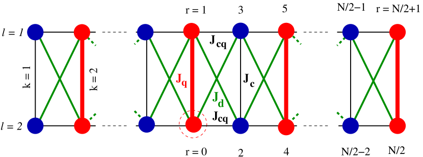
Figure 1: (Color online). Schematic model diagram for spin configurations of a 2-leg anisotropic spin ladder system with $N(=4n)$ sites is shown. The interactions along the odd and even rungs are Ising and Heisenberg type respectively. Both along the legs and diagonals, the interactions are Ising-type. The indices $k$ ($1\leq k\leq 2n$) and $l$ (= 1 or 2) in the figure represent the rung and leg number; any spin in the anisotropic or isotropic rung is denoted by $\sigma_{k,l}$ or $S_{k,l}$ respectively. The variable $r$ is the distance from the reference spin shown within a dotted circle.

We consider here a frustrated spin-1/2 ladder with alternating isotropic Heisenberg and Ising type interactions. For convenience, the system is divided into two sublattices A and B. The A sublattice has Heisenberg rung interaction $J_{q}$ while the B sublattice has Ising rung interaction $J_{c}$. The spins of two sublattices are connected by Ising-type interaction $J_{cq}$ along the legs and also by diagonal Ising-type interaction $J_{d}$. Since for the B sublattice, only the $z$-component of spins appear in the Hamiltonian, we represent these spins by $\sigma$, whereas the other spins $S$ have all three components. The schematic diagram of the spin model is shown in Fig. 1.

The Hamiltonian for this system (having $4n$ sites) with open boundary condition (OBC) is given by $\mathbf{H}=\sum_{i=1}^{n-1}\mathbf{H_{i}}+\mathbf{H_{e}}$ where,

$$\mathbf{H_{i}}=J_{q}\vec{S}_{2i,1}\cdot\vec{S}_{2i,2}+\frac{J_{c}}{2}(\sigma_{2i-1,1}\sigma_{2i-1,2}+\sigma_{2i+1,1}\sigma_{2i+1,2})$$

$$+J_{cq}\left\{S_{2i,1}^{z}(\sigma_{2i-1,1}+\sigma_{2i+1,1})+S_{2i,2}^{z}(\sigma_{2i-1,2}+\sigma_{2i+1,2})\right\}$$

$$+J_{d}\left\{S_{2i,1}^{z}(\sigma_{2i-1,2}+\sigma_{2i+1,2})+S_{2i,2}^{z}(\sigma_{2i-1,1}+\sigma_{2i+1,1})\right\}$$

$$+\frac{h}{2}\sum_{l=1}^{2}(2S_{2i,l}^{z}+\sigma_{2i-1,l}+\sigma_{2i+1,l}),~{}~{}\text{and}$$ (1)

$$\mathbf{H_{e}}=(\frac{J_{c}+h}{2})\sum_{l=1}^{2}\sigma_{1,l}\sigma_{1,l}+J_{q}\vec{S}_{2n,1}\cdot\vec{S}_{2n,2}$$

$$+J_{cq}\sum_{l=1}^{2}S_{2n,l}^{z}\sigma_{2n-1,l}+J_{d}(S_{2n,1}^{z}\sigma_{2n-1,2}+S_{2n,2}^{z}\sigma_{2n-1,1})$$

$$+\frac{h}{2}\sum_{l=1}^{2}(2S_{2n,l}^{z}+\sigma_{2n-1,l}).$$ (2)

Here $\mathbf{H_{e}}$ is the part of the Hamiltonian representing the two edges. With the periodic boundary condition (PBC), $\mathbf{H_{e}}$ vanishes and the total Hamiltonian becomes $\mathbf{H}=\sum_{i=1}^{n}\mathbf{H_{i}}$ with appropriate reduction of values of site index, e.g. $\sigma_{2n+1,1}\equiv\sigma_{1,1}$. If our system is considered to be summation over $n$ geometrical units, then each unit is represented by the $\mathbf{H_{i}}$. It may be noted here that $[\mathbf{H_{i}},\mathbf{H_{j}}]=0$ even for $j=i+1$.

For this work we consider $J_{c}=J_{cq}=1$. The GS phase diagram of the system is studied here with respective to the parameters $J_{d}$ and $J_{q}$ (both positive).

III Results

In this section, fours phases are discussed in detail and to understand and characterize the phases and determine their boundaries, we calculate various quantities like longitudinal $C^{L}(r)=<S^{z}_{i}S^{z}_{i+r}>$, transverse $C^{t}(r)=<(S_{i}^{x}S_{i+r}^{x}+S_{i}^{y}S_{i+r}^{y})>$ correlations and energy crossovers. There are four major phases in the system: (i) stripe rung ferromagnet (SRFM) where the same type of sublattice spins (either S or $\sigma$-type spins) are aligned in the same direction, whereas other types are aligned along opposite direction as shown in Fig. 2.a. (ii) In stripe rung ferromagnetic-edge (SRFM-E) phase, bulk spins behave like SRFM phase, whereas the one of the edge spin pair ($S-S$) behaves like isolated singlet as shown in Fig. 2.b and the GS is in $S^{z}_{tot}=1$ sector where $S^{z}_{tot}$ is the total $S^{z}$ for the entire ladder. (iii) In anisotropic antiferromagnetic (AAFM) phase, both S and $\sigma$-type of spins are antiferromagnetically aligned with each other, two nearest $S$ spins along the rung form an anisotropic singlet bond, whereas two nearest $\sigma$ spins form an Ising bond as shown in Fig. 2.c. The anisotropy of singlet bond decreases with increasing $J_{q}$ and spins are highly frustrated. (iv) In this phase, spins on each leg are ferromagnetically aligned but spins on other leg are antiferromagnetically aligned with each other (Fig. 2.d) and therefore this frustrated arrangement is called stripe leg ferromagnet (SLFM).

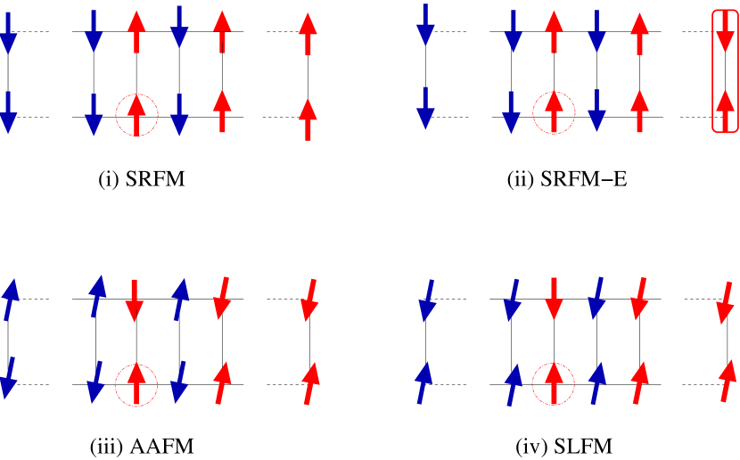
Figure 2: (Color online). Spin arrangements in (i) stripe rung ferromagnetic (SRFM), (ii) stripe rung ferromagnetic edge (SRFM-E), (iii) anisotropic antiferromagnetic (AAFM) and (iv) stripe leg ferromagnetic (SLFM) phases are shown. Arrows in the odd rungs (blue) and even rungs (red) represent $\sigma$-type and S type spins respectively. In subfigure (ii), the uncompensated dimer is shown in the box.

III.1 Quantum phase diagram

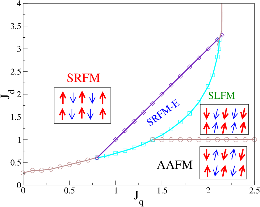
Figure 3: (Color online). Quantum phase diagram of the Ladder with open boundary condition is shown. Spin arrangements of the AAFM, the SLFM, the SRFM phases are shown inside the boxes.

In Fig. 3 the four phases, the SRFM, the SRFM-E, the AAFM and the SLFM are shown separated by five phase boundaries for $N=24$, and we notice that the phase boundaries weakly depend on the system size. These phase boundaries are determined based on energy crossovers and the correlation functions $C^{L}(r)$ and $C^{T}(r)$ by tuning $J_{d}$ and $J_{q}$. The large fraction of the phase space is covered by the SRFM phase and the AAFM phase has second largest contribution. It is interesting to note that the phase boundary of the AAFM and the SLFM is at $J_{d}/J=1$ for large $J_{q}$. Here, the bond order $<S_{i}.S_{i+1}>$ between the two $S$ spin along the rung form a perfect singlet dimer. The correlation length in $C^{L}(r)$ shrinks to one unit cell, but this phase is restricted to only this phase boundary. The strong singlet dimers along the rung at $B$ type sublattice ($\sigma-\sigma$) are formed on either sides of the phase boundary.

III.2 Ground state energy and excitation gap

The GS energy $E_{GS}$ of the system is doubly degenerate in major part of the parameter space, and $E_{GS}$ and the lowest excited state in $S^{z}_{tot}=0$ and 1 sectors are analyzed as shown in Fig. 4. The lowest state energy in $S^{z}_{tot}=0$ and 1 sectors are shown in Fig. 4.a for $J_{q}=0.2$. The lowest energy $E_{GS}$ in $S^{z}_{tot}=0$ sector initially increases with $J_{d}$ due to enhancement in the frustration induced by $J_{d}$ and it starts to decrease again for $J_{d}>0.33$, as the $J_{d}$ becomes dominant and frustration decreases and system goes to the SRFM phase. The peak of $E_{GS}$ indicates the phase boundary. For small $J_{q}$ the phase transition from the AAFM to the SRFM seems to be sharp as derivative of $E_{GS}$ is discontinuous as shown in Fig. 4 a. Whereas the change in $E_{GS}$ is continuous for large $J_{q}$ as shown in Fig. 4, therefore phase transition seems to be second order. In Fig. 4.b the lowest excited state in $S^{z}_{tot}=0$ and the lowest state in $S^{z}_{tot}=1$ sector are shown with black and red color line-symbols for $J_{q}=1$ respectively. Negative value of red curve indicates the $S^{z}_{tot}=1$ as GS and the state appears because of a singlet dimer pair formation between edge $S-S$ spins, if the chain starts with $\sigma-\sigma$ spin pair (odd rungs) and ends with $S-S$ spin pair (even rungs) as considered in the system. In this case, a pair of uncompensated ferromagnetically aligned $\sigma-\sigma$ pair gives rise to the $S^{z}_{tot}=1$ manifold. The boundaries for the SRFM-E is obtained by onset and end of the GS with $S^{z}_{tot}=1$ as shown in Fig. 4.b.

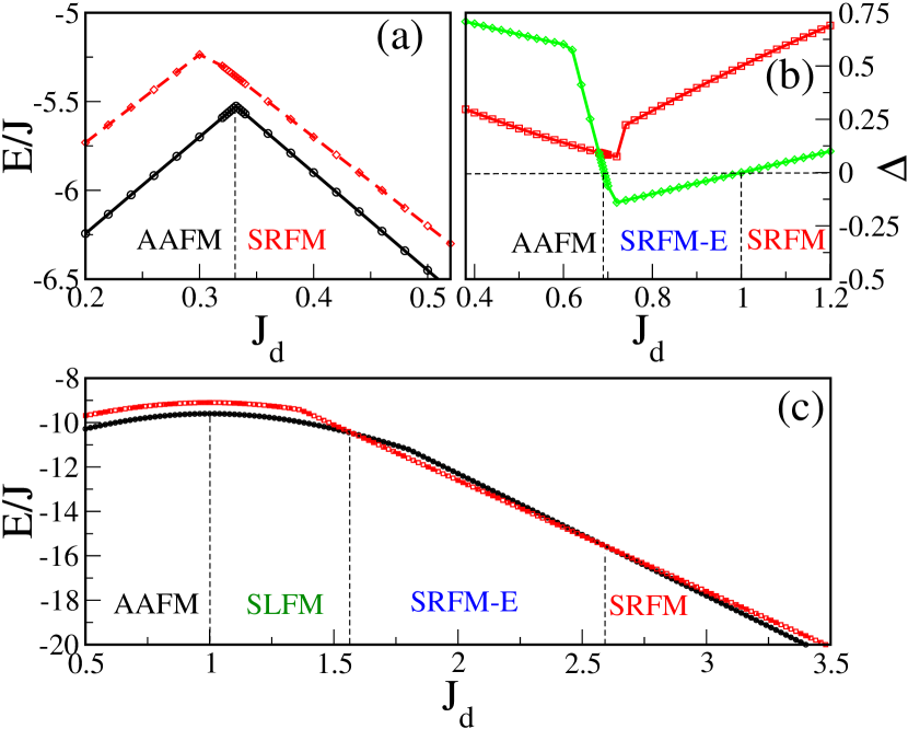
Figure 4: (Color online). (a) Black solid line and red dashed line represent energies ($E/J$) in two respective spin sectors: $S^{z}_{tot}=0$ and $S^{z}_{tot}=1$ for $J_{q}=0.2$, (b) $\Delta$ is the energy gap for $J_{q}=1.0$. Red solid line represents the lowest energy gap in $S^{z}_{tot}=0$ sector and green solid line represents the energy gap of the lowest state in $S^{z}_{tot}=1$ sector from the lowest state in $S^{z}_{tot}=0$ sector. (c) Black solid line and red dashed line represent energies ($E/J$) in two respective spin sectors: $S^{z}_{tot}=0$ and $S^{z}_{tot}=1$ for $J_{q}=1.8$. ($E/J$) and $\Delta$ in all the subfigures are shown for system size N=24.

In Fig. 4.c all four phases and their boundaries are shown for $J_{q}=1.8$. We notice that the maxima of doubly degenerate GS is the phase boundary between the AAFM and the SLFM phase, whereas, the onset and end of GS in the $S^{z}_{tot}=1$ is the phase boundary of the SRFM-E phase. In the SRFM phase, the GS is again in $S^{z}_{tot}=0$ sector. It is also evident from all three figures that $E_{GS}$ is continuous in large $J_{q}$ limit.

III.3 Correlation functions

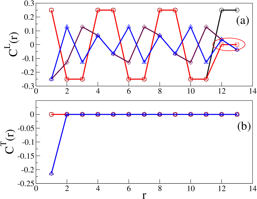
Figure 5: (Color online). (a) Longitudinal and (b) Transverse Correlation plots are shown. Black, red, maroon and blue colors in both of the subfigures, represent four respective phases; SRFM ($J_{q}=0.2$,$J_{d}=2.0$), SRFM-E ($J_{q}=1.6$,$J_{d}=1.25$), AAFM ($J_{q}=2.0$,$J_{d}=0.4$) and SLFM ($J_{q}=2.0$,$J_{d}=1.6$).

To understand the arrangement of spin in the GS, we study the two component: longitudinal $C^{L}(r)$ and transverse $C^{T}(r)$ correlations in four different phases as shown in Fig. 5. The reference site is at the lower leg of sublattice A ($S$-type spin) at mid of the ladder and the arrangement of distance r is shown in Fig. 1 . In the SRFM phase ($J_{q}=0.2,J_{d}=2.0$), the $C^{L}(r)$ shows long-range behavior and nearest neighbor along the rung is ferromagnetically aligned, whereas nearest neighbor along the leg is antiferromagnetically aligned. The $C^{T}(r)$ is zero for spins, therefore, GS is completely Ising like. In the SRFM-E ($J_{q}=1.6,J_{d}=1.25$), the correlation functions are same as that for the SRFM except at the boundary where the $C^{L}(r)$ goes to zero i.e the last pair of spins is decoupled from the ladder. The $C^{T}(r)$ is zero for all spins with respect to reference spin, but between edge rung spin pair $S-S$ it is -1/2. In the SLFM phase ($J_{q}=2.0,J_{d}=1.6$), the nearest rung spins are antiferromagnetically aligned, whereas along the leg nearest neighbor spins are ferromagnetically aligned. The nonzero value of $C^{T}(r)$ is restricted to nearest rung spin. However, in the limit $J_{q}=2.0,J_{d}=0.4$ (AAFM phase), the $C^{L}(r)$ is long-range and both the nearest spins along the rung and along the leg are antiferromagnetically aligned. The $C^{T}(r)$ is restricted to the only nearest rung spin and the value $C^{T}(r=1)$ increases with $J_{q}$ as shown in Fig. 5. It is also interesting to note that the long-range behavior in the correlation $C^{L}(r)$ melts with increasing $J_{q}$.
The AAFM phase is interesting due to highly anisotropy correlations in the system and also the rapid variation in the correlation with $J_{q}$. To our surprise, at $J_{d}=1$, two nearest spins along the rung ($S-S$ pairs) form perfect singlet dimers, and the GS of the system behaves like product of Ising and singlet dimers. To show the GS spin arrangement, $C^{L}(r)$ and $C^{T}(r)$ for $J_{d}=0.8,1$ and 1.2 for $J_{q}=2.0$ are plotted as a function of distance $r$ in Fig. 6. We notice finite value of $C^{L}(r)$ and $C^{T}(r)$ are restricted to nearest rung spin, whereas, $C^{L}(r)$ are non-collinear in nature in the neighborhood of $J_{d}=1$ for large $J_{q}$. For two values of $J_{d}=0.8$ and 1.2 for $J_{q}=2.0$, $C^{L}(r)$ shows non-collinear spin arrangement and the $C^{T}(r)$ is restricted to the same rung in A sublattice ($S$ spin) as shown in Fig. 6.

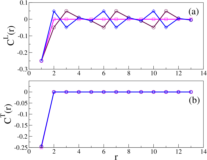
Figure 6: (Color online). (a) Longitudinal and (b) Transverse Correlations for three phases are shown. Maroon, magenta and blue colors in both of the subfigures are for AAFM ($J_{q}=2.0$, $J_{d}=0.8$), Perfect Dimer ($J_{q}=2.0$, $J_{d}=1.0$) and SLFM ($J_{q}=2.0$, $J_{d}=1.2$) phases respectively.

III.4 Exact thermodynamical properties

The spin model Hamiltonian in Eq. II have commuting bonds operators because Ising exchange interactions along the leg and diagonal of the ladder, therefore using transfer matrix method exact solution at finite temperature can be studied. In this paper, we study the low-temperature thermodynamical properties of our model using a suitably adapted transfer matrix method. Henceforth, our transfer matrix calculations assume periodic boundary condition (PBC) and we will be using the full Hamiltonian without the edge part ($\mathbf{H_{e}}=0$). The Hamiltonian for a single geometrical unit (Eq.II) can be reduced in the following manner:

$$\mathbf{H_{i}}=\frac{J_{q}}{2}\left(S_{2i,1}^{+}S_{2i,2}^{-}+S_{2i,2}^{+}S_{2i,1}^{-}\right)+J_{q}\left(S_{2i,1}^{z}S_{2i,2}^{z}\right)$$

$$+aS_{2i,1}^{z}+bS_{2i,2}^{z}+c+d.$$ (3)

Here a, b, c, d can be written in terms of the parameters $J_{c}$, $J_{cq}$, $J_{d}$ and $h$, and the spin operator $\sigma$ (see in appendix VI). In the equation $S^{+}$, $S^{-}$ are the creation and annihilation operators respectively for spin S.

Due to special construction of our model, we have $[\mathbf{H_{i}},\mathbf{H_{j}}]=0$ for any $i$ and $j$. This fact helps us to write the partition function of the total system as the trace of the $n$-th power of a small ($4\times 4$) transfer matrix (see the details in Appendix VI). The partition function for $N(=4n)$ number of spins, $Q_{N}(\beta)=Tr(e^{-\beta\textbf{H}})$ with $\beta$ being the inverse temperature can be written as,

$$Q_{N}(\beta)=\lambda_{1}^{n}+\lambda_{2}^{n}+\lambda_{3}^{n}+\lambda_{4}^{n},$$

where four $\lambda$’s are the eigenvalues of the transfer matrix. If $\lambda_{1}$ is the largest eigenvalue then for large $N$, $Q_{N}(\beta)={\lambda_{1}}^{n}$ (see in appendix VI). Using the partition function $Q_{4}(\beta)$ ($=\lambda_{1}$, partition function for a geometric unit), the thermodynamic quantities can be calculated using the following standard formulas: free energy (per geometrical unit) $F(T)=-k_{B}T\log{Q_{4}(\beta)}$, average energy $E(T)=k_{B}T^{2}\frac{d}{dT}\log{Q_{4}(\beta)}$, specific heat $C_{v}(T)=\left(\frac{\partial E(T)}{\partial T}\right)_{v}$, magnetization $M(T)=-\frac{\partial F(T)}{\partial h}$, magnetic susceptibility $\chi(T)=\frac{\partial M(T)}{\partial h}$, and entropy $S(T)=-\left(\frac{\partial F(T)}{\partial T}\right)$.

In $T\rightarrow 0$ limit, the largest eigenvalue $\lambda_{1}$ can be written as $\lambda_{1}=e^{\frac{\beta(1+J_{q}(1+2\Delta_{2}))}{4}}+e^{\frac{\beta(4J_{d}-J_{q}+3))}{4}}$, where $\Delta_{2}=\sqrt{1+4\frac{(1-J_{d})^{2}}{J_{q}^{2}}}$ (see in appendix VI). In the zero-temperature limit, the first exponential term in the expression of $\lambda_{1}$ dominates over the second exponential term in the regimes corresponding to the AAFM and the SLFM phases, while in the regime corresponding to the SRFM phase, the opposite happens. In this $T\rightarrow 0$ limit, the free energy takes the following forms in the regimes corresponding to the SRFM and the AAFM phases respectively: $F_{SRFM}=-\frac{4J_{d}-J_{q}+3}{4}$ and $F_{AAFM}=F_{SLFM}=-\frac{1+J_{q}(1+2\Delta_{2})}{4}$. In this zero temperature limit, in all the three regimes, the entropy and the specific heat are found to be zero. These results match well with our numerical calculations using the full expression of $\lambda_{1}$ (see in appendix VI).

To understand the thermodynamic behavior at the non-zero temperatures, we calculate four thermodynamical quantities $E(T)$, $C_{v}(T)$, $S(T)$ and $\chi(T)$ for three parameter regimes and are shown in Fig. 7. We use full expression of the largest eigenvalue $\lambda_{1}$ for this numerical calculation. It may be noted that the different ground state phases of the system, which were obtained with open boundary condition for the finite system sizes, may not have direct consequences in our low-temperature thermodynamic results as the thermodynamic calculations are done with periodic boundary condition for thermodynamically large system. Here, our main purpose of studying the thermodynamical quantities is to see how these quantities change across the parameter regimes of interest.

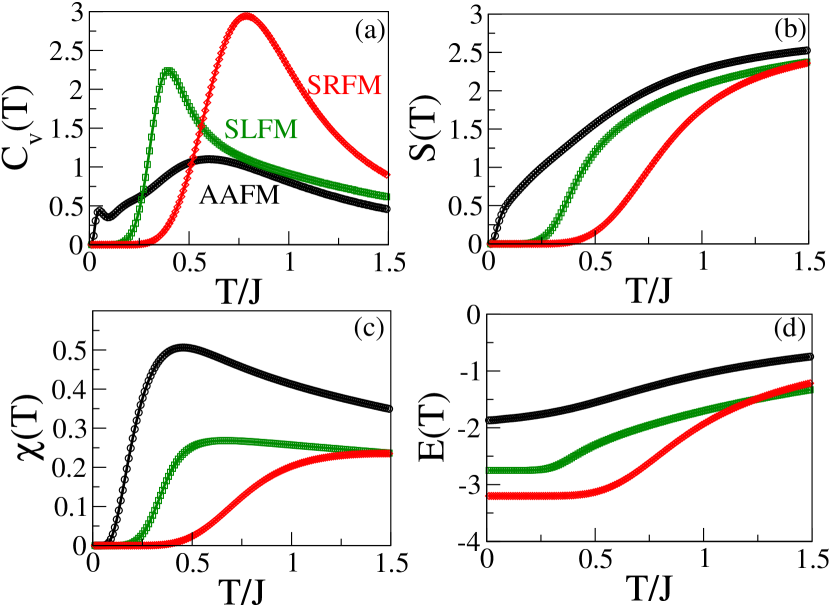
Figure 7: (Color online). (a) Specific heat ($C_{v}(T)$), (b) Entropy ($S(T)$), (c) Magnetic susceptibility ($\chi(T)$) and (d) Average Energy ($E(T)$) plots are shown. Black, red and green curves in each of the subfigures, represent three phases: AAFM ($J_{q}=2.0$, $J_{d}=0.5$), SLFM ($J_{q}=2.0$, $J_{d}=2.5$) and SRFM ($J_{q}=0.2$, $J_{d}=2.5$) respectively.

The $C_{v}(T)$ of the three different phases show different features as shown in Fig. 7.a. In the AAFM region where $J_{d}$ is weak and $J_{q}$ is dominant, $C_{v}(T)$ shows a small peak near the $T\rightarrow 0$, which may be because of small gap due to small excitation gap in $S^{z}_{tot}=0$ sector, and then there is broad maxima at higher temperature, which is similar to the Heisenberg spin dimer system. The weak singlet dimer is formed along the rung of $S-S$ spins and that may give a broad peak at moderate temperature. The $C_{v}(T)$ in the SLFM phase shows very sharp peak and long tail, but have vanishing small value for $T/J<0.09$ due to finite energy gap in the system. In the SRFM phase, this quantity is vanishingly small for $T/J<0.35$ due to large magnetic gap which makes the system to thermalise at higher temperature and a relatively higher peak at $T/J=0.75$. The entropy $S(T)$ is in some sense is the measure of thermalisation, which in three different phases of the system are shown in Fig. 7.b. In the AAFM phase, there is a small non-magnetic gap. Whereas, in other two phases $S(T)$ is vanishingly small for $T/J<0.1$ due to large energy gap and thereafter it increases monotonically.

The magnetic susceptibility $\chi(T)$ in these three phases are shown in Fig. 7.c and all the $\chi(T)$ have small values in all three phases for $T/J<0.1$. It has a broad maxima and small gap in the AAFM phase due to the formation of singlet dimer, and for breaking the weak singlet dimer it costs finite energy, therefore, singlet-triplet gap is finite. The $\chi(T)$ in the SRFM phase has dominant Ising interaction, therefore, there is a finite energy gap and sharp peak similar to the 1D Ising system. In the SLFM phase there is large magnetic gap as it requires breaking of strong rung interaction, and this leads to small $\chi(T)$ at low temperature and exponential increase in the $\chi(T)$. The average internal energy $E(T)$ shows a linear variation with $T$ in the AAFM phase, but almost constant value of $E(T)$ for $T<0.09$ indicates the gap in the SLFM phase as shown in Fig. 7.d. In the SRFM phase, variation of the energy is almost constant for $T/J<0.35$ due to large energy gap and it varies linearly with $T$ thereafter.

IV Summary and conclusion

In this paper, we consider a very general anisotropic Heisenberg-Ising model on ladder geometry with alternate Heisenberg and Ising exchange rung interactions, whereas the exchange interactions along the leg and along the diagonal of the ladder are Ising type. We construct a quantum phase diagram of the model Hamiltonian in Sec.II, and have shown that there are four quantum phases: (i) the AAFM, (ii) the SRFM, (iii) the SRFM-E and (iv) the SLFM which appear due to competing interactions and anisotropy in the system. The GS is doubly degenerate and have finite magnetic gap in most of the parameter space and to our surprise, exact dimer state along the rung in A sublattice (rungs with isotropic exchange interactions) appears for $J_{d}=1$ and large $J_{q}$ limit. However, weak dimer appears along rung of spin $S$ near to $J_{d}=1$.

The thermal properties of this system are also studied analytically using the transfer matrix method. Four temperature dependent properties like specific heat $C_{v}(T)$, average internal energy $E(T)$, entropy $S(T)$ and magnetic susceptibility $\chi(T)$ are studied in three different phases: the SRFM, the SLFM and the AAFM. In large $\frac{J_{q}}{J_{d}}$ regime (AAFM phase), $C_{v}$ shows a small peak at small $T$ due to a small excitation gap, whereas it has vanishingly small $\chi$ upto $T<0.09$ due to finite magnetic gap in the SLFM phase. Due to large excitation gap in the SRFM phase, all four quantities vanish for $T<0.35$.

In conclusion, we have studied a highly anisotropic model on a ladder geometry and the model Hamiltonian exhibits four interesting GS phases. The thermodynamic quantities like $Cv(T)$, $\chi(T)$, $E(T)$ and $S(T)$ are also studied using the transfer matrix method. This model may be realized in Cu or Vi based materials having magnetic interaction confined in ladder like geometry and the material should also have large anisotropy to ensure the Ising exchange.

V Acknowledgements

MK thanks DST India for a Ramanujan Fellowship SR/S2/RJN-69/2012. MK thanks SMST Department of IIT (BHU) for the hospitality during his visit. SS thanks SNBNCBS for supporting him under EVLP during his stay at the Centre when this work was started.

VI Appendix

The partition function for $N$ sites, $Q_{N}(\beta)$ with Hamiltonian $H$ can be written as-

$$Q_{N}(\beta)=Tr\left(e^{-\beta\textbf{H}}\right)$$ (4)

where, Tr means trace of the matrix, $\beta=1/\left(k_{B}T\right)$ and $k_{B}$ is the Boltzmann constant. Using explicit configuration basis for the system, Eq. 4 is rewritten in the following form,

$$Q_{N}(\beta)=\sum_{\{\sigma,S\}}<\cdots,\sigma_{2i-1,1},\sigma_{2i-1,2},S_{2i,1},S_{2i,2},\cdots\mid e^{-\beta\mathbf{H}}\mid\cdots,\sigma_{2i-1,1},\sigma_{2i-1,2},S_{2i,1},S_{2i,2},\cdots>,$$

here the summation is over all possible configurations $\{\sigma,S\}$ of the system. For a given configuration, $|\cdots,\sigma_{2i-1,1},\sigma_{2i-1,2},S_{2i,1},S_{2i,2},\cdots>$ represents a basis state. Since for our system, the Hamiltonians corresponding to different units commute with each other, we further get,

$$Q_{N}(\beta)=\sum_{\sigma}<\cdots,\sigma_{2i-1,1},\sigma_{2i-1,2},\cdots\mid\prod_{i=1}^{n}\mathbf{T}_{i}\mid\cdots,\sigma_{2i-1,1},\sigma_{2i-1,2},\cdots>$$

where $T_{i}=\sum_{\{S\}_{i}}<S_{2i,1},S_{2i,2}\mid e^{-\beta\mathbf{H_{i}}(\sigma,S)}\mid S_{2i,1},S_{2i,2}>$. Here the summation is over $\{S\}_{i}$ which represents all possible configurations of spins $S_{2i,1}$ and $S_{2i,2}$ (from the $i^{th}$ unit). It may be noted that $T_{i}$ does not contain the components of spin $S$ operators and it has only $\sigma$ variables, namely, $\sigma_{2i-1,1},\sigma_{2i-1,2},\sigma_{2i+1,1}$ and $\sigma_{2i+1,2}$. This form is well-known with $\mathbf{T}_{i}$ being the transfer operator. Introducing identity operators $I=\sum_{\{\sigma\}_{i}}|\sigma_{2i-1,1},\sigma_{2i-1,2}><\sigma_{2i-1,1},\sigma_{2i-1,2}|$ between successive $\mathbf{T}$ operators, we can finally write the partition function as the trace of the $n$-th power of a small ($4\times 4$) transfer matrix $\mathbf{P}$. We have,

$$Q_{N}(\beta)=Tr(\mathbf{P}^{n}),$$

where $n$ is the number of geometrical units. The elements of the transfer matrix are given by

$$P_{(\sigma_{2i-1,1},\sigma_{2i-1,2}),(\sigma_{2i+1,1},\sigma_{2i+1,2})}=<\sigma_{2i-1,1},\sigma_{2i-1,2}\mid\mathbf{T}_{i}\mid\sigma_{2i+1,1},\sigma_{2i+1,2}>$$ (5)

Before we construct and diagonalise the $\mathbf{P}$ matrix, we first need to carry out the trace over the configurations $\{S\}_{i}$ to find out the form of $\mathbf{T}_{i}$. Since $\mathbf{T}_{i}=\sum_{\{S\}_{i}}<S_{2i,1},S_{2i,2}\mid e^{-\beta\mathbf{H_{i}}(\sigma,S)}\mid S_{2i,1},S_{2i,2}>$, if we take the eigenstate basis of $\mathbf{H}_{i}$, we will get $\mathbf{T}_{i}$ as the summation over exponential of eigenvalues of $-\beta\mathbf{H}_{i}$. Next we calculate eigenvalues of $\mathbf{H}_{i}$ operator.

By considering,
$a=J_{d}\left(\sigma_{2i-1,2}^{z}+\sigma_{2i+1,2}^{z}\right)+J_{cq}\left(\sigma_{2i-1,1}^{z}+\sigma_{2i+1,1}^{z}\right)+h$
$b=J_{d}\left(\sigma_{2i-1,1}^{z}+\sigma_{2i+1,1}^{z}\right)+J_{cq}\left(\sigma_{2i-1,1}^{z}+\sigma_{2i+1,1}^{z}\right)+h$
$c=\frac{J_{c}}{2}\left(\sigma_{2i-1,1}^{z}\sigma_{2i-1,1}^{z}+\sigma_{2i+1,1}^{z}\sigma_{2i+1,2}^{z}\right)$
$d=\frac{h}{2}\left(\sigma_{2i-1,1}^{z}+\sigma_{2i-1,2}^{z}+\sigma_{2i+1,1}^{z}+\sigma_{2i+1,2}^{z}\right)$,
Hamiltonian (Eq. III.4 ) for the $i^{th}$ geometrical unit can be written as-

$$\mathbf{H_{i}}=\frac{J_{q}}{2}\left(S_{2i,1}^{+}S_{2i,2}^{-}+S_{2i,1}^{-}S_{2i,2}^{+}\right)+J_{q}\left(S_{2i,1}^{z}S_{2i,2}^{z}\right)+aS_{2i,1}^{z}+bS_{2i,2}^{z}+c+d$$

By taking $f=c+d$, we can write down the following Hamiltonian matrix in the eigenstate basis of $S_{2i,1}^{z}S_{2i,2}^{z}$ operator,

$${H_{i}}=\begin{pmatrix}\frac{J_{q}}{4}+\frac{(a+b)}{2}+f&0&0&0\\ 0&\frac{-J_{q}}{4}+\frac{(a-b)}{2}+f&\frac{J_{q}}{2}&0\\ 0&\frac{J_{q}}{2}&\frac{-J_{q}}{4}-\frac{(a-b)}{2}+f&0\\ 0&0&0&\frac{J_{q}}{4}-\frac{(a+b)}{2}+f\\ \end{pmatrix}.$$

The Hamiltonian matrix comes up with its four eigenvalues from three $S^{z}_{SS}$ sectors based on S-S pairs-
(i) From $S^{z}_{SS}=1$ sector (formed by S-S pair)
$\theta_{1}=(f+\frac{J_{q}}{4})+\frac{(a+b)}{2}$
(ii) From $S^{z}_{SS}=-1$ sector (formed by S-S pair)
$\theta_{2}=(f+\frac{J_{q}}{4})-\frac{(a+b)}{2}$
(iii) From $S^{z}_{SS}=0$ sector (formed by S-S pair)
$\theta_{3}=(f-\frac{J_{q}}{4})+\frac{\sqrt{J_{q}^{2}+(a-b)^{2}}}{2}$
$\theta_{4}=(f-\frac{J_{q}}{4})-\frac{\sqrt{J_{q}^{2}+(a-b)^{2}}}{2}$.

We note that the eigenvalues ($\theta_{k}$) are functions of $\sigma$ variables, namely $\sigma_{2i-1,1},\sigma_{2i-1,2},\sigma_{2i+1,1}$ and $\sigma_{2i+1,2}$. Using these eigenvalues, we rewrite $\mathbf{T}_{i}$ as,

$$\mathbf{T}_{i}=\sum_{\{S\}_{i}}<S_{2i,1},S_{2i,2}\mid e^{-\beta\mathbf{H_{i}}(\sigma,S)}\mid S_{2i,1},S_{2i,2}>$$

$$~{}~{}~{}=\sum_{k=1}^{4}e^{-\beta\theta_{k}}.$$

Without magnetic field (h=0), the Transfer Matrix ($\mathbf{P}$) takes the following form (using Eq. 5)-

$$\mathbf{P}=\begin{pmatrix}p&q&q&r\\ q&s&u&q\\ q&u&s&q\\ r&q&q&p\\ \end{pmatrix},$$

here,

$$p=2e^{\frac{-\beta}{4}}[Q^{-1}Cosh{\beta(1+J_{d})}+QCosh(\frac{\beta J_{q}}{2})]$$

$$q=2[Q^{-1}Cosh{\beta((1+J_{d})/2)}+QCosh(\frac{\beta J_{q}\Delta_{1}}{2})]$$

$$r=2e^{\frac{-\beta}{4}}[Q^{-1}+QCosh(\frac{\beta J_{q}}{2})]$$

$$s=2e^{\frac{\beta}{4}}[Q^{-1}+QCosh(\frac{\beta J_{q}\Delta_{2}}{2})]$$

$$u=2e^{\frac{\beta}{4}}[Q^{-1}+QCosh(\frac{\beta J_{q}}{2})]$$

$$\Delta_{1}=\sqrt{1+\frac{(1-J_{d})^{2}}{J_{q}^{2}}}$$

$$\Delta_{2}=\sqrt{1+4\frac{(1-J_{d})^{2}}{J_{q}^{2}}}$$

$$Q=e^{\frac{\beta J_{q}}{4}}.$$

The above Transfer Matrix has $4$ simple eigenvalues $\lambda_{1}$, $\lambda_{2}$, $\lambda_{3}$, $\lambda_{4}$ as follows

$$\mathbf{\lambda_{1}}=\frac{(p+r+s+u)}{2}$$

$$+\frac{\sqrt{(p+r+s+u)^{2}+16q^{2}-4(p+r)(s+u)}}{2}$$

$$\mathbf{\lambda_{2}}=\frac{(p+r+s+u)}{2}$$

$$-\frac{\sqrt{(p+r+s+u)^{2}+16q^{2}-4(p+r)(s+u)}}{2}$$

$$\mathbf{\lambda_{3}}=(p-r)$$

$$\mathbf{\lambda_{4}}=(s-u).$$

It is to be noted that $\lambda_{1}$ is the largest eigenvalue here.

In the special case with $T\rightarrow 0$ limit, the largest eigenvalue can be approximated as- $\lambda_{max}=(p+r+s+u)$.
Explicitly, we have,

$$\mathbf{\lambda_{max}}=$$

$$(2e^{\frac{\beta(3J_{q}-1)}{4}}+e^{\frac{\beta(4J_{d}+3-J_{q})}{4}}+5e^{\frac{\beta(1-J_{q})}{4}}+e^{\frac{\beta(1+J_{q}(1+2\Delta_{2})}{4}}).$$

References

- (1) S. E. Dutton, M. Kumar, M. Mourigal, Z. G. Soos, J. J. Wen, C. L. Broholm, N. H. Andersen, Q. Huang, M. Zbiri, R. Toft-Petersen, R. J. Cava, Phys. Rev. Lett. , 187206 (2012).
- (2) A. W. Sandvik, E. Dagotto, and D. J. Scalapino, Phys. Rev. B , R2934 (1996).
- (3) E. Dagotto and T. M. Rice, Science , 618 (1996).
- (4) N. Maeshima, M. Hagiwara, Y. Narumi, K. Kindo, T. C. Kobayashi, and K. Okunishi, J. Phys.: Cond. Matt. , 3607 (2003).
- (5) D. C. Johnston, J. W. Johnson, D. P. Goshorn, and A. J. Jacobson, Phys. Rev. B , 219 (1987).
- (6) M. T. Hutchings, J. M. Milne, and H Ikeda, Journal of Physics C: Solid State Physics , L739 (1979).
- (7) C.L. Z. S. Park Y. J. Choi, and S. W. Cheon, Phys. Rev. Lett. , 057601 (2007).
- (8) Mourigal, M, Enderle, M, Fåk, B. and Kremer, R. K. and Law, J. M. and Schneidewind, A. and Hiess, A. and Prokofiev, A., Phys. Rev. Lett. , 027203 (2012).
- (9) S. L. Drechsler, O. Volkova, A. N. Vasiliev, N. Tristan, J. Richter, M. Schmitt, H. Rosner, J. Málek, R. Klingeler, A. A. Zvyagin, and B. Büchner, Phys. Rev. Lett. , 077202 (2007).
- (10) S. E. Dutton, M Kumar, Z. G. Soos, C. L. Broholm, and R. J. Cava, J. Phys.: Cond. Matt. , 166001 (2012).
- (11) M. Kumar, A. Parvej, and Z. G. Soos, J. Phys.: Cond. Matt. , 316001 (2015).
- (12) K. Okamoto and K. Nomura, Phys. Lett. A , 433 (1992).
- (13) R. Chitra, S. Pati, H. R. Krishnamurthy, D. Sen, and S. Ramasesha, Phys. Rev. B , 6581 (1995).
- (14) Z.G.Soos, A.Parvej and M.Kumar, J. Phys.: Condens. Matter , 175603(2016).
- (15) C. K. Majumdar and D. K. Ghosh, J. Math. Phys. , 1388(1969).
- (16) S. R. White, R. M. Noack and D. J. Scalapino, Phys. Rev. Lett. , 886(1994).
- (17) S. R. White and I. Affleck, Phys. Rev. B , 9862 (1996).
- (18) B. S. Shastry and B. Sutherland, Phys. Rev. Lett. , 964(1981).
- (19) F. D. M. Haldane, Phys. Rev. B , 4925 (1982).
- (20) A. V. Chubukov, Phys. Rev. B , 4693 (1991).
- (21) S. Furukawa, M. Sato, S. Onoda, and A. Furusaki, Phys. Rev. B , 094417 (2012).
- (22) M. E. Zhitomirsky and H. Tsunetsugu, Europhys. Lett. , 37001 (2010).
- (23) A. Parvej and M. Kumar, Phys. Rev. B , 054413 (2017).
- (24) I. U. Heilmann, G. Shirane, Y. Endoh, R. J. Birgeneau, and S. L. Holt, Phys. Rev. B , 3530 (1978).
- (25) I. Umegaki, H. Tanaka, N. Kurita, T. Ono, M. Laver, C. Niedermayer, C. Rüegg, S. Ohira-Kawamura, K. Nakajima, and K. Kakurai, Phys. Rev. B , 174412 (2015).
- (26) D. C. Johnston, Phys. Rev. B , 13009 (1996).
- (27) T. Barnes, E. Dagotto, J. Riera, and E. S. Swanson, Phys. Rev. B , 3196 (1993).
- (28) E. Manousakis, Rev. Mod. Phys. , 1 (1991).
- (29) Y. Singh and P. Gegenwart, Phys. Rev. B , 064412 (2010).
- (30) M. Mourigal, M. Enderle, R. K. Kremer, J. M. Law, and B. Fåk, Phys. Rev. B , 100409 (2011).
- (31) M. Enderle, B. Fåk, H. J. Mikeska, R. K. Kremer, A. Prokofiev, and W. Assmus, Phys. Rev. Lett. , 237207 (2010).
- (32) Z. Seidov, T. P. Gavrilova, R. M. Eremina, L. E. Svistov, A. A. Bush, A. Loidl and H. A. Krug von Nidda, Phys. Rev. B , 224411 (2017).
- (33) M Kumar, S. E. Dutton, R. J. Cava, and Z. G. Soos, J. Phys.: Cond. Matt. , 136004 (2013).
- (34) M. Kumar, A.Parvej, and Z. G Soos, J. Phys.: Cond. Matt. , 175603 (2016).
- (35) J. Sirker, Phys. Rev. B , 014419 (2010).
- (36) T. Hamada, J. Kane, S. Nakagawa, and Y. Natusume,J. Phys. Soc. Jpn. , 1891 (1988).
- (37) P. Anderson, Materials Research Bulletin , 153 (1973).
- (38) P. Fazekas and P. W. Anderson, The Philosophical Magazine: A Journal of Theoretical Experimental and Applied Physics , 423 (1974).
- (39) C. K. Majumdar and D. K. Ghosh, J. Math. Phys. , 1399 (1969).
- (40) Sebastian Eggert. Phys. Rev. B , R9612 (1996).
- (41) M. Kumar, S. Ramasesha, and Z. G. Soos, Phys. Rev. B ,054413 (2010).
- (42) T. Tonegawa and I. Harada, J. Phys. Soc. Jpn. , 2153 (1987).
- (43) M. A. Korotin, I. S. Elfimov, V. I. Anisimov, M. Troyer, and D. I. Khomskii, Phys. Rev. Lett. , 1387 (1999).
- (44) M. A. Korotin, V. I. Anisimov, T Saha-Dasgupta, and I Dasgupta, Journal of Physics: Cond. Matt. , 113 (2000).
- (45) Lucile Savary and Leon Balents, Rep. Prog. Phys. , 016502 (2017).
- (46) D. Maiti, M. Kumar, Phys. Rev. B , 24511 (2019).
- (47) Curély. J, Georges. R, Drillon. M, Phys. Rev. B , 6243 (1986).
- (48) Strečka. J, Michal Jaˇsˇcur. M, J. Phys.: Cond. Matt. , 4519 (2003).
- (49) H. Rezania, Journal of Magnetism and Magnetic Materials , 68 (2015).
- (50) E. Čižmár, E. and Ozerov, M and Wosnitza, J. and Thielemann, B. and Krämer, K. W. and Rüegg, Ch. and Piovesana, O. and Klanjšek, M. and Horvatić, M. and Berthier, C and Zvyagin, S. A, Phys. Rev. B , 054431 (2010).
- (51) Thielemann, B. and Rüegg, Ch. and Ronnow, H. M. and Läuchli, A. M. and Caux, J. S. and Normand, B. and Biner, D. and Krämer, K. W. and Güdel, H.-U. and Stahn, J. and Habicht, K. and Kiefer, K. and Boehm, M. and McMorrow, D. F. and Mesot, J, Phys. Rev. Lett. , 107204 (2009).
- (52) Onofre Rojas and J. Strečka and S.M. de Souza, Solid State Communications , 68 (2016).
- (53) T. Verkholyak, J. Strečka, Cond. Matt. Phys. , 13601 (2013).
- (54) T. Verkholyak and J. Streka, J. Phys. A: Math. Theor. , 305001 (2012).
- (55) Karl’ová, Katarína and Strečka, Jozef and Lyra, Marcelo L, Phys. Rev. E. , 042127 (2019).
- (56) S. Sahoo, J. P. Sutter, and S. Ramasesha, Journal of Statistical Physics , 181193 (2012).
- (57) Davidson, Ernest R., Journal of Computational Physics, , 87 (1975).
- (58) Kerson Huang, ISBN-13 : 978-8126518494