Moiré Commensurability and the Quantum Anomalous Hall Effect
in Twisted Bilayer Graphene on Hexagonal Boron Nitride

Abstract

The quantum anomalous Hall (QAH) effect is sometimes observed in twisted bilayer graphene (tBG) when it is nearly aligned with an encapsulating hexagonal boron nitride (hBN) layer. We propose that the appearance or absence of the QAH effect in individual devices could be related to commensurability between the graphene/graphene and graphene/hBN moiré patterns. We identify a series of points in the $\displaystyle(\theta_{{\rm GG}},\theta_{{\rm GBN}})$ twist-angle space at which the two moiré patterns are commensurate, allowing moiré band theory to be applied, and show that the band Chern numbers are in this case sensitive to a rigid in-plane hBN displacement. Given this property, we argue that the QAH effect is likely only when i) the $\displaystyle(\theta_{{\rm GG}},\theta_{{\rm GBN}})$ twist-angle-pair is close enough to a commensurate point that the two moiré patterns yield a supermoiré pattern with a sufficiently long length scale, and ii) the supermoiré has a percolating topologically non-trivial QAH phase. For twist angles far from commensurability, the hBN layer acts as a source of disorder that can destroy the QAH effect. Our proposal can explain a number of current experimental observations. Further experimental studies that can test this proposal more directly are suggested.

I Introduction

Two graphene sheets that have a small orientational misalignment (twisted bilayer graphene - tBG) form a quasiperiodic moiré superlattice, whose electronic structure is well-described by moiré band theory. Bistritzer and MacDonald (2011) Correlated insulating states, Cao et al. (2018a) Chern insulators, Sharpe et al. (2019); Serlin et al. (2020); Nuckolls et al. (2020); Saito et al. (2020a) and superconductivity Cao et al. (2018b); Lu et al. (2019); Yankowitz et al. (2019); Saito et al. (2020b) have been observed in tBG when the twist angle is close to a magic angle that enables strong correlation physics associated with exceptionally flat moiré bands. The introduction of twist angle as a new tunable degree of freedom has now been exploited to create strong correlations in a variety of different multi-layer van der Waals systems. Chen et al. (2019); Shen et al. (2020); Cao et al. (2020); Spanton et al. (2018); Wang et al. (2020); Regan et al. (2020); Liu et al. (2020)

Recent experiments have shown both non-quantized Sharpe et al. (2019) and quantized Serlin et al. (2020); Tschirhart et al. (2020) anomalous Hall effects can occur in magic angle twisted bilayer graphene when at least one graphene layer is nearly aligned with an encapsulating hexagonal boron nitride (hBN) layer, and the number of carriers per moiré period is close to an odd integer. The anomalous Hall effect is normally understood in terms of a mean-field picture, in which it arises from a combination of spontaneous valley polarization and non-zero Chern numbers of the valley-projected flat moiré bands induced by violation of inversion symmetry ($\displaystyle\mathcal{C}_{2}$).Xie and MacDonald (2020); Po et al. (2018); Zhang et al. (2019a, b); Bultinck et al. (2020) Somewhat mysteriously, the anomalous Hall effect is not always present even with hBN alignment.

The theoretical description of hBN encapsulated tBG runs into a fundamental difficulty when one or both hBN layers are nearly aligned with the tBG layers. Because of the small lattice constant mismatch between graphene and hBN, the nearly-aligned hBN layers produce additional moiré patterns Moon and Koshino (2014); Wallbank et al. (2015); Jung et al. (2014, 2015, 2017); Lin and Ni (2019) which are not in general commensurate with the moiré pattern of tBG. Therefore, the low-energy Hamiltonian is only quasi-periodic, disallowing all the simplifications that come from Bloch’s theorem. Similar moiré pattern interplays can also arise in twisted trilayer graphene.Zhu et al. (2020a) Most of the existing theoretical work on the anomalous Hall effect Zhang et al. (2019b); Bultinck et al. (2020) and related properties Wu and Das Sarma (2020); Repellin et al. (2020); Zhu et al. (2020b); Alavirad and Sau (2019); Chatterjee et al. (2020); Zhang et al. (2020) of tBG/hBN and hBN/tBG/hBN systems employs a highly simplified model in which only the spatially average sublattice energy difference is retained in the graphene/hBN moiré potentials. The justification for this expediency is not obvious, since the spatially averaged and position-dependent tBG/hBN interaction terms have similar energy scales Jung et al. (2017) and are therefore at first sight equally important.

The aim of this paper is to study the effect of the interplay between the moiré patterns on the anomalous Hall effect of encapsulated tBG. For definiteness we will assume that only one of the encapsulating hBN layers is aligned, which allows us to restrict our attention to tBG/hBN trilayers. In mean-field theory spontaneous valley polarization occurs when the moiré bands are sufficiently narrow to satisfy a Stoner criterion. It follows that both criteria for a quantized anomalous Hall effect, topologically non-trivial valley-projected bands and valley polarization, are simply related to the electronic structure issues on which we focus.

We notice that at particular combinations of the two twist angles, $\displaystyle\theta_{{\rm GG}}$ between the two graphene layers and $\displaystyle\theta_{{\rm GBN}}$ between the hBN and its adjacent graphene layer, the two moiré patterns are commensurate. The system is then periodic in a larger unit cell, allowing the use of Bloch’s theorem with both moiré patterns present. Recent papers Cea et al. (2020); Lin and Ni (2020) have noticed several such commensurate points in the twist angle space and we provide a general description of all commensurate geometries. For a commensurate system, rigid translation of the hBN layer by $\displaystyle\boldsymbol{d}$ at fixed twist angle changes the moiré band structures, and even moiré band Chern numbers.Cea et al. (2020) We characterize this dependence in terms of maps of Chern numbers and bandwidths vs. $\displaystyle\boldsymbol{d}$, from which electronic properties can be estimated.

A supermoiré pattern, also known as a moiré of moiré, is formed when the two moiré patterns are nearly, but not exactly commensurate. Supermoiré electronic structure has been studied in hBN/graphene/hBN trilayers Wang et al. (2019a); Leconte and Jung (2019); Andelkovic et al. (2020) and in twisted trilayer graphene, Zhu et al. (2020c, a); Tsai et al. (2019) but not yet in tBG/hBN. We point out here that the supermoiré can be viewed as a commensurate structure with spatially varying $\displaystyle\boldsymbol{d}$. Thus its electronic properties can be well described by a local moiré band picture, where local properties are defined by the local Hamiltonian $\displaystyle H(\boldsymbol{r})=H(\boldsymbol{d}(\boldsymbol{r}))$, with $\displaystyle H(\boldsymbol{d})$ the Hamiltonian of the commensurate structure. In this picture, the Chern number vs. $\displaystyle\boldsymbol{d}$ map expands to a spatial Chern number phase pattern, which is reminiscent of the percolationTrugman (1983) picture and of the Chalker-Coddington model Chalker and Coddington (1988); Marston and Tsai (1999) of the quantum Hall effect. In the present case, however, there are also semimetal phases due to overlaps between the valence and conduction bands that are indirect in momentum space. For the quantum anomalous Hall (QAH) effect the possible presence of regions in which the Stoner criterion for spontaneous valley polarization is not satisfied because of locally larger bandwidths is also relevant.

In this local picture a global QAH effect can appear only if the following two conditions are satisfied: i) the supermoiré period must be long enough that edge states between topologically distinct phases do not couple to each other and ii) a topologically nontrivial insulating phase must percolate across the device. The first condition is always satisfied over a finite range of twist angles close to a commensurate point and the second condition can usually be satisfied by varying the electrical potential difference $\displaystyle U$ between layers by applying a gate-controlled out-of-plane electric field.

In the opposite limit in which the two moiré patterns are far from being commensurate and the local moiré band picture fails, we assume that the moiré periodic part of the hBN potential acts like a disorder potential. The moiré bands of tBG are then widened by scattering from the hBN potential. In some cases this broadening effect may also make the full bandwidth exceed the interaction strength, standing in the way of spontaneous valley polarization and therefore of the anomalous Hall effect. Our proposals provide a possible explanation for a number of experimental observations, but are not conclusively established by exisiting experiments.

This paper is organized as follows: In Sec. II we first identify the commensurate twist angle pairs, and then discuss the geometry of tBG/hBN supermoiré systems in terms of proximity to these commensurate points. In Sec. III.1 we describe the continuum model we use to investigate the electronic structure. In Sec. III.2 we present our results for the spatial pattern of tBG/hBN supermoiré’s phases calculated from our model in a local-band approximation. In Sec. III.3 we estimate the twist angle windows within which QAH effects can occur in tBG/hBN supermoiré. In Sec. III.4 we analyze the limit in which the two moiré patterns are far from being commensurate. Then in Sec. IV, we use our results to provide possible explanations of current experiments and suggest further experimental approaches to test our proposals in the future. Sec. V contains the summary and main conclusions of this paper.

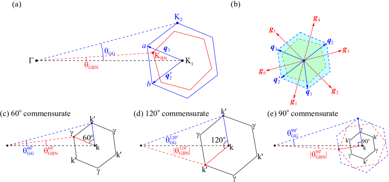
Figure 1: Schematic reciprocal space geometry of a tBG/hBN system: (a)-(b) Generic twist angles: $\displaystyle K_{1}$, $\displaystyle K_{2}$ and $\displaystyle K_{\rm BN}$ are Brillouin-zone corner points of graphene layer 1, graphene layer 2, and hBN, respectively. The mBZs of the G1/G2 and G1/hBN moiré patterns are illustrated by blue and red hexagons respectively; (c) $\displaystyle 60^{\circ}$ commensurate, (d) $\displaystyle 120^{\circ}$ commensurate, and (e) $\displaystyle 90^{\circ}$ commensurate systems. In (e), the blue dashed, red dashed, and inner black solid hexagons are respectively the mBZs of the G1/G2, G1/hBN heterojunctions and the entire trilayer. The high-symmetry points of the mBZs of the commensurate systems are given their conventional labels.

II Geometry

II.1 Commensurate tBG/hBN

We consider a tBG/hBN trilayer system in which the graphene layer adjacent to the nearly-aligned hBN layer is labeled as layer 1 or G1, while the top graphene layer is labeled as layer 2 or G2. We let G2 and the hBN layer both be twisted relative to G1 by small angles, denoted respectively as $\displaystyle\theta_{{\rm GG}}$ and $\displaystyle\theta_{{\rm GBN}}$. The lattice constant of microscopic graphene honeycomb $\displaystyle a_{\rm G}$ is taken to be $\displaystyle a_{\rm G}=\sqrt{3}\times 1.42\text{\AA}$,Castro Neto et al. (2009) $\displaystyle\alpha=a_{\rm BN}/a_{\rm G}=1.017$ Liu et al. (2003) is the ratio between the hBN and graphene lattice constants, and the $\displaystyle A$ sublattice of hBN is taken to be occupied by boron atoms.

The moiré patterns of the G1/G2 and G1/hBN heterojunctions are commensurate if and only if their moiré reciprocal lattices are commensurate. We show in Appendix A that the commensurabilty condition is:

$$n(\boldsymbol{K}_{\rm BN}-\boldsymbol{K}_{1})=p\boldsymbol{q}_{3}+q\boldsymbol{q}_{2}^{\prime},$$ (1)

where $\displaystyle(n,p,q)$ is a triplet of coprime integers that characterizes distinct commensurate structures. Here $\displaystyle\boldsymbol{K}_{1}=(4\pi/3a_{\rm G},0)$ and $\displaystyle\boldsymbol{K}_{\rm BN}=(4\pi/3a_{\rm BN})(\cos\theta_{{\rm GBN}},\sin\theta_{{\rm GBN}})$ are the Dirac points of graphene layer 1 and hBN respectively, and $\displaystyle\boldsymbol{q}_{3}$ and $\displaystyle\boldsymbol{q}_{2}^{\prime}$ are defined in Figs. 1 (a)-(b). For given $\displaystyle n$, $\displaystyle p$ and $\displaystyle q$, the twist angle pair $\displaystyle(\theta_{{\rm GG}},\theta_{{\rm GBN}})$ is implied by Eq. (1). In the small twist angle approximation $\displaystyle(\cos\theta,\sin\theta)\rightarrow(1,\theta)$,

$$\theta_{{\rm GG}}\approx\frac{n}{p+q}\times 1.1^{\circ},\quad\theta_{{\rm GBN}}\approx\frac{p-q}{p+q}\times 0.55^{\circ}.$$ (2)

Exact expressions for the commensurate twist-angle pairs are discussed in Appendix A.

We focus our attention on integer triplets that satisfy $\displaystyle n=p+q$. Geometrically these triplets correspond to the case in which $\displaystyle\boldsymbol{K}_{\rm BN}$ is on the line $\displaystyle\overleftrightarrow{ab}$ illustrated in Fig. 1 (a). We choose these commensurate structures because they yield a tBG angle $\displaystyle\theta_{{\rm GG}}\approx 1.1^{\circ}$ that is very close to the magic angle $\displaystyle\sim 1.05^{\circ}$. Bistritzer and MacDonald (2011) Only for these twist angles do we expect the strong correlation physics Cao et al. (2018b) that is responsible for much of the interest in tBG/hBN systems to appear. For this series of commensurate points, the area of the supercell is $\displaystyle N=n^{2}$ times larger than the corresponding tBG system. It follows that each moiré band of isolated tBG is split into $\displaystyle n^{2}$ bands by coupling to the adjacent hBN layer. We note that commensurate points are dense in twist angle space, just as rational numbers are dense on the real line. However, most commensurate points have very large $\displaystyle n$, which means that the tBG bands are split into a correspondingly large number of subbands, and are therefore unlikely to lead to observable consequences in finite-size systems with non-zero disorder. We therefore focus on the discrete set of low-order commensurate points that we have identified. Two different $\displaystyle n=1$ systems have been identified in previous work: $\displaystyle(p,q)=(1,0)$ Cea et al. (2020) and $\displaystyle(p,q)=(2,-1)$.Lin and Ni (2020) Figures 1 (c)-(e) show schematics of several of the simplest structures in this series, which we will refer to respectively as $\displaystyle 60^{\circ}$ commensurate (Fig. 1 (c), $\displaystyle(n,p,q)=(1,1,0)$, $\displaystyle\theta_{{\rm GBN}}\approx 0.55^{\circ}$), $\displaystyle 120^{\circ}$ commensurate (Fig. 1 (d), $\displaystyle(n,p,q)=(1,0,1)$, $\displaystyle\theta_{{\rm GBN}}\approx-0.55^{\circ}$), and $\displaystyle 90^{\circ}$ commensurate (Fig. 1 (e), $\displaystyle(n,p,q)=(2,1,1)$, $\displaystyle\theta_{{\rm GBN}}\approx 0^{\circ}$).

In commensurate tBG/hBN trilayers, electronic properties change when one moiré pattern is laterally translated relative to the other by a rigid in-plane translation of any one of the three layers. This contrasts with the bilayer moiré superlattice case in which the effect of translating one of the two layers is simply to produce a magnified global shift of the moiré pattern, which has no consequence in the thermodynamic limit. In a trilayer, shifting an outside layer only shifts one of the two moiré patterns, and shifting the middle layer shifts both, but not necessarily by the same amount. In this paper, we fix a local AA stacking point of the G1/G2 moiré pattern at the origin and examine how electronic structure changes when the hBN layer is translated by $\displaystyle\boldsymbol{d}$ relative to a point at which its $\displaystyle A$ (boron) site is at the origin (see Fig. 2). A shift in the hBN layer by $\displaystyle\boldsymbol{d}$ shifts the G1/hBN moiré pattern by

$$\boldsymbol{d}_{M}=\left(1-\alpha\mathcal{R}_{\theta_{{\rm GBN}}}\right)^{-1}\boldsymbol{d}.$$ (3)

(Here $\displaystyle\mathcal{R}_{\theta}$ is an operator that rotates a vector counterclockwise by $\displaystyle\theta$.)

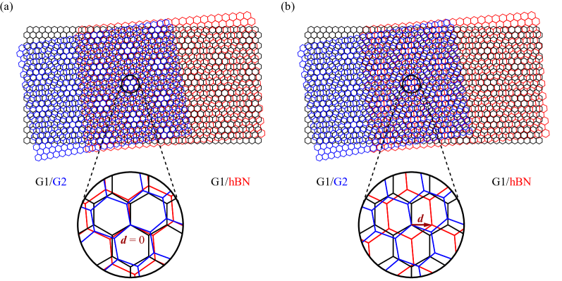
Figure 2: Schematic illustration of two moiré patterns that differ by a rigid displacement $\displaystyle\boldsymbol{d}$ of the hBN layer of a commensurate tBG/hBN system: (a) $\displaystyle\boldsymbol{d}=0$; (b) $\displaystyle\boldsymbol{d}\neq 0$. As we see, the G1/hBN moiré pattern is shifted. The twist angles and lattice constant mismatches are exaggerated in this schematic.

II.2 tBG/hBN supermoiré structures

A supermoiré structure is formed when the two twist angles are displaced slightly away from a low-order commensurate point, i.e. when

$$\theta_{{\rm GG}}=\theta_{{\rm GG}}^{npq}+\delta\theta_{{\rm GG}},\quad\theta_{{\rm GBN}}=\theta_{{\rm GBN}}^{npq}+\delta\theta_{{\rm GBN}},$$ (4)

where $\displaystyle(\theta_{{\rm GG}}^{npq},\theta_{{\rm GBN}}^{npq})$ is the commensurate pair defined by the integer triplet $\displaystyle(n,p,q)$ defined in Eq. (1), and both $\displaystyle\delta\theta_{{\rm GG}}$ and $\displaystyle\delta\theta_{{\rm GBN}}$ are $\displaystyle\sim 0.01^{\circ}$. The period and orientation of the supermoiré pattern depend on both $\displaystyle\delta\theta_{{\rm GG}}$ and $\displaystyle\delta\theta_{{\rm GBN}}$.

For sufficiently large supermoiré periods, the supermoiré structure can be characterized in terms of local commensurate tBG/hBN systems with the shift parameter $\displaystyle\boldsymbol{d}$ varying slowly in space. We let $\displaystyle\boldsymbol{d}=0$ correspond to local AAA stacking at $\displaystyle\boldsymbol{r}=0$, since in the supermoiré case a global shift of the hBN layer $\displaystyle\boldsymbol{d}(\boldsymbol{r})\rightarrow\boldsymbol{d}(\boldsymbol{r})+\boldsymbol{d}_{0}$ does not affect the overall supermoiré pattern. This can be seen by noting that a shift of hBN causes a magnified shift of the G1/hBN moiré pattern, which in turn produces a further magnified shift of the supermoiré pattern, and this can be cancelled by a reselection of the origin.

The analysis in Appendix B shows that in the small twist angle limit the magnification factor from $\displaystyle\boldsymbol{d}$ to $\displaystyle\boldsymbol{r}$ is

$$\gamma\equiv\frac{|\boldsymbol{r}|}{|\boldsymbol{d}|}\approx\frac{n}{\left|n\delta\theta_{{\rm GBN}}-\left(pe^{i\pi/3}+qe^{2i\pi/3}\right)\delta\theta_{{\rm GG}}\right|},$$ (5)

and that when the supercell of the $\displaystyle(n,p,q)$ commensurate system contains $\displaystyle N$ moiré cells of tBG, the ratio $\displaystyle r_{a}$ between the supermoiré lattice constant $\displaystyle a_{\rm sm}$ and the hBN lattice constant $\displaystyle a_{\rm BN}$ is

$$r_{a}\equiv\frac{a_{\rm sm}}{a_{\rm BN}}=\frac{\gamma}{\sqrt{N}}.$$ (6)

For supermoirés near $\displaystyle 60^{\circ}$, $\displaystyle 120^{\circ}$ and $\displaystyle 90^{\circ}$ commensurate points,

$$r_{a}^{120^{\circ},60^{\circ}}=\frac{1}{\sqrt{\delta\theta_{{\rm GG}}^{2}+\delta\theta_{{\rm GBN}}^{2}\pm\delta\theta_{{\rm GG}}\delta\theta_{{\rm GBN}}}}$$ (7)

with the $\displaystyle+$ sign for $\displaystyle 120^{\circ}$, and

$$r_{a}^{90^{\circ}}=\frac{1}{\sqrt{3\delta\theta_{{\rm GG}}^{2}+4\delta\theta_{{\rm GBN}}^{2}}}.$$ (8)

III Electronic Properties

III.1 Model Hamiltonian

In this section we describe how we model tBG/hBN trilayers with arbitrary twist angles $\displaystyle\theta_{{\rm GG}}$ and $\displaystyle\theta_{{\rm GBN}}$ and hBN layer translations $\displaystyle\boldsymbol{d}$. We adopt the commonly employed non-interacting model Hamiltonian, focusing on one valley since the other valley can be easily obtained by time reversal. The low-energy degrees of freedom are entirely in the graphene bilayer, but have a periodic contribution due to the adjacent hBN layer that we separate by writing

$$H(\boldsymbol{d})=H_{\rm tBG}+V_{\rm BN}(\boldsymbol{d}).$$ (9)

The bilayer has four $\displaystyle\pi$-electron sublattices counting the two honeycomb layers. For $\displaystyle H_{\rm tBG}$ we use the well-known four-sublattice continuum model Hamiltonian of tBG, Bistritzer and MacDonald (2011) adding a gate-controlled interlayer potential difference $\displaystyle U$. We adopt the ab initio estimates for the same and different sublattice interlayer tunneling parameters in tBG by setting $\displaystyle w_{AB}=113\rm meV$ Jung et al. (2014) and $\displaystyle w_{AA}/w_{AB}=0.8$, a value that accounts approximately for lattice relaxation. Carr et al. (2019)

In Eq. (9) we assume that $\displaystyle V_{\rm BN}(\boldsymbol{d})$ is non-zero only on G1 layer and not on G2. $\displaystyle V_{\rm BN}(\boldsymbol{d})$ can be separatedJung et al. (2014) into a spatially averaged term that is independent of position, and a periodic contribution:

$$V_{\rm BN}(\boldsymbol{d})=\sum_{\boldsymbol{k}}\left(\psi_{1\boldsymbol{k}}^{\dagger}(m_{0}\sigma^{z})\psi_{1\boldsymbol{k}}+\sum_{j=1}^{6}\psi_{1\boldsymbol{k}}^{\dagger}V_{j}(\boldsymbol{d})\psi_{1(\boldsymbol{k}+\boldsymbol{g}_{j})}\right).$$ (10)

The first term on the right hand side (RHS) of Eq. (10) captures the critical broken inversion symmetry in the G1 layer, as discussed in previous work. Zhang et al. (2019b); Bultinck et al. (2020); Wu and Das Sarma (2020); Repellin et al. (2020); Zhu et al. (2020b); Alavirad and Sau (2019); Chatterjee et al. (2020); Zhang et al. (2020) Ab initio calculations of monolayer graphene/hBN with full lattice relaxation yield the estimate $\displaystyle m_{0}=3.62\rm meV$, Jung et al. (2017) but experiments suggest that $\displaystyle m_{0}$ is significantly larger, Kim et al. (2018) possibly as large as $\displaystyle\sim 15\rm meV$ Hunt et al. (2013) and possibly reflecting many-body physics that is absent in the DFT calculation.Song et al. (2013) Since it is unclear whether many-body enhancement of $\displaystyle m_{0}$ is also important in tBG/hBN, we take $\displaystyle m_{0}=3.62\rm meV$ in most of our explicit calculations, using the value $\displaystyle m_{0}=10\rm meV$ in some calculations for comparison purposes.

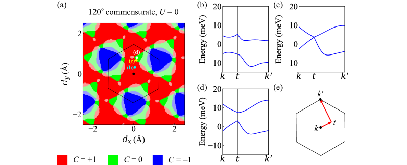
Figure 3: (a) Map of valence band Chern number $\displaystyle C$ vs. hBN displacement $\displaystyle\boldsymbol{d}$ for a $\displaystyle 120^{\circ}$ commensurate tBG/hBN moiré superlattice with zero interlayer potential difference $\displaystyle U$. Different colors specify different Chern numbers, as ilustrated by the legend below. The lighter shades identify semimetal regions with a gap closing that is indirect in momentum space. The black hexagon is the Wigner-Seitz cell of the hBN layer. (b)-(d) Band structures of the system at the $\displaystyle\boldsymbol{d}$ values marked by cyan (b), yellow (c) and white (d) dots in map (a). The band structures are plotted along the red path shown in (e), which includes the point $\displaystyle t$ at which the band touching occurs in (c). Band touching always occurs at some point in the mBZ along the map’s Chern number region boundaries.

The second term on the RHS of Eq. (10) accounts for the G1/hBN moiré pattern. The 6 transfer momenta $\displaystyle\boldsymbol{g}_{j}$ are from the first shell of the moiré reciprocal lattices and the $\displaystyle V_{j}$’s are matrices that act on sublattice degrees of freedom. Ab initio calculation Jung et al. (2017) estimate that all $\displaystyle V_{j}$’s are $\displaystyle\sim 10\rm meV$. These matrices are detailed in Appendix C. We capture the $\displaystyle\boldsymbol{d}$ dependence of the hopping matrix $\displaystyle V_{j}$ by multiplying the Fourier expansion coefficients by phase factors:

$$V_{j}(\boldsymbol{d})=V_{j}(0)e^{i\boldsymbol{g}_{j}\cdot\boldsymbol{d}_{M}},$$ (11)

where the shift $\displaystyle\boldsymbol{d}_{M}$ of the G1/hBN moiré pattern depends on $\displaystyle\boldsymbol{d}$ via Eq. (3).

III.2 Anomalous Hall effect at commensurate twist-angle pairs and supermoiré

Figure 3 (a) contains a map of the valence band Chern number $\displaystyle C$ vs. $\displaystyle\boldsymbol{d}$ for the $\displaystyle 120^{\circ}$ commensurate tBG/hBN trilayer implied by the model Hamiltonian described above with $\displaystyle U=0$. The Chern numbers were calculated using the highly efficient method described in Ref. Fukui et al., 2005. The structure present in the Chern number map demonstrates that band crossings occur as $\displaystyle\boldsymbol{d}$ is varied. In Figs. 3 (b)-(d) we plot the band structures at the $\displaystyle\boldsymbol{d}$ points highlighted in Fig. 3 (a). The expected band inversion at the Chern number boundary is apparent in these figures. We emphasize that if the $\displaystyle\boldsymbol{g}_{j}\neq 0$ terms in Eq. (10) were neglected, then the spectrum would be independent of $\displaystyle\boldsymbol{d}$, and the Chern number map would be monochromatic. The interesting structure is present only because the G1/hBN moiré pattern has a qualitative influence on electronic structures.

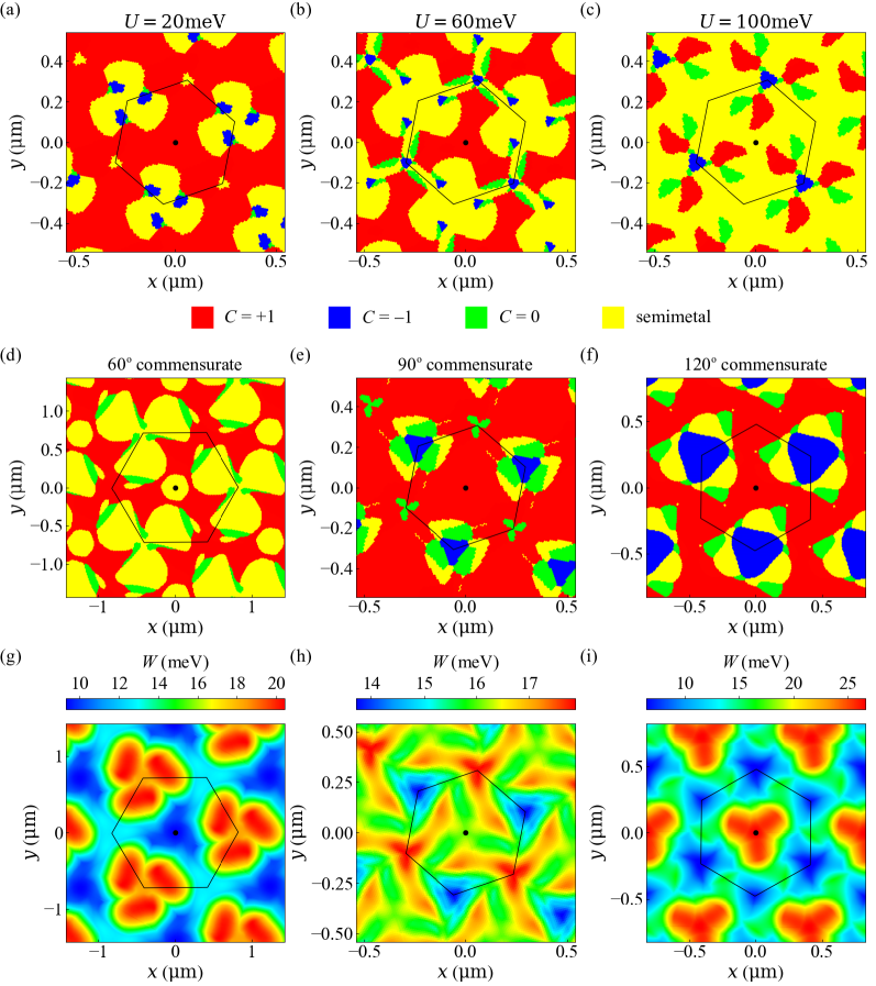
Figure 4: (a)-(c) Phase maps of a supermoiré structure close to the $\displaystyle 90^{\circ}$ commensurate twist point with $\displaystyle\delta\theta_{{\rm GG}}=\delta\theta_{{\rm GBN}}=0.01^{\circ}$, under various interlayer potential differences $\displaystyle U$. Different colors specify different phases, as illustrated by the legend on the bottom. $\displaystyle C$ is the valence band Chern number. The black hexagon is the Wigner-Seitz cell of the supermoiré pattern. At $\displaystyle U=20\rm meV$ the $\displaystyle C=+1$ phase is globally connected, indicating an overall measurable QAH effect. Otherwise the quantum Hall conductance is not quantized and the longitudinal conductivity is non-zero. (d)-(f) Phase maps of a supermoiré structure with $\displaystyle\delta\theta_{{\rm GG}}=\delta\theta_{{\rm GBN}}=0.01^{\circ}$ near (d) $\displaystyle 60^{\circ}$ commensurate; (e) $\displaystyle 90^{\circ}$ commensurate; (f) $\displaystyle 120^{\circ}$ commensurate structures, with $\displaystyle U=-20\rm meV$. All three cases have percolating $\displaystyle C=1$ phases. (g)-(i) Maps of the local conduction band width $\displaystyle W$ of the same systems as in (d)-(f). For $\displaystyle 90^{\circ}$ commensurate, $\displaystyle W$ refers to the difference between the top of the highest miniband and the bottom of the lowest miniband split from the conduction band of tBG. In a Stoner approximation spontaneous valley polarization occurs when an exchange interaction parameter exceeds $\displaystyle W$.

When the electronic structure of a supermoiré system is described in a local band picture, the $\displaystyle C(\boldsymbol{d})$ map in Fig. 3 (a) expands to a spatial map $\displaystyle C(\boldsymbol{r})=C(\boldsymbol{d}(\boldsymbol{r}))$ with magnification factor $\displaystyle\gamma$ defined in Eq. (5). When narrow bands lead to spontaneous valley polarization at odd moiré band fillings, Nomura and MacDonald (2006); Xie and MacDonald (2020); Zhu et al. (2020b); Saito et al. (2020a) spatial regions with different valley-dependent Chern numbers will have topologically distinct QAH or trivial phases. We notice that at some $\displaystyle\boldsymbol{d}$’s the valence and conduction bands overlap, giving rise to semimetal regions that cannot support a quantized Hall conductance, but can in principle support spontaneous valley polarization and therefore non-zero Hall effects. The entire supermoiré structure is therefore expected to support a complex spatially inhomogenous state containing alternating Chern insulator, trivial insulator, and semimetal phases. Several samples of such patterns are plotted in Fig. 4 (a)-(f). We see that at certain interlayer potential differences $\displaystyle U$, the $\displaystyle C=1$ phase or the semimetal phase percolates, while at other $\displaystyle U$’s no phase percolates. The percolation properties of different $\displaystyle U$’s are summarized in Table 1, where we see that percolation of the $\displaystyle C=1$ phase is most common in nearly $\displaystyle 120^{\circ}$ commensurate systems. If many-body effects do enhance $\displaystyle m_{0}$ or the single-particle sublattice splitting term in the Hamiltonian is larger than the estimate employed for these plots, more $\displaystyle C=1$ percolation is expected because the original gap opened by the $\displaystyle m_{0}$ term of the hBN potential is then larger and less easily inverted by either $\displaystyle U$ or the $\displaystyle\boldsymbol{g}\neq 0$ terms of the G1/hBN moiré potential. This observation is quantified in Appendix D where the corresponding results for $\displaystyle m_{0}=10\rm meV$ are summarized.

Table 1: Summary of percolating supermoiré phases of different commensurate structures under various interlayer potential difference $\displaystyle U$. S labels percolating semimetal states; X labels states with no percolating phase.

$\displaystyle U$ (meV)	$\displaystyle-100$	$\displaystyle-80$	$\displaystyle-60$	$\displaystyle-40$	$\displaystyle-20$	0	20	40	60	80	100
$\displaystyle 60^{\circ}$ commensurate	S	S	$\displaystyle C=1$	$\displaystyle C=1$	$\displaystyle C=1$	X	X	S	S	S	S
$\displaystyle 90^{\circ}$ commensurate	S	X	X	X	$\displaystyle C=1$	$\displaystyle C=1$	$\displaystyle C=1$	X	X	X	S
$\displaystyle 120^{\circ}$ commensurate	$\displaystyle C=1$	$\displaystyle C=1$	$\displaystyle C=1$	$\displaystyle C=1$	$\displaystyle C=1$	$\displaystyle C=1$	$\displaystyle C=1$	X	X	$\displaystyle C=1$	$\displaystyle C=1$

So far we have assumed full valley polarization. In practice valley polarization occurs only if the bands are sufficiently narrow relative to interaction strength. In Figs. 4 (g)-(i) we map the conduction band width $\displaystyle W$ vs. position $\displaystyle\boldsymbol{r}$. It follows from the Stoner mean-field criterion that spontaneous valley polarization is likely to be absent when the bandwidth $\displaystyle W$ exceeds the relevant exchange energy $\displaystyle X$. Self-consistent Hartree-Fock calculations in previous work suggest that $\displaystyle X\approx 30\rm meV$ in tBG with twist angle $\displaystyle\theta_{{\rm GG}}=1.1^{\circ}$ at moiré band filling factor $\displaystyle\nu=1$. Xie and MacDonald (2020) Since Hartree-Fock calculations tends to overestimate the exchange energy, our $\displaystyle W(\boldsymbol{r})$ maps may imply that some valley unpolarized regions, within which the anomalous Hall conductivity vanishes, may occur in the supermoiré pattern. (If the number $\displaystyle N$ of tBG moiré cells in a supercell of the commensurate system is a multiple of 4, for example in the $\displaystyle 90^{\circ}$ commensurate case, it is not impossible that the Fermi level could lie within one of the subband gaps of the original moiré bands.) According to the results shown in Fig. 4 (d)-(i), unpolarized states are more likely in semimetal phases of nearly $\displaystyle 60^{\circ}$ commensurate systems and in $\displaystyle C=1$ regions in nearly $\displaystyle 120^{\circ}$ commensurate systems.

III.3 Supermoiré quantum anomalous Hall effect twist angle windows

Our percolation-like Trugman (1983); Chalker and Coddington (1988) picture of the supermoiré anomalous Hall effect allows the spatial maps in Fig. 4 to be interpreted using a Landauer-büttiker transport picture. Büttiker (1986); Wang et al. (2013) In this picture an overall quantized anomalous Hall conductance occurs only when (i) a topologically nontrivial QAH phase percolates; (ii) the edge states between phase boundaries are sufficiently localized that their coupling can be neglected. The latter condition requires that the twist angle pair should be sufficiently close to a commensurate point that the supermoiré period is large compared to the lateral localization of the edge states. These considerations lead to the conclusion that there is a region of finite area in twist angle space surrounding each commensurate point within which the QAH effect can occur. Below we provide an estimate of the sizes of these twist angle windows.

We estimate the lateral localization width $\displaystyle\lambda$ of the edge states localized along boundaries between topologically nontrivial and trivial phases by concentrating on the two crossing levels and appealing to a Jackiw-Rebbi picture Jackiw and Rebbi (1976); Su et al. (1979) of two-dimensional Dirac fermions with a mass gap that varies smoothly with position. This mapping yields

$$\lambda=2\sqrt{\frac{v_{F}}{|\nabla_{\boldsymbol{r}}\Delta|}},$$ (12)

where $\displaystyle\Delta$ is the local gap. The typical Fermi velocity, $\displaystyle\hbar v_{F}\approx 100\rm{meV\cdot nm}$, was estimated from our model calculations by examining band dispersion at touching points like the one in Fig. 3 (c). Similarly the rate of variation of the gap with $\displaystyle\boldsymbol{d}$ is $\displaystyle|\nabla_{\boldsymbol{d}}\Delta|\approx 300\rm{meV}\cdot\rm{nm}^{-1}$. For a supermoiré lattice with a magnification factor $\displaystyle|\boldsymbol{r}|/|\boldsymbol{d}|=\gamma$, we have $\displaystyle|\nabla_{\boldsymbol{r}}\Delta|=|\nabla_{\boldsymbol{d}}\Delta|/\gamma$. Quantization is accurate when the edge-isolation parameter $\displaystyle\rho\equiv a_{\rm sm}/\lambda$, the ratio of gapped state size to edge state localization length, is large. From Eqs. (6) and (12) we find that when the twist angle is tuned toward a commensurate point defined by Eq. (1) with $\displaystyle n=p+q$,

$$\rho=\frac{a_{\rm sm}}{\lambda}=\frac{a_{\rm BN}}{2}\sqrt{\frac{\gamma|\nabla_{\boldsymbol{d}}\Delta|}{Nv_{F}}},$$ (13)

where $\displaystyle N=n^{2}$. Since the magnification factor $\displaystyle\gamma$ depends smoothly on twist angle, Eq. (13) implies that edge isolation will be achieved over smaller ranges of twist angle near higher order (larger $\displaystyle N$) commensuration points. Here we have assumed that both $\displaystyle v_{F}$ and $\displaystyle|\nabla_{\boldsymbol{d}}\Delta|$ retain their order of magnitude as $\displaystyle n$ becomes large. The latter assumption is justified by Eq. (11) since

$$|\nabla_{\boldsymbol{d}}\Delta|\sim|\nabla_{\boldsymbol{d}}V_{\rm BN}|\sim\left|i\boldsymbol{g}_{j}\cdot(\nabla_{\boldsymbol{d}}\boldsymbol{d}_{M})V_{j}(\boldsymbol{d})\right|\sim G_{\rm BN}V_{\rm BN},$$

where $\displaystyle G_{\rm BN}$ is the magnitude of primitive reciprocal lattice vector of the hBN, which does not change with $\displaystyle n$.

We adopt the practical numerical criterion that the Hall conductance is effectively quantized when the edge isolation parameter $\displaystyle\rho$ exceeds 5, which according to Eq. (13) is equivalent to $\displaystyle\gamma>500n^{2}$ ($\displaystyle r_{a}>500n$). From Eq. (5), the linear size of twist angle window that satisfies this criterion is $\displaystyle\delta\theta\approx 1/\gamma\approx 0.1^{\circ}/n^{2}$. The quantization windows for the series of twist angle windows up to $\displaystyle n=4$ are illustrated schematically in Fig. 5. Within the largest two of these windows, the typical supermoiré period is $\displaystyle\sim 0.1\sim$\displaystyle 1\text{\,}\mathrm{\SIUnitSymbolMicro m}$$, compared to typical tBG/hBN device sizes that are up to tens of micrometers. Sharpe et al. (2019); Serlin et al. (2020); Tschirhart et al. (2020) These considerations imply that devices can in principle be fabricated with up to tens of supermoiré periods on a side.

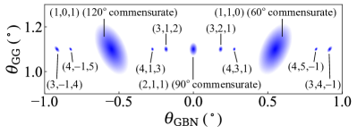
Figure 5: Twist angle windows for QAH effects according to criteria explained in the main text. Quantized regions are shaded blue and labeled by their $\displaystyle(n,p,q)$ integer triplets. The windows are larger for low-order commensurate twist angle pairs.

III.4 Anomalous Hall effect of incommensurate tBG/hBN

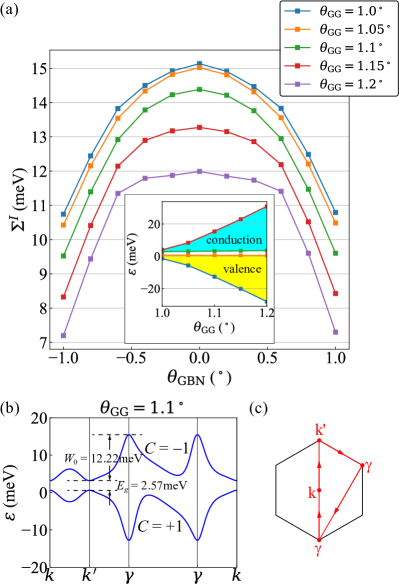
Figure 6: (a) Disorder self-energy $\displaystyle\Sigma^{I}$ due to the G1/hBN moiré potential vs. $\displaystyle\theta_{{\rm GBN}}$ for a series of $\displaystyle\theta_{{\rm GG}}$ values with $\displaystyle m_{0}=3.62\rm meV$ and interlayer potential difference $\displaystyle U=0$. Inset: the energy range of valence (yellow) and conduction (cyan) bands of near-magic angle tBG with sublattice symmetry broken by the $\displaystyle m_{0}$ term of the G1/hBN potential and the same value of $\displaystyle m_{0}$. (b) A sample tBG moiré band structure with $\displaystyle m_{0}=3.62$ meV, plotted along the red path shown in (c). The band Chern numbers $\displaystyle C$, the bandgap $\displaystyle E_{g}$, and the conduction band width $\displaystyle W_{0}$ in the absence of disorder are specified.

In principle all twist angle pairs are close to some commensurate point, just as all real numbers are near some rational number. However, most of these points have extremely large $\displaystyle n$ and can be practically viewed as incommensurate. In such a system, the moiré bands are broadened by the G1/hBN moiré, or split into an extremely large number of minibands. To roughly assess the influence of the G1/hBN moiré on electronic structures in this limit we adopt a simplified picture by treating it as a disorder potential with a scattering rate estimated using a self-consistent Born approximation:

$$\tau^{-1}_{n\boldsymbol{k}}=\frac{2\Sigma_{n\boldsymbol{k}}^{I}}{\hbar}=\frac{2\pi}{\hbar}\sum_{m}\sum_{j=1}^{6}\left|\left\langle{n\boldsymbol{k}}\right|V_{\rm BN}\left|{m(\boldsymbol{k}+\boldsymbol{g}_{j})}\right\rangle\right|^{2}\frac{1}{\pi}\frac{\Sigma_{m(\boldsymbol{k}+\boldsymbol{g}_{j})}^{I}}{(\epsilon_{m(\boldsymbol{k}+\boldsymbol{g}_{j})}-\epsilon_{n\boldsymbol{k}})^{2}+(\Sigma_{m(\boldsymbol{k}+\boldsymbol{g}_{j})}^{I})^{2}}.$$ (14)

Here $\displaystyle\Sigma_{n\boldsymbol{k}}^{I}$ is the imaginary part of the self energy, $\displaystyle\left|{n\boldsymbol{k}}\right\rangle$ is the Bloch state of the $\displaystyle n$th band at wave vector $\displaystyle\boldsymbol{k}$ and $\displaystyle\epsilon_{n\boldsymbol{k}}$ is the corresponding band energy, and the $\displaystyle\boldsymbol{g}_{j}$’s are from the first shell of G1/hBN moiré pattern. To simplify this approximation, we include only the moiré flat bands and assume that the scattering rate is approximately the same for all states by letting $\displaystyle\Sigma_{n\boldsymbol{k}}^{I}\to\Sigma^{I}$ in Eq. (14). This yields

$$\sum_{n,m=v,c}\frac{1}{N_{\boldsymbol{k}}}\sum_{\boldsymbol{k}\in\rm mBZ}\sum_{j=1}^{6}\frac{\left|\left\langle{n\boldsymbol{k}}\right|V_{\rm BN}\left|{m(\boldsymbol{k}+\boldsymbol{g}_{j})}\right\rangle\right|^{2}}{(\epsilon_{m(\boldsymbol{k}+\boldsymbol{g}_{j})}-\epsilon_{n\boldsymbol{k}})^{2}+(\Sigma^{I})^{2}}=1,$$ (15)

where $\displaystyle v$ and $\displaystyle c$ stand respectively for valence and conduction bands. We solve Eq. (15) for the disorder energy broadening $\displaystyle\Sigma^{I}$ using an $\displaystyle N_{\boldsymbol{k}}=50\times 50$ mesh to perform the momentum space integral and a numerical bisection method to fix $\displaystyle\Sigma^{I}$.

Figure 6 (a) shows disorder self-energy $\displaystyle\Sigma^{I}$ of the tBG bands calculated in this way and compares them with the disorder-free band widths $\displaystyle W$ and gaps shown in the inset. The disorder broadening is largest when the moiré bands are narrowest, as expected on the basis of density-of-states considerations, and exceeds $\displaystyle 10{\rm meV}$ over a broad range of twist angles. Within a Stoner mean-field picture, spontaneous valley polarization is expected only when the moiré band width is smaller than the exchange energy strength. Assuming that the disorder self-energy $\displaystyle\Sigma^{I}$ effectively adds to the band width, the values reported in Fig. 6 suggest that spontaneous valley polarization is unlikely in incommensurate tBG/hBN. Since the disorder broadening effect is in any case sufficient to close the typically $\displaystyle 2\sim 3$meV band gap present when the G1/hBN moiré pattern is ignored, even if present spontaneous valley polarization is unlikely to produce a quantized anomalous Hall effect. The property that an incommensurate tBG/hBN interaction can be strong enough to close gaps is consistent with our findings for commensurate systems. As also in that case a larger value for $\displaystyle m_{0}=10\rm meV$ would imply more quantum anomalous Hall effects that are more, but still imperfectly, persistent. (see Appendix D)

IV Discussion

When tBG/hBN devices are fabricated, $\displaystyle\theta_{{\rm GG}}$ can be accurately controlled to a precision of order of $\displaystyle\sim 0.1^{\circ}$ because the two graphene sheets are extracted from a common exfoliated single-layer crystal.Kim et al. (2016) This advantage is not present when aligning the graphene and hBN layers and $\displaystyle\theta_{{\rm GBN}}$ is therefore far less precisely controlled. Nominally aligned samples may have differences in orientation in the range of $\displaystyle\sim\pm 1^{\circ}$. If the orientation angle is random within this range, the two moiré patterns will generally be incommensurate and therefore, we have argued, likely to show only a weak or zero anomalous Hall effect. If by chance $\displaystyle\theta_{{\rm GBN}}$ falls into one of the twist angle windows identified in Fig. 5, devices are likely to exhibit a quantized Hall conductance. Close to these twist angle windows the Hall conductance is likely to be large, but still not quantized. This provides a possible explanation for the fact that accurately quantized Hall conductances seem to be observed relatively rarely in experiments on tBG/hBN. Our expectation that the Hall conductance is more likley to be quantized for twist angle pairs closer to a commensurate point is consistent with the experimental observation of a quantized Hall resistance in a sample with measured twist angles $\displaystyle\theta_{{\rm GG}}\approx 1.15^{\circ}$ and $\displaystyle\theta_{{\rm GBN}}\approx\pm 0.6^{\circ}$, Serlin et al. (2020) which is close to either the $\displaystyle 60^{\circ}$ or the $\displaystyle 120^{\circ}$ commensurate point depending on the sign of $\displaystyle\theta_{{\rm GBN}}$, and a non-quantized Hall resistance in a sample with $\displaystyle\theta_{{\rm GG}}\approx 1.2^{\circ}$ and $\displaystyle\theta_{{\rm GBN}}\approx\pm 0.8^{\circ}$, Sharpe et al. (2019) which is further from a commensurate twist-angle-pair point.

Since there will always be a difference in local lattice bonding energy per area between regions with different values of the hBN sliding vector $\displaystyle\boldsymbol{d}$, a supermoiré structure will spontaneously expand regions in which $\displaystyle\boldsymbol{d}$ is close to the most energetically preferred value. Woods et al. (2014) For samples smaller than a supermoiré period, this process will induce relaxation towards a uniform phase with the energetically preferred value of $\displaystyle\boldsymbol{d}$. At present we do not know whether or not these uniform samples are more likely to be Chern insulators, trivial insulators or semimetals.

In larger samples, the supermoiré pattern can introduce intrinsic inhomogeneity at the micrometer scale. One consequence is that the measured Hall conductance can be a device-specific quantity, even for devices that have the same twist angles. This scenario is consistent with the fact that in some devices the quantum anomalous Hall effect is observed Serlin et al. (2020) for some source, drain and voltage contact choices and not for others. The observation of domain walls Tschirhart et al. (2020) that remain pinned even when the magnetization has apparently saturated is also consistent with device scale inhomogeneity. Persistent pinning might be associated with local absence of valley polarization as discussed in Sec. III.2.

The relationship we propose between commensurability and the appearance of the QAH effect in tBG/hBN could be tested by measuring the twist-angle-pair of a nearly commensurate device using Bragg interferometry. Kazmierczak et al. (2020) In this technique a high-energy electron beam with sub-moiré size is rastered through and diffracted by both graphene and hBN layers. In tBG, the intensity of the Bragg disks varies with electron-injection position with moiré periodicity as a result of spatially varying interference between the two graphene layers. For nearly commensurate tBG/hBN, we expect this periodicity to be further modulated with a larger periodicity, namely the supermoiré, by a perturbation from the hBN layer.

The absence of an anomalous Hall effect in a large device could signal the absence of valley polarization at any point, or a complex valley-polarization domain structure. These circumstances can be distinguished in principle by using nano-ARPES Bostwick et al. (2012); Dudin et al. (2010) to separately detect energy and momentum distribution functions in opposite valleys to see if they are different.Zhu et al. (2020d) Valley polarization can also be measured locally by looking for valley-contrasting optical properties.Wehling et al. (2015); Hipolito and Pereira (2017); Mak et al. (2018)

V Summary and Conclusions

Trilayer van der Waals heterojunctions have two independent relative twist angles. We have identified a series of $\displaystyle(\theta_{{\rm GG}},\theta_{{\rm GBN}})$ twist-angle pairs in tBG/hBN trilayer systems at which the graphene/graphene and graphene/hBN moiré periodicities are commensurate and $\displaystyle\theta_{{\rm GG}}$ is close to the magic angle at which isolated tBG moiré bands are narrow and support strong correlation physics. We use a non-interacting continuum model Hamiltonian that accounts for both moiré patterns to address the trilayer electronic properties. Although the active degrees of freedom are localized in the two graphene layers, the hBN layer produces an effective external potential that includes both a position independent term, and a position-dependent term that is often ignored.Zhang et al. (2019b); Bultinck et al. (2020); Wu and Das Sarma (2020); Repellin et al. (2020); Zhu et al. (2020b); Alavirad and Sau (2019); Chatterjee et al. (2020); Zhang et al. (2020) We find that when the position-dependent terms are retained, the band structures and Chern numbers of commensurate trilayers change as the hBN layer is rigidly displaced by translation vector $\displaystyle\boldsymbol{d}$. When only the translationally invariant mass term are included in the Hamiltonian, the electronic structure is $\displaystyle\boldsymbol{d}$-independent, and the Chern number maps are uniform at $\displaystyle C=1$. This finding proves that the role of the position-dependent terms in trilayers, which have the periodicity of the graphene/hBN moiré, is essential.

Building on this result, we analyze the role of the graphene/hBN moiré in tBG/hBN trilayers, focusing on their importance for the appearance or absence of the QAH effect at odd integer moiré band fillings. When the twist angle pair is close to a commensurate point, a long-period supermoiré pattern is formed that can be viewed as a slow spatial variation of the hBN translation vector $\displaystyle\boldsymbol{d}$. When analyzed using a local moiré band picture, the supermoiré at odd integer moiré band filling factors is characterized by a spatial map of distinct states, including correlated insulating states with various Chern numbers, semimetal states, and valley-unpolarized states. We argue that an overall QAH state is possible only when a topologically nontrivial insulating phase percolates and the twist angle pair is close enough to a commensurate value. For twist angles far from commensurate points, we assume that the hBN moiré potential acts like a disorder potential which we treat using a self-consistent Born approximation. We argue that that the anomalous Hall effect is unlikely to occur in this regime because of the disorder-induced band-broadening effect.

Our proposal can explain the experimental observation of both quantized and non-quantized anomalous Hall effects, as well as states with no anomalous Hall effect at all, in tBG/hBN samples. The supermoiré picture also provides possible interpretations of unexplained inhomogeneities observed in some experiments that act as pinning centers of orbital ferromagnetism. Direct verification of our proposal could be achieved by performing Bragg interferometry moiré structure and transport measurements in the same sample.

Earlier experimental Wang et al. (2019b); Finney et al. (2019); Wang et al. (2019a); Tsai et al. (2019) and theoretical Leconte and Jung (2019); Andelkovic et al. (2020); Amorim and Castro (2018); Zhu et al. (2020c, a) work has addressed the rich electronic properties of other trilayer systems, including hBN/graphene/hBN trilayers and twisted trilayer graphene system. This manuscript shows that the tBG/hBN trilayer system is also an attractive platform to study bi-moiré electronic structures, and to study the interplay between strong-correlations and quasiperiodicity.

Note added in proof — As this manuscript was being prepared we noticed a related preprint Lin et al. (2020) that identifies a series of commensurate twist angle pairs in tBG/hBN and performed full structural relaxation calculations. This work supports our speculation that commensurate moiré structures are likely to be energetically preferred. A second related preprint Mao and Senthil (2020) has identified the two simplest examples of morié commensurability, and provides a complementary analysis of the electronic properties of incommensurate tBG/hBN.

Appendix A Exact geometry of general commensurate tBG/hBN trilayers

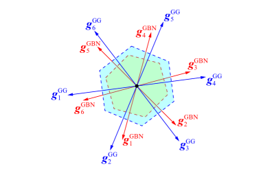
Figure A1: The primitive reciprocal lattice vectors of the G1/G2 (blue) and G1/hBN moiré patterns (red).

The commensurability of the tBG/hBN trilayer is captured by the fact that any reciprocal lattice vector of either moiré pattern is a linear combination of the primitive basis of a common mini- reciprocal lattice with integer coefficients. This is equivalent to saying that any reciprocal lattice vector of one moiré pattern is a linear combination of the reciprocal basis of the other moiré pattern with rational coefficients. According to this condition we can set

$$\boldsymbol{g}_{1}^{\rm GBN}=\tilde{p}\boldsymbol{g}_{2}^{\rm GG}+\tilde{q}\boldsymbol{g}_{3}^{\rm GG}$$ (16)

where $\displaystyle\boldsymbol{g}_{j}^{\rm GG}$ and $\displaystyle\boldsymbol{g}_{j}^{\rm GBN}$ are defined in Fig. A1, $\displaystyle\tilde{p}$ and $\displaystyle\tilde{q}$ are rational numbers with the least common denominator $\displaystyle n$ so that $\displaystyle\tilde{p}=p/n$ and $\displaystyle\tilde{q}=q/n$. Rotating both sides of Eq. (16) clockwise by $\displaystyle 90^{\circ}$ and scaling by $\displaystyle 1/\sqrt{3}$ yields Eq. (1) in the main text.

We now solve for the exact expression of the twist angle pair $\displaystyle(\theta_{{\rm GG}},\theta_{{\rm GBN}})$ in terms of $\displaystyle(\tilde{p},\tilde{q})$. We first write Eq. (1) in a complex number form in which 2D vectors are represented by complex numbers whose real and imaginary parts are the two components i.e. $\displaystyle\boldsymbol{K}_{1}=K$, $\displaystyle\boldsymbol{K}_{2}=Ke^{i\theta_{{\rm GG}}}$ and $\displaystyle\boldsymbol{K}_{\rm BN}=Ke^{i\theta_{{\rm GBN}}}/\alpha$. Rotation matrices are then represented by complex numbers with norm 1 i.e. $\displaystyle\mathcal{R}_{\phi}=e^{i\phi}$:

$$\frac{e^{i\theta_{{\rm GBN}}}}{\alpha}-1=\left(\tilde{p}e^{i\frac{\pi}{3}}+\tilde{q}e^{i\frac{2\pi}{3}}\right)(e^{i\theta_{{\rm GG}}}-1).$$ (17)

Adding $\displaystyle 1$ to each side of Eq. (17) and then multiplying by complex conjugates yields an equation for $\displaystyle\theta_{{\rm GG}}$ which has two exact solutions modulo $\displaystyle 2\pi$:

$$\theta_{{\rm GG}}^{\pm}=\arccos\frac{t}{\sqrt{t^{2}+s^{2}}}\pm\arccos\frac{t+\frac{1}{2}\left(1-\frac{1}{\alpha^{2}}\right)}{\sqrt{t^{2}+s^{2}}},$$ (18)

where $\displaystyle t=r^{2}+s^{2}-r$, $\displaystyle r=(\tilde{p}-\tilde{q})/2$ and $\displaystyle s=\sqrt{3}(\tilde{p}+\tilde{q})/2$. $\displaystyle\theta_{{\rm GG}}^{+}$ is typically not small enough to justify the continuum models that make the use of moiré periodic Hamiltonians. On the other hand $\displaystyle\theta_{{\rm GG}}^{-}$ is small since $\displaystyle\alpha$ is very close to 1.

By similar means we can also get an equation of $\displaystyle\theta_{{\rm GBN}}$ from Eq. (17), which has two exact solutions modulo $\displaystyle 2\pi$:

$$\theta_{{\rm GBN}}^{\pm}=\arccos\frac{r-1}{\sqrt{(r-1)^{2}+s^{2}}}\pm\arccos\frac{\alpha r-\frac{1}{2}\left(\alpha+\frac{1}{\alpha}\right)}{\sqrt{(r-1)^{2}+s^{2}}}.$$ (19)

Again, $\displaystyle\theta_{{\rm GBN}}^{+}$ is typically not small enough to justify moiré band theory.

The three special cases discussed in the main text are obtained by substituting $\displaystyle(\tilde{p},\tilde{q})=(1,0)$, $\displaystyle(0,1)$ and $\displaystyle(1/2,1/2)$ into Eqs. (18) and (19), and using $\displaystyle\alpha=1.017$. We obtain:

$$\theta_{{\rm GG}}^{60^{\circ}}=60^{\circ}-\arccos\left(1-\frac{1}{2\alpha^{2}}\right)\approx 1.103^{\circ},$$ (20)

$$\theta_{{\rm GBN}}^{60^{\circ}}=\frac{\theta_{{\rm GG}}^{60^{\circ}}}{2}=\arccos\left(\frac{1}{2\alpha}\right)-60^{\circ}\approx 0.551^{\circ},$$ (21)

$$\theta_{{\rm GG}}^{120^{\circ}}=30^{\circ}-\arccos\left(\frac{2}{\sqrt{3}}\left(1-\frac{1}{4\alpha^{2}}\right)\right)\approx 1.116^{\circ},$$ (22)

$$\theta_{{\rm GBN}}^{120^{\circ}}=-30^{\circ}+\arccos\left(\frac{1}{\sqrt{3}}\left(\alpha+\frac{1}{2\alpha}\right)\right)\approx-0.577^{\circ},$$ (23)

$$\theta_{{\rm GG}}^{90^{\circ}}=\arccos\sqrt{\frac{3}{7}}-\arccos\left(\frac{1}{\sqrt{21}}\left(5-\frac{2}{\alpha^{2}}\right)\right)\approx 1.106^{\circ},$$ (24)

$$\theta_{{\rm GBN}}^{90^{\circ}}=\arccos\left(\frac{1}{\sqrt{7}}\left(\alpha+\frac{1}{\alpha}\right)\right)-\arccos\frac{2}{\sqrt{7}}\approx-0.009^{\circ}.$$ (25)

Appendix B Geometry of tBG/hBN supermoiré

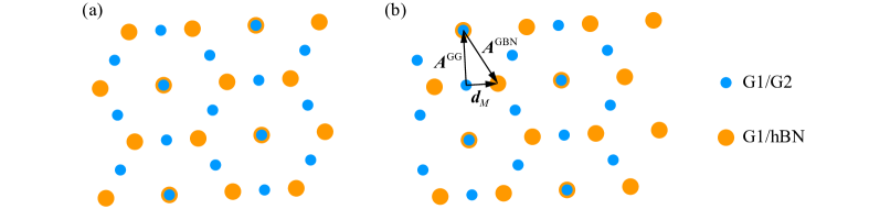
Figure A2: Local AA stacking points of the two moiré patterns in a $\displaystyle 90^{\circ}$ commensurate system: (a) $\displaystyle\boldsymbol{d}_{M}=0$; (b) $\displaystyle\boldsymbol{d}_{M}$ is the half of a shortest G1/hBN moiré lattice vector, which is the sum of a G1/G2 moiré lattice vector $\displaystyle\boldsymbol{A}^{\rm GG}$ and a G1/hBN moiré lattice vector $\displaystyle\boldsymbol{A}^{\rm GBN}$. The two systems are identical up to a translation. The small blue and large orange dots represent the local AA stacking points of G1/G2 and G1/hBN moiré patterns respectively.

For a tBG/hBN trilayer with twist angle pair $\displaystyle(\theta_{{\rm GG}},\theta_{{\rm GBN}})$, the two moiré Bravais lattices are defined by

$$\begin{cases}\boldsymbol{A}^{{\rm GG}}=\left(1-\mathcal{R}_{-\theta_{{\rm GG}}}\right)^{-1}\boldsymbol{a}\\ \boldsymbol{A}^{{\rm GBN}}=\left(1-\frac{\mathcal{R}_{-\theta_{{\rm GBN}}}}{\alpha}\right)^{-1}\boldsymbol{a}\end{cases}$$ (26)

where $\displaystyle\boldsymbol{a}$ is a lattice vector of the G1 graphene layer.

We start from an $\displaystyle(n,p,q)$ commensurate structure with $\displaystyle\boldsymbol{d}=0$, so that the two moiré patterns share AA stacking points at the origin, and look for other common AA stacking points $\displaystyle\boldsymbol{r}$ that satisfy

$$\boldsymbol{r}=\left(1-\mathcal{R}_{-\theta_{{\rm GG}}^{npq}}\right)^{-1}\boldsymbol{a}_{1}=\left(1-\frac{\mathcal{R}_{-\theta_{{\rm GBN}}^{npq}}}{\alpha}\right)^{-1}\boldsymbol{a}_{2},$$ (27)

where both $\displaystyle\boldsymbol{a}_{1}$ and $\displaystyle\boldsymbol{a}_{2}$ are G1 lattice vectors. Now we tune the twist angle pair slightly away by $\displaystyle(\delta\theta_{{\rm GG}},\delta\theta_{{\rm GBN}})$, and then the AA stacking points in both moiré patterns are shifted and their relative displacement is

$$\boldsymbol{d}_{M}(\boldsymbol{r})=\left(1-\frac{\mathcal{R}_{-\theta_{{\rm GBN}}}}{\alpha}\right)^{-1}\boldsymbol{a}_{2}-\left(1-\mathcal{R}_{-\theta_{{\rm GG}}}\right)^{-1}\boldsymbol{a}_{1},$$ (28)

where $\displaystyle\theta_{{\rm GG}}=\theta_{{\rm GG}}^{npq}+\delta\theta_{{\rm GG}}$ and $\displaystyle\theta_{{\rm GBN}}=\theta_{{\rm GBN}}^{npq}+\delta\theta_{{\rm GBN}}$. Writing $\displaystyle\boldsymbol{a}_{1}$ and $\displaystyle\boldsymbol{a}_{2}$ in Eq. (28) in terms of $\displaystyle\boldsymbol{r}$ using Eq. (27) yields an explicit expression for $\displaystyle\boldsymbol{d}_{M}(\boldsymbol{r})$, and then an explicit expression of $\displaystyle\boldsymbol{d}(\boldsymbol{r})$ by using Eq. (3). For small $\displaystyle\delta\theta_{{\rm GG}}$ and small $\displaystyle\delta\theta_{{\rm GBN}}$,

$$\boldsymbol{d}(\boldsymbol{r})=\left(\delta\theta_{{\rm GBN}}\mathcal{R}_{90^{\circ}}-\frac{\alpha}{n}\delta\theta_{{\rm GG}}\left(p\mathcal{R}_{30^{\circ}}+q\mathcal{R}_{-30^{\circ}}\right)\mathcal{R}_{\theta_{{\rm GBN}}^{npq}-\theta_{{\rm GG}}^{npq}}\right)\boldsymbol{r}.$$ (29)

To obtain this expression one needs to make use of the relation

$$n\left(1-\frac{\mathcal{R}_{\theta_{{\rm GBN}}^{npq}}}{\alpha}\right)=\left(p\mathcal{R}_{60^{\circ}}+q\mathcal{R}_{120^{\circ}}\right)\left(1-\mathcal{R}_{\theta_{{\rm GG}}^{npq}}\right).$$ (30)

which can be extracted directly from Eq. (1).

Further approximation neglecting the difference between $\displaystyle\mathcal{R}_{\theta_{{\rm GG}}^{npq}}$, $\displaystyle\mathcal{R}_{\theta_{{\rm GBN}}^{npq}}$, $\displaystyle\alpha$ and 1 yields

$$\boldsymbol{d}(\boldsymbol{r})\approx\left(\delta\theta_{{\rm GBN}}\mathcal{R}_{90^{\circ}}-\frac{1}{n}\delta\theta_{{\rm GG}}(p\mathcal{R}_{30^{\circ}}+q\mathcal{R}_{-30^{\circ}})\right)\boldsymbol{r}.$$ (31)

Take the norm of both sides of Eq. (31) and we get Eq. (5) in the main text.

To understand the factor $\displaystyle 1/\sqrt{N}$ in Eq. (6), we must return to the commensurate system and show that the system is invariant not only under a change of $\displaystyle\boldsymbol{d}$ by a lattice vector of the hBN, but also under a change of $\displaystyle\boldsymbol{d}$ by a lattice vector of a lattice that is $\displaystyle N$ times as dense as the hBN. We look at the shift of the position of G1/hBN moiré pattern, $\displaystyle\boldsymbol{d}_{M}$, due to the change in $\displaystyle\boldsymbol{d}$. The system is obviously invariant under a shift of $\displaystyle\boldsymbol{d}_{M}$ by any G1/hBN moiré lattice vector $\displaystyle\boldsymbol{A}^{{\rm GBN}}$, and in fact also invariant under a shift of the G1/hBN moiré pattern by any G1/G2 moiré lattice vector $\displaystyle\boldsymbol{A}^{{\rm GG}}$, which can be understood by noticing its equivalence to a shift of the G1/G2 moiré pattern by $\displaystyle-\boldsymbol{A}^{{\rm GG}}$. An example is shown in Fig. A2. We also notice that combining Eqs. (26) and (30) (note that we are dealing with commensurate systems so $\displaystyle\theta_{{\rm GG}}=\theta_{{\rm GG}}^{npq}$, $\displaystyle\theta_{{\rm GBN}}=\theta_{{\rm GBN}}^{npq}$) yields the relation between the two moiré Bravais lattices:

$$n\boldsymbol{A}^{{\rm GG}}=\left(p\mathcal{R}_{-60^{\circ}}+q\mathcal{R}_{-120^{\circ}}\right)\boldsymbol{A}^{{\rm GBN}}$$ (32)

which is identical to the relation between the two moiré reciprocal lattices characterized by Eq. (16), up to a mirror reflection. Since this relation folds the mBZ of the G1/G2 moiré pattern into $\displaystyle 1/N$ of its area, it also folds the spatial primitive cell of the G1/hBN moiré pattern into $\displaystyle 1/N$ of its area. Hence we conclude that the system is invariant under a shift of $\displaystyle\boldsymbol{d}_{M}$ by a lattice vector of a triangular lattice that is $\displaystyle N$ times as dense as the Bravais lattice of the G1/hBN pattern, which is equivalent to a shift of $\displaystyle\boldsymbol{d}$ by a lattice vector of a lattice that is $\displaystyle N$ times as dense as the hBN.

Appendix C Details of model Hamiltonian

The continuum model Hamiltonian of tBG Bistritzer and MacDonald (2011) in one microscopic valley with a tunable interlayer potential difference $\displaystyle U$ is

$$H_{\rm tBG}=\sum_{\boldsymbol{k}}\left(\psi_{1\boldsymbol{k}}^{\dagger}\left(-\frac{U}{2}+\hbar v\boldsymbol{\sigma}_{1}\cdot\boldsymbol{k}\right)\psi_{1\boldsymbol{k}}+\psi_{2\boldsymbol{k}}^{\dagger}\left(\frac{U}{2}+\hbar v\boldsymbol{\sigma}_{2}\cdot\boldsymbol{k}\right)\psi_{2\boldsymbol{k}}\right)+\left(\sum_{\boldsymbol{k}}\sum_{j=1}^{3}\psi_{1\boldsymbol{k}}^{\dagger}T_{j}\psi_{2(\boldsymbol{k}+\boldsymbol{q}_{j})}+\rm H.c.\right),$$ (33)

where $\displaystyle v\boldsymbol{\sigma}_{l}\cdot\boldsymbol{k}$ ($\displaystyle l=1,2$) is the graphene Dirac Hamiltonian of the $\displaystyle l$th layer, with $\displaystyle\boldsymbol{\sigma}_{1}=(\sigma^{x},\sigma^{y})$, $\displaystyle\boldsymbol{\sigma}_{2}=(\cos\theta_{{\rm GG}}\sigma^{x}-\sin\theta_{{\rm GG}}\sigma^{y},\sin\theta_{{\rm GG}}\sigma^{x}+\cos\theta_{{\rm GG}}\sigma^{y})$ and $\displaystyle v=10^{6}\rm m/s$.

$$T_{j}=\begin{pmatrix}w_{AA}&e^{-i\frac{2\pi}{3}(j-1)}w_{AB}\\ e^{i\frac{2\pi}{3}(j-1)}w_{AB}&w_{AA}\end{pmatrix}$$ (34)

are the three interlayer tunneling matrices where $\displaystyle w_{AB}=113\rm meV$ Jung et al. (2014) and $\displaystyle w_{AA}=0.8w_{AB}$. Carr et al. (2019) The vectors $\displaystyle\boldsymbol{q}_{j}$ are shown in Fig. 1 (b). Note that we have written the $\displaystyle T_{j}$ matrices in a convention taking a local AA-stacking point as the origin, which is different from Ref. Bistritzer and MacDonald, 2011 where AB-stacking is taken as the origin.

The hBN layer adds to the Hamiltonian the term $\displaystyle V_{\rm BN}$ specified in Eq. (10) in main text, where the 6 transfer momenta $\displaystyle\boldsymbol{g}_{j}$ are defined in Fig. 1 (b) for arbitrary $\displaystyle\theta_{{\rm GBN}}$. The transfer matrices $\displaystyle V_{j}$ depends on $\displaystyle\boldsymbol{d}$ via Eq. (11). $\displaystyle C_{3}$ symmetry requires that $\displaystyle V_{j}(0)$ has the following forms:

$$\displaystyle V_{1}(0)=V_{4}^{\dagger}(0)=\begin{pmatrix}C_{0}+C_{z}&C_{AB}\\ C_{AB}&C_{0}-C_{z}\end{pmatrix}$$ (35)

$$\displaystyle V_{3}(0)=V_{6}^{\dagger}(0)=\begin{pmatrix}C_{0}+C_{z}&e^{-i\frac{2\pi}{3}}C_{AB}\\ e^{i\frac{2\pi}{3}}C_{AB}&C_{0}-C_{z}\end{pmatrix}$$ (36)

$$\displaystyle V_{5}(0)=V_{2}^{\dagger}(0)=\begin{pmatrix}C_{0}+C_{z}&e^{i\frac{2\pi}{3}}C_{AB}\\ e^{-i\frac{2\pi}{3}}C_{AB}&C_{0}-C_{z}\end{pmatrix}$$ (37)

where $\displaystyle C_{0}$, $\displaystyle C_{z}$ and $\displaystyle C_{AB}$ are complex values with dimension of energy. Different ab initio results of these quantities as well as the mass term $\displaystyle m_{0}$ under various assumptions are presented in Refs. Jung et al., 2014, 2015, 2017. Here we use the most realistic one, “relaxed $\displaystyle\beta$” in Ref. Jung et al., 2017:

$$\begin{array}[]{c}m_{0}=3.62\rm meV\\ C_{0}=7.03e^{i(134.54^{\circ})}\rm meV\\ C_{z}=6.85e^{i(60.14^{\circ})}\rm meV\\ C_{AB}=12.94e^{i(-13.81^{\circ})}\rm meV\end{array}$$ (38)

Appendix D Results for larger mass term

Table 2: Summary of percolating supermoiré phases of different commensurate structures under various interlayer potential difference $\displaystyle U$, with $\displaystyle m_{0}=10\rm meV$. S labels percolating semimetal states; X labels states with no percolating phase.

$\displaystyle U$ (meV)	$\displaystyle-100$	$\displaystyle-80$	$\displaystyle-60$	$\displaystyle-40$	$\displaystyle-20$	0	20	40	60	80	100
$\displaystyle 60^{\circ}$ commensurate	$\displaystyle C=1$	$\displaystyle C=1$	$\displaystyle C=1$	$\displaystyle C=1$	$\displaystyle C=1$	$\displaystyle C=1$	$\displaystyle C=1$	$\displaystyle C=1$	$\displaystyle C=1$	S	S
$\displaystyle 90^{\circ}$ commensurate	$\displaystyle C=1$	$\displaystyle C=1$	$\displaystyle C=1$	$\displaystyle C=1$	$\displaystyle C=1$	$\displaystyle C=1$	$\displaystyle C=1$	$\displaystyle C=1$	$\displaystyle C=1$	X	S
$\displaystyle 120^{\circ}$ commensurate	$\displaystyle C=1$	$\displaystyle C=1$	$\displaystyle C=1$	$\displaystyle C=1$	$\displaystyle C=1$	$\displaystyle C=1$	$\displaystyle C=1$	$\displaystyle C=1$	$\displaystyle C=1$	$\displaystyle C=1$	$\displaystyle C=1$

Table 2 shows the percolating phase of tBG/hBN supermoiré structures with $\displaystyle m_{0}=10\rm meV$ and various interlayer potential difference $\displaystyle U$. The $\displaystyle C=1$ region nearly always percolates, except for very large $\displaystyle U$. Figure A3 shows the estimated broadening effect $\displaystyle\Sigma^{I}$ of the periodical part of the G1/hBN moiré potential on the tBG bands gapped by the spatially uniform sublattice asymmetric term with $\displaystyle m_{0}=10\rm meV$. The gap increases with $\displaystyle\theta_{{\rm GG}}$, ranging from $\displaystyle\sim 6\rm meV$ to $\displaystyle\sim 8\rm meV$ in the near-magic angle regime. The broadening effect is large enough to close the gap except for relatively large $\displaystyle\theta_{{\rm GG}}$ and relatively large $\displaystyle\theta_{{\rm GBN}}$. For larger $\displaystyle\theta_{{\rm GG}}$ the original bandwidth $\displaystyle W_{0}$ is large, thus the full bandwidth $\displaystyle W\sim W_{0}+\Sigma^{I}$ is very likely to destroy the valley polarization, resulting in zero anomalous Hall conductance. For smaller $\displaystyle\theta_{{\rm GG}}$ non-quantized anomalous Hall conductance is possible.

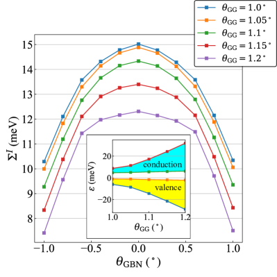
Figure A3: Disorder self-energy $\displaystyle\Sigma^{I}$ due to the G1/hBN moiré potential vs. $\displaystyle\theta_{{\rm GBN}}$ for a series of $\displaystyle\theta_{{\rm GG}}$ values with $\displaystyle m_{0}=10\rm meV$ and interlayer potential difference $\displaystyle U=0$. Inset: the energy range of valence (yellow) and conduction (cyan) bands of near-magic angle tBG with sublattice symmetry broken by the $\displaystyle m_{0}$ term of the G1/hBN potential and the same value of $\displaystyle m_{0}$.

References

- Bistritzer and MacDonald (2011) R. Bistritzer and A. H. MacDonald, Proc. Natl. Acad. Sci. 108, 12233 (2011).
- Cao et al. (2018a) Y. Cao, V. Fatemi, A. Demir, S. Fang, S. L. Tomarken, J. Y. Luo, J. D. Sanchez-Yamagishi, K. Watanabe, T. Taniguchi, E. Kaxiras, R. C. Ashoori, and P. Jarillo-Herrero, Nature 556, 80 (2018a).
- Sharpe et al. (2019) A. L. Sharpe, E. J. Fox, A. W. Barnard, J. Finney, K. Watanabe, T. Taniguchi, M. A. Kastner, and D. Goldhaber-Gordon, Science 365, 605 (2019).
- Serlin et al. (2020) M. Serlin, C. L. Tschirhart, H. Polshyn, Y. Zhang, J. Zhu, K. Watanabe, T. Taniguchi, L. Balents, and A. F. Young, Science 367, 900 (2020).
- Nuckolls et al. (2020) K. P. Nuckolls, M. Oh, D. Wong, B. Lian, K. Watanabe, T. Taniguchi, B. A. Bernevig, and A. Yazdani, “Strongly correlated chern insulators in magic-angle twisted bilayer graphene,” (2020), arXiv:2007.03810 .
- Saito et al. (2020a) Y. Saito, J. Ge, L. Rademaker, K. Watanabe, T. Taniguchi, D. A. Abanin, and A. F. Young, “Hofstadter subband ferromagnetism and symmetry broken chern insulators in twisted bilayer graphene,” (2020a), arXiv:2007.06115 .
- Cao et al. (2018b) Y. Cao, V. Fatemi, S. Fang, K. Watanabe, T. Taniguchi, E. Kaxiras, and P. Jarillo-Herrero, Nature 556, 43 (2018b), article.
- Lu et al. (2019) X. Lu, P. Stepanov, W. Yang, M. Xie, M. A. Aamir, I. Das, C. Urgell, K. Watanabe, T. Taniguchi, G. Zhang, A. Bachtold, A. H. MacDonald, and D. K. Efetov, Nature 574, 653 (2019).
- Yankowitz et al. (2019) M. Yankowitz, S. Chen, H. Polshyn, Y. Zhang, K. Watanabe, T. Taniguchi, D. Graf, A. F. Young, and C. R. Dean, Science 363, 1059 (2019).
- Saito et al. (2020b) Y. Saito, J. Ge, K. Watanabe, T. Taniguchi, and A. F. Young, Nature Physics 16, 926 (2020b).
- Chen et al. (2019) G. Chen, A. L. Sharpe, P. Gallagher, I. T. Rosen, E. J. Fox, L. Jiang, B. Lyu, H. Li, K. Watanabe, T. Taniguchi, J. Jung, Z. Shi, D. Goldhaber-Gordon, Y. Zhang, and F. Wang, Nature 572, 215 (2019).
- Shen et al. (2020) C. Shen, Y. Chu, Q. Wu, N. Li, S. Wang, Y. Zhao, J. Tang, J. Liu, J. Tian, K. Watanabe, T. Taniguchi, R. Yang, Z. Y. Meng, D. Shi, O. V. Yazyev, and G. Zhang, Nature Physics 16, 520 (2020).
- Cao et al. (2020) Y. Cao, D. Rodan-Legrain, O. Rubies-Bigorda, J. M. Park, K. Watanabe, T. Taniguchi, and P. Jarillo-Herrero, Nature (2020).
- Spanton et al. (2018) E. M. Spanton, A. A. Zibrov, H. Zhou, T. Taniguchi, K. Watanabe, M. P. Zaletel, and A. F. Young, Science 360, 62 (2018).
- Wang et al. (2020) L. Wang, E.-M. Shih, A. Ghiotto, L. Xian, D. A. Rhodes, C. Tan, M. Claassen, D. M. Kennes, Y. Bai, B. Kim, K. Watanabe, T. Taniguchi, X. Zhu, J. Hone, A. Rubio, A. N. Pasupathy, and C. R. Dean, Nature Materials 19, 861 (2020).
- Regan et al. (2020) E. C. Regan, D. Wang, C. Jin, M. I. Bakti Utama, B. Gao, X. Wei, S. Zhao, W. Zhao, Z. Zhang, K. Yumigeta, M. Blei, J. D. Carlström, K. Watanabe, T. Taniguchi, S. Tongay, M. Crommie, A. Zettl, and F. Wang, Nature 579, 359 (2020).
- Liu et al. (2020) X. Liu, Z. Hao, E. Khalaf, J. Y. Lee, Y. Ronen, H. Yoo, D. Haei Najafabadi, K. Watanabe, T. Taniguchi, A. Vishwanath, and P. Kim, Nature 583, 221 (2020).
- Tschirhart et al. (2020) C. L. Tschirhart, M. Serlin, H. Polshyn, A. Shragai, Z. Xia, J. Zhu, Y. Zhang, K. Watanabe, T. Taniguchi, M. E. Huber, and A. F. Young, “Imaging orbital ferromagnetism in a moiré chern insulator,” (2020), arXiv:2006.08053 .
- Xie and MacDonald (2020) M. Xie and A. H. MacDonald, Phys. Rev. Lett. 124, 097601 (2020).
- Po et al. (2018) H. C. Po, L. Zou, A. Vishwanath, and T. Senthil, Phys. Rev. X 8, 031089 (2018).
- Zhang et al. (2019a) Y.-H. Zhang, D. Mao, Y. Cao, P. Jarillo-Herrero, and T. Senthil, Phys. Rev. B 99, 075127 (2019a).
- Zhang et al. (2019b) Y.-H. Zhang, D. Mao, and T. Senthil, Phys. Rev. Research 1, 033126 (2019b).
- Bultinck et al. (2020) N. Bultinck, S. Chatterjee, and M. P. Zaletel, Phys. Rev. Lett. 124, 166601 (2020).
- Moon and Koshino (2014) P. Moon and M. Koshino, Phys. Rev. B 90, 155406 (2014).
- Wallbank et al. (2015) J. R. Wallbank, M. Mucha-Kruczyński, X. Chen, and V. I. Fal’ko, Annalen der Physik 527, 359 (2015).
- Jung et al. (2014) J. Jung, A. Raoux, Z. Qiao, and A. H. MacDonald, Phys. Rev. B 89, 205414 (2014).
- Jung et al. (2015) J. Jung, A. M. DaSilva, A. H. MacDonald, and S. Adam, Nature Communications 6, 6308 (2015).
- Jung et al. (2017) J. Jung, E. Laksono, A. M. DaSilva, A. H. MacDonald, M. Mucha-Kruczyński, and S. Adam, Phys. Rev. B 96, 085442 (2017).
- Lin and Ni (2019) X. Lin and J. Ni, Phys. Rev. B 100, 195413 (2019).
- Zhu et al. (2020a) Z. Zhu, S. Carr, D. Massatt, M. Luskin, and E. Kaxiras, Phys. Rev. Lett. 125, 116404 (2020a).
- Wu and Das Sarma (2020) F. Wu and S. Das Sarma, Phys. Rev. Lett. 124, 046403 (2020).
- Repellin et al. (2020) C. Repellin, Z. Dong, Y.-H. Zhang, and T. Senthil, Phys. Rev. Lett. 124, 187601 (2020).
- Zhu et al. (2020b) J. Zhu, J.-J. Su, and A. H. MacDonald, “The curious magnetic properties of orbital chern insulators,” (2020b), arXiv:2001.05084 .
- Alavirad and Sau (2019) Y. Alavirad and J. D. Sau, “Ferromagnetism and its stability from the one-magnon spectrum in twisted bilayer graphene,” (2019), arXiv:1907.13633 .
- Chatterjee et al. (2020) S. Chatterjee, N. Bultinck, and M. P. Zaletel, Phys. Rev. B 101, 165141 (2020).
- Zhang et al. (2020) C.-P. Zhang, J. Xiao, B. T. Zhou, J.-X. Hu, Y.-M. Xie, B. Yan, and K. T. Law, “Giant nonlinear hall effect in strained twisted bilayer graphene,” (2020), arXiv:2010.08333 .
- Cea et al. (2020) T. Cea, P. A. Pantaleón, and F. Guinea, Phys. Rev. B 102, 155136 (2020).
- Lin and Ni (2020) X. Lin and J. Ni, Phys. Rev. B 102, 035441 (2020).
- Wang et al. (2019a) Z. Wang, Y. B. Wang, J. Yin, E. Tóvári, Y. Yang, L. Lin, M. Holwill, J. Birkbeck, D. J. Perello, S. Xu, J. Zultak, R. V. Gorbachev, A. V. Kretinin, T. Taniguchi, K. Watanabe, S. V. Morozov, M. Anđelković, S. P. Milovanović, L. Covaci, F. M. Peeters, A. Mishchenko, A. K. Geim, K. S. Novoselov, V. I. Fal’ko, A. Knothe, and C. R. Woods, Science Advances 5 (2019a), 10.1126/sciadv.aay8897.
- Leconte and Jung (2019) N. Leconte and J. Jung, “Commensurate and incommensurate double moire interference in graphene encapsulated by hexagonal boron nitride,” (2019), arXiv:2001.00096 .
- Andelkovic et al. (2020) M. Andelkovic, S. P. Milovanovic, L. Covaci, and F. M. Peeters, Nano Letters 20, 979 (2020).
- Zhu et al. (2020c) Z. Zhu, P. Cazeaux, M. Luskin, and E. Kaxiras, Phys. Rev. B 101, 224107 (2020c).
- Tsai et al. (2019) K.-T. Tsai, X. Zhang, Z. Zhu, Y. Luo, S. Carr, M. Luskin, E. Kaxiras, and K. Wang, “Correlated superconducting and insulating states in twisted trilayer graphene moiré of moiré superlattices,” (2019), arXiv:1912.03375 .
- Trugman (1983) S. A. Trugman, Phys. Rev. B 27, 7539 (1983).
- Chalker and Coddington (1988) J. T. Chalker and P. D. Coddington, Journal of Physics C: Solid State Physics 21, 2665 (1988).
- Marston and Tsai (1999) J. B. Marston and S.-W. Tsai, Phys. Rev. Lett. 82, 4906 (1999).
- Castro Neto et al. (2009) A. H. Castro Neto, F. Guinea, N. M. R. Peres, K. S. Novoselov, and A. K. Geim, Rev. Mod. Phys. 81, 109 (2009).
- Liu et al. (2003) L. Liu, Y. P. Feng, and Z. X. Shen, Phys. Rev. B 68, 104102 (2003).
- Carr et al. (2019) S. Carr, S. Fang, Z. Zhu, and E. Kaxiras, Phys. Rev. Research 1, 013001 (2019).
- Kim et al. (2018) H. Kim, N. Leconte, B. L. Chittari, K. Watanabe, T. Taniguchi, A. H. MacDonald, J. Jung, and S. Jung, Nano Letters 18, 7732 (2018).
- Hunt et al. (2013) B. Hunt, J. D. Sanchez-Yamagishi, A. F. Young, M. Yankowitz, B. J. LeRoy, K. Watanabe, T. Taniguchi, P. Moon, M. Koshino, P. Jarillo-Herrero, and R. C. Ashoori, Science 340, 1427 (2013).
- Song et al. (2013) J. C. W. Song, A. V. Shytov, and L. S. Levitov, Phys. Rev. Lett. 111, 266801 (2013).
- Fukui et al. (2005) T. Fukui, Y. Hatsugai, and H. Suzuki, Journal of the Physical Society of Japan 74, 1674 (2005).
- Nomura and MacDonald (2006) K. Nomura and A. H. MacDonald, Phys. Rev. Lett. 96, 256602 (2006).
- Büttiker (1986) M. Büttiker, Phys. Rev. Lett. 57, 1761 (1986).
- Wang et al. (2013) J. Wang, B. Lian, H. Zhang, and S.-C. Zhang, Phys. Rev. Lett. 111, 086803 (2013).
- Jackiw and Rebbi (1976) R. Jackiw and C. Rebbi, Phys. Rev. Lett. 36, 1116 (1976).
- Su et al. (1979) W. P. Su, J. R. Schrieffer, and A. J. Heeger, Phys. Rev. Lett. 42, 1698 (1979).
- Kim et al. (2016) K. Kim, M. Yankowitz, B. Fallahazad, S. Kang, H. C. P. Movva, S. Huang, S. Larentis, C. M. Corbet, T. Taniguchi, K. Watanabe, S. K. Banerjee, B. J. LeRoy, and E. Tutuc, Nano Letters 16, 1989 (2016), pMID: 26859527.
- Woods et al. (2014) C. R. Woods, L. Britnell, A. Eckmann, R. S. Ma, J. C. Lu, H. M. Guo, X. Lin, G. L. Yu, Y. Cao, R. V. Gorbachev, A. V. Kretinin, J. Park, L. A. Ponomarenko, M. I. Katsnelson, Y. N. Gornostyrev, K. Watanabe, T. Taniguchi, C. Casiraghi, H.-J. Gao, A. K. Geim, and K. S. Novoselov, Nature Physics 10, 451 (2014).
- Kazmierczak et al. (2020) N. P. Kazmierczak, M. V. Winkle, C. Ophus, K. C. Bustillo, H. G. Brown, S. Carr, J. Ciston, T. Taniguchi, K. Watanabe, and D. K. Bediako, “Strain fields in twisted bilayer graphene,” (2020), arXiv:2008.09761 .
- Bostwick et al. (2012) A. Bostwick, E. Rotenberg, J. Avila, and M. C. Asensio, Synchrotron Radiation News 25, 19 (2012).
- Dudin et al. (2010) P. Dudin, P. Lacovig, C. Fava, E. Nicolini, A. Bianco, G. Cautero, and A. Barinov, Journal of Synchrotron Radiation 17, 445 (2010).
- Zhu et al. (2020d) J. Zhu, J. Shi, and A. H. MacDonald, “Theory of arpes in graphene-based moiré superlattices,” (2020d), arXiv:2006.08908 .
- Wehling et al. (2015) T. O. Wehling, A. Huber, A. I. Lichtenstein, and M. I. Katsnelson, Phys. Rev. B 91, 041404 (2015).
- Hipolito and Pereira (2017) F. Hipolito and V. M. Pereira, 2D Materials 4, 021027 (2017).
- Mak et al. (2018) K. F. Mak, D. Xiao, and J. Shan, Nature Photonics 12, 451 (2018).
- Wang et al. (2019b) L. Wang, S. Zihlmann, M.-H. Liu, P. Makk, K. Watanabe, T. Taniguchi, A. Baumgartner, and C. Schönenberger, Nano Letters 19, 2371 (2019b), pMID: 30803238.
- Finney et al. (2019) N. R. Finney, M. Yankowitz, L. Muraleetharan, K. Watanabe, T. Taniguchi, C. R. Dean, and J. Hone, Nature Nanotechnology 14, 1029 (2019).
- Amorim and Castro (2018) B. Amorim and E. V. Castro, “Electronic spectral properties of incommensurate twisted trilayer graphene,” (2018), arXiv:1807.11909 .
- Lin et al. (2020) X. Lin, K. Su, and J. Ni, “Misalignment instability in magic-angle twisted bilayer graphene on hexagonal boron nitride,” (2020), arXiv:2011.01541 .
- Mao and Senthil (2020) D. Mao and T. Senthil, “Quasiperiodicity, band topology, and moiré graphene,” (2020), arXiv:2011.06034 .