On variance of the treatment effect in the treated using inverse probability weighting

Abstract

In the analysis of observational studies, inverse probability weighting (IPW) is commonly used to consistently estimate the average treatment effect (ATE) or the average treatment effect in the treated (ATT). The variance of the IPW ATE estimator is often estimated by assuming the weights are known and then using the so-called “robust” (Huber-White) sandwich estimator, which results in conservative standard error (SE) estimation. Here it is shown that using such an approach when estimating the variance of the IPW ATT estimator does not necessarily result in conservative SE estimates. That is, assuming the weights are known, the robust sandwich estimator may be conservative or anti-conservative. Thus confidence intervals of the ATT using the robust SE estimate will not be valid in general. Instead, stacked estimating equations which account for the weight estimation can be used to compute a consistent, closed-form variance estimator for the IPW ATT estimator. The two variance estimators are compared via simulation studies and in a data analysis of the effect of smoking on gene expression.

Keywords: confounding, estimating equations, exposure effect, Huber-White sandwich variance estimator, observational data, variance estimation

1 Introduction

Observational studies are often used to draw inference about the effect of a treatment (or exposure) on an outcome of interest, especially in settings where randomized trials are not feasible. Common estimands for these types of analyses are the average treatment effect (ATE) and the average treatment effect in the treated (ATT). These estimands answer different causal questions, so it is critical to first establish the motivation and goals of inference when choosing a target estimand. Smoking, for example, is a commonly studied exposure where investigators may be interested in the ATT (Moodie et al.,, 2018). With smoking as the exposure, the ATT considers the effect of smoking only among those who smoke. On the other hand, the ATE contemplates the counterfactual scenario where everyone in the population smokes versus when no one smokes, which may not be of interest from a public health perspective. Another common example comes from pharmacoepidemiology, where the effect of a certain drug in users of that drug can often be the most relevant estimand for public health research (Brookhart et al.,, 2013; Taylor et al.,, 2013; Nduka et al.,, 2016). The ATT has utility across a range of disciplines where there is interest in treatment effects among only those individuals who ultimately receive the treatment. Other contexts in which the ATT is often the target of inference include health behavior and policy (Rawat et al.,, 2010; Austin,, 2011; Boulay et al.,, 2014; Were et al.,, 2017), ecology and environmental management (Gross and Rosenheim,, 2011; Tamini,, 2011; Ramsey et al.,, 2019), criminology (Apel and Sweeten,, 2010; Morris,, 2016; Widdowson et al.,, 2016), and economics and public policy (Heckman and Vytlacil,, 2001; Addai et al.,, 2014; Marcus,, 2014; Abdia et al.,, 2017; Jawid and Khadjavi,, 2019).

Inverse probability weighting (IPW) is often used for estimation of treatment effects from observational data, where confounding is expected in general. IPW estimators of the ATE and ATT can be computed by regressing the outcome on the exposure using weighted least squares, where the weights are functions of estimated propensity scores. The variance of the IPW ATE estimator is often estimated by assuming the weights are known and then using the so-called “robust” (Huber-White) sandwich estimator, which results in conservative standard error (SE) estimation (Lunceford and Davidian,, 2004; van der Wal and Geskus,, 2011; Hernán and Robins,, 2020). Likewise, the variance of the IPW ATT estimator is sometimes estimated by assuming the weights are known (Brookhart et al.,, 2013; Pirracchio et al.,, 2016; Ramsey et al.,, 2019). However, unlike the IPW ATE estimator, there is no theoretical justification for assuming the weights are known when estimating the variance of the IPW ATT estimator (Bodory et al.,, 2018). Indeed, herein we prove that such an approach can produce either conservative or anti-conservative SE estimates for the IPW ATT estimator. Consequently, confidence intervals using this approach will not be valid in general. Instead, stacked estimating equations which account for the weight estimation can be used to compute a consistent, closed-form variance estimator for the IPW ATT estimator.

The remaining sections of this paper are organized as follows. Section 2 describes the IPW estimator for the ATT, and the corresponding variance estimators. Four simple examples are provided showing that the robust variance estimator with the weights assumed known can be conservative or anti-conservative. In Section 3 simulation studies are conducted for the four example scenarios outlined previously, and the finite sample properties of the variance estimators are explored. In Section 4 the Metabolic Syndrome in Men (METSIM) cohort data are analyzed with the methods outlined in Section 2. Section 5 concludes with a discussion of the implications of these findings. Derivations and R code for replicating the results in the main text are provided in the Appendices.

2 Methods

2.1 IPW ATT Estimator

Consider an observational study where the goal is to draw inference about the effect of a binary exposure $A$ on an outcome $Y$. For $a=0,1$, let $Y^{a}$ denote the potential outcome had, possibly counter to fact, the exposure level been $a$. Let $Y$ denote the observed outcome, such that $Y=AY^{1}+(1-A)Y^{0}$. The ATT, the estimand of interest, is defined as $ATT=\mu_{1}-\mu_{0}$ where $\mu_{a}=E(Y^{a}|A=1)$ for $a=0,1$ denotes the mean potential outcome under treatment $a$ among the treated individuals.

With observational data, there is potential for confounding because individuals are not randomized to exposure $A$. IPW can be used to adjust for confounding of the relationship between the exposure and outcome. The inverse probability weights are functions of the propensity scores, which are often estimated by fitting the logistic regression model

$$\mbox{logit}\{P(A=1|L)\}=\alpha_{0}+\alpha_{1}^{T}L$$ (1)

where $L$ represents a (column) vector of $J$ measured pre-exposure variables and $\alpha_{1}$ is a parameter vector of length $J$. Assume we observe $n$ independent and identically distributed (i.i.d.) copies of $(L,A,Y)$ denoted by $(L_{i},A_{i},Y_{i})$ for $i=1,...,n$. Let $\alpha=(\alpha_{0},\alpha_{1}^{T})$ and let $\hat{\alpha}$ be the maximum likelihood estimator (MLE) of $\alpha$ obtained by fitting model (1). Let $h(L;\alpha)=P(A=1|L)/P(A=0|L)=\exp(\alpha_{0}+\alpha_{1}^{T}L)$ and $h(L;\hat{\alpha})=\exp(\hat{\alpha}_{0}+\hat{\alpha}_{1}^{T}L)$. Then the IPW ATT estimator equals

$$\widehat{ATT}=\frac{\sum_{i}\hat{W}_{i}A_{i}Y_{i}}{\sum_{i}\hat{W}_{i}A_{i}}-\frac{\sum_{i}\hat{W}_{i}(1-A_{i})Y_{i}}{\sum_{i}\hat{W}_{i}(1-A_{i})}$$ (2)

where $\hat{W}_{i}=W(A_{i},L_{i};\hat{\alpha})=A_{i}+(1-A_{i})h(L_{i};\hat{\alpha})$ is the estimated weight for subject $i$ (Sato and Matsuyama,, 2003), and $\sum_{i}=\sum_{i=1}^{n}$. The two ratios in (2) are sometimes referred to as Hajek or modified Horwitz-Thompson estimators (Hernán and Robins,, 2020). The IPW ATT estimator (2) is consistent for $ATT$ under the following assumptions: stable unit treatment value assumption (Rubin,, 1980); positivity, i.e., $P(A=a|L=l)>0$ for $a=0,1$ and all $l$ where $dF_{L}(l)>0$ and $F_{L}$ is the CDF of $L$; conditional exchangeability, i.e., $Y^{a}\mathchoice{\mathrel{\hbox to0.0pt{$\displaystyle\perp$\hss}\mkern 2.0mu{\displaystyle\perp}}}{\mathrel{\hbox to0.0pt{$\textstyle\perp$\hss}\mkern 2.0mu{\textstyle\perp}}}{\mathrel{\hbox to0.0pt{$\scriptstyle\perp$\hss}\mkern 2.0mu{\scriptstyle\perp}}}{\mathrel{\hbox to0.0pt{$\scriptscriptstyle\perp$\hss}\mkern 2.0mu{\scriptscriptstyle\perp}}}A|L$ for $a=0,1$; and correct specification of the model for $A|L$. Note that no outcome model for $Y$ given $A$ or $L$ is assumed.

A convenient way to compute (2) using standard software entails fitting a simple linear regression model of $Y$ on $A$ by weighted least squares. The variance of (2) is sometimes then estimated by assuming the weights are known and computing the robust or Huber-White (HW) sandwich variance estimator, which is easily computed in standard software (e.g., sandwich in R, or the REG procedure with the WHITE option in the MODEL statement in SAS). While computationally convenient, this estimator will not generally result in valid inference, as shown below.

2.2 Variance Estimators of the ATT Estimator

The asymptotic distribution of the IPW ATT estimator (2) can be derived using standard estimating equation theory. In particular, let

$$\psi(Y_{i},A_{i},L_{i},\alpha,\mu) =\begin{pmatrix}\psi_{\alpha}(A_{i},L_{i},\alpha)\\ \psi_{1}(Y_{i},A_{i},L_{i},\alpha,\mu)\\ \psi_{0}(Y_{i},A_{i},L_{i},\alpha,\mu)\\ \end{pmatrix}=\begin{pmatrix}\{A_{i}-e(L_{i};\alpha)\}(1,L_{i}^{T})^{T}\\ W(A_{i},L_{i};\alpha)A_{i}(Y_{i}-\mu_{1})\\ W(A_{i},L_{i};\alpha)(1-A_{i})(Y_{i}-\mu_{0})\\ \end{pmatrix}$$ (3)

where $\mu=(\mu_{1},\mu_{0})$, $\psi_{\alpha}$ denotes the $J+1$ vector of score functions from the log likelihood corresponding to model (1), and $e(L_{i};\alpha)=P(A_{i}=1|L_{i})=h(L_{i};\alpha)/\{1+h(L_{i};\alpha)\}$ is the propensity score. The functions $\psi_{1}$ and $\psi_{0}$ correspond to the first and second ratios of the ATT estimator (2), respectively.

Let $\xi=(\alpha_{0},\alpha_{1}^{T},\mu_{1},\mu_{0})^{T}$ and let $\hat{\xi}=(\hat{\alpha}_{0},\hat{\alpha}_{1}^{T},\hat{\mu}_{1},\hat{\mu}_{0})^{T}$, where $\hat{\xi}$ solves the estimating equations $\sum_{i}\psi(Y_{i},A_{i},L_{i},\alpha,\mu)=0$ and $\widehat{ATT}=\hat{\mu}_{1}-\hat{\mu}_{0}$ is the ATT estimator in (2). Then under suitable regularity conditions (Stefanski and Boos,, 2002)

$$\sqrt{n}(\hat{\xi}-\xi)\rightarrow^{d}N(0,V(\xi))$$

where $V(\xi)=\mathbb{A}(\xi)^{-1}\mathbb{B}(\xi)\{\mathbb{A}(\xi)^{-1}\}^{T}$ with $\mathbb{B}(\xi)=E\{\psi(Y,A,L,\xi)\psi(Y,A,L,\xi)^{T}\}$, $\mathbb{A}(\xi)=E\{-\dot{\psi}(Y,A,L,\xi)\}$, and $\dot{\psi}(Y,A,L,\xi)=\partial\psi(Y,A,L,\xi)/\partial\xi^{T}$. It follows from the Delta method that (2) is consistent and asymptotically normal, i.e.,

$$\sqrt{n}\left(\widehat{ATT}-ATT\right)\xrightarrow{d}N(0,\Sigma).$$ (4)

where $\Sigma=\nabla g(\xi)^{T}V(\xi)\nabla g(\xi)$ is the asymptotic variance of the ATT estimator, $\nabla g(\xi)^{T}=(0,0_{J}^{T},1,-1)$, and $0_{J}$ is the 0 vector of length $J$. Let $\hat{\Sigma}$ denote the consistent estimator for $\Sigma$ obtained by substituting $\hat{V}(\hat{\xi})$ for $V(\xi)$ where the expectations in $V$ are replaced by their empirical counterparts and $\hat{\xi}$ is substituted for $\xi$. Then in large samples the variance of $\widehat{ATT}$ can be approximated by $\hat{\Sigma}/n$, which below is referred to as the stacked estimating equations (SEE) variance estimator.

The derivation above considers the usual scenario in observational studies where the weights are estimated. Now suppose instead that the weights are known, i.e., the values of the true weights $W_{i}=A_{i}+(1-A_{i})h(L_{i};\alpha)$ are known and therefore the propensity score need not be estimated. Let $\widehat{ATT}^{*}$ denote the estimator (2) with $\hat{W}_{i}$ replaced with $W_{i}$. Then, similar to above, it is straightforward to show that $\widehat{ATT}^{*}$ is consistent and asymptotically normal with asymptotic variance

$$\Sigma^{*}=p_{1}^{-2}\left[E\{A_{i}(Y_{i}^{1}-\mu_{1})^{2}\}+E\{(Y_{i}^{0}-\mu_{0})^{2}h(L_{i};\alpha)e(L_{i};\alpha)\}\right].$$ (5)

where $p_{1}=P(A=1)$. Let $\hat{\Sigma}^{*}$ represent the estimator for $\Sigma^{*}$ obtained by substituting $p_{1}$ and the expectations in (5) with their empirical counterparts and substituting $\hat{\mu}$ for $\mu$, where $\alpha$ is known. Then $\hat{\Sigma}^{*}/n$ denotes the robust (Huber-White) sandwich variance estimator discussed at the end of Section 2.1.

In Appendix A it is shown that

$$\Sigma =\Sigma^{*}+p_{1}^{-2}(c_{11}+c_{22}-2c_{12})$$ (6)

where the explicit forms of $c_{km},\ k,m\in\{1,2\}$ are given in the Appendix. In general, the sign of the second term on the right side of the equality of (6) can be either positive or negative. Therefore, $\Sigma^{*}$ can be either larger or smaller than $\Sigma$, as shown via four simple examples in the next section. This suggests that using $\hat{\Sigma}^{*}$ may result in conservative or anti-conservative inference.

2.3 Asymptotic Calculations

In this section $\Sigma^{*}$ and $\Sigma$ are compared for four simple data generating processes. Table 1 contains variable definitions and relationships for the variable $L$, the exposure $A$, and the potential outcomes $Y^{a}$, in each of four examples. In scenarios (i) and (ii) the variable $L$ is binary, and in scenarios (iii) and (iv) $L$ is continuous (Normal). In all four scenarios, the exposure $A$ is binary and $Y^{a}$ is Normally distributed with a standard deviation of $0.5$. The marginal exposure probability $p_{1}$ and the population ATT value are also given in Table 1; these scenarios were chosen because they do not involve rare exposures or extreme effect sizes.

Table 1: Distribution of $L$, exposure $A$, and potential outcome $Y^{a}$ for four different scenarios, along with the marginal probability of exposure and the ATT. Bern($\pi$) denotes Bernoulli distribution with expectation $\pi$ and N$(\mu,1)$ indicates Normal distribution with mean $\mu$ and variance 1.

Scenario	$L$	$\mbox{logit}\{P(A=1|L=l)\}$	$E(Y^{a}|L=l)$	$p_{1}$	$ATT$
(i)	Bern(0.5)	$-1-2\ l$	$-1\ a-1.5\ l+1.5\ a\ l$	0.16	-0.78
(ii)	Bern(0.3)	$1+0.1\ l$	$1\ a+1.5\ l+0.5\ a\ l$	0.74	1.15
(iii)	N(0,1)	$1+0.1\ l$	$1\ a+0.5\ l-1.5\ a\ l$	0.73	0.96
(iv)	N(1,1)	$1-1\ l$	$1\ a-1.5\ l-0.5\ a\ l$	0.50	0.71

The asymptotic variances of $\widehat{ATT}$ and $\widehat{ATT}^{*}$ are shown in Table 2. The ratio of asymptotic standard deviations, i.e., $\left(\Sigma/\Sigma^{*}\right)^{1/2}$, is also reported in Table 2 for sake of comparison with the empirical results reported in Section 3 below. Note from Table 2 that $\Sigma$ may be substantially smaller or larger than $\Sigma^{*}$. Thus even in large samples $\hat{\Sigma}$ and $\hat{\Sigma}^{*}$ may be quite different. Moreover, $\hat{\Sigma}^{*}$ will tend to yield anti-conservative inferences in scenarios (i) and (ii) and conservative inferences in scenarios (iii) and (iv). This is demonstrated empirically in the next section.

Table 2: The asymptotic variance of the ATT estimator when weights are unknown ($\Sigma$) and known ($\Sigma^{*}$), and the ratio (Unknown / Known) of the asymptotic standard deviations (SD Ratio).

Scenario	$\Sigma$	$\Sigma^{*}$	SD Ratio
(i)	3.90	2.26	1.31
(ii)	1.36	4.33	0.56
(iii)	4.37	3.59	1.10
(iv)	11.28	24.50	0.68

3 Simulation Studies

For each scenario shown in Table 1, $n=1,000$ i.i.d. copies of the variables $L,\ A,$ and $Y$ were generated for each of 1,000 datasets. For each simulated data set, $\widehat{ATT}$ was calculated using weights estimated by fitting model (1). Standard errors were estimated using both $(\hat{\Sigma}/n)^{1/2}$ and $(\hat{\Sigma}^{*}/n)^{1/2}$. The former can be obtained with the geex package in R (Saul and Hudgens,, 2020) or the CAUSALTRT procedure in SAS (SAS Institute Inc.,, 2018), and the latter is widely available in various R packages (e.g., sandwich, geeglm) or using SAS procedures (e.g., REG, GENMOD). The simulation study presented here and the data analysis in the following section were conducted in R version 3.6.3 (R Core Team,, 2020) with variance estimates computed using the geex package. For each simulated data set Wald 95% confidence intervals (CIs) were constructed using each SE estimate.

Results from the simulation study are presented in Table 3. In all scenarios CIs based on $\hat{\Sigma}$ achieved nominal coverage, whereas CIs constructed using $\hat{\Sigma}^{*}$ either under- or over-covered. These results are in agreement with the asymptotic derivations in Section 2. The average estimated SE ($\widehat{ASE}$) for both of the SE estimators was computed over the 1000 simulated data sets for each scenario. The $\widehat{ASE}$ ratios are reported in Table 3; as expected, these ratios are very similar to the asymptotic SD ratios in Table 2.

Table 3: Average estimated standard error ($\widehat{ASE}$) using the stacked estimating equations (SEE) and Huber-White (HW) variance estimates, 95% confidence interval coverage, and $\widehat{ASE}$ ratio (SEE/HW) for each simulated scenario.

	Stacked Est Eqns		Huber-White
Scenario	$\savestack{\tmpbox}{\stretchto{\scaleto{\scalerel*[\widthof{ASE}]{\kern 0.1pt\mathchar 866\relax\kern 0.1pt}{\rule{0.0pt}{505.89pt}}}{}}{2.4ex}}\stackon[-6.9pt]{ASE}{\tmpbox}$	Coverage	$\savestack{\tmpbox}{\stretchto{\scaleto{\scalerel*[\widthof{ASE}]{\kern 0.1pt\mathchar 866\relax\kern 0.1pt}{\rule{0.0pt}{505.89pt}}}{}}{2.4ex}}\stackon[-6.9pt]{ASE}{\tmpbox}$	Coverage	$\savestack{\tmpbox}{\stretchto{\scaleto{\scalerel*[\widthof{ASE}]{\kern 0.1pt\mathchar 866\relax\kern 0.1pt}{\rule{0.0pt}{505.89pt}}}{}}{2.4ex}}\stackon[-6.9pt]{ASE}{\tmpbox}$ Ratio
(i)	0.062	0.95	0.048	0.87	1.31
(ii)	0.037	0.95	0.066	1.00	0.56
(iii)	0.066	0.95	0.060	0.93	1.10
(iv)	0.106	0.94	0.157	1.00	0.67

4 METSIM Data Analysis

4.1 Data Characteristics and Analysis

The METSIM cohort has been described and analyzed previously (Civelek et al.,, 2017; Reifeis et al.,, 2020). Participants of this population-based study were Finnish men aged 45-73, a subset of whom had RNA expression data recorded from an adipose tissue biopsy ($n=770$) (Laakso et al.,, 2017). The exposure of interest $A$ is current smoking (yes/no) and the outcomes $Y_{g},\ g=1,...,18,510$, are normalized adipose expression levels for each of 18,510 genes. Each of these gene expression outcomes will be analyzed separately. The target of inference is the ATT for each gene, i.e., the average effect of current smoking on that gene’s expression in smokers. The set of variables $L$ considered sufficient for satisfying the conditional exchangeability assumption were age, alcohol consumption, body mass index (BMI), exercise level, and vegetable consumption.

The logistic regression model (1) of current smoking on the set of variables $L$ was fit to estimate the weights $\hat{W}_{i}$ for each individual. It is good practice to check that the mean of the estimated weights is close to its expected value. For the ATT weights, the expected value is $2p_{1}$; see Appendix B for details. The probability $p_{1}$ is unknown here, but can be estimated by $\hat{p}_{1}=\sum_{i}A_{i}/n$. For the METSIM data, the mean of the estimated weights and the estimated expected value of the weights were both 0.34. The IPW estimator of the ATT for each gene was computed by fitting a separate linear regression model $E(Y_{g}|A)=\theta_{g0}+\theta_{g1}A$ via weighted least squares using the estimated weights. The same set of individuals and weights were used for each model. Standard errors for the estimated $ATT_{g}$ were estimated using both $\hat{\Sigma}$ and $\hat{\Sigma}^{*}$.

4.2 Results

Figure 1a shows the ratio of the two estimated standard errors for each of the 18,510 genes, where the vertical blue line indicates equality of the two standard error estimates. While most of the SE estimates using $\hat{\Sigma}^{*}$ were conservative (ratio less than one), there were hundreds of genes for which the estimates were anti-conservative relative to $\hat{\Sigma}$. The difference in SE estimates was modest for most genes, but even small differences in SE estimates can substantially affect the p-values. Figure 1b shows raw (i.e., unadjusted for multiple testing) p-values for Wald tests of the null hypothesis $H_{0}:\theta_{g1}=0$ using either SE estimate. Only the 50 genes with the smallest p-values are shown. The top 50 genes as ranked by p-value differed between the two approaches, so there are 54 genes total represented in Figure 1b. Neither $\hat{\Sigma}^{*}$ nor $\hat{\Sigma}$ always resulted in larger raw p-values, which aligns with the results displayed in Figure 1a. Choice of standard error estimator resulted in p-values often 2-3 times larger or smaller when using $\hat{\Sigma}^{*}$ compared to $\hat{\Sigma}$.

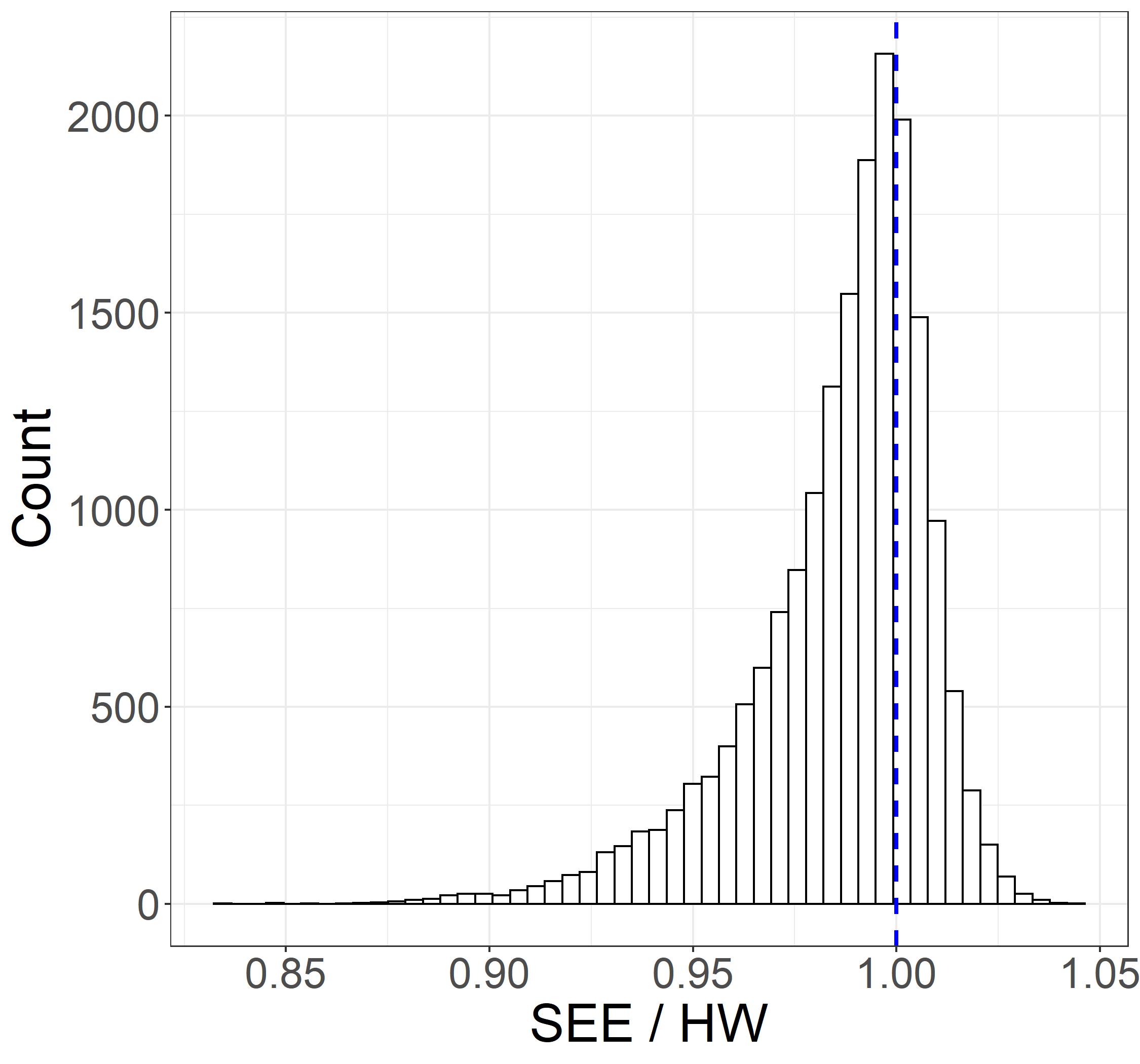
(a)

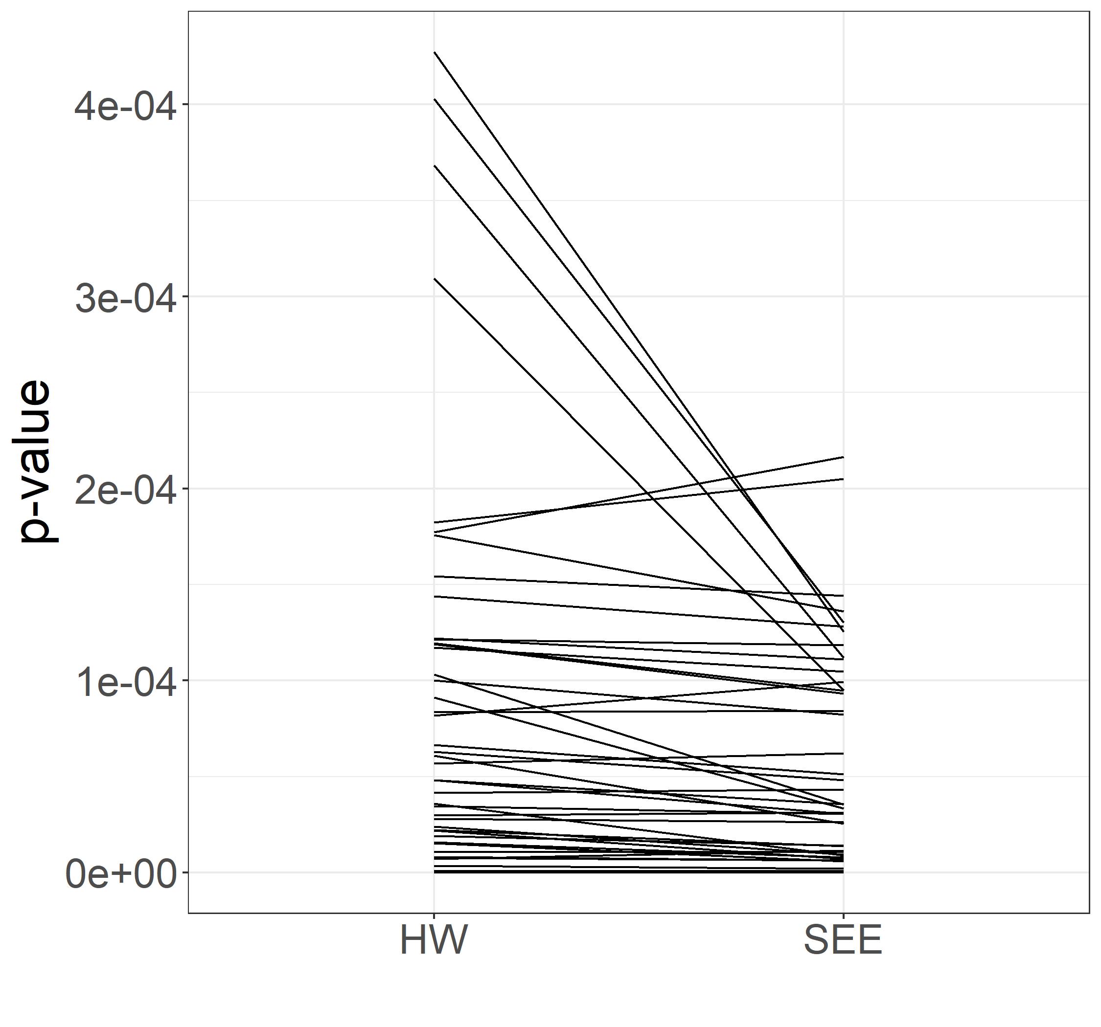
(b)

Figure 1: (a) Ratio of estimated SEs computed using $\hat{\Sigma}$ and $\hat{\Sigma}^{*}$, for the ATT of each gene in the METSIM data analysis. Vertical blue line at ratio value one denotes equality of the two SEs. (b) P-values (unadjusted) for both methods of SE estimation, for each of the top 50 genes as ranked by either method (54 genes depicted in total).

5 Discussion

In the context of variance estimation for the ATT estimator when using IPW, assuming the weights are known can result in either a conservative or an anti-conservative variance estimate. This finding is contrary to the well known result regarding variance estimation for the ATE, namely that assuming the weights are known results in conservative variance estimates. Four simple examples are provided demonstrating that standard error estimates may be substantially larger or smaller depending on whether the weights are treated as known or estimated. Analysis of the METSIM data demonstrated how the different variance estimates can affect the ranking of genes and raw p-values.

The variance estimator using stacked estimating equations is consistent, has a closed-form, and can be easily computed using the geex package in R or the CAUSALTRT procedure in SAS. R code for the asymptotic calculations in Section 2.3 is provided in Appendix C, along with a workflow for analyzing a simulated data set. The bootstrap is another approach to estimating the variance of the IPW ATT estimator (Imbens,, 2004; Abdia et al.,, 2017; Jawid and Khadjavi,, 2019; Were et al.,, 2017), but the bootstrap estimator does not have a closed-form and can be computationally intensive.

Appendix A IPW ATT Estimator Asymptotic Variance

Using block notation, the components of $V(\xi)$ may be expressed as

$$\mathbb{A}(\xi) =-E\left(\begin{array}[]{cc|cc}\partial\psi_{\alpha_{0}}/\partial\alpha_{0}&\partial\psi_{\alpha_{0}}/\partial\alpha_{1}&\partial\psi_{\alpha_{0}}/\partial\mu_{1}&\partial\psi_{\alpha_{0}}/\partial\mu_{0}\\ \partial\psi_{\alpha_{1}}/\partial\alpha_{0}&\partial\psi_{\alpha_{1}}/\partial\alpha_{1}&\partial\psi_{\alpha_{1}}/\partial\mu_{1}&\partial\psi_{\alpha_{1}}/\partial\mu_{0}\\ \hline\cr\partial\psi_{1}/\partial\alpha_{0}&\partial\psi_{1}/\partial\alpha_{1}&\partial\psi_{1}/\partial\mu_{1}&\partial\psi_{1}/\partial\mu_{0}\\ \partial\psi_{0}/\partial\alpha_{0}&\partial\psi_{0}/\partial\alpha_{1}&\partial\psi_{0}/\partial\mu_{1}&\partial\psi_{0}/\partial\mu_{0}\\ \end{array}\right)=\left(\begin{array}[]{cc}a_{11}&0_{(J+1)\times 2}\\ a_{21}&p_{1}I_{2}\end{array}\right)$$

$$\mathbb{B}(\xi) =E\left(\begin{array}[]{cc|cc}\psi_{\alpha_{0}}^{2}&\psi_{\alpha_{0}}\psi_{\alpha_{1}}&\psi_{\alpha_{0}}\psi_{1}&\psi_{\alpha_{0}}\psi_{0}\\ \psi_{\alpha_{1}}\psi_{\alpha_{0}}&\psi_{\alpha_{1}}^{2}&\psi_{\alpha_{1}}\psi_{1}&\psi_{\alpha_{1}}\psi_{0}\\ \hline\cr\psi_{1}\psi_{\alpha_{0}}&\psi_{1}\psi_{\alpha_{1}}&\psi_{1}^{2}&\psi_{1}\psi_{0}\\ \psi_{0}\psi_{\alpha_{0}}&\psi_{0}\psi_{\alpha_{1}}&\psi_{0}\psi_{1}&\psi_{0}^{2}\end{array}\right)=\left(\begin{array}[]{cc}b_{11}&b_{21}^{T}\\ b_{21}&b_{22}\end{array}\right)$$

where $\psi_{\alpha_{0}},\psi_{\alpha_{1}}$ correspond to the score functions for the intercept and the $J$ covariates, respectively, from the logistic regression model (1), and in general $0_{m\times n}$ denotes an $m\times n$ zero matrix, $0_{m}$ denotes a column vector of $m$ zeros, and $I_{m}$ denotes the $m\times m$ identity matrix.

Next note

$$\mathbb{A}(\xi)^{-1}=\left(\begin{array}[]{cc}a_{11}^{-1}&0_{(J+1)\times 2}\\ -p_{1}^{-1}a_{21}a_{11}^{-1}&p_{1}^{-1}I_{2}\end{array}\right)$$

and $a_{11}=b_{11}$ (Lemma 7.3.11, Casella and Berger,, 2002), implying

$$V(\xi) =\left(\begin{array}[]{cc}a_{11}^{-1}&0_{(J+1)\times 2}\\ -p_{1}^{-1}a_{21}a_{11}^{-1}&p_{1}^{-1}I_{2}\end{array}\right)\left(\begin{array}[]{cc}b_{11}&b_{21}^{T}\\ b_{21}&b_{22}\end{array}\right)\left(\begin{array}[]{cc}a_{11}^{-1}&-p_{1}^{-1}a_{11}^{-1}a_{21}^{T}\\ 0_{(J+1)x2}&p_{1}^{-1}I_{2}\end{array}\right)$$

$$=\left(\begin{array}[]{cc}a_{11}^{-1}&p_{1}^{-1}a_{11}^{-1}(-a_{21}+b_{21})^{T}\\ p_{1}^{-1}(-a_{21}+b_{21})a_{11}^{-1}&p_{1}^{-2}\{(a_{21}-b_{21})a_{11}^{-1}(a_{21}-b_{21})^{T}-b_{21}a_{11}^{-1}b_{21}^{T}+b_{22}\}\\ \end{array}\right)$$

By the Delta method, $\Sigma=\nabla g(\xi)^{T}V(\xi)\nabla g(\xi)$ where $\nabla g(\xi)^{T}=(0,0_{J}^{T},1,-1)$. Let $c$ be the $2\times 2$ matrix $c=(a_{21}-b_{21})a_{11}^{-1}(a_{21}-b_{21})^{T}-b_{21}a_{11}^{-1}b_{21}^{T}$, with elements $c_{11},c_{12},c_{21},c_{22}$. Then

$$\Sigma =\nabla g(\xi)^{T}\left(\begin{array}[]{cc}a_{11}^{-1}&p_{1}^{-1}a_{11}^{-1}(-a_{21}+b_{21})^{T}\\ p_{1}^{-1}(-a_{21}+b_{21})a_{11}^{-1}&p_{1}^{-2}(c+b_{22})\\ \end{array}\right)\nabla g(\xi)$$

$$=p_{1}^{-2}\left[E\{A_{i}(Y_{i}^{1}-\mu_{1})^{2}\}+E\{(Y_{i}^{0}-\mu_{0})^{2}h(L_{i};\alpha)e(L_{i};\alpha)\}+c_{11}+c_{22}-c_{12}-c_{21}\right]$$

$$=\Sigma^{*}+p_{1}^{-2}(c_{11}+c_{22}-2c_{12})$$

where the last equality follows from (5) and $c_{12}=c_{21}$ because $V(\xi)$ is symmetric.

Next note

$$a_{21} =\left(\begin{array}[]{cc}0&0_{J}^{T}\\ -E\{(1-A_{i})(Y_{i}-\mu_{0})h(L_{i};\alpha)\}&-E\{(1-A_{i})(Y_{i}-\mu_{0})h(L_{i};\alpha)L_{i}^{T}\}\end{array}\right)$$

$$b_{21} =\left(\begin{array}[]{cc}E\{A_{i}(Y_{i}-\mu_{1})(1-e(L_{i};\alpha))\}&E\{A_{i}(Y_{i}-\mu_{1})(1-e(L_{i};\alpha))L_{i}^{T}\}\\ -E\{(1-A_{i})(Y_{i}-\mu_{0})h(L_{i};\alpha)e(L_{i};\alpha)\}&-E\{(1-A_{i})(Y_{i}-\mu_{0})h(L_{i};\alpha)e(L_{i};\alpha)L_{i}^{T}\}\end{array}\right)$$

where $e(L_{i};\alpha)$ and $h(L_{i};\alpha)$ are as defined in the main text. It follows that

$$(a_{21}-b_{21})a_{11}^{-1} =\left(\begin{array}[]{c}-E[A_{i}(Y_{i}-\mu_{1})\{1-e(L_{i};\alpha)\}(1,L_{i}^{T})]\\ -E\{(1-A_{i})(Y_{i}-\mu_{0})e(L_{i};\alpha)(1,L_{i}^{T})\}\end{array}\right)a_{11}^{-1}$$

Let $m_{1}=A_{i}(Y_{i}-\mu_{1})\{1-e(L_{i};\alpha)\}$, $m_{0}=(1-A_{i})(Y_{i}-\mu_{0})e(L_{i};\alpha)$, and $X_{i}=(1,L_{i}^{T})$. Then

$$(a_{21}-b_{21})a_{11}^{-1}(a_{21}-b_{21})^{T} =\left(\begin{array}[]{c}-E(m_{1}X_{i})\\ -E(m_{0}X_{i})\end{array}\right)a_{11}^{-1}\left(\begin{array}[]{cc}-E(m_{1}X_{i}^{T})&-E(m_{0}X_{i}^{T})\\ \end{array}\right)$$

$$=\left(\begin{array}[]{cc}E(m_{1}X_{i})a_{11}^{-1}E(m_{1}X_{i}^{T})&E(m_{1}X_{i})a_{11}^{-1}E(m_{0}X_{i}^{T})\\ E(m_{0}X_{i})a_{11}^{-1}E(m_{1}X_{i}^{T})&E(m_{0}X_{i})a_{11}^{-1}E(m_{0}X_{i}^{T})\end{array}\right)$$

and

$$b_{21}a_{11}^{-1}b_{21}^{T} =\left(\begin{array}[]{c}E(m_{1}X_{i})\\ -E\{m_{0}h(L_{i};\alpha)X_{i}\}\end{array}\right)a_{11}^{-1}\left(\begin{array}[]{cc}E(m_{1}X_{i}^{T})&-E\{m_{0}h(L_{i};\alpha)X_{i}^{T}\}\end{array}\right)$$

$$=\left(\begin{array}[]{cc}E(m_{1}X_{i})a_{11}^{-1}E(m_{1}X_{i}^{T})&-E(m_{1}X_{i})a_{11}^{-1}E\{m_{0}h(L_{i};\alpha)X_{i}^{T}\}\\ -E\{m_{0}h(L_{i};\alpha)X_{i}\}a_{11}^{-1}E(m_{1}X_{i}^{T})&E\{m_{0}h(L_{i};\alpha)X_{i}\}a_{11}^{-1}E\{m_{0}h(L_{i};\alpha)X_{i}^{T}\}\end{array}\right)$$

implying

$$c =\left(\begin{array}[]{cc}0&E(m_{1}X_{i})a_{11}^{-1}E[m_{0}\{1+h(L_{i};\alpha)\}X_{i}^{T}]\\ E[m_{0}\{1+h(L_{i};\alpha)\}X_{i}]a_{11}^{-1}E(m_{1}X_{i}^{T})&E(m_{0}X_{i})a_{11}^{-1}E(m_{0}X_{i}^{T})-\\ &\qquad E\{m_{0}h(L_{i};\alpha)X_{i}\}a_{11}^{-1}E\{m_{0}h(L_{i};\alpha)X_{i}^{T}\}\end{array}\right)$$

Assume the propensity score model (1) and conditional exchangeability, the expectations above can be expressed

$$E(m_{1}X_{i}) =E[A_{i}(Y_{i}-\mu_{1})\{1-e(L_{i};\alpha)\}(1,L_{i}^{T})]$$

$$=E[A_{i}(Y_{i}^{1}-\mu_{1})\{1-P(A_{i}=1|L_{i})\}(1,L_{i}^{T})]$$

$$=E_{L}\left[E_{Y^{1}|L}(Y_{i}^{1}-\mu_{1})\ P(A_{i}=1|L_{i})\{1-P(A_{i}=1|L_{i})\}\ (1,L_{i}^{T})\right]$$

and similarly $E(m_{0}X_{i})=E_{L}\left[E_{Y^{0}|L}(Y_{i}^{0}-\mu_{0})\ P(A_{i}=1|L_{i})\{1-P(A_{i}=1|L_{i})\}(1,L_{i}^{T})\right]$ and
$E\{m_{0}h(L_{i};\alpha)X_{i}\}=E_{L}\{E_{Y^{0}|L}(Y_{i}^{0}-\mu_{0})\ P(A_{i}=1|L_{i})^{2}(1,L_{i}^{T})\}$, which implies
$E\left[m_{0}\{1+h(L_{i};\alpha)\}X_{i}\right]=E_{L}\{E_{Y^{0}|L}(Y_{i}^{0}-\mu_{0})\ P(A_{i}=1|L_{i})(1,L_{i}^{T})\}$.

Likewise, $a_{11}^{-1}=b_{11}^{-1}$ can be written

$$a_{11}^{-1} =\frac{1}{det(a_{11})}\left(\begin{array}[]{cc}E(\psi_{\alpha_{1}}\psi_{\alpha_{1}}^{T})&-E(\psi_{\alpha_{0}}\psi_{\alpha_{1}})^{T}\\ -E(\psi_{\alpha_{0}}\psi_{\alpha_{1}})&E(\psi_{\alpha_{0}}^{2})\end{array}\right)$$

where $det(a_{11})=E(\psi_{\alpha_{0}}^{2})E(\psi_{\alpha_{1}}\psi_{\alpha_{1}}^{T})-E(\psi_{\alpha_{0}}\psi_{\alpha_{1}})E(\psi_{\alpha_{0}}\psi_{\alpha_{1}})^{T}$. The elements of this matrix can be expressed

$$E(\psi_{\alpha_{0}}^{2}) =E\{A_{i}-2A_{i}P(A_{i}=1|L_{i})+P(A_{i}=1|L_{i})^{2}\}$$

$$=E_{L}[P(A_{i}=1|L_{i})\{1-P(A_{i}=1|L_{i})\}]$$

with similar derivations for $E(\psi_{\alpha_{0}}\psi_{\alpha_{1}})=E_{L}[P(A_{i}=1|L_{i})\{1-P(A_{i}=1|L_{i})\}L_{i}]$ and $E(\psi_{\alpha_{1}}\psi_{\alpha_{1}}^{T})=E_{L}[P(A_{i}=1|L_{i})\{1-P(A_{i}=1|L_{i})\}L_{i}L_{i}^{T}]$.

Using the results above, explicit values for each element of the $c$ matrix can be calculated for given distributions of $L$, $A|L$, $Y^{0}|L$, and $Y^{1}|L$. This is demonstrated in Section 2.3 for four example scenarios. The R code used for these calculations is included in Appendix C.

Appendix B Expected Value of ATT Weights

The expected value of the weights proposed by Sato and Matsuyama, (2003) equals

$$E[W_{i}^{ATT}] =E_{A,L}\left[A_{i}+(1-A_{i})\frac{P(A_{i}=1|L_{i})}{P(A_{i}=0|L_{i})}\right]$$

$$=p_{1}+E_{L}\left[E_{A|L}(1-A_{i})\frac{P(A_{i}=1|L_{i})}{P(A_{i}=0|L_{i})}\right]$$

$$=p_{1}+E_{L}\left[P(A_{i}=1|L_{i})\right]=2p_{1}$$

Appendix C Example R Code

The code below was written for the R environment in R version 3.6.3 (R Core Team,, 2020).

C.1 Asymptotic Calculations

First set the values of the parameters from scenario (i) in the main text.

EL <- 0.5 ; a0 <- -1 ; a1 <- -2

ba <- -1 ; bL <- -1.5 ; baL <- 1.5 ; sdY <- 0.5

From these defined values we can solve for the other needed quantities.

EA_L1 <- exp(a0 + a1) / (1 + exp(a0 + a1))

EA_L0 <- exp(a0) / (1 + exp(a0))

EY1_L1 <- ba + bL + baL #no intercept term

EY1_L0 <- ba

EY0_L1 <- bL

EY0_L0 <- 0

VarY0_L <- sdY^2

VarY1_L <- sdY^2

EA <- EA_L0*(1-EL) + EA_L1*(EL)

EL_A1 <- (1/EA) * EA_L1 * EL

mu0 <- bL * EL_A1

mu1 <- ba + bL*EL_A1 + baL*EL_A1

ATT <- mu1-mu0

These values can be plugged in to calculate the elements of the $a_{21},\ b_{21},$ and $a_{11}^{-1}$ matrices.

## Calculate required expectations for (a21 - b21),

##  b21, and a11^{-1} matrices

a21_b21.1 <- (EY1_L0 - mu1)*EA_L0*(1-EA_L0)*(1-EL) +

                (EY1_L1 - mu1)*EA_L1*(1-EA_L1)*EL

a21_b21.2 <- (EY0_L0 - mu0)*EA_L0*(1-EA_L0)*(1-EL) +

                (EY0_L1 - mu0)*EA_L1*(1-EA_L1)*EL

a21_b21.3 <- (EY1_L0 - mu1)*EA_L0*(1-EA_L0)*0*(1-EL) +

                (EY1_L1 - mu1)*EA_L1*(1-EA_L1)*1*EL

a21_b21.4 <- (EY0_L0 - mu0)*EA_L0*(1-EA_L0)*0*(1-EL) +

                (EY0_L1 - mu0)*EA_L1*(1-EA_L1)*1*EL

a21_b21 <- matrix(c(-a21_b21.1, -a21_b21.2, -a21_b21.3, -a21_b21.4),

                    nrow=2, ncol=2)

b21.2 <- (EY0_L0 - mu0)*(EA_L0^2)*(1-EL) +

              (EY0_L1 - mu0)*(EA_L1^2)*EL

b21.4 <- (EY0_L0 - mu0)*(EA_L0^2)*0*(1-EL) +

              (EY0_L1 - mu0)*(EA_L1^2)*1*EL

b21 <- matrix(c(a21_b21.1, -b21.2, a21_b21.3, -b21.4),

                nrow=2, ncol=2)

a11_1 <- EA_L0*(1-EA_L0)*(1-EL) + EA_L1*(1-EA_L1)*EL

a11_2 <- EA_L0*(1-EA_L0)*0*(1-EL) + EA_L1*(1-EA_L1)*1*EL

a11_3 <- EA_L0*(1-EA_L0)*(0^2)*(1-EL) + EA_L1*(1-EA_L1)*(1^2)*EL

a11 <- matrix(c(a11_1, a11_2, a11_2, a11_3),

                nrow=2, ncol=2)

a11_inv <- solve(a11)

What remains is simply using matrix algebra to calculate values of the constant and $\Sigma^{*}$.

## Calculate constant

c <- a21_b21 %*% a11_inv %*% t(a21_b21) - b21 %*% a11_inv %*% t(b21)

c_scaled <- (1/EA^2)*c  # (1/P(A=1)^2) * c

gg <- cbind(c(1, -1))

constant <- t(gg) %*% c_scaled %*% gg

## Calculate Sigma* and Sigma

EY0_mu02_L0 <- (VarY0_L + EY0_L0^2) - 2*mu0*EY0_L0 + mu0^2

EY0_mu02_L1 <- (VarY0_L + EY0_L1^2) - 2*mu0*EY0_L1 + mu0^2

EY1_mu12_L0 <- (VarY1_L + EY1_L0^2) - 2*mu1*EY1_L0 + mu1^2

EY1_mu12_L1 <- (VarY1_L + EY1_L1^2) - 2*mu1*EY1_L1 + mu1^2

b22_1 <- (EA_L0*EY1_mu12_L0)*(1-EL) + (EA_L1*EY1_mu12_L1)*EL

b22_2 <- ((EA_L0^2/(1-EA_L0))*EY0_mu02_L0)*(1-EL) +

            ((EA_L1^2/(1-EA_L1))*EY0_mu02_L1)*EL

Sig_star <- (b22_1 + b22_2)/(EA^2)

Sig <- Sig_star + constant

df <- data.frame(cbind(ATT, constant, Sig_star, Sig))

colnames(df) <- c("ATT", "Constant", "Sigma^*", "Sigma")

print(df)

##          ATT Constant  Sigma^*    Sigma
## 1 -0.7751385 1.635956 2.263171 3.899128

These results align with those presented in Table 2.

C.2 Simulated Data Analysis

Using the population parameters defined above, we can simulate an example data set of 1000 individuals. After generating $L,\ A,$ and $Y$, the ATT weights are computed as in the main text.

set.seed(42)

n <- 1000

L <- rbinom(n, 1, prob = EL)

lp <- exp(a0 + a1*L)

A <- rbinom(n, size = 1, prob = lp/(1+lp))

Y <- rnorm(n, mean = ba*A + bL*L + baL*A*L, sd = sdY)

psmod <- glm(A ~ L, family = binomial(link = "logit"))

wt.att <- ifelse(A == 0, exp(psmod$linear.predictors), 1)

dat <- data.frame(cbind(L, A, Y, wt.att))

The following are helper functions defined for use within the geex function m_estimate, which will allow us to compute the standard errors for the stacked estimating equations (SEE) and robust (Huber-White) variance estimators.

estfun <- function(data, model){

  L <- model.matrix(model, data=data)

  A <- model.response(model.frame(model, data=data))

  Y <- data$Y

  function(theta){

    p  <- length(theta)

    p1 <- length(coef(model))

    lp  <- L %*% theta[1:p1]

    rho <- plogis(lp)

    IPW <- ifelse(A == 1, 1, exp(lp))

    score_eqns <- apply(L, 2, function(x) sum((A - rho) * x))

    ce1 <- IPW*(A==1)*(Y - theta[p-1])

    ce0 <- IPW*(A==0)*(Y - theta[p])

    c(score_eqns,

      ce1,

      ce0)

  }

}

estfun_nolr <- function(data){

  A <- data$A

  Y <- data$Y

  IPW <- data$wt.att

  function(theta){

    ce1 <- IPW*(A==1)*(Y - theta[1])

    ce0 <- IPW*(A==0)*(Y - theta[2])

    c(ce1,

      ce0)

  }

}

Fitting the weighted linear regression model yields the estimated counterfactual means, from which we can compute the estimated ATT.

fit <- geeglm(Y ~ A, data = dat, std.err = ’san.se’,

                weights = wt.att, id=1:nrow(dat),

                corstr="independence")

mu1_hat <- mean(fit$fitted.values[fit$dat$A==1])

mu0_hat <- mean(fit$fitted.values[fit$dat$A==0])

ATT_Est <- fit$coefficients[2]  # = mu1_hat - mu0_hat

Finally, the geex package is used to estimate the SEs of the estimated ATT using both the SEE and the Huber-White estimators. The Huber-White SEs are also computed with the geeglm function to check the output from m_estimate.

## Accounting for weight estimation

results <- m_estimate(

              estFUN = estfun,

              data  = dat,

              roots = c(coef(psmod), mu1_hat, mu0_hat),

              compute_roots = FALSE,

              outer_args = list(model = psmod))

## b22 + [1/P(A=1)^2]c

vcov_sEE <- vcov(results)[3:4, 3:4]

## Assuming weights are known

results_nolr <- m_estimate(

                    estFUN = estfun_nolr,

                    data  = dat,

                    roots = c(mu1_hat, mu0_hat),

                    compute_roots = FALSE)

## b22

vcov_GEE <- vcov(results_nolr)

## Robust (Huber-White) Variance from geeglm for comparison

vcov_geeglm <- (summary(fit)$coefficients[2,2])^2

Sig_est <- t(gg) %*% vcov_sEE %*% gg

Sig_star_est <- t(gg) %*% vcov_GEE %*% gg

df <- data.frame(cbind(ATT_Est, sqrt(Sig_est),

                       sqrt(Sig_star_est), sqrt(vcov_geeglm)))

colnames(df) <- c("Est ATT", "Est SEE SE",

                  "Est HW SE (geex)", "Est HW SE (geeglm)")

print(df)

##      Est ATT Est SEE SE Est HW SE (geex) Est HW SE (geeglm)
## A -0.7543794 0.05830972       0.04407246         0.04407246

As you can see, the SE estimates from geeglm and from geex when weights are assumed known are the same. All estimates resemble the results presented in Table 3, but do not match exactly since this code was only run on one example data set and the Table 3 results are averaged over 1000 data sets.

Note that when performing the analysis for a large number of simulated data sets or, e.g., a large genomics data set such as METSIM with hundreds or thousands of individuals and outcomes, there is a practical need to run the code for analyzing these data sets simultaneously on a compute cluster.

References

- Abdia et al., (2017) Abdia, Y., Kulasekera, K. B., Datta, S., Boakye, M., and Kong, M. (2017). Propensity scores based methods for estimating average treatment effect and average treatment effect among treated: A comparative study. Biometrical Journal, 59(5):967–985.
- Addai et al., (2014) Addai, K. N., Owusu, V., and Addai, K. N. and Owusu, V. (2014). Effects of Farmer – Based- Organization on the Technical efficiency of Maize Farmers across Various Agro - Ecological Zones of Ghana. Journal of Economics and Development Studies, 3(1):149–172.
- Apel and Sweeten, (2010) Apel, R. J. and Sweeten, G. (2010). Propensity score matching in criminology and criminal justice. In Piquero, A. R. and Weisburd, D., editors, Handbook of Quantitative Criminology, pages 543–562. Springer, New York, NY.
- Austin, (2011) Austin, P. C. (2011). An introduction to propensity score methods for reducing the effects of confounding in observational studies. Multivariate Behavioral Research, 46(3):399–424.
- Bodory et al., (2018) Bodory, H., Camponovo, L., Huber, M., and Lechner, M. (2018). The Finite Sample Performance of Inference Methods for Propensity Score Matching and Weighting Estimators. Journal of Business and Economic Statistics, 15:183–200.
- Boulay et al., (2014) Boulay, M., Lynch, M., and Koenker, H. (2014). Comparing two approaches for estimating the causal effect of behaviour-change communication messages promoting insecticide-treated bed nets: An analysis of the 2010 Zambia malaria indicator survey. Malaria Journal, 13(1):1–8.
- Brookhart et al., (2013) Brookhart, M. A., Wyss, R., Layton, J. B., and Stürmer, T. (2013). Propensity Score Methods for Confounding Control in Nonexperimental Research. Circulation: Cardiovascular Quality and Outcomes, 6(5):604–611.
- Casella and Berger, (2002) Casella, G. and Berger, R. L. (2002). Statistical Inference, Second Edition. Duxbury Pacific Grove, CA.
- Civelek et al., (2017) Civelek, M., Wu, Y., Pan, C., Raulerson, C. K., Ko, A., He, A., Tilford, C., Saleem, N. K., Stančáková, A., Scott, L. J., et al. (2017). Genetic Regulation of Adipose Gene Expression and Cardio-Metabolic Traits. American Journal of Human Genetics, 100(3):428–443.
- Gross and Rosenheim, (2011) Gross, K. and Rosenheim, J. A. (2011). Quantifying secondary pest outbreaks in cotton and their monetary cost with causal- inference statistics. Ecological Applications, 21(7):2770–2780.
- Heckman and Vytlacil, (2001) Heckman, J. J. and Vytlacil, E. (2001). Policy-Relevant Treatment Effects. The American Economic Review, 91:107–111.
- Hernán and Robins, (2020) Hernán, M. and Robins, J. (2020). Causal Inference: What If. Chapman & Hall/CRC, Boca Raton.
- Imbens, (2004) Imbens, G. W. (2004). Nonparametric estimation of average treatment effects under exogeneity: A review. Review of Economics and Statistics, 86(1):4–29.
- Jawid and Khadjavi, (2019) Jawid, A. and Khadjavi, M. (2019). Adaptation to climate change in Afghanistan: Evidence on the impact of external interventions. Economic Analysis and Policy, 64:64–82.
- Laakso et al., (2017) Laakso, M., Kuusisto, J., Stančáková, A., Kuulasmaa, T., Pajukanta, P., Lusis, A. J., Collins, F. S., Mohlke, K. L., and Boehnke, M. (2017). The Metabolic Syndrome in Men study: A resource for studies of metabolic & cardiovascular diseases. Journal of Lipid Research, 58(3):481–493.
- Lunceford and Davidian, (2004) Lunceford, J. K. and Davidian, M. (2004). Stratification and weighting via the propensity score in estimation of causal treatment effects: A comparative study. Statistics in Medicine, 23(19):2937–2960.
- Marcus, (2014) Marcus, J. (2014). Does Job Loss Make You Smoke and Gain Weight? Economica, 81(324):626–648.
- Moodie et al., (2018) Moodie, E. E. M., Saarela, O., and Stephens, D. A. (2018). A doubly robust weighting estimator of the average treatment effect on the treated. Stat, 7(1):e205.
- Morris, (2016) Morris, R. G. (2016). Exploring the Effect of Exposure to Short-Term Solitary Confinement Among Violent Prison Inmates. Journal of Quantitative Criminology, 32(1):1–22.
- Nduka et al., (2016) Nduka, C. U., Stranges, S., Bloomfield, G. S., Kimani, P. K., Achinge, G., Malu, A. O., and Uthman, O. A. (2016). A plausible causal link between antiretroviral therapy and increased blood pressure in a sub-Saharan African setting: A propensity score-matched analysis. International Journal of Cardiology, 220:400–407.
- Pirracchio et al., (2016) Pirracchio, R., Carone, M., Rigon, M. R., Caruana, E., Mebazaa, A., and Chevret, S. (2016). Propensity score estimators for the average treatment effect and the average treatment effect on the treated may yield very different estimates. Statistical Methods in Medical Research, 25(5):1938–1954.
- R Core Team, (2020) R Core Team (2020). R: A Language and Environment for Statistical Computing. R Foundation for Statistical Computing, Vienna, Austria.
- Ramsey et al., (2019) Ramsey, D. S., Forsyth, D. M., Wright, E., McKay, M., and Westbrooke, I. (2019). Using propensity scores for causal inference in ecology: Options, considerations, and a case study. Methods in Ecology and Evolution, 10(3):320–331.
- Rawat et al., (2010) Rawat, R., Kadiyala, S., and McNamara, P. E. (2010). The impact of food assistance on weight gain and disease progression among HIV-infected individuals accessing AIDS care and treatment services in Uganda. BMC Public Health, 10:316.
- Reifeis et al., (2020) Reifeis, S. A., Hudgens, M. G., Civelek, M., Mohlke, K. L., and Love, M. I. (2020). Assessing exposure effects on gene expression. Genetic Epidemiology, 44(6):601–610.
- Rubin, (1980) Rubin, D. B. (1980). Randomization analysis of experimental data: The fisher randomization test comment. Journal of the American Statistical Association, 75(371):591–593.
- SAS Institute Inc., (2018) SAS Institute Inc. (2018). User’s Guide The CAUSALTRT Procedure. In SAS/STAT 15.1 User’s Guide, chapter 36, pages 2365–2423. SAS Institute Inc., Cary, NC.
- Sato and Matsuyama, (2003) Sato, T. and Matsuyama, Y. (2003). Marginal structural models as a tool for standardization. Epidemiology, 14(6):680–686.
- Saul and Hudgens, (2020) Saul, B. C. and Hudgens, M. G. (2020). The Calculus of M-Estimation in R with geex. Journal of Statistical Software, 92(2):1–15.
- Stefanski and Boos, (2002) Stefanski, L. and Boos, D. (2002). The Calculus of M-Estimation. The American Statistician, 56(1):29–38.
- Tamini, (2011) Tamini, L. D. (2011). A nonparametric analysis of the impact of agri-environmental advisory activities on best management practice adoption: A case study of Québec. Ecological Economics, 70(7):1363–1374.
- Taylor et al., (2013) Taylor, A., Westveld, A. H., Szkudlinska, M., Guruguri, P., Annabi, E., Patwardhan, A., Price, T. J., and Yassine, H. N. (2013). The use of metformin is associated with decreased lumbar radiculopathy pain. Journal of Pain Research, 6:755–763.
- van der Wal and Geskus, (2011) van der Wal, W. M. and Geskus, R. B. (2011). ipw: An R package for inverse probability weighting. Journal of Statistical Software, 43(13):2–23.
- Were et al., (2017) Were, L. P., Were, E., Wamai, R., Hogan, J., and Galarraga, O. (2017). The association of health insurance with institutional delivery and access to skilled birth attendants: Evidence from the Kenya demographic and health survey 2008-09. BMC Health Services Research, 17(1):1–10.
- Widdowson et al., (2016) Widdowson, A. O., Siennick, S. E., and Hay, C. (2016). The Implications of Arrest for College Enrollment: an Analysis of Long-Term Effects and Mediating Mechanisms. Criminology, 54(4):621–652.