Quantum transport in a combined kicked rotor and quantum walk system

Abstract

We present a theoretical and numerical study of the competition between two opposite interference effects, namely interference-induced ballistic transport on one hand, and strong (Anderson) localization on the other. While the former effect allows for resistance free transport, the latter brings the transport to a complete halt. As a model system, we consider the quantum kicked rotor, where strong localization is observed in the discrete momentum coordinate. In this model, we introduce the ballistic transport in the form of a Hadamard quantum walk in that momentum coordinate. The two transport mechanisms are combined by alternating the corresponding Floquet operators.

Extending the corresponding calculation for the kicked rotor, we estimate the classical diffusion coefficient for the combined dynamics. Another argument, based on the introduction of an effective Heisenberg time should then allow to estimate the localization time and the localization length. While this is known to work reasonably well in the kicked rotor case, we find that it fails in our case. While the combined dynamics still shows localization, it takes place at much larger times and shows much larger localization lengths than predicted.

Finally, we combine the kicked rotor with other types of quantum walks, namely diffusive and localizing quantum walks. In the diffusive case, the localizing dynamics of the kicked rotor is completely canceled and we get pure diffusion. In the case of the localizing quantum walk, the combined system remains localized, but with a larger localization length.

1 Introduction

Interference effects at the border between classical and quantum transport have been of particular interest as they are capable of changing the transport properties of a system completely. One classic example is the strong localization (Anderson localization) [1], where the destructive interference between many random paths leads to a complete halt of transport. Modifications of strong localization have been studied in the last couple of years, for instance, the inclusion of nonlinear effects in the Anderson model [2] and weak nonlinearity combined with a static field [3]. The inclusion of such effects weakens the strong localization.

Another, more recent example, is that of quantum (random) walks [4, 5] which were first been proposed in Ref. [6]. There, the interference between several paths may lead to quite the opposite effect, changing the transport from diffusive to ballistic. Applications for this effect can be found in the area of quantum computing and quantum versions of classical Monte Carlo search algorithms [5] (and references therein).

In this paper, we study the competition of two wave phenomena, which, from a quantum transport perspective, lead eventually to opposite results. On the one hand, “strong localization”, which essentially brings quantum transport to a halt, and on the other hand the Hadamard quantum walk (QW) [5], which may turn a classically diffusive process into one of ballistic transport. A convenient arena for this competition is the quantum kicked rotor (KR) [7, 8], which shows strong localization in the discrete momentum coordinate, and where different types of quantum walk can be implemented in a natural way.

Both, the KR and the QW can be realized experimentally on a number of experimental platforms [9, 10, 11, 12]. In addition, recently, it has been shown that the QW dynamics can be realized in a KR system, when the kick period is in resonance with the period of the rotor [13, 14, 15].

In the case of the KR, strong localization is not due to disorder but to quantum chaos. Consequently, one rather speaks about “dynamical localization” [7, 16, 8]. Still, it is possible to map the dynamics on a tight binding model with quasi-random disorder, similar to the one-dimensional Anderson model [17, 18].

A quantum walk (QW) may be considered as the quantum version of a classical random walk [4, 5]. While it can be discrete or continuous in time, we limit ourselves to the discrete case. A classical random walker on a one-dimensional lattice, chooses at each step to move either to the left or to the right. If this choice is random, the corresponding dynamics are diffusive and the variance of the walkers position increase linearly with time. In contrast, the quantum walker chooses between stepping to the left or stepping to the right, depending on the state of a two-level quantum system – the quantum “coin”. By making sure that this coin is always in a superposition state, the quantum walker will perform a superposition of both steps. In this case the variance of the walker position increases quadratically in time, which is known as ballistic motion. If we perform measurements upon the walker, or if there is a general decoherence process, such as measurements of the walkers position, then the quantum walk “collapses” to the classical random walk, and diffusive motion is recovered [19, 20].

In both cases, quantum KR and QW, the dynamics is generated by the repeated application of discrete (Floquet) evolution operators, $F_{\rm kr}$ and $F_{\rm qw}$, respectively. Therefore, we generate the dynamics of the combined system by simply alternating the two Floquet operators. The QW is implemented in the discrete momentum coordinate, since it is there where the dynamical localization of the quantum KR takes place. To vary the relative strength between the two models, we use the kick strength in the KR, which controls the localization length of the dynamics. In addition, we consider different step sizes for the QW.

Additional control of the dynamics of the combined system is achieved by choosing the operations on the quantum coin (a two level system which controls the direction of the quantum walker) in different ways: (i) the so called “Hadamard” QW, where the coin operation is a Hadamard gate, and the resulting QW is ballistic; (ii) coin operations which are random in space and time, so that the resulting QW is diffusive; (iii) coin operations which are random in space only, so that the resulting QW is localized. Mainly, we focus on the standard Hadamard QW case, however, in a final section, we also analyse the case where the QW part is either diffusive or localized.

The paper is organized as follows. After the introduction (Sec. 1), we review the localization properties of the quantum KR in Sec. 2, and discuss the discrete time quantum walk (QW) in Sec. 3. Sec. 4 contains a detailed analysis (numerical and analytical) of the localization properties of the combined system. We end the paper in Sec. 5 with our conclusions.

2 Kicked rotor

Here, we review the diffusion and localization properties of the kicked rotor. In Sec. 2.1 we discuss the classical kicked rotor, in Sec. 2.2 the corresponding quantum system. The classical kicked rotor can be reduced to a one-parameter family of dynamical maps, while the quantum kicked rotor has an additional independent parameter which is reminiscent to Planck’s constant.

2.1 Classical kicked rotor

For future reference, and for an unambiguous definition of the variables and parameters to be used throughout this work, we shortly review the dynamical equations which define the kicked rotor. Its dynamics are described in two-dimensional phase space, which consists of the angle variable, $-\pi\leq\theta<\pi$, and the angular momentum variable, $L\in\mathbb{R}$. The Hamiltonian reads

$$H(L,\theta)=\frac{L^{2}}{2I}+K\;\cos\theta\;\sum_{n\in\mathbb{Z}}\delta(t_{\rm ph}-n\,T)\;,$$ (1)

where $K$ is the kick strength, $T$ the kick period and $t_{\rm ph}$ the time in physical units. In the absence of kicks, $L$ is constant and $\theta(t)=\theta(0)+Lt_{\rm ph}/I$. That means that between two kicks, $\theta$ changes as follows:

$$\theta^{\prime}=\theta+\frac{L\,t_{\rm ph}}{I}+2\pi m\;,$$ (2)

where $m\in\mathbb{Z}$ is chosen such that $\theta$ remains inside the interval $[-\pi,\pi)$. The kick by contrast is instantaneous and leaves $\theta$ unchanged. However, for $L$ we find

$$L^{\prime}=L+K\;\sin\theta\;.$$ (3)

Putting both processes together (starting with the kick), we find

$$\begin{split}L_{t+1}&=L_{t}+K\;\sin\theta\;,\\ \theta_{t+1}&=\theta_{t}+\frac{T}{I}\;L_{t+1}=\theta_{t}+\frac{T}{I}\;\big{(}\,L_{t}+K\;\sin\theta\,\big{)}\;,\end{split}$$ (4)

where the integer $t$ measures time in units of the kick period $T$. Multiplying the first equation with $T/I$, and redefining $p_{t}=T\,L_{t}/I$, we find

$$\begin{split}p_{t+1}&=p_{t}+\kappa\;\sin\theta\;,\\ \theta_{t+1}&=\theta_{t}+p_{t}+\kappa\;\sin\theta\;,\end{split}$$ (5)

where $\kappa=TK/I$. This shows, that the classical kicked rotor is essentially a one-parameter family of dynamical maps, parametrized by $\kappa$, see e.g. [21].

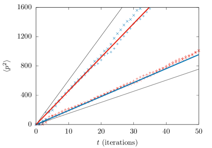
Figure 1: Second moment of the momentum as a function of time, showing classical diffusion, for $\kappa=5.5$ (red points) and $11.0$ (blue points). The solid black lines show the simple classical expectation according to Eq. (6), the colored straight lines are obtained from the improved theoretical estimate for the diffusion constant in Eq. (8) – for $\kappa=5.5$ (blue line) and $\kappa=11.0$ (red line). We averaged over $N_{\rm sam}=1000$ trajectories with initial conditions in phase space, chosen from a central square region of size $0.1\times 0.1$ ($+$ symbols) and $1.0\times 1.0$ ($\times$ symbols), respectively.

Diffusion in momentum space

We compute trajectories for the kicked rotor map given in Eq. (5) for $\kappa=5.5$ and $\kappa=11.0$ and plot the average kinetic energy as a function of time (number of iterations). As initial conditions, we choose initial points uniformly in a square region of side lengths $\Delta$ around the center of phase space. A simple argument which assumes statistical independence of subsequent iterations yields:

$$\langle p^{2}_{t+1}\rangle=\frac{\kappa^{2}}{2}\;\langle p^{2}_{t}\rangle\;.$$ (6)

However, in Ref. [16] this estimation has been replaced by the more accurate expression

$$\sigma^{2}_{p}(t)=\langle p_{t}^{2}\rangle-\langle p_{t}\rangle^{2}\approx D_{0}\;t\;,$$ (7)

with the classical diffusion constant (in momentum space) given as

$$D_{0}=\frac{1}{2}\begin{cases}\kappa^{2}\,\big{[}\,1-2\,J_{2}(\kappa)+2\,J_{2}(\kappa)^{2}\,\big{]}&:\kappa\geq 4.5\\ 0.6\;(\kappa-\kappa_{\rm cr})^{3}&:\kappa_{\rm cr}<\kappa<4.5\end{cases}\;.$$ (8)

Here, $\kappa_{\rm cr}\approx 0.9716$ and $J_{2}(x)$ is the Bessel function [22].

In Fig. 1, we illustrate the diffusion in the momentum coordinate of the classical kicked rotor for two different values of $\kappa$. These values, $\kappa=5.5$ ($\kappa=11.0$) are chosen in such a way that the more precise estimation for the diffusion coefficient $D$ is above (below) the simple estimates (solid black lines) from Eq. (6). It can be seen that the numerical data follow the improved expression from Eq. (8) rather accurately.

2.2 Quantum kicked rotor

The Hamiltonian in the quantum case is given by

$$\frac{\hat{L}^{2}}{2I}+K\cos\hat{\theta}\;\sum_{n\in\mathbb{Z}}\delta(t_{\rm ph}-n\,T)\;,\qquad\hat{L}=-\mathrm{i}\,\hbar\,\partial_{\theta}\;.$$ (9)

The time evolution between two kicks is given as

$$U_{\rm free}=\mathrm{e}^{-\mathrm{i}\hat{L}^{2}\,T/(2I\,\hbar)}\quad\text{with}\quad[\hat{L},\hat{\theta}]=\mathrm{i}\,\hbar\;.$$ (10)

Let us rescale the angular momentum operator $\hat{L}$ and introduce a dimensionless effective Planck constant $\hbar_{\rm eff}$. Then we may write

$$\hat{p}=\frac{T}{I}\;\hat{L}\;,\quad\hbar_{\rm eff}=\frac{\hbar\,T}{I}\quad:\quad U_{\rm free}=\mathrm{e}^{-\mathrm{i}\hat{p}^{2}/(2\hbar_{\rm eff})}\;,$$ (11)

with the new commutation relation $[\hat{p},\hat{\theta}]=\mathrm{i}\,\hbar_{\rm eff}$. The kick itself affects the system via another unitary operator, namely

$$U_{\rm kick}=\mathrm{e}^{-\mathrm{i}K\,\cos(\hat{\theta})/\hbar}=\mathrm{e}^{-\mathrm{i}\kappa\,\cos(\hat{\theta})/\hbar_{\rm eff}}\;,$$ (12)

which can be seen by solving the Schrödinger equation in position (i.e. angle) representation (see A), while using the dimensionless kick strength $\kappa$, as defined in Eq. (5).

Momentum representation

The eigenstates of $\hat{p}$ are the periodic plane waves,

$$\varphi_{m}(\theta)=\frac{\mathrm{e}^{\mathrm{i}m\,\theta}}{\sqrt{2\pi}}$$ (13)

such that

$$\hat{p}\;\varphi_{m}(\theta)=-\mathrm{i}\hbar_{\rm eff}\,\partial_{\theta}\;\varphi_{m}(\theta)=\hbar_{\rm eff}\,m\;\varphi_{m}(\theta)$$ (14)

with $m\in\mathbb{Z}$. This allows to write

$$U_{\rm free}=\sum_{m\in\mathbb{Z}}|\varphi_{m}\rangle\;\mathrm{e}^{-\mathrm{i}\hbar_{\rm eff}\,m^{2}/2}\;\langle\varphi_{m}|\;.$$ (15)

In what follows, we use the simpler notation $|m\rangle=|\varphi_{m}\rangle$ for the eigenstates of the momentum operator.

It remains to find the momentum representation of the operator $U_{\rm kick}$. For that purpose, we need to evaluate the following integral:

$$\langle m|U_{\rm kick}\,|n\rangle=\frac{1}{2\pi}\int_{0}^{2\pi}\mathrm{d}\theta\;\mathrm{e}^{\mathrm{i}(n-m)\,\theta}\;\mathrm{e}^{-\mathrm{i}\kappa/\hbar_{\rm eff}\ \cos\theta}\;.$$ (16)

This is achieved with the help of the formula [22],

$$\mathrm{e}^{-\mathrm{i}z\cos\theta}=\sum_{k\in\mathbb{Z}}(-\mathrm{i})^{k}\;J_{k}(z)\;\mathrm{e}^{\mathrm{i}k\theta}\;,$$ (17)

which yields

$$\begin{split}&\langle m|U_{\rm kick}\,|n\rangle=\sum_{k\in\mathbb{Z}}(-\mathrm{i})^{k}\;J_{k}(z)\;\frac{1}{2\pi}\int_{0}^{2\pi}\mathrm{d}\theta\mathrm{e}^{\mathrm{i}(n-m)\,\theta}\;\mathrm{e}^{\mathrm{i}k\theta}\\ &\qquad=\sum_{k\in\mathbb{Z}}(-\mathrm{i})^{k}\;J_{k}(z)\;\delta_{n-m+k}=(-\mathrm{i})^{m-n}\;J_{m-n}(z)\;,\end{split}$$ (18)

where we have set $z=\kappa/\hbar_{\rm eff}$. In our simulations of the quantum kicked rotor, we use the symmetrized version of the Floquet operator [8],

$$F_{\rm kr}=U_{\rm free}^{1/2}\;U_{\rm kick}\;U_{\rm free}^{1/2}\;,$$ (19)

and for the evolution of quantum states $\Psi(t)$, we use

$$\Psi(t+1)=F_{\rm kr}\;\Psi(t)\;,$$ (20)

where the integer $t$ measures time in units of the kick period $T$.

2.3 Localization

Localization, or more precisely, Anderson localization [1], is the absence of wave diffusion in a disordered medium. The effect is usually related to the fact that the eigenstates of the system are exponentially localized in space. This gives rise to the definition of the “localization length” in terms of the average exponential envelope of the eigenstates.

The quantum KR shows this type of localization in the momentum coordinate. In this case, the effect is called “dynamical localization”. While the classical KR shows normal diffusion in the momentum coordinate (e.g. a linear increase of the energy with time), cf. Eq. (8), this diffusion breaks down in the quantum case. The effect as such has been observed first in Ref. [7]. It has been explained with the Anderson localization in Ref. [16]; see also Ref. [23, 17].

Semi-quantitative theoretical description

The analytical estimation of the localization length of the KR is based on the following heuristic argument, which consists of two steps [24, 16, 25, 8, 21, 26]: (i) estimation of the localization time $t_{\rm loc}$, i.e. the time when localization set in, and (ii) calculation of the “shape” of an evolving quantum state in the localized regime, i.e. at times larger than the localization time.

(i) Estimation of the localization time

The basic idea is to identify the localization time $t_{\rm loc}$ with the (effective) Heisenberg $t_{\rm H}$ time of the system, i.e. the time where the system “realizes” that the spectrum is discrete. For time-periodic systems this time is given as $t_{\rm H}=2\pi/d$, where $d$ is the average spacing between the complex eigenvalues of the Floquet operator [27].

One may then argue that $t_{\rm loc}=t_{\rm H}$ is the time when localization sets in. In a simplified picture, the quantum mechanical momentum uncertainty increases until $t\sim t_{\rm loc}$, where the momentum uncertainty freezes due to localization. Thus,

$$\sigma^{2}_{p} =\langle\Psi(t)|\hat{p}^{2}\,\Psi(t)\rangle-\langle\Psi(t)|\hat{p}\,\Psi(t)\rangle^{2}$$

$$\approx D_{0}\;\min(t,t_{\rm loc})\;,$$ (21)

where $\Psi(t)$ is the evolving quantum state which is typically taken as starting out from a momentum eigenstate (be reminded that $t$ measures time in units of the kick period $T$ and is therefore discrete).

Unfortunately, it is impossible to estimate the Heisenberg time directly, because $F_{\rm kr}$ as given in Eq. (19), has a dense spectrum. This problem is circumvented by considering only the “relevant” eigenstates for the evolution of a given initial state.

Due to the expected exponential localization of these eigenstates, the relevant eigenstates must be sufficiently close to the momentum $p_{0}$ of the initial state. In other words, these eigenstates must be localized in the momentum interval $(p_{0}-\hbar_{\rm eff}\,l_{\infty}\,,\,p_{0}+\hbar_{\rm eff}\,l_{\infty})$. Then, the Weyl law (or EBK quantization) yields [27]

$$\mathcal{N}\approx\frac{2\pi\,2\hbar_{\rm eff}\,l_{\infty}}{2\pi\,\hbar_{\rm eff}}=2\,l_{\infty}$$ (22)

as the approximate number of relevant eigenstates for the evolution of the system. Therefore, the nearest neighbor distance between the relevant eigenvalues of the Floquet operator may be approximated as $d\approx 2\pi/\mathcal{N}$, which yields

$$t_{\rm loc}=\frac{2\pi}{d}\approx 2\;l_{\infty}\;.$$ (23)

Note that this result is based on an ad hoc numerical lower limit for the overlap between the relevant eigenstates and the initial state. Changing this numerical limit will change $t_{\rm loc}$ accordingly.

(ii) Shape and momentum variance of the evolving quantum state

At times larger than the localization time, one expects that the momentum uncertainty for the quantum state $\Psi(t)$ remains approximately constant. The envelope of the state (in the momentum representation) should remain constant also, only the individual coefficients remain fluctuating in time. In Refs. [24, 16, 25], the following expression has been derived:

$$\big{|}\langle m|\Psi(t)\rangle\big{|}^{2}\approx\frac{1+2|m-\bar{m}|/l_{s}}{2l_{s}}\;\mathrm{e}^{-2|m-\bar{m}|/l_{s}}\;,$$ (24)

where $l_{s}\approx 2\,l_{\infty}$. This formula may be interpreted as a probability distribution, which is symmetric with respect to its center, $\bar{m}$. In the case that $\Psi(t)$ starts out from a momentum eigenstate with quantum number $m_{0}$, we expect that $\bar{m}$ is close to $m_{0}$. The distribution is normalized such that

$$\sum_{m}\big{|}\langle m|\Psi(t)\rangle\big{|}^{2} \approx\int_{-\infty}^{\infty}\mathrm{d}x\;\frac{1+2x}{2}\;\mathrm{e}^{-2|x|}=1\;,$$

$$\sum_{m}(m-m_{0})^{2}\;\big{|}\langle m|\Psi(t)\rangle\big{|}^{2} \approx l_{s}^{2}\int_{-\infty}^{\infty}\mathrm{d}x\;x^{2}\;\frac{1+2x}{2}\;\mathrm{e}^{-2|x|}$$

$$=l_{s}^{2}\;.$$ (25)

Using Eq. (21) allows us to express $\sigma^{2}_{p,\rm loc}$, the momentum variance of the evolving state after localization, in terms of $l_{\infty}$:

$$\sigma^{2}_{p,\rm loc}\approx\hbar_{\rm eff}^{2}\;l_{s}^{2}\approx D_{0}\;2\,l_{\infty}\quad:\quad l_{s}\approx\frac{D_{0}}{\hbar_{\rm eff}^{2}}\;.$$ (26)

With this result, we can calculate the remaining unknown quantities:

$$t_{\rm loc}\approx l_{s}\approx\frac{D_{0}}{\hbar_{\rm eff}^{2}}\;,\qquad\sigma^{2}_{p,\rm loc}\approx D_{0}\,l_{s}\approx\frac{D_{0}^{2}}{\hbar_{\rm eff}^{2}}\;.$$ (27)

Unless stated otherwise, we will consider the case $\hbar_{\rm eff}=1$, in the remainder of the paper.

Numerical results

In what follows, we show simulations for the quantum KR, where we evolve momentum eigenstates in time. We study the typical shape of these states far in the localized regime (at time $t=10\,t_{\rm loc}$), and the behavior of the average momentum variance $\overline{\sigma_{p}^{2}}$ as a function of time. Unless stated otherwise, we consider a sample of $103$ different initial states with momentas taken from the range $m_{0}\in[680,782]$.

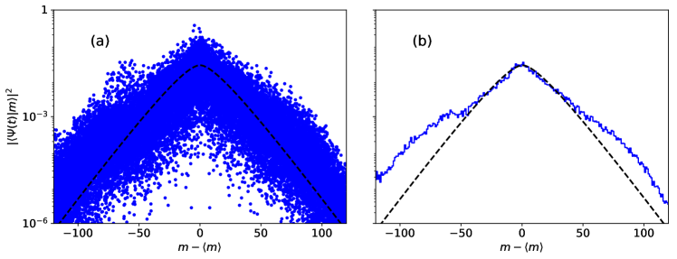
Figure 2: Average shape of momentum eigenstates evolved up to $10\times t_{\rm loc}$, for $\kappa=5.5$ in a logarithmic scale. For details about re-centering and averaging, see text. Panel (a): individual squared expansion coefficients, $|\langle m|\Psi_{m_{0}}(t)\rangle|^{2}$ for $m_{0}\in[680,782]$ (blue points). Panel (b): Histogram generated from the data shown in panel (a), by defining bins of size one and accumulating the squared expansion coefficients to yield an average probability distribution, which can be compared to Eq. (24) (blue line). In both panels, the dashed black line shows the best fit to Eq. (24), with $l_{s}=18.0$.

Wavefunction shapes

Numerically, we consider the time evolution of $|\Psi(t)\rangle$ for the sample of initial states defined above. To calculate the average shape of these states we plot the probabilities $|\langle m|\Psi(t)\rangle|^{2}$ versus the relative momentum coordinate, $m^{\prime}=m-\langle m\rangle$, where

$$\langle m\rangle=\sum_{m}m\;|\langle m|\Psi(t)\rangle|^{2}=\frac{1}{\hbar_{\rm eff}}\;\langle\Psi(t)|\hat{p}\,\Psi(t)\rangle\;.$$ (28)

We then convert the data into a histogram, defining bins of unit length around the integer values of $m^{\prime}$, summing up all probabilities which fall into the respective bin, normalizing the resulting histogram at the end.

In Fig. 2 we show the result of this procedure for $\kappa=5.5$ and $t=10\,t_{\rm loc}$ on a logarithmic scale. For each member in the ensemble, we obtain $|\langle\Psi(t)|m\rangle|^{2}$ as a function of the (centered) momentum $m^{\prime}$. The results for all members in the ensemble are shown in Panel (a). Panel (b) shows the corresponding accumulated histogram (blue line) together with the best fit to Eq. (24) (black dashed line). We find that this function agrees well with the numerical histogram in the center of the distribution. In the tails we find larger deviations, however these only have little statistical weight.

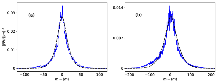
Figure 3: Comparison of the average shapes of momentum eigenstates evolved up to $10\times t_{\rm H}$, for $\kappa=5.5$ (left panel) and $\kappa=11.6$ (right panel). Here, we use a linear scale. The set of the initial states and the basis size are the same as in Fig. 2. The histograms (blue lines) and the fit function (dashed black line) are computed as in Fig. 2: $l_{s}=18.0$ for $\kappa=5.5$ and $l_{s}=41.7$ for $\kappa=11.6$.

In Fig. 3 we compare the average shapes of momentum eigenstates, evolved up to $t=10\,t_{\rm loc}$, for $\kappa=5.5$ (a) and $\kappa=11.6$ (b). The dashed curves correspond to best fitting theoretical estimate of Eq. 24. For $\kappa=5.5$ we find that the best fitting parameter, i.e. the localization length, is $l_{s}=18$, while for $\kappa=11.6$, $l_{s}=41.7$. There are some differences between the theoretical estimate and the actual profiles, as already pointed out in [8].

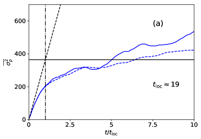
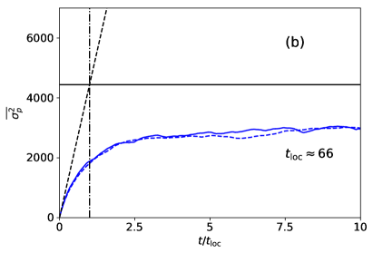
Figure 4: Ensemble averaged $\overline{\sigma^{2}_{p}}$ for the kicked rotor, as a function of discrete time $t$. Blue solid line for the small sample $m_{0}\in[680,782]$; blue dashed line for the large sample $m_{0}\in[800,1800]$. In panel (a) $\kappa=5.5$ and in panel (b) $\kappa=11.6$. For comparison we have included the classical difussion (black dashed line), the theoretical saturation of $\sigma^{2}_{p}$ (horizontal line) and $t_{\rm loc}$ (vertical line).

Momentum variance as a function of time

Here, we compute the ensemble averaged time evolution of the momentum variance $\overline{\sigma_{p}^{2}}$. The results are shown in Fig. 4 (blue lines) for $\kappa=5.5$ in panel (a) and for $\kappa=11.6$ in panel (b). For comparison, we indicate the key quantities, related to the theoretical description of the localization effect: the expected classical diffusion according to Eq. (21) (black dashed line); the expected saturation value of the momentum variance, $\sigma^{2}_{p,\rm loc}$ as defined in Eq. (26) (black solid line); and $t_{\rm loc}$ from Eq. (23) (black dash-dotted line).

In both cases, $\kappa=5.5$ [panel (a)] and $\kappa=11.6$ [panel (b)], the numerical results show notable deviations from the theoretical prediction. While the transition from the diffusive regime to localization is clearly happening at the expected time $t\sim t_{\rm loc}$, the numerical curves do not converge to the expected saturation value $\sigma^{2}_{p,\rm loc}$. On panel (a) $\kappa=5.5$, both curves (for the ensembles averages over $103$ and $10^{3}$ states) overshoot the saturation value quite notably. On panel (b) $\kappa=11.6$, by contrast, the corresponding curves remain well below. Even by analyzing much longer times and additional values for $\kappa$, we could not arrive at more consistent results. It seems that the theoretical model described above only provides a semi-quantitative description of localization in the kicked rotor.

We believe that the agreement would improve at smaller values for $\hbar_{\rm eff}$. In essence, the theoretical model is based on semi-classical arguments applied to a quantum-chaotic system. One should therefore expect an improvement when choosing smaller values for $\hbar_{\rm eff}$. Unfortunately, even reducing $\hbar_{\rm eff}$ by a half increases the computational cost prohibitively, in particular in the case of the combined system KR plus quantum walk, to be discussed below.

3 Quantum walk

In contrast to the kicked rotor (KR), the quantum walk (QW) dynamics have no “simple” Hamiltonian description. Instead, one defines a unitary operator which is applied at each discrete point in time. This description matches nicely with that of the quantum kicked rotor, where we repeatedly apply the Floquet operator $F_{\rm kr}$, defined in Eq. (19).

The QW dynamics requires an additional two-level quantum system, the quantum “coin”, which steers the quantum walker. In the simplest case, the full Hilbert space is given by the momentum coordinate and the quantum coin. Then, we define the unitary operation:

$$\begin{split}U_{\rm qw}&=S_{\rho}\;(\,U_{\rm c}\otimes\mathbbm{1}\,)\;,\\ S_{\rho}&=|0\rangle\langle 0|\otimes\hat{D}_{\rho}+|1\rangle\langle 1|\otimes\hat{D}_{-\rho}\;,\end{split}$$ (29)

where $U_{\rm c}$ is a unitary operator in the coin system, $\mathbbm{1}$ is the identity operation in the momentum coordinate, and $\hat{D}_{\rho}$ is the discrete displacement operator

$$\hat{D}_{\rho}\;|m\rangle=|m+\rho\rangle\;,\qquad D_{\rho}^{\dagger}=\hat{D}_{-\rho}\;,$$ (30)

in the momentum coordinate. Unless stated otherwise, we will restrict ourselves to the case $\rho=1$. Analogous to the kicked rotor, the evolution of a quantum state from time $t$ to time $t+1$ is obtained by

$$|\Psi(t+1)\rangle=U_{\rm qw}\;|\Psi(t)\rangle\;.$$ (31)

We will also consider cases where the unitary coin operation, $U_{\rm c}$, is chosen at random, at different sites (i.e. for different momentas) and/or at different times. In such a case, $U_{\rm c}=U_{\rm c}^{(m,t)}$ and

$$\begin{split}U_{\rm qw}^{(t)}&=S_{\rho}\;\Big{(}\,\sum_{m}U_{\rm c}^{(m,t)}\otimes|m\rangle\langle m|\,\Big{)}\;,\\ |\Psi(t+1)\rangle&=U_{\rm qw}^{(t)}\;|\Psi(t)\rangle\;.\end{split}$$ (32)

Ballistic quantum walk

One of the cases we will consider in more detail is the Hadamard quantum walk, where the coin operator is

$$U_{\rm c}=H=\frac{1}{\sqrt{2}}\begin{pmatrix}1&1\\ 1&-1\end{pmatrix}\;.$$ (33)

This choice leads to ballistic transport, which means that $\langle\hat{p}\rangle$ or $\sigma_{p}$ increase linearly in time.

For our simulations we choose the initial states as

$$\Psi(0)=\frac{1}{\sqrt{2}}\;\begin{pmatrix}1\\ \mathrm{i}\end{pmatrix}\otimes|m_{0}\rangle\;,$$ (34)

that is a symmetric eigenstate of $\sigma_{y}\otimes\mathbbm{1}$. This choice leads to two wave packets which move symmetrically and ballistically away from the initial site $|m_{0}\rangle$.

Diffusive quantum walk

The simplest way to obtain diffusive dynamics (where $\sigma^{2}_{p}$ increases linearly in time) consists in choosing $U_{\rm c}$ differently and at random at each time step. To this end, we choose $U_{\rm c}$ from the invariant distribution on SU$(2)$, which means that the corresponding probability measure is the normalized Haar measure of the group [28].

In practice, we generate random elements of this distribution by diagonalizing random Hermitian two-by-two matrices which are chosen from the Gaussian unitary ensemble (GUE) [27]. If $U$ diagonalizes such a GUE matrix, i.e.

$$H\;U=U\;\begin{pmatrix}\lambda_{1}&0\\ 0&\lambda_{2}\end{pmatrix}\;,$$

then we choose two random phases $\theta_{1}$ and $\theta_{2}$ from the uniform distribution on the interval $[0,2\pi)$ and set

$$U_{\rm c}=U\;\begin{pmatrix}\mathrm{e}^{\mathrm{i}\theta_{1}}&0\\ 0&\mathrm{e}^{\mathrm{i}\theta_{1}}\end{pmatrix}\;.$$

In this way we obtain a sequence of identically and independently distributed unitary matrices $\{\,U_{\rm c}^{(t)}=U_{\rm c}^{(m,t)}\,\}$ which are used to construct the single-step quantum-walk operators, defined in Eq. (32). Since the unitary matrices are random only in time, the evolution of the system can be calculated as

$$U_{\rm qw}^{(t)}=S_{k}\;\big{(}\,U_{\rm c}^{(t)}\otimes\mathbbm{1}\,\big{)}\;,\quad\Psi(t+1)=U_{\rm qw}^{(t)}\;\Psi(t)\;.$$ (35)

Disordered quantum walk with localization

It is also possible to observe localization in the quantum walk dynamics. For that purpose, one should associate a different coin to different sites (here momentum eigenstates). Hence, we generate a sample of random unitary matrices $\{\,U_{\rm c}^{(m)}=U_{\rm c}^{(m,t)}\,\}$ and construct a single-step quantum-walk operator. Eq. (32) then simplifies to

$$\begin{split}U_{\rm qw}&=S_{k}\;\Big{(}\,\sum_{m}U_{\rm c}^{(m)}\otimes|m\rangle\langle m|\,\Big{)}\;,\\ \Psi(t+1)&=U_{\rm qw}\;\Psi(t)\;.\end{split}$$ (36)

Disorder in space and time

Finally, we may consider the case, where we perform random and independent unitary coin transformations at different sites and different times. In this case, we generate a sample of identically and independently distributed coin transformations $\{\,U_{\rm c}^{(m,n)}\,\}$, and use Eq. (32) to compute the dynamics of the system. In this case, we expect to obtain the same type of diffusive dynamics as in the diffusive quantum walk case discussed previously.

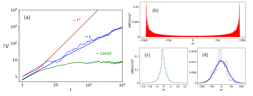
Figure 5: Panel (a): Ensemble averaged $\overline{\sigma_{p}^{2}}$ as a function of the number of time steps $t$ in a double-log plot. We depict the following cases: ballistic Hadamard quantum walk (red line), diffusive QW (blue line) and QW with disorder (green line). The dashed blue line shows site-independent random operations in time. Panels (b), (c) and (d): Final probability distributions for the respective cases shown in panel (a) with the same color code. In (d) we have included the analytical gaussian curve in black line with variance $\sigma^{2}_{p}=D_{\rho}t$ with $\rho=1$, see Eq. 38. As expected, the dynamics is equal to the classical random walk.

In Fig. 5, panel (a), we show the variance $\overline{\sigma_{p}^{2}}$ (as introduced in Fig. 4) as a function of discrete time, just as in the kicked rotor. The figure shows the result for all four types of dynamics: (i) the ballistic dynamics (red line), (ii) the diffusive dynamics with randomness in (momentum) space and time (blue solid line), (iii) the diffusive dynamics with randomness in time, only (blue dashed line), and (iv) the localized dynamics with randomness in space, only (green line). In the rest of the panels we plot the evolved state profiles after $10^{3}$ time steps for the Hadamard walk (b), the quantum walk with onsite disorder (c), and the diffusive dynamics with randomness in space and time and time only in solid and dashed lines, respectively. As expected, this reproduces earlier results e.g. those in [29], [30] for coined quantum walks and in [20] for the KR.

4 Combination of kicked rotor and quantum walk

In this section we study the competition between the two respective interference effects, strong localization present in the KR and ballistic transport in the case of the Hadamard QW (Sec. 4.1). We will then consider cases where the QW part is either diffusive or localizing (Sec. 4.2). In all cases, we combine the KR with the QW dynamics by alternatingly applying the single step unitary evolution from one model and the other:

$$F_{\rm qw,kr}=U_{\rm qw}\;U_{\rm free}^{1/2}\;U_{\rm kick}\;U_{\rm free}^{1/2}\;.$$ (37)

Note that the operators $U_{\rm free}$ and $U_{\rm kick}$ have to be extended by adding the identity in the Hilbert space of the two-level quantum coin. In addition, in the case of the diffusive quantum walk, $U_{\rm qw}$ is really time dependent as it contains different random coin operations at different times.

4.1 Combination of KR and Hadamard QW

Here, we study the dynamics generated by the Floquet operator, defined in Eq. (37), where $U_{\rm qw}$ is constructed with the Hadamard gate from Eq. (33) as coin operation, and conditional displacements by $\rho\geq 1$ steps, as defined in Eq. (30).

Naturally, we expect that the ballistic quantum walk steps will counteract the localization of the KR. However, it remains to be seen whether the localization will just be delayed and weakened (larger localization time and larger localization length) or whether it will be canceled; in the latter case the dynamics would become diffusive or ballistic. In order to arrive at a more quantitative expectation, we compute the effect of the QW part on the classical diffusion constant, as given in Eq. (8). This calculation which follows exactly the original procedure for the KR, is detailed in B. It yields the following result:

$$D_{\rho}=\rho^{2}+\frac{\kappa^{2}}{2}\big{[}\,1-2J_{2}(\kappa)+J_{2}(\kappa)^{2}\,\big{]}\;,$$ (38)

where we have assumed that $\kappa>4.5$. Hence the only change as compared to the pure KR expression consists in the addition of $\rho^{2}$. Note that for $\kappa>4.5$, the KR diffusion constant is of the order of $20$ and larger. Therefore, we would expect that a unit-step quantum walk ($\rho=1$) will have only a small effect on the KR dynamics.

In Sec. 2.3 we describe the argument which leads to an estimate of the localization length for the KR, based on the classical diffusion constant $D_{0}$. With the classical diffusion constant $D_{\rho}$ for the combined system at hand, Eq. (38), we follow the argument step by step and thereby obtain a similar estimate for the localization length of the combined system. The only problematic point is the shape of the evolving quantum states, as it is given in Eq. (24). However, as long as $\rho$ is not very large, it seems reasonable to assume that this shape remains approximately the same. We find that the result for the KR, Eq. (27), remains valid, if we simply replace the KR diffusion constant $D_{0}$ by the KR plus QW diffusion constant $D_{\rho}$.

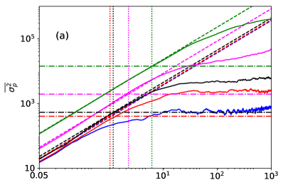
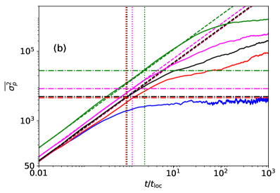
Figure 6: Variance $\overline{\sigma^{2}_{p}}$ as a function of discrete time $t$, for the kicked rotor plus Hadamard quantum walk. In panel (a), $\kappa=5.5$ and in panel (b), $\kappa=11.6$. For comparison, we have included the blue solid line corresponds to $\rho=0$, i.e. the quantum kicked rotor. The red solid line corresponds to $\rho=1$, black solid line to $\rho=2$, pink solid line $\rho=5$ and green solid line $\rho=10$. The dashed lines correspond to classical diffusion using the diffusion constant given in Eq. 38. The horizontal lines corresponds to the saturation value $\sigma_{p,{\rm loc}}^{2}$ and the vertical lines to $t_{\rm loc}$.

We numerically analyse the localization properties of the combined system in Fig. 6. Here, we plot the average momentum variance $\overline{\sigma^{2}_{p}}$ as a function of time $t$ (measured in units of the kick period) on a double-logarithmic scale. This allows us to cover a much larger range in time and momentum variance as compared to Fig. 4 (where we studied the pure KR case). Here, panel (a) shows the case $\kappa=5.5$ and panel (b) the case $\kappa=11.6$. The solid lines represent the numerical evolution of the full system for $\rho=1$ (red), $\rho=2$ (black), $\rho=5$ (pink) and $\rho=10$ (green). For completeness we have included the kicked rotor case case $\rho=0$ in blue. The dashed lines correspond to classical diffusion using the diffusion coefficient $D_{\rho}$ as given in Eq (38). The horizontal and vertical lines, in the stated color code, corresponds to the saturation variance $\sigma_{p}^{2}$ and $t_{\rm loc}$, respectively.

In all cases, the numerical results for the average momentum variance initially shows the expected diffusive behaviour, where the slope is in reasonable agreement with the diffusion constant $D_{\rho}$, obtained in Eq (38). At larger times, eventually all numerical curves deviate from the straight line, which indicates the transition to the localizing regime. However, even though we extend the simulations to very large times, namely $10^{3}$ times the KR localization time $t_{\rm loc}$, only for $\kappa=5.5$ and $\rho=1$ (and may be $\rho=2$ we find a clear tendency of the average momentum variance to saturate, and in all cases the expected theoretical saturation values are exceeded by at least an order of magnitude.

4.2 Combination of KR and different random QWs

Here, we study the dynamics when the QW part is constructed using random coin operations. We distinguish two cases, the “diffusive QW” where the coin operations are chosen at random in (momentum) space and time, see Eq. (32), and the “disordered QW”, where the coin operations are chosen at random in (momentum) space, only, see Eq. (36). In this part, we limit ourselves to unit-step displacements, $\rho=1$.

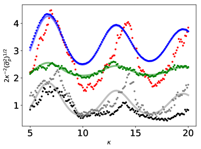
Figure 7: Scaled standard deviation of the momentum operator for the combination of the KR with different types of QW as a function of the kick strength $\kappa$. For details of its computation and the extra factor $(\kappa^{2}/2)^{-1}$ see the main text. KR only (gray points), KR plus Hadamard QW (red dots), KR plus diffusive QW (blue dots), KR plus QW with on-site disorder (green dots). The black dots correspond to the quantity $2\kappa^{-2}l_{s}$, where $l_{s}$ is obtained with the help of Eq. (26), as in Fig. 3. Where available, we included theoretical estimates (solid lines of the same color as the corresponding numerical results); for details see the main text.

To quantify the effect of the different types of QWs on the KR dynamics, we consider the square root of $\bar{\sigma}^{2}_{p}$ at the time $t=10\,t_{\rm loc}$ as a function of $\kappa$. Based on Eq. (27) we expect for the pure KR dynamics that

$$\overline{\sigma^{2}_{p}}\approx D_{0}^{2}\;,$$ (39)

while we expect deviations for the combined system, KR plus QW. To show these deviations on a convenient scale, we follow Ref. [16] and multiply $(\,\overline{\sigma^{2}_{p}}\,)^{1/2}$ by $2/\kappa^{2}$, which takes away the leading trend of the $\kappa$-dependence (in the KR case). The result is plotted in Fig. 7. Note that in all cases shown, the curves seem to oscillate around an average constant value. This means that the overall dependence on $\kappa$ remains the same as in the pure KR case. Below, we discuss the results for each case individually.

• The pure KR case is shown with gray dots. This can be compared to the solid gray line which shows the theoretical expectation based on the knowledge of the diffusion constant, as it is given in Eq. (8). The agreement is rather semi-quantitative. This is not surprising in view of the deviations found already in Fig. 4.

• For the KR plus Hadamard QW case, discussed in the previous Sec. 4.1, the result is shown with red points. Note that there is no obvious reason why the theoretical considerations which lead us to Eq. (27) could not be applied analogously to the present case, as well. Therefore, one expects the effect of the QW part onto the KR dynamics to be rather small, due to the small change in the corresponding diffusion constant (note that $\rho=1$). In fact the theoretical curve, based on Eq. (38) would be hardly distinguishable from the solid gray curve, in particular at large values of $\kappa$. In spite of this, the numerical results show very strong differences, with pronounced anharmonic oscillations and on average much larger values.

• The green points KR plus QW with on-site disorder as defined in Eq. (36). In this case, the standard deviation of the momentum seems to be approximately equal to

  $$\sqrt{\bar{\sigma}^{2}_{p}}\;\frac{2}{\kappa^{2}}\approx 2\quad:\quad\sqrt{\bar{\sigma}^{2}_{p}}\approx\kappa^{2}\;,$$ (40)

  plus some weakened remanent of the characteristic oscillations from the KR. As a guide to the eye, the solid green line shows the function $a+b\;[1-2J_{2}(\kappa)+J_{2}(\kappa)^{2}]$, with best fit values $a=1.85$ and $b=0.387$. Also here we see a strong effect, even though we just noted that in classical terms, the quantum walk part is only a small perturbation. This result also shows that combining two different mechanisms for localization does not yield stronger, but weaker localization. Indeed, for the pure localizing QW, we have $\overline{\sigma_{p}^{2}}$, which implies a very small localization length as compared to the kicked rotor case. Nevertheless the localization length of the combined system is clearly larger than in the pure KR case, for some values of $\kappa$ more than twice as large.

• Finally, the blue points show the case where the QW part is diffusive, i.e. the coin operation is random in (momentum) space and time. Here one expects that the randomness in time destroys all phase coherences between different paths, and thereby cancels strong localization. In this case, we find that the result is consistent with the assumption of normal diffusion with a diffusion coefficient equal to $D^{\prime}\approx\kappa^{2}/2$. This can be seen from the fact that at time $t=10\,t_{\rm loc}$ we find:

  $$\overline{\sigma^{2}_{p}} =10\,t_{\rm loc}\;D^{\prime}=10\;D_{0}\;D^{\prime}\;,$$

  $$\frac{2}{\kappa^{2}}\;\big{(}\,\overline{\sigma^{2}_{p}}\,\big{)}^{1/2} \approx\sqrt{10\,D_{0}}\;\frac{\sqrt{2}}{\kappa}$$

  $$\approx\sqrt{10\,\big{[}\,1-2\,J_{2}(\kappa)+2\,J_{2}(\kappa)^{2}\,\big{]}}\;.$$ (41)

  In Fig. 7 this function is shown as a solid blue line, which agrees very nicely with the corresponding numerical results (blue points).

5 Conclusions

In this work, we studied the competition between two fundamentally different interference effects, namely strong localization on the one hand and interference induced ballistic transport on the other. For that purpose, we choose the quantum kicked rotor (KR) as the base system, and add discrete-time quantum walk (QW) steps. The implementation of the QW steps requires an additional two-level system, the so called “quantum coin”. In experimental cold-atom realizations of the kicked rotor, internal atomic states may be used for that purpose. At the end, the system evolves by alternatingly applying the Floquet operator of the KR and the QW step (except for the diffusive case, the QW step is just another Floquet operator).

In a preliminary part, we review in some detail the localization properties of the KR. This study reveals some rather unexpected deviations from the theoretical expectation, namely in the case of average wavefunction shapes and the corresponding localization lengths. In the main part of the paper, we then analyse the effect of adding QW steps to the KR dynamics.

We find that only the diffusive QW is able to destroy the localization completely. The ballistic and localizing QW steps increase the localization length and as a consequence also the saturation value of the momentum variance. Using a convenient rescaling, we analyze the average momentum variance $\overline{\sigma_{p}^{2}}$ as a function of the kick-strength $\kappa$. In the pure KR case, $\overline{\sigma_{p}^{2}}$ shows an overall trend which is proportional to $\kappa^{2}$ and an additional modulation which can be described in terms of the Bessel function $J_{2}(\kappa)$. When adding ballistic QW steps, mostly the modulations are increased, by contrast, when adding localizing QW steps, the overall trend is increased while the modulations are damped. As a consequence, there are regions on the $\kappa$ axis, where the localization length is larger when the QW steps are ballistic and others (smaller ones) where it is larger when the additional QW steps are localizing.

Finally, we adapt the analytical calculation of the classical diffusion coefficient for the KR to include the ballistic QW time steps. The result shows that typically, the additional QW steps constitute a small perturbation (in classical terms) to the KR dynamics, which modify the diffusion coefficient only a ittle. This remains true for diffusive and localizing QW steps, also. In quantum mechanical terms, however, the QW steps constitute a very strong perturbation, and indeed lead to strong effects on the transport properties of the system. The adapted analytical calculation of the classical diffusion coefficient, can be used as input to the semiclassical argument which is commonly used to obtain an analytical prediction of the localization length in the KR case. However, while the argument works reasonably well for the KR, we find that it fails by orders of magnitude (c.f. Fig. 6) when applied to the combined system. A careful analysis of the semiclassical argument applied to the combined KR+QW system might shed new light on its limits of validity and even point at new options for improving its accuracy.

Appendix A Discrete Fourier transform

In principle, our Hilbert space is that of $2\pi$-periodic square integrable functions, with the scalar product

$$\langle\psi|\phi\rangle=\int_{0}^{2\pi}\mathrm{d}\theta\;\psi(\theta)^{*}\;\phi(\theta)\;.$$ (42)

Let us now choose an integer $N\gg 1$, fixed but arbitrary, and replace the exact scalar product by the following discretized version:

$$\langle\psi|\phi\rangle=\frac{2\pi}{N}\sum_{k=0}^{N-1}\psi(\theta_{k})^{*}\;\phi(\theta_{k})\;,\qquad\theta_{k}=2\pi\;\frac{k}{N}\;,$$ (43)

where the prefactor $2\pi/N$ comes from the discretization of the diferential, $\mathrm{d}\theta$. Then, for sufficiently well behaved (e.g. piecewise continous and square integrable) functions, the discretized scalar product converges to the original one, for sufficiently large $N$.

With this, we can build a new approximate Hilbert space which consists of complex finite sequences, $(\psi_{k})_{0\leq k<N}$ (which approximate the original wave functions), and the discretized scalar product we had just introduced:

$$\langle\psi|\phi\rangle=\frac{2\pi}{N}\sum_{k=0}^{N-1}\psi_{k}^{*}\;\phi_{k}\;.$$ (44)

In this new $N$-dimensional Hilbert space, consider the following $N$ state vectors:

$$|\varphi_{m}\rangle=\big{(}\,\varphi^{(m)}_{k}\,\big{)}_{0\leq k<N}\;,\quad\varphi^{(m)}_{k}=\frac{1}{\sqrt{2\pi}}\;\mathrm{e}^{2\pi\mathrm{i}\,km/N}\;,$$ (45)

for $0\leq m<N$. Note that on the one hand, these states are approximations to the angular momentum eigenstates in the original continous Hilbert space, as

$$\varphi^{(m)}_{k}=\varphi_{m}(\theta_{k})=\frac{1}{\sqrt{2\pi}}\;\mathrm{e}^{\mathrm{i}m\theta_{k}}\;,\qquad\theta_{k}=2\pi\;\frac{k}{N}\;.$$ (46)

But on the other hand they are also an exact ortho-normal basis in our approximate $N$-dimensional Hilbert space. This is because

$$\langle\varphi_{m}|\varphi_{n}\rangle=\frac{2\pi}{N}\sum_{k=0}^{N-1}\frac{1}{2\pi}\;\mathrm{e}^{2\pi\mathrm{i}\,k(n-m)/N}=\delta_{nm}\;.$$ (47)

Momentum representation

In the approximate Hilbert space, we started with the position (angle) representation,

$$|\psi\rangle\;\;\to\;\;(\psi_{k})_{0\leq k<N}\;,\qquad\psi_{k}=\psi(\theta_{k})\;,\quad\theta_{k}=2\pi\;\frac{k}{N}\;.$$ (48)

However, we can now use the new ortho-normal basis in order to obtain an alternative representation:

$$\begin{split}|\psi\rangle&=\sum_{m=0}^{N}c_{m}\;|\varphi_{m}\rangle\;,\\ c_{m}&=\langle\varphi_{m}|\psi\rangle=\frac{2\pi}{N}\sum_{k=0}^{N-1}\frac{1}{\sqrt{2\pi}}\;\mathrm{e}^{-2\pi\mathrm{i}km/N}\;\psi_{k}\;.\end{split}$$ (49)

This is precisely the discrete Fourier transform. We define this as the forward Fourier transform, which converts the position (angle) representation of a quantum state into its momentum representation (as we will see below, the states $|\varphi_{m}\rangle$ are eigenstates of the (angular) momentum operator. Finally, together with the inverse Fourier transform, we have

$$\begin{split}c_{m}&=\frac{\sqrt{2\pi}}{N}\;\sum_{k=0}^{N-1}\;\mathrm{e}^{-2\pi\mathrm{i}km/N}\;\psi_{k}\;,\\ \psi_{k}&=\frac{1}{\sqrt{2\pi}}\;\sum_{m=0}^{N-1}\;\mathrm{e}^{2\pi\mathrm{i}km/N}\;c_{m}\;.\end{split}$$ (50)

Momentum operator and momentum eigenvalues

Again, to be precise, we should call this “angular momentum operator and angular momentum eigenvalues”. In the original Hilbert space of continuous functions, the momentum eigenstates and their eigenvalues are defined as

$$\begin{split}|\varphi_{m}\rangle&=\frac{1}{\sqrt{2\pi}}\;\mathrm{e}^{\mathrm{i}m\,\theta}\;,\\ \tilde{p}\;|\varphi_{m}\rangle&=-\mathrm{i}\hbar_{\rm eff}\,\partial_{\theta}\;|\varphi_{m}\rangle=\hbar_{\rm eff}\,m\;|\varphi_{m}\rangle\;,\end{split}$$ (51)

and $m\in\mathbb{Z}$. Thus, we obtain the spectral representation of the momentum operator, as

$$\tilde{p}=\sum_{m\in\mathbb{Z}}|\varphi_{m}\rangle\;\hbar_{\rm eff}\,m\;\langle\varphi_{m}|\;.$$ (52)

In the finite dimensional Hilbert space this formula will be approximated by

$$\tilde{p}=\sum_{m=0}^{N-1}|\varphi_{m}\rangle\;\hbar_{\rm eff}\,m\;\langle\varphi_{m}|\;,$$ (53)

with the understanding, that the momentum coordinate is now periodic just in the same way as the position coordinate. In other words, the momentum eigenvalue $\hbar_{\rm eff}\,m$ is exactly the same as $\hbar_{\rm eff}\,(m-N)$. Note that this also implies that $|\varphi_{m}\rangle=|\varphi_{m-N}\rangle$, as can be verified in Eq. (45). Therefore, in order to reproduce as far as possible the momentum coordinate of the continous case, we define (here $N$ is assumed to be even)

$$\begin{split}\tilde{p}&=\!\!\sum_{m=0}^{N/2-1}\!\!|\varphi_{m}\rangle\;\hbar_{\rm eff}\,m\;\langle\varphi_{m}|+\!\!\sum_{m=N/2}^{N-1}\!\!|\varphi_{m}\rangle\;\hbar_{\rm eff}\,(m-N)\;\langle\varphi_{m}|\\ &=\sum_{m=0}^{N/2-1}|\varphi_{m}\rangle\;\hbar_{\rm eff}\,m\;\langle\varphi_{m}|+\sum_{m=-N/2}^{-1}|\varphi_{m}\rangle\;\hbar_{\rm eff}\,m\;\langle\varphi_{m}|\\ &=\sum_{m=-N/2}^{N/2-1}|\varphi_{m}\rangle\;\hbar_{\rm eff}\,m\;\langle\varphi_{m}|\;.\end{split}$$

Similarly, for $N$ being odd, we use

$$\begin{split}\tilde{p}&=\!\!\sum_{m=0}^{(N-1)/2}\!\!|\varphi_{m}\rangle\;\hbar_{\rm eff}\,m\;\langle\varphi_{m}|+\!\!\!\!\!\!\sum_{m=(N+1)/2}^{N-1}\!\!\!\!|\varphi_{m}\rangle\;\hbar_{\rm eff}\,(m-N)\;\langle\varphi_{m}|\\ &=\sum_{m=0}^{(N-1)/2}|\varphi_{m}\rangle\;\hbar_{\rm eff}\,m\;\langle\varphi_{m}|+\sum_{m=-(N-1)/2}^{-1}|\varphi_{m}\rangle\;\hbar_{\rm eff}\,m\;\langle\varphi_{m}|\\ &=\sum_{m=-(N-1)/2}^{(N-1)/2}|\varphi_{m}\rangle\;\hbar_{\rm eff}\,m\;\langle\varphi_{m}|\;.\end{split}$$

Appendix B Derivation of the classical diffusion constant for the quantum kicked rotor plus the Hadamard quantum walk

In this appendix we derive the classical diffusion constant for the KR times the Hadamard QW with extended jumps. The associated unitary evolution for the combined system is given in Eq. 37. In order to derive the diffusion constant we will follow [31] closely. Let $P(x,p,t)$ be the probability for the classical kicked rotator to be at position $x$ with momentum $p$ at time $t$. Its time evolution is given by

$$P(x,p,t)=P(x-p,p+\kappa\sin(x-p),t-1).$$ (54)

To this last equation, we can add directly the $\rho$-step classical random walk (if $\rho=1$ then we have the canonical random walk) in momentum space as

$$P(x,p,t)=\frac{1}{2}\big{[}\,P(x,p+\rho,t-1)+P(x,p-\rho,t-1)\,\big{]}\;.$$ (55)

We can solve this equation by using the method in [32], which amounts to transform $P(\cdot)$ to the characteristic function $a(\cdot)$ using the Fourier transform

$$P(x,p,t)=\sum_{m=-\infty}^{\infty}\int_{-\infty}^{\infty}\mathrm{d}k\;a(m,k,t)\;\mathrm{e}^{\mathrm{i}mx}\;\mathrm{e}^{\mathrm{i}kp}.$$ (56)

The characteristic function is

$$\begin{split}a(m,k,t)&=\cos(k+m\rho)\sum_{l=-\infty}^{\infty}J_{l}(|k+m|\kappa)\times\\ &\times a(m-l\operatorname{sign}(k),k+m,t-1),\end{split}$$ (57)

while the second moment of $p$ is obtained by evaluating

$$\langle p^{2}\rangle_{t}=-\frac{\partial^{2}}{\partial k^{2}}a(m,k,t)\bigg{|}_{m,k=0}=Dt\;.$$ (58)

The characteristic function, after $t$ steps, is found to be

$$a(m,k,T)=\cos^{t}(k\rho)\;F(J,t)\;,$$ (59)

where $F(\cdot)$ is the characteristic function for the kicked rotor only. Taking the second derivative with respect to $k$ of this function yields

$$a^{\prime\prime}=G^{\prime\prime}F+2G^{\prime}F^{\prime}+GF^{\prime\prime}$$ (60)

where $G=\cos^{t}(k\kappa)$, $G(0)=1$, $G^{\prime}(0)=0$ and $G^{\prime\prime}(0)=-\kappa^{2}t$. Thus

$$a^{\prime\prime}=-\kappa^{2}\;t\;F(0)+F^{\prime\prime}(0),$$ (61)

with $F(0)$ a constant that we fix to one. The final expression for the diffusion constant is,

$$D_{\rho}=\rho^{2}+\frac{\kappa^{2}}{2}\left(1-2J_{2}(\kappa)+J_{2}(\kappa)^{2}\right)\;.$$ (62)

Evidently, this is the same as Eq. 8 plus a contant term proportional to the size of the step squared.

References

-
[1]
P. W. Anderson,
Absence of diffusion
in certain random lattices, Phys. Rev. 109 (1958) 1492–1505.
doi:10.1103/PhysRev.109.1492.
URL https://link.aps.org/doi/10.1103/PhysRev.109.1492 -
[2]
I. García-Mata, D. L. Shepelyansky,
Delocalization
induced by nonlinearity in systems with disorder, Phys. Rev. E 79 (2009)
026205.
doi:10.1103/PhysRevE.79.026205.
URL https://link.aps.org/doi/10.1103/PhysRevE.79.026205 - [3] I. García-Mata, D. L. Shepelyansky, Nonlinear delocalization on disordered stark ladder, Stat. and Nonlin. Phys. 71 (2009) 121.
-
[4]
J. Kempe, Quantum random
walks: An introductory overview, Contemporary Physics 44 (4) (2003)
307–327.
arXiv:https://doi.org/10.1080/00107151031000110776, doi:10.1080/00107151031000110776.
URL https://doi.org/10.1080/00107151031000110776 - [5] R. Portugal, Quantum walks and search algorithms, Springer, 2013.
-
[6]
Y. Aharonov, L. Davidovich, N. Zagury,
Quantum random
walks, Phys. Rev. A 48 (1993) 1687–1690.
doi:10.1103/PhysRevA.48.1687.
URL https://link.aps.org/doi/10.1103/PhysRevA.48.1687 -
[7]
G. Casati, B. V. Chirikov, F. M. Izraelev, J. Ford,
Stochastic behavior of a quantum
pendulum under a periodic perturbation, Springer Berlin Heidelberg, Berlin,
Heidelberg, 1979, pp. 334–352.
doi:10.1007/BFb0021757.
URL http://dx.doi.org/10.1007/BFb0021757 -
[8]
F. M. Izrailev,
Simple
models of quantum chaos: Spectrum and eigenfunctions, Physics Reports
196 (5) (1990) 299 – 392.
doi:https://doi.org/10.1016/0370-1573(90)90067-C.
URL http://www.sciencedirect.com/science/article/pii/037015739090067C -
[9]
I. Manai, J.-F. m. c. Clément, R. Chicireanu, C. Hainaut, J. C. Garreau,
P. Szriftgiser, D. Delande,
Experimental
observation of two-dimensional anderson localization with the atomic kicked
rotor, Phys. Rev. Lett. 115 (2015) 240603.
doi:10.1103/PhysRevLett.115.240603.
URL https://link.aps.org/doi/10.1103/PhysRevLett.115.240603 -
[10]
C. Hainaut, I. Manai, J.-F. Clément, J. C. Garreau, P. Szriftgiser,
G. Lemarié, N. Cherroret, D. Delande, R. Chicireanu,
Controlling symmetry and
localization with an artificial gauge field in a disordered quantum system,
Nature Communications 9 (1) (2018) 1382.
URL https://doi.org/10.1038/s41467-018-03481-9 -
[11]
C. A. Ryan, M. Laforest, J. C. Boileau, R. Laflamme,
Experimental
implementation of a discrete-time quantum random walk on an nmr
quantum-information processor, Phys. Rev. A 72 (2005) 062317.
doi:10.1103/PhysRevA.72.062317.
URL https://link.aps.org/doi/10.1103/PhysRevA.72.062317 - [12] T. Nitsche, F. Elster, J. N. A. Gabris, I. Jex, Quantum walks with dynamical control: graph engineering, initial state preparation and state transfer, New J. Phys. 18 (2016) 063017.
- [13] A. G. C Groiseau, S. Wimberger, Quantum walks of kicked bose–einstein condensates, J. Phys. A 51 (2018) 275301.
-
[14]
S. Dadras, A. Gresch, C. Groiseau, S. Wimberger, G. S. Summy,
Quantum walk
in momentum space with a bose-einstein condensate, Phys. Rev. Lett. 121
(2018) 070402.
doi:10.1103/PhysRevLett.121.070402.
URL https://link.aps.org/doi/10.1103/PhysRevLett.121.070402 -
[15]
S. Dadras, A. Gresch, C. Groiseau, S. Wimberger, G. S. Summy,
Experimental
realization of a momentum-space quantum walk, Phys. Rev. A 99 (2019) 043617.
doi:10.1103/PhysRevA.99.043617.
URL https://link.aps.org/doi/10.1103/PhysRevA.99.043617 - [16] B. V. Chirikov, D. L. Shepelyansky, Localization of dynamical chaos in quantum systems, Radiofiz. 29 (9) (1986) 1041–1049.
-
[17]
D. R. Grempel, R. E. Prange, S. Fishman,
Quantum dynamics of
a nonintegrable system, Phys. Rev. A 29 (1984) 1639–1647.
doi:10.1103/PhysRevA.29.1639.
URL https://link.aps.org/doi/10.1103/PhysRevA.29.1639 -
[18]
L. E. Reichl,
The
transition to chaos: conservative classical systems and quantum
manifestations, 2nd Edition, Springer-Verlag, New-York, 2004.
URL https://www.amazon.com/Transition-Chaos-Conservative-Classical-Manifestations/dp/0387987886?SubscriptionId=0JYN1NVW651KCA56C102&tag=techkie-20&linkCode=xm2&camp=2025&creative=165953&creativeASIN=0387987886 - [19] Viv Kendon, Decoherence in quantum walks – a review, Mathematical Structures in Computer Science, 17 (6), 1169–1220 (2007).
- [20] Weiß, Marcel and Groiseau, Caspar and Lam, W. K. and Burioni, Raffaella and Vezzani, Alessandro and Summy, Gil S. and Wimberger, Sandro, Steering random walks with kicked ultracold atoms, Phys. Rev. A, 92 (3), 033606 (2015).
- [21] D. Delande, Kicked rotor and anderson localization, Boulder school on Condensed Matter Physics (2013).
- [22] M. Abramowitz, I. A. Stegun (Eds.), Handbook of mathematical functions, Dover publications, inc., New York, 1970.
-
[23]
S. Fishman, D. R. Grempel, R. E. Prange,
Chaos, quantum
recurrences, and anderson localization, Phys. Rev. Lett. 49 (1982) 509–512.
doi:10.1103/PhysRevLett.49.509.
URL https://link.aps.org/doi/10.1103/PhysRevLett.49.509 - [24] D. S. BV Chirikov, FM Izrailev, Dynamical stochasticity in classical and quantum mechanics, Sov. Scient. Rev. C 2 (1981) 209–267.
-
[25]
B. Chirikov, F. Izrailev, D. Shepelyansky,