Positive-energy spectra of atomic hydrogen in a magnetic field with an adiabatic-basis-expansion method

Abstract

The problem of photoionization of atomic hydrogen in a white-dwarf-strength magnetic field is revisited to understand the existing discrepancies in the positive-energy spectra obtained by a variety of theoretical approaches reported in the literature. Oscillator strengths for photoionization are calculated with the adiabatic-basis-expansion method developed by Mota-Furtado and O’Mahony [Phys. Rev. A 76, 053405 (2007)]. A comparative study is performed between the adiabatic-basis-expansion method and our previously developed coupled-channel theory [Phys. Rev. A 94, 033422 (2016)]. A detailed analysis of the positive-energy spectra obtained here and those from other theoretical approaches shows that the adiabatic-basis-expansion method can produce more accurate positive-energy spectra than other reported approaches for low field strengths.

I Introduction

Understanding the behavior of atoms in the presence of magnetic fields has been a subject of considerable interest, since Zeeman experimentally discovered the splitting of atomic spectral lines in a magnetic field at the end of the 19th century Garstang . From then on, a great deal of effort has been devoted to the study of magnetized atomic systems. Many early attempts in this aspect were made within the framework of classical theory, before the establishment of quantum mechanics gave researchers a deeper insight into the dynamics of magnetized atoms. Perturbation theory achieved prominent success in quantitatively explaining the splitting of spectral lines of hydrogen atoms in a weak magnetic field in the early stages of quantum mechanics. However, it took a long time to understand the behavior of atoms in a strong magnetic field, i.e., the so-called quadratic Zeeman effect.

A spectroscopic experiment on highly excited barium atoms in a strong magnetic field of laboratory strength, reported by Garton and Tomkins Garton in 1969, stimulated interest in the quadratic Zeeman effect. Such interest was reinforced by a growing number of subsequent experiments on other strongly-magnetized atoms (see, e.g., Refs. Holle ; Iu and references therein). The regular quasi-Landau resonance structures observed in the negative-energy region close to the ionization thresholds were interpreted by the semiclassical theory developed by Du and Delos Du . The diamagnetic Rydberg spectra of the alkali-metal atoms in the positive-energy region were also reproduced by fully quantum-mechanical approaches OMahony ; Watanabe . Undoubtedly, the study on the structures and dynamics of atoms in the presence of magnetic fields has made significant headway up to the 1990s.

The discovery of superstrong magnetic fields in white-dwarf stars with field strengths $10^{2}-10^{5}$ T and neutron stars with field strengths $10^{7}-10^{9}$ T reinforced interest in theoretical investigations of atoms in the presence of high magnetic fields Garstang ; Ferrario2015 . In astronomy and astrophysics, spectra from highly accurate theories are indispensable for determining the size of magnetic fields in the atmospheres of white-dwarf and neutron stars. So far, many efforts have been dedicated to developing nonperturbative theories and numerical methods to calculate properties of magnetized atoms (see, e.g., Ref. Ruder1994 and references therein). A multiconfiguration Hartree-Fock method was developed to calculate the properties of magnetized hydrogen atoms Rosner1984 ; Forster1984 . This method provides a tool to model spectral lines of bound-bound transitions for hydrogen atoms in magnetic fields of both white dwarfs and neutron stars. More recently, a finite-basis-size method Zhao2007 was extended to calculate discrete spectral lines of the Lyman, Balmer, and Paschen series for magnetized hydrogen atoms Zhao2019 ; Zhao2020 .

At this time, it has become possible to model discrete spectra of hydrogen atoms in an arbitrary magnetic field, based on the above-mentioned theoretical approaches. While this represents significant progress in astrophysical applications, theories for describing multielectron atoms in a magnetic field are still very scarce, and far from satisfying the demands of analyzing the spectra observed in magnetic white dwarfs and neutron stars. The origin of the problem can be attributed to the difficulties of treating electron correlations in a strong magnetic field. Very recently, the Zeeman splitting lines of multielectron atoms, such as He, Ca, Mg, Fe, and Na, were discovered in the atmospheres of magnetic white dwarfs Ferrario2020 . Consequently, it is inevitable to develop theories and numerical methods to calculate the properties of strongly magnetized multielectron atoms.

As mentioned above, identifications of discrete spectra of some magnetized atoms have been successful. However, the analysis of continuum spectra observed from magnetic celestial objects suffers from the lack of accurate photoionization cross sections. To our knowledge, no theoretical study on photoionization of highly magnetized multielectron atoms has yet been reported in the literature, and only a few theoretical approaches have been presented for describing bound-free transitions of hydrogen atoms in magnetic fields with white-dwarf-field strengths. Alijah et al. Alijah developed a theoretical approach based on multichannel quantum defect theory to describe bound-free transitions for magnetized hydrogen atoms. The wave functions for the continuum states were obtained by numerically solving the coupled Schrödinger equations. The photoionization spectrum from the ground state was published for a magnetic field of 2,000 T, and a Rydberg series of resonance states was identified. The authors expressed confidence that an extension to field strengths lower than 2,000 T was possible with some modifications of their approach.

Delande et al. Delande presented a complex-rotation method to calculate positive-energy spectra of hydrogen atoms in a magnetic field. The photoionization spectrum from the ground state in a magnetic field of 23,500 T was reported. This spectrum has become the benchmark for testing theories of bound-free transitions in a strong magnetic field. Merani et al. Merani developed a complex-coordinate method similar to that of Delande et al. to produce the vast amount of data on photoionization cross sections as a function of field strengths and energies that are required for the analysis of spectra observed in magnetic celestial objects. Balmer and Paschen bound-free opacities were determined from the obtained cross sections. Zhao and Stancil Zhao2006 presented a computational scheme based on the complex-rotation method using a mixed Slater-Landau basis to yield continuum spectra of magnetized hydrogen atoms. In order to describe atomic hydrogen diamagnetism, Wang and Greene Wang combined $R$-matrix theory with multichannel quantum defect theory to construct a theoretical approach to calculate photoionization cross sections of hydrogen atoms in magnetic fields with strengths of $10^{3}-10^{4}$ T. However, this approach did not reproduce the continuum spectrum at 2,000 T published by Alijah et al. Alijah .

The discrepancies of the continuum spectrum at 2,000 T from the two theoretical studies mentioned above motivated us to further explore the dynamics of bound-free transitions in a strong magnetic field. A coupled-channel theory was developed for this purpose Zhao2016 , but this theory could reproduce neither the spectrum of Alijah et al. Alijah nor that of Wang and Greene Wang . This unexpected result stimulated us to revisit the problem of photoionization of atomic hydrogen in a white-dwarf-strength magnetic field. In the present work, we adopt the adiabatic-basis-expansion method established by Mota-Furtado and O’Mahony OMahony2007 to perform such an investigation. Our purpose is to elucidate potential reasons for the discrepancies in the continuum spectra at 2,000 T obtained in the various calculations.

This manuscript is organized as follows. Section II is devoted to sketching the adiabatic-basis-expansion method developed by Mota-Furtado and O’Mahony OMahony2007 , which is used to study the photoionization of hydrogen atoms in a strong magnetic field in the current paper. In Sect. III, the adiabatic-basis-expansion method is applied to calculating continuum spectra of magnetized hydrogen atoms. A comparative study of these spectra close to the ionization thresholds is performed between this method and our previously developed coupled-channel theory Zhao2016 . The predicted continuum spectra are also compared to those from other theoretical approaches. A detailed analysis of the existing discrepancies among the continuum spectra obtained by the different theoretical methods is presented in this section. Section IV summarizes the results of the current study and our main conclusions regarding photoionization of hydrogen atoms in strong magnetic fields.

Atomic units are used throughout this paper unless otherwise noted.

II Sketch of the theoretical method

The adiabatic-basis-expansion method developed to study photoionization of hydrogen atoms in the presence of magnetic fields was formulated by Mota-Furtado and O’Mahony in Ref. OMahony2007 , where more theoretical details can be found. Here we only outline the general flow of arguments and point out significant features relevant to the current work.

Suppose a hydrogen atom in some initial state is placed in a magnetic field $B$ pointing along the $z$ axis. The Hamiltonian $H$ for this atomic system is written in the form

$$\widehat{H}=-\frac{1}{2}\nabla^{2}-\frac{1}{r}+\frac{\gamma}{2}({\hat{\ell}}_{z}+2{\hat{s}}_{z})+\frac{1}{8}{\gamma^{2}}r^{2}\sin^{2}\theta,$$ (1)

where $\gamma=B/B_{0}$ is the magnetic field strength in atomic units, $i.e.$, in multiples of $B_{0}\approx 2.35\times 10^{5}$ T, ${\hat{\ell}}_{z}$ and ${\hat{s}}_{z}$ are the $z$ components of the orbital and spin angular momenta, respectively, the third term (linear in $\gamma$) is the paramagnetic potential, and the fourth term (quadratic in $\gamma$) is the diamagnetic potential. For this atomic system, the orbital angular momentum is not a good quantum number specified by $\ell$, but its projection on the $z$ axis is a good quantum number specified by $m$. Furthermore, the $z$ parity of the eigenstates, denoted by $\pi_{z}$ below, is conserved. Here $\pi_{z}$ and $m$ are adopted to identify the hydrogen atomic states, labeled by $m^{\pi_{z}}$, in a magnetic field.

When such an atom is irradiated by a beam of polarized light, it may absorb a photon and then be ionized. The electron wave produced by the ionization process propagates from the inner to the outer region. The entire configuration space is divided into multiple radial sectors with radii $a\to a_{1}\to a_{2},\cdot\cdot\cdot,\to a_{N-1}\to a_{N}=b$, where $N$ is the number of the sectors, while $a$ and $b$ are the inner and outer radius, respectively. To begin with, the local adiabatic basis is constructed in each sector, and then the radial wave functions or the $R$-matrix are propagated from the inner region to the asymptotic region, sector by sector. Finally, a two-dimensional matching to the $R$-matrix in the asymptotic region, where the solutions of the coupled Schrödinger equations in cylindrical coordinates are attainable, is performed to extract the reactance matrices. Throughout this paper, we will use as much as possible the same symbols as in Ref. OMahony2007 , where the details of the adiabatic-basis-expansion method are given.

II.1 Adiabatic eigenstates

The first step to develop the adiabatic-basis-expansion method is to construct the local adiabatic basis set. The adiabatic Hamiltonian $\widehat{H}_{ad}$ is written as

$$\widehat{H}_{ad}(r_{a}^{n};\theta,\phi)=\frac{\hat{\ell}^{2}}{2(r_{a}^{n})^{2}}-\frac{1}{r_{a}^{n}}+\frac{1}{8}\gamma^{2}(r_{a}^{n})^{2}\sin^{2}\theta,$$ (2)

where $\hat{\ell}$ is the orbital angular momentum operator and $r_{a}^{n}$ is the radius of the $n$th sector lying in the interval $a_{n-1}<r_{a}^{n}<a_{n}$. It is often taken as the midpoint of the sector. By selecting a basis set of spherical harmonics and calculating each matrix element of the adiabatic Hamiltonian in the basis set selected, one can diagonalize the resulting adiabatic Hamiltonian matrix and thereby obtain the adiabatic eigenstates $\varphi_{\lambda}(r_{a}^{n};\theta,\phi)$ and eigenvalues $U_{\lambda}(r_{a}^{n})$. The adiabatic eigenvalue curves obtained can be plotted as a function of the radius $r$. Such curves illustrate equal energy spacing of Landau states at large $r$, which is regarded as the asymptotic region where the two-dimensional matching can begin.

II.2 $\bm{R}$-matrix propagation

A basis set of orthogonal radial functions is essential in order to calculate the radial wave functions of the Hamiltonian (1) in each sector. Such a basis set was defined by Mota-Furtado and O’Mahony OMahony2007 in terms of Legendre polynomials, while the full basis set of the Hamiltonian (1) consists of the product of the orthogonal radial functions, denoted by $f_{j}(r)$ with $j=1,2,3,\dotso$, and the adiabatic functions in one sector, $\varphi_{\lambda}(r_{a}^{n};\theta,\phi)$. With the basis set obtained, the solution of the Hamiltonian equation

$$(\widehat{H}-\varepsilon)\Psi=0$$ (3)

is practicable by matrix diagonalization. However, $\widehat{H}$ is not Hermitian in the individual sectors, due to nonvanishing surface terms. Equation (3), therefore, has to be revised to ensure the hermiticity of the Hamiltonian operator involved.

Adding $\widehat{L}\Psi$ on both sides of the above equation, Eq. (3) is rewritten as

$$(\widehat{H}+\widehat{L}-\varepsilon)\Psi=\widehat{L}\Psi.$$ (4)

Here $\widehat{L}$ is the Bloch operator introduced in Ref. OMahony2007 to guarantee that $\widehat{H}$ + $\widehat{L}$ is Hermitian. The above equation can be formally solved yielding

$$\Psi=(\widehat{H}+\widehat{L}-\varepsilon)^{-1}\widehat{L}\Psi.$$ (5)

Here $(\widehat{H}+\widehat{L}-\varepsilon)^{-1}$ is the Green’s function given by

$$(\widehat{H}+\widehat{L}-\varepsilon)^{-1}=\sum_{k}\frac{|\psi_{k}\rangle\langle\psi_{k}|}{E_{k}-\varepsilon},$$ (6)

where $\psi_{k}$ and $E_{k}$ are eigenfunctions and eigenvalues of the operator $\widehat{H}+\widehat{L}$ within one sector. They are obtained in each sector by diagonalizing the matrix equation of $\widehat{H}+\widehat{L}$ with matrix elements calculated in the basis set $\{f_{j}(r)\varphi_{\lambda}(r_{a}^{n};\theta,\phi)\}$. Then each $\psi_{k}$ in the $n$th sector is expressed as

$$\psi_{k}=\sum_{jk}c_{j\lambda}^{k}\frac{1}{r}f_{j}(r)\varphi_{\lambda}(r_{a}^{n};\theta,\phi).$$ (7)

Substituting Eq. (6) into Eq. (5) yields

$$\Psi=\sum_{k}\frac{|\psi_{k}\rangle\langle\psi_{k}|\widehat{L}|\Psi\rangle}{E_{k}-\varepsilon}.$$ (8)

The total continuum wave function $\Psi$ at any energy in the $n$th sector can be formally written as

$$\Psi=\sum_{\lambda}\frac{1}{r}F_{\lambda}(r)\varphi_{\lambda}(r_{a}^{n};\theta,\phi).$$ (9)

The right-hand sides of the above two equations are equal. Substituting the Bloch operator given in Ref. OMahony2007 and Eq. (7) into the resulting equation, multiplication of the equation by $\varphi_{\lambda^{\prime}}^{*}(r_{a}^{n};\theta,\phi)$, and integration over $\theta$ and $\phi$ yields equations to relate the functions and their derivatives at the boundaries of the $n$th sector. In compact matrix notation, we write these equations as

$$F(a_{n-1})={\mathscr{R}}_{2}^{n}F^{\prime}(a_{n})-{\mathscr{R}}_{1}^{n}F^{\prime}(a_{n-1});$$ (10)

$$F(a_{n})={\mathscr{R}}_{4}^{n}F^{\prime}(a_{n})-{\mathscr{R}}_{3}^{n}F^{\prime}(a_{n-1}).$$ (11)

Here ${\mathscr{R}}_{i}^{n}$ with $i=1,2,3,4$ are the sector $R$ matrices defined in Ref. OMahony2007 , where $\bm{r}_{i}^{n}$ is used instead of ${\mathscr{R}}_{i}^{n}$. While one can propagate the radial wave functions from one sector to its adjacent sector using the above two equations, it is more convenient to propagate the $R$ matrix, which relates the radial wave function and its derivative, $F(a_{n})=R(a_{n})F^{\prime}(a_{n})$. The relationship between the $R$ matrices on the inner and outer boundaries of the $n$th sector is derived from Eqs. (10) and (11) as

$$R(a_{n})={\mathscr{R}}_{4}^{n}-{\mathscr{R}}_{3}^{n}[{\mathscr{R}}_{1}^{n}+R(a_{n-1})]^{-1}{\mathscr{R}}_{2}^{n}.$$ (12)

It should be emphasized that $R(a_{n})$ and $R(a_{n-1})$ are represented in the same adiabatic basis set as the sector $R$ matrices. Since the adiabatic basis varies from one sector to another, it is essential to change the basis representation of the $R$ matrix for its propagation. The matrix elements of the transformation matrix are

$$(T^{n-1,n})_{\lambda\lambda^{\prime}}=\langle\varphi_{\lambda}(r_{a}^{n};\theta,\phi)|\varphi_{\lambda^{\prime}}(r_{a}^{n};\theta,\phi)\rangle.$$ (13)

The $R$ matrix transformed from one sector to its adjacent sector is given by

$$\overline{R}=\widetilde{T}^{n-1,n}RT^{n-1,n},$$ (14)

where $\widetilde{T}^{n-1,n}$ is the transpose of $T^{n-1,n}$.

Equations (12) and (14) can be used to propagate the $R$ matrix sector by sector. Such a propagation starts at $r=a$, where the $R$ matrix of the field-free hydrogen atom can be calculated using Seaton’s code Seaton2002 , and stops in the asymptotic region with $r=b$.

Mota-Furtado and O’Mahony OMahony2007 actually provided another scheme to propagate the radial wave functions or the $R$ matrices. Their scheme adopts the global sector $R$ matrices derived in Ref. Stechel and denoted by ${\mathcal{R}}_{i}^{n}$ in the present paper. The radial wave function and its derivative on the boundaries of the first sector and the $n$th sector are related by

$$F(a)={\mathcal{R}}_{2}^{n}F^{\prime}(a_{n})-{\mathcal{R}}_{1}^{n}F^{\prime}(a);$$ (15)

$$F(a_{n})={\mathcal{R}}_{4}^{n}F^{\prime}(a_{n})-{\mathcal{R}}_{3}^{n}F^{\prime}(a).$$ (16)

We note that the sector-by-sector propagation is hidden in the global sector $R$ matrices. From the above two equations, one can obtain an expression to relate the $R$ matrices on the boundaries of the first sector and the final sector,

$$R(b)={\mathcal{R}}_{4}^{n}-{\mathcal{R}}_{3}^{n}[{\mathcal{R}}_{1}^{n}+R(a)]^{-1}{\mathcal{R}}_{2}^{n}.$$ (17)

In the current work, we used the scheme with the global sector $R$ matrices as given in Eq. (17) to propagate the $R$ matrix.

II.3 Two-dimensional matching in the asymptotic region

Since the electron motion in $\rho$ is bound, the Coulomb potential for large $z$ can be expanded into a series,

$$-\frac{1}{\sqrt{z^{2}+\rho^{2}}}=-\frac{1}{z}+\frac{\rho^{2}}{2z^{3}}+O(\frac{1}{z^{5}})+\cdot\cdot\cdot$$ (18)

The Hamiltonian as specified by Eq. (1) becomes separable in cylindrical coordinates as $z\to\infty$. It is written as

$$\widehat{H}=-\frac{1}{2}\frac{d^{2}}{dz^{2}}-\frac{1}{z}+\frac{\rho^{2}}{2z^{3}}+O(\frac{1}{z^{5}})+\widehat{H}_{L},$$ (19)

where $\widehat{H}_{L}$ is the Hamiltonian for the Landau states $\Phi_{i}(\theta,\phi)$. The potential (18) can be approximated by $-1/z$ for sufficiently large $z$, where the $j$th linearly independent solution of the Hamiltonian system (19) is written as

$${\Psi}_{j}=\sum_{i}\Phi_{i}(\rho,\phi)[s_{i}(z)\delta_{ij}+c_{i}(z)K_{ij}].$$ (20)

Here $s_{i}(z)$ and $c_{i}(z)$ are the energy-normalized regular and irregular Coulomb functions defined by Seaton Seaton , while $K_{ij}$ are the matrix elements of the reactance matrix $K$, which is determined by a two-dimensional matching procedure. The functions $s_{i}(z)$ and $c_{i}(z)$ are calculated using the code written in Ref. Zhao2016 . We performed the matching on an arc at $r=b$.

Note that an extra index $j$ was added in $F_{\lambda}$ and $\Psi$ to label the solution specified in Eq. (9). We set Eq. (9) with $j$ added and Eq. (20) equal to each other and then project both sides of the resulting equation onto $\varphi_{\lambda}(r;\theta,\phi)$. This yields

$$\frac{1}{r}F_{\lambda j}(r)=\sum_{i}\left[P_{\lambda i}(r)\delta_{ij}+Q_{\lambda i}(r)K_{ij}\right],$$ (21)

with

$$P_{\lambda i}(r)=r\int\varphi_{\lambda}^{*}(r;\theta,\phi)\Phi_{i}(\rho,\phi)s_{i}(z)d\Omega$$ (22)

and

$$Q_{\lambda i}(r)=r\int\varphi_{\lambda}^{*}(r;\theta,\phi)\Phi_{i}(\rho,\phi)c_{i}(z)d\Omega.$$ (23)

The derivatives of $P_{\lambda i}(r)$, $Q_{\lambda i}(r)$, and $F_{\lambda j}(r)$ with respect to $r$ can be worked out from the above three equations. Using the definition of the $R$ matrix, one obtains

$$R=[P+QK][P^{\prime}+Q^{\prime}K]^{-1},$$ (24)

where the $R$ matrix at $r=b$ is calculated from Eq. (17). Rearranging the above equation yields

$$K=-[RQ^{\prime}-Q]^{-1}[RP^{\prime}-P].$$ (25)

We note that our two-dimensional matching procedure given above is similar to that employed by Watanabe and Komine Watanabe , but it differs from that of Mota-Furtado and O’Mahony OMahony2007 .

II.4 Differential oscillator strength and cross sections

The differential oscillator strength for the photoionization process from an initial state $\Psi_{i}$ with energy $\varepsilon_{i}$ to a final state $\Psi_{j}^{-}$ with energy $\varepsilon$ is given by

$$\frac{df_{j,i}}{d\varepsilon}=2(\varepsilon-\varepsilon_{i})|\langle\Psi_{j}^{-}|D|\Psi_{i}\rangle|^{2},$$ (26)

where $D$ is the electric dipole operator in the length gauge and $\Psi_{j}^{-}$ is the energy-normalized incoming wave function. If the influence of the magnetic field on the atom is negligibly small in the region close to the nucleus, $\Psi_{j}^{-}$ in this region reduces to

$$\Psi_{j}^{-}=\sum_{\ell}\frac{1}{r}F^{-}_{\ell j}(r)Y_{\ell m}(\theta,\phi),$$ (27)

where $F^{-}_{\ell j}$ can be written as a product of the field-free solution, which is the diagonal matrix with elements $S_{ij}=s_{i}\delta_{ij}$, and a constant denoted by $A^{-}$, which should be determined by means of the asymptotic solution. From Eq. (15), we have

$$[S(a)+{\mathcal{R}}_{1}^{N}S^{\prime}(a)]A^{-}={\mathcal{R}}_{2}^{N}F^{\prime-}(b),$$ (28)

where the $F^{\prime-}(b)$ are the energy-normalized incoming asymptotic solutions, which are constructed from the standing-wave solutions given in Sec. II C. The physical reactance matrix is recovered using Seaton’s quantum-defect theory Seaton from the reactance matrix $K$. The coefficients $A^{-}$ are obtained by solving the above equation. Note that they are both field- and energy-dependent.

Using the obtained coefficients $A^{-}$, Eq. (26) is rewritten as

$$\frac{df_{j,i}}{d\varepsilon}=|A^{-}_{j}|^{2}\frac{f_{j,i}}{d\varepsilon}{\bigg{|}}_{B=0},$$ (29)

where $\frac{\displaystyle f_{j,i}}{\displaystyle d\varepsilon}{\big{|}}_{B=0}$ represents the field-free differential oscillator strength. The total differential oscillator strength is an observable quantity. It is obtained by summing the differential oscillator strengths for photoionization to the individual states according to

$$\frac{df_{i}}{d\varepsilon}=\sum_{j}\frac{f_{j,i}}{d\varepsilon}.$$ (30)

The photoionization cross section is related to the total differential oscillator strength by

$$\sigma_{i}(\varepsilon)=2\pi^{2}\alpha\frac{df_{i}}{d\varepsilon},$$ (31)

where $\alpha$ is the fine-structure constant.

III Results and discussion

This section presents results of our investigation regarding photoionization of hydrogen atoms in a white-dwarf-strength magnetic field, as obtained with the adiabatic-basis-expansion method outlined above. For each atomic state $m^{\pi_{z}}$ with a given magnetic field, we diagonalize the adiabatic Hamiltonian ${\widehat{H}}_{ad}$ in a basis set of spherical harmonics as a function of the radius and then plot the resulting adiabatic eigenvalue curves. We utilize these curves to determine the asymptotic radius $b$, where a two-dimensional matching to the asymptotic solutions is performed. Figure 1 depicts the lowest ten adiabatic eigenvalue curves for the atomic state $m^{\pi_{z}}=0^{-}$ at $\gamma=0.01$ a.u. These curves begin to display an equal energy spacing of Landau levels from $r\approx 200$ a.u. onwards. We vary $r$ around 200 a.u. to check the convergence of the predicted photoionization oscillator strengths and finally fix the outer radius $b$.

Figure 1: Lowest ten adiabatic eigenvalue curves as a function of radius for the atomic state $m^{\pi_{z}}=0^{-}$ at $\gamma=0.01$ a.u.

A spectrum for photoionization into the final continuum state $m^{\pi_{z}}=0^{-}$ from the ground state at $\gamma=0.1$ a.u. was presented by Mota-Furtado and O’Mahony OMahony2007 . We recalculated this spectrum with energies covering the range from the first up to the third Landau thresholds using the current adiabatic-basis-expansion method, while our asymptotic solutions differ from those of Ref. OMahony2007 . Nevertheless, one would expect that our calculations produce similar spectra to theirs. Unfortunately, we do not have access to their actual data, and therefore no detailed comparison can be made. However, visual inspection of their Fig. 6 indeed suggests very good agreement. Furthermore, we performed a comparison with the available spectral data from the coupled-channel theory Zhao2016 and found excellent agreement over the entire energy range covered. Figure 2 displays the part of the Rydberg spectrum right below the second and third Landau thresholds from the two methods to illustrate this excellent agreement.

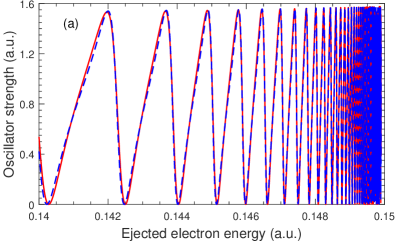
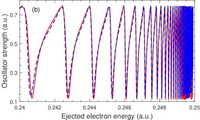
Figure 2: Comparison of the Rydberg spectrum for photoionization into the final continuum state $m^{\pi_{z}}=0^{-}$ from the ground state of hydrogen atoms in a magnetic field with $\gamma=0.1$ a.u., just below the second (a) and third (b) Landau thresholds. The red solid and blue dashed curves represent the results from the current adiabatic-basis-expansion method and the coupled-channel theory Zhao2016 , respectively.

This agreement shows the reliability of the current theoretical method and provides confidence in revisiting the problem of photoionization of atomic hydrogen in a magnetic field of 2,000 T with the adiabatic-basis-expansion method. Note that the continuum spectra at 2,000 T reported in the literature are in significant disagreement with each other Alijah ; Wang ; Zhao2016 .

We first calculated oscillator strengths for photoionization into the final continuum state $m^{\pi_{z}}=1^{+}$ from the ground state of atomic hydrogen in a magnetic field of 2,000 T. We sought the outer radius $b$ by plotting the adiabatic eigenvalue curves for the atomic state $m^{\pi_{z}}=1^{+}$ and found $b\approx 220$ a.u. from the asymptotic behavior of these curves. As mentioned above, the convergence of the predicted oscillator strengths was checked by varying $b$ in the vicinity of 220 a.u. The stability of the results was checked further by varying other parameters, such as the inner radius $a$, the number of channels involved, and the number and size of the sectors.

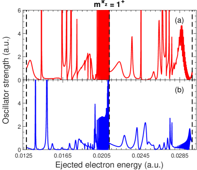
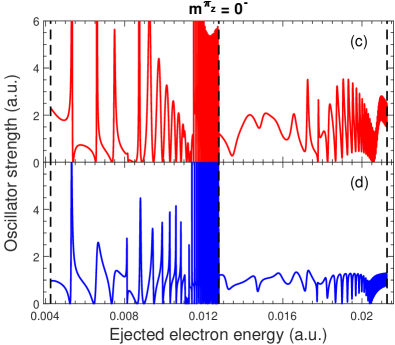
Figure 3: Comparison of photoionization spectra for ground-state hydrogen atoms in a magnetic field of $B$ = 2,000 T obtained with the current adiabatic-basis-expansion method (a,c) and the coupled-channel theory (b,d). The two photoionization processes into the various final continuum states are labeled $m^{\pi_{z}}=1^{+}$ and $m^{\pi_{z}}=0^{-}$, respectively. The ejected-electron energies cover the range from the first to the third Landau thresholds, indicated by the dashed vertical lines, for both photoionization processes.

The calculated spectrum from the first to the third Landau ionization thresholds is shown in Fig. 3 (a). The spectrum in the same energy region was also calculated using the coupled-channel theory Zhao2016 and is plotted in Fig. 3 (b) for comparison. The results from these two methods are in qualitative agreement, but pronounced discrepancies between the two spectra are clearly visible in the details. A broad resonance structure underlying the Rydberg resonance peaks right below the third Landau threshold can be seen in both of these spectra, but their positions, widths, and heights differ. The broad resonance was attributed by Alijah et al. Alijah to the downward-shifted $n=8$ state of the fourth Landau channel.

The level of disagreement displayed in Figs. 3 (a,b) was unexpected. On the other hand, the current calculations do not reproduce the part of the spectrum right below the third Landau threshold reported by Alijah et al. Alijah either. Finally, our Rydberg spectrum below the third Landau threshold also differs from that of Wang and Greene Wang . Using the $R$-matrix approach, which is constructed within the framework of multichannel quantum-defect theory, to analyze the close-coupling calculations of Alijah et al. Alijah in detail, Wang and Greene concluded that the box size $z_{0}=50$ a.u used by Alijah et al. is too small.

We then calculated photoionization into the final continuum state $m^{\pi_{z}}=0^{-}$ from the ground state of hydrogen atoms in a magnetic field of 2,000 T with both the current method and the coupled-channel theory Zhao2016 . The obtained oscillator strengths are displayed as a function of ejected electron energy in Figs. 3 (c) and (d). We again expected better agreement in the details than what is observed in these figures. Only qualitative agreement between the results from the two theoretical methods is still visible over the entire energy region covered.

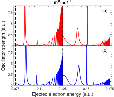
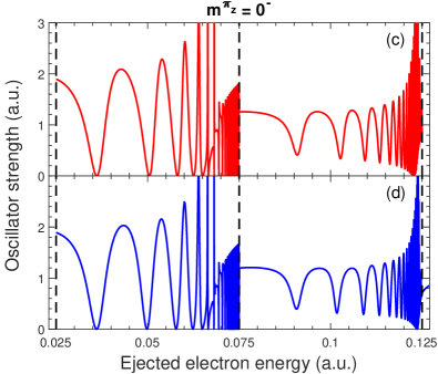
Figure 4: Same as Fig. 3, but with $\gamma=0.05$ a.u.

In order to better understand the discrepancies of the Rydberg spectra shown in Fig. 3, we calculated photoionization spectra of hydrogen atoms in magnetic fields with different field strengths. Figure 4 displays our calculated oscillator strengths in a magnetic field with $\gamma$ = 0.05 a.u. as a function of the ejected-electron energy. We assume that magnetized hydrogen atoms in the ground state are irradiated by beams of circularly and linearly polarized light, respectively, and then ionized into the two final continuum states $m^{\pi_{z}}=1^{+}$ and $0^{-}$. The results from the coupled-channel theory are also shown in this figure for comparison. Good agreement between the results from the two methods is evident for both photoionization processes, although some small discrepancies exist. One readily sees, for example, small shifts of the resonance positions near $\varepsilon=0.078$, 0.14, and 0.15 a.u., as well as a minor discrepancy in the resonance width near $\varepsilon$ = 0.078 a.u.

The parts of the spectrum right below the Landau thresholds displayed in Fig. 4 are not sufficiently resolved. It is, however, helpful to display a detailed comparison of these parts in order to understand the discrepancies between the Rydberg spectra in Fig. 3. Such a detailed comparison right below the second and third Landau thresholds is presented in Fig. 5. The resonances associated with high-lying Rydberg states are becoming increasingly narrow as the ejected electron energies approach the Landau threshold. Discrepancies in the heights of these Rydberg resonances obtained by the two theoretical methods can be seen for the two photoionization processes into the two final continuum states $m^{\pi_{z}}=1^{+}$ and $0^{-}$, but their positions, widths, and overall energy dependence are in good agreement with each other.

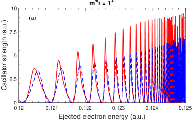
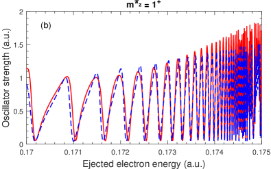
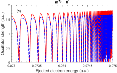
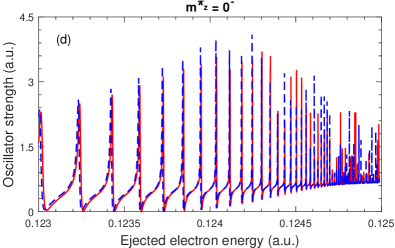
Figure 5: Detailed comparison of Rydberg spectra, as given in Fig. 4, between the current adiabatic-basis-expansion method (red solid curves) and the coupled-channel theory (blue dashed curves). The relevant energy regions are just below the second (a,c) and third (b,d) Landau thresholds.

Finally, the spectra for photoionization into the two final continuum states $m^{\pi_{z}}=1^{+}$ and $0^{-}$ from the ground state at a magnetic field with $\gamma$ = 0.025 a.u. were again calculated using both the current adiabatic-basis-expansion method and the coupled-channel theory. The obtained oscillator strengths as a function of ejected-electron energies covering the region from the first to third Landau threshold are presented in Fig. 6. Good agreement between these two approaches can be seen for photoionization into $0^{-}$ over the entire energy region. In particular, we performed a detailed comparison of the parts of the spectra right below the second and third Landau thresholds, as done in Fig. 5. We see that the resonance positions, widths, and overall energy dependence from the two methods are in good agreement. For photoionization into the final state $1^{+}$, the spectra from the two methods show good agreement in the overall energy dependence, but there are visible shifts in the resonance positions. We note that Wang and Greene Wang also presented their spectra for this magnetic field strength. Our results are found to be in qualitative agreement with theirs, but there are discrepancies in the details.

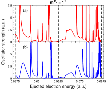
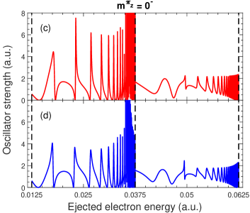
Figure 6: Same as Fig. 4, but with $\gamma=0.025$ a.u.

Note that Wang and Greene Wang expressed caution regarding the reliability of their results at relatively low field strengths. Given the fact that the coupled-channel theory adopts the cylindrical coordinate system, it should be most appropriate for relatively high field strengths. The current results illustrate that this method may approach its limit of validity for magnetic fields around $\gamma=0.01$ a.u. On the contrary, the adiabatic-basis-expansion method was shown to be reliable for low field strengths when comparing its predictions with experimental results at 6.1143 T OMahony . We therefore believe that the spectra for photoionization of magnetized hydrogen atoms at 2,000 T, as calculated in the present work with the adiabatic-basis-expansion method, are more accurate than those from both the coupled-channel theory Zhao2016 and the approach used by Wang and Greene Wang .

IV Summary and conclusions

Since there exist pronounced discrepancies in the predicted positive-energy spectra of atomic hydrogen in a white-dwarf-strength magnetic field obtained by a variety of theoretical approaches reported in the literature, we revisited the problem using the adiabatic-basis-expansion method developed by Mota-Furtado and O’Mahony OMahony2007 , with one significant modification. Specifically, we adopted a different two-dimensional matching procedure to exact the reactance matrix in order to simplify the related calculations. Our test calculations show that such a procedure does not cause any significant numerical inaccuracy.

We then performed a comparative study between the current adiabatic-basis-expansion method and our previously developed coupled-channel theory Zhao2016 . Our calculated positive-energy spectra were also compared to those from other theoretical approaches. A detailed analysis suggests that the adiabatic-basis-expansion method can produce more accurate positive-energy spectra than all the other reported approaches for relatively low field strengths. While we hope that the current study finalizes the problem of photoionization of atomic hydrogen in a white-dwarf-strength magnetic field, we would welcome additional studies from other groups.

References

- (1) R. H. Garstang, Rep. Prog. Phys. 40, 105 (1977).
- (2) W. R. S. Garton and F. S. Tomkins, Astrophys. J. 158, 839 (1969).
- (3) A. Holle, G. Wiebusch, J. Main, B. Hager, H. Rottke, and K. H. Welge, Phys. Rev. Lett. 56, 2594 (1986).
- (4) C. Iu, G. R. Welch, M. M. Kash, D. Kleppner, D. Delande, and J. C. Gay, Phys. Rev. Lett. 66, 145 (1991).
- (5) M. L. Du and J. B. Delos, Phys. Rev. Lett. 58, 1731 (1987); Phys. Rev. A 38, 1896 (1988); Phys. Rev. A 38, 1913 (1988).
- (6) P. F. O’Mahony and F. Mota-Furtado, Phys. Rev. Lett. 67, 2283 (1991).
- (7) S. Watanabe and H. Komine, Phys. Rev. Lett. 67, 3227 (1991).
- (8) L. Ferrario, D. de Martino, and B. T. Gänsicke, Space Sci. Rev. 191, 111 (2015).
- (9) H. Ruder, G. Wunner, H. Herold, and F. Geyer, Atoms in Strong Magnetic Fields: Quantum Mechanical Treatment and Applications in Astrophysics and Quantum Chaos (Springer-Verlag, Berlin, 1994).
- (10) W. Rösner, G. Wunner, H. Herold, and H. Ruder, J. Phys. B 17, 29 (1984).
- (11) H. Forster, W. Strupat, W. Rösner, G. Wunner, H. Ruder, and H. Herold, J. Phys. B 17, 1301 (1984).
- (12) L. B. Zhao and P. C. Stancil, J. Phys. B 40, 4347 (2007).
- (13) L. B. Zhao and F. L. Liu, Mon. Not. R. Astron. Soc. 486, 3849 (2019).
- (14) F. L. Liu and L. B. Zhao, At. Data Nucl. Data Tab. 131, 101285 (2020).
- (15) L. Ferrario, D. Wickramasinghe, A. Kawka, Adv. Space Res. 66, 1025 (2020).
- (16) A. Alijah, J. Hinze and J. T. Broad, J. Phys. B 23, 45 (1990).
- (17) D. Delande, A. Bommier, and J. C. Gay, Phys. Rev. Lett. 66, 141 (1991).
- (18) N. Merani, J. Main and G. Wunner, Astron. Astrophys. 298, 193 (1995).
- (19) L. B. Zhao and P. C. Stancil, Phys. Rev. A 74, 055401 (2006).
- (20) Q. Wang and C. H. Greene, Phys. Rev. A 44, 7448 (1991).
- (21) L. B. Zhao, O. Zatsarinny, and K. Bartschat, Phys. Rev. A 94, 033422 (2016).
- (22) F. Mota-Furtado and P. F. O’Mahony, Phys. Rev. A 76, 053405 (2007).
- (23) M. J. Seaton, Comp. Phys. Commun. 46, 250 (2002).
- (24) E. B. Stechel, R. B. Walker, and J. C. Light, J. Chem. Phys. 69, 3518 (1978).
- (25) M. J. Seaton, Rep. Prog. Phys. 46, 167 (1983).