Object-centered image stitching

Abstract

Image stitching is typically decomposed into three phases: registration, which aligns the source images with a common target image; seam finding, which determines for each target pixel the source image it should come from; and blending, which smooths transitions over the seams. As described in [1], the seam finding phase attempts to place seams between pixels where the transition between source images is not noticeable. Here, we observe that the most problematic failures of this approach occur when objects are cropped, omitted, or duplicated. We therefore take an object-centered approach to the problem, leveraging recent advances in object detection [2, 3, 4]. We penalize candidate solutions with this class of error by modifying the energy function used in the seam finding stage. This produces substantially more realistic stitching results on challenging imagery. In addition, these methods can be used to determine when there is non-recoverable occlusion in the input data, and also suggest a simple evaluation metric that can be used to evaluate the output of stitching algorithms.

1 Image stitching and object detection

Image stitching is the creation of a single composite image from a set of images of the same scene. It is a well-studied problem [5] with many uses in both industry and consumer applications, including Google StreetView, satellite mapping, and the panorama creation software found in modern cameras and smartphones. Despite its ubiquitous applications, image stitching cannot be considered solved. Algorithms frequently produce images that appear obviously unrealistic in the presence of parallax (Figure 1(c)) or object motion (Figure 2(c)), or alternatively indicate that images are too disparate to be stitched when this is not the case. One of the most visually jarring failure modes is the tearing, cropping, deletion, or duplication of recognizable objects. Indeed, it has become a popular internet pastime to post and critique stitching failures of this sort that occur in Google StreetView or on users’ own cameras (most famously, the Google Photos failure shown in Figure 1). In this paper, we exploit advances in object detection [2, 3, 4] to improve image stitching algorithms and avoid producing these artifacts.

The image stitching pipeline typically consists of three phases: registration, in which the images to be stitched are aligned to one another; seam finding, in which a source image is selected for each pixel in the final image; and blending, in which smooths over the transitions between images [5]. In order to avoid introducing object-related errors, we propose modifications to the seam finding step, which typically relies on Markov Random Field (MRF) inference [5, 6]. We demonstrate that MRF inference can be naturally extended to prevent the duplication and maintain the integrity of detected objects. In order to evaluate the efficacy of this approach, we experiment with several object detectors on various sets of images, and show that it can substantially improve the perceived quality of the stitching output when objects are found in the inputs. We also show that object detection algorithms can be used to formalize the evaluation of stitching results, improving on previous evaluation techniques [7] that require knowledge of seam locations.

In the remainder of this section, we give a formal description of the stitching problem, and summarize how our approach fits into this framework. Section 2 gives a short review of related work. In Section 3, we present our object-centered approach for improving seam finding. We propose an object-centered evaluation metric for image stitching algorithms in Section 4. Section 5 gives an experimental evaluation of our techniques, and Section 6 discusses their limitations and possible extensions.

(a) Input images

(b) Our results

(c) Google Photos results

Figure 1: Example showing object cropping. Google Photos (shown) crops the man’s body and blends him into the mountains. APAP [8] and Adobe Photoshop both only include the man’s arm, while NIS [9] produces severe ghosting.

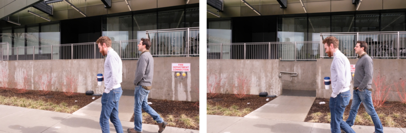
(a) Input images

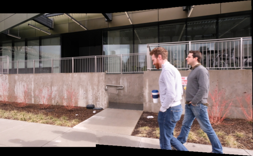
(b) Our results

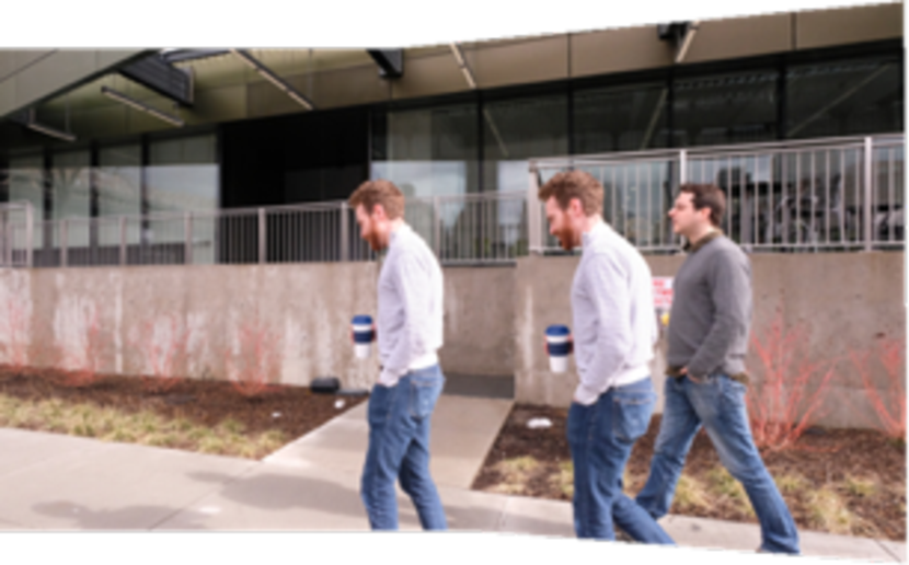
(c) Photoshop results

Figure 2: Example showing object duplication. Photoshop (shown) and APAP give visually similar output, while NIS produces severe ghosting. While we duplicate a shadow on the sidewalk, our object-centered approach preserves the most important elements of the scene.

1.1 Formulating the stitching problem

We use the notation from [10] and formalize the perspective stitching problem as follows: given two images $I_{1},I_{2}$ with an overlap, compute a registration $\omega(I_{2})$ of $I_{2}$ with respect to $I_{1}$, and a label $x_{p}$ for each pixel $p$ that determines whether it gets its value from $I_{1}$ or from $\omega(I_{2})$.

Following [6], the label selection problem is typically solved with an MRF that uses an energy function that prefers short seams with inconspicuous transitions between $I_{1}$ and $\omega(I_{2})$. The energy to be minimized is

$$E(x)=\underset{x\in\mathcal{L}}{\arg\min}\sum_{p}E_{d}(x_{p})\lambda_{d}[M_{i}(p)=0]+\sum_{p,q\in\mathcal{N}}V_{p,q}\cdot[x_{p}\neq x_{q}].$$

The underlying data term $E_{d}$ is combined with a factor $\lambda_{d}[M_{i}(p)=0]$, where $[]$ are Iverson brackets and $M_{i}$ is a mask for each input $i$ that has value 1 if image $I_{i}$ has a value at that location and 0 otherwise. This guarantees that pixels in the output are preferentially drawn from valid regions of the input images.

For a pair of adjacent pixels $p,q\in\mathcal{N}$, the prior term $V_{p,q}$ imposes a penalty for assigning them different labels when the two images have different intensities. A typical choice is $V_{p,q}=|I_{1}(p)-\omega(I_{2})(p)|+|I_{1}(q)-\omega(I_{2})(q)|.$

The generalization to multiple overlapping images is straightforward: with a reference image $I_{1}$ and $k-1$ warped images ${\left\{\omega_{2}(I_{2}),\omega_{3}(I_{3}),\ldots,\omega_{k}(I_{k})\right\}}$, the size of the label set is $k$ instead of $2$ and the worst-case computational complexity goes from polynomial to NP-hard [11]. Despite this theoretical complexity, modern MRF inference methods such as graph cuts are very effective at solving these problems [12].

Our approach. We focus primarily on modifications to the seam finding stage. We introduce three new terms to the traditional energy function that address the cropping, duplication, and occlusion of objects. We also demonstrate that object detection can be used to detect cropping and duplication on the outputs of arbitrary stitching algorithms.

2 Related work

A long-standing problem in image stitching is the presence of visible seams due to effects such as parallax or movement. Traditionally there have been two ways of mitigating these artifacts: to improve registration by increasing the available degrees of freedom [9, 13, 14], or to hide misalignments by selecting better seams. We note that artifacts caused by movement within the scene cannot be concealed by better registration, and that improved seams are the only remedy in these cases.

Our work can be seen as continuing the second line of research. Initial approaches here based the pairwise energy term purely on differences in intensity between the reference image and the warped candidate image [6]. This was later improved upon by considering global structure such as color gradients and the presence of edges[15].

A number of papers make use of semantic information in order to penalize seams that cut through entities that human observers are especially likely to notice, such as faces [16]. One more general approach modifies the energy function based on a saliency measure defined in terms of the location in the output image and human perceptual properties of colors [7]. Our methods differ from these in that we propose general modifications to the energy function that also cleanly handle occlusion and duplication. [17] uses graphcuts to remove pedestrians from Google StreetView images; their technique bears a strong similarity to our duplication term but addresses a different task.

Evaluation of image stitching methods is very difficult, and has been a major roadblock in the past. Most MRF-based stitching methods report the final energy as a measure of quality [6, 12], and therefore cannot be used to compare approaches with different energy functions, or non-MRF based methods. [7] proposes an alternate way to evaluate stitching techniques based on seam quality; their work is perceptually based but similar to MRF energy-based approaches. Our approach, in contrast, takes advantage of more global information provided by object detection.

3 Object-centered seam finding

We use a classic three-stage image stitching pipeline, composed of registration, seam finding, and blending phases. We modify the techniques introduced in [10] to find a single best registration of the candidate image. We then solve a MRF whose energy function incorporates our novel tearing, duplication, and occlusion terms to find seams between the images. Finally, we apply Poisson blending [18] to smooth transitions over stitching boundaries to obtain the final result.

3.1 Registration

Our registration approach largely follows [10], except that we only use a single registration in the seam finding stage. To generate a registration, we first identify a homography that matches a large portion of the image and then run a content-preserving warp (CPW) in order to fix small misalignments [19]. The following provides a high level overview of the registration process.

To create candidate homographies, we run RANSAC on the sparse correspondence between the two input images. In order to limit the set of candidates, homographies that are too different from a similarity transform or too similar to a previously considered one are filtered out at each iteration. The resulting homographies are then refined via CPWs by solving a quadratic program (QP) for each, in which the local terms are populated from the results of an optical flow algorithm run on the reference image and initial candidate registration. This step makes minor non-linear adjustments to the transformation and yields registrations that more closely match portions of the image that would otherwise be slightly misaligned.

We also explored producing multiple registrations and running seam finding on each pair of reference image and candidate registration, and selecting the result by considering both the lowest final energy obtained and the best evaluation score (defined below). This approach is similar to the process used in [14, 20] where homographies are selected based on the final energy from the seam finding phase. We found that this method gave only marginally better results than selecting a single registration.

3.2 Seam finding

The output of the registration stage is a single proposed warp $\omega(I_{2})$. For simplicity, let $I^{S}_{1}=I_{1}$, $I^{S}_{2}=\omega(I_{2})$ be the input images for the seam finding phase. We denote the set of pixels in the output mosaic by $P$. In contrast to the traditional seam finding setup, here we assume an additional input consisting of the results of an object detector run on the input images. We write the set of recognized objects in $I^{S}_{\ell}$ as $O_{\ell}$ and denote by $\mathcal{M}(O_{1},O_{2})\subseteq O_{1}\times O_{2}$ the set of corresponding objects between $O_{1}$ and $O_{2}$. The computation of $\mathcal{M}(O_{1},O_{2})$ is discussed in Section 3.5.

Besides $I^{S}_{1}$ and $I^{S}_{2}$, we use an additional label $\bot$, indicating that no value is available for that pixel due to occlusion. The label set for the MRF is then $\mathcal{L}=\{\bot,1,2\}$, where $x_{p}=1$ or $x_{p}=2$ indicate that the pixel is copied from $I^{S}_{1}$ or $I^{S}_{2}$, and a label of $x_{p}=\bot$ indicates that the pixel is occluded by an object in all input images and therefore cannot be accurately reproduced.

Given this MRF, we solve for a labeling $x$ using an objective function that, in addition to the traditional data and smoothness terms $E_{d}$ and $E_{s}$, contains three new terms that we introduce here: a cropping term $E_{c}$, a duplication term $E_{r}$, and an occlusion term $E_{o}$, which are presented in Section 3.3, following a brief review of the traditional terms. Using a 4-connected adjacency system $\mathcal{N}$ and tradeoff coefficients $\lambda_{d},\lambda_{s},\lambda_{c},\lambda_{r},\lambda_{o},\delta$, the final energy is then given by:

$$E(x)= \lambda_{d}\sum_{p\in P}E_{d}(x_{p})+\lambda_{s}\sum_{p,q\in\mathcal{N}}E_{s}(x_{p},x_{q}) + \lambda_{c}\sum_{\ell\in\mathcal{L}}\sum_{o\in O_{\ell}}E_{c}(x;o,\ell)\ +$$ (1)

$$\lambda_{r}\!\!\!\!\!\!\!\!\sum_{(o_{1},o_{2})\in\mathcal{M}(O_{1},O_{2})}\!\!\!\!\!\!\!\!E_{r}(x;o_{1},o_{2}) + \lambda_{o}\!\!\!\!\!\!\!\!\sum_{(o_{1},o_{2})\in\mathcal{M}(O_{1},O_{2})}E_{o}(x;o_{1},o_{2})$$

3.2.1 Data term $E_{d}(x_{p})$

This term is given by

$$E_{d}(x_{p})=\begin{cases}0,&\qquad x_{p}\neq\bot\wedge M_{x_{p}}(p)=1,\\ 1,&\qquad x_{p}\neq\bot\wedge M_{x_{p}}(p)=0,\\ 1+\delta,&\qquad x_{p}=\bot\end{cases}$$

This term penalizes choosing a pixel in the output from an input image $i$ if the pixel is not in the mask ($M_{i}(p)=0$), or for declaring a pixel occluded. The $\delta$ parameter determines how strongly we prefer to leave a pixel empty rather than label it as occluded, and is discussed further in the definition of the occlusion term $E_{o}$ below. There is no preference between the two source images.

3.2.2 Smoothness term $E_{s}(x_{p},x_{q})$

To define this term we need the following notation: $\mathcal{C}(p,q,r)=\{k\mid\min(\|k-p\|_{1},\|k-q\|_{1})\leq r\}$ is the set of pixels within L1 distance $r$ of either pixel $p$ or $q$, describing a local patch around adjacent pixel $p$ and $q$, while $I_{max}=\max_{p,q}\sum_{k\in\mathcal{C}(p,q,r)}\|I_{1}^{S}(k)-I_{2}^{S}(k)\|$. Writing exclusive-or as $\oplus$, our smoothness term is

$$E_{s}(x_{p},x_{q})=\begin{cases}0,&\qquad x_{p}=x_{q},\\ I_{max},&\qquad x_{p}=\bot\oplus x_{q}=\bot,\\ \sum_{k\in\mathcal{C}(p,q,r)}\|I^{S}_{x_{p}}(k)-I^{S}_{x_{q}}(k)\|,&\qquad\text{else}.\\ \end{cases}$$

Note that our term for the case $x_{p}=\bot\oplus x_{q}=\bot$ discourages the MRF from transitioning into the occluded label.

In general, $E_{s}$ penalizes the local photometric difference for a seam between pixels $p$ and $q$ when $x_{p}\neq x_{q}$. In the special case where $r=0$, $\mathcal{C}(p,q,r)=\{p,q\}$, and the cost of the seam here is $\lambda_{s}(\|I^{S}_{x_{p}}(p)-I^{S}_{x_{q}}(p)\|+\|I^{S}_{x_{p}}(q)-I^{S}_{x_{q}}(q)\|)$ as in most seam finding algorithms. Values of $r>0$ will lead to larger local patches.

3.3 Our new MRF terms

3.3.1 Cropping term $E_{c}$

We introduce a term that penalizes seams that cut through an object $o\in O_{\ell}$, with cost proportional to the length of the seam.

$E_{c}(x;o,\ell)=\sum_{p\in o}\sum_{q\in o}[x_{p}=\ell,x_{q}\neq\ell]$

The value of this term is $0$ exactly when object $o$ is either drawn entirely from $I^{S}_{\ell}$, or not present at all in the final stitching result ($x_{p}=\ell,\forall p\in o$ or $x_{p}\neq\ell,\forall p\in o$, respectively). As defined, this results in $|o|^{2}$ pairwise terms, which may cause the optimization to be intractable in practice. As a result, we use an approximation of this term in the experiments, discussed in 3.4.

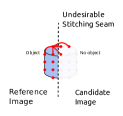
(a)

(b)

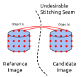
(c)

(d)

Figure 3: Figure 3(a) depicts our crop term. We use pairwise terms to penalize any seam that cuts through an object. Figure 3(b) depicts a crop error created by Photoshop. Figure 3(c) depicts our duplication term. We use pairwise terms to penalize any seam that results in the same object appearing in two different locations on the final mosaic. Figure 3(d) depicts a duplication error created by NIS.

Note that since this term is a penalty rather than a hard constraint, the tradeoff between the smoothness term $E_{s}$ and this term $E_{c}$ will still allow us to cut through an object if it sufficiently benefits photometric consistency.

3.3.2 Duplication term $E_{r}$

Our term discourages duplication when $o_{1}$ in $I^{S}_{1}$ and $o_{2}$ in $I^{S}_{2}$ are known to refer to the same object, and is defined as

$E_{r}(x;o_{1},o_{2})=\sum_{(p,q)\in m(o_{1},o_{2})}[x_{p}=1\land x_{q}=2].$

Here $m(o_{1},o_{2})\in o_{1}\times o_{2}$ are the pixel-level correspondences between objects $o_{1}$ and $o_{2}$. $(p,q)\in m(o_{1},o_{2})$ represent the same point in the real world, so the final stitching result should not include both pixel $p$ from $o_{1}$ and pixel $q$ from $o_{2}$. Note that this term includes a potentially complicated function $m$ that calculates dense pixel correspondences; as a result, we use an approximation of this term in the experiments, discussed in 3.4.

3.3.3 Occlusion term $E_{o}$

This term promotes the occlusion label by penalizing the use of out-of-mask labels in areas of the image where duplicate objects were detected:

$$\begin{split}E_{o}(x;o_{1},o_{2})=2\delta\sum_{\ell\in\{1,2\}}\sum_{p\in o_{\ell}}[M_{\ell}(p)=0\land x_{p}=\ell]\end{split}$$ (2)

where $\delta$ is the same parameter used to penalize the selection of the $\bot$ label in $E_{d}$. For the intuition behind this term, consider the case where $o_{1}$ and $o_{2}$ are corresponding objects in $I^{S}_{1}$ and $I^{S}_{2}$, and $M_{2}(p)=0$ for $p\in o_{1}$. Then we must either select label $1$ for the pixels in $o_{1}$ or declare the pixels occluded. The data term $E_{d}$ ensures that the occlusion label will normally give higher energy than a label which is out of mask. However, in the presence of a duplicated object, the occlusion term $E_{o}$ increases the energy of the out of mask term since $2\delta>\delta$, resulting in the occlusion label being selected instead. Note, we typically set $\lambda_{o}=\lambda_{d}$.

3.3.4 Generalization to 3 or more images.

With multiple inputs, one image acts as the reference and the others become candidates. We then calculate registrations in the same manner as before, then pass to the seam finding phase the reference image and the candidate registrations: $I_{1}$ and $\omega_{2}(I_{2}),\ldots,\omega_{n}(I_{n})$. We calculate correspondence for all pairs of images. When establishing correspondence between objects, we make sure that correspondence acts as an equivalence relation. The primary difference between the two and three input image case is transitivity. If three objects violate transitivity, we increase the correspondence threshold until the property holds. While other schemes could be imagined to ensure consistency, experimentally, we have yet to see this be violated.

3.4 Optimization

The cropping term $E_{c}$ above has dense connections between each pixel $p\in I^{S}_{1}$ and $q\in I^{S}_{2}$, which can lead to computational difficulties. Here we introduce a local energy term $E_{lc}$ that has fewer connections and is therefore simpler to compute, while experimentally maintaining the properties of the terms introduced above:

$$E_{lc}(x;o,\ell)=\sum_{p\in o}\sum_{q\in N_{p}}[x_{p}=\ell,x_{q}\neq\ell]$$

where $N_{p}$ is set of neighbors for $p$.

Similarly, the duplication term reported above has a complicated structure based on the matching function over detected objects. We define the local duplication term $E_{lr}$ in terms of $m_{b}(o_{1},o_{2})$, which in contrast to $m(o_{1},o_{2})$, returns the corresponding points of the two bounding boxes around objects $o_{1}$ and $o_{2}$, where each $p\in o_{1}$ is bilinearly interpolated to its position in $o_{2}$ using the corners of the bounding box.

To solve this MRF, we use alpha-expansion [11] with QPBO [21] for the induced binary subproblems. QPBO has been reported to perform well on a variety of computer vision tasks in practice, even when the induced binary subproblem is supermodular [21].

3.5 Establishing correspondence between objects

Our strategy is to consider pairs of objects $o_{1},o_{2}$ detected in images $I_{1}$, $\omega(I_{2})$ respectively and to compute a metric that represents our degree of confidence in their corresponding to the same object. We compute this metric for all object pairs over all images and declare the best-scoring potential correspondence to be a match if it exceeds a specified threshold. In addition to the correspondence density metric used in the experiments reported here, we considered and tested several different metrics that we also summarize below. In all cases, the category returned by the object detector was used to filter the set of potential matches to only those in the same category.

Feature point matching. We tried running SIFT [22] and DeepMatch [23] directly on the objects identified. These methods gave a large number of correspondences without spatial coherence; for example, comparing a car and bike would result in a reasonable number of matches but the points in image $I_{1}$ would match to points very far away in $I_{2}$. We tried to produce a metric that captured this by comparing vector difference between feature points $p$ and $q$ from $I_{1}$ to their correspondences $p^{\prime}$ and $q^{\prime}$ from $I_{2}$.

Correspondence density. We ran DeepMatch [23] on the two input images and counted the matches belonging to the two objects being considered as a match. This number was then divided by the area of the first image. Since DeepMatch feature points are roughly uniformly distributed in the first input image, the density of points in the area of the first input has an upper bound and it is possible to pick a density threshold that is able to distinguish between matching and non-matching objects, regardless of their size. This is the technique used in the experimental section below.

4 Object-centered evaluation of stitching algorithms

We now discuss the use of object detectors for formalized evaluation of stitching algorithms. In general, we assume access to the input images and the final output. The available object detectors are run on both, and their output used to identify crops, duplication, or omissions introduced by the stitching algorithm. The goal of this evaluation technique is not to quantify pixel-level discontinuities, e.g. slight errors in registration or seam-finding, but rather to determine whether the high-level features of the scene, as indicated by the presence and general integrity of the objects, are preserved.

In the following, $F$ denotes the final output panorama, $I$ the set of input images, and $N_{X}$ the number of objects detected in an image $X$. $N_{F}$, for instance, would denote the number of objects found by a detector in the stitch result. Note that the techniques we propose can also be applied in parallel for specific categories of objects: instead of a general $O$ and $N_{F}$, we might consider $O^{c}$ and $N_{F}^{c}$ for a particular category of objects $c$, e.g. humans or cats. Separating the consideration of objects in this way makes object analysis more granular and more likely to identify problems with the scene.

4.1 Penalizing omission and duplication

We first attempt to evaluate the quality of a stitch through the number of objects $N$ detected in the input images and the final output. We generalize $\mathcal{M}(O_{1},\ldots,O_{n})$ to apply to an arbitrary number of input images, denoting corresponding object detections across a set of images $I_{1},\ldots,I_{n}$. The techniques discussed above for establishing correspondences between objects can easily be generalized to multiple images and used to formulate an expression for the expected number of objects in the final stitch result. In particular, the expected object count for a hypothetical ideal output image $F^{*}$ is given by the number of “equivalence classes” of objects found in the input images for the correspondence function under consideration: all detected objects are expected to be represented at least once, and corresponding objects are expected to be represented with a single instance.

For a good stitching output $F$, we expect $N_{F}=N_{F^{*}}$. Note that $N_{F}>N_{F^{*}}$ or $N_{F}<N_{F^{*}}$ imply omissions or duplications, respectively. In Figure 4, a human detector finds objects in only one image and $\mathcal{M}(O_{1},O_{2})=\emptyset$; therefore, we have that $N_{F^{*}}=2$ for the category of humans. When run on the output of Photoshop or APAP, however, only one human is found, giving $N_{F}<N_{F^{\prime}}$ and indicating an omission.

Other approaches exist for detecting omission or duplication that do not require computing the potentially complicated $\mathcal{M}$ function. For example, it can be inferred that an object has been omitted in the output if it contains fewer objects than any of the inputs: $N_{F}<\max_{I_{i}\in I}(|O_{i}|)$. Similarly, a duplication has occurred if more objects are identified in the output than the total number of objects detected in all of the input images: $N_{F}>\sum_{I_{i}\in I}N_{I_{i}}$. While this may seem to be a weak form of inference, it proves sufficient in Figure 4: the maximum number of humans in an input image is $2$, but only one is found in the Photoshop and APAP results, indicating an omission.

Unfortunately, while duplication almost always indicates an error in an output $F$, the situation is not as clear-cut with omissions. Objects that are not central to the scene or that are not considered important by humans for whatever reason can often be omitted without any negative effect on the final mosaic.

4.2 Cropping

(a) Input image

(b) Google Photos (0.1140)

(c) Photoshop (no object)

(d) APAP (0.1203)

(e) Our result (left 0.4882, right 0.93380)

Figure 4: Visualizations for object bounding boxes for humans detected in given source. Final mosaics have been altered for space reasons, but no bounding boxes were removed. The MS-SSIM are listed in parenthesis after the method name. $N_{F}-N_{F^{*}}$ is as follows (b) -1, (c) -2, (d) -1, and (e) 0.

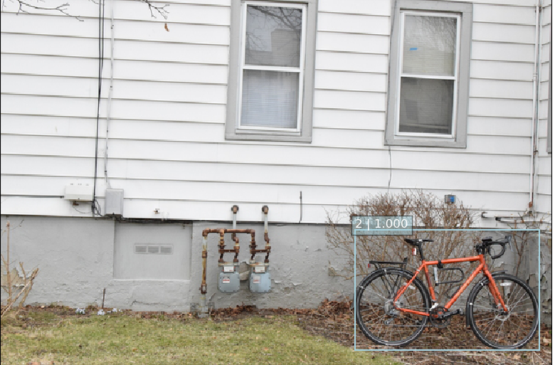
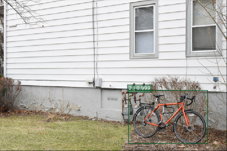
(a) Input images

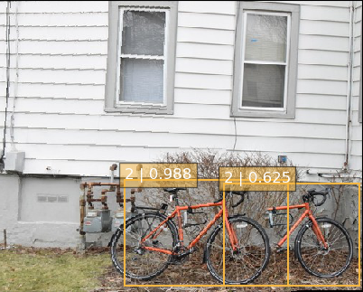
(b) APAP

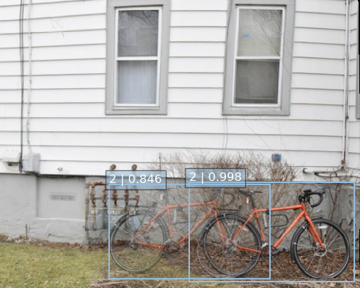
(c) NIS

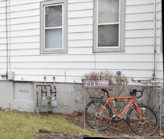
(d) Our result

Figure 5: Visualizations for object bounding boxes for bikes detected in given source. Final mosaics have been altered for space reasons, but no bounding boxes were removed. Other techniques failed to produce a stitch. The MS_SSIM are as follows: APAP left (0.1608), APAP right (0.1523), NIS left (0.3971), NIS right (0.1771), Ours (0.8965). $N_{F}-N_{F^{*}}$ is as follows (b) 1, (c) 1, and (d) 0

(a) Input image

(b) Autostitch (0.4575)

(c) NIS (0.5201)

(d) Photoshop (0.5099)

(e) APAP (0.4773)

(f) Our result (0.6769)

Figure 6: Object bounding boxes for cats detected in given source. MS_SSIM is included in parenthesis. Autostitch applies a warp that alters the cat’s facial shape. NIS contains ghosting. Photoshop duplicates part of the cat’s face. APAP applies a warp that alters the cat’s facial shape.

Object detectors can be used to detect crops in two ways: major crops, which make the object unrecognizable to the detector, are interpreted by our system as omissions, and detected as described above. Even objects that are identifiable in the final output, however, may be partially removed by a seam that cuts through them or undergo unnatural warping. A different approach is therefore needed in order to detect and penalize these cases. Here we consider two options that differ in whether they consider the results of the object detector on the input images: the first directly compares the detected objects from the inputs and output, while the second is less sensitive to the choice of object detector and instead uses more generic template matching methods.

For both of the methods, we note that some warping of the input image is usually necessary in order to obtain a good alignment, so image comparison techniques applied to the original input image and the output image are unlikely to be informative. However, given an input image $I_{i}$ and the output $F$ it is possible to retrospectively compute a set of plausible warps $\omega(I_{i})$ and apply image comparison operators to these. Our approach therefore does not require access to the actual warp used to construct the stitch, but it can of course be used to increase the accuracy of our methods if it is available.

Cropping detection with direct object comparison. This approach implicitly trusts the object detector to give precise results on both the input images and the output image. The object detector is run for $F$ and for all of the plausible registration candidates that have been determined for the various $I_{i}$. We then run Multiscale Structural Similarity (MS-SSIM) [24] for all of the correspondences among the detected objects (determined as discussed in Section 3.5), and use the average and maximum values of these metrics as our final result. Any reasonable image similarity metric can be used in this approach, including e.g. deep learning techniques.

Cropping detection with template matching. This metric is less sensitive to the choice of object detector. Instead of applying it to all of the warped input images, we apply it only to the result image. The region of the output where the object is detected is then treated as a template, and traditional template matching approaches are used to compare the object to the reference image $I_{1}$ and any plausible registrations.

We have experimented with these metrics to confirm that these values match our intuitions about the handling of objects in the stitch result. We provide some examples and their evaluation values (maximum MS-SSIM with direct object comparison) in the captions of the figures above.

5 Experimental results for stitching

Our goal is to stitch difficult image sets that give rise to noticeable errors with existing approaches. Unfortunately, there is no standard data set of challenging stitching problems, nor any generally accepted metric to use other than subjective visual evaluation. We therefore follow the experimental setup of [20], who both introduce a stitching technique that is able to stitch a difficult class of images, and also present a set of images that cause previous methods to introduce duplications and cropping. For competitors we consider Photoshop 2018’s “Photomerge” stitcher, APAP [8], Autostitch [25], and NIS[9]. Following the approach of [20], we extend APAP with a seam finder.

Experimental Setup. We tried several methods for feature extraction and matching, and found that DeepMatch [23] gave the best results. It was used in all examples shown here. The associated DeepFlow solver was used to generate flows for the optical flow-based warping. The QP problems used to obtain the mesh parameters and determine candidate warpings $\omega_{i}$ were solved with the Ceres solver [26]. For object detection, we experimented with the Mask R-CNN [4] and SSD [3] systems. Both were found to give good performance for different types of objects.

Ablation Study. We performed an ablation study on the pairwise terms in the seam finding stage and found that all terms are necessary and perform as expected. These results are available with the rest of the data as indicated below.

In the remainder of this section, we review several images from our test set and highlight the strengths and weaknesses of our technique, as well as those of various methods from the literature. All results shown use the same parameter set. Data, images and additional material omitted here due to lack of space are available online.

(a) Inputs

(b) Photoshop result

(c) Our result

Figure 7: “Bottle” dataset. Photoshop duplicates the neck of the bottle and the headphones. Our result is plausible.

(a) Inputs

(b) Photoshop result

(c) Our result

Figure 8: “Walking” dataset.

(a) Inputs

(b) Photoshop result

(c) Our result

Figure 9: “Pet Store” dataset. Photoshop omits the left arm. Our result is plausible.

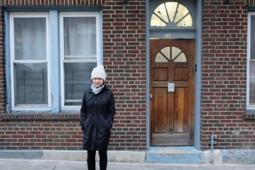
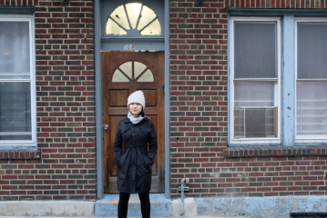
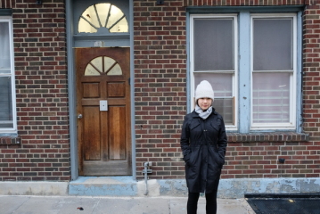
(a) Candidate and reference images

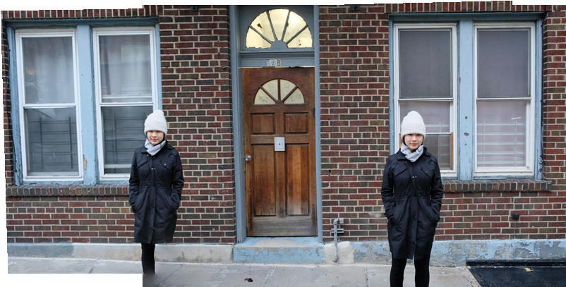
(b) Photoshop result

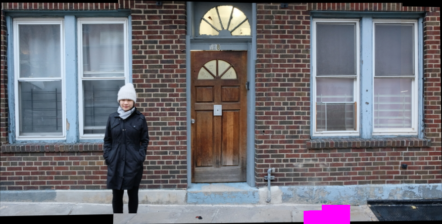
(c) Our result with occlusion detected

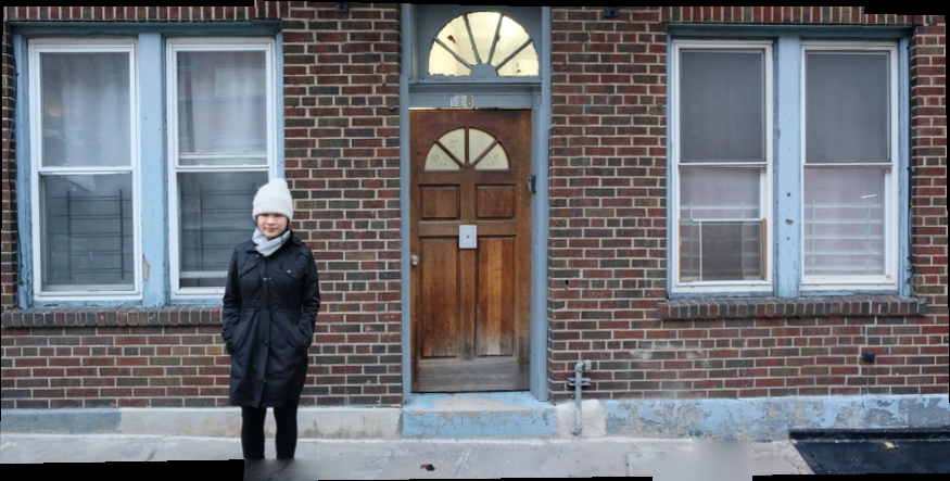
(d) Our blend result

(e) Our cropped result

Figure 10: Three image stitching. In 10(c), we choose to not use the human in the right-most input. However, the legs block any information regarding the sidewalk, making this location occluded. Our algorithm correctly labels it as occluded and colors it magenta. 10(d) and 10(e) present ways to fix this occlusion.

6 Conclusions, limitations and future work

We have demonstrated that object detectors can be used to avoid a large class of visually jarring image stitching errors. Our techniques lead to more realistic and visually pleasing outputs, even in hard problems with perspective changes and differences in object motion, and avoid artifacts such as object duplication, cropping, and omission that arise with other approaches. Additionally, object detectors yield ways of evaluating the output of stitching algorithms without any dependence on the methods used.

One potential drawback to our approach is that it applies only to inputs containing detectable objects, and provides no benefit in e.g. natural scenes where current object detection techniques are unable to generate accurate bounding boxes for elements such as mountains or rivers. We expect, however, that our techniques will become increasingly useful as object detection and scene matching improve. At the other end of the spectrum, we may be unable to find a seam in inputs with a large number of detected objects. We note that our crop, duplication, and omission terms are all soft constraints. In addition, objects can be prioritized based on saliency measures or category (i.e. human vs. other), and crops penalized more highly for objects deemed important. One existing use case where this might apply is for city imagery with pedestrians moving on sidewalks, such as the content of Google Streetview. Traditional seam finding techniques find this setting particularly difficult, and torn or duplicated humans are easily identifiable errors.

False positives from object correspondences are another issue. In this case, matching thresholds can be adjusted to obtain the desired behavior for the particular use case. Scenes with a large number of identical objects, such as traffic cones or similar cars, present a challenge when correspondence techniques are unable to match the objects to one another by taking advantage of the spatial characteristics of the input images. One issue that our technique cannot account for is identical objects with different motions: a pathological example might be pictures of identically-posed twins wearing the same clothing. We consider these false positives to be a reasonable tradeoff for improved performance in the more common use case.

6.0.1 Acknowledgements.

This research has been supported by NSF grants IIS-1161860 and IIS-1447473 and by a Google Faculty Research Award. We also thank Connie Choi for help collecting images.

References

- [1] Szeliski, R.: Image alignment and stitching: A tutorial. Foundations and Trends in Computer Graphics and Vision 2(1) (2007) 1–104
- [2] Goodfellow, I., Bengio, Y., Courville, A.: Deep Learning. The MIT Press (2016)
- [3] Liu, W., Anguelov, D., Erhan, D., Szegedy, C., Reed, S., Fu, C.Y., Berg, A.C.: SSD: Single shot multibox detector. In: ECCV, Springer (2016) 21–37
- [4] Ren, S., He, K., Girshick, R., Sun, J.: Faster R-CNN: Towards real-time object detection with region proposal networks. TPAMI 39(6) (2017) 1137–1149
- [5] Szeliski, R.: Computer Vision: Algorithms and Applications. Springer (2010)
- [6] Kwatra, V., Schödl, A., Essa, I., Turk, G., Bobick, A.: Graphcut textures: Image and video synthesis using graph cuts. SIGGRAPH 22(3) (2003) 277–286
- [7] Li, N., Liao, T., Wang, C.: Perception-based seam cutting for image stitching. Signal, Image and Video Processing (2018)
- [8] Zaragoza, J., Chin, T.J., Brown, M.S., Suter, D.: As-projective-as-possible image stitching with moving dlt. In: CVPR. (2013) 2339–2346
- [9] Chen, Y.S., Chuang, Y.Y.: Natural image stitching with the global similarity prior. In: ECCV. (2016) 186–201
- [10] Herrmann, C., Wang, C., Bowen, R.S., Keyder, E., Krainin, M., Liu, C., Zabih, R.: Robust image stitching using multiple registrations. In: ECCV. (2018)
- [11] Boykov, Y., Veksler, O., Zabih, R.: Fast approximate energy minimization via graph cuts. TPAMI 23(11) (2001) 1222–1239
- [12] Szeliski, R., Zabih, R., Scharstein, D., Veksler, O., Kolmogorov, V., Agarwala, A., Tappen, M., Rother, C.: A comparative study of energy minimization methods for Markov Random Fields. TPAMI 30(6) (2008) 1068–1080
- [13] Lin, C.C., Pankanti, S.U., Natesan Ramamurthy, K., Aravkin, A.Y.: Adaptive as-natural-as-possible image stitching. In: CVPR. (2015) 1155–1163
- [14] Lin, K., Jiang, N., Cheong, L.F., Do, M., Lu, J.: Seagull: Seam-guided local alignment for parallax-tolerant image stitching. In: ECCV. (2016) 370–385
- [15] Agarwala, A., Dontcheva, M., Agrawala, M., Drucker, S., Colburn, A., Curless, B., Salesin, D., Cohen, M.: Interactive digital photomontage. SIGGRAPH 23(3) (2004) 294–302
- [16] Ozawa, T., Kitani, K.M., Koike, H.: Human-centric panoramic imaging stitching. In: Augmented Human International Conference. (2012) 20:1–20:6
- [17] Flores, A., Belongie, S.: Removing pedestrians from google street view images. In: IEEE International Workshop on Mobile Vision. (2010) 53–58
- [18] Perez, P., Gangnet, M., Blake, A.: Poisson image editing. SIGGRAPH (2003) 313–318
- [19] Liu, F., Gleicher, M., Jin, H., Agarwala, A.: Content-preserving warps for 3D video stabilization. SIGGRAPH 28(3) (2009)
- [20] Zhang, F., Liu, F.: Parallax-tolerant image stitching. In: CVPR. (2014) 3262–3269
- [21] Kolmogorov, V., Rother, C.: Minimizing nonsubmodular functions with graph cuts-a review. TPAMI 29(7) (2007) 1274–1279
- [22] Lowe, D.: Object recognition from local scale-invariant features. In: ICCV. (1999) 1150–1157
- [23] Weinzaepfel, P., Revaud, J., Harchaoui, Z., Schmid, C.: Deepflow: Large displacement optical flow with deep matching. In: ICCV. (2013) 1385–1392
- [24] Wang, Z., Simoncelli, E., Bovik, A.: Multiscale structural similarity for image quality assessment. In: Asilomar Conference on Signals, Systems and Computers. (2004) 1398–1402
- [25] Brown, M., Lowe, D.G.: Automatic panoramic image stitching using invariant features. IJCV 74(1) (2007) 59–73
- [26] Agarwal, S., Mierle, K., Others: Ceres solver. http://ceres-solver.org. Accessed: 2018-07-25.