Robust image stitching with multiple registrations

Abstract

Panorama creation is one of the most widely deployed techniques in computer vision. In addition to industry applications such as Google Street View, it is also used by millions of consumers in smartphones and other cameras. Traditionally, the problem is decomposed into three phases: registration, which picks a single transformation of each source image to align it to the other inputs, seam finding, which selects a source image for each pixel in the final result, and blending, which fixes minor visual artifacts [1, 2]. Here, we observe that the use of a single registration often leads to errors, especially in scenes with significant depth variation or object motion. We propose instead the use of multiple registrations, permitting regions of the image at different depths to be captured with greater accuracy. MRF inference techniques naturally extend to seam finding over multiple registrations, and we show here that their energy functions can be readily modified with new terms that discourage duplication and tearing, common problems that are exacerbated by the use of multiple registrations. Our techniques are closely related to layer-based stereo [3, 4], and move image stitching closer to explicit scene modeling. Experimental evidence demonstrates that our techniques often generate significantly better panoramas when there is substantial motion or parallax.

1 Image stitching and parallax errors

The problem of image stitching, or the creation of a panorama from a set of overlapping images, is a well-studied topic with widespread applications [5, 6, 7]. Most modern digital cameras include a panorama creation mode, as do iPhones and Android smartphones. Google Street View presents the user with panoramas stitched together from images taken from moving vehicles, and the overhead views shown in map applications from Google and Microsoft are likewise stitched together from satellite images. Despite this ubiquity, stitching is far from solved. In particular, stitching algorithms often produce parallax errors even in a static scene with objects at different depths, or dynamic scene with moving objects. An example of motion errors is shown in Figure 1.

(a) Input images

(b) Our result

(c) Autostitch [8]

Figure 1: Motion errors example. The strip of papers with numbers has undergone translation between input images. Our result in 1(b) shows the use of multiple registrations. Green: the reference, Red: registration aligning the number strip, Blue: registration aligning the letter strip. Autostitch result in 1(c) has visible ghosting on the number strip.

The stitching problem is traditionally viewed as a sequence of steps that are optimized independently [6, 7]. In the first step, the algorithm computes a single registration for each input image to align them to a common surface. The warped images are then passed on to the seam finding step; here the algorithm determines the registered image it should draw each pixel from. Finally, a blending procedure [9] is run on the composite image to correct visually unpleasant artifacts such as minor misalignment, or differences in color or brightness due to different exposure or other camera characteristics.

In this paper, we argue that currently existing methods cannot capture the required perspective changes for scenes with parallax or motion in a single registration, and that seam finding cannot compensate for this when the seam must pass through content-rich regions. Single registrations fundamentally fail to capture the background and foreground of a scene simultaneously. This is demonstrated in Figure 1, where registering the background causes errors in the foreground and vice versa. Several papers [1, 2] have addressed this problem by creating a single registration that is designed to produce a high quality stitch. However, as we will show, these still fail in cases of large motion or parallax due to the limitations inherent to single registrations. We instead propose an end-to-end approach where multiple candidate registrations are presented to the seam finding phase as alternate source images. The seam finding stage is then free to choose different registrations for different regions of the composite output image. Note that as any registration can serve as a candidate under our scheme, it represents a generalization of methods that attempt to find a single good registration for stitching.

Unfortunately, the classical seam finding approach [5] does not naturally work when given multiple registrations. First, traditional seam finding treats each pixel from the warped image equally. However, by the nature of our multiple registration algorithm, each of them only provides a good alignment for a particular region in the image. Therefore, we need to consider this pixel-level alignment quality in the seam finding phase. Second, seam finding is performed locally by setting up an MRF that tries to place seams where they are not visually obvious. Figure 1 illustrates a common failure; the best seam can cause objects to be duplicated. This issue is made worse by the use of multiple registrations. In traditional image stitching, pixels come from one of two images, so in the worst case scenario, an object is repeated twice. However, if we use $n$ registrations, an object can be repeated as many as $n+1$ times.

We address this issue by adding several additional terms to the MRF that penalize common stitching errors and encourage image accuracy. Our confidence term encourages pixels to select their value from registrations which align nearby pixels, our duplication term penalizes label sets which select the same object in different locations from different input images, and finally our tear term penalizes breaking coherent regions. While our terms are designed to handle the challenges of multiple registrations, they also provide improvements to the classical single-registration framework.

Our work can be interpreted as a layer-based approach to image stitching, where each registration is treated as a layer and the seam finding stage simultaneously solves for layer assignment and image stitching [3]. Under this view, this paper represents a modest step towards explicit scene modeling in image stitching.

1.1 Motivating examples

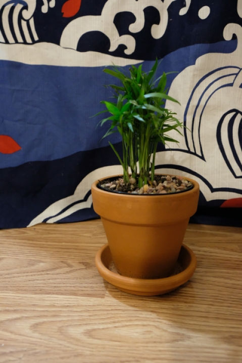
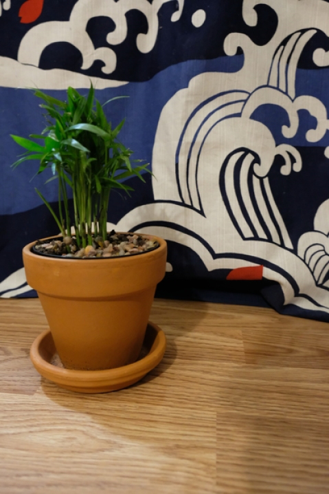
(a) Input images

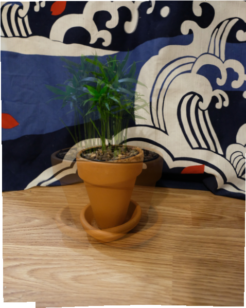
(b) NIS [10]

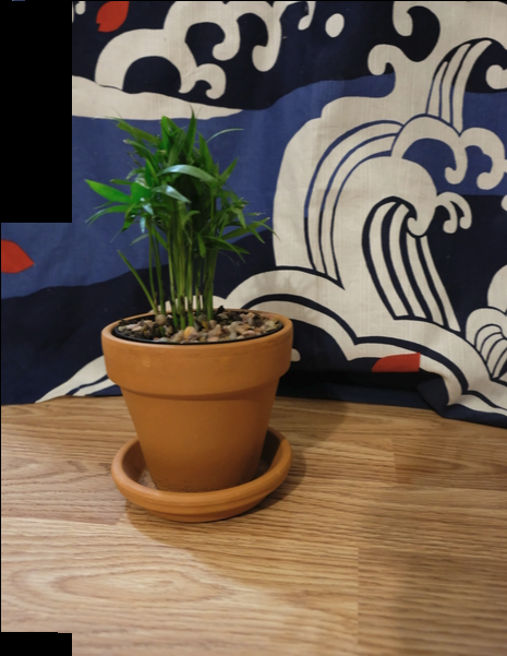
(c) Our result

Figure 2: Motivating example for multiple registrations. Even the sophisticated single registration approach of NIS [10] gives severe ghosting.

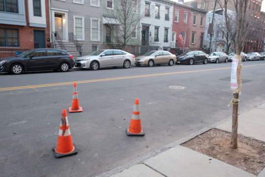
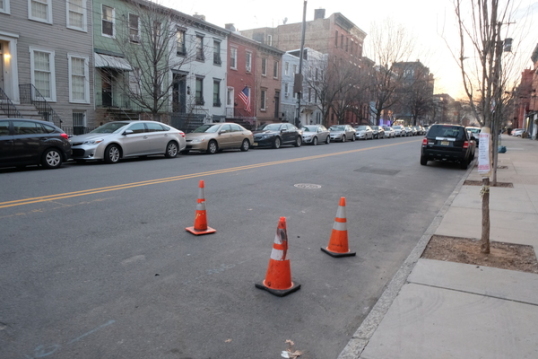
(d) Input images

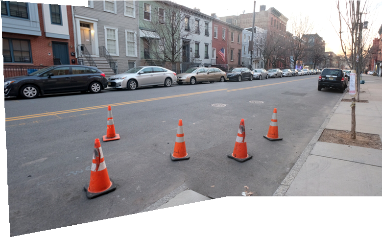
(e) Photoshop [11]

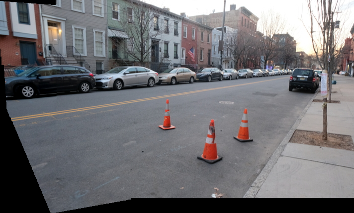
(f) Our result

Figure 3: Motivating example for multiple registrations. State of the art commercial packages like Adobe Photoshop [11] duplicate the traffic cones and other objects.

Figure 3 demonstrates the power of multiple registrations. The plant, the floor and the wall each undergo very distinctive motions. Our technique captures all 3 motions. Another challenging example is shown in Figure 3. Photoshop computes a single registration to align the background buildings, which duplicates the traffic cones and the third car from left. Our technique handles all these objects at different depth correctly.

1.2 Problem formulation and our approach

We adopt the common formulation of image stitching, sometimes called perspective stitching [12] or a flat panorama [6, §6.1], that takes one image $I_{0}$ as the reference, then warps another candidate image $I_{1}$ into the reference coordinate system, and add its content to $I_{0}$.

Instead of proposing a single warped $\omega(I_{1})$ and sending it to the seam finding phase, we proposed a set of warping $\omega_{1}(I_{1}),\ldots,\omega_{N}(I_{1})$, where each $\omega_{i}(I_{1})$ aligns a region in $I_{1}$ with $I_{0}$. We will detail our approach for multiple registrations in Section 3.1. Then we will formalize a multi-label MRF problem for seam finding. We have label set $\mathcal{L}=\{0,1,\ldots,N\}$, such that label $x_{p}=0$ indicates pixel $p$ in the final stitched result will take its color value from $I_{0}$, and from $\omega_{x_{p}}(I_{1})$ when $x_{p}>0$. We will get the optimal seam by minimizing the energy function $E(x)$ with the new proposed terms to address the challenges we introduced before. We will describe our seam finding energy $E(x)$ in Section 3.2. Finally, we adopt Poisson blending [9] to smooth transitions over stitching boundaries when generating the final result.

2 Related work

The presence of visible seams due to parallax and other effects is a long-standing problem in image stitching. Traditionally there have been two avenues for eliminating or reducing these artifacts: improving registrations by allowing more degrees of freedom, or hiding misalignments by selecting better seams. Our algorithm can be seen as employing both of these strategies: the use of multiple registrations allows us to better tailor each registration to a particular region of the panorama, while our new energy terms improve the quality of the final seams.

2.1 Registration

Most previous works take a homography as a starting point and perform additional warping to correct any remaining misalignment. [13] describes a process in which each feature is shifted toward the average location of its matches in other images. The APAP algorithm divides images into grid cells and estimates a separate homography for each cell, with regularization toward a global homography [14].

Instead of solving registration and seam finding independently, another line of work explicitly takes into account the fact that the eventual goal of the registration step is to produce images that can be easily stitched together. ANAP, for instance, can be improved by limiting perspective distortions in regions without overlap and otherwise regularizing to produce more natural-looking mosaics [15]. Another approach is to confine the warping to a minimal region of the input images that is nevertheless large enough for seam selection and blending, which allows the algorithm to handle larger amounts of parallax [2]. Going a step further it is possible to interleave the registration and seam finding phases, as in the SEAGULL system [1]. In this case, the mesh-based warp can be modified to optimize feature correspondences that lie close to the current seam.

2.2 Seam finding and other combination techniques

The seam finding phase requires determining, for each pixel, which of the two source images contributes its color. [5] observed that this problem can be naturally formulated as a Markov Random Field and solved via graph cuts. This approach tends to give strong results, and the graph cuts method in particular often produces energies that are within a few percent of the global minimum [16]. Further work in this area has focused on taking into account the presence of edges or color gradients in the energy function in order to avoid visible discontinuities. [17].

An alternative to seam finding is the use of a a multi-band blending [18] phase immediately after registration [8]. This step blends low frequencies over a large spatial range and high frequencies over a short range to minimize artifacts.

2.3 Comparison to our technique

Our work clearly generalizes the line of work that optimizes a single registration, as this arises as a special case when only one candidate warp is used. More usefully, existing registration methods can serve as candidate generators in our technique. A single registration algorithm can propose multiple candidates when run with different parameters, or in the case of a randomized algorithm, such as RANSAC, run several times.

Similarly, our algorithm can be viewed as implicitly defining a single registration, given at each pixel by the warp $\omega_{i}$ associated with the candidate registration from which the pixel was drawn in the final output. In theory, this piecewise defined warp is sufficient to obtain the results reported here, but in practice, finding it is difficult. Previous work along these lines has focused on iterative schemes in order to compute the varying warps that are required in different regions of the image [10, 15], but this is in general a very computationally challenging problem and the warping techniques used may not be sufficient to produce a good final results. Our technique allows multiple simple registrations to be used instead.

3 Our multiple registration approach

We use a classic three stage image stitching pipeline, composed of registration, seam finding, and blending phases [6, 7].

In the registration phase, we propose multiple registrations, each of which attempts to register some part of one of the images with the other. In contrast to previous methods, which only pass a single proposed registration to the seam finding stage, our approach allows all of these proposed registrations to be used. Note that in this phase it is important that the set of registrations we propose be diverse.

In the seam finding stage, we solve an MRF inference problem to find the best way to stitch together the various proposals. We observed that using traditional MRF energy to stitch multiple registrations naively generated poor results, due to the reasons we mentioned in Section 1. To address these challenges, we propose the improved MRF energy by adding (1) a new data term that describes our confidence between different warping proposals at pixel $p$ and (2) several new smoothness terms which attempt to prevent duplication or tearing. Although this new energy is proposed primarily for the stitching problem with multiple registrations, it addresses problems observed in the traditional approach (single registration) as well and provides marked improvements in final panorama quality in either framework.

Finally, we adopt Poisson blending [9] to smooth transitions over stitching boundaries when generating the final result.

3.1 Generating multiple registrations

There are two common categories of registration methods [7]: global transformations, implied by a single motion model over the whole image, such as a homography; and spatially-varying transformations, implicitly described by a non-uniform mesh. The candidate registrations we produce are spatially-varying non-rigid transformations. Similar to [2], we first obtain a homography that matches some part of the image well and then refine its mesh representation.

We have a 3 step process: homography finding, filtering, and refinement. In the homography finding step, we generate candidate homographies by running RANSAC on the set of sparse correspondences between features obtained from the two input images. We ensure that the set of homographies is diverse by a filtering step, which removes poor quality homographies and duplicates. In the refinement step, we solve a quadratic program (QP) to obtain an improved local warping mesh for each of the homographies that pass the filtering step.

Homography finding step. Given two input images $I_{0}$ and $I_{1}$, we first compute a set of sparse correspondences $C=\{(p^{0}_{1},p^{1}_{1}),\ldots,(p^{0}_{n},p^{1}_{n})\}$, where each $p^{0}_{i}\in I_{0}$, $p^{1}_{i}\in I_{1}$ and $(p^{0}_{i},p^{1}_{i})$ is a pair of matched pixels. We run $\tau_{H}$ iterations of a modified RANSAC algorithm to generate a set of potential homographies $\mathcal{H}$. In each iteration $t$, we randomly choose a pixel $p$ and consider correspondences within a distance $r_{H}$; if there are enough nearby correspondences to allow us to estimate a homography $H_{t}$ we add this to our set of candidates. The homography $H_{t}$ is estimated using least median of squares as implemented in OpenCV [19].

Filtering step. In order to simplify the seam finding step, it is desirable to limit the number of candidate homographies. We employ two strategies to achieve this: screening, which removes homographies from consideration as soon as they are found, and deduplication, which runs on the full set of homographies that remain after screening.

The screening procedure eliminates two kinds of homographies: those that are unlikely to give rise to realistic images, and those that are too close to the identity transformation to be useful in the final result. Homographies of the first type are eliminated by considering two properties: (1) whether the difference between a similarity motion that is obtained from the same set of seed points exceeds a fixed threshold [2, §3.2.1], and (2) whether the magnitude of the scaling parameters of the homography exceed a (different) fixed threshold. The intuition is that real world perspective changes are often close to similarities, and stitchable images are likely to be close to each other in scale. Homographies that are too close to $I$ are eliminated by checking whether the overlap between the area covered by the original image and the area covered by the transformed image exceeds 95%. Finally, we reject homographies where either diagonal is shorter than half the length of the diagonal of the original image.

To determine the set of homographies that are near-duplicates of each other and of which all but one can therefore be safely discarded, we compute a set of inlier correspondences $D_{t}$ for each $H_{t}$ that passes screening. $D_{t}$ is constructed iteratively, starting with all correspondences $(p^{0}_{i},p^{1}_{i})\in C_{t}^{\prime}$, where $C_{t}^{\prime}$ is the subset of seed points that were chosen in iteration $t$ for which the reprojection error is below a threshold $T_{H}$. Correspondences containing points that lie within a distance $r_{D}$ of some point already in $D_{t}$ are then added until a fixpoint is reached. This step is a generalization of the strategy introduced in [2, §3.2.1].

Given the sets $D_{t}$ computed for each $H_{t}$, we define a similarity measure between homographies $\text{sim}(H_{a},H_{b})=\cos(V_{a},V_{b})$, where $\cos$ represents the cosine distance and $V_{a}$ the $0$-$1$ indicator vector for $D_{t}$. Homographies are then considered in descending order of $|D_{t}|$ and added to the set $\mathcal{H}$ if their similarity to all the elements that have already been added to the set is below a threshold $\theta_{H}$. We also enforce an upper limit $N_{H}$ on the number of homographies considered, terminating the procedure early when this limit is reached.

Refinement step. Our final step is motivated by the observation that our process sometimes produces homographies that cause reprojection errors of several pixels. This may occur even for large planar objects, such as the side of a building, which should be fit exactly by a homography. We make a final adjustment to our homography, then add spatial variation.

To adjust the homography, we define an objective function $f(H)=\sum_{c_{i}\in C}S(e_{c_{i};H}),$ where $e_{c_{i};H}$ is the reprojection error of correspondence $c_{i}$ under $H$, and $S$ is a smoothing function $S(t)=1-\frac{1}{1+\exp(-(T_{H}-t))}.$ To generate a refined homography $\hat{H}_{i}$ from an input $H_{i}$, we minimize $f$ using Ceres [20], initializing with $H_{i}$. The resulting $\hat{H}_{i}$ is a better-fitting homography that is in some sense near $H_{i}$. The smoothing function $S$ is designed to provide gradient in the right direction for correspondences that are close to being inliers while ignoring those that are outliers either because they are incorrect matches or because they are better explained by some other homography.

The homographies $\hat{H}_{i}\in\mathcal{H}$ often do an imperfect job of aligning $I_{0}$ and $I_{1}$ in regions that are only mostly flat. In order to address this, we compute a finer-grained non-rigid registration $\omega_{i}$ for each $\hat{H}_{i}$ using a content-preserving warp (CPW) technique that is better able to capture the transformation between the two images [21]. We start from a uniform grid mesh $M_{i}$ drawn over $\hat{H}_{i}(I_{1})$, and attempt to use CPW to get a new mesh $\hat{M}_{i}$ to capture fine-grained local variations between $I_{0}$ and $H_{i}(I_{1})$.

Finally, we denote by $\omega_{i}(I_{1})$ the warped candidate image $I_{1}$ with $\hat{M}_{i}$ applied.

3.2 Improved MRF energy for seam finding

The final output of the registration stage is a set of proposed warps $\{\omega_{i}(I_{1})\},(i=1,2,\ldots,N)$. For notational simplicity, we write $\{I^{S}_{i}\}$ where $I^{S}_{0}=I_{0}$, $I^{S}_{i}=\omega_{i}(I_{1})$ are the source images in the seam finding stage. These images are used to set up a Markov Random Field (MRF) inference problem, to decide how to combine regions of the different images in order to obtain the final stitched image. The label set for this MRF problem is given by $\mathcal{L}=\{0,1,\ldots,N\}$, and its purpose is to assign a label $x_{p}\in\mathcal{L}$ to each pixel $p$ in the stitching space, which indicates that the value of that pixel is copied from $I^{S}_{x_{p}}$.

It would be natural to expect that we can use the standard MRF stitching energy function $E^{\text{old}}(x)=\sum_{p}E^{\text{old}}_{m}(x_{p})+\sum_{p,q\in\mathcal{N}}E^{\text{old}}_{s}(x_{p},x_{q})$ introduced by [5] (where $\mathcal{N}$ is the 4-adjacent neighbors). However, we observed that this energy function is not suitible for the case of multiple registrations.

In this formulation, the data term $E^{\text{old}}_{m}(x_{p})=0$ when pixel $p$ has a valid color value in $I^{S}_{x_{p}}$, and $\lambda_{m}$ otherwise. This means we will impose a penalty $\lambda_{m}$ for out-of-mask pixels but treat all the inside-mask pixels equally (they all have cost 0). However, we found that even state-of-the-art single-registration algorithms [1, 2], cannot align every single pixel. In contrast, our multiple registrations are designed to only capture a single region with each warp. We propose a new mask data term for multiple registrations and a warp data term to address this problem.

The traditional smoothness term is $E^{\text{old}}_{s}(x_{p},x_{q})=\lambda_{s}(\|I^{S}_{x_{p}}(p)-I^{S}_{x_{q}}(p)\|+\|I^{S}_{x_{p}}(q)-I^{S}_{x_{q}}(q)\|)$ when $x_{p}\neq x_{q}$, and 0 otherwise. It only enforces local similarity across the stitching seam to make it less visible, without any other global constraints. Note that there are a number of nice extensions to this basic idea that improve the smoothness term; for example [6, p. 62] describes several ways to pick better seams and avoid tearing. However, we may still duplicate content in the stitching result with a single registration due to parallax or motion. This problem can be more serious with multiple registrations since we may duplicate content $N+1$ times instead of just twice. Therefore, we propose a new pairwise term to explicitly penalize duplications.

In sum, we compute the optimal seam by minimizing the energy function $E(x)=\sum_{p}E_{m}(x_{p})+\sum_{p}E_{w}(x_{p})+\sum_{p,q\in\mathcal{N}}E_{s}(x_{p},x_{q})+E_{d}(x)$ using expansion moves [22]. We now describe our mask data term $E_{m}$, warp data term $E_{w}$, smoothness term $E_{s}$ and duplication term $E_{d}$ in turn.

Mask data term for multiple registrations. There is an immediate issue with the standard mask-based data term in the presence of multiple registrations. When one input is significantly larger than the others, the MRF will choose this warping for pixels where its mask is 1 and the other warping masks are 0. Worse, since the MRF itself imposes spatial coherence, this choice of input will be propagated to other parts of the image.

We handle this situation conservatively, by imposing a mask penalty $\lambda_{m}$ on pixels that are not in the intersection of all the candidate warpings $\bigcap_{i}\omega_{i}(I_{1})$ when assigning them to a candidate image (i.e., $x_{p}\neq 0$). Pixels that lie inside the reference image ($x_{p}=0$) are handled normally, in that they have no mask penalty with the reference image mask and $\lambda_{m}$ mask penalty out of the mask. Note that this mask penalty is a soft constraint: pixels outside of the intersection $\bigcap_{i}\omega_{i}(I_{1})$ can be assigned an intensity from a candidate image, if it is promising enough by our other criteria.

Formally we can write our mask data term as

$$E_{m}(x_{p})=\begin{cases}\lambda_{m}\left(1-\mathsf{mask}_{0}(p)\right),&x_{p}=0,\\ \lambda_{m}\left(1-\prod_{i=1}^{N}\mathsf{mask}_{i}(p)\right),&x_{p}\neq 0,\end{cases}$$ (1)

where $\mathsf{mask}_{i}(p)=1$ indicates $I^{S}_{i}$ has a valid pixel at $p$, $\mathsf{mask}_{i}(p)=0$ otherwise.

Warp data term. In the presence of multiple registrations, we need a data term that makes significant distinctions among different proposed warps. There are two natural ways to determine whether a particular warp $\omega$ is a good choice at the pixel $p$. First, we can determine how confident we are that $\omega$ actually represents the motion of the scene at $p$. Second, for pixels in the reference image, we can check intensity/color similarity between $I_{0}(p)$ and $\omega(I_{1})(p)$.

Since our warp is computed using features and RANSAC, we can identify inlier feature points in $\omega_{i}(I_{1})$ when the reprojection error is smaller than a parameter $T_{H}$. Denoting these inliers as $\mathcal{I}_{i}$, we place a Gaussian weight $G(.)$ on each inlier, and define motion quality for pixel $p$ in $I^{S}_{i}$ as $Q^{i}_{m}(p)=\sum_{q\in\mathcal{I}_{i}}G(\|p-q\|)$. This makes pixels closer to inliers have greater confidence in the warp.

For color similarity we use the $L_{2}$ distance between the local patch around pixel $p$ in the reference $I^{S}_{0}$ and our warped image $I^{S}_{i}$: $Q^{i}_{c}(p)=\sum_{q\in\mathcal{B}_{r}(p)}\|I^{S}_{0}(p)-I^{S}_{i}(p)\|$, where $\mathcal{B}_{r}(p)$ is the set of pixels within distance $r$ to pixel $p$. So pixels with better image content alignment become more confident in the warp.

Putting them together, we have $e^{i}_{w}(p)=-Q^{i}_{m}(p)+\lambda_{c}Q^{i}_{c}(p)$ to be our quality score for pixel $p$ for warp $\omega_{i}$ (lower means better, since we want to minimize the energy). Then we have a normalized score $\hat{e}^{i}_{w}(p)\in[-1,1]$ per warped image, and define the warp data term as: $E_{w}(x_{p})=\lambda_{w}\hat{e}^{x_{p}}_{w}(p)$ when $x_{p}\neq 0$, and $E_{w}(x_{p})=0$ otherwise.

Smoothness terms. We adopt some standard smoothness terms used in state-of-the-art MRF stitching. Following [6, 7] these terms include:

1. the color-based seam penalty (introduced in [5, 17]) for local patches to encourage seams that introduce invisible transitions between source images,

2. the edge-based seam penalty introduced in [17] to discourage the seam from cutting through edges, hence reduce the “tearing” artifacts where only some part of an object appears in the stitched result,

3. a Potts term to encourage local label consistency.

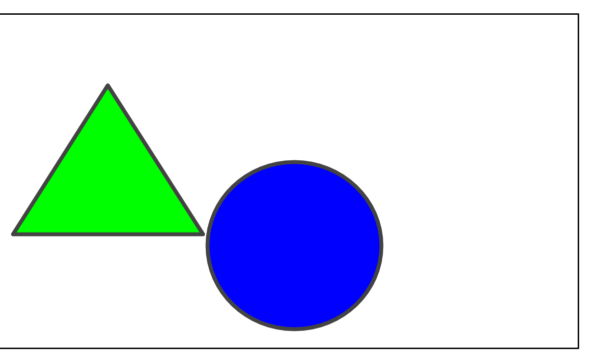
(a) Candidate image

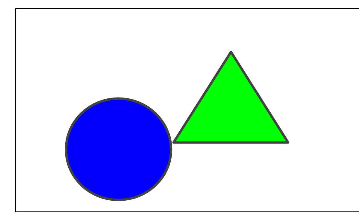
(b) Reference image

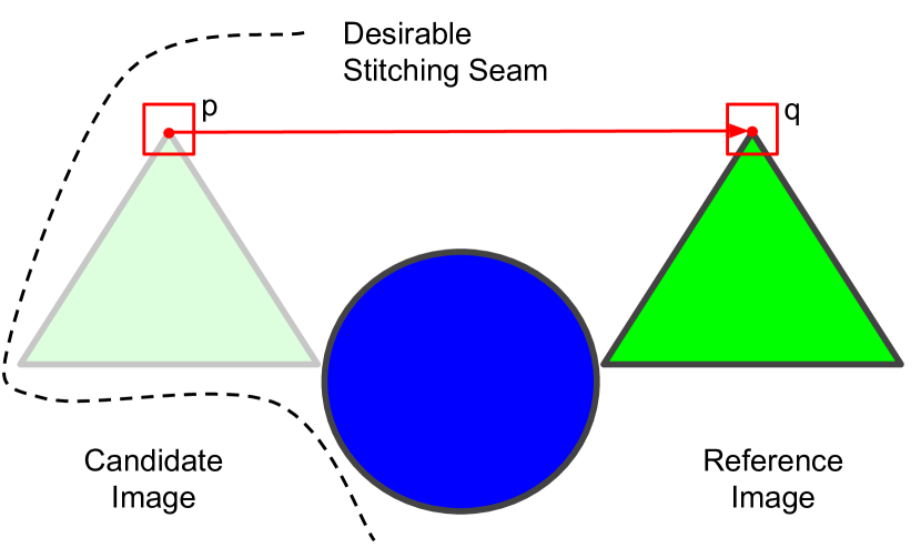
(c) Good stitch

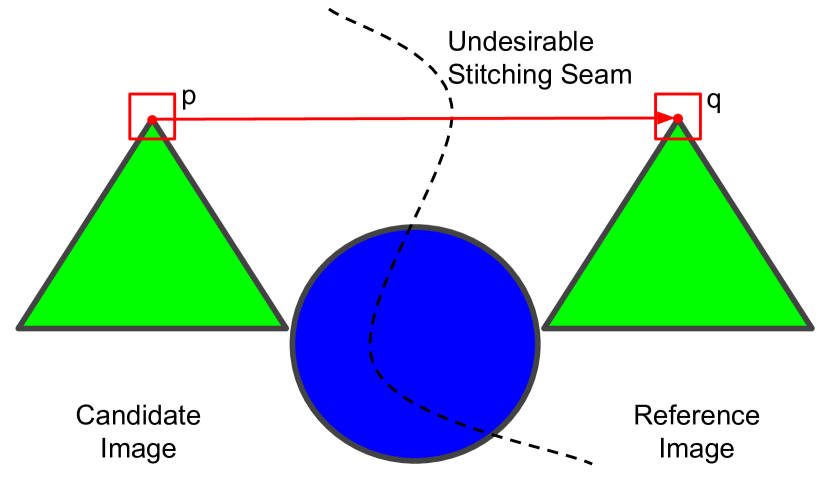
(d) Bad stitch

Figure 4: Illustration of the duplication term. Figure 4(c) provides a bad stitching result with the green triangles duplicated. The feature point correspondence between pixel $p$ and $q$ suggests duplication, and we introduce a term which penalizes this scenario.

Duplication avoidance term. For stitching tasks with large parallax or motion, it is easy to duplicate scene content in the stitching result. We address this issue by explicitly formalizing a duplication avoidance term in our energy. If pixel $p$ from the reference image $I^{S}_{0}$ and $q$ from the candidate image $I^{S}_{i}$ form a true correspondence, then they refer to the same point (i.e., scene element) in the real world. Therefore, we penalize a labeling that contains both of them (i.e., $x_{p}=0,x_{q}=i$), as shown in Figure 4. Since our correspondence is sparse, we also apply this idea to the local region within a radius $r$ of pixels $p$ and $q$. We reweight the penalty by a Gaussian $G$ since the farther away we are from these corresponding pixels, the more uncertain the correspondence.

Formally, our duplication term $E_{c}$ is defined as

$$E_{d}(x)=\lambda_{d}\sum_{i=1}^{N}\sum_{(p,q)\in\mathcal{C}_{i}}\sum_{\delta\in\mathcal{B}_{r}}e_{r}(x_{p+\delta},x_{q+\delta};\delta,i)$$ (2)

where $\mathcal{C}_{i}$ is the pixel correspondence between $I^{S}_{0}$ and $I^{S}_{i}$, and $\mathcal{B}_{r}=\{(dx,dy)\in\mathcal{I}^{2}\mid\|(dx,dy)\|\leq r\}$ is a box of radius $r$. $e_{r}(x_{p+\delta},x_{q+\delta};\delta,i)=G(\|\delta\|)$ when $x_{p}=0,x_{q}=i$, and 0 otherwise.

4 Experimental results and implementation details

Experimental setup. Our goal is to perform stitching on images whose degree of parallax and motion causes previous methods to fail. Ideally, there would be a standard dataset of images that are too difficult to stitch, along with an evaluation metric. Unfortunately this is not the case, in part due to the difficulty of defining ground truth for image stitching. We therefore had to rely on collecting challenging imagery ourselves, though we found one appropriate example (Figure 8) whose stitching failures were widely shared on social media.

We implemented or obtained code for a number of alternative methods, as detailed below, and ran them on all of our examples, along with our technique using a single parameter setting. Since our images are so challenging, it was not uncommon for a competing method to return no output (“failing to stitch”). In the entire corpus of images we examined, we found numerous cases where competing techniques produced dramatic artifacts, while our algorithm had minimal if any errors. We have not found any example images where our technique produces dramatic artifacts and a competitor does not. However, we found a few less challenging images that are well handled by competitors but where we produce small artifacts. These examples, along with other data, images, and additional material omitted here are available online, for reasons of space we focus here on images that provide useful insight. However, the images included here are representative of the performance we have observed on the entire corpus of challenging images we collected.

We follow the experimental setup of [2], who (very much like our work) describe a stitching approach that can handle images with too much parallax for previous techniques. The strongest overall competitor turns out to be Adobe Photoshop 2018’s stitcher Photomerge [11]. While experimental results reported in [2] compare their algorithm with Photoshop 2014, the 2018 version is substantially better, and does an excellent job of stitching images with too many motions for any other competing methods. Therefore, we take Photoshop’s failing on a dataset as a signal that that dataset is particularly challenging; in this section, we show several examples in this section where we successfully stitch such datasets. In addition to Photoshop we downloaded and ran APAP [14], Autostitch [8], and NIS [10]. To produce stitching results from APAP we follow the approach of [2], who extended APAP with seam-finding. Results from all methods are shown in Figure 11 and 11.

Implementation details. For feature extraction and matching, we used DeepMatch [23]. The associated DeepFlow solver was used to generate flows for the optical flow-based warping. We used the Ceres solver [20] for the QP problems that arose when generating multiple registrations, as discussed in section 3.1.

Visual evaluation. Following [2] we review several images from our test set and highlight the strengths and weaknesses of our technique, as well as those of various methods from the literature. All of our results are shown for a single set of parameters.

We observed two classes of stitching errors: warping errors, where the algorithm fails to generate any candidate image that is well-aligned with the reference image; and stitching errors, where the MRF does not produce good output despite the presence of good candidate warps. An example of our technique making a warping error is shown in Figure 9(e), where no warp found by our algorithm continues the parking stall line, causing a visible seam. An example of a stitching error is given in Figure 9(j), where the remainder of the car’s wheel is available in the warp from which our mosaic draws the front wheelwell. Errors may manifest as a number of different kinds of artifacts, such as: tearing (e.g., the arm in Figure 8b); wrong perspective (e.g., the tan background building in Figure 9(b)); or duplication (e.g., the stop sign in 8b), ghosting (e.g., the bollards in Figure 8b), or omission (e.g., the front door of the car in Figure 9(h)) of scene content.

(a) Input images

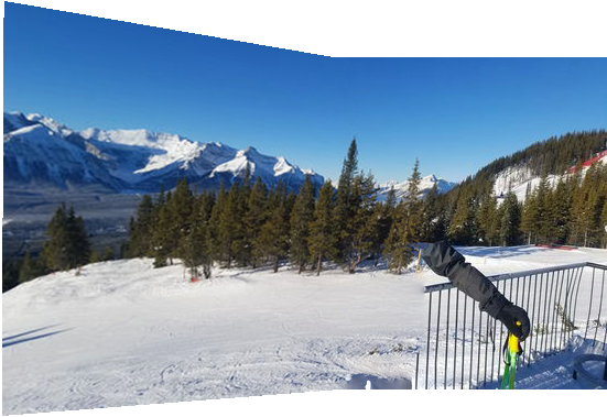
(b) Photoshop [11]

(c) Our result

Figure 5: “Ski” dataset. Photoshop tears the people and the fence. Our stitch has the fence stop abruptly but keeps the people in place. Note that the candidate provides no information that allows us to extend the fence.

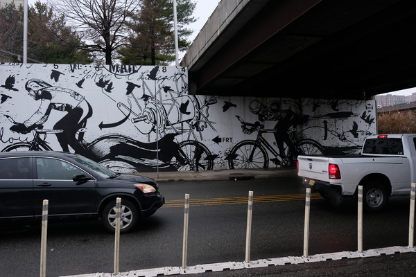
(d) Input images

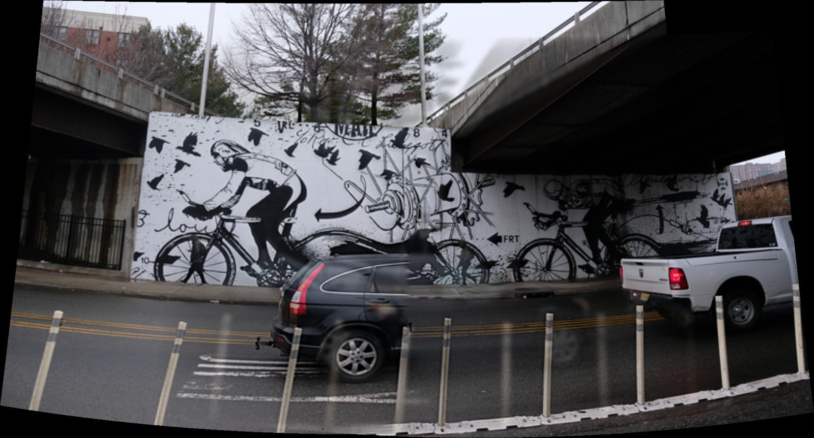
(e) Autostitch [8]

(f) Our result

Figure 6: “Bike Mural” dataset. Autostitch has ghosting on the car, bridge, and poles. Our algorithm shortens the truck and deletes a pole, but has no perceptible ghosting or tearing of the objects.

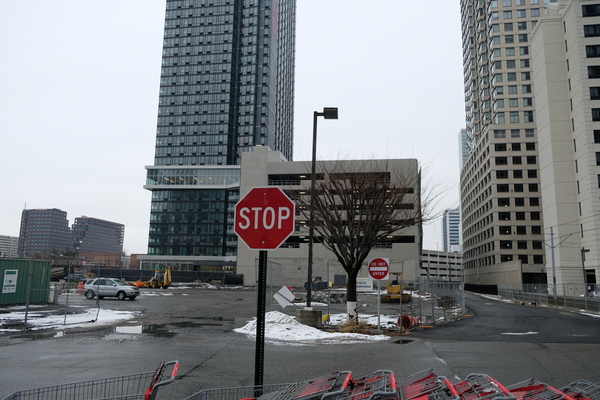
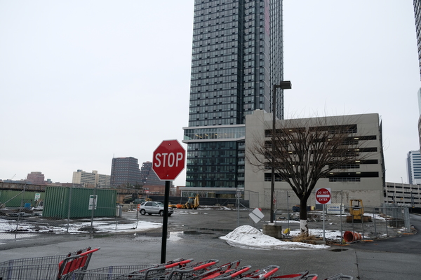
(a) Input images

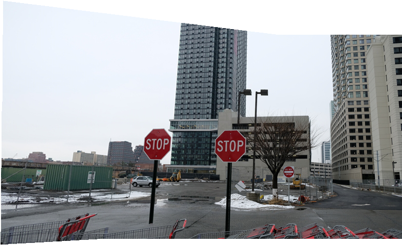
(b) Photoshop [11]

(c) Our result

Figure 7: “Stop Sign” dataset. Photoshop duplicates the stop sign. Of all the implementations we tried, ours is the only visually plausible result, successfully avoiding duplicating the foreground.

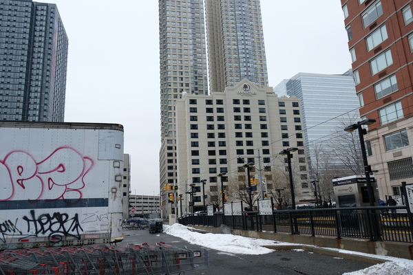
(a) Input images

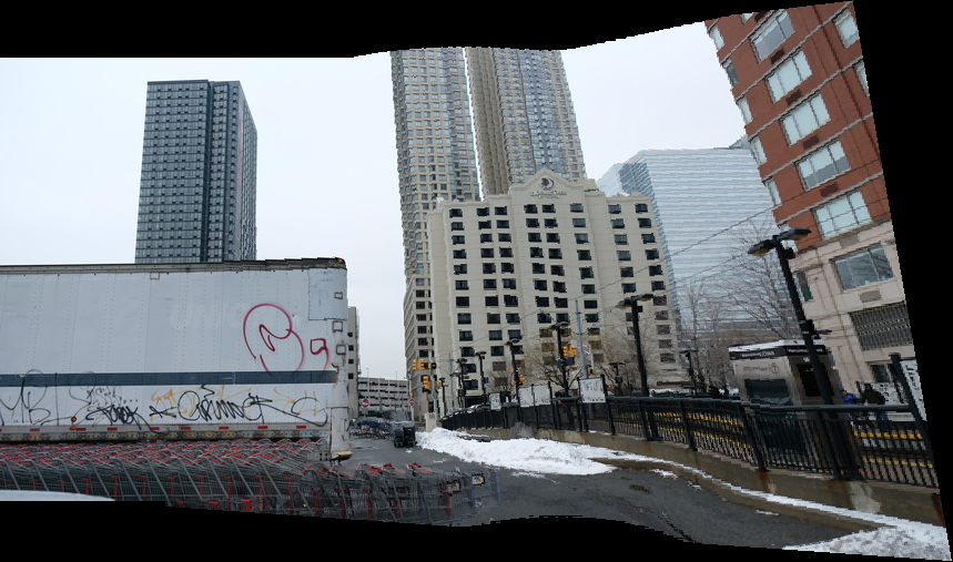
(b) APAP [14]

(c) Our result

Figure 8: “Graffiti-Building” dataset. APAP deletes significant amounts of red graffiti, and introduces noticable curvature. Our result does not produce tearing, ghosting, or duplication.

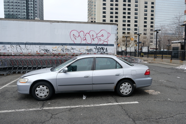
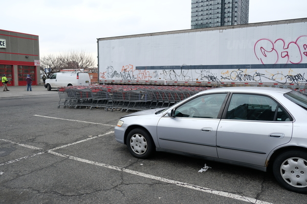
(a) Input images

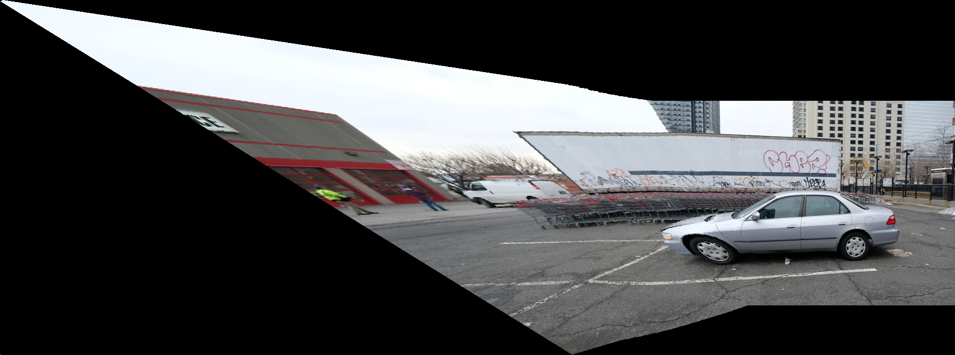
(b) APAP [14]

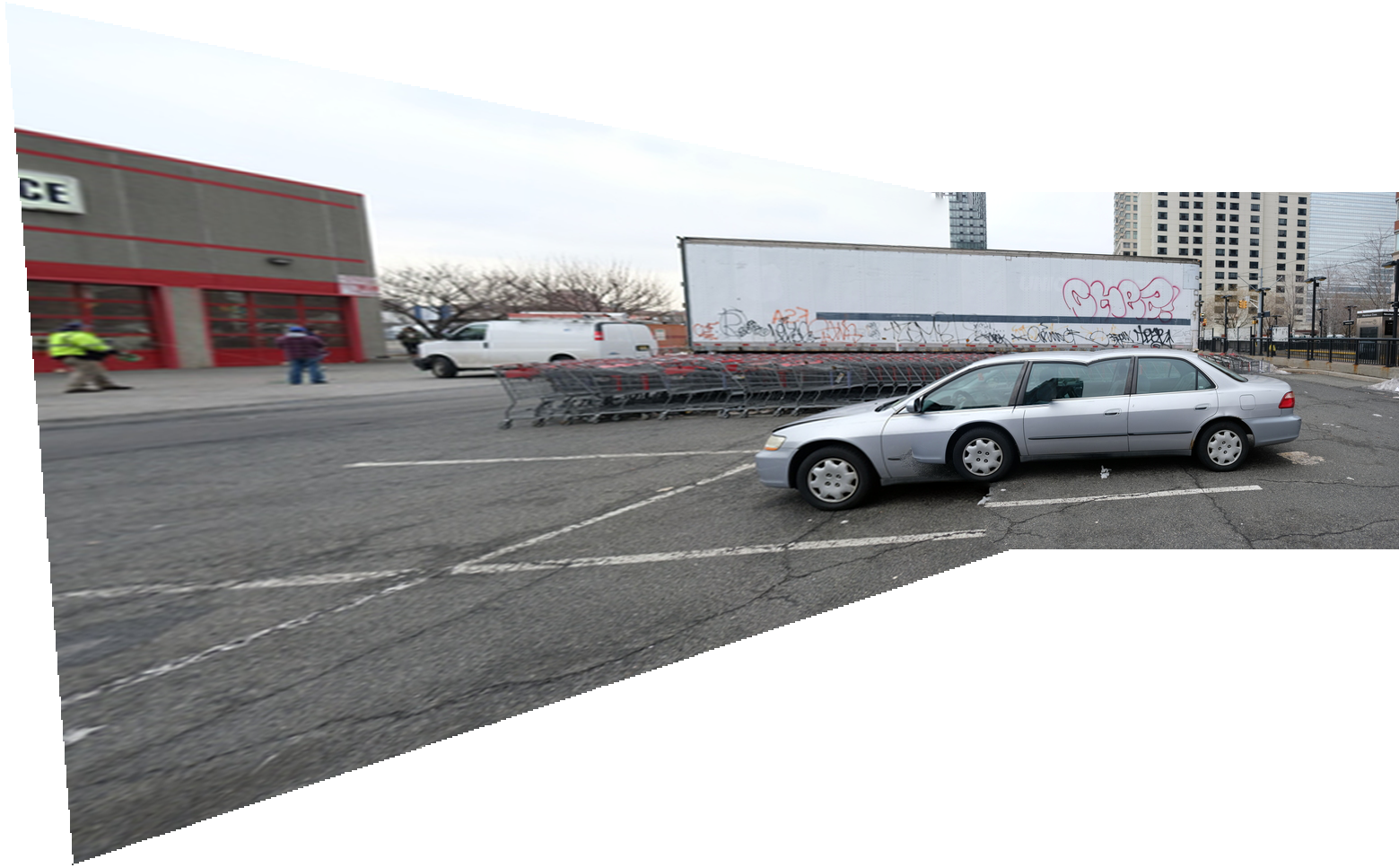
(c) Photoshop [11]

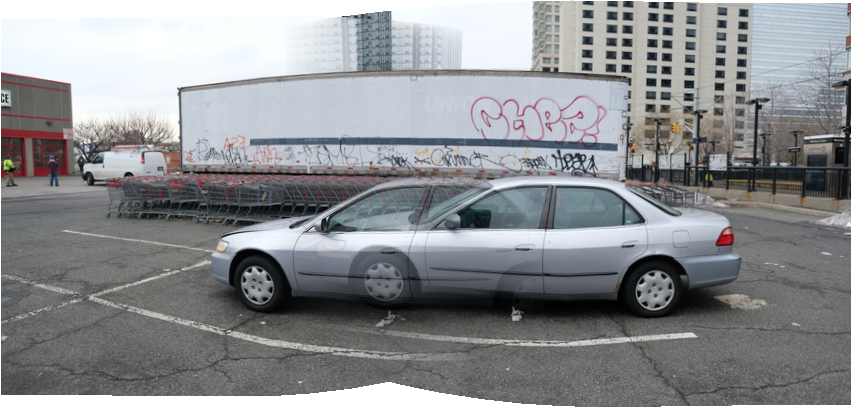
(d) NIS [10]

(e) Our result

Figure 9: “Parking lot” dataset. Autostitch fails to stitch. APAP duplicates the car’s hood , tears a background building, and introduces a corner in the roof of the trailer. Photoshop duplicates the front half of the car. NIS has substantial ghosting. Our result cuts out a part of a parking stall line, but avoids duplicating the car.

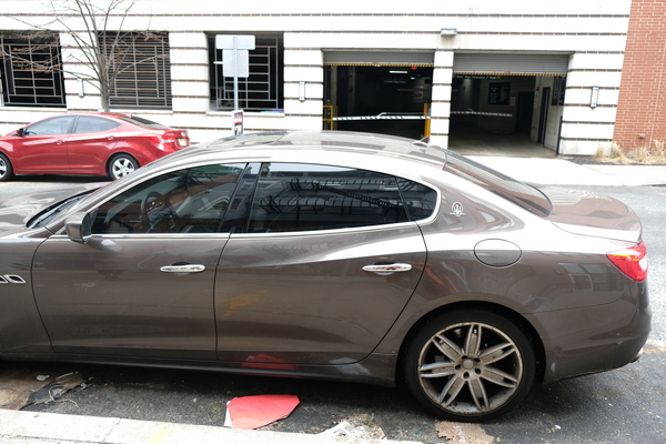
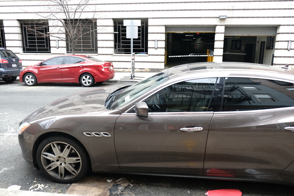
(f) Input images

(g) APAP [14]

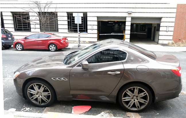
(h) Photoshop [11]

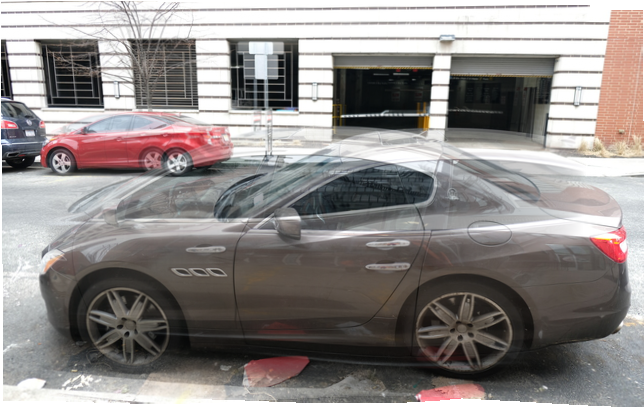
(i) NIS [10]

(j) Our result

Figure 10: “Cars” dataset. Autostitch fails to stitch. APAP and Photoshop shorten the car. APAP also introduces substantial curvature into the background building. NIS has substantial ghosting and shortens the car. Our result deletes part of the hood and front wheel; however, it is the only result which produces an artifact-free car body.

(a) Input images

(b) Our result

Figure 11: An example of tearing and duplication produced by our method.

Quantitative evaluation. The only quantitative metric used by previous stitching papers is seam quality (MRF energy). However, as we have shown, local seam quality is not indicative of stitch quality. Also, this technique requires the user to know the seam location, which precludes it from being run on black-box algorithms like Photoshop. Here we attempt to define a metric to address these problems.

We first observe that stitching can be viewed as a form of view synthesis with weaker assumptions regarding the camera placement or type. With this connection in mind, we redefine perspective stitching as extending the field of view of a reference image using the information in the candidate images. This redefintion naturally leads to an evaluation technique. We crop part of the reference image and then stitch the cropped image with the candidate image. This cropped region serves as a ground truth, which we can compare against the appropriate location in the stitch result. Note that in perspective stitching, the reference image’s size is not altered so we know the exact area where the cropped region should be. We then calculate MS-SSIM [24] or PSNR.

We report this evaluation for 2 examples in Table 1: 50 pixels are cropped off the edge of the reference images in Stop Sign (left side of first image for Figure 8) and Graffiti Building (right side of first image for Figure 8). The stitch results for the cropped images appear almost identical to the stitch results for the whole images. Best score shown inbold. “Ground Truth” compares only the ground truth region to the appropriate location, while “Uncropped Reference” compares the uncropped reference.

Table 1: Evaluation scores for different algorithms.

Image	Comparison	Metric	Ours	APAP [14]	Photoshop [11]
Stop Sign	Ground Truth Region	MS-SSIM	0.6851	0.6573	0.6861
		PSNR	19.4943	17.7073	18.9996
	Uncropped Reference	MS-SSIM	0.9354	0.8981	0.9108
		PSNR	23.0006	20.3533	20.9238
Graffiti Building	Ground Truth Region	MS-SSIM	0.4636	0.3747	0.1250
		PSNR	14.9983	13.1269	9.6520
	Uncropped Reference	MS-SSIM	0.9253	0.5737	0.8541
		PSNR	24.7637	14.8298	18.7102

Note that for Stop Sign, all algorithms performed reasonably in Ground Truth Region. However, both APAP and Photoshop include a duplicate of the stop sign that lowers their values for Uncropped Reference.

5 Conclusions, limitations, and future work

We have demonstrated a novel formulation of the image stitching problem in which multiple candidate registrations are used. We have generalized MRF seam finding to this setting and proposed new terms to combat common artifacts such as object duplication. Our techniques outperform existing algorithms in large parallax and motion scenarios.

Our methods naturally generalize to other stitching surfaces such as cylinders or spheres via modifications to the warping function. Three or more input images can be handled by proposing multiple registrations of each candidate image, and letting the seam finder composite them. A potential problem is the presence of undetected sparse correspondences, which can lead to duplications or tears (Figure 11). The use of dense correspondences may remedy this issue, but our preliminary experiments suggest that optical flows cannot easily capture motion in input images with large disparities, and do not produce correspondences of sufficient quality. A second issue is that it is unclear whether to populate regions of the output mosaic when only data from a single candidate image is present, as the constrained choice of candidate here may conflict with choices made in other regions of the mosaic. This can to some extent be handled with modifications to the data term, but compared to traditional methods, scene content may be lost. One example of this occurs in Figure 11, where the front wheel of the car is omitted in the final output. These problems remain exciting challenges for future work.

5.0.1 Acknowledgements

This research was supported by NSF grants IIS-1161860 and IIS-1447473 and by a Google Faculty Research Award. We thank Connie Choi for help collecting images.

References

- [1] Lin, K., Jiang, N., Cheong, L.F., Do, M., Lu, J.: Seagull: Seam-guided local alignment for parallax-tolerant image stitching. In: ECCV. (2016) 370–385
- [2] Zhang, F., Liu, F.: Parallax-tolerant image stitching. In: CVPR. (2014) 3262–3269
- [3] Willis, J., Argawal, S., Serge, B.: What went where. In: CVPR. (2003) 37–44
- [4] Wang, J., Adelson, E.: Representing moving images with layers. TIP 3(5) (1994) 625–638
- [5] Kwatra, V., Schödl, A., Essa, I., Turk, G., Bobick, A.: Graphcut textures: Image and video synthesis using graph cuts. SIGGRAPH 22(3) (2003) 277–286
- [6] Szeliski, R.: Image alignment and stitching: A tutorial. Foundations and Trends in Computer Graphics and Vision 2(1) (2007) 1–104
- [7] Szeliski, R.: Computer Vision: Algorithms and Applications. Springer (2010)
- [8] Brown, M., Lowe, D.G.: Automatic panoramic image stitching using invariant features. IJCV 74(1) (2007) 59–73
- [9] Perez, P., Gangnet, M., Blake, A.: Poisson image editing. SIGGRAPH (2003) 313–318
- [10] Chen, Y.S., Chuang, Y.Y.: Natural image stitching with the global similarity prior. In: ECCV. (2016) 186–201
- [11] Adobe: Create panoramic images with photomerge. https://helpx.adobe.com/in/photoshop/using/create-panoramic-images-photomerge.html. Accessed: 2018-07-25.
- [12] Adobe: Create and edit panoramic images. https://helpx.adobe.com/photoshop/using/create-panoramic-images-photomerge.html. Accessed: 2018-07-25.
- [13] Shum, H.Y., Szeliski, R.: Construction of panoramic image mosaics with global and local alignment. In: Panoramic vision. (2001) 227–268
- [14] Zaragoza, J., Chin, T.J., Brown, M.S., Suter, D.: As-projective-as-possible image stitching with moving dlt. In: CVPR. (2013) 2339–2346
- [15] Lin, C.C., Pankanti, S.U., Natesan Ramamurthy, K., Aravkin, A.Y.: Adaptive as-natural-as-possible image stitching. In: CVPR. (2015) 1155–1163
- [16] Szeliski, R., Zabih, R., Scharstein, D., Veksler, O., Kolmogorov, V., Agarwala, A., Tappen, M., Rother, C.: A comparative study of energy minimization methods for Markov Random Fields. TPAMI 30(6) (2008) 1068–1080
- [17] Agarwala, A., Dontcheva, M., Agrawala, M., Drucker, S., Colburn, A., Curless, B., Salesin, D., Cohen, M.: Interactive digital photomontage. SIGGRAPH 23(3) (2004) 294–302
- [18] Burt, P., Adelson, E.: A multiresolution spline with application to image mosaics. SIGGRAPH 2(4) (1983) 217–236
- [19] Bradski, G.: The OpenCV Library. Dr. Dobb’s Journal of Software Tools (2000)
- [20] Agarwal, S., Mierle, K., Others: Ceres solver. http://ceres-solver.org. Accessed: 2018-07-25.
- [21] Liu, F., Gleicher, M., Jin, H., Agarwala, A.: Content-preserving warps for 3D video stabilization. SIGGRAPH 28(3) (2009)
- [22] Boykov, Y., Veksler, O., Zabih, R.: Fast approximate energy minimization via graph cuts. TPAMI 23(11) (2001) 1222–1239
- [23] Weinzaepfel, P., Revaud, J., Harchaoui, Z., Schmid, C.: Deepflow: Large displacement optical flow with deep matching. In: ICCV. (2013) 1385–1392
- [24] Wang, Z., Simoncelli, E., Bovik, A.: Multiscale structural similarity for image quality assessment. In: Asilomar Conference on Signals, Systems and Computers. (2004) 1398–1402