The Reads-From Equivalence for the TSO and PSO Memory Models

Abstract.

The verification of concurrent programs remains an open challenge due to the non-determinism in inter-process communication. One recurring algorithmic problem in this challenge is the consistency verification of concurrent executions. In particular, consistency verification under a reads-from map allows to compute the reads-from (RF) equivalence between concurrent traces, with direct applications to areas such as Stateless Model Checking (SMC). Importantly, the RF equivalence was recently shown to be coarser than the standard Mazurkiewicz equivalence, leading to impressive scalability improvements for SMC under $\operatorname{SC}$ (sequential consistency). However, for the relaxed memory models of $\operatorname{TSO}$ and $\operatorname{PSO}$ (total/partial store order), the algorithmic problem of deciding the RF equivalence, as well as its impact on SMC, has been elusive.

In this work we solve the algorithmic problem of consistency verification for the $\operatorname{TSO}$ and $\operatorname{PSO}$ memory models given a reads-from map, denoted $\operatorname{VTSO-rf}$ and $\operatorname{VPSO-rf}$, respectively. For an execution of $n$ events over $k$ threads and $d$ variables, we establish novel bounds that scale as $n^{k+1}$ for $\operatorname{TSO}$ and as $n^{k+1}\cdot\min(n^{k^{2}},2^{k\cdot d})$ for $\operatorname{PSO}$. Moreover, based on our solution to these problems, we develop an SMC algorithm under $\operatorname{TSO}$ and $\operatorname{PSO}$ that uses the RF equivalence. The algorithm is exploration-optimal, in the sense that it is guaranteed to explore each class of the RF partitioning exactly once, and spends polynomial time per class when $k$ is bounded. Finally, we implement all our algorithms in the SMC tool Nidhugg, and perform a large number of experiments over benchmarks from existing literature. Our experimental results show that our algorithms for $\operatorname{VTSO-rf}$ and $\operatorname{VPSO-rf}$ provide significant scalability improvements over standard alternatives. Moreover, when used for SMC, the RF partitioning is often much coarser than the standard Shasha–Snir partitioning for $\operatorname{TSO}/\operatorname{PSO}$, which yields a significant speedup in the model checking task.

1. INTRODUCTION

The formal analysis of concurrent programs is a key problem in program analysis and verification. Scheduling non-determinism makes programs both hard to write correctly, and to analyze formally, as both the programmer and the model checker need to account for all possible communication patterns among threads. This non-determinism incurs an exponential blow-up in the state space of the program, which in turn yields a significant computational cost on the verification task.

Traditional verification has focused on concurrent programs adhering to sequential consistency (Lamport, 1979). Programs operating under relaxed memory semantics exhibit additional behavior compared to sequential consistency. This makes it exceptionally hard to reason about correctness, as, besides scheduling subtleties, the formal reasoning needs to account for buffer/caching mechanisms. Two of the most standard operational relaxed memory models in the literature are Total Store Order ($\operatorname{TSO}$) and Partial Store Order ($\operatorname{PSO}$) (Adve and Gharachorloo, 1996; SPARC International, 1994; Owens et al., 2009; Sewell et al., 2010; Alglave et al., 2017; Alglave, 2010).

On the operational level, both models introduce subtle mechanisms via which write operations become visible to the shared memory and thus to the whole system. Under $\operatorname{TSO}$, every thread is equipped with its own buffer. Every write to a shared variable is pushed into the buffer, and thus remains hidden from the other threads. The buffer is flushed non-deterministically to the shared memory, at which point the writes become visible to the other threads. The semantics under $\operatorname{PSO}$ are even more involved, as now every thread has one buffer per shared variable, and non-determinism now governs not only when a thread flushes its buffers, but also which buffers are flushed.

Th $$\text{read}_{1}$$

$$1.\leavevmode\nobreak\ {\color[rgb]{0,0,0.8}w(x)}$$

$$2.\leavevmode\nobreak\ {\color[rgb]{0.8,0,0}\operatorname{r}(y)}$$

Th $$\text{read}_{2}$$

$$1.\leavevmode\nobreak\ {\color[rgb]{0.8,0,0}w^{\prime}(y)}$$

$$2.\leavevmode\nobreak\ {\color[rgb]{0,0,0.8}\operatorname{r}^{\prime}(x)}$$

Th $$\text{read}_{1}$$

$$1.\leavevmode\nobreak\ {\color[rgb]{0,0,0.8}w(x)}$$

$$2.\leavevmode\nobreak\ {\color[rgb]{0.8,0,0}w^{\prime}(y)}$$

Th $$\text{read}_{2}$$

$$1.\leavevmode\nobreak\ {\color[rgb]{0.8,0,0}\operatorname{r}(y)}$$

$$2.\leavevmode\nobreak\ {\color[rgb]{0,0,0.8}\operatorname{r}^{\prime}(x)}$$

Figure 1. A TSO example (left) and a PSO example (right).

To illustrate the intricacies under $\operatorname{TSO}$ and $\operatorname{PSO}$, consider the examples in Figure 1. On the left, under $\operatorname{SC}$, in every execution at least one of $\operatorname{r}(y)$ and $\operatorname{r}^{\prime}(x)$ will observe the corresponding $w^{\prime}(y)$ and $w(x)$. Under $\operatorname{TSO}$, however, the write events may become visible on the shared memory only after the read events have executed, and hence both write events go unobserved. Executions under $\operatorname{PSO}$ are even more involved, see Figure 1 right. Under either $\operatorname{SC}$ or $\operatorname{TSO}$, if $\operatorname{r}(y)$ observes $w^{\prime}(y)$, then $\operatorname{r}^{\prime}(x)$ must observe $w(x)$, as $w(x)$ becomes visible on the shared memory before $w^{\prime}(y)$. Under $\operatorname{PSO}$, however, there is a single local buffer for each variable. Hence the order in which $w(x)$ and $w^{\prime}(y)$ become visible in the shared memory can be reversed, allowing $\operatorname{r}(y)$ to observe $w^{\prime}(y)$ while $\operatorname{r}^{\prime}(x)$ does not observe $w(x)$.

The great challenge in verification under relaxed memory is to systematically, yet efficiently, explore all such extra behaviors of the system, i.e., account for the additional non-determinism that comes from the buffers. In this work we tackle this challenge for two verification tasks under $\operatorname{TSO}$ and $\operatorname{PSO}$, namely, (A) for verifying the consistency of executions, and (B) for stateless model checking.

A. Verifying execution consistency with a reads-from function.

One of the most basic problems for a given memory model is the verification of the consistency of program executions with respect to the given model (Chini and Saivasan, 2020). The input is a set of thread executions, where each execution performs operations accessing the shared memory. The task is to verify whether the thread executions can be interleaved to a concurrent execution, which has the property that every read observes a specific value written by some write (Gibbons and Korach, 1997). The problem is of foundational importance to concurrency, and has been studied heavily under $\operatorname{SC}$ (Chen et al., 2009; Cain and Lipasti, 2002; Hu et al., 2012).

The input is often enhanced with a reads-from (RF) map, which further specifies for each read access the write access that the former should observe. Under sequential consistency, the corresponding problem $\operatorname{VSC-rf}$ was shown to be $NP$-hard in the landmark work of Gibbons and Korach (1997), while it was recently shown $\operatorname{W[1]}$-hard (Mathur et al., 2020). The problem lies at the heart of many verification tasks in concurrency, such as dynamic analyses (Smaragdakis et al., 2012; Kini et al., 2017; Pavlogiannis, 2019; Mathur et al., 2020; Roemer et al., 2020; Mathur et al., 2021), linearizability and transactional consistency (Herlihy and Wing, 1990; Biswas and Enea, 2019), as well as SMC (Abdulla et al., 2019; Chalupa et al., 2017; Kokologiannakis et al., 2019b).

Executions under relaxed memory.

The natural extension of verifying execution consistency with an RF map is from $\operatorname{SC}$ to relaxed memory models such as $\operatorname{TSO}$ and $\operatorname{PSO}$, we denote the respective problems by $\operatorname{VTSO-rf}$ and $\operatorname{VPSO-rf}$. Given the importance of $\operatorname{VSC-rf}$ for $\operatorname{SC}$, and the success in establishing both upper and lower bounds, the complexity of $\operatorname{VTSO-rf}$ and $\operatorname{VPSO-rf}$ is a very natural question and of equal importance. The verification problem is known to be $NP$-hard for most memory models (Furbach et al., 2015), including $\operatorname{TSO}$ and $\operatorname{PSO}$, however, no other bounds are known. Some heuristics have been developed for $\operatorname{VTSO-rf}$ (Manovit and Hangal, 2006; Zennou et al., 2019), while other works study $\operatorname{TSO}$ executions that are also sequentially consistent (Bouajjani et al., 2011, 2013).

B. Stateless Model Checking.

The most standard solution to the space-explosion problem is stateless model checking (Godefroid, 1996). Stateless model-checking methods typically explore traces rather than states of the analyzed program. The depth-first nature of the exploration enables it to be both systematic and memory-efficient, by storing only a few traces at any given time. Stateless model-checking techniques have been employed successfully in several well-established tools, e.g., VeriSoft (Godefroid, 1997, 2005) and CHESS (Madan Musuvathi, 2007).

As there are exponentially many interleavings, a trace-based exploration typically has to explore exponentially many traces, which is intractable in practice. One standard approach is the partitioning of the trace space into equivalence classes, and then attempting to explore every class via a single representative trace. The most successful adoption of this technique is in dynamic partial order reduction (DPOR) techniques (Clarke et al., 1999; Godefroid, 1996; Peled, 1993; Flanagan and Godefroid, 2005). The great advantage of DPOR is that it handles indirect memory accesses precisely without introducing spurious interleavings. The foundation underpinning DPOR is the famous Mazurkiewicz equivalence, which constructs equivalence classes based on the order in which traces execute conflicting memory access events. This idea has led to a rich body of work, with improvements using symbolic techniques (Kahlon et al., 2009), context-sensitivity (Albert et al., 2017), unfoldings (Rodríguez et al., 2015), effective lock handling (Kokologiannakis et al., 2019a), and others (Aronis et al., 2018; Albert et al., 2018; Chatterjee et al., 2019). The work of Abdulla et al. (2014) developed an SMC algorithm that is exploration-optimal for the Mazurkiewicz equivalence, in the sense that it explores each class of the underlying partitioning exactly once. Finally, techniques based on SAT/SMT solvers have been used to construct even coarser partitionings (Demsky and Lam, 2015; Huang, 2015; Huang and Huang, 2017).

The reads-from equivalence for SMC.

A new direction of SMC techniques has been recently developed using the reads-from (RF) equivalence to partition the trace space. The key principle is to classify traces as equivalent based on whether read accesses observe the same write accesses. The idea was initially explored for acyclic communication topologies (Chalupa et al., 2017), and has been recently extended to all topologies (Abdulla et al., 2019). As the RF partitioning is guaranteed to be (even exponentially) coarser than the Mazurkiewicz partitioning, SMC based on RF has shown remarkable scalability potential (Abdulla et al., 2019; Abdulla et al., 2018; Kokologiannakis et al., 2019b; Kokologiannakis and Vafeiadis, 2020). The key technical component for SMC using RF is the verification of execution consistency, as presented in the previous section. The success of SMC using RF under $\operatorname{SC}$ has thus rested upon new efficient methods for the problem $\operatorname{VSC-rf}$.

SMC under relaxed memory.

The SMC literature has taken up the challenge of model checking concurrent programs under relaxed memory. Extensions to SMC for $\operatorname{TSO}/\operatorname{PSO}$ have been considered by Zhang et al. (2015) using shadow threads to model memory buffers, as well as by Abdulla et al. (2015) using chronological traces to represent the Shasha–Snir notion of trace under relaxed memory (Shasha and Snir, 1988). Chronological/Shasha–Snir traces are the generalization of Mazurkiewicz traces to $\operatorname{TSO}/\operatorname{PSO}$. Further extensions have also been made to other memory models, namely by Abdulla et al. (2018) for the release-acquire fragment of C++11, Kokologiannakis et al. (2017, 2019b) for the RC11 model (Lahav et al., 2017), and Kokologiannakis and Vafeiadis (2020) for the IMM model (Podkopaev et al., 2019), but notably none for $\operatorname{TSO}$ and $\operatorname{PSO}$ using the RF equivalence. Given the advantages of the RF equivalence for SMC under $\operatorname{SC}$ (Abdulla et al., 2019), release-acquire (Abdulla et al., 2018), RC11 (Kokologiannakis et al., 2019b) and IMM (Kokologiannakis and Vafeiadis, 2020), a very natural standing question is whether RF can be used for effective SMC under $\operatorname{TSO}$ and $\operatorname{PSO}$. Here we tackle this challenge.

1.1. Our Contributions

Here we outline the main results of our work. We refer to Section 3 for a formal presentation.

A. Verifying execution consistency for $\operatorname{TSO}$ and $\operatorname{PSO}$.

Our first set of results and the main contribution of this paper is on the problems $\operatorname{VTSO-rf}$ and $\operatorname{VPSO-rf}$ for verifying $\operatorname{TSO}$- and $\operatorname{PSO}$-consistent executions, respectively. Consider an input to the corresponding problem that consists of $k$ threads and $n$ operations, where each thread executes write and read operations, as well as fence operations that flush each thread-local buffer to the main memory. Our results are as follows.

1. We present an algorithm that solves $\operatorname{VTSO-rf}$ in $O(k\cdot n^{k+1})$ time. The case of $\operatorname{VSC-rf}$ is solvable in $O(k\cdot n^{k})$ time (Abdulla et al., 2019; Biswas and Enea, 2019; Mathur et al., 2020). Although for $\operatorname{TSO}$ there are $k$ additional buffers, our result shows that the complexity is only minorly impacted by an additional factor $n$, as opposed to $n^{k}$.

2. We present an algorithm that solves $\operatorname{VPSO-rf}$ in $O(k\cdot n^{k+1}\cdot\min(n^{k\cdot(k-1)},2^{k\cdot d}))$ time, where $d$ is the number of variables. Note that even though there are $k\cdot d$ buffers, one of our two bounds is independent of $d$ and thus yields polynomial time when the number of threads is bounded. Moreover, our bound collapses to $O(k\cdot n^{k+1})$ when there are no fences, and hence this case is no more difficult that $\operatorname{VTSO-rf}$.

B. Stateless model checking for $\operatorname{TSO}$ and $\operatorname{PSO}$ using the reads-from equivalence (RF).

Our second contribution is an algorithm $\operatorname{RF-SMC}$ for SMC under $\operatorname{TSO}$ and $\operatorname{PSO}$ using the RF equivalence. The algorithm is based on the reads-from algorithm for $\operatorname{SC}$ (Abdulla et al., 2019) and uses our solutions to $\operatorname{VTSO-rf}$ and $\operatorname{VPSO-rf}$ for visiting each class of the respective partitioning. Moreover, $\operatorname{RF-SMC}$ is exploration-optimal, in the sense that it explores only maximal traces and further it is guaranteed to explore each class of the RF partitioning exactly once. For the complexity statements, let $k$ be the total number of threads and $n$ be the number of events of the longest trace. The time spent by $\operatorname{RF-SMC}$ per class of the RF partitioning is

1. $n^{O(k)}$ time, for the case of $\operatorname{TSO}$, and

2. $n^{O(k^{2})}$ time, for the case of $\operatorname{PSO}$.

Note that the time complexity per class is polynomial in $n$ when $k$ is bounded.

C. Implementation and experiments.

We have implemented $\operatorname{RF-SMC}$ in the stateless model checker Nidhugg (Abdulla et al., 2015), and performed an evaluation on an extensive set of benchmarks from the recent literature. Our results show that our algorithms for $\operatorname{VTSO-rf}$ and $\operatorname{VPSO-rf}$ provide significant scalability improvements over standard alternatives, often by orders of magnitude. Moreover, when used for SMC, the RF partitioning is often much coarser than the standard Shasha–Snir partitioning for $\operatorname{TSO}/\operatorname{PSO}$, which yields a significant speedup in the model checking task.

2. PRELIMINARIES

General notation. Given a natural number $i\geq 1$, we let $[i]$ be the set $\{1,2,\dots,i\}$. Given a map $f\colon X\to Y$, we let $\mathsf{dom}(f)=X$ and $\mathsf{img}(f)=Y$ denote the domain and image of $f$, respectively. We represent maps $f$ as sets of tuples $\{(x,f(x))\}_{x}$. Given two maps $f_{1},f_{2}$ over the same domain $X$, we write $f_{1}=f_{2}$ if for every $x\in X$ we have $f_{1}(x)=f_{2}(x)$. Given a set $X^{\prime}\subset X$, we denote by $f|X^{\prime}$ the restriction of $f$ to $X^{\prime}$. A binary relation $\sim$ on a set $X$ is an equivalence iff $\sim$ is reflexive, symmetric and transitive. We denote by $X/\sim$ the quotient (i.e., the set of all equivalence classes) of $X$ under $\sim$.

2.1. Concurrent Model under $\operatorname{TSO}$/$\operatorname{PSO}$

Here we describe the computational model of concurrent programs with shared memory under the Total Store Order ($\operatorname{TSO}$) and Partial Store Order ($\operatorname{PSO}$) memory models. We follow a standard exposition, similarly to Abdulla et al. (2015); Huang and Huang (2016). We first describe $\operatorname{TSO}$ and then extend our description to $\operatorname{PSO}$.

Concurrent program with Total Store Order.

We consider a concurrent program $\mathscr{P}=\{\mathsf{thr}_{i}\}_{i=1}^{k}$ of $k$ threads. The threads communicate over a shared memory $\mathcal{G}$ of global variables. Each thread additionally owns a store buffer, which is a FIFO queue for storing updates of variables to the shared memory. Threads execute events of the following types.

1. A buffer-write event $\operatorname{wB}$ enqueues into the local store buffer an update that wants to write a value $v$ to a global variable $x\in\mathcal{G}$.

2. A read event $\operatorname{r}$ reads the value $v$ of a global variable $x\in\mathcal{G}$. The value $v$ is the value of the most recent local buffer-write event, if one still exists in the buffer, otherwise $v$ is the value of $x$ in the shared memory.

Additionally, whenever a store buffer of some thread is nonempty, the respective thread can execute the following.

1. A memory-write event $\operatorname{wM}$ that dequeues the oldest update from the local buffer and performs the corresponding write-update on the shared memory.

Threads can also flush their local buffers into the memory using fences.

1. A fence event $\operatorname{fnc}$ blocks the corresponding thread until its store buffer is empty.

Finally, threads can execute local events that are not modeled explicitly, as usual. We refer to all non-memory-write events as thread events. Following the typical setting of stateless model checking (Flanagan and Godefroid, 2005; Abdulla et al., 2014; Abdulla et al., 2015; Chalupa et al., 2017), each thread of the program $\mathscr{P}$ is deterministic, and further $\mathscr{P}$ is bounded, meaning that all executions of $\mathscr{P}$ are finite and the number of events of $\mathscr{P}$’s longest execution is a parameter of the input.

Given an event $e$, we denote by $\mathsf{thr}(e)$ its thread and by $\mathsf{var}(e)$ its global variable. We denote by $\mathcal{E}$ the set of all events, by $\mathcal{R}$ the set of read events, by $\mathcal{W}^{B}$ the set of buffer-write events, by $\mathcal{W}^{M}$ the set of memory-write events, and by $\mathcal{F}$ the set of fence events. Given a buffer-write event $\operatorname{wB}\in\mathcal{W}^{B}$ and its corresponding memory-write $\operatorname{wM}\in\mathcal{W}^{M}$, we let $\mathbf{w}=(\operatorname{wB},\operatorname{wM})$ be the two-phase write event, and we denote $\mathsf{thr}(\mathbf{w})=\mathsf{thr}(\operatorname{wB})=\mathsf{thr}(\operatorname{wM})$ and $\mathsf{var}(\mathbf{w})=\mathsf{var}(\operatorname{wB})=\mathsf{var}(\operatorname{wM})$. We denote by $\mathcal{W}$ the set of all such two-phase write events. Given two events $e_{1},e_{2}\in\mathcal{R}\cup\mathcal{W}^{M}$, we say that they conflict, denoted $e_{1}\Join e_{2}$, if they access the same global variable and at least one of them is a memory-write event.

Proper event sets.

Given a set of events $X\subseteq\mathcal{E}$, we write $\mathcal{R}(X)=X\cap\mathcal{R}$ for the set of read events of $X$, and similarly $\mathcal{W}^{B}(X)=X\cap\mathcal{W}^{B}$ and $\mathcal{W}^{M}(X)=X\cap\mathcal{W}^{M}$ for the buffer-write and memory-write events of $X$, respectively. We also denote by $\mathcal{L}(X)=X\setminus\mathcal{W}^{M}(X)$ the thread events (i.e., the non-memory-write events) of $X$. We write $\mathcal{W}(X)=(X\times X)\cap\mathcal{W}$ for the set of two-phase write events in $X$. We call $X$ proper if $\operatorname{wB}\in X$ iff $\operatorname{wM}\in X$ for each $(\operatorname{wB},\operatorname{wM})\in\mathcal{W}$. Finally, given a set of events $X\subseteq\mathcal{E}$ and a thread $\mathsf{thr}$, we denote by $X_{\mathsf{thr}}$ and $X_{\neq\mathsf{thr}}$ the events of $\mathsf{thr}$, and the events of all other threads in $X$, respectively.

Sequences and Traces.

Given a sequence of events $\tau=e_{1},\dots,e_{j}$, we denote by $\mathcal{E}(\tau)$ the set of events that appear in $\tau$. We further denote $\mathcal{R}(\tau)=\mathcal{R}(\mathcal{E}(\tau))$, $\mathcal{W}^{B}(\tau)=\mathcal{W}^{B}(\mathcal{E}(\tau))$, $\mathcal{W}^{M}(\tau)=\mathcal{W}^{M}(\mathcal{E}(\tau))$, and $\mathcal{W}(\tau)=\mathcal{W}(\mathcal{E}(\tau))$. Finally we denote by $\epsilon$ an empty sequence.

Given a sequence $\tau$ and two events $e_{1},e_{2}\in\mathcal{E}(\tau)$, we write $e_{1}<_{\tau}e_{2}$ when $e_{1}$ appears before $e_{2}$ in $\tau$, and $e_{1}\leq_{\tau}e_{2}$ to denote that $e_{1}<_{\tau}e_{2}$ or $e_{1}=e_{2}$. Given a sequence $\tau$ and a set of events $A$, we denote by $\tau|A$ the projection of $\tau$ on $A$, which is the unique sub-sequence of $\tau$ that contains all events of $A\cap\mathcal{E}(\tau)$, and only those. Given a sequence $\tau$ and an event $e\in\mathcal{E}(\tau)$, we denote by $\mathsf{pre}_{\tau}(e)$ the prefix up until and including $e$, formally $\tau|\{e^{\prime}\in\mathcal{E}(\tau)\,|\,e^{\prime}\leq_{\tau}e\}$. Given two sequences $\tau_{1}$ and $\tau_{2}$, we denote by $\tau_{1}\circ\tau_{2}$ the sequence that results in appending $\tau_{2}$ after $\tau_{1}$.

A (concrete, concurrent) trace is a sequence of events $\sigma$ that corresponds to a concrete valid execution of $\mathscr{P}$ under standard semantics (Shasha and Snir, 1988). We let $\mathsf{enabled}(\sigma)$ be the set of enabled events after $\sigma$ is executed, and call $\sigma$ maximal if $\mathsf{enabled}(\sigma)=\emptyset$. A concrete local trace $\rho$ is a sequence of thread events of the same thread.

Reads-from functions.

Given a proper event set $X\subseteq\mathcal{E}$, a reads-from function over $X$ is a function that maps each read event of $X$ to some two-phase write event of $X$ accessing the same global variable. Formally, $\mathsf{RF}\colon\mathcal{R}(X)\to\mathcal{W}(X)$, where $\mathsf{var}(\operatorname{r})=\mathsf{var}(\mathsf{RF}(\operatorname{r}))$ for all $\operatorname{r}\in\mathcal{R}(X)$. Given a buffer-write event $\operatorname{wB}$ (resp. a memory-write event $\operatorname{wM}$), we write $\mathsf{RF}(\operatorname{r})=(\operatorname{wB},\_)$ (resp. $\mathsf{RF}(\operatorname{r})=(\_,\operatorname{wM})$) to denote that $\mathsf{RF}(\operatorname{r})$ is a two-phase write for which $\operatorname{wB}$ (resp. $\operatorname{wM}$) is the corresponding buffer-write (resp. memory-write) event.

Given a sequence of events $\tau$ where the set $\mathcal{E}(\tau)$ is proper, we define the reads-from function of $\tau$, denoted $\mathsf{RF}_{\tau}\colon\mathcal{R}(\tau)\to\mathcal{W}(\tau)$, as follows. Given a read event $\operatorname{r}\in\mathcal{R}(\tau)$, consider the set $\mathsf{Upd}$ of enqueued conflicting updates in the same thread that have not yet been dequeued, i.e., $\mathsf{Upd}=\{(\operatorname{wB},\operatorname{wM})\in(\mathcal{W}(\tau))_{\mathsf{thr}(\operatorname{r})}\ |\ \operatorname{wM}\Join\operatorname{r},\;\operatorname{wB}<_{\tau}\operatorname{r}<_{\tau}\operatorname{wM}\}$. Then, $\mathsf{RF}_{\tau}(\operatorname{r})=(\operatorname{wB}^{\prime},\operatorname{wM}^{\prime})$, where one of the two cases happens:

• $\mathsf{Upd}\neq\emptyset$, and $(\operatorname{wB}^{\prime},\operatorname{wM}^{\prime})\in\mathsf{Upd}$ is the latest in $\tau$, i.e., for each $(\operatorname{wB}^{\prime\prime},\operatorname{wM}^{\prime\prime})\in\mathsf{Upd}$ we have $\operatorname{wB}^{\prime\prime}\leq_{\tau}\operatorname{wB}^{\prime}$.

• $\mathsf{Upd}=\emptyset$, and $\operatorname{wM}^{\prime}\in\mathcal{W}^{M}(\tau),\,\operatorname{wM}^{\prime}\Join\operatorname{r},\,\operatorname{wM}^{\prime}<_{\tau}\operatorname{r}$ is the latest memory-write (of any thread) conflicting with $\operatorname{r}$ and occurring before $\operatorname{r}$ in $\tau$, i.e., for each $\operatorname{wM}^{\prime\prime}\in\mathcal{W}^{M}(\tau)$ such that $\operatorname{wM}^{\prime\prime}\Join\operatorname{r}$ and $\operatorname{wM}^{\prime\prime}<_{\tau}\operatorname{r}$, we have $\operatorname{wM}^{\prime\prime}\leq_{\tau}\operatorname{wM}^{\prime}$.

Notice how relaxed memory comes into play in the above definition, as $\mathsf{RF}_{\tau}(\operatorname{r})$ does not record which of the two above cases actually happened.

Partial Store Order and Sequential Consistency.

The memory model of Partial Store Order ($\operatorname{PSO}$) is more relaxed than $\operatorname{TSO}$. On the operational level, each thread is equipped with a store buffer for each global variable, rather than a single buffer for all global variables. Then, at any point during execution, a thread can non-deterministically dequeue and perform the oldest update from any of its nonempty store buffers. The notions of events, traces and reads-from functions remain the same for $\operatorname{PSO}$ as defined for $\operatorname{TSO}$. The Sequential Consistency ($\operatorname{SC}$) memory model can be simply thought of as a model where each thread flushes its buffer immediately after a write event, e.g., by using a fence.

Concurrent program semantics.

The semantics of $\mathscr{P}$ are defined by means of a transition system over a state space of global states. A global state consists of (i) a memory function that maps every global variable to a value, (ii) a local state for each thread, which contains the values of the local variables of the thread, and (iii) a local state for each store buffer, which captures the contents of the queue. We consider the standard setting with the $\operatorname{TSO}/\operatorname{PSO}$ memory model, and refer to Abdulla et al. (2015) for formal details. As usual in stateless model checking, we focus on concurrent programs with acyclic state spaces.

Reads-from trace partitioning.

Given a concurrent program $\mathscr{P}$ and a memory model $\mathcal{M}\in\{\operatorname{SC},\operatorname{TSO},\operatorname{PSO}\}$, we denote by $\mathcal{T}_{\mathcal{M}}$ the set of maximal traces of the program $\mathscr{P}$ under the respective memory model. We call two traces $\sigma_{1}$ and $\sigma_{2}$ reads-from equivalent if $\mathcal{E}(\sigma_{1})=\mathcal{E}(\sigma_{2})$ and $\mathsf{RF}_{\sigma_{1}}=\mathsf{RF}_{\sigma_{2}}$. The corresponding reads-from equivalence $\sim_{\mathsf{RF}}$ partitions the trace space into equivalence classes $\mathcal{T}_{\mathcal{M}}/\sim_{\mathsf{RF}}$ and we call this the reads-from partitioning (or RF partitioning). Traces in the same class of the RF partitioning visit the same set of local states in each thread, and thus the RF partitioning is a sound partitioning for local state reachability (Abdulla et al., 2019; Chalupa et al., 2017; Kokologiannakis et al., 2019b).

2.2. Partial Orders

Here we present relevant notation around partial orders.

Partial orders.

Given a set of events $X\subseteq\mathcal{E}$, a (strict) partial order $P$ over $X$ is an irreflexive, antisymmetric and transitive relation over $X$ (i.e., $<_{P}\,\subseteq X\times X$). Given two events $e_{1},e_{2}\in X$, we write $e_{1}\leq_{P}e_{2}$ to denote that $e_{1}<_{P}e_{2}$ or $e_{1}=e_{2}$. Two distinct events $e_{1},e_{2}\in X$ are unordered by $P$, denoted $e_{1}\parallel_{P}e_{2}$, if neither $e_{1}<_{P}e_{2}$ nor $e_{2}<_{P}e_{1}$, and ordered (denoted $e_{1}\centernot\parallel_{P}\hskip 2.27621pte_{2}$) otherwise. Given a set $Y\subseteq X$, we denote by $P|Y$ the projection of $P$ on the set $Y$, where for every pair of events $e_{1},e_{2}\in Y$, we have that $e_{1}<_{P|Y}e_{2}$ iff $e_{1}<_{P}e_{2}$. Given two partial orders $P$ and $Q$ over a common set $X$, we say that $Q$ refines $P$, denoted by $Q\sqsubseteq P$, if for every pair of events $e_{1},e_{2}\in X$, if $e_{1}<_{P}e_{2}$ then $e_{1}<_{Q}e_{2}$. A linearization of $P$ is a total order that refines $P$.

Lower sets.

Given a pair $(X,P)$, where $X$ is a set of events and $P$ is a partial order over $X$, a lower set of $(X,P)$ is a set $Y\subseteq X$ such that for every event $e_{1}\in Y$ and event $e_{2}\in X$ such that $e_{2}\leq_{P}e_{1}$, we have $e_{2}\in Y$.

The program order $\mathsf{PO}$.

The program order $\mathsf{PO}$ of $\mathscr{P}$ is a partial order $<_{\mathsf{PO}}\subseteq\mathcal{E}\times\mathcal{E}$ that defines a fixed order between some pairs of events of the same thread. Given any (concrete) trace $\sigma$ and thread $\mathsf{thr}$, the buffer-writes, reads, and fences of $\mathsf{thr}$ that appear in $\sigma$ are fully ordered in $\mathsf{PO}$ the same way as they are ordered in $\sigma$. Further, for each thread $\mathsf{thr}$, the program order $\mathsf{PO}$ satisfies the following conditions:

• $\operatorname{wB}<_{\mathsf{PO}}\operatorname{wM}$ for each $(\operatorname{wB},\operatorname{wM})\in\mathcal{W}_{\mathsf{thr}}$.

• $\operatorname{wB}<_{\mathsf{PO}}\operatorname{fnc}$ iff $\operatorname{wM}<_{\mathsf{PO}}\operatorname{fnc}$ for each $(\operatorname{wB},\operatorname{wM})\in\mathcal{W}_{\mathsf{thr}}$ and fence event $\operatorname{fnc}\in\mathcal{F}_{\mathsf{thr}}$.

• $\operatorname{wB}_{1}<_{\mathsf{PO}}\operatorname{wB}_{2}$ iff $\operatorname{wM}_{1}<_{\mathsf{PO}}\operatorname{wM}_{2}$ for each $(\operatorname{wB}_{i},\operatorname{wM}_{i})\in\mathcal{W}_{\mathsf{thr}},i\in\{1,2\}$. In PSO, this condition is enforced only when $\mathsf{var}((\operatorname{wB}_{1},\operatorname{wM}_{1}))=\mathsf{var}((\operatorname{wB}_{2},\operatorname{wM}_{2}))$.

A sequence $\tau$ is well-formed if it respects the program order, i.e., $\tau\sqsubseteq\mathsf{PO}|\mathcal{E}(\tau)$. Naturally, every trace $\sigma$ is well-formed, as it corresponds to a concrete valid program execution.

3. SUMMARY OF RESULTS

Here we present formally the main results of this paper. In later sections we present the details, algorithms and examples. Due to space restrictions, proofs appear in the appendix.

A. Verifying execution consistency for $\operatorname{TSO}$ and $\operatorname{PSO}$.

Our first set of results and the main contribution of this paper is on the problems $\operatorname{VTSO-rf}$ and $\operatorname{VPSO-rf}$ for verifying $\operatorname{TSO}$- and $\operatorname{PSO}$-consistent executions, respectively. The corresponding problem $\operatorname{VSC-rf}$ for Sequential Consistency ($\operatorname{SC}$) was recently shown to be in polynomial time for a constant number of threads (Abdulla et al., 2019; Biswas and Enea, 2019). The solution for $\operatorname{SC}$ is obtained by essentially enumerating all the $n^{k}$ possible lower sets of the program order $(X,\mathsf{PO})$, where $k$ is the number of threads, and hence yields a polynomial when $k=O(1)$. For $\operatorname{TSO}$, the number of possible lower sets is $n^{2\cdot k}$, since there are $k$ threads and $k$ buffers (one for each thread). For $\operatorname{PSO}$, the number of possible lower sets is $n^{k\cdot(d+1)}$, where $d$ is the number of variables, since there are $k$ threads and $k\cdot d$ buffers ($d$ buffers for each thread). Hence, following an approach similar to Abdulla et al. (2019); Biswas and Enea (2019) would yield a running time of a polynomial with degree $2\cdot k$ for $\operatorname{TSO}$, and with degree $k\cdot(d+1)$ for $\operatorname{PSO}$ (thus the solution for $\operatorname{PSO}$ is not polynomial-time even when the number of threads is bounded). In this work we show that both problems can be solved significantly faster.

Theorem 3.1.

$\operatorname{VTSO-rf}$ for $n$ events and $k$ threads is solvable in $O(k\cdot n^{k+1})$ time.

Theorem 3.2.

$\operatorname{VPSO-rf}$ for $n$ events, $k$ threads and $d$ variables is solvable in $O(k\cdot n^{k+1}\cdot\min(n^{k\cdot(k-1)},2^{k\cdot d}))$. Moreover, if there are no fences, the problem is solvable in $O(k\cdot n^{k+1})$ time.

Novelty.

For $\operatorname{TSO}$, Theorem 3.1 yields an improvement of order $n^{k-1}$ compared to the naive $n^{2\cdot k}$ bound. For $\operatorname{PSO}$, perhaps surprisingly, the first upper-bound of Theorem 3.2 does not depend on the number of variables. Moreover, when there are no fences, the cost for $\operatorname{PSO}$ is the same as for $\operatorname{TSO}$ (with or without fences).

B. Stateless Model Checking for $\operatorname{TSO}$ and $\operatorname{PSO}$.

Our second result concerns stateless model checking (SMC) under $\operatorname{TSO}$ and $\operatorname{PSO}$. We introduce an SMC algorithm $\operatorname{RF-SMC}$ that explores the RF partitioning in the $\operatorname{TSO}$ and $\operatorname{PSO}$ settings, as stated in the following theorem.

Theorem 3.3.

Consider a concurrent program $\mathscr{P}$ with $k$ threads and $d$ variables, under a memory model $\mathcal{M}\in\{\operatorname{TSO},\operatorname{PSO}\}$ with trace space $\mathcal{T}_{\mathcal{M}}$ and $n$ being the number of events of the longest trace in $\mathcal{T}_{\mathcal{M}}$. $\operatorname{RF-SMC}$ is a sound, complete and exploration-optimal algorithm for local state reachability in $\mathscr{P}$, i.e., it explores only maximal traces and visits each class of the RF partitioning exactly once. The time complexity is $O\left(\alpha\cdot\left|\mathcal{T}_{\mathcal{M}}/\sim_{\mathsf{RF}}\right|\right)$, where

1. $\alpha=n^{O(k)}$ under $\mathcal{M}=\operatorname{TSO}$, and

2. $\alpha=n^{O(k^{2})}$ under $\mathcal{M}=\operatorname{PSO}$.

An algorithm with RF exploration-optimality in $\operatorname{SC}$ is presented by Abdulla et al. (2019). Our $\operatorname{RF-SMC}$ algorithm generalizes the above approach to achieve RF exploration-optimality in the relaxed memory models $\operatorname{TSO}$ and $\operatorname{PSO}$. Further, the time complexity of $\operatorname{RF-SMC}$ per class of RF partitioning is equal between $\operatorname{PSO}$ and $\operatorname{TSO}$ for programs with no fence instructions.

$\operatorname{RF-SMC}$ uses the verification algorithms developed in Theorem 3.1 and Theorem 3.2 as black-boxes to decide whether any specific class of the RF partitioning is $\operatorname{TSO}$- or $\operatorname{PSO}$-consistent, respectively. We remark that these theorems can potentially be used as black-boxes to other SMC algorithms that explore the RF partitioning (e.g., Chalupa et al. (2017); Kokologiannakis et al. (2019b); Kokologiannakis and Vafeiadis (2020)).

4. VERIFYING TSO AND PSO EXECUTIONS WITH A READS-FROM FUNCTION

In this section we tackle the verification problems $\operatorname{VTSO-rf}$ and $\operatorname{VPSO-rf}$. In each case, the input is a pair $(X,\mathsf{RF})$, where $X$ is a proper set of events of $\mathscr{P}$, and $\mathsf{RF}\colon\mathcal{R}(X)\to\mathcal{W}(X)$ is a reads-from function. The task is to decide whether there exists a trace $\sigma$ that is a linearization of $(X,\mathsf{PO})$ with $\mathsf{RF}_{\sigma}=\mathsf{RF}$, where $\mathsf{RF}_{\sigma}$ is wrt $\operatorname{TSO}/\operatorname{PSO}$ memory semantics. In case such $\sigma$ exists, we say that $(X,\mathsf{RF})$ is realizable and $\sigma$ is its witness trace. We first define some relevant notation, and then establish upper bounds for $\operatorname{VTSO-rf}$ and $\operatorname{VPSO-rf}$, i.e., Theorem 3.1 and Theorem 3.2.

Held variables.

Given a trace $\sigma$ and a memory-write $\operatorname{wM}\in\mathcal{W}^{M}(\sigma)$ present in the trace, we say that $\operatorname{wM}$ holds variable $x=\mathsf{var}(\operatorname{wM})$ in $\sigma$ if the following hold.

1. $\operatorname{wM}$ is the last memory-write event of $\sigma$ on variable $x$.

2. There exists a read event $\operatorname{r}\in X\setminus\mathcal{E}(\sigma)$ such that $\mathsf{RF}(\operatorname{r})=(\_,\operatorname{wM})$.

We similarly say that the thread $\mathsf{thr}(\operatorname{wM})$ holds $x$ in $\sigma$. Finally, a variable $x$ is held in $\sigma$ if it is held by some thread in $\sigma$. Intuitively, $\operatorname{wM}$ holds $x$ until all reads that need to read-from $\operatorname{wM}$ get executed.

Witness prefixes.

Throughout this section, we use the notion of witness prefixes. Formally, a witness prefix is a trace $\sigma$ that can be extended to a trace $\sigma^{*}$ that realizes $(X,\mathsf{RF})$, under the respective memory model. Our algorithms for $\operatorname{VTSO-rf}$ and $\operatorname{VPSO-rf}$ operate by constructing traces $\sigma$ such that if $(X,\mathsf{RF})$ is realizable, then $\sigma$ is a witness prefix that can be extended with the remaining events and finally realize $(X,\mathsf{RF})$.

Throughout, we assume wlog that whenever $\mathsf{RF}(\operatorname{r})=(\operatorname{wB},\operatorname{wM})$ with $\mathsf{thr}(\operatorname{r})=\mathsf{thr}(\operatorname{wB})$, then $\operatorname{wB}$ is the last buffer-write on $\mathsf{var}(\operatorname{wB})$ before $\operatorname{r}$ in their respective thread. Clearly, if this condition does not hold, then the corresponding pair $(X,\mathsf{RF})$ is not realizable in TSO nor PSO.

4.1. Verifying TSO Executions

In this section we establish Theorem 3.1, i.e., we present an algorithm $\operatorname{VerifyTSO}$ that solves $\operatorname{VTSO-rf}$ in $O(k\cdot n^{k+1})$ time. The algorithm relies crucially on the notion of $\operatorname{TSO}$-executable events, defined below. Throughout this section we consider fixed an instance $(X,\mathsf{RF})$ of $\operatorname{VTSO-rf}$, and all traces $\sigma$ considered in this section are such that $\mathcal{E}(\sigma)\subseteq X$.

$\operatorname{TSO}$-executable events.

Consider a trace $\sigma$. An event $e\in X\setminus\mathcal{E}(\sigma)$ is $\operatorname{TSO}$-executable (or executable for short) in $\sigma$ if $\mathcal{E}(\sigma)\cup\{e\}$ is a lower set of $(X,\mathsf{PO})$ and the following conditions hold.

1. If $e$ is a read event $\operatorname{r}$, let $\mathsf{RF}(\operatorname{r})=(\operatorname{wB},\operatorname{wM})$. If $\mathsf{thr}(\operatorname{r})\neq\mathsf{thr}(\operatorname{wM})$, then $\operatorname{wM}\in\sigma$.

2. If $e$ is a memory-write event $\operatorname{wM}$ then the following hold.

   1. Variable $\mathsf{var}(\operatorname{wM})$ is not held in $\sigma$.

   2. Let $\operatorname{r}\in\mathcal{R}(X)$ be an arbitrary read with $\mathsf{RF}(\operatorname{r})=(\operatorname{wB},\operatorname{wM})$ and $\mathsf{thr}(\operatorname{r})\neq\mathsf{thr}(\operatorname{wM})$. For each two-phase write $(\operatorname{wB}^{\prime},\operatorname{wM}^{\prime})$ with $\mathsf{var}(\operatorname{r})=\mathsf{var}(\operatorname{wB}^{\prime})$ and $\operatorname{wB}^{\prime}<_{\mathsf{PO}}\operatorname{r}$, we have $\operatorname{wM}^{\prime}\in\sigma$.

(a) The reads $\operatorname{r}_{1}$ and $\operatorname{r}_{4}$ are TSO-executable. The read $\operatorname{r}_{2}$ is not TSO-executable, because $\mathcal{E}(\sigma)\cup\{\operatorname{r}_{2}\}$ is not a lower set; neither is the read $\operatorname{r}_{3}$, because $\mathsf{RF}(\operatorname{r}_{3})=(\_,\operatorname{wM}_{2})$ has not been executed yet.

(b) The memory-write $\operatorname{wM}_{4}$ is TSO-executable. The other memory-writes are not; $\mathcal{E}(\sigma)\cup\{\operatorname{wM}_{3}\}$ is not a lower set, for $\operatorname{wM}_{5}$ resp. $\operatorname{wM}_{6}$, the blue dotted arrows show the events that they have to wait for, because of Item 2a resp. Item 2b (some buffer-writes are not displayed here for brevity).

Figure 2. $\operatorname{TSO}$-executability. The already executed events (i.e., $\mathcal{E}(\sigma)$) are in the gray zone, the remaining events are outside the gray zone. The buffer threads are gray and thin, the main threads are black and thick.

Intuitively, the conditions of executable events ensure that executing an event does not immediately create an invalid witness prefix. The lower-set condition ensures that the program order $\mathsf{PO}$ is respected. This is a sufficient condition for a buffer-write or a fence (in particular, for a fence this implies that the respective buffer is currently empty). The extra condition for a read ensures that its reads-from constraint is satisfied. The extra conditions for a memory-write prevent it from causing some reads-from constraint to become unsatisfiable.

Figure 2 illustrates the notion of $\operatorname{TSO}$-executability on several examples. Observe that if $\sigma$ is a valid trace, extending $\sigma$ with an executable event (i.e., $\sigma\circ e$) also yields a valid trace that is well-formed, as, by definition, $\mathcal{E}(\sigma)\cup\{e\}$ is a lower set of $(X,\mathsf{PO})$.

Algorithm $\operatorname{VerifyTSO}$.

We are now ready to describe our algorithm $\operatorname{VerifyTSO}$ for the problem $\operatorname{VTSO-rf}$. At a high level, the algorithm enumerates all lower sets of $(\mathcal{W}^{M}(X),\mathsf{PO})$ by constructing a trace $\sigma$ with $\mathcal{W}^{M}(\sigma)=Y$ for every lower set $Y$ of $(\mathcal{W}^{M}(X),\mathsf{PO})$. The crux of the algorithm is to maintain the following. Each constructed trace $\sigma$ is maximal in the set of thread events, among all witness prefixes with the same set of memory-writes. That is, for every witness prefix $\sigma^{\prime}$ with $\mathcal{W}^{M}(\sigma^{\prime})=\mathcal{W}^{M}(\sigma)$, we have that $\mathcal{L}(\sigma)\supseteq\mathcal{L}(\sigma^{\prime})$. Thus, the algorithm will only explore $n^{k}$ traces, as opposed to $n^{2\cdot k}$ from a naive enumeration of all lower sets of $(X,\mathsf{PO})$.

The formal description of $\operatorname{VerifyTSO}$ is in Algorithm 1. The algorithm maintains a worklist $\mathcal{S}$ of prefixes and a set $\mathsf{Done}$ of already-explored lower sets of $(\mathcal{W}^{M}(X),\mathsf{PO})$. In each iteration, the Algorithm 1 loop makes the prefix maximal in the thread events, then Algorithm 1 checks if we are done, otherwise the loop in Algorithm 1 enumerates the executable memory-writes to extend the prefix with.

Input: An event set $X$ and a reads-from function $\mathsf{RF}\colon\mathcal{R}(X)\to\mathcal{W}(X)$

Output: A witness $\sigma$ that realizes $(X,\mathsf{RF})$ if $(X,\mathsf{RF})$ is realizable under $\operatorname{TSO}$, else $\bot$

1 $\mathcal{S}\leftarrow\{\epsilon\}$; $\mathsf{Done}\leftarrow\{\emptyset\}$

2 while $\mathcal{S}\neq\emptyset$ do

3    Extract a trace $\sigma$ from $\mathcal{S}$

4    while $\exists$ thread event $e$ $\operatorname{TSO}$-executable in $\sigma$ do

5       $\sigma\leftarrow\sigma\circ e$ // Execute the thread event $e$

6      

7   if $\mathcal{E}(\sigma)=X$ then return $\sigma$

8     // Witness found foreach memory-write $\operatorname{wM}$ that is $\operatorname{TSO}$-executable in $\sigma$ do

9       $\sigma_{\operatorname{wM}}\leftarrow\sigma\circ\operatorname{wM}$ // Execute $\operatorname{wM}$

10       if $\not\exists\sigma^{\prime}\in\mathsf{Done}$ s.t. $\mathcal{W}^{M}(\sigma_{\operatorname{wM}})=\mathcal{W}^{M}(\sigma^{\prime})$ then

11          Insert $\sigma_{\operatorname{wM}}$ in $\mathcal{S}$ and in $\mathsf{Done}$ // Continue from $\sigma_{\operatorname{wM}}$

12      

return $\bot$

Algorithm 1 $\operatorname{VerifyTSO}$

We now provide the insights behind the correctness of $\operatorname{VerifyTSO}$. The correctness proof has two components: (i) soundness and (ii) completeness, which we present below.

Soundness.

The soundness follows directly from the definition of $\operatorname{TSO}$-executable events. In particular, when the algorithm extends a trace $\sigma$ with a read $\operatorname{r}$, where $\mathsf{RF}(\operatorname{r})=(\operatorname{wB},\operatorname{wM})$, the following hold.

1. If $\mathsf{thr}(\operatorname{r})\neq\mathsf{thr}(\operatorname{wB})$, then $\operatorname{wM}\in\sigma$, since $\operatorname{r}$ became executable. Moreover, when $\operatorname{wM}$ appeared in $\sigma$, the variable $x=\mathsf{var}(\operatorname{wM})$ became held by $\operatorname{wM}$, and remained held at least until the current step where $\operatorname{r}$ is executed. Hence, no other memory-write $\operatorname{wM}^{\prime}$ with $\mathsf{var}(\operatorname{wM}^{\prime})=x$ could have become executable in the meantime, to violate the observation of $\operatorname{r}$. Moreover, $\operatorname{r}$ cannot read-from a local buffer write $\operatorname{wB}^{\prime}$ with $\mathsf{var}(\operatorname{wB}^{\prime})=x$, as by definition, when $\operatorname{wM}$ became executable, all buffer-writes on $x$ that are local to $\operatorname{r}$ and precede $\operatorname{r}$ must have been flushed to the main memory (i.e., $\operatorname{wM}^{\prime}$ must have also appeared in the trace).

2. If $\mathsf{thr}(\operatorname{r})=\mathsf{thr}(\operatorname{wB})$, then either $\operatorname{wM}$ has not appeared already in $\sigma$, in which case $\operatorname{r}$ reads-from $\operatorname{wB}$ from its local buffer, or $\operatorname{wM}$ has appeared in the trace and held its variable until $\operatorname{r}$ is executed, as in the previous item.

Completeness.

Let $\sigma^{\prime}$ be an arbitrary witness prefix, $\operatorname{VerifyTSO}$ constructs a trace $\sigma$ such that $\mathcal{W}^{M}(\sigma)=\mathcal{W}^{M}(\sigma^{\prime})$ and $\mathcal{L}(\sigma)\supseteq\mathcal{L}(\sigma^{\prime})$. This is because $\operatorname{VerifyTSO}$ constructs for every lower set $Y$ of $(\mathcal{W}^{M}(X),\mathsf{PO})$ a single representative trace $\sigma$ with $\mathcal{W}^{M}(\sigma)=Y$. The key is to make $\sigma$ maximal on the thread events, i.e., $\mathcal{L}(\sigma)\supseteq\mathcal{L}(\sigma^{\prime})$ for any witness prefix $\sigma^{\prime}$ with $\mathcal{W}^{M}(\sigma^{\prime})=\mathcal{W}^{M}(\sigma)$, and thus any memory-write $\operatorname{wM}$ that is executable in $\sigma^{\prime}$ is also executable in $\sigma$.

We now present the above insight in detail. Indeed, if $\operatorname{wM}$ is not executable in $\sigma$, one of the following holds. Let $\mathsf{var}(\operatorname{wM})=x$.

1. $x$ is already held in $\sigma$. But since $\mathcal{W}^{M}(\sigma^{\prime})=\mathcal{W}^{M}(\sigma)$ and any read of $\sigma^{\prime}$ also appears in $\sigma$, the variable $x$ is also held in $\sigma^{\prime}$, thus $\operatorname{wM}$ is not executable in $\sigma^{\prime}$ either.

2. There is a later read $\operatorname{r}\not\in\sigma$ that must read-from $\operatorname{wM}$, but $\operatorname{r}$ is preceded by a local write $(\operatorname{wB}^{\prime},\operatorname{wM}^{\prime})$ (i.e., $\operatorname{wB}^{\prime}<_{\mathsf{PO}}\operatorname{r}$) also on $x$, for which $\operatorname{wM}^{\prime}\not\in\sigma$. Since $\mathcal{L}(\sigma)\supseteq\mathcal{L}(\sigma^{\prime})$, we have $\operatorname{r}\not\in\sigma^{\prime}$, and as $\mathcal{W}^{M}(\sigma^{\prime})=\mathcal{W}^{M}(\sigma)$, also $\operatorname{wM}^{\prime}\not\in\sigma^{\prime}$. Thus $\operatorname{wM}$ is also not executable in $\sigma^{\prime}$.

The final insight is on how the algorithm maintains the maximality invariant as it extends $\sigma$ with new events. This holds because read events become executable as soon as their corresponding remote observation $\operatorname{wM}$ appears in the trace, and hence all such reads are executable for a given lower set of $(\mathcal{W}^{M}(X),\mathsf{PO})$. All other thread events are executable without any further conditions. Figure 3 illustrates the intuition behind the maximality invariant. The following lemma states the formal correctness, which together with the complexity argument gives us Theorem 3.1.

Figure 3. $\operatorname{VerifyTSO}$ maximality invariant. The gray zone shows the events of some witness prefix $\sigma^{\prime}$; the lighter gray shows the events of the corresponding trace $\sigma$, constructed by the algorithm, which is maximal on thread events. Yellow writes ($\operatorname{wM}_{2}$ and $\operatorname{wM}_{4}$) are those that are $\operatorname{TSO}$-executable in $\sigma$ but not in $\sigma^{\prime}$. Green writes ($\operatorname{wM}_{3}$) and red writes ($\operatorname{wM}_{5}$) are $\operatorname{TSO}$-executable and non $\operatorname{TSO}$-executable, respectively.

Lemma 4.1.

$(X,\mathsf{RF})$ is realizable under $\operatorname{TSO}$ iff $\operatorname{VerifyTSO}$ returns a trace $\sigma\neq\epsilon$.

4.2. Verifying PSO Executions

In this section we show Theorem 3.2, i.e., we present an algorithm $\operatorname{VerifyPSO}$ that solves $\operatorname{VPSO-rf}$ in $O(k\cdot n^{k+1}\cdot\min(n^{k\cdot(k-1)},2^{k\cdot d}))$ time, while the bound becomes $O(k\cdot n^{k+1})$ when there are no fences. Similarly to the case of $\operatorname{TSO}$, the algorithm relies on the notion of $\operatorname{PSO}$-executable events, defined below. We first introduce some relevant notation that makes our presentation simpler.

Spurious and pending writes.

Consider a trace $\sigma$ with $\mathcal{E}(\sigma)\subseteq X$. A memory-write $\operatorname{wM}\in\mathcal{W}^{M}(X)$ is called spurious in $\sigma$ if the following conditions hold.

1. There is no read $\operatorname{r}\in\mathcal{R}(X)\setminus\sigma$ with $\mathsf{RF}(\operatorname{r})=(\_,\operatorname{wM})$
   (informally, no remaining read wants to read-from $\operatorname{wM}$).

2. If $\operatorname{wM}\in\sigma$, then for every read $\operatorname{r}\in\sigma$ with $\mathsf{RF}_{\sigma}(\operatorname{r})=(\_,\operatorname{wM})$ we have $\operatorname{r}<_{\sigma}\operatorname{wM}$
   (informally, reads in $\sigma$ that read-from this write read it from the local buffer).

Note that if $\operatorname{wM}$ is a spurious memory-write in $\sigma$ then $\operatorname{wM}$ is spurious in all extensions of $\sigma$. We denote by $\mathcal{SW}^{M}(\sigma)$ the set of memory-writes of $\sigma$ that are spurious in $\sigma$. A memory-write $\operatorname{wM}$ is pending in $\sigma$ if $\operatorname{wB}\in\sigma$ and $\operatorname{wM}\not\in\sigma$, where $\operatorname{wB}$ is the corresponding buffer-write of $\operatorname{wM}$. We denote by $\mathcal{PW}^{M}(\sigma,\mathsf{thr})$ the set of all pending memory-writes $\operatorname{wM}$ in $\sigma$ with $\mathsf{thr}(\operatorname{wM})=\mathsf{thr}$. See Figure 4 for an intuitive illustration of spurious and pending memory-writes.

(a) Linearization where $\operatorname{wM}_{1}$ is spurious. The table shows the spurious and pending writes after each step.

(b) Linearization where $\operatorname{wM}_{1}$ is not spurious; here $\mathsf{RF}_{\sigma}(\operatorname{r}_{1})=(\_,\operatorname{wM}_{1})$ and $\operatorname{wM}_{1}<_{\sigma}\operatorname{r}_{1}$.

Figure 4. Illustration of spurious and pending writes.

$\operatorname{PSO}$-executable events.

Similarly to the case of $\operatorname{VTSO-rf}$, we define the notion of $\operatorname{PSO}$-executable events (executable for short). An event $e\in X\setminus\mathcal{E}(\sigma)$ is $\operatorname{PSO}$-executable in $\sigma$ if the following conditions hold.

1. If $e$ is a buffer-write or a memory-write, then the same conditions apply as for $\operatorname{TSO}$-executable.

2. If $e$ is a fence $\operatorname{fnc}$, then every pending memory-write from $\mathsf{thr}(\operatorname{fnc})$ is $\operatorname{PSO}$-executable in $\sigma$,
   and these memory-writes together with $\operatorname{fnc}$ and $\mathcal{E}(\sigma)$ form a lower set of $(X,\mathsf{PO})$.

3. If $e$ is a read $\operatorname{r}$, let $\mathsf{RF}(\operatorname{r})=(\operatorname{wB},\operatorname{wM})$. We have $\operatorname{wB}\in\sigma$, and the following conditions.

   1. if $\mathsf{thr}(\operatorname{r})=\mathsf{thr}(\operatorname{wB})$, then $\mathcal{E}(\sigma)\cup\{\operatorname{r}\}$ is a lower set of $(X,\mathsf{PO})$.

   2. if $\mathsf{thr}(\operatorname{r})\neq\mathsf{thr}(\operatorname{wB})$, then $\mathcal{E}(\sigma)\cup\{\operatorname{wM},\operatorname{r}\}$ is a lower set of $(X,\mathsf{PO})$
      and further either $\operatorname{wM}\in\sigma$ or $\operatorname{wM}$ is $\operatorname{PSO}$-executable in $\sigma$.

Figure 5 illustrates several examples of $\operatorname{PSO}$-(un)executable events. Similarly to the case of $\operatorname{TSO}$, the $\operatorname{PSO}$-executable conditions ensure that we do not execute events creating an invalid witness prefix. The executability conditions for $\operatorname{PSO}$ are different (e.g., there are extra conditions for a fence), since our approach for $\operatorname{VPSO-rf}$ fundamentally differs from the approach for $\operatorname{VTSO-rf}$.

Figure 5. $\operatorname{PSO}$-executability. The green events are $\operatorname{PSO}$-executable; the red events are not. The memory-write $\operatorname{wM}_{2}(x)$ is executable, and thus so are $\operatorname{r}_{1}(x)$ and $\operatorname{fnc}_{1}$. The memory-write $\operatorname{wM}_{3}(y)$ is not executable, as the variable $y$ is held by $\operatorname{wM}_{1}(y)$ until $\operatorname{r}_{2}(y)$ is executed. Consequently, $\operatorname{fnc}_{2}$ and $\operatorname{r}_{3}(y)$ are not executable.

Fence maps.

We define a fence map as a function $\operatorname{FMap}_{\sigma}\colon\operatorname{Threads}\times\operatorname{Threads}\to[n]$ as follows. First, $\operatorname{FMap}_{\sigma}(\mathsf{thr},\mathsf{thr})=0$ for all $\mathsf{thr}\in\operatorname{Threads}$. In addition, if $\mathsf{thr}$ does not have a fence unexecuted in $\sigma$ (i.e., a fence $\operatorname{fnc}\in(X_{\mathsf{thr}}\setminus\mathcal{E}(\sigma))$), then $\operatorname{FMap}_{\sigma}(\mathsf{thr},\mathsf{thr}^{\prime})=0$ for all $\mathsf{thr}^{\prime}\in\operatorname{Threads}$. Otherwise, consider the set of all reads $A_{\mathsf{thr},\mathsf{thr}^{\prime}}$ such that every $\operatorname{r}\in A_{\mathsf{thr},\mathsf{thr}^{\prime}}$ with $\mathsf{RF}(\operatorname{r})=(\operatorname{wB},\operatorname{wM})$ satisfies the following conditions.

1. $\mathsf{thr}(\operatorname{r})=\mathsf{thr}^{\prime}$ and $\operatorname{r}\not\in\sigma$.

2. $\mathsf{thr}(\operatorname{wB})\not\in\{\mathsf{thr},\mathsf{thr}^{\prime}\}$, and $\mathsf{var}(\operatorname{r})$ is held by $\operatorname{wM}$ in $\sigma$, and there is a pending memory write $\operatorname{wM}^{\prime}$ in $\sigma$ with $\mathsf{thr}(\operatorname{wM}^{\prime})=\mathsf{thr}$ and $\mathsf{var}(\operatorname{wM}^{\prime})=\mathsf{var}(\operatorname{r})$.

If $A_{\mathsf{thr},\mathsf{thr}^{\prime}}=\emptyset$ then we let $\operatorname{FMap}_{\sigma}(\mathsf{thr},\mathsf{thr}^{\prime})=0$, otherwise $\operatorname{FMap}_{\sigma}(\mathsf{thr},\mathsf{thr}^{\prime})$ is the largest index of a read in $A_{\mathsf{thr},\mathsf{thr}^{\prime}}$. Given two traces $\sigma_{1},\sigma_{2}$, $\operatorname{FMap}_{\sigma_{1}}\leq\operatorname{FMap}_{\sigma_{2}}$ denotes that $\operatorname{FMap}_{\sigma_{1}}(\mathsf{thr},\mathsf{thr}^{\prime})\leq\operatorname{FMap}_{\sigma_{2}}(\mathsf{thr},\mathsf{thr}^{\prime})$ for all $\mathsf{thr},\mathsf{thr}^{\prime}\in[k]$.

The intuition behind fence maps is as follows. Given a trace $\sigma$, the index $\,\operatorname{FMap}_{\sigma}(\mathsf{thr},\mathsf{thr}^{\prime})\,$ points to the latest (wrt $\mathsf{PO}$) read $\operatorname{r}$ of $\mathsf{thr}^{\prime}$ that must be executed in any extension of $\sigma$ before $\mathsf{thr}$ can execute its next fence. This occurs because the following hold in $\sigma$.

1. The variable $\mathsf{var}(\operatorname{r})$ is held by the memory-write $\operatorname{wM}\in\sigma$ with $\mathsf{RF}(\operatorname{r})=(\_,\operatorname{wM})$.

2. Thread $\mathsf{thr}$ has executed some buffer-write $\operatorname{wB}^{\prime}\in\sigma$ with $\mathsf{var}(\operatorname{wB}^{\prime})=\mathsf{var}(\operatorname{r})=\mathsf{var}(\operatorname{wM})$, but the corresponding memory-write $\operatorname{wM}^{\prime}$ has not yet been executed in $\sigma$. Hence, $\mathsf{thr}$ cannot flush its buffers in any extension of $\sigma$ that does not contain $\operatorname{r}$ (as $\operatorname{wM}^{\prime}$ will not become executable until $\operatorname{r}$ gets executed).

The following lemmas state two key monotonicity properties of fence maps.

Lemma 4.2.

Consider two witness prefixes $\sigma_{1},\sigma_{2}$ such that $\sigma_{2}=\sigma_{1}\circ\operatorname{wM}$ for some memory-write $\operatorname{wM}$ executable in $\sigma_{1}$. We have $\operatorname{FMap}_{\sigma_{1}}\leq\operatorname{FMap}_{\sigma_{2}}$. Moreover, if $\operatorname{wM}$ is a spurious memory-write in $\sigma_{1}$, then $\operatorname{FMap}_{\sigma_{1}}=\operatorname{FMap}_{\sigma_{2}}$.

Lemma 4.3.

Consider two witness prefixes $\sigma_{1},\sigma_{2}$ such that (i) $\mathcal{L}(\sigma_{1})=\mathcal{L}(\sigma_{2})$, (ii) $\operatorname{FMap}_{\sigma_{1}}\leq\operatorname{FMap}_{\sigma_{2}}$, and (iii) $\mathcal{W}^{M}(\sigma_{1})\setminus\mathcal{SW}^{M}(\sigma_{1})\subseteq\mathcal{W}^{M}(\sigma_{2})$. Let $e\in\mathcal{L}(X)$ be a thread event that is executable in $\sigma_{i}$ for each $i\in[2]$, and let $\sigma^{\prime}_{i}=\sigma_{i}\circ e$, for each $i\in[2]$. Then $\operatorname{FMap}_{\sigma^{\prime}_{1}}\leq\operatorname{FMap}_{\sigma^{\prime}_{2}}$.

Note that there exist in total at most $n^{k\cdot k}$ different fence maps. Further, the following lemma gives a bound on the number of different fence maps among witness prefixes that contain the same thread events.

Lemma 4.4.

Let $d$ be the number of variables. There exist at most $2^{k\cdot d}$ distinct witness prefixes $\sigma_{1},\sigma_{2}$ such that $\mathcal{L}(\sigma_{1})=\mathcal{L}(\sigma_{2})$ and $\operatorname{FMap}_{\sigma_{1}}\neq\operatorname{FMap}_{\sigma_{2}}$.

Algorithm $\operatorname{VerifyPSO}$.

We are now ready to describe our algorithm $\operatorname{VerifyPSO}$ for the problem $\operatorname{VPSO-rf}$. In high level, the algorithm enumerates all lower sets of $(\mathcal{L}(X),\mathsf{PO})$, i.e., the lower sets of the thread events. The crux of the algorithm is to guarantee that for every witness-prefix $\sigma^{\prime}$, the algorithm constructs a trace $\sigma$ such that (i) $\mathcal{L}(\sigma)=\mathcal{L}(\sigma^{\prime})$, (ii) $\mathcal{W}^{M}(\sigma)\setminus\mathcal{SW}^{M}(\sigma)\subseteq\mathcal{W}^{M}(\sigma^{\prime})$, and (iii) $\operatorname{FMap}_{\sigma}\leq\operatorname{FMap}_{\sigma^{\prime}}$. To achieve this, for a given lower set $Y$ of $(\mathcal{L}(X),\mathsf{PO})$, the algorithm examines at most as many traces $\sigma$ with $\mathcal{L}(\sigma)=Y$ as the number of different fence maps of witness prefixes with the same set of thread events. Hence, the algorithm examines significantly fewer traces than the $n^{k\cdot(d+1)}$ lower sets of $(X,\mathsf{PO})$.

Algorithm 2 presents a formal description of $\operatorname{VerifyPSO}$. The algorithm maintains a worklist $\mathcal{S}$ of prefixes, and a set $\mathsf{Done}$ of explored pairs “(thread events, fence map)”. Consider an iteration of the main loop in Algorithm 2. First in the loop of Algorithm 2 all spurious executable memory-writes are executed. Then Algorithm 2 checks whether the witness is complete. In case it is not complete, the loop in Algorithm 2 enumerates the possibilities to extend with a thread event. Crucially, the condition in Algorithm 2 ensures that there are no duplicates with the same pair “(thread events, fence map)”.

Input: An event set $X$ and a reads-from function $\mathsf{RF}\colon\mathcal{R}(X)\to\mathcal{W}(X)$

Output: A witness $\sigma$ that realizes $(X,\mathsf{RF})$ if $(X,\mathsf{RF})$ is realizable under $\operatorname{PSO}$, else $\sigma=\bot$

1 $\mathcal{S}\leftarrow\{\epsilon\}$; $\mathsf{Done}\leftarrow\{\emptyset\}$

2 while $\mathcal{S}\neq\emptyset$ do

3    Extract a trace $\sigma$ from $\mathcal{S}$

4    while $\exists$ spurious $\operatorname{wM}$ $\operatorname{PSO}$-executable in $\sigma$ do

5      $\sigma\leftarrow\sigma\circ\operatorname{wM}$ // Flush spurious memory-write $\operatorname{wM}$

6      

7   if $\mathcal{E}(\sigma)=X$ then return $\sigma$

8     // Witness found foreach thread event $e$ $\operatorname{PSO}$-executable in $\sigma$ do

9       Let $\sigma_{e}\leftarrow\sigma$

10       if $e$ is a read event with $\mathsf{RF}(\operatorname{r})=(\operatorname{wB},\operatorname{wM})$ then

11          if $\mathsf{thr}(\operatorname{r})\neq\mathsf{thr}(\operatorname{wB})$ and $\operatorname{wM}\not\in\sigma_{e}$ then

12             $\sigma_{e}\leftarrow\sigma_{e}\circ\operatorname{wM}$ // Execute the reads-from of $e$

13            

14         

15       else if $e$ is a fence event then

16          Let $\mu\leftarrow$ any linearization of $(\mathcal{PW}^{M}(\sigma,\mathsf{thr}(e)),\mathsf{PO})$

17         $\sigma_{e}\leftarrow\sigma_{e}\circ\mu$ // Execute pending memory writes

18         

19      $\sigma_{e}\leftarrow\sigma_{e}\circ e$ // Finally, execute $e$

20       if $\not\exists\sigma^{\prime}\in\mathsf{Done}$ s.t. $\mathcal{L}(\sigma_{e})=\mathcal{L}(\sigma^{\prime})$ and $\operatorname{FMap}_{\sigma_{e}}=\operatorname{FMap}_{\sigma^{\prime}}$ then

21          Insert $\sigma_{e}$ in $\mathcal{S}$ and in $\mathsf{Done}$ // Continue from $\sigma_{e}$

22         

23      

return $\bot$

Algorithm 2 $\operatorname{VerifyPSO}$

Soundness.

The soundness of $\operatorname{VerifyPSO}$ follows directly from the definition of $\operatorname{PSO}$-executable events, and is similar to the case of $\operatorname{VerifyTSO}$.

Completeness.

For each witness prefix $\sigma^{\prime}$, algorithm $\operatorname{VerifyPSO}$ generates a trace $\sigma$ with (i) $\mathcal{L}(\sigma)=\mathcal{L}(\sigma^{\prime})$, (ii) $\mathcal{W}^{M}(\sigma)\setminus\mathcal{SW}^{M}(\sigma)\subseteq\mathcal{W}^{M}(\sigma^{\prime})$, and (iii) $\operatorname{FMap}_{\sigma}\leq\operatorname{FMap}_{\sigma^{\prime}}$. This fact directly implies completeness, and it is achieved by the following key invariant. Consider that the algorithm has constructed a trace $\sigma$, and is attempting to extend $\sigma$ with a thread event $e$. Further, let $\sigma^{\prime}$ be an arbitrary witness prefix with (i) $\mathcal{L}(\sigma)=\mathcal{L}(\sigma^{\prime})$, (ii) $\mathcal{W}^{M}(\sigma)\setminus\mathcal{SW}^{M}(\sigma)\subseteq\mathcal{W}^{M}(\sigma^{\prime})$, and (iii) $\operatorname{FMap}_{\sigma}\leq\operatorname{FMap}_{\sigma^{\prime}}$. If $\sigma^{\prime}$ can be extended so that the next thread event is $e$, then $e$ is also executable in $\sigma$, and (by Lemma 4.2 and Lemma 4.3) the extension of $\sigma$ with $e$ maintains the invariant. In Figure 6 we provide an intuitive illustration of the completeness idea.

Figure 6. $\operatorname{VerifyPSO}$ completeness idea. Consider the witness prefix $\sigma^{\prime}$ (lighter gray) and the corresponding trace $\sigma$ constructed by the algorithm (darker gray). The fence $\operatorname{fnc}_{1}$ is $\operatorname{PSO}$-executable in $\sigma$ but not in $\sigma^{\prime}$, since in the latter, $\mathsf{thr}(\operatorname{fnc}_{1})$ has non-empty buffers, but the variables $x$ and $y$ are held by $\operatorname{wM}_{1}$ and $\operatorname{wM}_{2}$, respectively. This is equivalent to waiting until after $\operatorname{r}_{1}$ and $\operatorname{r}_{2}$ have been executed. Since executing $\operatorname{r}_{2}$ implies having executed $\operatorname{r}_{1}$, the fence map $\operatorname{FMap}_{\sigma^{\prime}}(\mathsf{thr}_{3},\mathsf{thr}_{2})$ compresses this information by only pointing to $\operatorname{r}_{2}$.

We now prove the argument in detail for the above $\sigma$, $\sigma^{\prime}$ and thread event $e$. Assume that $\sigma^{\prime}\circ\kappa\circ e$ is a witness prefix as well, for a sequence of memory-writes $\kappa$. Consider the following cases.

1. If $e$ is a read event, let $\mathbf{w}=(\operatorname{wB},\operatorname{wM})=\mathsf{RF}(e)$. If it is a local write (i.e., $\mathsf{thr}(\mathbf{w})=\mathsf{thr}(e)$), necessarily $\operatorname{wB}\in\sigma^{\prime}\circ\kappa$, and since the traces agree on thread events, we have $\operatorname{wB}\in\sigma$; thus $e$ is executable in $\sigma$. Otherwise, $\mathbf{w}$ is a remote write (i.e., $\mathsf{thr}(\mathbf{w})\neq\mathsf{thr}(e)$). Assume towards contradiction that $e$ is not executable in $\sigma$; this can happen in two cases.

   In the first case, the variable $x=\mathsf{var}(e)$ is held by another (non-spurious) memory-write $\operatorname{wM}^{\prime}$ in $\sigma$. Since $\mathcal{W}^{M}(\sigma)\setminus\mathcal{SW}^{M}(\sigma)\subseteq\mathcal{W}^{M}(\sigma^{\prime})$, and $\mathcal{L}(\sigma)=\mathcal{L}(\sigma^{\prime})$, the variable $x$ is also held by $\operatorname{wM}^{\prime}$ in $\sigma^{\prime}\circ\kappa$. But then, both $\operatorname{wM}$ and $\operatorname{wM}^{\prime}$ hold $x$ in $\sigma^{\prime}\circ\kappa$, a contradiction.

   In the second case, there is a write $(\operatorname{wB}^{\prime},\operatorname{wM}^{\prime})$ with $\mathsf{var}(\operatorname{wM}^{\prime})=\mathsf{var}(e)$ and $\operatorname{wB}^{\prime}<_{\mathsf{PO}}e$ and $\operatorname{wM}^{\prime}\not\in\sigma$. If $\operatorname{wM}^{\prime}\not\in\sigma^{\prime}\circ\kappa$, then $e$ would read-from $\operatorname{wB}^{\prime}$ from the buffer in $\sigma^{\prime}\circ\kappa\circ e$, contradicting $\mathsf{RF}(e)=(\_,\operatorname{wM})$. Thus $\operatorname{wM}^{\prime}\in\sigma^{\prime}\circ\kappa$, and further $\operatorname{wM}\in\sigma^{\prime}\circ\kappa$ with $\operatorname{wM}^{\prime}<_{\sigma^{\prime}\circ\kappa}\operatorname{wM}$. Since $\sigma^{\prime}\circ\kappa\circ e$ is a witness prefix and $\operatorname{wB}^{\prime}<_{\mathsf{PO}}e$, we have $\operatorname{wB}^{\prime}\in\sigma^{\prime}$. From this and $\mathcal{L}(\sigma)=\mathcal{L}(\sigma^{\prime})$ we have that $\operatorname{wB}^{\prime}\in\sigma$ and $\operatorname{wM}^{\prime}$ is pending in $\sigma$. This together gives us that $\operatorname{wM}^{\prime}$ is spurious in $\sigma$. Consider the earliest memory-write pending in $\sigma$ on the same buffer (i.e., $\mathsf{thr}(\operatorname{wM}^{\prime})$ and $\mathsf{var}(\operatorname{wM}^{\prime})$), denote it $\operatorname{wM}^{\prime\prime}$. We have that $\operatorname{wM}^{\prime\prime}\leq_{\mathsf{PO}}\operatorname{wM}^{\prime}$ and $\operatorname{wM}^{\prime\prime}$ is spurious in $\sigma$. Further, $\operatorname{wM}^{\prime\prime}$ is executable in $\sigma$. But then it would have been added to $\sigma$ in the while loop of Algorithm 2, a contradiction.

2. Assume that $e$ is a fence event, and let $\operatorname{wM}_{1},\dots,\operatorname{wM}_{j}$ be the pending memory-writes of $\mathsf{thr}(e)$ in $\sigma$. Suppose towards contradiction that $e$ is not executable. Then one of the $\operatorname{wM}_{i}$ is not executable, let $x=\mathsf{var}(\operatorname{wM}_{i})$. Similarly to the above, there can be two cases where this might happen.

   The first case is when $\operatorname{wM}_{i}$ must be read-from by some read event $\operatorname{r}\not\in\sigma$, but $\operatorname{r}$ is preceded by a local write $(\operatorname{wB},\operatorname{wM})$ (i.e., $\operatorname{wB}<_{\mathsf{PO}}\operatorname{r}$) on the same variable $x$ while $\operatorname{wM}\not\in\sigma$. A similar analysis to the previous case shows that the earliest pending write on $\mathsf{thr}(\operatorname{wM})$ for variable $x$ is spurious, and thus already added to $\sigma$ due to the while loop in Algorithm 2, a contradiction.

   The second case is when the variable $x$ is held in $\sigma$. Since $\operatorname{FMap}_{\sigma}\leq\operatorname{FMap}_{\sigma^{\prime}}$, the variable $x$ is also held in $\sigma^{\prime}$, and thus $\operatorname{wM}_{i}$ is not executable in $\sigma^{\prime}$ either. But then $\sigma^{\prime}\circ\kappa\circ e$ cannot be a witness prefix, a contradiction.

The following lemma states the correctness of $\operatorname{VerifyPSO}$, which together with the complexity argument establishes Theorem 3.2.

Lemma 4.5.

$(X,\mathsf{RF})$ is realizable under $\operatorname{PSO}$ iff $\operatorname{VerifyPSO}$ returns a trace $\sigma\neq\epsilon$.

We conclude this section with some insights on the relationship between $\operatorname{VTSO-rf}$ and $\operatorname{VPSO-rf}$.

Relation between $\operatorname{TSO}$ and $\operatorname{PSO}$ verification.

In high level, $\operatorname{TSO}$ might be perceived as a special case of $\operatorname{PSO}$, where every thread is equipped with one buffer ($\operatorname{TSO}$) as opposed to one buffer per global variable ($\operatorname{PSO}$). However, the communication patterns between $\operatorname{TSO}$ and $\operatorname{PSO}$ are drastically different. As a result, our algorithm $\operatorname{VerifyPSO}$ is not applicable to $\operatorname{TSO}$, and we do not see an extension of $\operatorname{VerifyTSO}$ for handling $\operatorname{PSO}$ efficiently. In particular, the minimal strategy of $\operatorname{VerifyPSO}$ on memory-writes is based on the following observation: for a read $\operatorname{r}$ observing a remote memory-write $\operatorname{wM}$, it always suffices to execute $\operatorname{wM}$ exactly before executing $\operatorname{r}$ (unless $\operatorname{wM}$ has already been executed). This holds because the corresponding buffer contains memory-writes only on the same variable, and thus all such memory-writes that precede $\operatorname{wM}$ cannot be read-from by any subsequent read. This property does not hold for $\operatorname{TSO}$: as there is a single buffer, $\operatorname{wM}$ might be executed as a result of flushing the buffer of thread $\mathsf{thr}(\operatorname{wM})$ to make another memory-write $\operatorname{wM}^{\prime}$ visible, on a different variable than $\mathsf{var}(\operatorname{wM})$, and thus $\operatorname{wM}^{\prime}$ might be observable by a subsequent read. Hence the minimal strategy of $\operatorname{VerifyPSO}$ on memory-writes does not apply to $\operatorname{TSO}$. On the other hand, the maximal strategy of $\operatorname{VerifyTSO}$ is not effective for $\operatorname{PSO}$, as it requires enumerating all lower sets of $(\mathcal{W}^{M}(X),\mathsf{RF})$, which are $n^{k\cdot d}$ many in $\operatorname{PSO}$ (where $d$ is the number of variables), and thus this leads to worse bounds than the ones we achieve in Theorem 3.2.

4.3. Closure for $\operatorname{VerifyTSO}$ and $\operatorname{VerifyPSO}$

In this section we introduce closure, a practical heuristic to efficiently detect whether a given instance $(X,\mathsf{RF})$ of the verification problem $\operatorname{VTSO-rf}$ resp. $\operatorname{VPSO-rf}$ is unrealizable. Closure is sound, meaning that a realizable instance $(X,\mathsf{RF})$ is never declared unrealizable by closure. Further, closure is not complete, which means there exist unrealizable instances $(X,\mathsf{RF})$ not detected as such by closure. Finally, closure can be computed in time polynomial with respect to the number of events (i.e., size of $X$), irrespective of the underlying number of threads and variables.

Given an instance $(X,\mathsf{RF})$, any solution of $\operatorname{VTSO-rf}$/$\operatorname{VPSO-rf}(X,\mathsf{RF})$ respects $\mathsf{PO}|X$, i.e., the program order upon $X$. Closure constructs the weakest partial order $P(X)$ that refines the program order (i.e., $P\sqsubseteq\mathsf{PO}|X$) and further satisfies for each read $\operatorname{r}\in\mathcal{R}(X)$ with $\mathsf{RF}(\operatorname{r})=(\operatorname{wB},\operatorname{wM})$:

1. If $\mathsf{thr}(\operatorname{r})\neq\mathsf{thr}(\mathsf{RF}(\operatorname{r}))$, then (i) $\operatorname{wM}<_{P}\operatorname{r}$ and (ii) $\mkern 1.5mu\overline{\mkern-1.5mu\operatorname{wM}\mkern-1.5mu}\mkern 1.5mu<_{P}\operatorname{wM}$ for any $(\mkern 1.5mu\overline{\mkern-1.5mu\operatorname{wB}\mkern-1.5mu}\mkern 1.5mu,\mkern 1.5mu\overline{\mkern-1.5mu\operatorname{wM}\mkern-1.5mu}\mkern 1.5mu)\in\mathcal{W}(X_{\mathsf{thr}(\operatorname{r})})$ such that $\mkern 1.5mu\overline{\mkern-1.5mu\operatorname{wM}\mkern-1.5mu}\mkern 1.5mu\Join\operatorname{r}$ and $\mkern 1.5mu\overline{\mkern-1.5mu\operatorname{wB}\mkern-1.5mu}\mkern 1.5mu<_{\mathsf{PO}}\operatorname{r}$.

2. For any $\mkern 1.5mu\overline{\mkern-1.5mu\operatorname{wM}\mkern-1.5mu}\mkern 1.5mu\in\mathcal{W}^{M}(X_{\neq\mathsf{thr}(\operatorname{r})})$ such that $\mkern 1.5mu\overline{\mkern-1.5mu\operatorname{wM}\mkern-1.5mu}\mkern 1.5mu\Join\operatorname{r}$ and $\mkern 1.5mu\overline{\mkern-1.5mu\operatorname{wM}\mkern-1.5mu}\mkern 1.5mu\neq\operatorname{wM}$, $\mkern 1.5mu\overline{\mkern-1.5mu\operatorname{wM}\mkern-1.5mu}\mkern 1.5mu<_{P}\operatorname{r}$ implies $\mkern 1.5mu\overline{\mkern-1.5mu\operatorname{wM}\mkern-1.5mu}\mkern 1.5mu<_{P}\operatorname{wM}$.

3. For any $\mkern 1.5mu\overline{\mkern-1.5mu\operatorname{wM}\mkern-1.5mu}\mkern 1.5mu\in\mathcal{W}^{M}(X_{\neq\mathsf{thr}(\operatorname{r})})$ such that $\mkern 1.5mu\overline{\mkern-1.5mu\operatorname{wM}\mkern-1.5mu}\mkern 1.5mu\Join\operatorname{r}$ and $\mkern 1.5mu\overline{\mkern-1.5mu\operatorname{wM}\mkern-1.5mu}\mkern 1.5mu\neq\operatorname{wM}$, $\operatorname{wM}<_{P}\mkern 1.5mu\overline{\mkern-1.5mu\operatorname{wM}\mkern-1.5mu}\mkern 1.5mu$ implies $\operatorname{r}<_{P}\mkern 1.5mu\overline{\mkern-1.5mu\operatorname{wM}\mkern-1.5mu}\mkern 1.5mu$.

If no above $P$ exists, the instance $\operatorname{VTSO-rf}$/$\operatorname{VPSO-rf}(X,\mathsf{RF})$ provably has no solution. In case $P$ exists, each solution $\sigma$ of $\operatorname{VTSO-rf}$/$\operatorname{VPSO-rf}(X,\mathsf{RF})$ provably respects $P$ (formally, $\sigma\sqsubseteq P$).

(a) Rule Item 1. Both new orderings are necessary, as a reversal of either of them would “hide” $\operatorname{wM}$ from $\operatorname{r}$, making it impossible for $\operatorname{r}$ to read-from $(\operatorname{wB},\operatorname{wM})$.

(b) Rule Item 2. The new ordering is necessary; its reversal would make $\mkern 1.5mu\overline{\mkern-1.5mu\operatorname{wM}\mkern-1.5mu}\mkern 1.5mu$ appear between $(\operatorname{wB},\operatorname{wM})$ and $\operatorname{r}$, making it impossible for $\operatorname{r}$ to read-from $(\operatorname{wB},\operatorname{wM})$.

(c) Rule Item 3. The new ordering is necessary; its reversal would make $\mkern 1.5mu\overline{\mkern-1.5mu\operatorname{wM}\mkern-1.5mu}\mkern 1.5mu$ appear between $(\operatorname{wB},\operatorname{wM})$ and $\operatorname{r}$, making it impossible for $\operatorname{r}$ to read-from $(\operatorname{wB},\operatorname{wM})$.

Figure 7. Illustration of the three closure rules. In each example, the read $\operatorname{r}$ has to read-from the write $(\operatorname{wB},\operatorname{wM})$, i.e., $\mathsf{RF}(\operatorname{r})=(\operatorname{wB},\operatorname{wM})$. All depicted events are on the same variable (which is omitted for clarity). The gray solid edges illustrate orderings already present in the partial order, and the red dashed edges illustrate the resulting new orderings enforced by the specific rule.

The intuition behind closure is as follows. The construction starts with the program order $\mathsf{PO}|X$, and then, utilizing the above rules Item 1, Item 2 and Item 3, it iteratively adds further event orderings such that every witness execution provably has to follow the orderings. Consequently, if the added orderings induce a cycle, this serves as a proof that there exists no witness of the input instance $(X,\mathsf{RF})$. The rules Item 1, Item 2 and Item 3 can intuitively be though of as simple reasoning arguments why specific orderings have to be present in each witness of $(X,\mathsf{RF})$, and Figure 7 provides an illustration of the rules.

We leverage the guarantees of closure by computing it before executing $\operatorname{VerifyTSO}$ resp. $\operatorname{VerifyPSO}$. If no closure $P$ of $(X,\mathsf{RF})$ exists, the algorithm $\operatorname{VerifyTSO}$ resp. $\operatorname{VerifyPSO}$ does not need to be executed at all, as we already know that $(X,\mathsf{RF})$ is unrealizable. Otherwise we obtain the closure $P$, we execute $\operatorname{VerifyTSO}$/$\operatorname{VerifyPSO}$ to search for a witness of $(X,\mathsf{RF})$, and we restrict $\operatorname{VerifyTSO}$/$\operatorname{VerifyPSO}$ to only consider prefixes $\sigma^{\prime}$ respecting $P$ (formally, $\sigma^{\prime}\sqsubseteq P|\mathcal{E}(\sigma^{\prime})$), since we know that each solution of $\operatorname{VTSO-rf}$/$\operatorname{VPSO-rf}(X,\mathsf{RF})$ has to respect $P$.

The notion of closure, its beneficial properties, as well as construction algorithms are well-studied for the $\operatorname{SC}$ memory model (Chalupa et al., 2017; Abdulla et al., 2019; Pavlogiannis, 2019). Our conditions above extend this notion to $\operatorname{TSO}$ and $\operatorname{PSO}$. Moreover, the closure we introduce here is complete for concurrent programs with two threads, i.e., if $P$ exists then there is a valid trace realizing $(X,\mathsf{RF})$ under the respective memory model.

4.4. Verifying Executions with Atomic Primitives

For clarity of presentation of the core algorithmic concepts, we have thus far neglected more involved atomic operations, namely atomic read-modify-write (RMW) and atomic compare-and-swap (CAS). We show how our approach handles verification of $\operatorname{TSO}$ and $\operatorname{PSO}$ executions that also include RMW and CAS operations here in a separate section. Importantly, our treatment retains the complexity bounds established in Theorem 3.1 and Theorem 3.2.

Atomic instructions.

We consider the concurrent program under the $\operatorname{TSO}$ resp. $\operatorname{PSO}$ memory model, which can further atomically execute the following types of instructions.

1. A read-modify-write instruction $\operatorname{rmw}$ executes atomically the following sequence. It (i) reads, with respect to the $\operatorname{TSO}$ resp. $\operatorname{PSO}$ semantics, the value $v$ of a global variable $x\in\mathcal{G}$, then (ii) uses $v$ to compute a new value $v^{\prime}$, and finally (iii) writes the new value $v^{\prime}$ to the global variable $x$. An example of a typical $\operatorname{rmw}$ computation is fetch-and-add (resp. fetch-and-sub), where $v^{\prime}=v+c$ for some positive (resp. negative) constant $c$.

2. A compare-and-swap instruction $\operatorname{cas}$ executes atomically the following sequence. It (i) reads, with respect to the $\operatorname{TSO}$ resp. $\operatorname{PSO}$ semantics, the value $v$ of a global variable $x\in\mathcal{G}$, (ii) compares it with a value $c$, and (iii) if $v=c$ then it writes a new value $v^{\prime}$ to the global variable $x$.

Each instruction of the above two types blocks (i.e., it cannot get executed) until the buffer of its thread is empty (resp. all buffers of its thread are empty in $\operatorname{PSO}$). Finally, the instruction specifies the nature of its final write. This write is either enqueued into its respective buffer (to be dequeued into shared memory at a later point), or it gets immediately flushed into the shared memory.

Atomic instructions modeling.

In our approach we handle atomic RMW and CAS instructions without introducing them as new event types. Instead, we model these instructions as sequences of already considered events, i.e., reads, buffer-writes, memory-writes, and fences. We annotate some events of an atomic instruction to constitute an atomic block, which intuitively indicates that the event sequence of the atomic block cannot be interleaved with other events, thus respecting the semantics of the instruction.

1. A read-modify-write instruction $\operatorname{rmw}$ on a variable $x$ is modeled as a sequence of four events: (i) a fence event, (ii) a read of $x$, (iii) a buffer-write of $x$, and (iv) a memory-write of $x$. The read and buffer-write events (ii)+(iii) are annotated as constituting an atomic block; in case the write of $\operatorname{rmw}$ is specified to proceed immediately to the shared memory, the memory-write event (iv) is also part of the atomic block.

2. For a compare-and-swap instruction $\operatorname{cas}$ we consider separately the following two cases. A successful $\operatorname{cas}$ (i.e., the write proceeds) is modeled the same way as a read-modify-write. A failed $\operatorname{cas}$ (i.e., the write does not proceed) is modeled simply as a fence followed by a read, with no atomic block.

Executable atomic blocks.

Here we describe the $\operatorname{TSO}$- and $\operatorname{PSO}$-executability conditions for an atomic block. No further additions for executability are required, since no new event types are introduced to handle RMW and CAS instructions.

Consider an instance $(X,\mathsf{RF})$ of $\operatorname{VTSO-rf}$, and a trace $\sigma$ with $\mathcal{E}(\sigma)\subseteq X$. An atomic block containing a sequence of events $e_{1},...,e_{j}$ is $\operatorname{TSO}$-executable in $\sigma$ if:

1. for each $1\leq i\leq j$ we have that $e_{i}\in X\setminus\mathcal{E}(\sigma)$, and

2. for each $1\leq i\leq j$ we have that $e_{i}$ is $\operatorname{TSO}$-executable in $\sigma\circ e_{1}...e_{i-1}$.

Intuitively, an atomic block is $\operatorname{TSO}$-executable if it can be executed as a sequence at once (i.e., without other events interleaved), and the $\operatorname{TSO}$-executable conditions of each event (i.e., a read or a buffer-write or a memory-write or a fence) within the block are respected.

The $\operatorname{PSO}$-executable conditions are analogous. Given an instance $(X,\mathsf{RF})$ of $\operatorname{VPSO-rf}$ and a trace $\sigma$ with $\mathcal{E}(\sigma)\subseteq X$, an atomic block of events $e_{1},...,e_{j}$ is $\operatorname{PSO}$-executable in $\sigma$ if:

1. for each $1\leq i\leq j$ we have that $e_{i}\in X\setminus\mathcal{E}(\sigma)$, and

2. for each $1\leq i\leq j$ we have that $e_{i}$ is $\operatorname{PSO}$-executable in $\sigma\circ e_{1}...e_{i-1}$.

Execution verification.

Given the above executable conditions, the execution verification algorithms $\operatorname{VerifyTSO}$ and $\operatorname{VerifyPSO}$ only require minor technical modifications to verify executions including RMW and CAS instructions.

The core idea of the $\operatorname{VerifyTSO}$ resp. $\operatorname{VerifyPSO}$ modifications is to not extend prefixes with single events that are part of some atomic block, and instead extend the atomic blocks fully. This way, a lower set of $(X,\mathsf{PO})$ is considered only if for each atomic block, the block is either fully present or fully not present in the lower set.

In $\operatorname{VerifyTSO}$ (Algorithm 1), in Algorithm 1 we further consider each $\operatorname{TSO}$-executable atomic block $e_{1},...,e_{j}$ not containing any memory-write event, and then in Algorithm 1 we extend the prefix with the entire atomic block, i.e., $\sigma\leftarrow\sigma\circ e_{1},...,e_{j}$. Further, in Algorithm 1 we further consider each $\operatorname{TSO}$-executable atomic block $e_{1},...,e_{j}$ containing a memory-write event, and in Algorithm 1 we then extend the prefix with the whole atomic block, i.e., $\sigma\leftarrow\sigma\circ e_{1},...,e_{j}$.

In $\operatorname{VerifyPSO}$ (Algorithm 2), in the loop of Algorithm 2 we further consider each $\operatorname{PSO}$-executable atomic block. Consider a fixed iteration of this loop with an atomic block $e_{1},...,e_{j}$. The first event of the atomic block $e_{1}$ is a read, thus the condition in Algorithm 2 is evaluated true with $e_{1}$ and the control flow moves to Algorithm 2. Later, the condition in Algorithm 2 is evaluated false (since $e_{1}$ is a read). Finally, in Algorithm 2 the prefix is extended with the whole atomic block, i.e., $\sigma_{e}\leftarrow\sigma_{e}\circ e_{1},...,e_{j}$.

For $\operatorname{VerifyTSO}$ the argument of maintaining maximality in the set of thread events applies also in the presence of RMW and CAS, and thus the bound of Theorem 3.1 is retained. Similarly, for $\operatorname{VerifyPSO}$ the enumeration of fence maps and the maximality in the spurious writes is preserved also with RMW and CAS, and hence the bound of Theorem 3.2 holds.

Closure.

When verifying executions with RMW and CAS instructions, while the closure retains its guarantees as is, it can more effectively detect unrealizable instances with additional rules. Specifically, the closure $P$ of $(X,\mathsf{RF})$ satisfies the rules 1–3 described in Section 4.3, and additionally, given an event $e$ and an atomic block $e_{1},...,e_{j}$, $P$ satisfies the following.

1. If $e_{i}<_{P}e$ for any $1\leq i\leq j$, then $e_{j}<_{P}e$ (i.e., if some part of the block is before $e$ then the entire block is before $e$).

2. If $e<_{P}e_{i}$ for any $1\leq i\leq j$, then $e<_{P}e_{1}$ (i.e., if $e$ is before some part of the block then $e$ is before the entire block).

5. READS-FROM SMC FOR TSO AND PSO

In this section we present $\operatorname{RF-SMC}$, an exploration-optimal reads-from SMC algorithm for $\operatorname{TSO}$ and $\operatorname{PSO}$. The algorithm $\operatorname{RF-SMC}$ is based on the reads-from algorithm for $\operatorname{SC}$ (Abdulla et al., 2019), and adapted in this work to handle the relaxed memory models $\operatorname{TSO}$ and $\operatorname{PSO}$. The algorithm uses as subroutines $\operatorname{VerifyTSO}$ (resp. $\operatorname{VerifyPSO}$) to decide whether any given class of the RF partitioning is consistent under the $\operatorname{TSO}$ (resp. $\operatorname{PSO}$) semantics.

$\operatorname{RF-SMC}$ is a recursive algorithm, each call of $\operatorname{RF-SMC}$ is argumented by a tuple $(\tau,\mathsf{RF},\sigma,\mathsf{mrk})$ where the following points hold:

• $\tau$ is a sequence of thread events. Let $X$ denote the set of events of $\tau$ together with their memory-write counterparts, formally $X=\mathcal{E}(\tau)\cup\{\operatorname{wM}:\exists(\operatorname{wB},\operatorname{wM})\in\mathcal{W}\textrm{ such that }\operatorname{wB}\in\mathcal{W}^{B}(\tau)\}$.

• $\mathsf{RF}\colon\mathcal{R}(X)\to\mathcal{W}(X)$ is a desired reads-from function.

• $\sigma$ is a concrete valid trace that is a witness of $(X,\mathsf{RF})$, i.e., $\mathcal{E}(\sigma)=X$ and $\mathsf{RF}_{\sigma}=\mathsf{RF}$.

• $\mathsf{mrk}\subseteq\mathcal{R}(\tau)$ is a set of reads that are marked to be committed to the source they read-from in $\sigma$.

Further, a globally accessible set of schedule sets called $\mathsf{schedules}$ is maintained throughout the recursion. The $\mathsf{schedules}$ set is initialized empty ($\mathsf{schedules}=\emptyset$) and the initial call of the algorithm is argumented with empty sequences and sets — $\operatorname{RF-SMC}(\epsilon,\emptyset,\epsilon,\emptyset)$.

Input: Sequence $\tau$, desired reads-from $\mathsf{RF}$, valid trace $\sigma$ such that $\mathsf{RF}_{\sigma}=\mathsf{RF}$, marked reads $\mathsf{mrk}$.

1 $\widetilde{\sigma}\leftarrow\sigma\circ\widehat{\sigma}$ where $\widehat{\sigma}$ is an arbitrary maximal extension of $\sigma$ // Maximally extend trace $\sigma$

2 $\widetilde{\tau}\leftarrow\tau\circ\,\widehat{\sigma}|\mathcal{L}(\widehat{\sigma})$ // Extend $\tau$ with the thread-events subsequence of the extension $\widehat{\sigma}$

3 foreach $\operatorname{r}\in\mathcal{R}(\widehat{\sigma})$ do // Reads of the extension $\widehat{\sigma}$

4   $\mathsf{schedules}(\mathsf{pre}_{\widetilde{\tau}}(\operatorname{r}))\leftarrow\emptyset$ // Initialize new schedule set

5   

6 foreach $\operatorname{r}\in\mathcal{R}(\widetilde{\tau})\setminus\mathsf{mrk}$ do // Unmarked reads

7    $P\leftarrow\mathsf{PO}|\mathcal{E}(\widetilde{\sigma})$ // Program order on all the events of $\widetilde{\sigma}$

8    foreach $\operatorname{r}^{\prime}\in\mathcal{R}(\widetilde{\tau})\setminus\{\operatorname{r}\}$ with $\mathsf{thr}(\operatorname{r}^{\prime})\neq\mathsf{thr}(\mathsf{RF}_{\widetilde{\sigma}}(\operatorname{r}^{\prime}))$ do // Different-thread-$\mathsf{RF}_{\widetilde{\sigma}}$ reads except $\operatorname{r}$

9       insert $\operatorname{wM}\to\operatorname{r}^{\prime}$ into $P$ where $\mathsf{RF}_{\widetilde{\sigma}}(\operatorname{r}^{\prime})=\operatorname{wM}$ // Add the reads-from ordering into $P$

10      

11   $\mathsf{mutations}\leftarrow\{(\operatorname{wB},\operatorname{wM})\in\mathcal{W}(\widetilde{\sigma})\;|\;\operatorname{r}\Join\operatorname{wM}\}\setminus\{\mathsf{RF}_{\widetilde{\sigma}}(\operatorname{r})\}$ // All different writes $\operatorname{r}$ may read-from

12    if $\operatorname{r}\not\in\mathcal{R}(\widehat{\sigma})$ then // If $\operatorname{r}$ is not part of the extension then

13       $\mathsf{mutations}\leftarrow\mathsf{mutations}\cap\mathcal{W}(\widehat{\sigma})$ // Only consider writes of the extension

14      

15   foreach $(\operatorname{wB},\operatorname{wM})\in\mathsf{mutations}$ do // Considered mutations

16       $\mathsf{causesafter}\leftarrow\{e\in\mathcal{E}(\widetilde{\tau})\;|\;\operatorname{r}<_{\widetilde{\tau}}e\textrm{ and }e\leq_{P}\operatorname{wB}\}$ // Causal past of $\operatorname{wB}$ after $\operatorname{r}$ in $\widetilde{\tau}$

17       $\tau^{\prime}\leftarrow\mathsf{pre}_{\widetilde{\tau}}(\operatorname{r})\circ\,\widetilde{\tau}|\mathsf{causesafter}$ // $\operatorname{r}$-prefix followed by $\mathsf{causesafter}$

18       $X^{\prime}\leftarrow\mathcal{E}(\tau^{\prime})\cup\{\operatorname{wM}^{\prime}:(\operatorname{wB}^{\prime},\operatorname{wM}^{\prime})\in\mathcal{W}(\widetilde{\sigma})\textrm{ and }\operatorname{wB}^{\prime}\in\mathcal{W}^{B}(\tau^{\prime})\}$ // Event set for this mutation

19       $\mathsf{RF}^{\prime}\leftarrow\{(\operatorname{r}^{\prime},\mathsf{RF}_{\widetilde{\sigma}}(\operatorname{r}^{\prime})):\operatorname{r}^{\prime}\in\mathcal{R}(\tau^{\prime})\textrm{ and }\operatorname{r}^{\prime}\neq\operatorname{r}\}\cup\{(\operatorname{r},(\operatorname{wB},\operatorname{wM}))\}$ // Reads-from for this mutation

20       if $(\tau^{\prime},\mathsf{RF}^{\prime},\_,\_)\not\in\mathsf{schedules}(\mathsf{pre}_{\widetilde{\tau}}(\operatorname{r}))$ then // If this is a new schedule

21          $\sigma^{\prime}\leftarrow\operatorname{Witness}(X^{\prime},\mathsf{RF}^{\prime})$ // $\operatorname{VerifyTSO}$ (Algorithm 1) or $\operatorname{VerifyPSO}$ (Algorithm 2)

22          if $\sigma^{\prime}\neq\bot$ then // If the mutation is realizable

23             $\mathsf{mrk}^{\prime}\leftarrow(\mathsf{mrk}\cap\mathcal{R}(\tau^{\prime}))\cup\mathcal{R}(\mathsf{causesafter})$ // Reads in $\mathsf{causesafter}$ get newly marked

24             add $(\tau^{\prime},\mathsf{RF}^{\prime},\sigma^{\prime},\mathsf{mrk}^{\prime})$ to $\mathsf{schedules}(\mathsf{pre}_{\widetilde{\tau}}(\operatorname{r}))$ // Add the successful new schedule

25            

26 foreach $\widehat{\operatorname{r}}\in\mathcal{R}(\widehat{\sigma})$ in the reverse order of $<_{\widehat{\sigma}}$ do // Extension reads starting from the end

27    foreach $(\tau^{\prime},\mathsf{RF}^{\prime},\sigma^{\prime},\mathsf{mrk}^{\prime})\in\mathsf{schedules}(\mathsf{pre}_{\widetilde{\tau}}(\widehat{\operatorname{r}}))$ do // Collected schedules mutating $\widehat{\operatorname{r}}$

28       $\operatorname{RF-SMC}(\tau^{\prime},\mathsf{RF}^{\prime},\sigma^{\prime},\mathsf{mrk}^{\prime})$ // Recursive call on the schedule

29      

30   delete $\mathsf{schedules}(\mathsf{pre}_{\widetilde{\tau}}(\widehat{\operatorname{r}}))$ // This schedule set has been fully explored, hence it can be deleted

31   

32

Algorithm 3 $\operatorname{RF-SMC}(\tau,\mathsf{RF},\sigma,\mathsf{mrk})$

Algorithm 3 presents the pseudocode of $\operatorname{RF-SMC}$. In each call of $\operatorname{RF-SMC}$, a number of possible changes (or mutations) of the desired reads-from function $\mathsf{RF}$ is proposed in iterations of the loop in Algorithm 3. Consider the read $\operatorname{r}$ of a fixed iteration of the Algorithm 3 loop. First, in Lines 3–3 a partial order $P$ is constructed to capture the causal past of write events. In Lines 3–3 the set of mutations for $\operatorname{r}$ is computed. Then in each iteration of the Algorithm 3 loop a mutation is constructed (Lines 3–3). Here the partial order $P$ is utilized in Algorithm 3 to help determine the event set of the mutation. The constructed mutation, if deemed novel (checked in Algorithm 3), is probed whether it is realizable (in Algorithm 3). In case it is realizable, it gets added into $\mathsf{schedules}$ in Algorithm 3. After all the mutations are proposed, then in Lines 3–3 a number of recursive calls of $\operatorname{RF-SMC}$ is performed, and the recursive $\operatorname{RF-SMC}$ calls are argumented by the specific $\mathsf{schedules}$ retrieved.

Figure 8 illustrates the run of $\operatorname{RF-SMC}$ on a simple concurrent program (the run is identical under both $\operatorname{TSO}$ and $\operatorname{PSO}$). An initial trace (A) is obtained where ${\color[rgb]{0.8,0,0}\operatorname{r}_{1}(y)}$ reads-from the initial event and ${\color[rgb]{0,0,0.8}\operatorname{r}_{2}(x)}$ reads-from ${\color[rgb]{0,0,0.8}w_{1}(x)}$. Here two mutations are probed and both are realizable. In the first mutation (B), ${\color[rgb]{0.8,0,0}\operatorname{r}_{1}(y)}$ is mutated to read-from ${\color[rgb]{0.8,0,0}w_{2}(y)}$ and ${\color[rgb]{0,0,0.8}\operatorname{r}_{2}(x)}$ is not retained (since it appears after ${\color[rgb]{0.8,0,0}\operatorname{r}_{1}(y)}$ and it is not in the causal past of ${\color[rgb]{0.8,0,0}w_{2}(y)}$). In the second mutation (C), ${\color[rgb]{0,0,0.8}\operatorname{r}_{2}(x)}$ is mutated to read-from the initial event and ${\color[rgb]{0.8,0,0}\operatorname{r}_{1}(y)}$ is retained (since it appears before ${\color[rgb]{0,0,0.8}\operatorname{r}_{2}(x)}$) with initial event as its reads-from. After both mutations are added to $\mathsf{schedules}$, recursive calls are performed in the reverse order of reads appearing in the trace, thus starting with (C). Here no mutations are probed since there are no events in the extension, the algorithm backtracks to (A) and a recursive call to (B) is performed. Here one mutation (D) is added, where ${\color[rgb]{0,0,0.8}\operatorname{r}_{2}(x)}$ is mutated to read-from the initial event and ${\color[rgb]{0.8,0,0}\operatorname{r}_{1}(y)}$ is retained (it appears before ${\color[rgb]{0,0,0.8}\operatorname{r}_{2}(x)}$) with ${\color[rgb]{0.8,0,0}w_{2}(y)}$ as its reads-from. The call to (D) is performed and here no mutations are probed (there are no events in the extension). The algorithm backtracks and concludes, exploring four RF partitioning classes in total.

Th $$\text{read}\leavevmode\nobreak\ \mathsf{thr}_{1}$$

$$1.\leavevmode\nobreak\ {\color[rgb]{0,0,0.8}w_{1}(x)}$$

$$2.\leavevmode\nobreak\ {\color[rgb]{0.8,0,0}\operatorname{r}_{1}(y)}$$

Th $$\text{read}\leavevmode\nobreak\ \mathsf{thr}_{2}$$

$$1.\leavevmode\nobreak\ {\color[rgb]{0.8,0,0}w_{2}(y)}$$

$$2.\leavevmode\nobreak\ {\color[rgb]{0,0,0.8}\operatorname{r}_{2}(x)}$$

Figure 8. $\operatorname{RF-SMC}$ (Algorithm 3). The gray boxes represent individual calls to $\operatorname{RF-SMC}$. The sequence of events inside a gray box is the trace $\widetilde{\sigma}$; the part left of the $||$-separator is $\sigma$ (before extending), and to the right is $\widehat{\sigma}$ (the extension). The red dashed arrows represent the reads-from function $\mathsf{RF}_{\widetilde{\sigma}}$. Each black solid arrow represents a recursive call, where the arrow’s outgoing tail and label describes the corresponding mutation.

$\operatorname{RF-SMC}$ is sound, complete and exploration-optimal, and we formally state this in Theorem 3.3.

Extension from $\operatorname{SC}$ to $\operatorname{TSO}$ and $\operatorname{PSO}$.

The fundamental challenge in extending the $\operatorname{SC}$ algorithm of Abdulla et al. (2019) to $\operatorname{TSO}$ and $\operatorname{PSO}$ is verifying execution consistency for $\operatorname{TSO}$ and $\operatorname{PSO}$, which we address in Section 4 (Algorithm 3 of Algorithm 3 calls our algorithms $\operatorname{VerifyTSO}$ and $\operatorname{VerifyPSO}$). The main remaining challenge is then to ensure that the exploration optimality is preserved. To that end, we have to exclude certain events (in particular, memory-write events) from subsequences and event subsets that guide the exploration of Algorithm 3. Specifically, the sequences $\tau$, $\tau^{\prime}$, and $\widetilde{\tau}$ invariantly contain only the thread events, which is ensured in Algorithm 3, Algorithm 3 and Algorithm 3, and then in Algorithm 3 the absent memory-writes are reintroduced. No such distinction is required under $\operatorname{SC}$.

Remark 1 (Handling locks and atomic primitives).

For clarity of presentation, so far we have neglected locks in our model. However, lock events can be naturally handled by our approach as follows. We consider each lock-release event $\mathsf{release}$ as an atomic write event (i.e., its effects are not deferred by a buffer but instead are instantly visible to each thread). Then, each lock-acquire event $\mathsf{acquire}$ is considered as a read event that accesses the unique memory location.

In SMC, we enumerate the reads-from functions that also consider locks, thus having constraints of the form $\mathsf{RF}(\mathsf{acquire})=\mathsf{release}$. This treatment totally orders the critical sections of each lock, which naturally solves all reads-from constraints of locks, and further ensures that no thread acquires an already acquired (and so-far unreleased) lock. Therefore $\operatorname{VerifyTSO}$/$\operatorname{VerifyPSO}$ need not take additional care for locks. The approach to handle locks by Abdulla et al. (2019) directly carries over to our exploration algorithm $\operatorname{RF-SMC}$.

The atomic operations read-modify-write (RMW) and compare-and-swap (CAS) are modeled as in Section 4.4, except for the fact that the atomic blocks are not necessary for SMC. Then $\operatorname{RF-SMC}$ can handle programs with such operations as described by Abdulla et al. (2019). In particular, the modification of $\operatorname{RF-SMC}$ (Algorithm 3) to handle RMW and CAS operations is as follows.

Consider an iteration of the loop in Algorithm 3 where $\operatorname{r}$ is the read-part of either a RMW or a successful CAS, denoted $e$, and let $(\operatorname{wB}^{\prime\prime},\operatorname{wM}^{\prime\prime})=\mathsf{RF}_{\widetilde{\sigma}}(\operatorname{r})$. Then, in Algorithm 3 we additionally consider as an extra mutation each atomic instruction $e^{\prime}$ satisfying:

1. The read-part $\operatorname{r}^{\prime}$ of $e^{\prime}$ reads-from the write-part $(\operatorname{wB},\operatorname{wM})$ of $e$ (i.e., $\mathsf{RF}_{\widetilde{\sigma}}(\operatorname{r}^{\prime})=(\operatorname{wB},\operatorname{wM})$), and

2. $e^{\prime}$ is either a RMW, or it will be a successful CAS when it reads-from $(\operatorname{wB}^{\prime\prime},\operatorname{wM}^{\prime\prime})$. In this case, let $(\operatorname{wB}^{\prime},\operatorname{wM}^{\prime})$ denote the write-part of $e^{\prime}$.

When considering the above mutation in Algorithm 3, we set $\mathsf{RF}^{\prime}(\operatorname{r}^{\prime})=(\operatorname{wB}^{\prime\prime},\operatorname{wM}^{\prime\prime})$ and $\mathsf{RF}^{\prime}(\operatorname{r})=(\operatorname{wB}^{\prime},\operatorname{wM}^{\prime})$ in Algorithm 3, which intuitively aims to “reverse” $e$ and $e^{\prime}$ in the trace.

6. EXPERIMENTS

In this section we report on an experimental evaluation of the consistency verification algorithms $\operatorname{VerifyTSO}$ and $\operatorname{VerifyPSO}$, as well as the reads-from SMC algorithm $\operatorname{RF-SMC}$. We have implemented our algorithms as an extension in Nidhugg (Abdulla et al., 2015), a state-of-the-art stateless model checker for multithreaded C/C++ programs with pthreads library, operating on LLVM IR.

Benchmarks.

For our experimental evaluation of both the consistency verification and SMC, we consider 109 benchmarks coming from four different categories, namely: (i) SV-COMP benchmarks, (ii) benchmarks from related papers and works (Abdulla et al., 2019, 2015; Huang and Huang, 2016; Chatterjee et al., 2019), (iii) mutual-exclusion algorithms, and (iv) dynamic-programming benchmarks of Chatterjee et al. (2019). Although the consistency and SMC algorithms can be extended to support atomic compare-and-swap and read-modify-write primitives (cf. Remark 1), our current implementation does not support these primitives. Therefore, we used all benchmarks without such primitives that we could obtain (e.g., we include every benchmark of the relevant $\operatorname{SC}$ reads-from work (Abdulla et al., 2019) except the one benchmark with compare-and-swap). Each benchmark comes with a scaling parameter, called the unroll bound, which controls the bound on the number of iterations in all loops of the benchmark (and in some cases it further controls the number of threads).

6.1. Experiments on Execution Verification for TSO and PSO

In this section we perform an experimental evaluation of our execution verification algorithms $\operatorname{VerifyTSO}$ and $\operatorname{VerifyPSO}$. For the purpose of comparison, we have also implemented within Nidhugg the naive lower-set enumeration algorithm of Abdulla et al. (2019); Biswas and Enea (2019), extended to $\operatorname{TSO}$ and $\operatorname{PSO}$. Intuitively, this approach enumerates all lower sets of the program order restricted to the input event set, which yields a better complexity bound than enumerating write-coherence orders (even with just one location). The extensions to $\operatorname{TSO}$ and $\operatorname{PSO}$ are called $\operatorname{NaiveVerifyTSO}$ and $\operatorname{NaiveVerifyPSO}$, respectively, and their worst-case complexity is $n^{2\cdot k}$ and $n^{k\cdot(d+1)}$, respectively (as discussed in Section 3). Further, for each of the above verification algorithms, we consider two variants, namely, with and without the closure heuristic of Section 4.3.

Setup.

We evaluate the verification algorithms on execution consistency instances induced during SMC of the benchmarks. For $\operatorname{TSO}$ we have collected 9400 instances, 1600 of which are not realizable. For $\operatorname{PSO}$ we have collected 9250 instances, 1400 of which are not realizable. The collection process is described in detail in Section C.1. For each instance, we run the verification algorithms subject to a timeout of one minute, and we report the average time achieved over 5 runs.

Below we present the results using logarithmically scaled plots, where the opaque and semi-transparent red lines represent identity and an order-of-magnitude difference, respectively.

Results – algorithms with closure.

Here we evaluate the verification algorithms that execute the closure as the preceding step. The plots in Figure 9 present the results for $\operatorname{TSO}$ and $\operatorname{PSO}$.

Figure 9. Consistency verification comparison on $\operatorname{TSO}$ (left) and $\operatorname{PSO}$ (right) when using closure.

In $\operatorname{TSO}$, our algorithm $\operatorname{VerifyTSO}$ is similar to or faster than $\operatorname{NaiveVerifyTSO}$ on the realizable instances (blue dots), and the improvement is mostly within an order of magnitude. All unrealizable instances (green dots) were detected as such by closure, and hence the closure-using $\operatorname{VerifyTSO}$ and $\operatorname{NaiveVerifyTSO}$ coincide on these instances.

We make similar observations in $\operatorname{PSO}$, where $\operatorname{VerifyPSO}$ is similar or superior to $\operatorname{NaiveVerifyPSO}$ for the realizable instances, and the algorithms are indentical on the unrealizable instances, since these are all detected as unrealizable by closure.

Figure 10. Consistency verification comparison on $\operatorname{TSO}$ (left) and $\operatorname{PSO}$ (right) without the closure.

Results – algorithms without closure.

Here we evaluate the verification algorithms without the closure. The plots in Figure 10 present the results for $\operatorname{TSO}$ and $\operatorname{PSO}$.

In $\operatorname{TSO}$, the algorithm $\operatorname{VerifyTSO}$ outperforms $\operatorname{NaiveVerifyTSO}$ on most of the realizable instances (blue dots). Further, $\operatorname{VerifyTSO}$ significantly outperforms $\operatorname{NaiveVerifyTSO}$ on the unrealizable instances (green dots). This is because without closure, a verification algorithm can declare an instance unrealizable only after an exhaustive exploration of its respective lower-set space. $\operatorname{VerifyTSO}$ explores a significantly smaller space compared to $\operatorname{NaiveVerifyTSO}$, as outlined in Section 3.

Similar observations as above hold in $\operatorname{PSO}$ for the algorithms $\operatorname{VerifyPSO}$ and $\operatorname{NaiveVerifyPSO}$ without closure, both for the realizable and the unrealizable instances.

Results – effect of closure.

Here we comment on the effect of closure for the verification algorithms, in Section C.2 we present the detailed analysis. Recall that closure constructs a partial order that each witness has to satisfy, and declares an instance unrealizable when it detects that the partial order cannot be constructed for this instance (we refer to Section 4.3 for details).

For each verification algorithm, its version without closure is faster on most instances that are realizable (i.e., a witness exists). This means that the overhead of computing the closure typically outweighs the consecutive benefit of the verification being guided by the partial order.

On the other hand, for each verification algorithm, its version with closure is significantly faster on the unrealizable instances (i.e., no witness exists). This is because a verification algorithm has to enumerate all its lower sets before declaring an instance unrealizable, and this is much slower than the polynomial closure computation.

Results – verification with atomic operations.

Here we present additional experiments to evaluate $\operatorname{TSO}$ verification algorithms $\operatorname{VerifyTSO}$ and $\operatorname{NaiveVerifyTSO}$ on executions containing atomic operations read-modify-write (RMW) and compare-and-swap (CAS). To that end, we consider 1088 verification instances (779 realizable and 309 not realizable) that arise during stateless model checking of benchmarks containing RMW and CAS, namely:

• synthetic benchmarks $\sf{casrot}$ (Abdulla et al., 2019) and $\sf{cinc}$ (Kokologiannakis et al., 2019b),

• data structure benchmarks $\sf{barrier}$, $\sf{chase}$-$\sf{lev}$, $\sf{ms}$-$\sf{queue}$ and $\sf{linuxrwlocks}$ (Norris and Demsky, 2013; Kokologiannakis et al., 2019b), and

• Linux kernel benchmarks $\sf{mcs\_spinlock}$ and $\sf{qspinlock}$ (Kokologiannakis et al., 2019b).

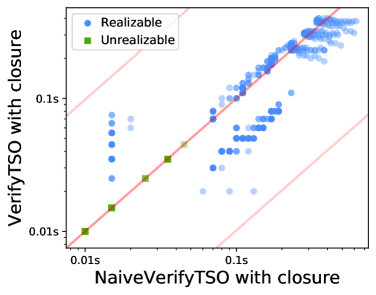
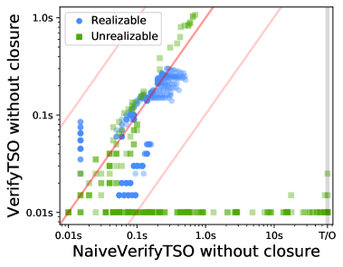
Figure 11. Consistency verification comparison of $\operatorname{VerifyTSO}$ and $\operatorname{NaiveVerifyTSO}$ with closure (left) and without closure (right) on verification instances that contain RMW and CAS instructions.

The results are presented in Figure 11. The left plot depicts the results for $\operatorname{VerifyTSO}$ and $\operatorname{NaiveVerifyTSO}$ when closure is used as a preceding step. Here the results are all within an order-of-magnitude difference, and they are identical for unrealizable instances, since all of them were detected as unrealizable already by the closure. The right plot depicts the results for $\operatorname{VerifyTSO}$ and $\operatorname{NaiveVerifyTSO}$ without using the closure. Here the difference for realizable instances is also within an order of magnitude, but for some unrealizable instances the algorithm $\operatorname{VerifyTSO}$ is significantly faster. Generally, the observed improvement of our $\operatorname{VerifyTSO}$ as compared to $\operatorname{NaiveVerifyTSO}$ is somewhat smaller in Figure 11, which could be due to the fact that executions with RMW and CAS instructions typically have fewer concurrent writes (indeed, in an execution where each write event is a part of a RMW/CAS instruction, each conflicting pair of writes is inherently ordered by the reads-from orderings together with $\mathsf{PO}$). Finally, in Section C.2 the effect of closure is evaluated for both verification algorithms $\operatorname{VerifyTSO}$ and $\operatorname{NaiveVerifyTSO}$ on instances with RMW and CAS.

6.2. Experiments on SMC for TSO and PSO

In this section we focus on assessing the advantages of utilizing the reads-from equivalence for SMC in $\operatorname{TSO}$ and $\operatorname{PSO}$. We have used $\operatorname{RF-SMC}$ for stateless model checking of 109 benchmarks under each memory model $\mathcal{M}\in\{\operatorname{SC},\operatorname{TSO},\operatorname{PSO}\}$, where $\operatorname{SC}$ is handled in our implementation as $\operatorname{TSO}$ with a fence after each thread event. Section C.3 provides further details on our SMC setup.

Comparison.

As a baseline for comparison, we have also executed $\mathsf{Source}$-$\operatorname{DPOR}$ (Abdulla et al., 2014), which is implemented in Nidhugg and explores the trace space using the partitioning based on the Shasha–Snir equivalence. In $\operatorname{SC}$, we have further executed $\mathsf{rfsc}$, the Nidhugg implementation of the reads-from SMC algorithm for $\operatorname{SC}$ by Abdulla et al. (2019), and the full comparison that includes $\mathsf{rfsc}$ for $\operatorname{SC}$ is in Section C.4. Both $\mathsf{rfsc}$ and $\mathsf{Source}$ are well-optimized, and recently started using advanced data-structures for SMC (Lång and Sagonas, 2020). The works of Kokologiannakis et al. (2019b); Kokologiannakis and Vafeiadis (2020) provide a general interface for reads-from SMC in relaxed memory models. However, they handle a given memory model assuming that an auxiliary consistency verification algorithm for that memory model is provided. No such consistency algorithm for $\operatorname{TSO}$ or $\operatorname{PSO}$ is presented by Kokologiannakis et al. (2019b); Kokologiannakis and Vafeiadis (2020), and, to our knowledge, the tool implementations of Kokologiannakis et al. (2019b); Kokologiannakis and Vafeiadis (2020) also lack a consistency algorithm for both $\operatorname{TSO}$ and $\operatorname{PSO}$. Thus these tools are not included in the evaluation.

Evaluation objective.

Our objective for the SMC evaluation is three-fold. First, we want to quantify how each memory model $\mathcal{M}\in\{\operatorname{SC},\operatorname{TSO},\operatorname{PSO}\}$ impacts the size of the RF partitioning. Second, we are interested to see whether, as compared to the baseline Shasha–Snir equivalence, the RF equivalence leads to coarser partitionings for $\operatorname{TSO}$ and $\operatorname{PSO}$, as it does for $\operatorname{SC}$ (Abdulla et al., 2019). Finally, we want to determine whether a coarser RF partitioning leads to faster exploration. Theorem 3.3 states that $\operatorname{RF-SMC}$ spends polynomial time per partitioning class, and we aim to see whether this is a small polynomial in practice.

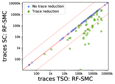
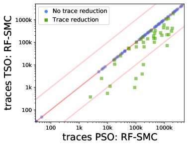
Figure 12. Traces comparison as $\operatorname{RF-SMC}$ moves from $\operatorname{SC}$ to $\operatorname{TSO}$ (left) and from $\operatorname{TSO}$ to $\operatorname{PSO}$ (right).

Results.

We illustrate the obtained results with several scatter plots. Each plot compares two algorithms executing under specified memory models. Then for each benchmark, we consider the highest attempted unroll bound where both the compared algorithms finish before the one-hour timeout. Green dots indicate that a trace reduction was achieved on the underlying benchmark by the algorithm on the y-axis as compared to the algorithm on the x-axis. Benchmarks with no trace reduction are represented by the blue dots. All scatter plots are in log scale, the opaque and semi-transparent red lines represent identity and an order-of-magnitude difference, respectively.

The plots in Figure 12 illustrate how the size of the RF partitioning explored by $\operatorname{RF-SMC}$ changes as we move to more relaxed memory models ($\operatorname{SC}$ to $\operatorname{TSO}$ to $\operatorname{PSO}$). The plots in Figure 13 capture how the size of the RF partitioning explored by $\operatorname{RF-SMC}$ relates to the size of the Shasha–Snir partitioning explored by $\mathsf{Source}$. Finally, the plots in Figure 14 demonstrate the time comparison of $\operatorname{RF-SMC}$ and $\mathsf{Source}$ when there is some (green dots) or no (blue dots) RF-induced trace reduction.

Below we discuss the observations on the obtained results. Table 1 captures detailed results on several benchmarks that we refer to as examples in the discussion.

Figure 13. Traces comparison for $\operatorname{RF-SMC}$ and $\mathsf{Source}$ on the $\operatorname{TSO}$ (left) and $\operatorname{PSO}$ (right) memory model.

Figure 14. Times comparison for $\operatorname{RF-SMC}$ and $\mathsf{Source}$ on the $\operatorname{TSO}$ (left) and $\operatorname{PSO}$ (right) memory model.

Discussion.

We notice that the analysed programs can often exhibit additional behavior in relaxed memory settings. This causes an increase in the size of the partitionings explored by SMC algorithms (see 27_Boop4 in Table 1 as an example). Figure 12 illustrates the overall phenomenon for $\operatorname{RF-SMC}$, where the increase of the RF partitioning size (and hence the number of traces explored) is sometimes beyond an order of magnitude when moving from $\operatorname{SC}$ to $\operatorname{TSO}$, or from $\operatorname{TSO}$ to $\operatorname{PSO}$.

We observe that across all memory models, the reads-from equivalence can offer significant reduction in the trace partitioning as compared to Shasha–Snir equivalence. This leads to fewer traces that need to be explored, see the plots of Figure 13. As we move towards more relaxed memory ($\operatorname{SC}$ to $\operatorname{TSO}$ to $\operatorname{PSO}$), the reduction of RF partitioning often becomes more prominent (see 27_Boop4 in Table 1). Interestingly, in some cases the size of the Shasha–Snir partitioning explored by $\mathsf{Source}$ increases as we move to more relaxed settings, while the RF partitioning remains unchanged (cf. fillarray_false in Table 1). All these observations signify advantages of RF for analysis of the more complex program behavior that arises due to relaxed memory.

We now discuss how trace partitioning coarseness affects execution time, observing the plots of Figure 14. We see that in cases where RF partitioning is coarser (green dots), our RF algorithm $\operatorname{RF-SMC}$ often becomes significantly faster than the Shasha–Snir-based $\mathsf{Source}$, allowing us to analyse programs scaled several levels further (see eratosthenes in Table 1). In cases where the sizes of the RF partitioning and the Shasha–Snir partitioning coincide (blue dots), the well-engineered $\mathsf{Source}$ outperforms our $\operatorname{RF-SMC}$ implementation. The time differences in these cases are reasonably moderate, suggesting that the polynomial overhead incurred to operate on the RF partitioning is small in practice.

Section C.4 contains the complete results on all 109 benchmarks, as well as further scatter plots, illustrating (i) comparison of $\operatorname{RF-SMC}$ with $\mathsf{Source}$ and $\mathsf{rfsc}$ in $\operatorname{SC}$, (ii) time comparison of $\operatorname{RF-SMC}$ across memory models, and (iii) the effect of using closure in the constency checking during SMC.

Benchmark		U	Seq. Consistency		Total Store Order		Partial Store Order
			$\operatorname{RF-SMC}$	$\mathsf{Source}$	$\operatorname{RF-SMC}$	$\mathsf{Source}$	$\operatorname{RF-SMC}$	$\mathsf{Source}$
27_Boop4 threads: 4	Traces	1	2902	21948	3682	36588	8233	572436
		4	197260	3873348	313336	9412428	1807408	-
	Times	1	1.22s	1.74s	1.46s	6.18s	4.40s	169s
		4	124s	550s	182s	2556s	1593s	-
eratosthenes threads: 2	Traces	17	4667	100664	29217	4719488	253125	-
		21	19991	1527736	223929	-	-	-
	Times	17	6.70s	46s	32s	2978s	475s	-
		21	41s	736s	342s	-	-	-
fillarray_false threads: 2	Traces	3	14625	47892	14625	59404	14625	63088
		4	471821	2278732	471821	3023380	471821	3329934
	Times	3	12s	6.18s	12s	12s	18s	39s
		4	553s	331s	547s	778s	930s	2844s

Table 1. SMC results on several benchmarks. U denotes the unroll bound. The timeout of one hour is indicated by “-”. Bold-font entries indicate the smallest numbers for the respective memory model.

7. CONCLUSIONS

In this work we have solved the consistency verification problem under a reads-from map for the $\operatorname{TSO}$ and $\operatorname{PSO}$ relaxed memory models. Our algorithms scale as $O(k\cdot n^{k+1})$ for $\operatorname{TSO}$, and as $O(k\cdot n^{k+1}\cdot\min(n^{k\cdot(k-1)},2^{k\cdot d}))$ for $\operatorname{PSO}$, for $n$ events, $k$ threads and $d$ variables. Thus, they both become polynomial-time for a bounded number of threads, similar to the case for $\operatorname{SC}$ that was established recently (Abdulla et al., 2019; Biswas and Enea, 2019). In practice, our algorithms perform much better than the standard baseline methods, offering significant scalability improvements. Encouraged by these scalability improvements, we have used these algorithms to develop, for the first time, SMC under $\operatorname{TSO}$ and $\operatorname{PSO}$ using the reads-from equivalence, as opposed to the standard Shasha–Snir equivalence. Our experiments show that the underlying reads-from partitioning is often much coarser than the Shasha–Snir partitioning, which yields a significant speedup in the model checking task.

We remark that our consistency-verification algorithms have direct applications beyond SMC. In particular, most predictive dynamic analyses solve a consistency-verification problem in order to infer whether an erroneous execution can be generated by a concurrent system (see, e.g., Smaragdakis et al. (2012); Kini et al. (2017); Mathur et al. (2020)). Hence, the results of this work allow to extend predictive analyses to $\operatorname{TSO}/\operatorname{PSO}$ in a scalable way that does not sacrifice precision. We will pursue this direction in our future work.

Appendix A Details of Section 4

Here we proceed with proofs of our theorems and lemmas regarding algorithms $\operatorname{VerifyTSO}$ and $\operatorname{VerifyPSO}$. Then, we describe an extension of $\operatorname{VerifyPSO}$ to handle store-store fences.

A.1. Proofs of Section 4.1

See 4.1

Proof.

We argue separately about soundness and completeness.

Soundness. We prove by induction that every trace $\sigma$ extracted from $\mathcal{S}$ in Algorithm 1 is a trace that realizes $(X|\mathcal{E}(\sigma),\mathsf{RF}|\mathcal{E}(\sigma))$ under $\operatorname{TSO}$. The claim clearly holds for $\sigma=\epsilon$. Now consider a trace $\sigma$ such that $\sigma\neq\emptyset$, hence $\sigma$ was inserted in $\mathcal{S}$ in Algorithm 1 while executing a previous iteration of the while-loop in Algorithm 1. Let $\sigma^{\prime}$ be the trace that was extracted from $\mathcal{S}$ in that iteration. Observe that $\sigma^{\prime}$ is extended with $\operatorname{TSO}$-executable events in Algorithm 1 and Algorithm 1, hence it is well-formed. It remains to argue that for every new read $\operatorname{r}$ executed in Algorithm 1, we have $\mathsf{RF}_{\sigma^{\prime}}(\operatorname{r})=\mathsf{RF}(\operatorname{r})$. Assume towards contradiction otherwise, and let $\operatorname{r}$ be the first read for which this equality fails. For the remaining of the proof, we let $\sigma^{\prime}$ be the trace in the iteration of Algorithm 1 that executed $\operatorname{r}$, i.e., $\sigma^{\prime}$ ends in $\operatorname{r}$. Let $\mathsf{RF}(\operatorname{r})=(\operatorname{wB},\operatorname{wM})$ and $\mathsf{RF}_{\sigma^{\prime}}(\operatorname{r})=(\operatorname{wB}^{\prime},\operatorname{wM}^{\prime})$. We distinguish the following cases.

1. If $\operatorname{r}$ reads-from $\operatorname{wB}^{\prime}$ in $\sigma^{\prime}$, then $\mathsf{thr}(\operatorname{r})\neq\mathsf{thr}(\operatorname{wB})$, while also $\operatorname{wM}^{\prime}\not\in\mathcal{E}(\sigma)$. Since $\operatorname{r}$ became $\operatorname{TSO}$-executable, we have $\operatorname{wM}\in\mathcal{E}(\sigma^{\prime})$, hence $\operatorname{wM}$ has already become $\operatorname{TSO}$-executable. This violates Item 2b of the definition of $\operatorname{TSO}$-executable memory-writes for $\operatorname{wM}$, a contradiction.

2. If $\operatorname{r}$ reads-from $\operatorname{wM}^{\prime}$ in $\sigma^{\prime}$, then $\operatorname{wM}\in\mathcal{E}(\sigma^{\prime})$ and $\operatorname{wM}^{\prime}$ was executed after $\operatorname{wM}$ was executed in $\sigma^{\prime}$. This violates Item 2a of the definition of $\operatorname{TSO}$-executable memory-writes for $\operatorname{wM}^{\prime}$, a contradiction.

It follows that $\mathsf{RF}_{\sigma^{\prime}}(\operatorname{r})=\mathsf{RF}(\operatorname{r})$ for all reads $\operatorname{r}\in\mathcal{R}(\sigma^{\prime})$, and hence $\sigma^{\prime}$ realizes $(X|\mathcal{E}(\sigma^{\prime}),\mathsf{RF}|\mathcal{E}(\sigma^{\prime}))$ under $\operatorname{TSO}$. The above soundness argument carries over to executions containing RMW and CAS instructions, since (i) such instructions are modeled by events of already considered types (c.f. Section 4.4), while respecting the $\operatorname{TSO}$-executability requirements of these events (as were defined in Section 4.1), and (ii) in Algorithm 1 resp. Algorithm 1 we only consider $\operatorname{TSO}$-executable atomic blocks (described in detail in Section 4.4).

Completeness. Consider any trace $\sigma^{*}$ that realizes $(X,\mathsf{RF})$. We show by induction that for every prefix $\overline{\sigma}$ of $\sigma^{*}$, the algorithm examines a trace $\sigma$ in Algorithm 1 such that (i) $\mathcal{W}^{M}(\overline{\sigma})=\mathcal{W}^{M}(\sigma)$, and (ii) $\mathcal{L}(\overline{\sigma})\subseteq\mathcal{L}(\sigma)$. The proof is by induction on the number of memory-writes of $\overline{\sigma}$. Let $\overline{\sigma}=\overline{\sigma}^{\prime}\circ\kappa\circ\operatorname{wM}$, where $\kappa$ is a sequence of thread events. Assume by the induction hypothesis that the algorithm extracts a trace $\sigma^{\prime}$ in Algorithm 1 such that (i) $\mathcal{W}^{M}(\overline{\sigma}^{\prime})=\mathcal{W}^{M}(\sigma^{\prime})$, and (ii) $\mathcal{L}(\overline{\sigma^{\prime}})\subseteq\mathcal{L}(\sigma^{\prime})$. (note that the statement clearly holds for the base case where $\overline{\sigma}^{\prime}=\epsilon$). By a straightforward induction, all the events of $\kappa$ not already present in $\sigma^{\prime}$ become eventually $\operatorname{TSO}$-executable in $\sigma^{\prime}$, and thus appended in $\sigma^{\prime}$, as the algorithm executes the while-loop in Algorithm 1. Hence, at the end of this while-loop, we have (i) $\mathcal{W}^{M}(\overline{\sigma}^{\prime})=\mathcal{W}^{M}(\sigma^{\prime})$, and (ii) $\mathcal{L}(\overline{\sigma}^{\prime})\cup\mathcal{E}(\kappa)\subseteq\mathcal{L}(\sigma^{\prime})$.

It remains to argue that $\operatorname{wM}$ is $\operatorname{TSO}$-executable in $\sigma^{\prime}$ at this point (i.e., in Algorithm 1). Assume towards contradiction otherwise, hence one of the following hold.

1. There is a read $\operatorname{r}\in\mathcal{R}(X)$ with $\mathsf{RF}(\operatorname{r})=(\operatorname{wB}^{\prime},\operatorname{wM}^{\prime})$ and such that (i) $\operatorname{r}\Join\operatorname{wM}$, (ii) $\operatorname{wM}\neq\operatorname{wM}^{\prime}$, (iii) $\operatorname{wM}^{\prime}\in\sigma^{\prime}$, and (iv) $\operatorname{r}\not\in\sigma^{\prime}$. By the induction hypothesis, we have $\mathcal{W}^{M}(\sigma^{\prime})=\mathcal{W}^{M}(\overline{\sigma}^{\prime})$ and thus $\operatorname{wM}^{\prime}\in\overline{\sigma}^{\prime}$. Moreover, we have $\mathcal{E}(\overline{\sigma}^{\prime}\circ\kappa)\subseteq\mathcal{E}(\sigma^{\prime})$, and thus $\operatorname{r}\not\in\overline{\sigma}^{\prime}\circ\kappa$. This violates the fact that $\overline{\sigma}$ is a witness prefix for $(X,\mathsf{RF})$.

2. There is a read $\operatorname{r}\in\mathcal{R}(X)$ with $\mathsf{RF}(\operatorname{r})=(\operatorname{wB},\operatorname{wM})$ and such that there exists a two-phase write $(\operatorname{wB}^{\prime},\operatorname{wM}^{\prime})$ with (i) $\operatorname{r}\Join\operatorname{wB}^{\prime}$, (ii) $\operatorname{wB}^{\prime}<_{\mathsf{PO}}\operatorname{r}$, (iii) $\operatorname{wM}^{\prime}\not\in\sigma^{\prime}$. By the induction hypothesis, we have $\mathcal{W}^{M}(\sigma^{\prime})=\mathcal{W}^{M}(\overline{\sigma}^{\prime})$ and thus $\operatorname{wM}^{\prime}\not\in\overline{\sigma}^{\prime}$. Moreover, we have $\mathcal{E}(\overline{\sigma}^{\prime}\circ\kappa)\subseteq\mathcal{E}(\sigma^{\prime})$, and thus $\operatorname{r}\not\in\overline{\sigma}^{\prime}\circ\kappa$. This violates the fact that $\overline{\sigma}$ is a witness prefix for $(X,\mathsf{RF})$.

Hence $\operatorname{wM}$ is $\operatorname{TSO}$-executable in $\sigma^{\prime}$ in Algorithm 1, and thus the algorithm will construct the trace $\sigma^{\prime}_{\operatorname{wM}}=\sigma^{\prime}\circ\operatorname{wM}$ in Algorithm 1. If $\mathcal{W}^{M}(\sigma^{\prime}_{\operatorname{wM}})\not\in\mathsf{Done}$, the test in Algorithm 1 succeeds, and the statement holds for $\sigma$ being $\sigma^{\prime}_{\operatorname{wM}}$ extracted from $\mathcal{S}$ in a later iteration. Otherwise, the algorithm previously constructed a trace $\sigma^{\prime\prime}$ with $\mathcal{W}^{M}(\sigma^{\prime\prime})=\mathcal{W}^{M}(\sigma^{\prime}_{\operatorname{wM}})$, and the statement holds for $\sigma$ being $\sigma^{\prime\prime}$ extracted from $\mathcal{S}$ in a later iteration.

When arguing about completeness in the presence of RMW and CAS instructions, additional care needs to be taken, as follows. The above induction argument applies, but it needs to additionally consider a case with $\overline{\sigma}=\overline{\sigma}^{\prime}\circ\kappa\circ\operatorname{r}\circ\operatorname{wB}\circ\operatorname{wM}$ and $\operatorname{fnc}\in\mathcal{E}(\overline{\sigma}^{\prime}\circ\kappa)$, where $\operatorname{fnc}$ together with $\operatorname{r}\circ\operatorname{wB}\circ\operatorname{wM}$ represent an atomic RMW resp. CAS instruction with the write-part designated to be immediately propagated to the shared memory. Let us consider this case in what follows.

As above, we start with the induction hypothesis that in Algorithm 1 we have $\sigma^{\prime}$ with (i) $\mathcal{W}^{M}(\overline{\sigma}^{\prime})=\mathcal{W}^{M}(\sigma^{\prime})$, and (ii) $\mathcal{L}(\overline{\sigma^{\prime}})\subseteq\mathcal{L}(\sigma^{\prime})$. Further, by an argument similar to the above, we reach Algorithm 1 where $\sigma^{\prime}$ now satisfies (i) $\mathcal{W}^{M}(\overline{\sigma}^{\prime})=\mathcal{W}^{M}(\sigma^{\prime})$, and (ii) $\mathcal{L}(\overline{\sigma}^{\prime})\cup\mathcal{E}(\kappa)\subseteq\mathcal{L}(\sigma^{\prime})$. At this point, we have $\operatorname{fnc}\in\mathcal{E}(\overline{\sigma}^{\prime}\circ\kappa)$ and $\operatorname{fnc}\in\mathcal{L}(\sigma^{\prime})$. Further, since in our approach we emplace $\operatorname{r}$, $\operatorname{wB}$ and $\operatorname{wM}$ in an atomic block, and we never allow execution of a singular event that is part of some atomic block (described in detail in Section 4.4), we have that $\mathcal{E}(\sigma^{\prime})\cap\{\operatorname{r},\operatorname{wB},\operatorname{wM}\}=\emptyset$. As a result, since there are no events between $\operatorname{fnc}$ and $\operatorname{r}$ in the thread of the atomic instruction, we have that the buffer of the thread of the atomic instruction is empty in both $\overline{\sigma}^{\prime}\circ\kappa$ and $\sigma^{\prime}$. What remains to argue is that the atomic block $\operatorname{r}\circ\operatorname{wB}\circ\operatorname{wM}$ is $\operatorname{TSO}$-executable in $\sigma^{\prime}$. For this, we refer to the $\operatorname{TSO}$-executable conditions of atomic blocks defined in Section 4.4. In turn, utilizing the $\operatorname{TSO}$-executable conditions of (i) reads, (ii) buffer-writes, and (iii) memory-writes, defined in Section 4.1, we show that (i) $\operatorname{r}$ is $\operatorname{TSO}$-executable in $\sigma^{\prime}$, (ii) $\operatorname{wB}$ is $\operatorname{TSO}$-executable in $\sigma^{\prime}\circ\operatorname{r}$, and (iii) $\operatorname{wM}$ is $\operatorname{TSO}$-executable in $\sigma^{\prime}\circ\operatorname{r}\circ\operatorname{wB}$. This together with $\mathcal{E}(\sigma^{\prime})\cap\{\operatorname{r},\operatorname{wB},\operatorname{wM}\}=\emptyset$ gives us that the atomic block $\operatorname{r}\circ\operatorname{wB}\circ\operatorname{wM}$ is $\operatorname{TSO}$-executable in $\sigma^{\prime}$, and thus in Algorithm 1 the algorithm will construct the trace $\sigma^{\prime\prime}=\sigma^{\prime}\circ\operatorname{r}\circ\operatorname{wB}\circ\operatorname{wM}$.

The desired completeness result follows. ∎

We conclude the section with the proof of Theorem 3.1.

See 3.1

Proof.

Lemma 4.1 establishes the correctness, so here we focus on the complexity, and the following argument applies also to executions containing RMW and CAS instructions.

Since there are $k$ threads, there exist at most $n^{k}$ distinct traces $\sigma_{1},\sigma_{2}$ with $\mathcal{W}^{M}(\sigma_{1})\neq\mathcal{W}^{M}(\sigma_{2})$. Hence, the main loop in Algorithm 1 is executed at most $n^{k}$ times. For each of the $\leq n^{k}$ traces $\sigma$ inserted in $\mathcal{S}$ in Algorithm 1, there exist at most $k-1$ traces that are not inserted in $\mathcal{S}$ because $\mathcal{W}^{M}(\sigma)=\mathcal{W}^{M}(\sigma^{\prime})$ (hence the test in Algorithm 1 fails). Hence, the algorithm handles $O(k\cdot n^{k})$ traces in total, while each trace is constructed in $O(n)$ time. Thus, the complexity of $\operatorname{VerifyTSO}$ is $O(k\cdot n^{k+1})$. The desired result follows. ∎

A.2. Proofs of Section 4.2

See 4.2

Proof.

Since $\operatorname{wM}$ is executable in $\sigma_{1}$, the variable $\mathsf{var}(\sigma_{1})$ is not held in $\sigma_{1}$. It follows directly from the definition of fence maps that the read sets $A_{\mathsf{thr},\mathsf{thr}^{\prime}}$ can only increase in $\operatorname{FMap}_{\sigma_{2}}$ compared to $\operatorname{FMap}_{\sigma_{1}}$. Hence, $\operatorname{FMap}_{\sigma_{1}}(\mathsf{thr}_{1},\mathsf{thr}_{2})\leq\operatorname{FMap}_{\sigma_{2}}(\mathsf{thr}_{1},\mathsf{thr}_{2})$ for all $\mathsf{thr}_{1},\mathsf{thr}_{2}$. Moreover, if $\operatorname{wM}$ is spurious then the sets $A_{\mathsf{thr},\mathsf{thr}^{\prime}}$ are identical, thus $\operatorname{FMap}_{\sigma_{1}}(\mathsf{thr}_{1},\mathsf{thr}_{2})=\operatorname{FMap}_{\sigma_{2}}(\mathsf{thr}_{1},\mathsf{thr}_{2})$ for all $\mathsf{thr}_{1},\mathsf{thr}_{2}$.

The desired result follows. ∎

See 4.3

Proof.

We distinguish cases based on the type of $e$.

1. If $e$ is a fence $\operatorname{fnc}$, the fence maps do not chance, hence the claim holds directly from the fact that $\operatorname{FMap}_{\sigma_{1}}\leq\operatorname{FMap}_{\sigma_{2}}$.

2. If $e$ is a read $\operatorname{r}$, observe that $\operatorname{FMap}_{\sigma^{\prime}_{i}}\leq\operatorname{FMap}_{\sigma_{i}}$ for each $i\in[2]$. Hence we must have $\operatorname{FMap}_{\sigma^{\prime}_{2}}(\mathsf{thr}_{1},\mathsf{thr}_{2})<\operatorname{FMap}_{\sigma_{2}}(\mathsf{thr}_{1},\mathsf{thr}_{2})$, for some thread $\mathsf{thr}_{1}\in\operatorname{Threads}$ and $\mathsf{thr}_{2}=\mathsf{thr}(\operatorname{r})$. Note that in fact $\operatorname{FMap}_{\sigma^{\prime}_{2}}(\mathsf{thr}_{1},\mathsf{thr}_{2})=0$, which occurs because $\operatorname{FMap}_{\sigma_{2}}(\mathsf{thr}_{1},\mathsf{thr}_{2})$ is the index of $\operatorname{r}$ in $\mathsf{thr}_{2}$. Since $\operatorname{FMap}_{\sigma_{1}}\leq\operatorname{FMap}_{\sigma_{2}}$, we have either $\operatorname{FMap}_{\sigma_{1}}(\mathsf{thr}_{1},\mathsf{thr}_{2})=0$ or $\operatorname{FMap}_{\sigma_{1}}(\mathsf{thr}_{1},\mathsf{thr}_{2})=\operatorname{FMap}_{\sigma_{2}}(\mathsf{thr}_{1},\mathsf{thr}_{2})$. In either case, we have $\operatorname{FMap}_{\sigma^{\prime}_{1}}\leq\operatorname{FMap}_{\sigma_{2}}=0$, a contradiction.

3. If $e$ is a buffer-write $\operatorname{wB}$, observe that $\operatorname{FMap}_{\sigma_{i}}\leq\operatorname{FMap}_{\sigma^{\prime}_{i}}$ for each $i\in[2]$. Hence we must have $\operatorname{FMap}_{\sigma_{1}}(\mathsf{thr}_{1},\mathsf{thr}_{2})<\operatorname{FMap}_{\sigma^{\prime}_{1}}(\mathsf{thr}_{1},\mathsf{thr}_{2})$, where $\mathsf{thr}_{1}=\mathsf{thr}(\operatorname{wB})$ and $\mathsf{thr}_{2}$ is some other thread. It follows that $v=\mathsf{var}(\operatorname{wB})$ is held in $\sigma_{1}$ by an active memory-write $\operatorname{wM}^{\prime}$ (thus $\operatorname{wM}^{\prime}$ is not spurious in $\sigma_{1}$), and $\operatorname{FMap}_{\sigma^{\prime}_{1}}(\mathsf{thr}_{1},\mathsf{thr}_{2})$ is the index of $\mathsf{thr}_{2}$ that contains a read $\operatorname{r}$ with $\mathsf{RF}(\operatorname{r})=(\_,\operatorname{wM}^{\prime})$. Since $\mathcal{W}^{M}(\sigma_{1})\setminus\mathcal{SW}^{M}(\sigma_{1})\subseteq\mathcal{W}^{M}(\sigma_{2})$, we have $\mathcal{W}^{M}(^{\prime})\in\sigma_{2}$ Since $\mathcal{L}(\sigma_{1})=\mathcal{L}(\sigma_{2})$, we have that $\operatorname{wM}^{\prime}$ is an active memory-write in $\sigma_{2}$. Hence $\operatorname{FMap}_{\sigma^{\prime}_{2}}(\mathsf{thr}_{1},\mathsf{thr}_{2})\geq\operatorname{FMap}_{\sigma^{\prime}_{1}}(\mathsf{thr}_{1},\mathsf{thr}_{2})$, a contradiction.

The desired result follows. ∎

See 4.4

Proof.

Given a trace $\sigma$, we define the non-empty-buffer map $\operatorname{NEBMap}_{\sigma}\colon\operatorname{Threads}\times\mathcal{G}\to\{\mathsf{True},\mathsf{False}\}$, such that $\operatorname{NEBMap}_{\sigma}(\mathsf{thr},v)=\mathsf{True}$ iff (i) $\mathsf{thr}$ does not hold variable $v$, and (ii) the buffer of thread $\mathsf{thr}$ on variable $v$ is non-empty. Clearly there exist at most $2^{k\cdot d}$ different non-empty-buffer maps. We argue that for every two traces $\sigma_{1},\sigma_{2}$, if $\mathcal{L}(\sigma_{1})=\mathcal{L}(\sigma_{2})$ and $\operatorname{NEBMap}_{\sigma_{1}}=\operatorname{NEBMap}_{\sigma_{2}}$ then $\operatorname{FMap}_{\sigma_{1}}=\operatorname{FMap}_{\sigma_{2}}$, from which the $2^{k\cdot d}$ bound of the lemma follows.

Assume towards contradiction that $\operatorname{FMap}_{\sigma_{1}}\neq\operatorname{FMap}_{\sigma_{2}}$. Hence, wlog, there exist two threads $\mathsf{thr}_{1},\mathsf{thr}_{2}$ such that $\operatorname{FMap}_{\sigma_{2}}(\mathsf{thr}_{1},\mathsf{thr}_{2})>\operatorname{FMap}_{\sigma_{1}}(\mathsf{thr}_{1},\mathsf{thr}_{2})$. Let $\operatorname{FMap}_{\sigma_{2}}(\mathsf{thr}_{1},\mathsf{thr}_{2})=m$, and consider the read $\operatorname{r}$ of $\mathsf{thr}_{2}$ at index $m$. Let $v=\mathsf{var}(\operatorname{r})$ and $\mathsf{RF}(\operatorname{r})=(\operatorname{wB},\operatorname{wM})$ and $\mathsf{thr}_{3}=\mathsf{thr}(\operatorname{wB})$. By the definition of fence maps, we have that $\mathsf{thr}_{3}$ holds variable $v$ in $\sigma_{2}$. By the definition of non-empty-buffer maps, we have that $\operatorname{NEBMap}_{\sigma_{2}}(\mathsf{thr}_{3},v)=\mathsf{False}$, and since $\operatorname{NEBMap}_{\sigma_{1}}=\operatorname{NEBMap}_{\sigma_{2}}$, we also have $\operatorname{NEBMap}_{\sigma_{1}}(\mathsf{thr}_{3},v)=\mathsf{False}$. Since $\mathcal{L}(\sigma_{1})=\mathcal{L}(\sigma_{2})$, we have that $\operatorname{wB}\in\sigma_{1}$. Moreover, we have $\operatorname{wM}\not\in\sigma_{1}$, as otherwise, since $\operatorname{NEBMap}_{\sigma_{1}}(\mathsf{thr}_{1})=\operatorname{NEBMap}_{\sigma_{1}}(\mathsf{thr}_{2})$, we would have $\operatorname{FMap}_{\sigma_{1}}(\mathsf{thr}_{1},\mathsf{thr}_{2})\geq m$. Hence, the buffer of thread $\mathsf{thr}_{3}$ on variable $v$ is non-empty in $\sigma_{1}$. Since $\operatorname{NEBMap}_{\sigma_{1}}(\mathsf{thr}_{3},v)=\mathsf{False}$, we have that $\mathsf{thr}_{3}$ holds $v$ in $\sigma_{1}$. Thus, there is a read $\operatorname{r}^{\prime}\not\in\sigma_{1}$ with $\mathsf{RF}(\operatorname{r}^{\prime})=(\operatorname{wB}^{\prime},\operatorname{wM}^{\prime})$, where $\operatorname{wM}^{\prime}<_{\mathsf{PO}}\operatorname{wM}$. Since $\mathcal{L}(\sigma_{1})=\mathcal{L}(\sigma_{2})$, we have that $\operatorname{r}^{\prime}\not\in\sigma_{2}$, which violates the observation of $\operatorname{r}^{\prime}$ in any extension of $\sigma_{2}$.

The desired result follows. ∎

See 4.5

Proof.

We argue separately about soundness and completeness.

Soundness. We prove by induction that every trace $\sigma$ extracted from $\mathcal{S}$ in Algorithm 2 is a trace that realizes $(X|\mathcal{E}(\sigma),\mathsf{RF}|\mathcal{E}(\sigma))$ under $\operatorname{PSO}$. The claim clearly holds for $\sigma=\epsilon$. Now consider a trace $\sigma$ such that $\sigma\neq\emptyset$, hence $\sigma$ was inserted in $\mathcal{S}$ in Algorithm 2 while executing a previous iteration of the while-loop in Algorithm 2. Let $\sigma^{\prime}$ be the trace that was extracted from $\mathcal{S}$ in that iteration, and consider the trace $\sigma_{e}$ constructed in Algorithm 2. Since $\sigma_{e}$ is obtained by extending $\sigma^{\prime}$ with $\operatorname{PSO}$-executable events, it follows that $\sigma_{e}$ is well-formed. It remains to argue that $\mathsf{RF}_{\sigma}\subseteq\mathsf{RF}$. If $e$ is not a read, then the claim holds by the induction hypothesis as $\mathcal{R}(\sigma_{e})=\mathcal{R}(\sigma^{\prime})$. Now assume that $e$ is a read with $\mathsf{RF}_{\sigma_{e}}(e)=(\operatorname{wB}^{\prime},\operatorname{wM}^{\prime})$. Let $\mathsf{RF}(e)=(\operatorname{wB},\operatorname{wM})$, and assume towards contradiction that $\operatorname{wB}\neq\operatorname{wB}$. We distinguish the following cases.

1. If $e$ reads-from $\operatorname{wB}^{\prime}$ in $\sigma_{e}$, we have that $\mathsf{thr}(\operatorname{r})\neq\mathsf{thr}(\operatorname{wB})$. But then $\operatorname{wM}\in\sigma_{e}$, hence $\operatorname{wM}$ has become $\operatorname{PSO}$-executable, and thus $\operatorname{wM}^{\prime}\in\sigma_{e}$. Since $e$ is the last event of $\sigma_{e}$ this violates the fact that $e$ reads-from $\operatorname{wB}^{\prime}$ in $\sigma_{e}$.

2. If $e$ reads-from $\operatorname{wM}^{\prime}$ in $\sigma_{e}$, then $\operatorname{wM}\in\sigma^{\prime}$, and $\operatorname{wM}^{\prime}$ was executed after $\operatorname{wM}$ in $\sigma^{\prime}$. By the definition of $\operatorname{PSO}$-executable events, $\operatorname{wM}^{\prime}$ could not have been $\operatorname{PSO}$-executable at that point, a contradiction.

It follows that $\mathsf{RF}_{\sigma_{e}}(e)=\mathsf{RF}(e)$, and this with the induction hypothesis gives us that $\mathsf{RF}_{\sigma_{e}}(\operatorname{r})=\mathsf{RF}(\operatorname{r})$ for all reads $\operatorname{r}\in\mathcal{R}(\sigma_{e})$. As a result, $\sigma_{e}$ realizes $(X|\mathcal{E}(\sigma_{e}),\mathsf{RF}|\mathcal{E}(\sigma_{e}))$ under $\operatorname{PSO}$. The soundness argument carries over directly to executions containing RMW and CAS instructions. Indeed, since in Algorithm 2 we only consider atomic blocks that are $\operatorname{PSO}$-executable (described in Section 4.4), consequently, the $\operatorname{PSO}$-executable conditions of fences, reads, buffer-writes and memory-writes (as defined in Section 4.2) used to model RMW and CAS are preserved, which by the above argument implies soundness.

Completeness. Consider any trace $\sigma^{*}$ that realizes $(X,\mathsf{RF})$. We show by induction that for every prefix $\overline{\sigma}$ of $\sigma^{*}$, the algorithm examines a trace $\sigma$ in Algorithm 2 such that (i) $\mathcal{L}(\sigma)=\mathcal{L}(\overline{\sigma})$, (ii) $\mathcal{W}^{M}(\sigma)\setminus\mathcal{SW}^{M}(\sigma)\subseteq\mathcal{W}^{M}(\overline{\sigma})$, and (iii) $\operatorname{FMap}_{\sigma}\leq\operatorname{FMap}_{\overline{\sigma}}$.

The proof is by induction on the number of thread events of $\overline{\sigma}$. The statement clearly holds when $\overline{\sigma}=\epsilon$ due to the initialization of $\mathcal{S}$. For the inductive step, let $\overline{\sigma}=\overline{\sigma}^{\prime}\circ\kappa\circ e$, where $\kappa$ is a sequence of memory-writes and $e$ is a thread event. By the induction hypothesis, the algorithm extracts a trace $\sigma^{\prime}$ in Algorithm 2 such that (i) $\mathcal{L}(\sigma^{\prime})=\mathcal{L}(\overline{\sigma}^{\prime})$, (ii) $\mathcal{W}^{M}(\sigma^{\prime})\setminus\mathcal{SW}^{M}(\sigma^{\prime})\subseteq\mathcal{W}^{M}(\overline{\sigma}^{\prime})$, (iii) $\operatorname{FMap}_{\sigma^{\prime}}\leq\operatorname{FMap}_{\overline{\sigma}^{\prime}}$. Let $\overline{\sigma}_{1}=\overline{\sigma}^{\prime}\circ\kappa$, and $\sigma_{1}$ be the trace $\sigma^{\prime}$ after the algorithm has extended $\sigma^{\prime}$ with all events in the while-loop of Algorithm 2. By Lemma 4.2, we have $\operatorname{FMap}_{\overline{\sigma}^{\prime}}\leq\operatorname{FMap}_{\overline{\sigma}_{1}}$. Since all events appended to $\sigma^{\prime}$ are spurious memory-writes in $\sigma^{\prime}$, by Lemma 4.2, we have $\operatorname{FMap}_{\sigma_{1}}=\operatorname{FMap}_{\sigma^{\prime}}$ and thus $\operatorname{FMap}_{\sigma_{1}}\leq\operatorname{FMap}_{\overline{\sigma}_{1}}$. Moreover, since the while-loop only appends spurious memory-writes to $\sigma^{\prime}$, we have $\mathcal{W}^{M}(\sigma_{1})\setminus\mathcal{SW}^{M}(\sigma_{1})\subseteq\mathcal{W}^{M}(\overline{\sigma}_{1})$. Finally, we trivially have $\mathcal{L}(\sigma_{1})=\mathcal{L}(\overline{\sigma}_{1})$.

We now argue that $e$ is $\operatorname{PSO}$-executable in $\sigma_{1}$ in Algorithm 2, and the statement holds for the new trace $\sigma_{e}$ constructed in Algorithm 2. We distinguish cases based on the type of $e$.

1. If $e$ is a buffer-write, then $\mathcal{E}(\sigma_{1})\cup\{e\}$ is a lower set of $(X,\mathsf{RF})$, hence $e$ is $\operatorname{PSO}$-executable in $\sigma_{1}$. Thus, we have $\mathcal{L}(\overline{\sigma})=\mathcal{L}(\sigma_{e})$. Moreover, note that $\sigma_{e}=\sigma_{1}\circ e$ and $\overline{\sigma}=\overline{\sigma}_{1}\circ e$. By Lemma 4.3 on $\sigma_{1}$ and $\overline{\sigma}_{1}$, we have $\operatorname{FMap}_{\sigma_{e}}\leq\operatorname{FMap}_{\overline{\sigma}}$. Finally, we have $\mathcal{W}^{M}(\sigma_{e})=\mathcal{W}^{M}(\sigma_{1})$ and thus $\mathcal{W}^{M}(\sigma_{e})\setminus\mathcal{SW}^{M}(\sigma_{e})\subseteq\mathcal{W}^{M}(\overline{\sigma})$.

2. If $e$ is a read, let $\mathsf{RF}(e)=(\operatorname{wB},\operatorname{wM})$ and $v=\mathsf{var}(e)$. We have $\operatorname{wB}\in\overline{\sigma}_{1}$ and thus $\operatorname{wB}\in\sigma_{1}$. If $\mathsf{thr}(\operatorname{wB})=\mathsf{thr}(e)$, then $e$ is $\operatorname{PSO}$-executable in $\sigma_{1}$. Now consider that $\mathsf{thr}(\operatorname{wB})\neq\mathsf{thr}(e)$, and assume towards contradiction that $e$ is not $\operatorname{PSO}$-executable in $\sigma_{1}$. There are two cases where this can happen.

   The first case is when the variable $v$ is held by another memory write in $\sigma_{1}$. Since $\mathcal{L}(\sigma_{1})=\mathcal{L}(\overline{\sigma}_{1})$ and $\mathcal{W}^{M}(\sigma_{1})\setminus\mathcal{SW}^{M}(\sigma_{1})\subseteq\mathcal{W}^{M}(\overline{\sigma}_{1})$, the variable $v$ is also held by another memory write in $\overline{\sigma}_{1}$, and thus $\operatorname{wM}$ is neither in $\overline{\sigma}_{1}$ nor $\operatorname{PSO}$-executable in $\overline{\sigma}_{1}$. Thus $e$ is not $\operatorname{PSO}$-executable in $\overline{\sigma}_{1}$ either, a contradiction.

   The second case is when there exists a read $\operatorname{r}\not\in\sigma_{1}$ such that $\mathsf{RF}(\operatorname{r})=(\_,\operatorname{wM})$, and there exists a local write event $w^{\prime}=(\operatorname{wB}^{\prime},\operatorname{wM}^{\prime})$ with $\mathsf{thr}(\operatorname{wB}^{\prime})=\mathsf{thr}(\operatorname{r})$ but $\operatorname{wM}^{\prime}\not\in\sigma_{1}$. Since $\overline{\sigma}_{1}$ is a witness prefix, we have $\operatorname{wM}^{\prime}\in\overline{\sigma}_{1}$, hence $\operatorname{wB}^{\prime}\in\overline{\sigma}_{1}$, and since $\mathcal{L}(\sigma_{1})=\mathcal{L}(\overline{\sigma}_{1})$, we also have $\operatorname{wB}^{\prime}\in\sigma_{1}$. Thus $\operatorname{wM}^{\prime}$ is a pending memory write for the thread $\mathsf{thr}^{\prime}=\mathsf{thr}(\operatorname{wM}^{\prime})$. Let $\operatorname{wM}^{\prime\prime}$ be the earliest (wrt $\mathsf{PO}$) pending memory-write of $\mathsf{thr}^{\prime}$ for the variable $v$. Thus $\operatorname{wM}^{\prime\prime}<_{\mathsf{PO}}\operatorname{wM}^{\prime}$, and hence $\operatorname{wM}^{\prime\prime}\in\overline{\sigma}_{1}$. Note that $\operatorname{wM}^{\prime\prime}$ is not read-from by any read not in $\sigma_{1}$, and hence $\operatorname{wM}^{\prime\prime}$ is spurious in $\sigma_{1}$. But then, the while loop in Algorithm 2 must have added $\operatorname{wM}^{\prime\prime}$ in $\sigma_{1}$, a contradiction.

   It follows that $e$ is $\operatorname{PSO}$-executable in $\sigma_{1}$, and thus $\mathcal{L}(\overline{\sigma})=\mathcal{L}(\sigma_{e})$. Let $\sigma_{2}=\sigma_{1}$ if $\operatorname{wM}\in\sigma_{1}$, else $\sigma_{2}=\sigma_{1}\circ\operatorname{wM}$. Observe that if $\operatorname{wM}$ is $\operatorname{PSO}$-executable in $\sigma_{1}$, all pending memory-writes $\operatorname{wM}^{\prime}$ on variable $v$ of threads other than $\mathsf{thr}(\operatorname{wB})$ are spurious in $\sigma^{\prime}$, and thus all such buffers are empty in $\sigma_{1}$. It follows that $\operatorname{FMap}_{\sigma_{2}}\leq\operatorname{FMap}_{\sigma_{1}}$ and thus $\operatorname{FMap}_{\sigma_{2}}\leq\operatorname{FMap}_{\overline{\sigma}_{1}}$. Moreover, trivially $\mathcal{W}^{M}(\sigma_{2})\setminus\mathcal{SW}^{M}(\sigma_{2})\subseteq\overline{\sigma_{1}}$. Finally, executing $e$ in $\sigma_{2}$ and $\overline{\sigma}_{1}$, we obtain respectively $\sigma_{e}$ and $\overline{\sigma}$, and by Lemma 4.3, we have $\operatorname{FMap}_{\sigma_{e}}\leq\operatorname{FMap}_{\overline{\sigma}}$. Moreover, clearly $\mathcal{W}^{M}(\sigma_{e})=\mathcal{W}^{M}(\sigma_{2})$ and thus $\mathcal{W}^{M}(\sigma_{e})\setminus\mathcal{SW}^{M}(\sigma_{e})\subseteq\overline{\sigma}$.

3. If $e$ is a fence, let $\mu=\operatorname{wM}_{1},\dots,\operatorname{wM}_{j}$ be the sequence of pending memory-writes constructed in Algorithm 2. By a similar analysis to the case where $e$ is a a read event, we have that $\mu$ contains at most one memory-write per variable, as all preceding ones (wrt $\mathsf{PO}$) must be spurious. Assume towards contradiction that some pending memory write $\operatorname{wM}_{i}$ is not $\operatorname{PSO}$-executable in $\sigma$, and let $v=\mathsf{var}(\operatorname{wM}_{i})$. There are two cases to consider.

   1. $\operatorname{wM}_{i}$ is not $\operatorname{PSO}$-executable because $v$ is held in $\sigma_{1}$. Let $\operatorname{wM}$ be the memory-write that holds $v$ in $\sigma_{1}$, and $\operatorname{r}$ be the corresponding read with $\mathsf{RF}(\operatorname{r})=(\_,\operatorname{wM})$ and $\operatorname{r}\not\in\sigma_{1}$. Since $\mathcal{L}(\sigma_{1})=\mathcal{L}(\overline{\sigma}_{1})$, we have $\operatorname{r}\not\in\overline{\sigma}_{1}$. Let $\mathsf{thr}_{1}=\mathsf{thr}(e)$, $\mathsf{thr}_{2}=\mathsf{thr}(\operatorname{r})$, and $m$ be the index of $\operatorname{r}$ in $\mathsf{thr}_{2}$. We have $\operatorname{FMap}_{\sigma_{1}}(\mathsf{thr}_{1},\mathsf{thr}_{2})\geq m$, and since $\operatorname{FMap}_{\sigma_{1}}\leq\operatorname{FMap}_{\overline{\sigma}^{\prime}}$, we also have $\operatorname{FMap}_{\overline{\sigma}^{\prime}}(\mathsf{thr}_{1},\mathsf{thr}_{2})\geq m$. But then there is a pending memory-write $\operatorname{wM}^{\prime}\in\overline{\sigma}^{\prime}$ with $\mathsf{thr}(\operatorname{wM}^{\prime})=\mathsf{thr}_{1}$ and $\operatorname{wM}^{\prime}\not\in\overline{\sigma}_{1}$. Hence $e$ is not $\operatorname{PSO}$-executable in $\overline{\sigma}_{1}$, a contradiction.

   2. $\operatorname{wM}_{i}$ is not $\operatorname{PSO}$-executable because there exists a read $\operatorname{r}\not\in\sigma_{1}$ such that $\mathsf{RF}(\operatorname{r})=(\_,\operatorname{wM}_{i})$, and there exists a local write event $w=(\operatorname{wB},\operatorname{wM})$ with $\mathsf{thr}(\operatorname{wB})=\mathsf{thr}(\operatorname{r})$ but $\operatorname{wM}\not\in\sigma_{1}$. The analysis is similar to the case of $e$ being a read, which leads to a contradiction.

   Thus, we have that the fence $e$ is $\operatorname{PSO}$-executable in $\sigma_{1}$. It is straightforward to see that $\mathcal{W}^{M}(\sigma_{e})\setminus\mathcal{SW}^{M}(\sigma_{e})\subseteq\overline{\sigma}$, and thus it remains to argue that $\operatorname{FMap}_{\sigma_{e}}\leq\operatorname{FMap}_{\overline{\sigma}}$. Let $\sigma_{1}^{j}=\sigma_{1}\circ\operatorname{wM}_{1},\dots,\operatorname{wM}_{j-1}$. It suffices to argue that $\operatorname{FMap}_{\sigma_{1}^{j+1}}\leq\operatorname{FMap}_{\overline{\sigma}_{1}}$, as $\sigma_{e}=\sigma_{1}^{j+1}\circ e$ and $\overline{\sigma}=\overline{\sigma}_{1}\circ e$, and the claim holds by Lemma 4.3 on $\sigma_{1}^{j+1}$ and $\overline{\sigma}_{1}$. The proof is by induction on $\sigma_{1}^{i}$. The claim clearly holds for $i=1$, as then $\sigma_{1}^{1}=\sigma_{1}$ and we have $\operatorname{FMap}_{\sigma_{1}}\leq\operatorname{FMap}_{\overline{\sigma}_{1}}$. Now consider that for some $i>1$, there exist two threads $\mathsf{thr}_{1},\mathsf{thr}_{2},\in\operatorname{Threads}$ such that $\operatorname{FMap}_{\sigma_{1}^{i}}>\operatorname{FMap}_{\sigma_{1}^{i-1}}(\mathsf{thr}_{1},\mathsf{thr}_{2})$. Hence, variable $v=\mathsf{var}(\operatorname{wM}^{i})$ is held in $\sigma_{1}^{i}$ and $\operatorname{wM}^{i}$ is the respective active-memory-write, and thread $\mathsf{thr}_{2}$ has a read $\operatorname{r}$ in index $m=\operatorname{FMap}_{\sigma_{1}^{i}}(\mathsf{thr}_{1},\mathsf{thr}_{2})$ with $\mathsf{RF}(\operatorname{r})=(\_,\operatorname{wM}^{i})$. In addition, there exists a buffer-write $\operatorname{wB}\in\sigma_{1}$ such that $\mathsf{thr}(\operatorname{wB})=\mathsf{thr}_{1}$ and $\mathsf{var}(\operatorname{wB})=v$. Since $\mathcal{L}(\sigma_{1}^{i})=\mathcal{L}(\overline{\sigma})$, we have that $\operatorname{wB}\in\overline{\sigma}$ and $\operatorname{r}\not\in\overline{\sigma}$. Moreover, since $\operatorname{wM}^{i}<_{\mathsf{PO}}e$, we have $\operatorname{wM}^{i}\in\overline{\sigma}$. Hence $\operatorname{wM}^{i}$ is an active-memory-write in $\overline{\sigma}$ as well, and thus $\operatorname{FMap}_{\overline{\sigma}}(\mathsf{thr}_{1},\mathsf{thr}_{2})\geq\operatorname{FMap}_{\sigma_{1}^{i}}(\mathsf{thr}_{1},\mathsf{thr}_{2})$. At the end of the induction, we have $\operatorname{FMap}_{\sigma_{1}^{j+1}}\leq\operatorname{FMap}_{\overline{\sigma}}$, as desired.

This concludes the completeness argument for executions without RMW and CAS instructions.

When executions contain RMW and CAS instructions, additional argument has to be made for completeness, as follows. We proceed with the same induction argument as above, but additionally consider the inductive case where $\overline{\sigma}=\overline{\sigma}^{\prime}\circ\kappa\circ e$ such that $e$ is an atomic block corresponding to a RMW or a CAS instruction. In this case, $e$ is a sequence of (i) a read $\operatorname{r}$, (ii) a buffer-write $\operatorname{wB}$, and optionally (in case the write-part of $e$ is designated to proceed directly into the shared memory) (iii) a memory-write $\operatorname{wM}$. Finally, $e$ is preceded in its thread by a fence $\operatorname{fnc}$.

First, since $\overline{\sigma}$ is a witness prefix we have $\operatorname{fnc}\in\mathcal{L}(\overline{\sigma}^{\prime})$, and from the induction hypothesis regarding $\sigma^{\prime}$ such that $\mathcal{L}(\sigma^{\prime})=\mathcal{L}(\overline{\sigma}^{\prime})$ we also have $\operatorname{fnc}\in\mathcal{L}(\sigma^{\prime})$. Thus all buffers of the thread of $e$ are empty in both $\overline{\sigma}^{\prime}$ and $\sigma^{\prime}$. Then the argument is followed identically to above until Algorithm 2, where we have to show that the atomic block $e$ is $\operatorname{PSO}$-executable in $\sigma_{1}$ in Algorithm 2, and that consequently the induction statement holds for the new trace $\sigma_{e}$ constructed in Algorithm 2.

The crucial observation is that no event from the second event onward in the atomic block $e$ is a read or a fence. This is important as reads and fences may need additional events executed right before them (see Lines 2–2), which would invalidate the atomicity of the atomic block. Given this observation, we simply utilize the $\operatorname{PSO}$-executable requirements to prove the following. First, using the argument of Item 2 above we show that $\operatorname{r}$ is $\operatorname{PSO}$-executable in $\sigma_{1}$, let $\sigma_{\operatorname{r}}$ denote the trace resulting after executing $\operatorname{r}$. Second, using Item 1 above we show that $\operatorname{wB}$ is $\operatorname{PSO}$-executable in $\sigma_{\operatorname{r}}$, and further that (i) $\mathcal{L}(\sigma_{\operatorname{r}}\circ\operatorname{wB})=\mathcal{L}(\overline{\sigma}^{\prime}\circ\kappa\circ\operatorname{r}\circ\operatorname{wB})$, (ii) $\mathcal{W}^{M}(\sigma_{\operatorname{r}}\circ\operatorname{wB})\setminus\mathcal{SW}^{M}(\sigma_{\operatorname{r}}\circ\operatorname{wB})\subseteq\mathcal{W}^{M}(\overline{\sigma}^{\prime}\circ\kappa\circ\operatorname{r}\circ\operatorname{wB})$, and (iii) $\operatorname{FMap}_{\sigma_{\operatorname{r}}\circ\operatorname{wB}}\leq\operatorname{FMap}_{\overline{\sigma}^{\prime}\circ\kappa\circ\operatorname{r}\circ\operatorname{wB}}$. Finally, in the case where $\operatorname{wM}$ is part of the atomic block $e$, we have that $\operatorname{wM}$ is $\operatorname{PSO}$-executable in $\sigma_{\operatorname{r}}\circ\operatorname{wB}$, resulting in the trace $\sigma_{e}$. Further, since the induction statement held already for $\sigma_{\operatorname{r}}\circ\operatorname{wB}$ with respect to $\overline{\sigma}^{\prime}\circ\kappa\circ\operatorname{r}\circ\operatorname{wB}$ (see (i),(ii),(iii) above), we have that the induction statement holds also for $\sigma_{e}$ with respect to $\overline{\sigma}$, which concludes the argument.

The desired result follows. ∎

We can now proceed with the proof of Theorem 3.2.

See 3.2

Proof.

Lemma 4.5 establishes the correctness, so here we focus on the complexity, and the following argument applies also for executions with RMW and CAS instructions. Since there are $k$ threads, there exist at most $n^{k}$ distinct traces $\sigma_{1},\sigma_{2}$ with $\mathcal{L}(\sigma_{1})\neq\mathcal{L}(\sigma_{2})$. Because of the test in Algorithm 2, for any two traces $\sigma_{1},\sigma_{2}$ inserted in the worklist with $\mathcal{L}(\sigma_{1})=\mathcal{L}(\sigma_{2})$, we have $\operatorname{FMap}_{\sigma_{1}}\neq\operatorname{FMap}_{\sigma_{2}}$. If there are no fences, there is only one possible fence map, hence there are $n^{k}$ traces inserted in $\mathcal{S}$. If there are fences, the number of different fence maps with $\operatorname{FMap}_{\sigma_{1}}\neq\operatorname{FMap}_{\sigma_{2}}$ when $\mathcal{L}(\sigma_{1})=\mathcal{L}(\sigma_{2})$ is bounded by $2^{k\cdot d}$ (by Lemma 4.4) and also by $n^{k\cdot(k-1)}$ (since there are at most that many difference fence maps). Hence the number of traces inserted in the worklist is bounded by $n^{k}\cdot\min(n^{k\cdot(k-1)},2^{k\cdot d})$. Since there are $k$ threads, for every trace $\sigma_{1}$ inserted in the worklist, the algorithm examines at most $k-1$ other traces $\sigma_{2}$ that are not inserted in the worklist because $\mathcal{L}(\sigma_{1})=\mathcal{L}(\sigma_{2})$ and $\operatorname{FMap}_{\sigma_{1}}=\operatorname{FMap}_{\sigma_{2}}$. Hence the algorithm examines at most $k\cdot n^{k}\cdot\min(n^{k\cdot(k-1)},2^{k\cdot d})$ traces in total, while each such trace is handled in $O(n)$ time. Hence the total running time is $O(k\cdot n^{k+1}\cdot\min(n^{k\cdot(k-1)},2^{k\cdot d}))$.

Finally, note that if there are no fences present, we can completely drop the fence maps from the algorithm, which results in complexity $O(k\cdot n^{k+1})$. The desired result follows. ∎

A.3. Verifying $\operatorname{PSO}$ Executions with Store-store Fences

Here we describe our extension to handle $\operatorname{VPSO-rf}$ in the presence of store-store-fences.

A store-store fence event $\operatorname{storefnc}$ happening on a thread $\mathsf{thr}$ introduces further orderings into the program order $\mathsf{PO}$, namely $\operatorname{wM}<_{\mathsf{PO}}\operatorname{wM}^{\prime}$ for each $(\operatorname{wB},\operatorname{wM}),(\operatorname{wB}^{\prime},\operatorname{wM}^{\prime})\in\mathcal{W}^{M}_{\mathsf{thr}}$ with $\operatorname{wB}<_{\mathsf{PO}}\operatorname{storefnc}<_{\mathsf{PO}}\operatorname{wB}^{\prime}$.

Store-store fences are considered only for the $\operatorname{PSO}$ memory model, as they would have no effect in $\operatorname{TSO}$, since in $\operatorname{TSO}$ all memory-writes within the same thread are already ordered. In fact, the $\operatorname{TSO}$ model can be seen as $\operatorname{PSO}$ with a store-store fence inserted after every buffer-write event.

We extend our notion of $\operatorname{PSO}$-executability to accommodate store-store-fences. Given $(X,\mathsf{PO})$ and $\sigma$ with $\mathcal{E}(\sigma)\subseteq X$:

1. A store-store fence $\operatorname{storefnc}\in X\setminus\mathcal{E}(\sigma)$ is $\operatorname{PSO}$-executable if $\mathcal{E}(\sigma)\cup\{\operatorname{storefnc}\}$ is a lower set of $(X,\mathsf{PO})$.

2. An additional condition for a memory-write $\operatorname{wM}\in X\setminus\mathcal{E}(\sigma)$ to be $\operatorname{PSO}$-executable, is that every memory-write $\operatorname{wM}^{\prime}\in X\setminus\mathcal{E}(\sigma)$ with $\operatorname{wM}^{\prime}<_{\mathsf{PO}}\operatorname{wM}$ is $\operatorname{PSO}$-executable.

We consider a notion very similar to the fence maps introduced in Section 4.2, to efficiently represent the $\operatorname{PSO}$-executability requirements introduced by store-store fences, namely store-store fence maps $\operatorname{SFMap}_{\sigma}\colon\operatorname{Threads}\times\operatorname{Threads}\to[n]$. While $\operatorname{FMap}_{\sigma}(\mathsf{thr})$ efficiently captures the requirements for executing a fence event of $\mathsf{thr}$, $\operatorname{SFMap}_{\sigma}(\mathsf{thr})$ captures efficiently, in the same manner as $\operatorname{FMap}_{\sigma}(\mathsf{thr})$ does, the following. Consider the latest $\operatorname{storefnc}\in\mathcal{E}(\sigma)$ of thread $\mathsf{thr}$, and consider that no memory-write of $\mathsf{thr}$ has been executed in $\sigma$ after $\operatorname{storefnc}$ yet. Then, $\operatorname{SFMap}_{\sigma}(\mathsf{thr})$ captures the requirements for executing a memory-write of $\mathsf{thr}$.

We utilize the store-store fence maps to refine our identification of duplicate witness-prefixes. This then gives us a time-complexity bound of $O(k\cdot n^{k+1}\cdot\min(n^{2\cdot k\cdot(k-1)},2^{k\cdot d}))$.

Appendix B Details of Section 5

In this section we provide the proof of Theorem 3.3 regarding $\operatorname{RF-SMC}$.

See 3.3

Proof.

Let $\mathcal{M}$ be the memory model from $\{\operatorname{TSO},\operatorname{PSO}\}$. We sketch the correctness (i.e., soundness and completeness), exploration-optimality, and time complexity of $\operatorname{RF-SMC}$.

Soudness. The soundness trivially follows from soundness of $\operatorname{VerifyTSO}$ used in $\operatorname{TSO}$ and of $\operatorname{VerifyPSO}$ used in $\operatorname{PSO}$, which are used as subroutines for verifying execution consistency.

Completeness. The completeness of $\operatorname{RF-SMC}$ rests upon the completeness of its variant for $\operatorname{SC}$ introduced by Abdulla et al. (2019). We now argue that the modifications to accomodate $\operatorname{TSO}$ and $\operatorname{PSO}$ have no effect on completeness. First, consider in each recursive call the sequences $\tau$ (argument of the call) and $\widetilde{\tau}$ (Algorithm 3 of Algorithm 3). The sequence $\tau$ (resp. $\widetilde{\tau}$) in each call contains exactly the thread events of the trace $\sigma$ (resp. $\widehat{\sigma}$) in that call. Thus $\tau$ (resp. $\widetilde{\tau}$) contains exactly the events of local traces of each thread in $\sigma$ (resp. $\widehat{\sigma}$). This gives that the usage of $\widetilde{\tau}$ to manipulate $\mathsf{schedules}$ is equivalent to the $\operatorname{SC}$ case where there are only thread events. Second, the proper event set formed in Algorithm 3 of Algorithm 3 is uniquely determined, and mirrors the set of events $\mathcal{E}(\tau^{\prime})$ of the sequence $\tau^{\prime}$ created in Algorithm 3 of Algorithm 3. The set of events $\mathcal{E}(\tau^{\prime})$ would be considered for the mutation in the $\operatorname{SC}$ case, given that we consider buffer-writes of $\mathcal{E}(\tau^{\prime})$ as simply atomic write events that $\operatorname{SC}$ models. Finally, the witness subroutine is handled by $\operatorname{VerifyTSO}$ for $\operatorname{TSO}$ and $\operatorname{VerifyPSO}$ for $\operatorname{PSO}$, whose completeness is established in Lemma 4.1 and Lemma 4.5. Thus the completeness of $\operatorname{RF-SMC}$ follows.

Exploration-optimality. The exploration-optimality argument mirrors the one made by Abdulla et al. (2019), and can be simply established by considering the sequence $\widetilde{\tau}$ (Algorithm 3 of Algorithm 3) of each recursive call. The sequences $\widetilde{\tau}$ of all calls, coalesced together with equal events merged, form a rooted tree. Each node in the tree with multiple children is some read $\operatorname{r}$. Let us label each child branch by the source $\operatorname{r}$ reads-from, in the trace of the same call that owns the sequence introducing the child branch. The source for $\operatorname{r}$ is different in each branch, and thus the same trace can never appear when following two different branches of $\operatorname{r}$. The exploration-optimality follows.

Time complexity. From exploration-optimality we have that a run of $\operatorname{RF-SMC}$ performs exactly $\left|\mathcal{T}_{\mathcal{M}}/\sim_{\mathsf{RF}}\right|$ calls. It remains to argue that each class of $\mathcal{T}_{\mathcal{M}}/\sim_{\mathsf{RF}}$ spends time $O(\alpha)$ where

1. $\alpha=n^{k+O(1)}$ under $\mathcal{M}=\operatorname{TSO}$, and

2. $\alpha=n^{k+O(1)}\cdot\min(n^{k\cdot(k-1)},2^{k\cdot d})$ under $\mathcal{M}=\operatorname{PSO}$.

We split this argument to three parts.

1. Lines 3-3 spend $O(n)$ time per call.

2. One call of $\operatorname{VerifyTSO}$ resp. $\operatorname{VerifyPSO}$ spends $O(\alpha)$ time by Theorem 3.1 resp. Theorem 3.2. Thus Lines 3-3 spend $O(n^{2}\cdot\alpha)$ time per call.

3. The total number of mutations added into $\mathsf{schedules}$ (on Algorithm 3) equals $\left|\mathcal{T}_{\mathcal{M}}/\sim_{\mathsf{RF}}\right|-1$, i.e., it equals the total number of calls minus the initial call. However, we note that (i) each call adds only polynomialy many new schedules, and (ii) a call to a new schedule is considered work spent on the class corresponding to the new schedule. Thus Lines 3-3 spend $O(1)$ amortized time per recursive call, and $O(1)$ time is spent in this location per partitioning class.

The complexity result follows.

∎

Appendix C Details of Section 6

In this section we provide further details on our consistency verification and SMC experiments.

Technical details. For all our experiments we have used a Linux machine with Intel(R) Xeon(R) CPU E5-1650 v3 @ 3.50GHz (12 CPUs) and 128GB of RAM. We have run the Nidhugg version of 26. November 2020, with Clang and LLVM version 8.

C.1. Consistency Verification – Experimental Setup Details

Here we describe in detail the collection of instances for evaluation of the consistency verification algorithms. We generate and collect the $\operatorname{VTSO-rf}$ and $\operatorname{VPSO-rf}$ instances that appear during SMC of our benchmarks using the reads-from SMC algorithm $\operatorname{RF-SMC}$.

We supply the unroll bounds to the benchnmarks so that the created $\operatorname{VTSO-rf}$/$\operatorname{VPSO-rf}$ instances are solvable in a time reasonable for experiments (i.e., more than a tiny fraction of a second, and within a minute). We run each benchmark with several such unroll bounds. Further, as a filter of too small instances, we only consider realizable instances where at least one verification algorithm without closure took at least 0.05 seconds.

For each SMC run, to collect a diverse set of instances, we collect every fifth realizable instance we encounter, and every fifth unrealizable instance we encounter. In this way we collect 50 realizable instances and 20 unrealizable instances. For each collected instance, we run all verification algorithms and closure/no-closure variants 5 times, and average the results. We run all verification algorithms subject to a timeout of one minute.

C.2. Consistency Verification – Further Results

Here we provide further analysis of the results obtained for evaluation of the consistency verification algorithms $\operatorname{VerifyTSO}$, $\operatorname{VerifyPSO}$, $\operatorname{NaiveVerifyTSO}$ and $\operatorname{NaiveVerifyPSO}$, as well as the closure heuristic of Section 4.3.

Detailed results – effect of closure.

Here we compare each veficiation algorithm against itself, where one version uses closure and the other one does not.

Figure 15. Comparison of $\operatorname{VerifyTSO}$ (left) and $\operatorname{VerifyPSO}$ (right) with and without the closure.

Figure 15 presents the comparison of $\operatorname{VerifyTSO}$ (used for $\operatorname{VTSO-rf}$) and $\operatorname{VerifyPSO}$ (used for $\operatorname{VPSO-rf}$) with and without closure. For both memory models, we see that for instances that are realizable (blue dots), the version without closure is superior, sometimes even beyond an order of magnitude. This suggests that computing the closure-partial-order takes more time than is subsequently saved by utilizing it during the witness search. On the other hand, we observe that for the instances that are not realizable (green dots), the version with closure is orders-of-magnitude faster. This signifies that closure detects unrealizable instances much faster than complete exploration of a consistency verification algorithm.

Figure 16. Comparison of $\operatorname{NaiveVerifyTSO}$ (left) and $\operatorname{NaiveVerifyPSO}$ (right) with and without the closure.

Figure 16 presents the comparison of $\operatorname{NaiveVerifyTSO}$ (used for $\operatorname{VTSO-rf}$) and $\operatorname{NaiveVerifyPSO}$ (used for $\operatorname{VPSO-rf}$) with and without closure. We observe trends similar to the paragraph above. Specifically, both $\operatorname{NaiveVerifyTSO}$ and $\operatorname{NaiveVerifyPSO}$ are mostly faster without closure on realizable instances, while they are significantly faster with closure on unrealizable instances.

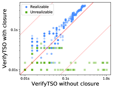
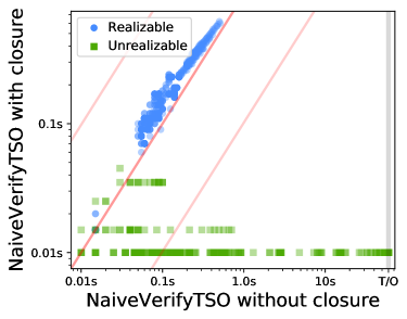
Figure 17. Comparison of $\operatorname{VerifyTSO}$ (left) and $\operatorname{NaiveVerifyTSO}$ (right) with and without closure on verification instances with RMW and CAS instructions.

Finally, Figure 17 presents the effect of closure for $\operatorname{VerifyTSO}$ and $\operatorname{NaiveVerifyTSO}$ on verification instances that contain RMW and CAS instructions. Similarly to the verification without RMW and CAS instructions, both verification algorithms are somewhat slower when using closure on the realizable instances, and they are significantly faster when using closure on the unrealizable instances.

C.3. SMC – Experimental Setup Details

Here we present further details regarding the setup for SMC experiments.

Handling assertion violations. We note that not all benchmarks behave as intended under all memory models, e.g., a benchmark might be correct under $\operatorname{SC}$, but contain bugs under $\operatorname{TSO}$. However, this is not an issue, as our goal is to characterize the size of the underlying partitionings, rather than detecting assertion violations. We have disabled all assertions, in order to not have the measured parameters be affected by how fast a violation is discovered, as the latter is arbitrary. As a sanity check, we have confirmed that for each memory model, all algorithms considered for that model discover the same bugs when assertions are enabled.

Identifying events. Our implementation extends the Nidhugg model checker and we rely on the interpreter built inside Nidhugg to identify events. An event $e$ is defined by a triple ($a_{e},b_{e},c_{e}$), where $a_{e}$ is the thread-id of $e$, $b_{e}$ is the id of either the buffer of $a_{e}$ or the main-thread of $a_{e}$ that $e$ is a part of, and $c_{e}$ is the sequential number of the last LLVM instruction (of the corresponding thread/buffer) that is part of $e$. It can happen that there exist two traces $\sigma_{1}$ and $\sigma_{2}$, and two different events $e_{1}\in\sigma_{1}$, $e_{2}\in\sigma_{2}$, such that their identifiers are equal, i.e., $a_{e_{1}}=a_{e_{2}}$, $b_{e_{2}}=b_{e_{2}}$, and $c_{e_{1}}=c_{e_{2}}$. However, this means that the control-flow leading to each event is different. In this case, $\sigma_{1}$ and $\sigma_{2}$ differ in the reads-from of a common event that is ordered by the program order $\mathsf{PO}$ both before $e_{1}$ in $\sigma_{1}$ and before $e_{2}$ in $\sigma_{2}$, and hence $e_{1}$ and $e_{2}$ are treated as inequivalent.

Dynamic thread creation. For simplicity of presentation of our approach, we have neglected dynamic thread creation and assumed a static set of threads for a given concurrent program. In practice, all our benchmarks spawn threads dynamically. This situation is handled straightforwardly, by including in the program order $\mathsf{PO}$ the orderings naturally induced by spawn and join events.

Benchmark adaptations. We have made small changes to some of the SVCOMP benchmarks so they can be processed by our prototype implementation in Nidhugg:

• Verifier calls to perform acquire and release are handled by a pthread_mutex.

• In order to eliminate intra-thread nondeterminism, verifier calls to nondeterministically produce an arbitrary integer are replaced by a constant value.

Further, we have made steps to obtain scalable versions of benchmarks:

• In mutual exclusion benchmarks, the thread routines are put in a loop with scalable size, so threads can reenter a critical section multiple times.

• We manually perform loop unrolling, i.e., we limit the amount of times each loop is executed by a scalable bound, instead of relying on the loop bounding technique provided by Nidhugg.

C.4. SMC – Full Experimental Results

Here we provide full results of the SMC experiments. We first provide several further scatter plots to compactly illustrate the full experimental results. For each fixed plot comparing two algorithms, we plot the execution times and the numbers of explored maximal traces as follows. For each benchmark, we consider the highest attempted unroll bound where both compared algorithms finish before the one-hour timeout. Then we plot the time and the number of traces obtained by the two algorithms on the benchmark scaled with the above unroll bound.

In each plot, the opaque (resp. semi-transparent) red line represents identity (resp. order-of-magnitude improvement). Green dots indicate that a trace reduction was achieved on the underlying benchmark by the algorithm on the y-axis, as compared to the algorithm on the x-axis. Benchmarks with no trace reduction are represented by blue dots.

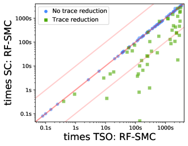
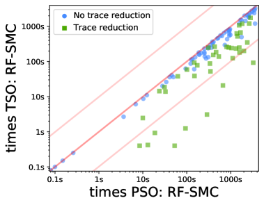
Figure 18. Times comparison as $\operatorname{RF-SMC}$ moves from $\operatorname{SC}$ to $\operatorname{TSO}$ (left) and from $\operatorname{TSO}$ to $\operatorname{PSO}$ (right).

Figure 18 captures how analyzing a concurrent program by $\operatorname{RF-SMC}$ under more relaxed memory settings affects the execution time. Unsurprisingly, when a program exhibits additional behavior under a more relaxed model, more time is required to fully analyze it under the more relaxed model. Green dots represent such programs. On the other hand, for programs (represented by blue dots) where the number of traces stays the same in the more relaxed model, the time required for analysis is only minorly impacted.

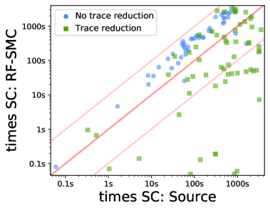
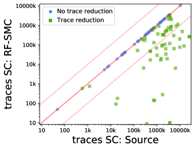
Figure 19. Times (left) and traces (right) comparison for $\operatorname{RF-SMC}$ and $\mathsf{Source}$ on the $\operatorname{SC}$ memory model.

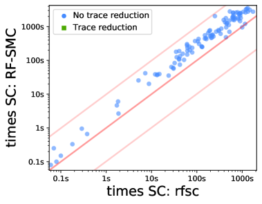
Figure 20. Times comparison for $\operatorname{RF-SMC}$ and $\mathsf{rfsc}$ on the $\operatorname{SC}$ memory model (traces coincide).

Figure 19 compares in $\operatorname{SC}$ the algorithm $\mathsf{Source}$ with our algorithm $\operatorname{RF-SMC}$ that handles $\operatorname{SC}$ as $\operatorname{TSO}$ where a fence event is inserted after every buffer-write event. Similar trends are observed as when $\mathsf{Source}$ and $\operatorname{RF-SMC}$ are compared in $\operatorname{TSO}$ and $\operatorname{PSO}$. Specifically, there are cases where the RF partitioning offers reduction of the trace space size to be explored (green dots), and this often leads to significant speedup of the exploration. On the other hand, $\mathsf{Source}$ dominates in cases where no RF-based partitioning is induced (blue dots).

Further, Figure 20 compares in $\operatorname{SC}$ the algorithm $\operatorname{RF-SMC}$ with $\mathsf{rfsc}$, the reads-from SMC algorithm for $\operatorname{SC}$ presented by Abdulla et al. (2019). These two are essentially identical algorithms, thus unsurprisingly, the number of explored traces coincides in all cases. However, the well-engineered implementation of $\mathsf{rfsc}$ is faster than our implementation of $\operatorname{RF-SMC}$. This comparison provides a rough illustration of the effect of the optimizations and data-structures recently employed by $\mathsf{rfsc}$ in the work of Lång and Sagonas (2020).

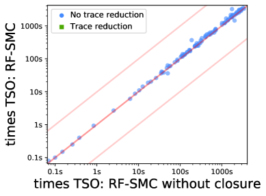
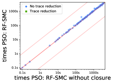
Figure 21. Times comparison for $\operatorname{RF-SMC}$ with and without closure on $\operatorname{TSO}$ (left) and $\operatorname{PSO}$ (right) memory models (traces coincide).

In Section C.2 we have seen that utilizing closure in consistency verification of realizable instances is mostly detrimental, whereas in consistency verification of unrealizable cases it is extremely helpful. This naturally begs a question whether it is overall beneficial to use closure in SMC. The plots in Figure 21 present the results for such an experiment. The plots demonstrate that the time differences are negligible. The number of traces is, unsurprisingly, unaffected (it is also supposed to be unaffected, since closure is sound and $\operatorname{VerifyTSO}$/$\operatorname{VerifyPSO}$ are sound and complete).

We have further considered an auxiliary-trace heuristic for guiding $\operatorname{VerifyTSO}$ resp. $\operatorname{VerifyPSO}$, similar to the heuristic reported by Abdulla et al. (2019). Similar to the paragraph above, this heuristic provided little-to-no time difference in the model checking task in our experiments.

Benchmark		U	Sequential Consistency			Total Store Order		Partial Store Order
			$\mathsf{rfsc}$	$\operatorname{RF-SMC}$	$\mathsf{Source}$	$\operatorname{RF-SMC}$	$\mathsf{Source}$	$\operatorname{RF-SMC}$	$\mathsf{Source}$
approxds_append threads: U	Traces	5	9945	9945	127740	9945	127740	9945	127740
		6	198936	198936	9847080	198936	9847080	198936	9847080
	Times	5	3.00s	9.64s	32s	9.55s	29s	14s	25s
		6	68s	254s	3161s	249s	3068s	368s	2871s
check_bad_array threads: U	Traces	6	75921	75921	357368	75921	357368	75921	357368
		7	1115240	1115240	8245810	1115240	8245810	1115240	-
	Times	6	20s	42s	102s	43s	94s	48s	284s
		7	300s	790s	3524s	802s	2418s	893s	-
circular_buffer threads: 2	Traces	10	184756	184756	184756	184756	184756	184756	184756
		11	705432	705432	705432	705432	705432	-	705432
	Times	10	140s	442s	83s	435s	91s	831s	99s
		11	639s	2140s	431s	2140s	408s	-	383s
control_flow threads: 2U+2	Traces	7	143	143	720720	143	720720	143	720720
		14	16413	16413	-	16413	-	16413	-
	Times	7	0.08s	0.19s	310s	0.19s	273s	0.21s	293s
		14	7.28s	42s	-	41s	-	45s	-
dispatcher threads: U+1	Traces	4	6854	6854	6854	6854	6854	6854	6854
		5	151032	151032	151032	151032	151032	151032	151032
	Times	4	8.16s	16s	22s	17s	23s	23s	22s
		5	334s	612s	901s	625s	1052s	935s	1064s
electron_microscope threads: 2	Traces	3	984	984	984	984	984	90866	90866
		4	20347	20347	20347	20347	20347	-	11613535
	Times	3	0.31s	0.41s	0.12s	0.40s	0.14s	53s	22s
		4	5.58s	9.46s	1.82s	9.06s	3.29s	-	2479s
eratosthenes threads: 2	Traces	13	535	535	3358	1467	32800	3375	175616
		17	4667	4667	100664	29217	4719488	253125	-
	Times	13	0.20s	0.49s	0.69s	1.05s	19s	3.62s	277s
		17	2.12s	6.70s	46s	32s	2978s	475s	-
exponential_bug threads: 3	Traces	20	502771	502771	538332	503714	538332	581482	-
		25	1063451	1063451	1644109	1064879	1644109	1204567	-
	Times	20	172s	505s	91s	490s	87s	770s	-
		25	412s	1236s	297s	1195s	500s	1831s	-
filesystem threads: U	Traces	24	2048	2048	2048	2048	2048	2048	2048
		26	8192	8192	8192	8192	8192	8192	8192
	Times	24	6.99s	13s	6.71s	13s	3.92s	32s	6.16s
		26	30s	60s	29s	61s	17s	148s	20s
floating_read threads: U	Traces	7	8	8	40320	8	40320	8	40320
		8	9	9	362880	9	362880	9	362880
	Times	7	0.05s	0.05s	8.49s	0.05s	12s	0.05s	30s
		8	0.07s	0.05s	81s	0.05s	128s	0.05s	267s
lastwrite threads: U	Traces	9	9	9	362880	9	362880	9	362880
		10	10	10	3628800	10	3628800	10	3628800
	Times	9	0.05s	0.05s	77s	0.05s	61s	0.05s	64s
		10	0.05s	0.05s	846s	0.05s	868s	0.06s	757s
lastzero threads: U+1	Traces	14	69632	69632	69632	69632	69632	69632	69632
		15	147456	147456	147456	147456	147456	147456	147456
	Times	14	20s	121s	425s	119s	532s	127s	308s
		15	53s	308s	1597s	303s	1359s	320s	1143s
account threads: U+1	Traces	4	3125	3125	14400	3125	14400	3125	14400
		5	46656	46656	518400	46656	518400	46656	518400
	Times	4	0.83s	1.57s	2.17s	1.55s	3.33s	1.72s	2.92s
		5	13s	28s	69s	28s	73s	31s	77s
airline threads: U	Traces	5	3125	3125	14400	3125	14400	3125	14400
		6	46656	46656	518400	46656	518400	46656	518400
	Times	5	0.91s	1.87s	3.69s	1.86s	4.05s	2.26s	3.48s
		6	8.82s	34s	92s	34s	122s	41s	157s
bubblesort threads: U	Traces	2	10	10	10	10	10	10	10
		3	51216	51216	143448	51216	143448	57702	143448
	Times	2	0.05s	0.05s	0.05s	0.05s	0.05s	0.05s	0.05s
		3	12s	39s	25s	38s	34s	63s	29s
rv_example threads: 3	Traces	25	102028	102028	180478	102028	180478	107303	180478
		30	169383	169383	295848	169383	295848	176988	295848
	Times	25	50s	124s	61s	125s	53s	157s	61s
		30	131s	250s	108s	248s	126s	311s	132s

Table 2. Part1: Related papers and works, and synthetic benchmarks.

Benchmark		U	Sequential Consistency			Total Store Order		Partial Store Order
			$\mathsf{rfsc}$	$\operatorname{RF-SMC}$	$\mathsf{Source}$	$\operatorname{RF-SMC}$	$\mathsf{Source}$	$\operatorname{RF-SMC}$	$\mathsf{Source}$
multiprodcon threads: 2U	Traces	4	1944	1944	1944	1944	1944	1944	1944
		5	29160	29160	29160	29160	29160	29160	29160
	Times	4	2.13s	4.17s	2.48s	4.26s	1.43s	5.63s	2.28s
		5	32s	84s	42s	87s	31s	123s	34s
opt_lock2 threads: 2	Traces	8	91	91	16714	119	23098	315	194470
		12	139	139	785662	183	1085758	667	-
	Times	8	0.10s	0.09s	3.56s	0.10s	8.33s	0.31s	54s
		12	0.08s	0.13s	137s	0.15s	386s	0.92s	-
opt_lock3 threads: 3	Traces	2	3103	3103	69252	5080	217992	7852	435798
		3	87451	87451	15036174	151570	-	425260	-
	Times	2	0.55s	1.47s	6.75s	2.23s	47s	4.27s	115s
		3	28s	54s	2049s	88s	-	337s	-
overtake threads: U	Traces	3	826	826	6168	826	6168	2197	79092
		4	62893	62893	2418000	62893	2418000	194481	-
	Times	3	0.25s	0.40s	0.82s	0.40s	0.71s	1.37s	33s
		4	15s	39s	605s	39s	482s	150s	-
parker threads: 2	Traces	40	299347	299347	334487	323868	370448	345931	403951
		50	576177	576177	643602	622828	712303	-	777181
	Times	40	285s	989s	223s	1083s	180s	1563s	291s
		50	535s	2807s	338s	3216s	425s	-	703s
pgsql threads: 2	Traces	3	3906	3906	3906	3906	3906	166666	555546
		4	335923	335923	335923	335923	335923	-	-
	Times	3	1.01s	3.21s	0.91s	3.10s	0.56s	289s	127s
		4	109s	432s	90s	422s	70s	-	-
poke threads: U+8	Traces	4	1946	2636	2636	2636	2636	2636	2636
		5	4903	7079	7079	7079	7079	7079	7079
	Times	4	2.98s	7.61s	11s	7.77s	9.57s	9.94s	6.96s
		5	5.16s	26s	58s	26s	50s	34s	34s
ra threads: U	Traces	5	1296	1296	14400	1296	14400	1296	14400
		6	16807	16807	518400	16807	518400	16807	518400
	Times	5	0.39s	0.72s	3.25s	0.73s	5.82s	0.79s	3.34s
		6	4.94s	11s	76s	11s	123s	12s	236s
race_parametric threads: 2	Traces	6	73789	73789	372436	73789	372436	73789	372436
		7	616227	616227	4027216	616227	4027216	616227	4027216
	Times	6	47s	228s	119s	187s	226s	221s	115s
		7	630s	2566s	1559s	2090s	1931s	2388s	1395s
readers threads: U+1	Traces	14	16384	16384	16384	16384	16384	16384	16384
		15	32768	32768	32768	32768	32768	32768	32768
	Times	14	8.00s	28s	7.77s	28s	8.63s	42s	7.26s
		15	27s	64s	15s	63s	18s	95s	16s
redundant_co threads: 2	Traces	5	91	91	16632	91	16632	91	16632
		40	4921	4921	-	4921	-	4921	-
	Times	5	0.06s	0.07s	1.04s	0.07s	2.17s	0.07s	2.49s
		40	1.83s	6.05s	-	6.09s	-	6.89s	-
seqlock threads: U+1	Traces	7	181440	181440	181440	181440	181440	181440	181440
		8	1814400	1814400	1814400	1814400	1814400	-	1814400
	Times	7	112s	235s	77s	239s	88s	307s	88s
		8	1058s	2741s	813s	2862s	967s	-	1089s
seqlock_atomic threads: U+1	Traces	4	29804	29804	29804	29804	29804	29804	29804
		5	605070	605070	605070	605070	605070	605070	605070
	Times	4	12s	26s	9.74s	27s	10s	32s	13s
		5	267s	710s	254s	732s	271s	930s	362s
spammer threads: U	Traces	4	178	178	19448	256	331776	256	331776
		7	569871	569871	-	823543	-	823543	-
	Times	4	0.15s	0.14s	5.14s	0.17s	69s	0.25s	80s
		7	1001s	954s	-	1204s	-	3592s	-
writer_reader threads: 2	Traces	11	705432	705432	705432	705432	705432	705432	705432
		12	2704156	2704156	2704156	2704156	2704156	2704156	2704156
	Times	11	82s	193s	48s	201s	56s	231s	93s
		12	411s	797s	258s	842s	206s	963s	410s

Table 3. Part2: Related papers and works, and synthetic benchmarks.

Benchmark		U	Sequential Consistency			Total Store Order		Partial Store Order
			$\mathsf{rfsc}$	$\operatorname{RF-SMC}$	$\mathsf{Source}$	$\operatorname{RF-SMC}$	$\mathsf{Source}$	$\operatorname{RF-SMC}$	$\mathsf{Source}$
01_inc threads: U	Traces	5	14400	14400	14400	14400	14400	14400	14400
		6	518400	518400	518400	518400	518400	518400	518400
	Times	5	3.08s	8.85s	3.68s	8.93s	3.90s	9.83s	2.02s
		6	150s	443s	101s	451s	100s	494s	96s
02_inc_cas threads: U	Traces	3	432	432	432	432	432	432	432
		4	159552	159552	159552	159552	159552	159552	159552
	Times	3	0.18s	0.22s	0.09s	0.22s	0.09s	0.24s	0.13s
		4	40s	112s	24s	114s	37s	127s	25s
03_incdec threads: U	Traces	5	14568	14568	14568	14568	14568	14568	14568
		6	2289708	2289708	2289708	2289708	2289708	2289708	2289708
	Times	5	3.67s	9.30s	2.74s	9.42s	3.48s	12s	5.11s
		6	866s	2410s	469s	2393s	747s	3434s	662s
13_unverif threads: U	Traces	5	14400	14400	14400	14400	14400	14400	14400
		6	518400	518400	518400	518400	518400	518400	518400
	Times	5	3.20s	9.31s	2.99s	9.47s	2.29s	10s	3.03s
		6	158s	464s	125s	467s	100s	518s	178s
18_read_write_lock threads: U+2	Traces	6	149912	149912	149912	149912	149912	149912	149912
		7	1349280	1349280	1349280	1349280	1349280	1349280	1349280
	Times	6	69s	160s	54s	159s	66s	218s	42s
		7	805s	1819s	603s	1834s	687s	2559s	536s
27_Boop threads: U+1	Traces	2	165	165	364	205	536	713	14604
		3	68083	68083	966834	100897	2157426	447739	-
	Times	2	0.10s	0.10s	0.08s	0.11s	0.10s	0.36s	2.65s
		3	14s	38s	185s	52s	360s	347s	-
27_Boop4 threads: 4	Traces	4	197260	197260	3873348	313336	9412428	1807408	-
		7	2101147	2101147	-	3933691	-	-	-
	Times	4	33s	124s	550s	182s	2556s	1593s	-
		7	437s	1783s	-	3016s	-	-	-
30_Function_Pointer threads: U+1	Traces	5	30240	30240	30240	30240	30240	30240	30240
		6	665280	665280	665280	665280	665280	665280	665280
	Times	5	7.52s	17s	5.74s	18s	7.23s	19s	7.62s
		6	207s	537s	114s	553s	157s	584s	174s
32_pthread5 threads: U+2	Traces	2	1470	1470	1890	1470	1890	1470	1890
		3	226800	226800	302400	226800	302400	226800	302400
	Times	2	0.55s	0.75s	0.50s	0.75s	0.28s	1.00s	0.31s
		3	79s	172s	75s	170s	72s	253s	59s
40_barrier threads: U	Traces	6	2670	2670	2670	2670	2670	2670	2670
		7	18732	18732	18732	18732	18732	18732	18732
	Times	6	1.12s	2.23s	0.82s	2.27s	0.88s	3.09s	0.61s
		7	8.78s	20s	8.52s	20s	6.78s	28s	7.79s
45_monabsex1 threads: U	Traces	6	16807	16807	518400	16807	518400	16807	518400
		7	262144	262144	25401600	262144	-	262144	-
	Times	6	1.93s	9.02s	49s	8.78s	130s	9.50s	129s
		7	35s	180s	3123s	181s	-	188s	-
46_monabsex2 threads: U	Traces	6	16807	16807	518400	16807	518400	16807	518400
		7	262144	262144	25401600	262144	25401600	262144	-
	Times	6	1.97s	9.00s	53s	8.79s	60s	11s	161s
		7	41s	189s	3229s	185s	3245s	251s	-
47_ticket_hc threads: U	Traces	1	1	1	1	1	1	1	1
		2	48	48	48	48	48	48	48
	Times	1	0.05s	0.05s	0.05s	0.05s	0.07s	0.05s	0.07s
		2	0.06s	0.08s	0.06s	0.08s	0.06s	0.08s	0.08s
48_ticket_low threads: U	Traces	3	204	204	204	204	204	204	204
		4	41400	41400	41400	41400	41400	41400	41400
	Times	3	0.09s	0.15s	0.08s	0.15s	0.08s	0.18s	0.08s
		4	13s	37s	8.33s	36s	9.85s	50s	11s
fib_bench threads: 2	Traces	6	73789	73789	73789	226512	226512	226512	226512
		7	616227	616227	616227	2760615	2760615	2760615	2760615
	Times	6	19s	42s	15s	143s	44s	170s	43s
		7	162s	426s	84s	2157s	462s	2561s	489s
fillarray_false threads: 2	Traces	3	14625	14625	47892	14625	59404	14625	63088
		4	471821	471821	2278732	471821	3023380	471821	3329934
	Times	3	5.73s	12s	6.18s	12s	12s	18s	39s
		4	151s	553s	331s	547s	778s	930s	2844s

Table 4. Part1: SVCOMP benchmarks.

Benchmark		U	Sequential Consistency			Total Store Order		Partial Store Order
			$\mathsf{rfsc}$	$\operatorname{RF-SMC}$	$\mathsf{Source}$	$\operatorname{RF-SMC}$	$\mathsf{Source}$	$\operatorname{RF-SMC}$	$\mathsf{Source}$
fillarray_true threads: 2	Traces	2	9	9	10	3334	9820	3334	10076
		3	11	11	12	131636	594054	131636	630894
	Times	2	0.05s	0.05s	0.05s	2.30s	1.86s	3.86s	5.14s
		3	0.05s	0.05s	0.05s	139s	148s	257s	652s
fk2012_1p1c threads: 2	Traces	15	1999336	1999336	3236936	1999336	3236936	1999336	3236936
		16	2399193	2399193	3884313	2399193	3884313	2399193	3884313
	Times	15	1032s	2652s	632s	2474s	2208s	2780s	2437s
		16	1476s	3133s	888s	3059s	3006s	3410s	2792s
fk2012_1p2c threads: 3	Traces	3	33886	33886	42144	33886	42144	33886	42144
		4	888404	888404	1217826	888404	1217826	888404	1217826
	Times	3	15s	19s	5.03s	19s	6.75s	21s	11s
		4	523s	704s	250s	718s	253s	787s	300s
fk2012_2p1c threads: 3	Traces	12	1250886	1250886	1931566	1250886	1931566	1250886	1931566
		13	2059540	2059540	3230710	2059540	3230710	2059540	3230710
	Times	12	913s	1565s	406s	1542s	958s	1712s	1176s
		13	1734s	2770s	905s	2791s	1726s	3004s	1893s
fk2012_2p2c threads: 4	Traces	2	3556	3556	3680	3556	3680	3556	3680
		3	129120	129120	145068	129120	145068	129120	145068
	Times	2	0.96s	2.14s	1.04s	2.16s	0.66s	2.39s	0.63s
		3	52s	104s	29s	104s	50s	114s	34s
fkp2013 threads: U+1	Traces	6	117649	117649	3628800	117649	3628800	117649	3628800
		7	2097152	2097152	-	2097152	-	2097152	-
	Times	6	13s	64s	418s	63s	437s	69s	1200s
		7	391s	1575s	-	1530s	-	1677s	-
fkp2014 threads: U	Traces	3	1098	1098	1098	1098	1098	1098	1098
		4	207024	207024	207024	207024	207024	207024	207024
	Times	3	0.24s	0.54s	0.16s	0.55s	0.22s	1.05s	0.17s
		4	49s	157s	31s	157s	29s	194s	48s
gcd threads: 2	Traces	25	61302	61302	61302	61302	61302	61302	61302
		30	106262	106262	106262	106262	106262	106262	106262
	Times	25	62s	154s	26s	154s	33s	165s	42s
		30	105s	366s	54s	368s	57s	383s	47s
indexer threads: U	Traces	15	4096	4096	4096	4096	4096	4096	4096
		16	32768	32768	32768	32768	32768	32768	32768
	Times	15	18s	53s	16s	51s	16s	181s	15s
		16	197s	520s	114s	499s	131s	1772s	110s
nondet-array threads: U	Traces	6	75486	75486	9854640	75486	9854640	75486	-
		7	1649221	1649221	-	1649221	-	1649221	-
	Times	6	28s	52s	2779s	50s	2532s	70s	-
		7	521s	1512s	-	1445s	-	2163s	-
nondet-loop-variant threads: U+1	Traces	6	5040	5040	5040	5040	5040	5040	5040
		7	40320	40320	40320	40320	40320	40320	40320
	Times	6	2.15s	3.67s	1.18s	3.70s	1.16s	4.18s	1.33s
		7	24s	35s	11s	36s	8.78s	41s	7.09s
pthread-datarace threads: 2	Traces	6	99442	99442	372436	99442	372436	99442	372436
		7	829168	829168	4027216	829168	4027216	829168	4027216
	Times	6	19s	34s	53s	34s	75s	40s	50s
		7	115s	332s	565s	334s	807s	389s	547s
queue_ok threads: U+1	Traces	6	5040	5040	5040	5040	5040	5040	5040
		7	40320	40320	40320	40320	40320	40320	40320
	Times	6	8.29s	30s	4.93s	29s	7.76s	72s	8.08s
		7	61s	303s	52s	296s	62s	736s	50s
qw2004 threads: U+1	Traces	4	28152	28152	28152	28152	28152	28152	-
		5	1354920	1354920	1354920	1354920	1354920	1354920	-
	Times	4	12s	26s	9.15s	26s	5.44s	36s	-
		5	610s	1870s	310s	1893s	353s	2578s	-
reorder_5 threads: U+1	Traces	4	145	145	40032	145	40032	149	54720
		30	54901	54901	-	54901	-	54931	-
	Times	4	0.07s	0.11s	7.66s	0.11s	8.97s	0.13s	25s
		30	61s	278s	-	265s	-	430s	-
scull_Rloop threads: 3	Traces	3	148684	148684	617706	148684	617706	478024	5397158
		4	569409	569409	2732933	569409	2732933	-	-
	Times	3	104s	242s	338s	235s	350s	1324s	2574s
		4	508s	1123s	1152s	1080s	1550s	-	-

Table 5. Part2: SVCOMP benchmarks.

Benchmark		U	Sequential Consistency			Total Store Order		Partial Store Order
			$\mathsf{rfsc}$	$\operatorname{RF-SMC}$	$\mathsf{Source}$	$\operatorname{RF-SMC}$	$\mathsf{Source}$	$\operatorname{RF-SMC}$	$\mathsf{Source}$
scull_Wloop threads: 3	Traces	2	32305	32305	117149	32305	117149	106220	929708
		4	874282	874282	4241286	874282	4241286	-	-
	Times	2	16s	44s	62s	43s	38s	244s	534s
		4	669s	1896s	2130s	1835s	2070s	-	-
scull_loop threads: 3	Traces	1	2491	2491	6992	2491	6992	6188	42636
		2	749811	749811	3157281	749811	3157281	-	-
	Times	1	0.89s	2.52s	2.66s	2.46s	3.13s	9.98s	22s
		2	419s	1354s	1489s	1301s	1499s	-	-
sigma threads: U	Traces	7	30952	30952	135135	30952	135135	30952	135135
		8	325488	325488	2027025	325488	2027025	325488	2027025
	Times	7	7.14s	27s	29s	27s	44s	30s	35s
		8	91s	373s	532s	364s	658s	407s	722s
singleton threads: U+1	Traces	9	9	9	362880	9	362880	9	362880
		10	10	10	3628800	10	3628800	10	-
	Times	9	0.06s	0.06s	142s	0.06s	88s	0.06s	649s
		10	0.08s	0.06s	977s	0.06s	1083s	0.06s	-
sssc12 threads: U	Traces	7	5040	5040	5040	5040	5040	5040	5040
		8	40320	40320	40320	40320	40320	40320	40320
	Times	7	3.46s	11s	4.08s	11s	5.31s	22s	3.31s
		8	36s	124s	49s	122s	35s	275s	36s
sssc12_variant threads: U	Traces	7	5040	5040	5040	5040	5040	5040	5040
		8	40320	40320	40320	40320	40320	40320	40320
	Times	7	4.47s	13s	3.87s	12s	6.89s	24s	8.07s
		8	61s	149s	62s	134s	59s	309s	46s
stack threads: 2	Traces	10	184756	184756	184756	184756	184756	184756	184756
		11	705432	705432	705432	705432	705432	705432	705432
	Times	10	117s	275s	86s	281s	87s	371s	78s
		11	453s	1211s	462s	1216s	357s	1573s	340s

Table 6. Part3: SVCOMP benchmarks.

Benchmark		U	Sequential Consistency			Total Store Order		Partial Store Order
			$\mathsf{rfsc}$	$\operatorname{RF-SMC}$	$\mathsf{Source}$	$\operatorname{RF-SMC}$	$\mathsf{Source}$	$\operatorname{RF-SMC}$	$\mathsf{Source}$
X2Tv1 threads: 2	Traces	4	3851	3851	3851	129946	129946	129946	129946
		5	30737	30737	30737	3976753	3976753	3976753	3976753
	Times	4	1.18s	1.89s	0.94s	64s	24s	75s	36s
		5	10s	18s	8.17s	2581s	812s	3086s	891s
X2Tv10 threads: 2	Traces	2	5079	5079	5079	16282	16282	16282	16282
		3	308433	308433	308433	4225551	4225551	4225551	4225551
	Times	2	0.87s	2.22s	1.11s	7.09s	2.77s	8.13s	4.35s
		3	62s	192s	62s	2915s	1156s	3496s	1047s
X2Tv2 threads: 2	Traces	2	1293	1293	1293	4338	4338	4338	4338
		3	69316	69316	69316	931349	931349	931349	931349
	Times	2	0.36s	0.52s	0.19s	1.68s	1.09s	1.92s	1.16s
		3	16s	36s	9.48s	535s	197s	634s	194s
X2Tv3 threads: 2	Traces	2	1030	1030	1030	2486	2486	2486	2486
		3	33866	33866	33866	290984	290984	290984	290984
	Times	2	0.32s	0.42s	0.19s	0.97s	0.34s	1.12s	0.67s
		3	10s	17s	5.56s	160s	79s	187s	71s
X2Tv4 threads: 2	Traces	3	2907	2907	3164	11210	16127	20804	29165
		4	46275	46275	50340	425612	724832	1292944	2121092
	Times	3	0.82s	1.35s	0.37s	4.77s	2.50s	12s	7.11s
		4	15s	27s	6.65s	242s	172s	1047s	754s
X2Tv5 threads: 2	Traces	3	2985	2985	2985	12145	12145	12145	12145
		4	46161	46161	46161	459543	459543	459543	459543
	Times	3	0.89s	1.35s	0.41s	5.11s	1.72s	6.02s	1.85s
		4	16s	25s	9.83s	257s	112s	307s	103s
X2Tv6 threads: 2	Traces	2	718	718	718	4568	4568	9361	9361
		3	20371	20371	20371	417726	417726	1927527	1927527
	Times	2	0.16s	0.34s	0.12s	1.85s	0.57s	4.74s	1.37s
		3	4.04s	12s	4.77s	249s	74s	1573s	630s

Table 7. Part1: Mutual exclusion benchmarks.

Benchmark		U	Sequential Consistency			Total Store Order		Partial Store Order
			$\mathsf{rfsc}$	$\operatorname{RF-SMC}$	$\mathsf{Source}$	$\operatorname{RF-SMC}$	$\mathsf{Source}$	$\operatorname{RF-SMC}$	$\mathsf{Source}$
X2Tv7 threads: 2	Traces	3	573	573	573	17803	17803	17803	17803
		4	2383	2383	2383	514323	514323	514323	514323
	Times	3	0.14s	0.27s	0.11s	7.68s	2.44s	8.83s	5.29s
		4	0.47s	1.20s	0.36s	296s	86s	348s	130s
X2Tv8 threads: 2	Traces	2	394	394	441	2031	2987	5785	9234
		3	8434	8434	9894	220505	411677	1449109	3012426
	Times	2	0.13s	0.20s	0.09s	0.80s	0.39s	2.83s	1.58s
		3	2.54s	4.65s	1.16s	124s	92s	1112s	806s
X2Tv9 threads: 2	Traces	3	7304	7304	7304	38778	38778	38778	38778
		4	153725	153725	153725	2340172	2340172	2340172	2340172
	Times	3	1.23s	3.21s	0.79s	17s	9.01s	20s	5.16s
		4	29s	87s	29s	1528s	399s	1765s	486s
bakery threads: 2	Traces	1	41	41	41	73	73	77	77
		2	7795	7795	7795	25127	25127	28749	28749
	Times	1	0.06s	0.07s	0.06s	0.08s	0.06s	0.10s	0.07s
		2	2.16s	5.63s	1.72s	19s	11s	31s	13s
bakery3 threads: 3	Traces	1	5296	5296	5296	16315	16315	17588	17588
		2	-	-	-	-	-	-	-
	Times	1	1.72s	4.64s	1.63s	14s	6.33s	24s	7.37s
		2	-	-	-	-	-	-	-
burns threads: 2	Traces	2	342	342	342	2989	2989	2989	2989
		3	6887	6887	6887	213915	213915	213915	213915
	Times	2	0.11s	0.19s	0.16s	1.23s	0.51s	1.38s	0.47s
		3	1.64s	3.74s	2.23s	117s	43s	135s	59s
burns3 threads: 3	Traces	1	849	849	849	23502	23502	23502	23502
		2	1490331	1490331	1490331	-	-	-	-
	Times	1	0.21s	0.44s	0.18s	11s	7.74s	12s	8.83s
		2	458s	1287s	485s	-	-	-	-
dekker threads: 2	Traces	4	28595	28595	28595	29044	29044	53349	83333
		5	435245	435245	435245	441810	441810	947754	1636946
	Times	4	6.18s	13s	3.88s	13s	6.03s	35s	17s
		5	128s	259s	56s	262s	80s	808s	289s
dijkstra threads: 2	Traces	2	319	319	319	540	540	9961	9961
		4	353859	353859	353859	2196640	2196640	-	-
	Times	2	0.15s	0.27s	0.25s	0.42s	0.22s	13s	6.29s
		4	207s	462s	157s	2927s	1234s	-	-
dijkstra3 threads: 3	Traces	1	741	741	1192	1120	1934	12328	19330
		2	-	-	-	-	-	-	-
	Times	1	0.38s	0.66s	0.52s	0.93s	0.78s	19s	36s
		2	-	-	-	-	-	-	-
kessels threads: 2	Traces	2	624	624	624	3779	3779	3779	3779
		3	13856	13856	13856	356844	356844	356844	356844
	Times	2	0.15s	0.27s	0.11s	1.36s	0.84s	1.58s	0.51s
		3	2.96s	6.61s	1.71s	177s	48s	212s	83s
lamport threads: 2	Traces	2	1456	1456	3940	2449	10652	100521	473670
		3	130024	130024	741370	367113	3887642	-	-
	Times	2	0.51s	0.77s	0.86s	1.25s	1.86s	94s	456s
		3	41s	105s	128s	301s	766s	-	-
peterson threads: 2	Traces	3	1609	1609	1686	9251	29546	15925	48500
		4	20161	20161	21120	263916	1359890	744888	3286070
	Times	3	0.27s	0.68s	0.19s	3.55s	6.73s	8.13s	9.87s
		4	3.48s	10s	2.99s	138s	314s	537s	710s
pet_fischer threads: 2	Traces	2	4386	4386	4386	13895	13895	13895	13895
		3	430004	430004	430004	3786571	3786571	3786571	3786571
	Times	2	0.66s	1.74s	0.85s	5.49s	1.70s	6.35s	3.60s
		3	79s	236s	59s	2342s	618s	2707s	719s
szymanski threads: 2	Traces	1	103	103	103	497	497	497	497
		2	1991	1991	1991	284015	284015	284015	284015
	Times	1	0.08s	0.08s	0.05s	0.17s	0.12s	0.19s	0.09s
		2	0.53s	0.80s	0.20s	132s	52s	155s	63s
tsay threads: 2	Traces	1	45	45	45	63	63	63	63
		2	7469	7469	7469	21597	21597	21597	21597
	Times	1	0.06s	0.06s	0.05s	0.06s	0.05s	0.07s	0.08s
		2	1.94s	3.13s	0.87s	8.72s	2.54s	10s	3.52s

Table 8. Part2: Mutual exclusion benchmarks.

Benchmark		U	Sequential Consistency			Total Store Order		Partial Store Order
			$\mathsf{rfsc}$	$\operatorname{RF-SMC}$	$\mathsf{Source}$	$\operatorname{RF-SMC}$	$\mathsf{Source}$	$\operatorname{RF-SMC}$	$\mathsf{Source}$
bin_noconsec_bu3 threads: 3	Traces	6	11875	11875	110446	36288	710000	155648	5467500
		7	59375	59375	773122	217728	7100000	1245184	-
	Times	6	5.15s	9.49s	38s	29s	192s	201s	2276s
		7	41s	56s	207s	201s	2323s	2002s	-
bin_noconsec_td3 threads: 3	Traces	6	5308	5308	50960	29794	661015	69741	3141122
		8	88294	88294	1664672	939466	-	-	-
	Times	6	2.30s	5.62s	17s	33s	398s	124s	2456s
		8	53s	129s	833s	1435s	-	-	-
coin_all_bu3 threads: 3	Traces	3	2673	2673	26624	2673	26624	2673	26624
		4	96294	96294	1704560	98307	1855568	104247	2342912
	Times	3	0.85s	1.18s	4.13s	1.19s	4.62s	1.75s	7.32s
		4	31s	57s	476s	59s	423s	101s	888s
coin_all_bu4 threads: 4	Traces	1	4	4	24	4	24	4	24
		2	6400	6400	264600	6400	264600	6400	264600
	Times	1	0.05s	0.05s	0.08s	0.05s	0.05s	0.05s	0.05s
		2	1.87s	2.66s	44s	2.68s	43s	3.65s	73s
coin_all_td3 threads: 3	Traces	11	1771	1771	94484	10216	1898566	184561	-
		16	37171	37171	-	590116	-	-	-
	Times	11	2.04s	3.06s	50s	21s	1277s	667s	-
		16	46s	107s	-	2073s	-	-	-
coin_all_td4 threads: 4	Traces	4	946	946	234984	946	234984	946	234984
		7	110182	110182	-	321298	-	-	-
	Times	4	0.59s	0.74s	121s	0.76s	78s	0.99s	117s
		7	75s	176s	-	601s	-	-	-
coin_min_bu3 threads: 3	Traces	14	229550	229550	1713984	271319	2930352	322959	6133248
		15	918794	918794	6865920	1146047	-	1399489	-
	Times	14	136s	220s	481s	261s	839s	546s	3501s
		15	444s	951s	2168s	1214s	-	2647s	-
coin_min_bu4 threads: 4	Traces	9	64000	64000	5556600	64000	5556600	64000	5556600
		10	640000	640000	-	640000	-	640000	-
	Times	9	19s	48s	1589s	47s	1328s	78s	2050s
		10	224s	575s	-	575s	-	983s	-
coin_min_td3 threads: 3	Traces	14	86091	86091	500260	252661	3589906	458256	-
		15	326976	326976	1902262	1328496	-	-	-
	Times	14	60s	177s	211s	523s	1897s	1433s	-
		15	379s	754s	887s	3066s	-	-	-
coin_min_td4 threads: 4	Traces	9	16682	16682	1470312	19502	4482536	30736	-
		10	230402	230402	-	332182	-	478292	-
	Times	9	13s	24s	521s	28s	1869s	66s	-
		10	188s	741s	-	627s	-	1372s	-
rod_cut_bu3 threads: 3	Traces	6	60396	60396	183516	143259	518676	259857	1302112
		7	362364	362364	1101084	1289881	4765876	-	-
	Times	6	38s	62s	71s	154s	235s	401s	996s
		7	439s	484s	488s	1858s	2668s	-	-
rod_cut_bu4 threads: 4	Traces	2	2008	2008	33912	2008	33912	2008	33912
		3	106500	106500	2246424	135988	3354504	151720	4080168
	Times	2	0.65s	0.94s	6.95s	0.97s	7.32s	1.26s	12s
		3	42s	75s	618s	94s	985s	148s	1975s
rod_cut_td3 threads: 3	Traces	7	20336	20336	102128	99281	762942	184701	1837610
		8	101001	101001	508646	938731	-	-	-
	Times	7	17s	37s	55s	185s	528s	465s	2271s
		8	128s	248s	324s	2330s	-	-	-
rod_cut_td4 threads: 4	Traces	3	1790	1790	91592	1890	144488	2504	184008
		4	33550	33550	2459640	62748	-	103622	-
	Times	3	1.26s	1.36s	29s	1.49s	46s	2.52s	90s
		4	19s	43s	1003s	78s	-	174s	-
lis_bu3 threads: 3	Traces	7	103260	103260	429632	165105	975040	229965	1862144
		8	325740	325740	1744064	596475	4678656	977685	-
	Times	7	76s	99s	191s	168s	511s	338s	2140s
		8	366s	352s	913s	672s	2782s	1675s	-
lis_bu4 threads: 4	Traces	3	28900	28900	1024002	28900	1024002	28900	1024002
		4	1504200	1504200	-	1863700	-	2059000	-
	Times	3	16s	18s	307s	19s	335s	25s	545s
		4	898s	1451s	-	1755s	-	2831s	-

Table 9. Dynamic programming benchmarks.

Related-work benchmarks and synthetic benchmarks.

In Tables 2 and 3 we present benchmarks collected from previous SMC works, namely Abdulla et al. (2019, 2015); Huang and Huang (2016); Chatterjee et al. (2019). The benchmarks contain several examples originating from industrial code, such as parker and pgsql. Further there are several synthetic benchmarks, such as spammer and overtake.

SVCOMP.

In Tables 4, 5 and 6 we present our results on SVCOMP concurrency benchmarks.

Mutual exclusion benchmarks.

In Tables 7 and 8 we present our results for mutual-exclusion algorithms from the literature. We include the classical solutions, and novel solutions presented by Correia and Ramalhete (2016) (prefixed with X2Tv).

Benchmarks on dynamic programming.

Finally, we present benchmarks that perform parallel dynamic programming tasks, introduced by Chatterjee et al. (2019). Table 9 presents the results.

REFERENCES

- (1)
- Abdulla et al. (2014) Parosh Abdulla, Stavros Aronis, Bengt Jonsson, and Konstantinos Sagonas. 2014. Optimal Dynamic Partial Order Reduction (POPL).
- Abdulla et al. (2015) Parosh Aziz Abdulla, Stavros Aronis, Mohamed Faouzi Atig, Bengt Jonsson, Carl Leonardsson, and Konstantinos Sagonas. 2015. Stateless Model Checking for TSO and PSO. In TACAS.
- Abdulla et al. (2019) Parosh Aziz Abdulla, Mohamed Faouzi Atig, Bengt Jonsson, Magnus Lång, Tuan Phong Ngo, and Konstantinos Sagonas. 2019. Optimal Stateless Model Checking for Reads-from Equivalence under Sequential Consistency. Proc. ACM Program. Lang. 3, OOPSLA, Article 150 (Oct. 2019), 29 pages. https://doi.org/10.1145/3360576
- Abdulla et al. (2018) Parosh Aziz Abdulla, Mohamed Faouzi Atig, Bengt Jonsson, and Tuan Phong Ngo. 2018. Optimal stateless model checking under the release-acquire semantics. Proc. ACM Program. Lang. 2, OOPSLA (2018), 135:1–135:29. https://doi.org/10.1145/3276505
- Adve and Gharachorloo (1996) S. V. Adve and K. Gharachorloo. 1996. Shared memory consistency models: a tutorial. Computer 29, 12 (Dec 1996), 66–76. https://doi.org/10.1109/2.546611
- Albert et al. (2017) Elvira Albert, Puri Arenas, María García de la Banda, Miguel Gómez-Zamalloa, and Peter J. Stuckey. 2017. Context-Sensitive Dynamic Partial Order Reduction. In Computer Aided Verification, Rupak Majumdar and Viktor Kunčak (Eds.). Springer International Publishing, Cham, 526–543.
- Albert et al. (2018) Elvira Albert, Miguel Gómez-Zamalloa, Miguel Isabel, and Albert Rubio. 2018. Constrained Dynamic Partial Order Reduction. In Computer Aided Verification, Hana Chockler and Georg Weissenbacher (Eds.). Springer International Publishing, Cham, 392–410.
- Alglave (2010) Jade Alglave. 2010. A Shared Memory Poetics. Ph.D. Dissertation. Paris Diderot University.
- Alglave et al. (2017) Jade Alglave, Patrick Cousot, and Caterina Urban. 2017. Concurrency with Weak Memory Models (Dagstuhl Seminar 16471). Dagstuhl Reports 6, 11 (2017), 108–128. https://doi.org/10.4230/DagRep.6.11.108
- Aronis et al. (2018) Stavros Aronis, Bengt Jonsson, Magnus Lång, and Konstantinos Sagonas. 2018. Optimal Dynamic Partial Order Reduction with Observers. In Tools and Algorithms for the Construction and Analysis of Systems, Dirk Beyer and Marieke Huisman (Eds.). Springer International Publishing, Cham, 229–248.
- Biswas and Enea (2019) Ranadeep Biswas and Constantin Enea. 2019. On the complexity of checking transactional consistency. Proc. ACM Program. Lang. 3, OOPSLA (2019), 165:1–165:28. https://doi.org/10.1145/3360591
- Bouajjani et al. (2013) Ahmed Bouajjani, Egor Derevenetc, and Roland Meyer. 2013. Checking and Enforcing Robustness against TSO. In Programming Languages and Systems, Matthias Felleisen and Philippa Gardner (Eds.). Springer Berlin Heidelberg, Berlin, Heidelberg, 533–553.
- Bouajjani et al. (2011) Ahmed Bouajjani, Roland Meyer, and Eike Möhlmann. 2011. Deciding Robustness against Total Store Ordering. In Automata, Languages and Programming, Luca Aceto, Monika Henzinger, and Jiří Sgall (Eds.). Springer Berlin Heidelberg, Berlin, Heidelberg, 428–440.
- Cain and Lipasti (2002) Harold W. Cain and Mikko H. Lipasti. 2002. Verifying Sequential Consistency Using Vector Clocks. In Proceedings of the Fourteenth Annual ACM Symposium on Parallel Algorithms and Architectures (Winnipeg, Manitoba, Canada) (SPAA ’02). Association for Computing Machinery, New York, NY, USA, 153–154. https://doi.org/10.1145/564870.564897
- Chalupa et al. (2017) Marek Chalupa, Krishnendu Chatterjee, Andreas Pavlogiannis, Nishant Sinha, and Kapil Vaidya. 2017. Data-centric Dynamic Partial Order Reduction. Proc. ACM Program. Lang. 2, POPL, Article 31 (Dec. 2017), 30 pages. https://doi.org/10.1145/3158119
- Chatterjee et al. (2019) Krishnendu Chatterjee, Andreas Pavlogiannis, and Viktor Toman. 2019. Value-Centric Dynamic Partial Order Reduction. Proc. ACM Program. Lang. 3, OOPSLA, Article 124 (Oct. 2019), 29 pages. https://doi.org/10.1145/3360550
- Chen et al. (2009) Y. Chen, Yi Lv, W. Hu, T. Chen, Haihua Shen, Pengyu Wang, and Hong Pan. 2009. Fast complete memory consistency verification. In 2009 IEEE 15th International Symposium on High Performance Computer Architecture. 381–392.
- Chini and Saivasan (2020) Peter Chini and Prakash Saivasan. 2020. A Framework for Consistency Algorithms. In 40th IARCS Annual Conference on Foundations of Software Technology and Theoretical Computer Science, FSTTCS 2020, December 14-18, 2020, BITS Pilani, K K Birla Goa Campus, Goa, India (Virtual Conference) (LIPIcs, Vol. 182), Nitin Saxena and Sunil Simon (Eds.). Schloss Dagstuhl - Leibniz-Zentrum für Informatik, 42:1–42:17. https://doi.org/10.4230/LIPIcs.FSTTCS.2020.42
- Clarke et al. (1999) E.M. Clarke, O. Grumberg, M. Minea, and D. Peled. 1999. State space reduction using partial order techniques. STTT 2, 3 (1999), 279–287.
- Correia and Ramalhete (2016) Andreia Correia and Pedro Ramalhete. 2016. 2-thread software solutions for the mutual exclusion problem. https://github.com/pramalhe/ConcurrencyFreaks/blob/master/papers/cr2t-2016.pdf.
- Demsky and Lam (2015) Brian Demsky and Patrick Lam. 2015. SATCheck: SAT-directed Stateless Model Checking for SC and TSO (OOPSLA). ACM, New York, NY, USA, 20–36. https://doi.org/10.1145/2814270.2814297
- Flanagan and Godefroid (2005) Cormac Flanagan and Patrice Godefroid. 2005. Dynamic Partial-order Reduction for Model Checking Software. In POPL.
- Furbach et al. (2015) Florian Furbach, Roland Meyer, Klaus Schneider, and Maximilian Senftleben. 2015. Memory-Model-Aware Testing: A Unified Complexity Analysis. ACM Trans. Embed. Comput. Syst. 14, 4, Article 63 (Sept. 2015), 25 pages. https://doi.org/10.1145/2753761
- Gibbons and Korach (1997) Phillip B. Gibbons and Ephraim Korach. 1997. Testing Shared Memories. SIAM J. Comput. 26, 4 (Aug. 1997), 1208–1244. https://doi.org/10.1137/S0097539794279614
- Godefroid (1996) P. Godefroid. 1996. Partial-Order Methods for the Verification of Concurrent Systems: An Approach to the State-Explosion Problem. Springer-Verlag, Secaucus, NJ, USA.
- Godefroid (1997) Patrice Godefroid. 1997. Model Checking for Programming Languages Using VeriSoft. In POPL.
- Godefroid (2005) Patrice Godefroid. 2005. Software Model Checking: The VeriSoft Approach. FMSD 26, 2 (2005), 77–101.
- Herlihy and Wing (1990) Maurice P. Herlihy and Jeannette M. Wing. 1990. Linearizability: A Correctness Condition for Concurrent Objects. ACM Trans. Program. Lang. Syst. 12, 3 (July 1990), 463–492. https://doi.org/10.1145/78969.78972
- Hu et al. (2012) W. Hu, Y. Chen, T. Chen, C. Qian, and L. Li. 2012. Linear Time Memory Consistency Verification. IEEE Trans. Comput. 61, 4 (2012), 502–516.
- Huang (2015) Jeff Huang. 2015. Stateless Model Checking Concurrent Programs with Maximal Causality Reduction. In PLDI.
- Huang and Huang (2016) Shiyou Huang and Jeff Huang. 2016. Maximal Causality Reduction for TSO and PSO. SIGPLAN Not. 51, 10 (Oct. 2016), 447–461. https://doi.org/10.1145/3022671.2984025
- Huang and Huang (2017) Shiyou Huang and Jeff Huang. 2017. Speeding Up Maximal Causality Reduction with Static Dependency Analysis. In 31st European Conference on Object-Oriented Programming, ECOOP 2017, June 19-23, 2017, Barcelona, Spain. 16:1–16:22. https://doi.org/10.4230/LIPIcs.ECOOP.2017.16
- Kahlon et al. (2009) Vineet Kahlon, Chao Wang, and Aarti Gupta. 2009. Monotonic Partial Order Reduction: An Optimal Symbolic Partial Order Reduction Technique. In Proceedings of the 21st International Conference on Computer Aided Verification (Grenoble, France) (CAV ’09). Springer-Verlag, Berlin, Heidelberg, 398–413. https://doi.org/10.1007/978-3-642-02658-4_31
- Kini et al. (2017) Dileep Kini, Umang Mathur, and Mahesh Viswanathan. 2017. Dynamic Race Prediction in Linear Time. In Proceedings of the 38th ACM SIGPLAN Conference on Programming Language Design and Implementation (Barcelona, Spain) (PLDI 2017). ACM, New York, NY, USA, 157–170. https://doi.org/10.1145/3062341.3062374
- Kokologiannakis et al. (2017) Michalis Kokologiannakis, Ori Lahav, Konstantinos Sagonas, and Viktor Vafeiadis. 2017. Effective Stateless Model Checking for C/C++ Concurrency. Proc. ACM Program. Lang. 2, POPL, Article 17 (Dec. 2017), 32 pages. https://doi.org/10.1145/3158105
- Kokologiannakis et al. (2019a) Michalis Kokologiannakis, Azalea Raad, and Viktor Vafeiadis. 2019a. Effective Lock Handling in Stateless Model Checking. Proc. ACM Program. Lang. 3, OOPSLA, Article 173 (Oct. 2019), 26 pages. https://doi.org/10.1145/3360599
- Kokologiannakis et al. (2019b) Michalis Kokologiannakis, Azalea Raad, and Viktor Vafeiadis. 2019b. Model Checking for Weakly Consistent Libraries. In Proceedings of the 40th ACM SIGPLAN Conference on Programming Language Design and Implementation (Phoenix, AZ, USA) (PLDI 2019). ACM, New York, NY, USA, 96–110. https://doi.org/10.1145/3314221.3314609
- Kokologiannakis and Vafeiadis (2020) Michalis Kokologiannakis and Viktor Vafeiadis. 2020. HMC: Model Checking for Hardware Memory Models. In ASPLOS ’20: Architectural Support for Programming Languages and Operating Systems, Lausanne, Switzerland, March 16-20, 2020, James R. Larus, Luis Ceze, and Karin Strauss (Eds.). ACM, 1157–1171. https://doi.org/10.1145/3373376.3378480
- Lahav et al. (2017) Ori Lahav, Viktor Vafeiadis, Jeehoon Kang, Chung-Kil Hur, and Derek Dreyer. 2017. Repairing sequential consistency in C/C++11. In Proceedings of the 38th ACM SIGPLAN Conference on Programming Language Design and Implementation, PLDI 2017, Barcelona, Spain, June 18-23, 2017, Albert Cohen and Martin T. Vechev (Eds.). ACM, 618–632. https://doi.org/10.1145/3062341.3062352
- Lamport (1979) L. Lamport. 1979. How to Make a Multiprocessor Computer That Correctly Executes Multiprocess Programs. IEEE Trans. Comput. 28, 9 (1979), 690–691.
- Lång and Sagonas (2020) Magnus Lång and Konstantinos Sagonas. 2020. Parallel Graph-Based Stateless Model Checking. In Automated Technology for Verification and Analysis - 18th International Symposium, ATVA 2020, Hanoi, Vietnam, October 19-23, 2020, Proceedings (Lecture Notes in Computer Science, Vol. 12302), Dang Van Hung and Oleg Sokolsky (Eds.). Springer, 377–393. https://doi.org/10.1007/978-3-030-59152-6_21
- Madan Musuvathi (2007) Tom Ball Madan Musuvathi, Shaz Qadeer. 2007. CHESS: A systematic testing tool for concurrent software. Technical Report.
- Manovit and Hangal (2006) C. Manovit and S. Hangal. 2006. Completely verifying memory consistency of test program executions. In The Twelfth International Symposium on High-Performance Computer Architecture, 2006. 166–175.
- Mathur et al. (2020) Umang Mathur, Andreas Pavlogiannis, and Mahesh Viswanathan. 2020. The Complexity of Dynamic Data Race Prediction. In Proceedings of the 35th Annual ACM/IEEE Symposium on Logic in Computer Science (Saarbrücken, Germany) (LICS ’20). Association for Computing Machinery, New York, NY, USA, 713–727. https://doi.org/10.1145/3373718.3394783
- Mathur et al. (2021) Umang Mathur, Andreas Pavlogiannis, and Mahesh Viswanathan. 2021. Optimal Prediction of Synchronization-Preserving Races (POPL ’21). To Appear.
- Norris and Demsky (2013) Brian Norris and Brian Demsky. 2013. CDSchecker: checking concurrent data structures written with C/C++ atomics. In OOPSLA, Antony L. Hosking, Patrick Th. Eugster, and Cristina V. Lopes (Eds.). ACM, 131–150. https://doi.org/10.1145/2509136.2509514
- Owens et al. (2009) Scott Owens, Susmit Sarkar, and Peter Sewell. 2009. A Better x86 Memory Model: x86-TSO. In Theorem Proving in Higher Order Logics, Stefan Berghofer, Tobias Nipkow, Christian Urban, and Makarius Wenzel (Eds.). Springer Berlin Heidelberg, Berlin, Heidelberg, 391–407.
- Pavlogiannis (2019) Andreas Pavlogiannis. 2019. Fast, Sound, and Effectively Complete Dynamic Race Prediction. Proc. ACM Program. Lang. 4, POPL, Article 17 (Dec. 2019), 29 pages. https://doi.org/10.1145/3371085
- Peled (1993) Doron Peled. 1993. All from One, One for All: On Model Checking Using Representatives. In CAV.
- Podkopaev et al. (2019) Anton Podkopaev, Ori Lahav, and Viktor Vafeiadis. 2019. Bridging the gap between programming languages and hardware weak memory models. Proc. ACM Program. Lang. 3, POPL (2019), 69:1–69:31. https://doi.org/10.1145/3290382
- Rodríguez et al. (2015) César Rodríguez, Marcelo Sousa, Subodh Sharma, and Daniel Kroening. 2015. Unfolding-based Partial Order Reduction. In CONCUR.
- Roemer et al. (2020) Jake Roemer, Kaan Genç, and Michael D. Bond. 2020. SmartTrack: Efficient Predictive Race Detection. In Proceedings of the 41st ACM SIGPLAN Conference on Programming Language Design and Implementation (London, UK) (PLDI 2020). Association for Computing Machinery, New York, NY, USA, 747–762. https://doi.org/10.1145/3385412.3385993
- Sewell et al. (2010) Peter Sewell, Susmit Sarkar, Scott Owens, Francesco Zappa Nardelli, and Magnus O. Myreen. 2010. X86-TSO: A Rigorous and Usable Programmer’s Model for x86 Multiprocessors. Commun. ACM 53, 7 (July 2010), 89–97. https://doi.org/10.1145/1785414.1785443
- Shasha and Snir (1988) Dennis Shasha and Marc Snir. 1988. Efficient and Correct Execution of Parallel Programs That Share Memory. ACM Trans. Program. Lang. Syst. 10, 2 (April 1988), 282–312. https://doi.org/10.1145/42190.42277
- Smaragdakis et al. (2012) Yannis Smaragdakis, Jacob Evans, Caitlin Sadowski, Jaeheon Yi, and Cormac Flanagan. 2012. Sound Predictive Race Detection in Polynomial Time. In Proceedings of the 39th Annual ACM SIGPLAN-SIGACT Symposium on Principles of Programming Languages (Philadelphia, PA, USA) (POPL ’12). ACM, New York, NY, USA, 387–400. https://doi.org/10.1145/2103656.2103702
- SPARC International (1994) CORPORATE SPARC International, Inc. 1994. The SPARC Architecture Manual (Version 9). Prentice-Hall, Inc., Upper Saddle River, NJ, USA.
- Zennou et al. (2019) Rachid Zennou, Ahmed Bouajjani, Constantin Enea, and Mohammed Erradi. 2019. Gradual Consistency Checking. In Computer Aided Verification - 31st International Conference, CAV 2019, New York City, NY, USA, July 15-18, 2019, Proceedings, Part II (Lecture Notes in Computer Science, Vol. 11562), Isil Dillig and Serdar Tasiran (Eds.). Springer, 267–285. https://doi.org/10.1007/978-3-030-25543-5_16
- Zhang et al. (2015) Naling Zhang, Markus Kusano, and Chao Wang. 2015. Dynamic Partial Order Reduction for Relaxed Memory Models. In PLDI.