Validity and Reliability of the Scale Internet Users’ Information Privacy Concern (IUIPC) [Extended Version]

Abstract

Internet Users’ Information Privacy Concerns (IUIPC-10) is one of the most endorsed privacy concern scales. It is widely used in the evaluation of human factors of PETs and the investigation of the privacy paradox. Even though its predecessor Concern For Information Privacy (CFIP) has been evaluated independently and the instrument itself seen some scrutiny, we are still missing a dedicated confirmation of IUIPC-10, itself. We aim at closing this gap by systematically analyzing IUIPC’s construct validity and reliability. We obtained three mutually independent samples DocumentVersionTRwith sample sizes $N_{\mathsf{A}}=205$, $N_{\mathsf{B}}=379$, and $N_{\mathsf{V}}=433$.DocumentVersionConferencewith a total of $N=1031$ participants. We conducted a confirmatory factor analysis (CFA) on our main sample. Having found weaknesses, we established further factor analyses to assert the dimensionality of IUIPC-10. We proposed a respecified instrument IUIPC-8 with improved psychometric properties. Finally, we validated our findings on a validation sample. While we could confirm the overall three-dimensionality of IUIPC-10, we found that IUIPC-10 consistently failed construct validity and reliability evaluations, calling into question the unidimensionality of its sub-scales Awareness and Control. Our respecified scale IUIPC-8 offers a statistically significantly better model and outperforms IUIPC-10’s construct validity and reliability. The disconfirming evidence on the construct validity raises doubts how well IUIPC-10 measures the latent variable information privacy concern. The sub-par reliability could yield spurious and erratic results as well as attenuate relations with other latent variables, such as behavior. Thereby, the instrument could confound studies of human factors of PETs or the privacy paradox, in general.

1 Introduction

Sound measurement instruments are a key ingredient in the investigation of privacy concerns and their impact on human behavior. They act as a measuring stick for privacy concerns themselves as well as a foundational component for substantive composite models. Thereby, they are a crucial keystone in evaluating human factors of PETs and studying the privacy paradox.

While there has been a diversification of instruments on privacy concern and behaviors [60, 45, 16, 63, 12, 9, 53] also documented in systematic reviews on the privacy paradox [37, 22], Internet users’ information privacy concerns (IUIPC) [45] stands out as a widely adopted scale diligently created in an evolutionary fashion, with a sound theoretical underpinning and with systematic factor analyses.

IUIPC is based on Concerns for information privacy (CFIP) [60], itself a popular scale measuring organizational information privacy concern, which has been validated in independent empirical studies [61, 27]. Both CFIP and IUIPC scales have been endorsed by Preibusch [53] as a sound instrument.

We are interested in IUIPC-10, a 10-item privacy concern scale with the three dimensions Control, Awareness, and Collection, because of its strong pedigree for the use in the investigation of human factors of PETs and of the privacy paradox. While it has seen some scrutiny as part of other studies [58, 50] and questions of its validity have become apparent, there has not yet been a dedicated adequately sized factor analysis to confirm its validity.

We aim at two complementary research questions: (i) First, we investigate to what extent the the validity and reliability of IUIPC-10 can be confirmed, focusing especially on validating its factor structure. (ii) Second, we consider under which circumstances IUIPC-10 can be employed most reliably, considering especially the estimation method used. The latter line of inquiry is motivated by design decisions made by Malhotra et al. [45]DocumentVersionTRon the handling measurement level, distribution characteristics, outliers and choice of estimation method, which are at odds with contemporary recommendations for a sound CFA methodology [35, 8, 20]. Hence, we thereby aim at ruling out possible confounders of our direct replication and at offering empirically grounded recommendations derived from our conceptual replications on how to best use IUIPC.

Our Contributions.

To the best of our knowledge, we established the first dedicated adequately-sized independent confirmatory factor analysis of IUIPC-10. We, thereby, offer the first comprehensive disconfirming evidence on the construct validity and reliability of this scale, with wide implications for studies measuring information privacy concern in their endeavor to evaluate the users attitude to PETs or to study the privacy paradox overall. While we could confirm the overall three-dimensionality of the scale, we found weaknesses in factorial and convergent validity as well as reliability, especially rooted the sub-scales Control and Awareness. Those weaknesses appeared consistently across our independent samples and irrespective of CFA estimators used. We propose a respecified scale IUIPC-8 that consistently offers a statistically significantly better fit, stronger construct validity and reliability. In terms of analysis methodology, we build a bridge between replicating the exact design decisions of Malhotra et al. [45] to factor analyses especially adept on non-normal, ordinal following contemporary recommendations.

2 Background

We first introduce the role of privacy concern scales and IUIPC in the research of PETs and the privacy paradox, give an overview of the genesis of IUIPC and discuss earlier analyses vis-à-vis of the contributions of this study in Section 2.1. Second, we consider requirements for sound measurement instruments in Section 2.2. Finally, we explain factor analysis as tool to establish a scale’s construct validity in Section C.1.

2.1 Information Privacy Concern

In defining information privacy concern we focus on the conceptual framework of IUIPC. Malhotra et al. [45, p. 337] refer to Westin’s definition of information privacy as a foundation of their understanding of privacy concern: “the claim of individuals, groups, or institutions to determine for them selves when, how, and to what extent information about them is communicated to others.” Information privacy concern is then defined as “an individual’s subjective views of fairness within the context of information privacy.”

This framing of information privacy concern is well aligned with the interdisciplinary review of privacy studies by Smith et al. [59], which considered privacy concern as the central antecedent of related behavior in their privacy macro model. Of course, the causal impact of privacy concern on behavior has been under considerable scrutiny with the observation of the privacy attitude-behavior dichotomy—the privacy paradox [22]. The intense inquiry of the privacy community into the paradox calls for measuring information privacy concern accurately and reliably. This conviction is rooted in the fact that measurement errors could confound the assessment of users’ privacy concerns and, thereby, alternative explanation for the privacy paradox: If one has not actually measured privacy concern, it can hardly be expected to align with exhibited behavior.

There has been a proliferation of related and distinct instruments for measuring information privacy concernDocumentVersionTR [60, 45, 16, 63, 12, 9]. As a comprehensive comparison would be beyond the scope of this study, we refer to Preibusch’s excellent guide to measuring privacy concern [53] for an overview of the field and shall focus on specific comparisons to IUIPC itself. First, we mention Concern for information privacy (CFIP) [60] a major influence on IUIPC. It consists of four dimensions—Collection, Unauthorized Secondary Use, Improper Access and Errors. While both questionnaires share questions, CFIP focuses on individuals’ concerns about organizational privacy practices and the organization’s responsibilities, IUIPC shifts this focus to Internet users framed as consumers and their perception of fairness and justice in the context of information privacy and online companies.

Internet Privacy Concerns (IPC) [16] considered internet privacy concerns with antecedents of perceived vulnerability and control, antecedents familiar from the Protection Motivation Theory (PMT). In terms of the core scale of privacy concern, Dinev and Hart identified two factors (i) Abuse (concern about misuse of information submitted on the Internet) and (ii) Finding (concern about being observed and specific private information being found out). IPC differs from IUIPC in its focus on misuse rather than just collection of information and of concerns of surveillance.

Buchanan et al.’s Online Privacy Concern and Protection for Use on the Internet (OPC) [12] measure considered three sub-scales—General Caution, Technical Protection (both on behaviors), and Privacy Attitude. Compared to IUIPC, OPC sports a strong focus on item stems eliciting being concerned and on measures through a range of concrete privacy risks. The authors considered concurrent validity with IUIPC, observing a correlation of $r=.246$ between OPC’s privacy concern and the total IUIPC score.

CFIP, IPC and OPC have in common that—unlike IUIPC—they do not explicitly mention the loaded word “privacy.” DocumentVersionTRThis is even more so a distinctive feature of the Indirect Content Privacy (ICP) survey developed by Braunstein et al. [9]. Compared to IUIPC it focuses more on sharing specific kinds of sensitive information, carefully avoiding to mention “privacy” or other loaded words. ICP does not offer a dedicated factor analysis confirming its construct validity and reliability.

2.1.1 Genesis of IUIPC

The scale Internet users’ information privacy concern (IUIPC) was developed by Malhotra et al. [45], by predominately adapting questions of the earlier 15-item scale Concern for information privacy (CFIP) by Smith et al. [60] and by framing the questionnaire for Internet users.

CFIP received independent empirical confirmations of its factor structure, first by Stewart and Segars [61], but also by Harborth and Pape [27] on its German translation. DocumentVersionTRIn a somewhat related yet largely unnoticed analysis of general privacy concern, Castañda et al. [13] considered the factor structure on collection and use sub-factors, bearing distinct similarity to the first two dimensions of CFIP.

Malhotra et al. [45, pp. 338] conceived IUIPC-10 as a second-order reflective scale of information privacy concern, with the dimensions Control, Awareness, and Collection. The authors considered the “act of collection, whether it is legal or illegal,” as the starting point of information privacy concerns. The sub-scale control is founded on the conviction that “individuals view procedures as fair when they are vested with control of the procedures.” Finally, they considered being “informed about data collection and other issues” as central concept to the sub-scale awareness. The authors developed IUIPC in exploratory and confirmatory factor analysis, which we shall review systematically in Section 4.

2.1.2 The Role of Privacy Concern Scales in the Investigation of PETs

The role of privacy concern scales in the investigation of the privacy paradox was well documented in the Systematic Literature Review by Gerber et al. [22]: More than a dozen studies used privacy concern as variable. For instance, Schwaig et al. [56] used IUIPC as instrument in their privacy paradox study.

On human factors of PETs, we have the, e.g., technology acceptance of Tor/JonDonym [30] and anonymous credentials [5]. While these two studies used “perceived anonymity” as a three-item scale, subsequent work by Harborth and Pape used IUIPC as privacy concern scale to evaluate JonDonym[28] and Tor [29].

Furthermore, IUIPC has not only been used in the narrow sense of evaluating the privacy paradox or PETs. Let us highlight a few examples in PoPETS: Pu and Grossklags [54] used a scale adopted from IUIPC Collection (or one of its predecessors) to measure own and friends’ privacy concern in their study social app users’ valuation of interdependent privacy. Gerber et al. [23] used IUIPC to contextualize their investigation on privacy risk perception. Barbosa et al. [4] used IUIPC as main privacy measure to predict changes in smart home device use.

Given that Smith et al.’s privacy macro model [59] centered on privacy concern as antecedent of behavior and that Preibusch [53] recommended IUIPC as a “safe bet,” it is not surprising that IUIPC is high on the list of instruments to analyze privacy paradox or PETs. Thereby, we would expect prolific use of IUIPC in future privacy research and perceive a strong need to substantiate the evidence of its construct validity and reliability.

2.2 Validity and Reliability

When evaluating privacy concern instruments, the dual key questions for privacy researchers interested in the investigation of the human factors of PETs and the privacy paradox are: (i) Are we measuring the hidden latent construct “privacy concern” accurately? (validity) (ii) Are we measuring privacy concern consistently and with an adequate signal-to-noise ratio? (reliability)

Validity refers to whether an instrument measures what it purports to measure. Messick offered an early well-regarded definition of validity as the “integrated evaluative judgment of the degree to which empirical evidence and theoretical rationales support the adequacy and appropriateness of inferences and actions based on test scores” [49]. Validity is inferred—judged in degrees—not measured. DocumentVersionTRThis classic authoritative definition is at odds with a newer ontological approach proposed by Borsboom et al. [7] stating that “a test is valid for measuring an attribute if (a) the attribute exists and (b) variations in the attribute causally produce variation in the measurement outcomes.” In our work, we take a pragmatic empiricist’s approach focusing on the validation procedure and evidence.

2.2.1 Content Validity

Content validity refers to the relevance and representativeness of the content of the instrument, typically assessed by expert judgment. We shall evaluate content validity together in keeping with evidence on the craft of the questionnaire design, incl. question format, language used, question order, and, hence, assess psychometric barriers in the form of biases rooted in the questionnaire wording [52, p. 128].

Priming

PrimingDocumentVersionTR [41] means that mentioning a concept activates it in respondents minds and makes it more easily accessible in subsequent questions. Priming is, for instance, created by the use of a loaded wordDocumentVersionTR [52, pp. 137] such as “security.” It can invoke the respondents’ social desirability bias DocumentVersionTR [42].

Leading questions

Leading questions elicit agreement or specific instances of a general term, introduce a bias towards that lead.DocumentVersionTR [52, pp. 137]

Double-barreled questions

Double-barreled questionsDocumentVersionTR [52, p. 128] consist of two or more questions or clauses, making it difficult for the respondent to decide what to answer to, causing nondifferentiated responses.

Positively-oriented questions

Exclusively using positively framed wording for questions leads to nondifferentiation/straightliningDocumentVersionTR [40] and, thereby, to accommodating the acquiescent response biasDocumentVersionTR [39].

2.2.2 Construct Validity

While Messick [48] considers construct validity [15]Check out how Cook and Campbell 1979 defines construct validity, cf. CFIP p. 182/17, the interpretive meaningfulness, the extent to which an instrument accurately represents a construct, as foremost evaluation of validity, there is a range of confirmatory and disconfirmatory evaluations of validity, often referred to as kinds of validity, even if they only constitute a lens on a whole. For the purposes of this paper, we summarize the terms we will use in our own investigation. DocumentVersionConferenceAppendix C.1 details used factor-analysis concepts.

First, we seek evidence of factorial validity, that is, evidence that that factor composition and dimensionality are sound. While IUIPC is a multidimensional scale with three correlated designated dimensions, we require unidimensionality of each sub-scale, a requirement discussed at length by Gerbing and Anderson [24]. Unidimensional measurement models for sub-scales often correspond to expecting congeneric measures, that is, the scores on an item are the expression of a true score weighted by the item’s loading plus some measurement error, where in the congeneric case neither the loadings nor error variances across items are required to be equal. This property entails that the items of each sub-scale must be conceptually homogeneous. The empirical evidence for factorial validity is the found in the adequacy of the hypothesized model’s fit and passing the corresponding fit hypotheses of a confirmatory factor analysis for the designated factor structure [3, 24, 36]. Specifically, we prioritize the following fit metrics and hypotheses, refering the interested reader to Appendix C.3 for further explanations:

Goodness-of-fit $\chi^{2}$:

Measures the exact fit of a model and gives rise to the accept-support exact-fit test against null hypothesis $H_{\chi^{2},0}$.

RMSEA:

Root Mean Square Estimate of Approximation, an absolute badness-of-fit measure estimated as $\hat{\varepsilon}$ with its $90\%$ confidence interval, yielding a range of fit-tests: close fit, not-close fit, and poor fit with decreasing tightness requirements.

DocumentVersionConferenceFurther common criteria, such as CFI or SRMR, are defined in Appendix C.3.

Convergent validity [26, pp. 675] (convergent coherence) on an item-construct level means that items belonging together, that is, to the same construct, should be observed as related to each other. Similarly, discriminant validity [26, pp. 676] (discriminant distinctiveness) means that items not belonging together, that is, not belonging to the same construct, should be observed as not related to each other. Similarly, on a sub-scale level, we expect factors of the same higher-order construct to relate to each other and, on hierarchical factor level, we expect all 1^st-order factors to load strongly on the 2^nd-order factor.

While a poor local fit and tell-tale residual patterns yield disconfirming evidence for convergent and discriminant validity, further evidence is found evidence inter-item correlation matrices. We expect items belonging to the same sub-scale to be highly correlated (converge on the same construct). At the same time correlation to items of other sub-scales should be low, especially lower than the in-construct correlations [36, pp. 196].

These judgments are substantiated with empirical criteria, where we highlight the following metrics:

Standardized Factor Loadings $\beta$:

$Z$-transformed factor scores, typically reported in factor analysis.

Variance Extracted $R^{2}$:

The factor variance accounted for, giving rise to the Average Variance Extracted ($\mathit{AVE}$) defined subsequently in reliability Section 2.2.3.

Heterotrait-Monotrait Ratio (HTMT)

The Heterotrait-Monotrait Ratio is the ratio of the the avg. correlations of indicators across constructs measuring different phenomena to the avg. correlations of indicators within the same construct [31].

We gain empirical evidence in favor of convergent validity [26, pp. 675] (i) if the variance extracted by an item $R^{2}>.50$ entailing that the standardized factor loading are significant and $\beta>.70$, and (ii) if the internal consistency (defined in Section 2.2.3) is sufficient ($\mathit{AVE}>.50$, $\omega>\mathit{AVE}$, and $\omega>.70$). The analysis yields empirical evidence of discriminant validity [26, pp. 676] (i) if the square root of $\mathit{AVE}$ of a latent variable is greater than the max correlation with any other latent variable (Fornell-Larcker criterion [21]), (ii) if the Heterotrait-Monotrait Ratio (HTMT) is less than $.85$ [31, 1]DocumentVersionTR[31, 1].

2.2.3 Reliability

Reliability is the extent to which a variable is consistent in what is being measured [26, p. 123]. It can further be understood as the capacity of “separating signal from noise” [55, p. 709], quantified by the ratio of true score to observed score variance. [36, pp. 90] We evaluate internal consistency as a means to estimate reliability from a single test application. Internal consistency entails that items that purport to measure the same construct produce similar scores [36, p. 91]. DocumentVersionTRWe note that the validity of indices, such as Cronbach’s $\alpha$, is contingent on the scale being congeneric. We will use the following internal consistency measures:

Cronbach’s $\alpha$:

Is based on the average inter-item correlations. DocumentVersionTRWe report it as comparison to IUIPC, even though it is limited to assess internal consistency reliably only if a scale is truly unidimensionalDocumentVersionTR [55, pp. 733][36, p. 91]. DocumentVersionTR

Guttman’s $\lambda_{6}$:

Measures internal consistency with squared multiple correlations of a set of items.

Congeneric Reliability $\omega$:

The amount of general factor saturation (also called composite reliability [36, pp. 313] or construct reliability (CR) [26, p. 676] depending on the source).

AVE:

Average Variance Extracted (AVE) [36, pp. 313] is the average of the squared standardized loadings of indicators belonging to the same factor.

Thresholds for reliability estimates like Cronbach’s $\alpha$ or Composite Reliability $\omega$ are debated in the field, where many recommendations are based on Nunnally’s original treatment of the subject, but equally often misstated [38]. The often quoted $\alpha\geq.70$ was described by Nunnally only to “save time and energy,” whereas a greater threshold of $.80$ was endorsed for basic research [38]. While that would be beneficial for privacy research as well, we shall adopt reliability metrics $\alpha,\omega\geq.70$ as suggested by Hair et al. [26, p. 676]. We further require $\mathit{AVE}>.50$.

2.3 Factor Analysis as Validation Tool

Factor analysis is an excellent tool to establish construct validity and reliability of an instrument. We introduce factor analysis concepts in the Appendix and assume knowledge of the standard factor analysis with Maximum Likelihood estimation. Here we shall only mention properties of estimators MLM and robust WLS, developed to handle non-normal, ordinal data.

DocumentVersionTR

Alternative Estimators

A maximum-likelihood estimation with robust standard errors and Satorra-Bentler scaled test statistic (MLM) is robust against some deviations from normality [35, p. 122]. Lei and Wu [43, p. 172] submit that Likert items with more than five points approximate continuous measurement enough to use MLM, this stance is not universally endorsed DocumentVersionConference[20, 8]DocumentVersionTR[20, 8, 44].

Kline recommends to use of estimators specializing on ordinal data [35, p. 122], such as robust weighted least squares (WLSMVS). The following explanation summarizes Kline [36, pp. 324]. in general, robust WLS methods associate each indicator with a latent response variable for which the method estimates thresholds that relate the ordinal responses on the indicator to a continuous distribution on the indicator’s latent response variable. Then, the measurement model is evaluated with the latent response variables as indicators, while optimizing to approximate the observed polychoric correlations between the original indicator variables. In addition, the method will compute robust standard errors and corrected test statistics. Because the method also needs to estimate the thresholds, the number of free parameters will be greater than in a comparable ML estimation. Reported estimates and $R^{2}$ relate to the latent response variable, not the original indicators themselves.

Because of the level of indirection and the estimation of non-linearly related thresholds, robust WLS is a quite different kettle of fish than Maximum Likelihood estimation on assumedly continuous variables: they are not easily compared by trivially examining blunt fit indices. The estimates of robust WLS need to be interpreted differently than in ML: they are probit of individuals’ response to an indicator instead of a linear change in an indicator [8]. The thresholds show what factor score is necessary for the respective option of an indicator or higher to be selected with $50\%$ probability.

The advantages and disadvantages of robust WLS have been carefully evaluated in simulation studies with known ground truthDocumentVersionConference [17, 44]DocumentVersionTR [17, 20, 44]: (i) Robust WLS models show little bias in the parameter estimation even es the level of skewness and kurtosis increased. Unlike ML models, do not suffer from out-of-bounds estimations of indicator variables. (ii) There is contradictory evidence on standard errors, where robust WLS may be subject to greater amounts of bias. (iii) $\chi^{2}$fit indices of robust WLS are inflated for larger models or smaller samples. (iv) Robust WLS may inflate correlation estimates.

DocumentVersionTR

2.4 Factor Analysis

Factor analysis is a powerful tool for evaluating the construct validity and reliability of privacy concern instruments. Factor analysis refers to a set of statistical methods that are meant to determine the number and nature of latent variables (LVs) or factors that account for the variation and covariation among a set of observed measures commonly referred to as indicatorsDocumentVersionTR [10].

In general, we distinguish exploratory factor analysis (EFA) and confirmatory factor analysis (CFA), both of which are used to establish and evaluate psychometric instruments, respectively. They are both based on the common factor model, which holds that each indicator variable contributes to the variance of one or more common factors and one unique factor. Thereby, common variance (communality) of related observed measures is attributed to the corresponding latent factor, and unique variance (uniqueness) seen either as variance associated with the indicator or as error variance. DocumentVersionTRWhile in EFA the association of indicators to factors is unconstrained, in CFA this association is governed by a specified measurement model. IUIPC is based on a reflective measurement, that is, the observed measure of an indicator variable is seen as caused by some latent factor. Indicators are thereby endogenous variables, latent variables exogenous variables. Reflective measurement requires that all items of the sub-scale are interchangeable [36, pp. 196]DocumentVersionTR and is closely related to the congeneric measure introduced above.

In this paper, we are largely concerned with covariance-based confirmatory factor analysis (CB-CFA). Therein, the statistical tools aim at estimating coefficients for parameters of the measurement model that best fit the covariance matrix of the observed data. The difference between an observed covariance of the sample and an implied covariance of the model is called a residual.

DocumentVersionTR

2.4.1 Estimators and their Assumptions

DocumentVersionConference

2.5 Estimators and their Assumptions

The purpose of a factor analysis is to estimate free parameters of the model (such as loadings or error variance), which is facilitated by estimators. The choice of estimator matters, because each comes with different strengths and weaknesses, requirements and assumptions that need to be fulfilled for the validity of their use. RedundantContentWhile practitioners sometimes endorse estimators as robust in face of violations, there is an ongoing debate what uses are appropriate or ill-advised. DocumentVersionTR

ML Assumptions

The most commonly used method for confirmatory factor analysis is maximum likelihood (ML) estimation. Among other assumptions, this estimator requires according to Kline [36, pp. 71]: (i) a continuous measurement level, (ii) multi-variate normal distribution(entailing the absence of extreme skewness) [36, pp. 74], and (iii) treatment of influential cases and outliers. The distribution requirements are placed on the endogenous variables: the indicators.

DocumentVersionTR

Violations of Assumptions

These requirements are not always fulfilled in samples researchers are interested in. For instance, a common case at odds with ML-based CFA is the use of Likert items as indicator variables. Likert items are ordinal [26, p. 11] in nature, that is, ordered categories in which the distance between categories is not constant; they thereby require special treatment [36, pp. 323].

Lei and Wu [43] held based on a number of empirical studies that the fit indices of approximately normal ordinal variables with at least five categories are not greatly misleading. However, when ordinal and non-normal is treated as continuous and normal, the fit is underestimated and there is a more pronounced negative bias in estimates and standard errors. While Bovaird and Kozoil [8] acknowledge robustness of the ML estimator with normally distributed ordinal data, they stress that increasingly skewed and kurtotic ordinal data inflate the Type I error rate. In the same vein, Kline [35, p. 122] holds the normality assumption for endogenous variables—the indicators—to be critical.

DocumentVersionTR

Alternative Estimators

A maximum-likelihood estimation with robust standard errors and Satorra-Bentler scaled test statistic (MLM) is robust against some deviations from normality [35, p. 122]. Lei and Wu [43, p. 172] submit that Likert items with more than five points approximate continuous measurement enough to use MLM, this stance is not universally endorsed DocumentVersionConference[20, 8]DocumentVersionTR[20, 8, 44].

Kline recommends to use of estimators specializing on ordinal data [35, p. 122], such as robust weighted least squares (WLSMVS). The following explanation summarizes Kline [36, pp. 324]. in general, robust WLS methods associate each indicator with a latent response variable for which the method estimates thresholds that relate the ordinal responses on the indicator to a continuous distribution on the indicator’s latent response variable. Then, the measurement model is evaluated with the latent response variables as indicators, while optimizing to approximate the observed polychoric correlations between the original indicator variables. In addition, the method will compute robust standard errors and corrected test statistics. Because the method also needs to estimate the thresholds, the number of free parameters will be greater than in a comparable ML estimation. Reported estimates and $R^{2}$ relate to the latent response variable, not the original indicators themselves.

Because of the level of indirection and the estimation of non-linearly related thresholds, robust WLS is a quite different kettle of fish than Maximum Likelihood estimation on assumedly continuous variables: they are not easily compared by trivially examining blunt fit indices. The estimates of robust WLS need to be interpreted differently than in ML: they are probit of individuals’ response to an indicator instead of a linear change in an indicator [8]. The thresholds show what factor score is necessary for the respective option of an indicator or higher to be selected with $50\%$ probability.

The advantages and disadvantages of robust WLS have been carefully evaluated in simulation studies with known ground truthDocumentVersionConference [17, 44]DocumentVersionTR [17, 20, 44]: (i) Robust WLS models show little bias in the parameter estimation even es the level of skewness and kurtosis increased. Unlike ML models, do not suffer from out-of-bounds estimations of indicator variables. (ii) There is contradictory evidence on standard errors, where robust WLS may be subject to greater amounts of bias. (iii) $\chi^{2}$fit indices of robust WLS are inflated for larger models or smaller samples. (iv) Robust WLS may inflate correlation estimates.

DocumentVersionTR

2.5.1 Global and Local Fit

DocumentVersionConference

2.6 Global and Local Fit

The closeness of fit of a factor model to an observed sample is evaluated globally with fit indices as well as locally by inspecting the residuals. We shall focus on the ones Kline [36, p. 269] required as minimal reporting. DocumentVersionTR

Fit Indices

$\chi^{2}(\mathit{df})$:

The $\chi^{2}$ for given degrees of freedom is the likelihood ratio chi-square, as a measure of exact fit.

CFI:

The Bentler Comparative Fit Index is an incremental fit index based on the non-centrality measure comparing selected against the null model.

RMSEA:

Root Mean Square Estimate of Approximation ($\hat{\varepsilon}$) is an absolute index of bad fit, reported with its 90% Confidence Interval $[\hat{\varepsilon}_{\mathsf{UL}},\hat{\varepsilon}_{\mathsf{LL}}]$.

SRMR:

Standardized Root Mean Square Residual is a standardized version of the mean absolute covariance residual, where zero indicates excellent fit.

We mention the Goodness-of-Fit index (GFI) reported by IUIPC, which approximates the proportion of variance explained in relation to the estimated population covariance. It is not recommended as it is substantially impacted by sample size and number of indicatorsDocumentVersionTR [33, 57].

Malhotra et al. [45] adopted a combination rule referring to Hu and BentlerDocumentVersionTR [32], which we will report as HBR, staying comparable with their analysis: “A model is considered to be satisfactory if (i) $\mathsf{CFI}>.95$, (ii) $\mathsf{GFI}>.90$, and (iii) $\mathsf{RMSEA}<.06$.” DocumentVersionTRKline [36] spoke against the reliability of such combination rules.

DocumentVersionTR

Model Comparison

Nested models [36, p. 280], that is, models with can be derived from each other by restricting free parameters, can be well-compared with a Likelihood Ratio $\chi^{2}$ Difference Test (LRT) [36, p. 270]. However, the models we are interested in are non-nested [36, p. 287], because they differ in their observed variables. On ML-estimations, we have the Vuong Likelihood Ratio Test [62] at our disposal to establish statistical inferences on such models.

In addition, we introduce the AIC/BIC family of metrics with formulas proposed by Kline [36, p. 287]:

$$\mathsf{AIC}:=\chi^{2}+2q\qquad\qquad\mathsf{BIC}:=\chi^{2}+q\ln(N),$$

where $q$ is the number of free parameters and $N$ the sample size. We compute CAIC as the even-weighted mean between AIC and BIC. These criteria can be used to compare different models estimated on the same samples, on the same variables, but theoretically also on different subsets of variables. Smaller is better.

Statistical Inference

The $\chi^{2}$ and RMSEA indices offer us statistical inferences of global fit. Such tests can either be accept-support, that is, accepting the null hypothesis supports the selected model, or reject-support, that is, rejecting the null hypothesis supports the selected model. We present them in the order of decreasing demand for close approximation.

Exact Fit:

An accept-support test, in which rejecting the null hypothesis on the model $\chi^{2}$ test implies the model is not an exact approximation of the data. The test is sensitive to the sample size and may reject well-fitting models at greater $N$.

$H_{\chi^{2},0}$:

The model is an exact fit in terms of residuals of the covariance structure.

$H_{\chi^{2},1}$:

The residuals of the model are considered too large for an exact fit.

Close Fit:

An accept-support test, evaluated on the RMSEA $\hat{\varepsilon}$ with zero as best result indicating approximate fit.

$H_{\hat{\varepsilon}\leq.05,0}$:

The model has an approximate fit with RMSEA being less or equal $.05$, $\hat{\varepsilon}\leq.05$.

$H_{\hat{\varepsilon}\leq.05,1}$:

The model does not evidence a close fit.

Not-close Fit:

A reject-support hypothesis operating on the upper limit if the RMSEA 90% CI, $\hat{\varepsilon}_{\mathsf{UL}}$, a significant $p$-value rejecting the not-close fit.

$H_{\hat{\varepsilon}\geq.05,0}$:

The model is not a close fit, $\hat{\varepsilon}_{\mathsf{UL}}\geq.05$.

$H_{\hat{\varepsilon}\geq.05,1}$:

Model approximate fit, $\hat{\varepsilon}_{\mathsf{UL}}<.05$.

Poor Fit:

A reject-support test on the upper limit if the RMSEA 90% CI, $\hat{\varepsilon}_{\mathsf{UL}}$ checking for a poor fit.

$H_{\hat{\varepsilon}\geq.10,0}$:

The model is a poor fit with $\hat{\varepsilon}_{\mathsf{UL}}\geq.10$.

$H_{\hat{\varepsilon}\geq.10,1}$:

Model not a poor fit, $\hat{\varepsilon}_{\mathsf{UL}}<.10$.

DocumentVersionTRWe note that the results for these different hypotheses will not necessarily be consistent. Hence, researchers are encouraged to consider the point estimate $\hat{\varepsilon}$ and its entire 90% confidence interval $[\hat{\varepsilon_{\mathsf{LL}}},\hat{\varepsilon_{\mathsf{UL}}}]$. We recommend to interested readers Kline’s excellent summary of these RMSEA fit tests [36, Topic Box 12.1].

DocumentVersionTR

Local Fit

Even with excellent global fit indices, the inspection of the local fit—evidenced by the residuals—must not be neglected. In fact, Kline [36, p. 269] drives home “Any report of the results without information about the residuals is incomplete.” DocumentVersionTRFor that reason, we also stress the importance of evaluating the local fit, which we will do on correlation and (standardized) covariance residuals. Simply put, a large absolute residual indicates covariation that the model does not approximate well and that may thereby lead to spurious results.

3 Related Work

DocumentVersionTRWhile IUIPC-10 has been one of the most-adopted privacy concern scales in the field, its independent confirmation was limited to analyses in the context of other research questions.

Sipior et al. [58] observed that IUIPC was under-studied at the time, offered a considerate review of the related literature, and focused their lens on the role of trusting and risk beliefs in IUIPC’s causal model. With the caveat of being executed on a small sample of $N=63$ students, their research could “not confirm the use of the IUIPC construct to measure information privacy concerns.” Even though they also excluded one control item, their concerns, however, were mostly focused on the causal structure of IUIPC and not on the soundness of the underlying measurement model of IUIPC-10. Our study goes beyond Sipior et al.’s by evaluating the heart of IUIPC, that is, its measurement model, and by doing so in adequately sized confirmatory factor analyses.

Morton [50, p. 472] conducted an adequately sized exploratory factor analysis of IUIPC-10 ($N=353$) as part of his pilot study for the development of the scale on Dispositional Privacy Concern (DPC). He observed a misloading of the item we call awa3 between the dimensions Awareness and Control in that EFA. He chose to exclude the two items we call ctrl3 and awa3 from IUIPC-10. Even though not highlighted as a main point of the paper, Morton’s EFA raised concerns on the validity and factor structure of IUIPC-10. Our analysis differs from Morton’s by employing confirmatory factor analysis poised to systematically establish construct validity, by offering a wide range of diagnostics beyond the factor loadings and by re-confirming our analyses on an independent validation sample. While Morton’s pilot EFA largely yields statements on his sample, our analysis is a pre-registered confirmatory study yields at results holding generally for the instrument itself and irrespective of estimation methods used.

To the best of our knowledge, the factor structure of IUIPC-10 has not undergone an adequately sized dedicated independent analysis, to date. As a starting point for that inquiry, we offer a rigorous evaluation of the original IUIPC-10 scale in Section 4.

4 Review of IUIPC-10

Internet users’ information privacy concerns (IUIPC-10) [45] was created in two studies, determining a preliminary factor structure in an EFA on Study 1 ($N_{\mathsf{IUIPC,1}}=293$) and confirming it in a LISREL covariance-based ML CFA on Study 2 ($N_{\mathsf{IUIPC,2}}=449$). DocumentVersionTRThis diligent approach—to first establish a factor structure and, then, confirming it on an independent sample—supported its wide-spread endorsement in the community. We have asked the authors of the original IUIPC scale for a dataset or covariance matrix to directly compare against their results. Sung S. Kim [34] was so kind to respond promptly and stated that they could locate these data.

4.1 Content Validity

The authors [45, pp. 338] make a compelling and well-argued case for the content relevance of the information privacy concern dimensions of collection, control and awareness (cf. in Section 2.1.1). Being rooted in Social Contract (SC) theory, the authors focus on one of the key SC principles they quoted as “norm-generating microsocial contracts must be founded in informed consent, buttressed by rights of exit and voice,”DocumentVersionTR [19] which, in turn, underpins the respondents perception of fairness of information collection contingent on their granted control and awareness of intended use.

The questionnaire consisted of ten Likert 7-point items anchored on 1=“Strongly disagree” to 7=“Strongly Agree.” We included the questionnaire in the Materials Appendix A Table 15. In terms of question format, we observe two types of questions present (i) statements of belief or conviction, e.g., “Consumer control of personal information lies at the heart of consumer privacy.” (ctrl2) and (ii) statements of concern, e.g., “It usually bothers me when online companies ask me for personal information.” We would classify ctrl1, ctrl2, awa1 and awa2 as belief statements, the remainder as concern statements.

Considering the temporal reference point of the questions, we observe that the questionnaire aims at long-term trait statements, evoked for instance by keywords like “usually.” Consequently, we believe IUIPC not to respond strongly to respondents short-term changes in state.

When it comes to content relating to psychometric barriers and biases, we find that the questionnaire mentions the loaded word “privacy” four times. It further uses loaded words, such as “autonomy.” Hence, we expect the questionnaire to exhibit a systematic priming bias and a social desirability bias, leading to a negative skew of measured scores. The priming is aggravated by the question order, in which the loaded words are most predominant in the first three items.

We find leading questions too: ctrl3 “I believe that online privacy is invaded when control is lost or unwillingly reduced as a result of a marketing transaction,” is a leading question towards thinking about the more specific theme of “marketing transactions.” Other questions, such as awa1 (“Companies seeking information online should disclose the way the data are collected, processed, and used.” induce agreement—why would respondent disagree with such a statement?

Two items exhibit a double-barreled structure: ctrl3—“I believe that online privacy is invaded when control (i) is lost or (ii) unwillingly reduced…” We find for awa3—“It is very important to me that I am (i) aware and (ii) knowledgeable… In both cases, we can ask how a participant will answer if only one of the two clauses is fulfilled, or both.

Finally, we find that the questionnaire only contains positively-oriented items. The absence of reverse-coding may lead to nondifferentiation, a risk also observed by Preibusch [53]. This can set up the respondents’ acquiescent response bias.

4.2 Sample

The samples were obtained by “students in a marketing research class at a large southeastern university in the United States […] collecting the survey data” [45, p. 343] from households in the catchment area of the university in one-to-one interviews. No explicit survey population or sampling frame was reported, placing the sampling process in the realm of judgment sampling. While there was no information given how the sample size was determined, the total sample for Study 2 ($N_{\mathsf{IUIPC,2}}=449$) was not unreasonable. We noticed that the sample of Study 2 used for the IUIPC-10 confirmatory factor analysis was composed of two sub-samples differing in scenarios presented: Study 2A ($N_{\mathsf{IUIPC,2A}}=217$) contained a scenario with less sensitive information; Study 2B ($N_{\mathsf{IUIPC,2B}}=232$) contained a scenario with more sensitive information. While these two sub-samples did not seem to differ significantly in their demographics, we could not discern from the paper, how the variance from the difference in the scenarios was taken into account in the factor analysis of IUIPC-10.

4.3 Construct Validity

4.3.1 Assumptions

In terms of assumptions and requirements of Maximum Likelihood estimation, the paper did not mention how distribution, univariate and multivariate outliers were handled. Kim [34] clarified that they “did not check the distribution or outliers” and that they “relied on the robustness of maximum likelihood estimation”, a case Bovaird and Koziol [8, p. 497] called “ignoring ordinality.” In the field, there are practitioners considering the ML estimator robust enough to handle ordinal data with more than five levels as well as empirical analyses cautioning against this practice [20, 8]. We found IUIPC-10 surveys to yield non-normal data with a negative skew throughout, rendering the questionnaire scores less suitable to be covered by ML-robustness resultsDocumentVersionTR [36, p. 258].

4.3.2 Factorial Validity

DocumentVersionTR

Global Fit

In terms of global fit as evidence for factorial validity, we outlined the fit measures reported for the original IUIPC instrument [45] in Table 1. Though not reported, we estimated the $\chi^{2}$ $p$-value, the RMSEA 90% confidence interval, and $p_{\hat{\epsilon}_{0}\leq.05}$ from the $\chi^{2}$ test statistic. DocumentVersionTRThe confidence interval was estimated with the R package MBESS, the close-fit $p$-value estimated directly from the $\chi^{2}$ test statistic, using the method introduced by Browne and Cudeck [11, p. 146].

In terms of statistical inferences, we observed that the original IUIPC model failed the exact-fit test and the not-close fit test ($\hat{\epsilon}_{\mathsf{UL}}<.05$). It passed the the close-fit test, poor-fit test and the combination rule (HBR). IUIPC did not report the model’s SRMR.

Table 1: Fit of IUIPC-10’s second-order model [45, p. 346]CaptionExplanations.
The tests of the exact-fit hypothesis on the $\chi^{2}$ and the not-close fit hypothesis on the RMSEA failed. The tests of close-fit and poor-fit hypotheses passed. The combination of CFI, GFI, and RMSEA supports a satisfactory fit.

$\chi^{2}$	$\mathit{df}$	p	CFI	GFI	RMSEA	$p_{\hat{\epsilon}_{0}\leq.05}$
73.19	32	$<.001$	$.98$	$.97$	.054 [.037, .070]	$.338$

Note: $N_{\mathsf{IUIPC}}=449$. RMSEA with inferred 90% CI.

DocumentVersionTR

Local Fit

The original IUIPC paper did not contain an analysis of residuals. We did not have the data at our disposal to compute it ourselves [34] and could, thereby, not evaluate the local fit. Hence, the evidence for factorial validity was incomplete.

4.3.3 Convergent and Discriminant Validity

In the item-level evaluation of convergent validity, we first examined the factor loadings reported for IUIPC. The EFA of IUIPC is stated by the authors to have retained items that loaded greater than $.70$ on their designated factors, and less than $.40$ on other factors. The CFA of the measurement model was reported to have had a minimal factor loading of $.61$ for awareness. A detailed factor loading table was not reported; neither standardized loadings or $R^{2}$ for individual items. Criteria for $\mathit{AVE}$ and composite reliability were fulfilled, just so for $\mathit{AVE}$. In terms of discriminant validity, we find that the Fornell-Larcker criterion is violated for awareness (awa) and control (ctrl), where the their correlation is greater than the square root of their respective $\mathit{AVE}$.

Table 2: Validity and reliability evidence on IUIPC [45, Tab. 2]CaptionExplanations. Low $\mathit{AVE}$ with awa shy of the $\mathit{AVE}>.50$ criterion cautions against low internal consistency, even if construct reliability $\omega>.70$ is sufficient, entailing a moderate signal-to-noise ratio $\mathit{S/\!N}_{\omega}$. That the $\sqrt{\mathit{AVE}}$ of awa and ctrl on the diagonal of the correlation table is less than the correlation with the respective other factor violates the Fornell-Larcker criterion for discriminant validity.

Correlations $M$ $\mathit{SD}$ $\mathit{AVE}$ $\omega$ $\mathit{S/\!N}_{\omega}$ 1 5 6 1. coll 5.63 1.09 .55 .83 4.88 .74 5. awa 6.21 0.87 .50 .74 2.85 .66 .71 6. ctrl 5.67 1.06 .54 .78 3.55 .53 .75 .73

Note: Value on the diagonal is the square root of AVE.

4.4 Reliability

Considering the internal consistency criteria vis-à-vis of Table 2, we find that the Average Variance Extracted criterion $\mathit{AVE}>.50$ is just so fulfilled, with awareness on the boundary of acceptable. The composite reliability $\omega$ is greater than $.70$ throughout, with coll achieving the best value ($.83$). The reported reliability is low for $\mathit{AVE}$ but decent for composite reliability.

4.5 Summary

Content validity is a strong point of IUIPC as the argument on relevance seems compelling. We observed problems in the questionnaire wording that could induce systematic biases into the scale, at the same time. Considering the two-step process with a preliminary EFA and a subsequent CFA, there is an impression that IUIPC has been diligently done. In terms of construct validity, we found that IUIPC reported a satisfactory global fit, while unchecked assumptions, an estimation at odds with non-normal, ordinal data, and the missing information on local fit weakened the case. While evidence of convergent validity was scarce without a factor loading table or standardized loadings to work with, discriminant validity was counter-indicated. Finally, the low—if not disqualifying—$\mathit{AVE}$ in the reliability inquiry will caution privacy researchers to expect an only moderate signal-to-noise ratio ($\mathit{S/\!R}_{\omega}$ between $2.85$ and $4.88$) and attenuation of effects on other variables.

5 Aims

5.1 Construct Validity and Reliability

Our main goal is an independent confirmation of the IUIPC-10 instrument by Malhotra et al. [45], where we focus on construct validity and reliability.

RQ 1 (Confirmation of IUIPC).

To what extent can we confirm IUIPC-10’s construct validity and reliability?

This aim largely entails confirming the factorial validity, that is, the three-dimensional factor structure, of IUIPC. The first inquiry there is to compare alternative models of the IUIPC with different factor solutionsDocumentVersionTR based on the following statistical hypotheses:

$H_{\mathsf{LRT},\chi^{2},0}$:

The models’ approximations do not differ beyond measurement error.

$H_{\mathsf{LRT},\chi^{2},1}$:

The models’ approximations differ

.

Second, we will gather further evidence for factorial validity by seeking to fit IUIPC-10 hypothesized second-order model, where the unidimensionality of its sub-scales, that is, the absence of cross-loadings is a key consideration. This will be tested with statistical inferences on the models global fit based on the statistical hypotheses introduced in DocumentVersionTRSection C.3DocumentVersionConferenceAppendix C.3 indicating increasingly worse approximations: (i) Exact Fit($H_{\chi^{2},0}$), (ii) Close Fit($H_{\hat{\varepsilon}\leq.05,0}$), (iii) Not Close Fit($H_{\hat{\varepsilon}\geq.05,0}$), (iv) Poor Fit($H_{\hat{\varepsilon}\geq.10,0}$). We further evaluated the combination rule used by Malhotra et al. [45]: (i) $\mathsf{CFI}>.95$, (ii) $\mathsf{GFI}>.90$, (iii) $\mathsf{RMSEA}<.06$. This global fit analysis will be complemented by an assessment of local fit on residuals.

This inquiry is complemented by analyses of convergent and discriminant validity on the criteria established in Section 2.2.2 similarly to analyses of internal-consistency reliability on criteria from Section 2.2.3

Overall, the aim of evaluating the construct validity and reliability of IUIPC-10 is not just about a binary judgment, but a fine-grained diagnosis of possible problems and viable improvements. This wealth of evidence to enable privacy researchers to form their own opinions.

5.2 Estimator Appraisal

DocumentVersionTRWhile the creators of IUIPC-10 have employed a particular data preparation and estimation approach, given the current state of the field, we would advocate other design choices. However, the differences in our and their designs could act as confounders on a direct replication. For that reason, aDocumentVersionConferenceAs second line of inquiry, we considered multiple estimation methods in conceptual replications shown in Figure 1 on the horizontal axis.

RQ 2 (Estimator Invariance).

To what extent do the confirmation results in regards to RQ 1 hold irrespective of the estimator used?

For that, we expect the statistical hypotheses of RQ 1 to yield the same outcome across estimation methods. For respecifications, we expect the fit indices (especially CFI and CAIC) to show appreciable improvements comparing the models on their respective estimators shown in Figure 1 on the vertical axis.

In addition, we aim at gaining an empirical underpinning to design decisions made in the field with respect to the methodological setup of CFAs and SEMs with IUIPC and similar scales.

RQ 3.

Which estimator is most viable to create models with IUIPC, measured in ordinal 7-point Likert items?

We aim at investigating the viability of alternatives to the maximum likelihood (ML) estimation: (i) scaled estimation (MLM) and (ii) estimation specializing on ordinal variables (robust WLS). As discussed in Section C.2, robust WLS is a far cry from ML/MLM estimation. Hence, a plain comparison on their fit indices, such as on the consistent Akaike Information Criteria (CAIC), may lead us astray: their fit measures are not directly comparable in a fair manner.

Thereby, the question becomes: Are the respective estimations viable in their own right, everything else being equal? To what extent do the estimators offer us a plausible approximation of IUIPC? For these questions we aim at estimating mean structures throughout such that we can assess their first-order predictions on indicators. Without knowing the ground truth of the true IUIPC scores of our samples, the assessment on what estimator is most viable will be largely qualitative.

5.3 Recommendations for the Privacy Community

We intended to gather empirically grounded recommendations for the privacy community on how to treat questionnaires, such as IUIPC-10. We focused especially on non-normal, Likert-type/ordinal instruments. Our recommendations included the use of data preparation as well as estimators.

6 Method

The project was registered on the Open Science Framework. The OSF project contains the registration document as well as technical supplementary materials, incl. DocumentVersionTR (i) correlation-SD tables for all samples, (ii) SEM and residual tables for all estimated models, (iii) Rimportable covariance matrices of all samples and related data needed to reproduce the ML- and MLM-estimated CFAs in lavaan. DocumentVersionConferenceR covariance matrices and related data needed to reproduce the ML- and MLM-estimated CFAs. The statistics were computed in R DocumentVersionTR(v. 3.6.2) largely using the package lavaanDocumentVersionTR (v. 0.6-5), where graphs and tables were largely produced with knitr. The significance level was set to $\alpha=.05$.

6.1 Ethics

The ethical requirements of the host institution were followed and ethics cases registered. Participants were recruited under informed consent. They could withdraw from the study at any point. They were enabled to ask questions about the study to the principal investigator. They agreed to offer their demographics (age, gender, mother tongue) as well as the results of the questionnaires for the study. Participants were paid standard rates for Prolific Academic, £12/hour, which is greater than the UK minimum wage of £8.21 during the study’s timeframe. The data of participants was stored on encrypted hard disks, their Prolific ID only used to ensure independence of observations and to arrange payment.

6.2 Sample

We used three independent samples, A, B, V in different stages of the analysis. Auxiliary sample A was collected in a prior study and aimed at a sample size of $200$ cases.

Base sample B and validation sample V were collected for a current investigation. They had a designated sample size of $420$ each, based on an a priori power analysis for structural equation modelling with RMSEA-based significance tests.

While all three samples were recruited on Prolific Academic, B and V were recruited to be representative of the UK census by age and gender. The sampling frame was Prolific users who were registered to be residents of the UK, consisting of $48,454$ users at sampling time. The sampling process was as follows: 1. Prolific presented our studies to all users with matching demographics, 2. the users could choose themselves whether they would participate or not. We prepared to enforce sample independence by uniqueness of the participants’ Prolific ID.

We planned for excluding observations from the sample, without replacement, because (i) observations were incomplete, (ii) observations were duplicates by Prolific ID, (iii) participants failed more than one attention check, (iv) observations constituted multi-variate outliers determined with a Mahalanobis distance of $12$ or greater.

6.3 Analysis Approach

We bridged between a direct replication of the IUIPC-10 analysis approach and conceptual replications adopting to non-normal, ordinal data. We illustrate the dimensions of our approach in Figure 1. As a direct replication with ML estimation and without distribution or outlier consideration would have exposed this study to unpredictable confounders, we computed our analysis with three estimators ceteris paribus. We computed all models including their mean structures.

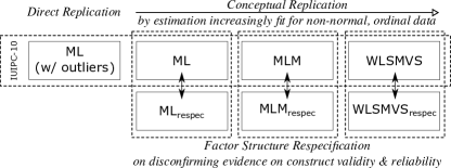
Figure 1: Analysis approach

We faced the didactic challenge that even though WLSMVS would be best suited for the task at hand [8], it is least used in the privacy community. And its probit estimation is interpreted differently to other methods. Hence, we chose to make the MLM model the primary touch stone for our analysis. It carries the advantages of being robust to moderately skewed non-normal data and of yielding interpretations natural to the community.

In our analysis process depicted in Figure 2, we used our three samples deliberately. For the factor analysis of IUIPC-10, we used base Sample B as main dataset to work with. We retained Sample A as an auxiliary sample to conduct exploratory factor analyses and to have respecification proposals informed by more than one dataset, thereby warding against the impact of chance. Sample V was reserved for validation after a final model was chosen. Figure 2 illustrate this relationship of the different samples to analysis stages.

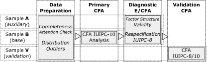
Figure 2: Which steps were taken on what sample

First, we established a sound data preparation, including consideration for measurement level and distribution as well as outliers. Second, we computed a covariance-based confirmatory factor analysis on the IUIPC-10 second-order model [45], complemented with alternative one-factor and two-factor models. This comparison served to confirm the three-dimensionality of IUIPC. We evaluated the hypothesized IUIPC-10 model on Sample B, gathering evidence for construct validity in the form of factorial validity evident in global and local fit, convergent and discriminant validity, as well as reliability.

Having found inconsistencies, we then engaged in a diagnosis and respecification stage. Therein, we also computed a parallel polychoric factor analysis and EFAs on samples A and B to re-assess the three-dimensional factor structure itself and to hunt down patterns of weaknesses. From this evaluation, we prepared a respecified IUIPC-8 which was first evaluated on Sample B. We compared the non-nested models of IUIPC-10 and IUIPC-8 with the Vuong Likelihood Ratio Test on the ML estimation. Otherwise, we compared between fit indices, focusing on an evenly weighted CAIC for non-nested comparisons.

Finally, once respecification and design decisions were settled, we entered the CFA validation stage. Therein, we compared the performance of the original IUIPC-10 and the respecified IUIPC-8 on the independent validation Sample V.

6.4 Estimator Choice

For the line of inquiry on which estimator to use, we computed three confirmatory factor analyses on the respective samples and IUIPC variants, differing in their estimators. Everything else being equal, these CFAs compared between

ML:

Standard Maximum Likelihood estimation,

MLM:

Maximum Likelihood estimation with robust standard errors and a Satorra-Bentler scaled test statistic, tailored for non-normal continuous data,

WLSMVS:

Weighted Least Square estimation with Satterthwaite means/variance adjusted test statistics, a preferred option for ordinal data.

These three estimators are increasingly better prepared to handle non-normal, ordinal data.

The comparison across estimators bears the note of caution that the estimation methods are quite different in their underlying approach and their fit measures not directly comparable. Hence, while the fit measures can show that an estimation performed well in its own right, it would stretch the interpretation to compare them across estimators.

7 Results

7.1 Sample

Table 3: Sample Refinement

Phase A B V Excl. Size Excl. Size Excl. Size Starting Sample $226$ $473$ $467$ Incomplete $0$ $226$ $58$ $415$ $34$ $433$ Duplicate $7$ $219$ $25$ $390$ $0$ $433$ FailedAC$>1$ $14$ $205$ $11$ $379$ $0$ $433$ MV Outlier $4$ $201$ $9$ $370$ $14$ $419$ Final Sample $N_{\mathsf{A}}^{\prime}=201$ $N_{\mathsf{B}}^{\prime}=370$ $N_{\mathsf{V}}^{\prime}=419$

Note: $N_{\mathsf{A}}=205$, $N_{\mathsf{B}}=379$, $N_{\mathsf{V}}=433$ are after attention checks.

Table 4: Demographics

	Overall
$N_{\mathsf{A}}$	205
Gender (%)
Female	80 (39.0)
Male	125 (61.0)
Rather not say	0 ( 0.0)
Age (%)
18-24	109 (53.2)
25-34	71 (34.6)
35-44	18 ( 8.8)
45-54	4 ( 2.0)
55-64	3 ( 1.5)
65+	0 ( 0.0)

(a) Sample A

	Overall
$N_{\mathsf{B}}$	379
Gender (%)
Female	197 (52.0)
Male	179 (47.2)
Rather not say	3 ( 0.8)
Age (%)
18-24	41 (10.9)
25-34	72 (19.0)
35-44	84 (22.2)
45-54	57 (15.0)
55-64	97 (25.6)
65+	28 ( 7.4)

(b) Sample B

	Overall
$N_{\mathsf{V}}$	433
Gender (%)
Female	217 (50.1)
Male	212 (49.0)
Rather not say	4 ( 0.9)
Age (%)
18-24	92 (21.2)
25-34	143 (33.0)
35-44	83 (19.2)
45-54	58 (13.4)
55-64	44 (10.2)
65+	13 ( 3.0)

(c) Sample V

Note: Samples B and V were drawn to be representative of the UK census by age and gender; Sample A was not.

We refined the three samples A, B and V in stages, where Table 3 accounts for the refinement process. First, we removed incomplete cases without replacement. Second, we removed duplicates across samples by the participants’ Prolific ID. Third, we removed cases in which participants failed more than one attention check ($\mathsf{FailedAC}>1$). Overall, of the $N_{\mathsf{C}}=1074$ complete cases, only $5.3\%$ were removed due to duplicates or failed attention checks.

The demographics the samples are outlined in Table 4. In samples B and V meant to be UK representative, we found a slight under-representation of elderly participants compared to the UK census age distribution. Interested readers can reproduce the ML and MLM CFA from the correlation matrices and the standard deviations of the samples included in Appendix A, DocumentVersionTRTable 17DocumentVersionConferenceTable 24b.

7.2 Data Preparation

DocumentVersionTR

7.2.1 Extreme Multi-Collinearity

While we found considerable correlation between indicator variables (cf. Appendix Table 17), there was no extreme case of multi-collinearity.

DocumentVersionTR

7.2.2 Non-Normality

We checked the input variables in all samples for indications of uni-variate non-normality. RedundantContentThe distribution histograms and density plots are available in Figure LABEL:fig:histograms in Appendix A. All input variables (of all samples) were moderately negatively skewed with the most extreme skew being $-2.09$. In general, all input variables apart from coll1 showed a positive kurtosis, less than $2.4$.

While already ordinal in measurement level (7-point Likert scales), all input items need to be considered non-normal, yet not extremely so.

DocumentVersionTR

7.2.3 Outliers

We checked for uni-variate and multivariate outliers. These checks were computed on parcels of indicator variables of 1^st-order sub-scales Control, Awareness and Collection. We checked for univariate outliers with the robust outlier labeling rule and multi-variate outliers on all three variables with the Mahalanobis distance (at a fixed threshold of $12$). We checked the sample distributions and marked outliers with 3-D scatter plots on the three variables.

All our IUIPC-10 datasets yielded $6\%$ univariate outliers by the robust outlier labeling rule and $3\%$ multi-variate outliers with a Mahalanobis distance of $12$ or greater. We removed multi-variate outliers from the samples without replacement, yielding sample sizes $N_{\mathsf{A}}^{\prime}$, $N_{\mathsf{B}}^{\prime}$, and $N_{\mathsf{V}}^{\prime}$, respectively, as indicated in Table 3.

7.3 Descriptive Statistics

We found all indicator variables of all samples to be substantively negatively skewed, meaning that there are relatively few small values and that the distribution tails off to the left [26, p. 48], with the most extreme skew being $-2.09$. In general, all indicators apart from coll1 showed a substantive positive kurtosis [36, pp. 74], that is, peakedness, less than $2.4$. While this pattern of substantive non-normality was present in the indicator distributions, we also found it in the IUIPC sub-scales and illustrate these distributions in Table 5 and Figure 3. We observed that the three samples had approximately equal distributions by sub-scales. Explicitly controlling for the difference between Samples B and V, we found that none of their sub-scale means were statistically significantly differentDocumentVersionTR:DocumentVersionConference, the maximal absolute standardized mean difference being 0.13—a small magnitude. (i) ctrl, $t(807.35)=1.08,p=.279$, $g=0.08$, 95% CI $[-0.06,0.21]$; (ii) awa, $t(801.11)=1.9,p=.058$, $g=0.13$, 95% CI $[-0.01,0.27]$; (iii) coll, $t(776.13)=-0.25,p=.802$, $g=-0.02$, 95% CI $[-0.16,0.12]$; (iv) iuipc, $t(804.51)=0.92,p=.356$, $g=0.06$, 95% CI $[-0.07,0.2]$. We are, thereby, confident that the obtained descriptive statistics in Table 5 generalize well as benchmarks for IUIPC-10 in the UK population. We observed that the standardized mean differences between IUIPC-10 and our Sample B by sub-scales were smallDocumentVersionTR: (i) ctrl: $p<.001$, $g=-0.27$, 95% CI $[-0.41,-0.13]$; (ii) awa: $p<.001$, $g=-0.4$, 95% CI $[-0.54,-0.27]$; (iii) coll: $p=.538$, $g=0.04$, 95% CI $[-0.09,0.18]$; (iv) iuipc: $p=.005$, $g=-0.2$, 95% CI $[-0.33,-0.06]$. DocumentVersionConference, with a maximum absolute standardized mean difference of 0.4. Sample B’s mean estimates of ctrl and awa were statistically significantly greater than IUIPC’s, both $p<.001$.

Our IUIPC-10 samples yielded $6\%$ univariate outliers by the robust outlier labeling rule and $3\%$ multi-variate outliers with a Mahalanobis distance of $12$ or greater [36, pp. 72].

Of the requirements for Maximum Likelihood estimation, we find the multi-variate normality violated in a case of non-continuous measurement. Our data preparation handled the outliers as recommended.

Table 5: Means (SDs) of the parceled sub-scales of IUIPC-10

Sample A Sample B Sample V Malhotra et al. ctrl $5.82$ $(0.99)$ $5.93$ $(0.78)$ $5.86$ $(0.84)$ $5.67$ $(1.06)$ awa $6.22$ $(0.78)$ $6.51$ $(0.52)$ $6.43$ $(0.66)$ $6.21$ $(0.87)$ coll $5.48$ $(1.12)$ $5.58$ $(1.12)$ $5.60$ $(1.04)$ $5.63$ $(1.09)$ iuipc $5.84$ $(0.75)$ $6.00$ $(0.61)$ $5.96$ $(0.64)$ $5.84$ $(1.01)$

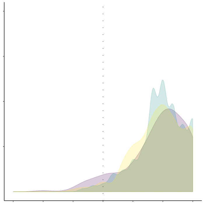
(a) Control

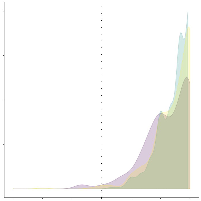
(b) Awareness

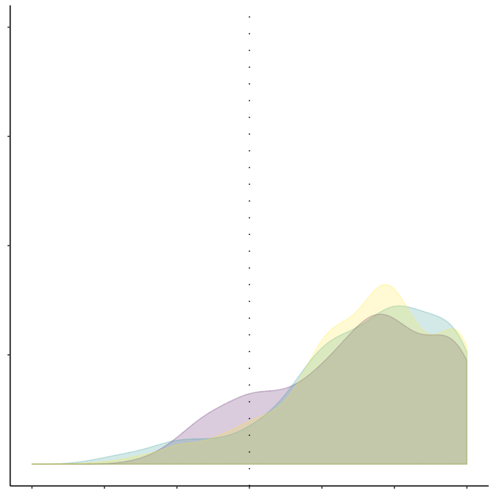
(c) Collection

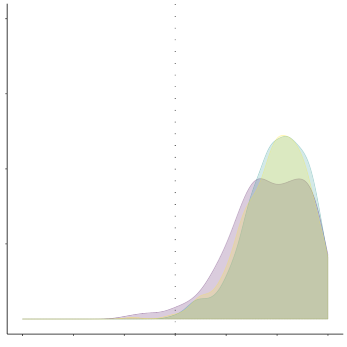
(d) IUIPC-10 Overall

Figure 3: Density of IUIPC-10 subscale responses across samples (A: violet, B: green, V: yellow). Note: All graphs are on the same scale

7.4 Construct Validity

7.4.1 Factorial Validity

To confirm the hypothesized factor structure of IUIPC-10, we computed confirmatory factor analyses on one-factor, two-factor and the hypothesized three-dimensional second-order model. We present the fit of the respective estimations in Table 19. By a likelihood-ratio $\chi^{2}$ difference test, we concluded that the two-factor solution was statistically significantly better than the one-factor solution, $\chi^{2}(1)=138.761,p<.001$. In turn, the three-factor solutions were statistically significantly better than the two-factor solution, $\chi^{2}(2)=49.957,p<.001$. We DocumentVersionTRrejected the respective hypotheses $H_{\mathsf{LRT},\chi^{2},0}$ and accepted the hypothesized three-factor second-order model, offering confirming evidence for its factorial validity.

Table 6: Comparison of different model structures of IUIPC-10 on Sample B with MLM estimationCaptionExplanations.
The models show increasingly better fits in scaled $\chi^{2}$, CFI, and CAIC, supporting the predicted hierarchical three-factor model.

One Factor Two Factors Three Factors (1^st Order) Three Factors (2^nd Order) $\chi^{2}(\mathit{df})$ 481.87 (35) 239.28 (34) 163.69 (32) 163.69 (32) $\chi^{2}/\mathit{df}$ 13.77 7.04 5.12 5.12 CFI .73 .87 .92 .92 GFI 1.00 1.00 1.00 1.00 RMSEA .19 [.17, .20] .13 [.11, .14] .11 [.09, .12] .10 [.09, .12] SRMR .14 .09 .10 .10 Scaled $\chi^{2}(\mathit{df})$ 377.87 (35) 189.71 (34) 131.42 (32) 131.42 (32) CAIC 600.572 361.941 294.264 294.264 Scaled CAIC 496.570 312.366 261.990 261.990

DocumentVersionTR

Model Overview

To further test the construct validity of the three-factor second-order model, we conducted a confirmatory factor analysis of the IUIPC-10 measurement model on Sample BDocumentVersionTR ($N_{\mathsf{B}^{\prime}}=370$).

DocumentVersionTRThe second-order model considers the indicator variables as first-level reflective measurement of the latent variables (Control, Awareness, and Collection). It further models that these first-level latent variables are caused by the second-order factor: IUIPC. We included the model’s path plot in Figure 7. DocumentVersionConferenceWe included the model’s path plot in Figure 7 in Appendix LABEL:app:validity.

DocumentVersionTR

Figure 4: CFA paths plot with standardized estimates of IUIPC-10 on Sample B. Note: The coefficients are standardized

Global Fit

Our first point of call for further evaluating the factorial validity of IUIPC-10 is is global fit. We included an overview of the fit measures on different samples in Table 10, drawing attention to the top row.

First, we observed that the exact-fit test failed for IUIPC-10 irrespective of estimator, that is, the exact-fit null hypotheses $H_{\chi^{2},0}$ were rejected with the $\chi^{2}$-tests being statistically signficant. For the RMSEA-based hypotheses we have: (i) The close-fit test evaluating whether RMSEA is likely less or equal $.05$ failed irrespective of estimator. (ii) The not-close-fit test could not be rejected for either estimator, withholding support for the models. (iii) Finally, the poor-fit test could not be rejected either for any models, with the upper bound of the RMSEA CI being greater than or equal as $.10$, indicating a poor fit.

The fit indices CFI and SRMR yielded $.92$ and $.10$ for the ML based models, respectively, not supporting the models. None of the models passed the $\mathit{HBR}$ combination rule used by Malhotra et al. The direct replication of IUIPC with ML estimation and outliers present fared more poorly than the corresponding ML models implementing the stated assumption: $\chi^{2}(32)=202.789,p<.001$; CFI=$.90$; RMSEA=$.12$ $[.10,.13]$; SRMR=$.11$; CAIC=333.8.

Overall, we conclude that the global fit of the model was poor and that we found disconfirming evidence for IUIPC-10’s factorial validity. This disconfirmation of the CFA held irrespective of the data preparation and estimator employed. Our further examination of construct validity will be on the touch-stone MLM model.

Local Fit

We analyzed the correlation and standardized covariance residuals of the MLM model presented in Table 29 on page 29.

First, we observed that the correlation residuals in Table 29a showed a number of positive correlations greater than $.10$. We noticed especially that there were patterns of residual correlations with ctrl3 and awa3. Second, we saw in Table 29b that there were a majority of statistically significant residual standardized covariances, indicating a wide-spread poor local fit and a repetition of the pattern seen in the correlations. These statistically significant residuals were too frequent to be attributed to chance alone. Positive covariance residuals were large and prevalent, which showed that—in many cases—the CFA model underestimated the association between the variables present in the sample.

From from the positive covariance residuals with awa and coll indicators, we concluded that ctrl3 misloaded both on factors Awareness and Collection. From the positive covariance residuals between awa3 and the coll variables, we inferred that this indicator loaded on the factor Collection. These observations yielded further disconfirming evidence for the factorial validity of IUIPC-10, especially regarding the unidimensionality of its sub-scales. The correlation residuals showed patterns of positive correlations greater than $.10$ with ctrl3 and awa3, matched with statistically significant standardized covariances. This indicated considerable misloading on these indicators and disconfirmed the unidimensionality of the corresponding sub-scales.

7.4.2 Convergent and Discriminant Validity

We first analyzed the standardized loadings and the variance explained in Table 7. Therein, we found that ctrl3 and awa3 only explained $.17$ and $.20$ of the variance, respectively. Those values were unacceptably below par ($R^{2}>.50$), yielding a poor convergent validity.

Table 7: Factor loadings and their standardized solution of the MLM CFA of IUIPC-10 on Sample BCaptionExplanations.
We find sub-par standardized loadings $\beta<.70$ for ctrl3 and awa3, yielding a poor variance extracted $R^{2}\leq.20$ and, thereby, low $\mathit{AVE}<.50$ for control and awareness, indicating sub-par internal consistency. The equally sub-par construct reliability $\omega<.70$ yields a low signal-to-noise ratio less than $2$.

Factor	Indicator	Factor Loading				Standardized Solution				Reliability
		$\lambda$	$\mathit{SE}_{\lambda}$	$Z_{\lambda}$	$p_{\lambda}$	$\beta$	$\mathit{SE}_{\beta}$	$Z_{\beta}$	$p_{\beta}$	$R^{2}$	$\mathit{AVE}$	$\alpha$	$\omega$	$\mathit{S/\!N}_{\omega}$
ctrl	ctrl1	$1.00^{+}$				0.73	0.05	15.14	$<.001$	0.54	0.40	0.62	0.66	1.92
	ctrl2	$1.00\phantom{{}^{+}}$	0.11	8.76	$<.001$	0.73	0.05	13.73	$<.001$	0.53
	ctrl3	$0.59\phantom{{}^{+}}$	0.11	5.36	$<.001$	0.41	0.06	6.89	$<.001$	0.17
aware	awa1	$1.00^{+}$				0.74	0.05	15.36	$<.001$	0.54	0.39	0.64	0.66	1.92
	awa2	$1.13\phantom{{}^{+}}$	0.13	8.53	$<.001$	0.81	0.04	18.45	$<.001$	0.66
	awa3	$0.90\phantom{{}^{+}}$	0.14	6.64	$<.001$	0.44	0.05	8.83	$<.001$	0.20
collect	coll1	$1.00^{+}$				0.81	0.02	38.77	$<.001$	0.66	0.72	0.91	0.91	10.13
	coll2	$0.76\phantom{{}^{+}}$	0.05	14.86	$<.001$	0.76	0.04	20.99	$<.001$	0.58
	coll3	$1.06\phantom{{}^{+}}$	0.04	23.63	$<.001$	0.94	0.01	70.89	$<.001$	0.88
	coll4	$0.95\phantom{{}^{+}}$	0.05	18.14	$<.001$	0.86	0.03	33.94	$<.001$	0.74
iuipc	collect	$0.41\phantom{{}^{+}}$	0.08	5.42	$<.001$	0.37	0.07	5.57	$<.001$	0.14
	ctrl	$0.42\phantom{{}^{+}}$	0.07	6.05	$<.001$	0.61	0.09	6.47	$<.001$	0.38
	aware	$0.36\phantom{{}^{+}}$	0.06	6.40	$<.001$	0.89	0.11	8.06	$<.001$	0.79
Note: + fixed parameter; the standardized solution is STDALL

DocumentVersionTRWhile we assessed the intra- and inter-factor correlations [6], let focus here on the criteria specified in Section 2.2.2. In terms of convergent validity, we evaluated the Average Variance Extracted (AVE) and Composite Reliability (CR) $\omega$ in Table 7. While the CR $\omega$ being greater than the AVE for all three dimensions indicated support, we observed that the AVE being less than $.50$ for both Control and Awareness, showing that there is more error variance extracted than factor variance. Similarly, $\omega<.70$ implied sub-par convergent validity.

For discriminant validity, we found the Fornell-Larcker and HTMT-criteria fulfilled, offering support for the specified models.

7.5 Reliability: Internal Consistency

DocumentVersionTRWe summarized a range of item/construct reliability metrics of main Sample B in Table 8, observing that Guttman’s $\lambda_{6}$ dropped to less than $.6$ and that the average correlation for Control and Awareness were low.

Let us consider the reliability criteria derived from the MLM CFA model in Table 7. Considering Cronbach’s $\alpha$, we observed estimates for Control and Awareness less than the $.70$, what Nunnally classified only acceptable to “save time and energy.” The Composite Reliability estimate $\omega$ was equally sub-par.

DocumentVersionTR

Table 8: Item/construct reliability metrics of IUIPC-10 on Sample B

Construct	$\alpha$	$\mathsf{LL}(\alpha)$	$\mathsf{UL}(\alpha)$	$\lambda_{6}$	$\mathsf{avg}(r)$	$r_{\mathsf{i/w}}$	Bartlett $p$	KMO	MSA
Control	0.63	0.57	0.68	0.56	0.36		$<.001$	0.59
ctrl1						0.79			0.56
ctrl2						0.80			0.56
ctrl3						0.69			0.76
Awareness	0.68	0.64	0.73	0.62	0.42		$<.001$	0.60
awa1						0.77			0.57
awa2						0.77			0.57
awa3						0.78			0.79
Collection	0.91	0.89	0.92	0.89	0.71		$<.001$	0.83
coll1						0.89			0.88
coll2						0.83			0.88
coll3						0.93			0.77
coll4						0.89			0.81

7.6 Respecification

In face of the disconfirming evidence discovered on construct validity, we decided to remove the items ctrl3 and awa3 from the scale, at the risk of losing identification. We compared the non-nesteds models IUIPC-10 and IUIPC-8 with the Vuong test on the ML estimation. The variance test indicated the two models as distinguishable, $\omega^{2}=1.926$, $p<.001$. The Vuong non-nested likelihood-ratio test rejected the null hypothesis that both models were equal. The IUIPC-8 model fitted statistically significantly better than the IUIPC-10 model, LRT $z=-34.541$, $p<.001$. Table 10 illustrates the comparison of the two models. This consitutes evidence of the factorial validity of the revised scale, including a confirmation of the unidimensionality of its sub-scales.

7.7 Respecification

One possibility to handle the situation is to specify explicitly in the measurement model of IUIPC-10 that ctrl3 and awa3 are indicators to multiple factors. While this approach could offer a better overall fit, the IUIPC-10 scale would still suffer from poor convergent and discriminant validity.

We can advocate to remove ctrl3 and awa3 from the scale and create a reduced IUIPC-8 scale instead. Clearly, such a step comes at a price. In CFA, the possible dire price lies in the loss of identification. Kelly’s rule of thumb on number of indicators states: “Two might be fine, three is better, four is best, and anything more is gravy.”

Ideally, to be identified in a nonstandard CFA model, for each factor there should be at least three indicators with mutually uncorrelated errors. For Control and Awareness, we are running the risk of violating this rule of identification. However, with a two-indicator situation as presented here, we could reach identification if their errors are uncorrelated within them and they are not correlated with the error of another factor.

We compared the non-nested pair IUIPC-10 and IUIPC-8 with the Vuong test on the ML estimation. The variance test indicated the two models as distinguishable, $\omega^{2}=1.926$, $p<.001$. The Vuong non-nested likelihood-ratio test rejected the null hypothesis that both models are equal for the focal population. The IUIPC-8 model fits statistically significantly better than the IUIPC-10 model, LRT $z=-34.541$, $p<.001$. We display the comparison of IUIPC-10 and the trimmed model in Table 10. This is strong evidence of the factorial validity of the revised scale, including a confirmation of the unidimensionality of its sub-scales.

While the IUIPC-8 model yields a significantly better fit, there are still two significant standardized residuals with appreciable negative correlations of concern: between coll1 and awa1/awa2, respectively. The negative covariance residual means that the model overestimates the covariances between the first collection item and the awareness items.

Remark 1 (Correlated errors).

We inspected the questionnaire itself for evidence of method correlation (cf. Appendix A). We found specifically that coll1 and coll3 follow a parallel construction with the stem “It bothers me…,” which could lead to correlated error variances on substantive grounds. Testing the this variant with an LRT difference test on nested models, we found that the difference is statistically significant in the ML estimation, but not under Satorra-Bentler correction, $\chi^{2}(1)=3.975,p=.046$ and $\chi^{2}(1)=2.548,p=.110$, respectively. The difference between the variants is even less pronounced under WLSMVS estimation. Hence, we choose to keep the model without correlated errors.

The respecification is still highly correlated with IUIPC-10: (i) ctrl, $r=.91$, 95% CI $[.89,.93]$; (ii) awa, $r=.86$, 95% CI $[.83,.88]$; (iii) iuipc, $r=.96$, 95% CI $[.96,.97]$, all statistically significant at $p<.001$, giving us evidence for IUIPC-8’s concurrent validity.

Table 9: Respecification of IUIPC-10 to IUIPC-8 on Sample BCaptionExplanations.
All IUIPC-10 models failed the poor-fit tests irrespective of estimator. The respecified IUIPC-8 yielded a statistically significantly better fit by the Vuong test on the ML estimation, with better CAIC throughout. The $\mathsf{RMSEA}$ on IUIPC-8 still asks us to mind the residuals.

Instrument	Respecification	Estimator
		ML	MLM‡	WLSMVS‡
IUIPC-10		$\chi^{2}(32)=163.691,p<.001$	$\chi^{2}(32)=131.417,p<.001$	$\chi^{2}(15)=181.149,p<.001$
		CFI=$.92$; GFI=$1.00$	CFI=$.92$; GFI=$1.00$	CFI=$.95$; GFI=$.99$
		RMSEA=$.11$ $[.09,.12]$	RMSEA=$.10$ $[.08,.12]$	RMSEA=$.17$ $[.15,.19]$
		SRMR=$.10$; CAIC=294.3	SRMR=$.10$; CAIC=262	SRMR=$.10$; CAIC=414.6
		$\uparrow$	$\uparrow$	$\uparrow$
	Trim ctrl3 & awa3	$\Delta{\mathsf{CFI}}=0.05$; $\Delta{\mathsf{CAIC}}=-132.57$	$\Delta{\mathsf{CFI}}=0.05$; $\Delta{\mathsf{CAIC}}=-112.32$	$\Delta{\mathsf{CFI}}=0.04$; $\Delta{\mathsf{CAIC}}=-191.39$
		Vuong LRT $z=-34.541$, $p<.001$
		$\downarrow$	$\downarrow$	$\downarrow$
IUIPC-8		$\chi^{2}(17)=54.863,p<.001$	$\chi^{2}(17)=42.836,p<.001$	$\chi^{2}(10)=33.282,p<.001$
		CFI=$.97$; GFI=$1.00$	CFI=$.98$; GFI=$1.00$	CFI=$.99$; GFI=$1.00$
		RMSEA=$.08$ $[.06,.10]$	RMSEA=$.07$ $[.05,.10]$	RMSEA=$.08$ $[.04,.12]$
		SRMR=$.03$; CAIC=161.7	SRMR=$.03$; CAIC=149.7	SRMR=$.04$; CAIC=223.2

Note: ^‡ Robust estimation with scaled test statistic. $\mathsf{RMSEA}$ reported wih 90% CI.

Table 10: Respecification of IUIPC-10 to IUIPC-8 on Sample B

Instrument & Estimator Respecification ML MLM^‡ WLSMVS^‡ IUIPC-10 $\chi^{2}(32)=163.691,p<.001$ $\chi^{2}(32)=131.417,p<.001$ $\chi^{2}(15)=181.149,p<.001$ CFI=$.92$; GFI=$1.00$ CFI=$.92$; GFI=$1.00$ CFI=$.95$; GFI=$.99$ RMSEA=$.11$ $[.09,.12]$ RMSEA=$.10$ $[.08,.12]$ RMSEA=$.17$ $[.15,.19]$ SRMR=$.10$; CAIC=294.3 SRMR=$.10$; CAIC=262 SRMR=$.10$; CAIC=414.6 $\uparrow$ $\uparrow$ $\uparrow$ Trim ctrl3 & awa3 $\Delta{\mathsf{CFI}}=0.05$; $\Delta{\mathsf{CAIC}}=-132.57$ $\Delta{\mathsf{CFI}}=0.05$; $\Delta{\mathsf{CAIC}}=-112.32$ $\Delta{\mathsf{CFI}}=0.04$; $\Delta{\mathsf{CAIC}}=-191.39$ Vuong LRT $z=-34.541$, $p<.001$ $\downarrow$ $\downarrow$ $\downarrow$ IUIPC-8 $\chi^{2}(17)=54.863,p<.001$ $\chi^{2}(17)=42.836,p<.001$ $\chi^{2}(10)=33.282,p<.001$ CFI=$.97$; GFI=$1.00$ CFI=$.98$; GFI=$1.00$ CFI=$.99$; GFI=$1.00$ RMSEA=$.08$ $[.06,.10]$ RMSEA=$.07$ $[.05,.10]$ RMSEA=$.08$ $[.04,.12]$ SRMR=$.03$; CAIC=161.7 SRMR=$.03$; CAIC=149.7 SRMR=$.04$; CAIC=223.2

Note: ^‡ Robust estimation with scaled test statistic.

DocumentVersionTRWe included the path model for the MLM estimation on Sample B in Figure 10. We put the corresponding residuals table in Table 32 on page 32. DocumentVersionTR

Figure 5: CFA paths plot with standardized estimates of the respecified IUIPC-8 on Sample B. Note: The coefficients are standardized

DocumentVersionTR

Table 11: Factor loadings and their standardized solution of the MLM CFA of IUIPC-8 on Sample BCaptionExplanations.
The standardized factor loadings $\beta$ are largely greater than $.70$, yielding satisfactory $\mathit{AVE}>.50$. The construct reliability $\omega>.70$ passes the threshold for control and awareness yielding moderate signal-to-noise ratios; the reliability of collection is excellent.

Factor	Indicator	Factor Loading				Standardized Solution				Reliability
		$\lambda$	$\mathit{SE}_{\lambda}$	$Z_{\lambda}$	$p_{\lambda}$	$\beta$	$\mathit{SE}_{\beta}$	$Z_{\beta}$	$p_{\beta}$	$R^{2}$	$\mathit{AVE}$	$\alpha$	$\omega$	$\mathit{S/\!N}_{\omega}$
ctrl	ctrl1	$1.00^{+}$				0.76	0.06	13.40	$<.001$	0.57	0.56	0.72	0.72	2.52
	ctrl2	$0.98\phantom{{}^{+}}$	0.14	7.01	$<.001$	0.74	0.06	11.58	$<.001$	0.54
aware	awa1	$1.00^{+}$				0.69	0.05	13.45	$<.001$	0.48	0.64	0.76	0.78	3.55
	awa2	$1.33\phantom{{}^{+}}$	0.18	7.33	$<.001$	0.90	0.05	17.34	$<.001$	0.80
collect	coll1	$1.00^{+}$				0.81	0.02	39.01	$<.001$	0.66	0.72	0.91	0.91	10.13
	coll2	$0.76\phantom{{}^{+}}$	0.05	14.83	$<.001$	0.76	0.04	20.90	$<.001$	0.58
	coll3	$1.06\phantom{{}^{+}}$	0.04	23.67	$<.001$	0.94	0.01	70.72	$<.001$	0.88
	coll4	$0.95\phantom{{}^{+}}$	0.05	18.15	$<.001$	0.86	0.03	33.67	$<.001$	0.74
iuipc	collect	$0.34\phantom{{}^{+}}$	0.08	4.28	$<.001$	0.31	0.07	4.31	$<.001$	0.09
	ctrl	$0.39\phantom{{}^{+}}$	0.08	4.90	$<.001$	0.56	0.11	5.01	$<.001$	0.31
	aware	$0.33\phantom{{}^{+}}$	0.07	4.99	$<.001$	0.86	0.14	6.03	$<.001$	0.74
Note: + fixed parameter; the standardized solution is STDALL

DocumentVersionTR

Table 12: Evidence for discriminant validity of IUIPC-10 (Fornell-Larcker Criterion and Heterotrait-Monotrait Ratio) on Sample BCaptionExplanations.
The Fornell-Larcker criterion of $\sqrt{\mathit{AVE}}$ greater than any correlation with any other factor and the $\mathit{HTMT}<.85$ are fulfilled.

	1	2	3	4
1. ctrl	0.634
2. aware	0.546	0.627
3. collect	0.227	0.329	0.848
4. iuipc	0.613	0.891	0.37	0.769
Note: The diagonal contains the $\sqrt{\mathit{AVE}}$

(a) Fornell-Larcker

	1	2	3
1. ctrl	—
2. aware	0.67	—
3. collect	0.32	0.45	—

(b) HTMT Ratio

7.8 Validation

We validated the respecified IUIPC-8 model on the independent validation sample V and compared against he performance of IUIPC-10. We offered this comparison under consideration of all three estimators in Table 23.

First, we observed under ML estimation that the two models are indeed statistically significantly distinguishable with the variance test, $\omega^{2}=2.489$, $p<.001$. Furthermore, applied to the validation sample V, IUIPC-8 was the statistically significantly better model according to the Vuong test, LRT $z=-34.541$, $p<.001$.

For IUIPC-10 on V, we noticed that the ML estimation failed all test criteria, incl. the poor-fit hypothesis with a $\hat{\epsilon}=.08$ and $\hat{\epsilon}_{\mathsf{UL}}\geq.10$. The residuals showed a similar pattern as on Sample B. Again, the direct replication of IUIPC with outliers showed a poorer fit than the other ML estimations: $\chi^{2}(32)=137.368,p<.001$; CFI=$.93$; RMSEA=$.09$ $[.07,.10]$; SRMR=$.09$; CAIC=270.5.

The respecified IUIPC-8 fared better. Here, the ML estimator already offered a good fit. The estimators, MLM and WLSMVS, performed equally well, if not better.

Overall, we concluded that IUIPC-8 could be validated on an independent dataset as a well fitting model, whereas IUIPC-10 was disconfirmed once more.

Table 13: Comparison of IUIPC-10 and IUIPC-8 on Validation Sample V

Instrument & Estimator Respecification ML MLM^‡ WLSMVS^‡ IUIPC-10 $\chi^{2}(32)=122.015,p<.001$ $\chi^{2}(32)=80.69,p<.001$ $\chi^{2}(16)=151.118,p<.001$ CFI=$.94$; GFI=$1.00$ CFI=$.95$; GFI=$1.00$ CFI=$.96$; GFI=$.99$ RMSEA=$.08$ $[.07,.10]$ RMSEA=$.07$ $[.05,.09]$ RMSEA=$.14$ $[.12,.16]$ SRMR=$.08$; CAIC=254.6 SRMR=$.08$; CAIC=213.3 SRMR=$.07$; CAIC=404.3 $\uparrow$ $\uparrow$ $\uparrow$ Trim ctrl3 & awa3 $\Delta{\mathsf{CFI}}=0.05$; $\Delta{\mathsf{CAIC}}=-111.6$ $\Delta{\mathsf{CFI}}=0.05$; $\Delta{\mathsf{CAIC}}=-82.76$ $\Delta{\mathsf{CFI}}=0.04$; $\Delta{\mathsf{CAIC}}=-174.5$ Vuong LRT $z=-35.146$, $p<.001$ $\downarrow$ $\downarrow$ $\downarrow$ IUIPC-8 $\chi^{2}(17)=34.532,p=.007$ $\chi^{2}(17)=22.04,p=.183$ $\chi^{2}(10)=24.844,p=.005$ CFI=$.99$; GFI=$1.00$ CFI=$.99$; GFI=$1.00$ CFI=$.99$; GFI=$1.00$ RMSEA=$.05$ $[.03,.07]$ RMSEA=$.03$ $[.00,.07]$ RMSEA=$.06$ $[.03,.09]$ SRMR=$.03$; CAIC=143 SRMR=$.03$; CAIC=130.6 SRMR=$.03$; CAIC=229.8

Note: ^‡ Robust estimation with scaled test statistic.

7.9 Summary

The construct validity of IUIPC according to RQ 1 bears a deliberate discussion. On the one hand, we could confirm the three-dimensionality and second-order model Malhotra et al. [45] postulated. On the other hand, factorial validity evidenced in global and local fit—especially the unidimensionality of the first-order factors Control and Awareness—does not seem to be given neither on the main Sample B nor on the validation Sample V. The convergent validity and reliability of these sub-scales is equally in question, our estimates having been lower than Malhotra et al.’s.

7.10 Estimator Appraisal

While we have already shown estimator invariance according to RQ 2 throughout confirmation and validation, we are now turning to the question of estimator viability asked in RQ 3.

Considering the viability of each estimator in their own right, ML without outlier treatment showed the worst performance of the ML-based estimations. We would discourage its use. Let us consider the remaining estimations with outlier treatment. Comparing between ML and MLM, both estimators behaved similarly on the relative changes between the misspecified IUIPC-10 and the respecified IUIPC-8. MLM consistently offered the stronger fit.

Even though robust WLS is estimating more parameters (loadings, errors, thresholds) than its ML counterparts, we still believe it is fair to say that WLSMVS seemed most sensitive to the misspecification of IUIPC-10. On both samples, we observed a great improvement of fit indices when comparing between the WLSMVS IUIPC-10 and IUIPC-8 models. Hence, the robust WLS estimation is certainly viable in its own right, in fact, we would consider it quite robust against Type I errors.

Having assessed MLM and WLSMVS as face-viable on their global fit, let us further appraise their model interpretations and mean structures. For this inquiry, we follow the reasoning of Bovaird and Koziol [8, pp]. Let us train our lens on a single indicator for illustration: awa2. Here, the MLM estimation tells us that individuals with average levels of Awareness will have an expected response on item awa2 of $6.62$. Of course, this value does not exist on the 7-point Likert scale. For each increase of one unit of Awareness, we would expect awa2 to increase by $1.13$ points. For a single unit of increase from the mean, the prediction $7.75$ is obviously out-of-bounds of the scale, hence, an invalid prediction. This phenomenon is an artifact of ML-based estimation on heavily non-normal, ordinal data.

Following the same line of inquiry for the robust WLS estimation, these issues do not exist. Here, the loading of awa2 $\lambda_{\mathsf{awa2}}=1.07$ indicates the expected change of the probit of an individuals’s response to awa2. Under this estimation, an Awareness of $-1.88$ is required to choose response option 6–“Agree” with a likelihood of 50%; of $-0.4$ for option 7–“Strongly Agree” with a likelihood of 50%. Clearly, the robust WLS prediction of the individual’s choice yields a more informative model.

Hence, considering this qualitative appraisal of both estimation methods, MLM and robust WLS, we find that the robust WLS estimation has appreciable advantages in model interpretation. While arguments over probit and likelihoods might be less common in the privacy community than the straight-forward MLM factor loading interpretations, the robust WLS method could offer the community more information how a users really endorse options of a privacy concern scale, such as IUIPC.

Table 14: Selected evidence for construct validity and reliability criteria on Samples B and V under MLM estimationCaptionExplanations.
The factorial validity shows IUIPC-10 consistently failing fit measures; IUIPC-8 fared better, especially on the validation sample V. The convergent validity of IUIPC-10 is evidenced to be consistently flawed; IUIPC-8 showed suitable results, where some standardized loadings $\beta$ were shown to be border-line without violating $\mathit{AVE}>.50$. Divergent validity of IUIPC-10 suffers from the low $\mathit{AVE}$; IUIPC-8 fulfills all requirements. IUIPC-10 fails the requirements on internal consistency, especially $\omega>.70$; IUIPC-8 passes them.

		Construct Validity							Reliability
		Factorial			Convergent		Divergent		Internal Consistency
		$H_{\chi^{2},0}$	$H_{\hat{\varepsilon}\leq.05,0}$	$\mathit{HBR}$	$\beta>.70$	$\mathit{AVE}>.50$	$\sqrt{AVE}>\forall\bar{r}$	$\mathit{HTMT}<.85$	$\alpha>.70$	$\omega>.70$
IUIPC-10	B	○	○	○	○	○	DocumentVersionTR◐DocumentVersionConference◐	DocumentVersionTR●DocumentVersionConference●	○	○
	V	○	○	○	DocumentVersionTR○DocumentVersionConference○	DocumentVersionTR○DocumentVersionConference○	DocumentVersionTR○DocumentVersionConference○	DocumentVersionTR●DocumentVersionConference●	DocumentVersionTR○DocumentVersionConference○	DocumentVersionTR○DocumentVersionConference○
IUIPC-8	B	○	○	○	◐	●	DocumentVersionTR●DocumentVersionConference●	DocumentVersionTR●DocumentVersionConference●	●	●
	V	●	●	●	DocumentVersionTR◐DocumentVersionConference◐	DocumentVersionTR●DocumentVersionConference●	DocumentVersionTR●DocumentVersionConference●	DocumentVersionTR●DocumentVersionConference●	DocumentVersionTR●DocumentVersionConference●	DocumentVersionTR●DocumentVersionConference●

Note: $\mathit{HBR}$ = Hu and Bentler combination rule used by Malhotra et al. [45]; $\beta$ = standardized loading; $\mathit{AVE}$ = Average Variance Extracted; $\bar{r}$ = correlation with other factor; $\mathit{HTMT}$ = Heterotrait-Monotrait Ratio; $\omega$ = Composite Reliability.

8 Discussion

8.1 IUIPC-10 could not be confirmed

While we could attest to the strengths in content validity and the three-dimensionality of IUIPC-10, its CFA revealed a range of weaknesses in its construct validity (cf. Table 14): (i) we could not confirm factorial validity in terms of global fit, meaning that the corresponding models do not approximate the corresponding observations well; (ii) the inspection of the residuals showed an unsatisfactory local fit for two items of the sub-scales of Control and Awareness calling the the unidimensionality of these sub-scales into question. (iii) we found disconfirming evidence on the convergent validity. We further observed a sub-par reliability of the sub-scales Control and AwarenessDocumentVersionTR with a signal-to-noise ratio of $1.94$. As these assessments held true on main and validation samples, irrespective of estimators used, they offer disconfirming evidence against the scale itself.

For privacy researchers, the issues in construct validity mean that the IUIPC-10 scale shows weaknesses in measuring its hidden construct information privacy concern. The observed sub-par reliability means that IUIPC-10 measurements are contaminated by error variance, which entails a low signal-to-noise ratio and can lead to spurious and erratic results.

8.2 IUIPC-8 asserts a stronger validity

With IUIPC-8, we proposed a refined version of IUIPC that performed consistently well in terms of construct validity and reliability. We give an overview of a range of criteria in Table 14. In terms of factorial validity, we observed good global and local fits. Criteria for convergent and discriminant validity were fulfilled consistently. The respecified scale also showed appreciable improvements in reliability, yielding a 33% to 82% better signal-to-noise ratio for Awareness and Control, respectively.

We encourage privacy researchers consider carefully: On the one hand, the 10-item version of IUIPC contains more privacy concern information they will care about. It has at least three items per factor and, thereby, creates favorable conditions for CFA model identification and more robust estimation of the true value of the latent factors. However, given that two items seem to misload to a considerable degree and show low reliability, those items may confound the model. The tight fit we obtained for the 8-item version of IUIPC is encouraging: it will approximate the data well and yield sound measurement models for subsequent analysis. The strong concurrent validity with IUIPC-10 further supports using the respecified scale.

Given the evidence in this study, we endorse adopting IUIPC-8 as a brief questionnaire for Internet users’ privacy concerns.

8.3 Questionnaire wording as culprit

While our reviews of IUIPC in Section 4 asserted a sound content validity, we equally found evidence for biases rooted in the questionnaire wording. Our analysis of the distributions of IUIPC-10 and its sub-scales from Section 7.3, especially, the distribution graphs in Figure 3 showed a substantial negative skew and positive kurtosis. This seems to confirm our observation that the use of loaded words incl. “privacy” and “autonomy” may create a systematic bias through priming, further aggravated by leading questions. All these observations point towards the instrument itself influencing the respondents towards agreement.

IUIPC also suffers from multiple instances of question wording yielding nondifferentiation. While the entire questionnaire can be subject to straightlining due to the absence of reverse-coded items, we believe that items ctrl3 and awa3 were especially impacted because of the presence of double-barreled constructions. This observation could further explain why these two items showed such a low reliability and why they needed to be removed altogether.

For privacy researchers, these observations stress the importance of inspecting the question wording of instruments carefully and to assess them against commonly known biases [52, 14].

We noticed that the two items yielding a low variance explained exhibited a common structure:

ctrl3:

“I believe that online privacy is invaded when control is lost or unwillingly reduced as a result of a marketing transaction.”

awa3:

“It is very important to me that I am aware and knowledgeable about how my personal information will be used.”

They are both double-clause formulations. Item ctrl3 exhibits a disjunction (“control is lost or unwillingly reduced”) while item awa3 exhibits a conjunction (“I am aware and knowledgeable”). In terms of classical questionnaire formulation biases, they make for double-barreled questions [14], that is, asking two questions in one. Those constructions make it difficult for the respondent to know what part to answer and how to behave if only one of the clauses is fulfilled. In addition, ctrl3 contextualizes the item on “a marketing transaction,” a profession’s term which is not necessarily well-defined for the general public. Given these observations, we believe that our quantitative results are rooted in a substantive problem in the underlying questions that cause an appreciable bias and low validity.

8.4 How to use IUIPC

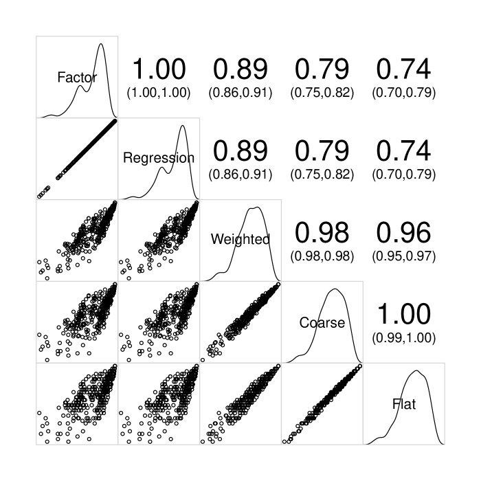
Figure 6: Relation of the IUIPC-10 factors to approximate scoresCaptionExplanations.
While allowing for factor-analysis models also yielding estimates, overall, naïve score computations, such as flat averaging, lose information over more sophisticated factor scores.

Our analysis has a range of implications for privacy researchers, not just for the use of IUIPC but any multi-dimensional privacy concern scale. First, let us consider judging IUIPC scores for a sample. Given the evidence that the instrument seems to bias responses towards agreement, it is invalid to call a particular sample “especially privacy-sensitive,” should the mean IUIPC score be greater than 4–“Neither agree nor disagree.”

Because IUIPC-10 exhibits a sub-standard reliability, privacy researchers need to be conscious a low signal-to-noise ratio. The error variance will mask the information about the respondents’ true score on IUIPC.

The most important consequence of the low reliability for privacy researchers will be the expected attenuation of relations to other latent factors [55], that is, the magnitude of effects of IUIPC-measured privacy concern on other variables, say behavior, will be reduced. This means that it will be more difficult to show the impact of privacy concern—even if the true relation between the latent variables is substantive.

Privacy researchers focusing on simple statistical tools, such as linear regressions on parceled sub-scale scores, are most affected by these shortcomings: the error variance is folded into the scores they use, masking the signal. For these researchers, IUIPC-8 offers considerable advantages by offering stronger validity and reliability. It comes at the price of eliminating two concern-items the researchers might care about. Considering the comparison of score approximations with the CFA-estimated factor in Figure 6, we assert that such privacy researchers would be worst off ignoring the factor structure altogether by simply averaging all items of IUIPC into one “flat” score ($r=.74$). It is usually better to take into account the structure, the simplest approach averaging the sub-scale scores into a “coarse” factor score. They could further improve their approximation by computing factor scoresDocumentVersionTR [18, 25], for instance “weighted” by factor loadings ($r=.89$) or linearly combined with CFA-derived “regression” coefficients. While there is a great deal of discussion on correct and incorrect uses of those factor scores, a common pragmatic approach computes a weighting by the factor loading.

Privacy researchers using advanced tools, such as confirmatory factor analysis or latent-variable structural equation modeling, need to consider a different trade-off. Of course, the analysis of the measurement model will estimate the error variance and establish the loading of each indicator on the corresponding latent factor. Hence, the contamination by error variance is somewhat contained. However, the problematic construct validity of IUIPC-10 will affect their studies, largely visible in sub-par global and local fit. They might discover their measurement model misspecified and their structural models suffering. For them, IUIPC-8 offers a better construct validity, especially useful for investigating sizable latent variable models in relation to investigations of the privacy paradox.

In terms of choice of estimators for CFA and SEM, privacy researchers can viably opt for robust WLS as an estimator tailored to the non-normal, ordinal distributions of IUIPC indicators. As we have shown, a robust WLS estimation on IUIPC-8 offers a good fit at considerable sample sizes. While the privacy community might not be accustomed to the interpretation of these probit models, they offer better model interpretability than the ML or MLM estimations. If privacy researchers decide against robust WLS, we would still advocate using a robust ML estimation (such as MLM or MLR) after a careful data preparation. DocumentVersionConferenceThe extended ArXiv version of this paper includes further considerations on design decisions.

8.5 Design decisions matter

McDonald [47] called structural modeling “the art of approximation.” In our analysis, we considered common design decisions researchers must take to gain sound approximations of reality: (i) accounting for measurement level and distribution, (ii) accounting for uni- and multi-variate outliers, and (iii) choosing an appropriate estimator for the situation at hand are among their numbers. While we included these dimensions explicitly to ward our analysis against confounding factors, we gained evidence on the sound use of scales like IUIPC for rigorous research.

First, we sound a note of caution: “Check…and check again!” Just because an instrument shows decent internal consistency measures in its conceptive study (e.g., the popular Cronbach’s $\alpha$), this does not guarantee in itself that the instrument will be valid or perform well. Of course, a prudent researcher may refer to independent confirmations of candidate instruments, but those are few and far between in our field. In our opinion, it is sage advise to create complex models in the two-step approach [2]: diligently evaluating a confirmatory factor analysis of the measurement model first, before continuing to structural or regression analyses.

We could shed light on the fact that the design decision researchers make matter. Were distribution properties checked? Outliers? Were estimators chosen that excel at the given measurement level and distribution? Fitting a model on non-normal, ordinal, outlier-prone data—such as found in IUIPC-10—relying on Maximum Likelihood (ML) estimation and hoping for the best does not seem to be a prudent way forward. Not only can this yield a poor fit but these different violations of assumptions and requirements can conspire to create seemingly well-fitting “results” that do not offer a sound approximation of reality. Those Type-I errors can well haunt a field for years to come.

Given this discussion, we would be so bold to recommend for the evaluation of measurement models:

1. employ a two-step modeling approach [2],

2. do your homework in terms of data preparation [46] and outlier handling [64],

3. choose an appropriate estimation method for the measurement level and distribution at hand [35],

4. specifically for ordinal Likert scales with expected non-normality, chose a robust estimator, such as WLSMVS DocumentVersionConference[17, 20, 8]DocumentVersionTR[51, 17, 20, 8],

5. do not just rely on global fit indices, but explicitly check and report residuals [36], and finally

6. let invariable respecification efforts be guided by substantive arguments.

These recommendations are certainly not new. However, our experience with the evaluation of IUIPC-10 vouches for applying them consistently to privacy instruments.

8.6 Limitations

In terms of generalizability, this study encountered the usual limitations of self-report instruments, where we sought to ward against straightlining with instructional manipulation checks/attention checks. While the sampling aimed at representing a UK population, the sampling process was not randomized and might have been affected by a self-selection bias due to the matchmaking of Prolific.

Naturally, factor analyses like ours were affected by sampling and measurement errors. To ensure our findings gained cross-sample validity, we considered three independent samples. To ensure our findings were valid irrespective of design decisions, we created a direct replication of the IUIPC-10 as well as analyses following contemporary methodological recommendations. The results were valid irrespective of outlier inclusion or estimation method.

9 Conclusion

We evaluated the construct validity and reliability of IUIPC-10 in confirmatory factor analyses. We found that (i) we could confirm the three-dimensionality of IUIPC-10 with the factors Control, Awareness, and Collection, (ii) we found disconfirming evidence for the factorial validity and convergent validity, largely rooted in evidence against the unidimensionality of Control and Awareness. These results were consistent in main analysis and validation, irrespective of the estimator used, (iii) we proposed a respecified IUIPC-8 that outperformed the original IUIPC-10 on construct validity and reliability consistently. While we can clearly see its benefits, we are also aware that it only goes so far as the reduced number of items has drawbacks. (iv) we offered empirically grounded recommendations how to use IUIPC and similar privacy concern scales.

Future work specifically for IUIPC would ideally offer further carefully evaluated revisions to the scale, ideally eliminating identified problems in question wording, aiming for four items per factor, and establishing unassailable construct validity and an internal consistency $\omega>.80$ for all sub-scales.

We started this paper referring to instruments as measuring stick for privacy concern. If such a measurement stick is warped, the community’s investigation of human factors of PETs and of the privacy paradox may be severely undermined and misled. We believe that we would benefit from concerted efforts to diligently evaluate standard instruments in the field along similar lines we have pursued in this study. While reaching consensus on sound measurement instruments on the construct “information privacy concern” and its siblings is essential, we would also benefit from following unified recommendations their use.

Appendix A Materials & Sample

We included the used IUIPC-10 questionnaire in Table 15. The questionnaire was administered in the first section of a greater survey, which included six instructional manipulation checks (IMCs) as attention checks shown in Table 16.

Table 15: Items of the instrument Internet users’ information privacy concerns (IUIPC-10) [45]

Construct	Item	Question
Control (ctrl)	ctrl1	Consumer online privacy is really a matter of consumers’ right to exercise control and autonomy over decisions about how their information is collected, used, and shared.
	ctrl2	Consumer control of personal information lies at the heart of consumer privacy.
	ctrl3	I believe that online privacy is invaded when control is lost or unwillingly reduced as a result of a marketing transaction.
Awareness (awa)	awa1	Companies seeking information online should disclose the way the data are collected, processed, and used.
	awa2	A good consumer online privacy policy should have a clear and conspicuous disclosure.
	awa3	It is very important to me that I am aware and knowledgeable about how my personal information will be used.
Collection (coll)	coll1	It usually bothers me when online companies ask me for personal information.
	coll2	When online companies ask me for personal information, I sometimes think twice before providing it.
	coll3	It bothers me to give personal information to so many online companies.
	coll4	I’m concerned that online companies are collecting too much personal information about me.

Note: The questionnaire is administered with 7-point Likert items, anchored on 1=“Strongly Disagree” to 7=“Strongly Agree”

Table 16: Items of our instructional manipulation checks

Item	Question
A1	It is important you pay attention to the statements. Please agree by choosing ‘strongly agree’.
A2	To confirm that you are paying attention to the questions in the questionnaire, please select the first option from the left on the scale.
A3	I’m paying attention to the questions in this questionnaire. I confirm this by choosing ‘somewhat agree’.
A4	I recognise the importance of paying attention to the questions in this questionnaire. Please select ‘agree’ to confirm your agreement.
A5	Paying attention to the questions in this questionnaire is important. I agree by choosing the third option from the left of the scale.
A6	When you’re responding to the questions in the questionnaire it is important that you’re paying attention. Please agree by selecting the second option from the left on the scale.

For the reproducibility of the maximum likelihood estimation, DocumentVersionTRTable 17 contains the correlations and standard deviations (SDs) of samples B and V used in the studyDocumentVersionConferenceTable 24b contains the correlations and standard deviations (SDs) of Sample B. The OSF supplementary materials contain more precise covariance matrices of all samples. DocumentVersionTRThe Weighted Least Square (WLS) estimation requires the raw data to be computed.

ML confirmatory factor analyses (CFAs) can operate on a sample’s covariance matrix as long as the sample size $N$ is known, MLM if the NACOV matrix is additionally available. The covariance matrices, in turn, can be reconstructed from the inputs’ correlations and SDs, modulo rounding error:

$$\mathsf{Cov}:=(\mathsf{SD}\cdot\mathsf{t}(\mathsf{SD}))\cdot\mathsf{Cor}$$

Convenience functions for that purpose are readily available, for instance, the functions cor2cov() present in both the R packages lavaan and psych. DocumentVersionTR

Table 17: Correlations and Standard Deviations of samples B and V used in the study (before outlier treatment)

	1	2	3	4	5	6	7	8	9	10
1. ctrl1
2. ctrl2	0.617
3. ctrl3	0.238	0.274
4. awa1	0.230	0.261	0.292
5. awa2	0.265	0.308	0.321	0.653
6. awa3	0.224	0.187	0.256	0.311	0.286
7. coll1	0.017	0.028	0.263	0.062	0.106	0.329
8. coll2	0.071	0.062	0.296	0.240	0.251	0.274	0.650
9. coll3	0.130	0.079	0.309	0.139	0.188	0.399	0.765	0.692
10. coll4	0.165	0.113	0.315	0.268	0.244	0.481	0.717	0.613	0.810
SD	1.018	1.024	1.008	0.593	0.581	0.852	1.380	1.122	1.290	1.278
Note: $N_{\mathsf{B}}=379$

(a) Sample B

	1	2	3	4	5	6	7	8	9	10
1. ctrl1
2. ctrl2	0.614
3. ctrl3	0.276	0.270
4. awa1	0.278	0.291	0.385
5. awa2	0.263	0.257	0.350	0.589
6. awa3	0.171	0.210	0.248	0.326	0.389
7. coll1	0.027	0.075	0.249	0.127	0.190	0.281
8. coll2	0.137	0.162	0.270	0.161	0.227	0.346	0.531
9. coll3	0.117	0.102	0.303	0.221	0.270	0.348	0.713	0.599
10. coll4	0.085	0.137	0.319	0.263	0.287	0.330	0.595	0.511	0.757
SD	1.112	1.100	1.056	0.756	0.721	1.063	1.400	1.063	1.231	1.217
Note: $N_{\mathsf{V}}=433$

(b) Sample V

DocumentVersionConference

Table 18: Correlations and Standard Deviations of Sample B

	1	2	3	4	5	6	7	8	9	10
1. ctrl1
2. ctrl2	0.56
3. ctrl3	0.25	0.27
4. awa1	0.25	0.23	0.25
5. awa2	0.32	0.32	0.30	0.62
6. awa3	0.23	0.19	0.26	0.32	0.31
7. coll1	0.05	0.05	0.26	0.05	0.11	0.33
8. coll2	0.10	0.06	0.28	0.22	0.24	0.30	0.66
9. coll3	0.16	0.09	0.32	0.16	0.22	0.40	0.76	0.72
10. coll4	0.19	0.10	0.31	0.23	0.23	0.47	0.71	0.62	0.81
SD	0.93	0.93	1.00	0.55	0.56	0.82	1.36	1.11	1.24	1.22
Note: $N_{\mathsf{B}}=370$

Appendix B Additional Evidence

With respect to factorial validity in Section 7.4.1, Table 19 shows the comparison of candidate factor solutions. The path model from Figure 7 shows the selected IUIPC-10 model. Table 29 highlights the residuals founding the assessment of that model’s local fit. Table 21 then offers the loadings and reliability of the respecified model from Section 7.6. Finally, Table 23 offers the fit comparison for the validation.

Table 19: Comparison of different model structures of IUIPC-10 on Sample B with MLM estimationCaptionExplanations.
The models show increasingly better fits in scaled $\chi^{2}$, CFI, and CAIC, supporting the predicted hierarchical three-factor model.

One Factor Two Factors Three Factors (1^st Order) Three Factors (2^nd Order) $\chi^{2}(\mathit{df})$ 481.87 (35) 239.28 (34) 163.69 (32) 163.69 (32) $\chi^{2}/\mathit{df}$ 13.77 7.04 5.12 5.12 CFI .73 .87 .92 .92 GFI 1.00 1.00 1.00 1.00 RMSEA .19 [.17, .20] .13 [.11, .14] .11 [.09, .12] .10 [.09, .12] SRMR .14 .09 .10 .10 Scaled $\chi^{2}(\mathit{df})$ 377.87 (35) 189.71 (34) 131.42 (32) 131.42 (32) CAIC 600.572 361.941 294.264 294.264 Scaled CAIC 496.570 312.366 261.990 261.990

Figure 7: CFA paths plot with standardized estimates of IUIPC-10 on Sample B. Note: The coefficients are standardized

Table 20: Residuals of the MLM-estimated CFA of IUIPC-10 on Sample BCaptionExplanations.
The highlighted distinctive residual patterns show a poor local fit. They indicate misloadings of ctrl3 and awa3.

	1	2	3	4	5	6	7	8	9	10
1. ctrl1	—
2. ctrl2	0.021	—
3. ctrl3	-0.046	-0.022	—
4. awa1	-0.042	-0.062	0.089	—
5. awa2	-0.01	0	0.115	0.018	—
6. awa3	0.048	0.015	0.163	-0.007	-0.049	—
7. coll1	-0.082	-0.085	0.189	-0.147	-0.111	0.206	—
8. coll2	-0.025	-0.068	0.211	0.034	0.032	0.186	0.037	—
9. coll3	0.001	-0.069	0.234	-0.065	-0.031	0.264	-0.007	0.003	—
10. coll4	0.051	-0.043	0.231	0.024	0.003	0.345	0.006	-0.038	0.004	—
Note: Correlation residuals in absolute $>0.1$ are marked

(a) Correlation residuals

	1	2	3	4	5	6	7	8	9	10
1. ctrl1	—
2. ctrl2	3.703	—
3. ctrl3	-2.345	-1.016	—
4. awa1	-1.585	-2.466	1.921	—
5. awa2	-0.457	0.003	2.597	4.618	—
6. awa3	0.972	0.379	3.012	-0.36	-3.891	—
7. coll1	-2.304	-2.617	3.324	-4.525	-3.544	3.878	—
8. coll2	-0.669	-1.843	4.334	0.706	0.845	3.971	2.035	—
9. coll3	0.031	-2.609	4.142	-2.448	-1.365	5.144	-1.384	0.405	—
10. coll4	1.293	-1.429	4.284	0.688	0.101	5.912	0.475	-2.636	1.397	—
Note: Statistically significant residuals ($\mathsf{abs}>1.96$) are marked

(b) Standardized residuals

Table 21: Factor loadings and their standardized solution of the MLM CFA of IUIPC-8 on Sample BCaptionExplanations.
The standardized factor loadings $\beta$ are largely greater than $.70$, yielding satisfactory $\mathit{AVE}>.50$. The construct reliability $\omega>.70$ passes the threshold for control and awareness yielding moderate signal-to-noise ratios; the reliability of collection is excellent.

Factor	Indicator	Factor Loading				Standardized Solution				Reliability
		$\lambda$	$\mathit{SE}_{\lambda}$	$Z_{\lambda}$	$p_{\lambda}$	$\beta$	$\mathit{SE}_{\beta}$	$Z_{\beta}$	$p_{\beta}$	$R^{2}$	$\mathit{AVE}$	$\alpha$	$\omega$	$\mathit{S/\!N}_{\omega}$
ctrl	ctrl1	$1.00^{+}$				0.76	0.06	13.40	$<.001$	0.57	0.56	0.72	0.72	2.52
	ctrl2	$0.98\phantom{{}^{+}}$	0.14	7.01	$<.001$	0.74	0.06	11.58	$<.001$	0.54
aware	awa1	$1.00^{+}$				0.69	0.05	13.45	$<.001$	0.48	0.64	0.76	0.78	3.55
	awa2	$1.33\phantom{{}^{+}}$	0.18	7.33	$<.001$	0.90	0.05	17.34	$<.001$	0.80
collect	coll1	$1.00^{+}$				0.81	0.02	39.01	$<.001$	0.66	0.72	0.91	0.91	10.13
	coll2	$0.76\phantom{{}^{+}}$	0.05	14.83	$<.001$	0.76	0.04	20.90	$<.001$	0.58
	coll3	$1.06\phantom{{}^{+}}$	0.04	23.67	$<.001$	0.94	0.01	70.72	$<.001$	0.88
	coll4	$0.95\phantom{{}^{+}}$	0.05	18.15	$<.001$	0.86	0.03	33.67	$<.001$	0.74
iuipc	collect	$0.34\phantom{{}^{+}}$	0.08	4.28	$<.001$	0.31	0.07	4.31	$<.001$	0.09
	ctrl	$0.39\phantom{{}^{+}}$	0.08	4.90	$<.001$	0.56	0.11	5.01	$<.001$	0.31
	aware	$0.33\phantom{{}^{+}}$	0.07	4.99	$<.001$	0.86	0.14	6.03	$<.001$	0.74
Note: + fixed parameter; the standardized solution is STDALL

Table 22: Evidence for discriminant validity of IUIPC-10 (Fornell-Larcker Criterion and Heterotrait-Monotrait Ratio) on Sample BCaptionExplanations.
The Fornell-Larcker criterion of $\sqrt{\mathit{AVE}}$ greater than any correlation with any other factor and the $\mathit{HTMT}<.85$ are fulfilled.

	1	2	3	4
1. ctrl	0.634
2. aware	0.546	0.627
3. collect	0.227	0.329	0.848
4. iuipc	0.613	0.891	0.37	0.769
Note: The diagonal contains the $\sqrt{\mathit{AVE}}$

(a) Fornell-Larcker

	1	2	3
1. ctrl	—
2. aware	0.67	—
3. collect	0.32	0.45	—

(b) HTMT Ratio

Table 23: Comparison of IUIPC-10 and IUIPC-8 on Validation Sample VCaptionExplanations.
The IUIPC-10 models fail the fit tests irrespective of estimator. By Vuong test on the ML estimation and the CAIC, the IUIPC-8 models are better fits than their corresponding IUIPC-10 equivalents. The IUIPC-8 models show very good fit, with the MLM estimation passing even the exact-fit test.

Instrument	Respecification	Estimator
		ML	MLM‡	WLSMVS‡
IUIPC-10		$\chi^{2}(32)=122.015,p<.001$	$\chi^{2}(32)=80.69,p<.001$	$\chi^{2}(16)=151.118,p<.001$
		CFI=$.94$; GFI=$1.00$	CFI=$.95$; GFI=$1.00$	CFI=$.96$; GFI=$.99$
		RMSEA=$.08$ $[.07,.10]$	RMSEA=$.07$ $[.05,.09]$	RMSEA=$.14$ $[.12,.16]$
		SRMR=$.08$; CAIC=254.6	SRMR=$.08$; CAIC=213.3	SRMR=$.07$; CAIC=404.3
		$\uparrow$	$\uparrow$	$\uparrow$
	Trim ctrl3 & awa3	$\Delta{\mathsf{CFI}}=0.05$; $\Delta{\mathsf{CAIC}}=-111.6$	$\Delta{\mathsf{CFI}}=0.05$; $\Delta{\mathsf{CAIC}}=-82.76$	$\Delta{\mathsf{CFI}}=0.04$; $\Delta{\mathsf{CAIC}}=-174.5$
		Vuong LRT $z=-35.146$, $p<.001$
		$\downarrow$	$\downarrow$	$\downarrow$
IUIPC-8		$\chi^{2}(17)=34.532,p=.007$	$\chi^{2}(17)=22.04,p=.183$	$\chi^{2}(10)=24.844,p=.005$
		CFI=$.99$; GFI=$1.00$	CFI=$.99$; GFI=$1.00$	CFI=$.99$; GFI=$1.00$
		RMSEA=$.05$ $[.03,.07]$	RMSEA=$.03$ $[.00,.07]$	RMSEA=$.06$ $[.03,.09]$
		SRMR=$.03$; CAIC=143	SRMR=$.03$; CAIC=130.6	SRMR=$.03$; CAIC=229.8

Note: ^‡ Robust estimation with scaled test statistic.

Appendix C Factor Analysis

DocumentVersionTR

C.1 Factor Analysis

Factor analysis is a powerful tool for evaluating the construct validity and reliability of privacy concern instruments. Factor analysis refers to a set of statistical methods that are meant to determine the number and nature of latent variables (LVs) or factors that account for the variation and covariation among a set of observed measures commonly referred to as indicatorsDocumentVersionTR [10].

In general, we distinguish exploratory factor analysis (EFA) and confirmatory factor analysis (CFA), both of which are used to establish and evaluate psychometric instruments, respectively. They are both based on the common factor model, which holds that each indicator variable contributes to the variance of one or more common factors and one unique factor. Thereby, common variance (communality) of related observed measures is attributed to the corresponding latent factor, and unique variance (uniqueness) seen either as variance associated with the indicator or as error variance. DocumentVersionTRWhile in EFA the association of indicators to factors is unconstrained, in CFA this association is governed by a specified measurement model. IUIPC is based on a reflective measurement, that is, the observed measure of an indicator variable is seen as caused by some latent factor. Indicators are thereby endogenous variables, latent variables exogenous variables. Reflective measurement requires that all items of the sub-scale are interchangeable [36, pp. 196]DocumentVersionTR and is closely related to the congeneric measure introduced above.

In this paper, we are largely concerned with covariance-based confirmatory factor analysis (CB-CFA). Therein, the statistical tools aim at estimating coefficients for parameters of the measurement model that best fit the covariance matrix of the observed data. The difference between an observed covariance of the sample and an implied covariance of the model is called a residual.

DocumentVersionTR

C.1.1 Estimators and their Assumptions

DocumentVersionConference

C.2 Estimators and their Assumptions

The purpose of a factor analysis is to estimate free parameters of the model (such as loadings or error variance), which is facilitated by estimators. The choice of estimator matters, because each comes with different strengths and weaknesses, requirements and assumptions that need to be fulfilled for the validity of their use. RedundantContentWhile practitioners sometimes endorse estimators as robust in face of violations, there is an ongoing debate what uses are appropriate or ill-advised. DocumentVersionTR

ML Assumptions

The most commonly used method for confirmatory factor analysis is maximum likelihood (ML) estimation. Among other assumptions, this estimator requires according to Kline [36, pp. 71]: (i) a continuous measurement level, (ii) multi-variate normal distribution(entailing the absence of extreme skewness) [36, pp. 74], and (iii) treatment of influential cases and outliers. The distribution requirements are placed on the endogenous variables: the indicators.

DocumentVersionTR

Violations of Assumptions

These requirements are not always fulfilled in samples researchers are interested in. For instance, a common case at odds with ML-based CFA is the use of Likert items as indicator variables. Likert items are ordinal [26, p. 11] in nature, that is, ordered categories in which the distance between categories is not constant; they thereby require special treatment [36, pp. 323].

Lei and Wu [43] held based on a number of empirical studies that the fit indices of approximately normal ordinal variables with at least five categories are not greatly misleading. However, when ordinal and non-normal is treated as continuous and normal, the fit is underestimated and there is a more pronounced negative bias in estimates and standard errors. While Bovaird and Kozoil [8] acknowledge robustness of the ML estimator with normally distributed ordinal data, they stress that increasingly skewed and kurtotic ordinal data inflate the Type I error rate. In the same vein, Kline [35, p. 122] holds the normality assumption for endogenous variables—the indicators—to be critical.

DocumentVersionTR

Alternative Estimators

A maximum-likelihood estimation with robust standard errors and Satorra-Bentler scaled test statistic (MLM) is robust against some deviations from normality [35, p. 122]. Lei and Wu [43, p. 172] submit that Likert items with more than five points approximate continuous measurement enough to use MLM, this stance is not universally endorsed DocumentVersionConference[20, 8]DocumentVersionTR[20, 8, 44].

Kline recommends to use of estimators specializing on ordinal data [35, p. 122], such as robust weighted least squares (WLSMVS). The following explanation summarizes Kline [36, pp. 324]. in general, robust WLS methods associate each indicator with a latent response variable for which the method estimates thresholds that relate the ordinal responses on the indicator to a continuous distribution on the indicator’s latent response variable. Then, the measurement model is evaluated with the latent response variables as indicators, while optimizing to approximate the observed polychoric correlations between the original indicator variables. In addition, the method will compute robust standard errors and corrected test statistics. Because the method also needs to estimate the thresholds, the number of free parameters will be greater than in a comparable ML estimation. Reported estimates and $R^{2}$ relate to the latent response variable, not the original indicators themselves.

Because of the level of indirection and the estimation of non-linearly related thresholds, robust WLS is a quite different kettle of fish than Maximum Likelihood estimation on assumedly continuous variables: they are not easily compared by trivially examining blunt fit indices. The estimates of robust WLS need to be interpreted differently than in ML: they are probit of individuals’ response to an indicator instead of a linear change in an indicator [8]. The thresholds show what factor score is necessary for the respective option of an indicator or higher to be selected with $50\%$ probability.

The advantages and disadvantages of robust WLS have been carefully evaluated in simulation studies with known ground truthDocumentVersionConference [17, 44]DocumentVersionTR [17, 20, 44]: (i) Robust WLS models show little bias in the parameter estimation even es the level of skewness and kurtosis increased. Unlike ML models, do not suffer from out-of-bounds estimations of indicator variables. (ii) There is contradictory evidence on standard errors, where robust WLS may be subject to greater amounts of bias. (iii) $\chi^{2}$fit indices of robust WLS are inflated for larger models or smaller samples. (iv) Robust WLS may inflate correlation estimates.

DocumentVersionTR

C.2.1 Global and Local Fit

DocumentVersionConference

C.3 Global and Local Fit

The closeness of fit of a factor model to an observed sample is evaluated globally with fit indices as well as locally by inspecting the residuals. We shall focus on the ones Kline [36, p. 269] required as minimal reporting. DocumentVersionTR

Fit Indices

$\chi^{2}(\mathit{df})$:

The $\chi^{2}$ for given degrees of freedom is the likelihood ratio chi-square, as a measure of exact fit.

CFI:

The Bentler Comparative Fit Index is an incremental fit index based on the non-centrality measure comparing selected against the null model.

RMSEA:

Root Mean Square Estimate of Approximation ($\hat{\varepsilon}$) is an absolute index of bad fit, reported with its 90% Confidence Interval $[\hat{\varepsilon}_{\mathsf{UL}},\hat{\varepsilon}_{\mathsf{LL}}]$.

SRMR:

Standardized Root Mean Square Residual is a standardized version of the mean absolute covariance residual, where zero indicates excellent fit.

We mention the Goodness-of-Fit index (GFI) reported by IUIPC, which approximates the proportion of variance explained in relation to the estimated population covariance. It is not recommended as it is substantially impacted by sample size and number of indicatorsDocumentVersionTR [33, 57].

Malhotra et al. [45] adopted a combination rule referring to Hu and BentlerDocumentVersionTR [32], which we will report as HBR, staying comparable with their analysis: “A model is considered to be satisfactory if (i) $\mathsf{CFI}>.95$, (ii) $\mathsf{GFI}>.90$, and (iii) $\mathsf{RMSEA}<.06$.” DocumentVersionTRKline [36] spoke against the reliability of such combination rules.

DocumentVersionTR

Model Comparison

Nested models [36, p. 280], that is, models with can be derived from each other by restricting free parameters, can be well-compared with a Likelihood Ratio $\chi^{2}$ Difference Test (LRT) [36, p. 270]. However, the models we are interested in are non-nested [36, p. 287], because they differ in their observed variables. On ML-estimations, we have the Vuong Likelihood Ratio Test [62] at our disposal to establish statistical inferences on such models.

In addition, we introduce the AIC/BIC family of metrics with formulas proposed by Kline [36, p. 287]:

$$\mathsf{AIC}:=\chi^{2}+2q\qquad\qquad\mathsf{BIC}:=\chi^{2}+q\ln(N),$$

where $q$ is the number of free parameters and $N$ the sample size. We compute CAIC as the even-weighted mean between AIC and BIC. These criteria can be used to compare different models estimated on the same samples, on the same variables, but theoretically also on different subsets of variables. Smaller is better.

Statistical Inference

The $\chi^{2}$ and RMSEA indices offer us statistical inferences of global fit. Such tests can either be accept-support, that is, accepting the null hypothesis supports the selected model, or reject-support, that is, rejecting the null hypothesis supports the selected model. We present them in the order of decreasing demand for close approximation.

Exact Fit:

An accept-support test, in which rejecting the null hypothesis on the model $\chi^{2}$ test implies the model is not an exact approximation of the data. The test is sensitive to the sample size and may reject well-fitting models at greater $N$.

$H_{\chi^{2},0}$:

The model is an exact fit in terms of residuals of the covariance structure.

$H_{\chi^{2},1}$:

The residuals of the model are considered too large for an exact fit.

Close Fit:

An accept-support test, evaluated on the RMSEA $\hat{\varepsilon}$ with zero as best result indicating approximate fit.

$H_{\hat{\varepsilon}\leq.05,0}$:

The model has an approximate fit with RMSEA being less or equal $.05$, $\hat{\varepsilon}\leq.05$.

$H_{\hat{\varepsilon}\leq.05,1}$:

The model does not evidence a close fit.

Not-close Fit:

A reject-support hypothesis operating on the upper limit if the RMSEA 90% CI, $\hat{\varepsilon}_{\mathsf{UL}}$, a significant $p$-value rejecting the not-close fit.

$H_{\hat{\varepsilon}\geq.05,0}$:

The model is not a close fit, $\hat{\varepsilon}_{\mathsf{UL}}\geq.05$.

$H_{\hat{\varepsilon}\geq.05,1}$:

Model approximate fit, $\hat{\varepsilon}_{\mathsf{UL}}<.05$.

Poor Fit:

A reject-support test on the upper limit if the RMSEA 90% CI, $\hat{\varepsilon}_{\mathsf{UL}}$ checking for a poor fit.

$H_{\hat{\varepsilon}\geq.10,0}$:

The model is a poor fit with $\hat{\varepsilon}_{\mathsf{UL}}\geq.10$.

$H_{\hat{\varepsilon}\geq.10,1}$:

Model not a poor fit, $\hat{\varepsilon}_{\mathsf{UL}}<.10$.

DocumentVersionTRWe note that the results for these different hypotheses will not necessarily be consistent. Hence, researchers are encouraged to consider the point estimate $\hat{\varepsilon}$ and its entire 90% confidence interval $[\hat{\varepsilon_{\mathsf{LL}}},\hat{\varepsilon_{\mathsf{UL}}}]$. We recommend to interested readers Kline’s excellent summary of these RMSEA fit tests [36, Topic Box 12.1].

DocumentVersionTR

Local Fit

Even with excellent global fit indices, the inspection of the local fit—evidenced by the residuals—must not be neglected. In fact, Kline [36, p. 269] drives home “Any report of the results without information about the residuals is incomplete.” DocumentVersionTRFor that reason, we also stress the importance of evaluating the local fit, which we will do on correlation and (standardized) covariance residuals. Simply put, a large absolute residual indicates covariation that the model does not approximate well and that may thereby lead to spurious results.

Supplements

Supplementary Materials for
Revisiting the Factor Structure of IUIPC-10

Correlation Matrices

For the reproducibility of the maximum likelihood estimation, Table 24 contains the correlations and standard deviations (SDs) of all samples used in the study, along with their sample sizes. The OSF supplementary materials contain more precise covariance matrices of all samples.

ML confirmatory factor analyses (CFAs) can operate on a sample’s covariance matrix as long as the sample size $N$ is known, MLM if the NACOV matrix is additionally available. The covariance matrices, in turn, can be reconstructed from the inputs’ correlations and SDs, modulo rounding error:

$$\mathsf{Cov}:=(\mathsf{SD}\cdot\mathsf{t}(\mathsf{SD}))\cdot\mathsf{Cor}$$

Convenience functions for that purpose are readily available, for instance, the functions cor2cov() present in both the R packages lavaan and psych.

Table 24: Correlations and Standard Deviations of samples used in the study

	1	2	3	4	5	6	7	8	9	10
1. ctrl1
2. ctrl2	0.531
3. ctrl3	0.298	0.420
4. awa1	0.238	0.456	0.393
5. awa2	0.313	0.367	0.306	0.494
6. awa3	0.306	0.282	0.142	0.130	0.062
7. coll1	0.094	0.072	0.092	0.162	0.128	0.268
8. coll2	0.129	0.134	0.236	0.194	0.225	0.273	0.567
9. coll3	0.105	0.184	0.236	0.304	0.214	0.170	0.674	0.608
10. coll4	0.167	0.182	0.261	0.309	0.292	0.313	0.580	0.393	0.660
SD	1.031	1.216	1.201	0.942	0.871	1.097	1.357	1.273	1.371	1.310
Note: $N_{\mathsf{A}}^{\prime}=201$

(a) Sample A

	1	2	3	4	5	6	7	8	9	10
1. ctrl1
2. ctrl2	0.557
3. ctrl3	0.253	0.275
4. awa1	0.253	0.232	0.253
5. awa2	0.316	0.325	0.296	0.619
6. awa3	0.226	0.192	0.262	0.321	0.312
7. coll1	0.053	0.050	0.264	0.050	0.107	0.325
8. coll2	0.102	0.058	0.281	0.219	0.236	0.297	0.656
9. coll3	0.157	0.087	0.321	0.163	0.220	0.401	0.756	0.717
10. coll4	0.194	0.099	0.310	0.234	0.234	0.470	0.706	0.618	0.812
SD	0.931	0.933	0.996	0.549	0.563	0.819	1.358	1.106	1.242	1.218
Note: $N_{\mathsf{B}}^{\prime}=370$

(b) Sample B

	1	2	3	4	5	6	7	8	9	10
1. ctrl1
2. ctrl2	0.534
3. ctrl3	0.288	0.309
4. awa1	0.277	0.339	0.320
5. awa2	0.272	0.310	0.291	0.549
6. awa3	0.154	0.232	0.176	0.210	0.274
7. coll1	0.065	0.126	0.255	0.120	0.214	0.295
8. coll2	0.175	0.218	0.272	0.127	0.218	0.366	0.522
9. coll3	0.144	0.143	0.296	0.183	0.265	0.339	0.705	0.581
10. coll4	0.075	0.148	0.305	0.226	0.257	0.294	0.591	0.493	0.743
SD	1.017	0.998	1.031	0.691	0.622	0.982	1.390	1.036	1.192	1.179
Note: $N_{\mathsf{V}}^{\prime}=419$

(c) Sample V

Exploratory Factor Analyses

Figure 8 shows the corresponding Scree plot to illustrate the different factor solutions possible.

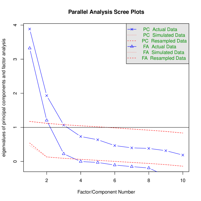
Figure 8: Screeplot for factor number of Sample B

Because of the factor correlations we chose an oblique transformation, namely Oblimin, for the exploratory factor analyses. We display the loadings for Samples A and B in Table 25.

Table 25: Factor loadings of Oblimin-transformed Polychoric EFA on Samples A and B

	Factors			Uniqueness
	Collection	Awareness	Control
ctrl1			0.75	0.43
ctrl2		0.29	0.59	0.39
ctrl3		0.46		0.58
awa1		0.75		0.39
awa2		0.66		0.45
awa3	0.26		0.56	0.62
coll1	0.86			0.33
coll2	0.69			0.45
coll3	0.79			0.30
coll4	0.59			0.47
SS loadings	2.26	1.39	1.30
Proportion Var	0.23	0.14	0.13
Cumulative Var	0.23	0.37	0.50
Note: $\chi^{2}(18)=19.515,p=.361$, Variance explained $R^{2}=.50$

(a) EFA on Sample A ($N_{\mathsf{A}}=204$)

	Factors			Uniqueness
	Collection	Awareness	Control
ctrl1			0.66	0.48
ctrl2			0.89	0.25
ctrl3	0.29		0.29	0.65
awa1		0.95		0.17
awa2		0.76		0.29
awa3	0.38	0.32		0.61
coll1	0.84			0.35
coll2	0.78			0.37
coll3	0.93			0.15
coll4	0.84			0.25
SS loadings	3.11	1.63	1.35
Proportion Var	0.31	0.16	0.14
Cumulative Var	0.31	0.47	0.61
Note: $\chi^{2}(18)=24.971,p=.126$, Variance explained $R^{2}=.61$

(b) EFA on Sample B ($N_{\mathsf{B}}=371$)

In Figure 9 we display the biplot of the exploratory factor analysis on Sample B. Therein, one can clearly see the misloading of ctrl3 and awa3.

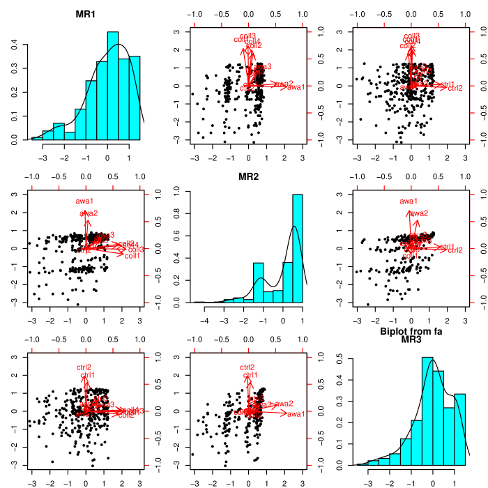
Figure 9: Biplot of the EFA of sample B

CFA of IUIPC-10

We display the overview of the different estimations of IUIPC-10 on Sample B in Table 26. It includes the factor loadings as well as scaled and unscaled fit statistics.

Table 26: Overview of IUIPC-10 CFAs with different estimators on Sample B

ML MLM WLSMVS Estimate $\mathit{SE}$ $z$ $p$ Estimate $\mathit{SE}$ $z$ $p$ Estimate $\mathit{SE}$ $z$ $p$ Factor Loadings ctrl ctrl1 1.00⁺ 1.00⁺ 1.00⁺ ctrl2 1.00 0.12 8.50 $<.001$ 1.00 0.11 8.76 $<.001$ 1.00 0.09 11.50 $<.001$ ctrl3 0.59 0.09 6.33 $<.001$ 0.59 0.11 5.36 $<.001$ 0.95 0.08 11.59 $<.001$ aware awa1 1.00⁺ 1.00⁺ 1.00⁺ awa2 1.13 0.11 10.26 $<.001$ 1.13 0.13 8.53 $<.001$ 1.07 0.10 11.08 $<.001$ awa3 0.90 0.12 7.39 $<.001$ 0.90 0.14 6.64 $<.001$ 0.92 0.08 11.55 $<.001$ collect coll1 1.00⁺ 1.00⁺ 1.00⁺ coll2 0.76 0.05 16.50 $<.001$ 0.76 0.05 14.86 $<.001$ 0.96 0.03 37.00 $<.001$ coll3 1.06 0.05 21.75 $<.001$ 1.06 0.04 23.63 $<.001$ 1.14 0.02 47.74 $<.001$ coll4 0.95 0.05 19.64 $<.001$ 0.95 0.05 18.14 $<.001$ 1.06 0.02 43.02 $<.001$ iuipc collect 0.41 0.08 5.14 $<.001$ 0.41 0.08 5.42 $<.001$ 0.46 0.04 10.78 $<.001$ ctrl 0.42 0.07 5.88 $<.001$ 0.42 0.07 6.05 $<.001$ 0.52 0.05 10.35 $<.001$ aware 0.36 0.06 6.54 $<.001$ 0.36 0.06 6.40 $<.001$ 0.73 0.07 10.39 $<.001$ Intercepts ctrl1 5.97 0.05 123.59 $<.001$ 5.97 0.05 123.59 $<.001$ 0.00⁺ ctrl2 5.96 0.05 122.96 $<.001$ 5.96 0.05 122.96 $<.001$ 0.00⁺ ctrl3 5.96 0.05 115.20 $<.001$ 5.96 0.05 115.20 $<.001$ 0.00⁺ awa1 6.68 0.03 234.36 $<.001$ 6.68 0.03 234.36 $<.001$ 0.00⁺ awa2 6.62 0.03 226.48 $<.001$ 6.62 0.03 226.48 $<.001$ 0.00⁺ awa3 6.25 0.04 146.99 $<.001$ 6.25 0.04 146.99 $<.001$ 0.00⁺ coll1 5.26 0.07 74.70 $<.001$ 5.26 0.07 74.70 $<.001$ 0.00⁺ coll2 5.76 0.06 100.28 $<.001$ 5.76 0.06 100.28 $<.001$ 0.00⁺ coll3 5.69 0.06 88.30 $<.001$ 5.69 0.06 88.30 $<.001$ 0.00⁺ coll4 5.73 0.06 90.65 $<.001$ 5.73 0.06 90.65 $<.001$ 0.00⁺ Fit Indices $\chi^{2}(\mathit{df})$ 163.69 (32) $<.001$ 163.69 $<.001$ 213.83 $<.001$ CFI .92 .92 .98 GFI 1.00 1.00 .99 RMSEA .11 $[.09,.12]$ $<.001$ .11 $[.09,.12]$ $<.001$ .12 $[.11,.14]$ $<.001$ SRMR .10 .10 .10 Scaled $\chi^{2}(\mathit{df})$ 131.42 (32) $<.001$ 181.15 (14.95) $<.001$ CAIC 294.264 294.264 447.278 Scaled CAIC 261.990 414.598

Note: $N_{\mathsf{B}}^{\prime}=371$; ⁺Fixed parameter; the ML CFA model without outlier correction with $N_{\mathsf{B}}=380$ yielded $\chi^{2}(32)=202.789,p<.001$; $\mathsf{CFI}=.90$; $\mathsf{GFI}=1.00$; $\mathsf{RMSEA}=.12[.10,.14]$; $\mathsf{SRMR}=.11$; $\mathsf{CAIC}=333.758$.

In the following we also offer the residuals, that is, correlation and (standardized, if possible) covariance residuals for all CFAs computed. Table 27 includes the residuals of the replication of the approach of Malhotra et al. [45], that is, computing an ML-estimated CFA on ordinal, non-normal data without outlier treatment.

Table 28 contains the residuals of the ML-estimation on our outlier-treated Sample B, corresponding to the left column on Table 26. We can see that as a tendency the residuals of the replication in Table 27 and the outlier-treated ML-estimation in Table 28 are largely aligned.

able 29 displays the residuals of the MLM estimation on Sample B, which is the touch stone of the paper (center column of Table 26.

Finally, Table 30 shows the residuals of the WLSMVS estimation of IUIPC-10. Note that lavaan cannot compute standardized covariance residuals for a WLSMVS estimation and that we have included the raw covariance residuals instead.

Table 27: Residuals of the ML-estimated CFA of IUIPC-10 on Sample B (as done in IUIPC itself, without outlier treatment)

	1	2	3	4	5	6	7	8	9	10
1. ctrl1	—
2. ctrl2	0.013	—
3. ctrl3	-0.037	-0.023	—
4. awa1	-0.047	-0.039	0.155	—
5. awa2	-0.023	-0.003	0.179	0.013	—
6. awa3	0.08	0.031	0.185	-0.009	-0.047	—
7. coll1	-0.089	-0.087	0.211	-0.136	-0.099	0.226	—
8. coll2	-0.024	-0.041	0.249	0.062	0.067	0.182	0.034	—
9. coll3	0.011	-0.049	0.25	-0.083	-0.042	0.284	-0.003	0.001	—
10. coll4	0.054	-0.007	0.26	0.061	0.029	0.374	-0.001	-0.033	0.005	—
Note: Correlation residuals in absolute $>0.1$ are marked

(a) Correlation residuals

	1	2	3	4	5	6	7	8	9	10
1. ctrl1	—
2. ctrl2	5.149	—
3. ctrl3	-2.21	-1.819	—
4. awa1	-2.021	-1.8	3.474	—
5. awa2	-1.082	-0.155	4.071	5.177	—
6. awa3	1.842	0.73	3.911	-0.586	-3.71	—
7. coll1	-2.632	-2.857	4.217	-4.399	-3.388	4.608	—
8. coll2	-0.645	-1.17	4.992	1.744	1.927	3.919	2.065	—
9. coll3	0.402	-2.202	5.12	-3.665	-2.086	5.905	-0.801	0.078	—
10. coll4	1.754	-0.26	5.344	2.237	1.093	7.846	-0.132	-2.91	1.505	—
Note: Statistically significant residuals ($\mathsf{abs}>1.96$) are marked

(b) Standardized residuals

Table 28: Residuals of the ML-estimated CFA of IUIPC-10 on Sample B (with outlier treatment)

	1	2	3	4	5	6	7	8	9	10
1. ctrl1	—
2. ctrl2	0.021	—
3. ctrl3	-0.046	-0.022	—
4. awa1	-0.042	-0.062	0.089	—
5. awa2	-0.01	0	0.115	0.018	—
6. awa3	0.048	0.015	0.163	-0.007	-0.049	—
7. coll1	-0.082	-0.085	0.189	-0.147	-0.111	0.206	—
8. coll2	-0.025	-0.068	0.211	0.034	0.032	0.186	0.037	—
9. coll3	0.001	-0.069	0.234	-0.065	-0.031	0.264	-0.007	0.003	—
10. coll4	0.051	-0.043	0.231	0.024	0.003	0.345	0.006	-0.038	0.004	—
Note: Correlation residuals in absolute $>0.1$ are marked

(a) Correlation residuals

	1	2	3	4	5	6	7	8	9	10
1. ctrl1	—
2. ctrl2	4.214	—
3. ctrl3	-2.68	-1.249	—
4. awa1	-1.676	-2.408	2.097	—
5. awa2	-0.484	0.003	2.853	4.646	—
6. awa3	1.157	0.352	3.514	-0.367	-4.015	—
7. coll1	-2.4	-2.494	3.852	-4.349	-3.684	4.255	—
8. coll2	-0.695	-1.864	4.314	0.955	0.957	4.03	2.194	—
9. coll3	0.028	-2.708	4.91	-2.643	-1.654	5.684	-1.731	0.495	—
10. coll4	1.667	-1.386	4.848	0.818	0.111	7.349	0.611	-3.36	1.482	—
Note: Statistically significant residuals ($\mathsf{abs}>1.96$) are marked

(b) Standardized residuals

Table 29: Residuals of the MLM-estimated CFA of IUIPC-10 on Sample BCaptionExplanations.
The highlighted distinctive residual patterns show a poor local fit. They indicate misloadings of ctrl3 and awa3.

	1	2	3	4	5	6	7	8	9	10
1. ctrl1	—
2. ctrl2	0.021	—
3. ctrl3	-0.046	-0.022	—
4. awa1	-0.042	-0.062	0.089	—
5. awa2	-0.01	0	0.115	0.018	—
6. awa3	0.048	0.015	0.163	-0.007	-0.049	—
7. coll1	-0.082	-0.085	0.189	-0.147	-0.111	0.206	—
8. coll2	-0.025	-0.068	0.211	0.034	0.032	0.186	0.037	—
9. coll3	0.001	-0.069	0.234	-0.065	-0.031	0.264	-0.007	0.003	—
10. coll4	0.051	-0.043	0.231	0.024	0.003	0.345	0.006	-0.038	0.004	—
Note: Correlation residuals in absolute $>0.1$ are marked

(a) Correlation residuals

	1	2	3	4	5	6	7	8	9	10
1. ctrl1	—
2. ctrl2	3.703	—
3. ctrl3	-2.345	-1.016	—
4. awa1	-1.585	-2.466	1.921	—
5. awa2	-0.457	0.003	2.597	4.618	—
6. awa3	0.972	0.379	3.012	-0.36	-3.891	—
7. coll1	-2.304	-2.617	3.324	-4.525	-3.544	3.878	—
8. coll2	-0.669	-1.843	4.334	0.706	0.845	3.971	2.035	—
9. coll3	0.031	-2.609	4.142	-2.448	-1.365	5.144	-1.384	0.405	—
10. coll4	1.293	-1.429	4.284	0.688	0.101	5.912	0.475	-2.636	1.397	—
Note: Statistically significant residuals ($\mathsf{abs}>1.96$) are marked

(b) Standardized residuals

Table 30: Residuals of the WLSMVS-estimated CFA of IUIPC-10 on Sample B

	1	2	3	4	5	6	7	8	9	10
1. ctrl1	—
2. ctrl2	0.123	—
3. ctrl3	-0.151	-0.111	—
4. awa1	-0.003	-0.017	0.015	—
5. awa2	0.043	0.052	0.03	0.09	—
6. awa3	-0.054	-0.075	0.008	-0.151	-0.223	—
7. coll1	-0.151	-0.163	0.082	-0.248	-0.214	0.079	—
8. coll2	-0.084	-0.129	0.151	-0.041	-0.032	0.078	0.039	—
9. coll3	-0.053	-0.118	0.133	-0.152	-0.111	0.129	-0.003	0.005	—
10. coll4	-0.007	-0.088	0.138	-0.049	-0.076	0.221	0.008	-0.043	0	—
Note: Correlation residuals in absolute $>0.1$ are marked

(a) Correlation residuals

	1	2	3	4	5	6	7	8	9	10
1. ctrl1	—
2. ctrl2	0.123	—
3. ctrl3	-0.151	-0.111	—
4. awa1	-0.003	-0.017	0.015	—
5. awa2	0.043	0.052	0.03	0.09	—
6. awa3	-0.054	-0.075	0.008	-0.151	-0.223	—
7. coll1	-0.151	-0.163	0.082	-0.248	-0.214	0.079	—
8. coll2	-0.084	-0.129	0.151	-0.041	-0.032	0.078	0.039	—
9. coll3	-0.053	-0.118	0.133	-0.152	-0.111	0.129	-0.003	0.005	—
10. coll4	-0.007	-0.088	0.138	-0.049	-0.076	0.221	0.008	-0.043	0	—
Note: Standardized residuals are not available for estimator WLSMVS

(b) Covariance residuals

Respecification: IUIPC-8

We computed the models for the respecification IUIPC-8 on Sample B.

Again, we include the residuals for the corresponding models. Table 31 displays the residuals for the ML estimation on IUIPC-8. Already in this estimation, we observe a far lower number of statistically significant covariance residuals than in the IUIPC-10 model.

The MLM estimation with robust standard errors is shown in Table 32. Here we have two statistically significant residuals with concerning correlations left. We inspected the questionnaire itself for evidence of method correlation. We found specifically that coll1 and coll3 follow a parallel construction with the stem “It bothers me…,” which could lead to correlated error variances on substantive grounds. Testing the this variant with an LRT difference test on nested models, we found that the difference is statistically significant in the ML estimation, but not under Satorra-Bentler correction, $\chi^{2}(1)=3.975,p=.046$ and $\chi^{2}(1)=2.548,p=.110$, respectively. The difference between the variants is even less pronounced under WLSMVS estimation. Hence, we choose to keep the model without correlated errors.

Table 33, then, shows the residuals for the WLSMVS estimated model on Sample B. We observe that the WLSMVS estimation offers a perfect fit, passing even the exact-fit hypothesis at a sample size of $N^{\prime}_{\mathsf{B}}=391$.

Figure 10: CFA paths plot with standardized estimates of the respecified IUIPC-8 on Sample B. Note: The coefficients are standardized

Table 31: Residuals of the ML CFA of IUIPC-8 on Sample B

	1	2	3	4	5	6	7	8
1. ctrl1	—
2. ctrl2	0	—
3. awa1	0.004	-0.011	—
4. awa2	-0.007	0.01	0	—
5. coll1	-0.052	-0.053	-0.099	-0.086	—
6. coll2	0.003	-0.038	0.08	0.056	0.037	—
7. coll3	0.035	-0.032	-0.009	-0.002	-0.008	0.002	—
8. coll4	0.083	-0.009	0.076	0.03	0.007	-0.037	0.005	—
Note: Correlation residuals in absolute $>0.1$ are marked

(a) Correlation residuals

	1	2	3	4	5	6	7	8
1. ctrl1	—
2. ctrl2	0	—
3. awa1	0.2	-0.494	—
4. awa2	-1.067	1.292	0	—
5. coll1	-1.555	-1.529	-2.647	-3.1	—
6. coll2	0.084	-1.033	2.073	1.739	2.192	—
7. coll3	1.458	-1.215	-0.288	-0.175	-2.067	0.432	—
8. coll4	2.747	-0.284	2.283	1.227	0.668	-3.231	1.683	—
Note: Statistically significant residuals ($\mathsf{abs}>1.96$) are marked

(b) Standardized residuals

Table 32: Residuals of the MLM CFA of IUIPC-8 on Sample B

	1	2	3	4	5	6	7	8
1. ctrl1	—
2. ctrl2	0	—
3. awa1	0.004	-0.011	—
4. awa2	-0.007	0.01	0	—
5. coll1	-0.052	-0.053	-0.099	-0.086	—
6. coll2	0.003	-0.038	0.08	0.056	0.037	—
7. coll3	0.035	-0.032	-0.009	-0.002	-0.008	0.002	—
8. coll4	0.083	-0.009	0.076	0.03	0.007	-0.037	0.005	—
Note: Correlation residuals in absolute $>0.1$ are marked

(a) Correlation residuals

	1	2	3	4	5	6	7	8
1. ctrl1	—
2. ctrl2	0	—
3. awa1	0.191	-0.501	—
4. awa2	-0.976	1.345	0	—
5. coll1	-1.482	-1.668	-2.724	-3.134	—
6. coll2	0.082	-1.066	1.584	1.476	2.033	—
7. coll3	1.589	-1.245	-0.254	-0.155	-1.653	0.349	—
8. coll4	2.133	-0.299	1.961	1.17	0.524	-2.531	1.58	—
Note: Statistically significant residuals ($\mathsf{abs}>1.96$) are marked

(b) Standardized residuals

Table 33: Residuals of the WLSMVS CFA of IUIPC-8 on Sample B

	1	2	3	4	5	6	7	8
1. ctrl1	—
2. ctrl2	0	—
3. awa1	-0.017	0.003	—
4. awa2	-0.017	0.032	0	—
5. coll1	-0.071	-0.068	-0.132	-0.115	—
6. coll2	-0.005	-0.037	0.071	0.065	0.034	—
7. coll3	0.04	-0.009	-0.019	0.003	-0.012	0.003	—
8. coll4	0.082	0.015	0.078	0.034	0.008	-0.036	0.004	—
Note: Correlation residuals in absolute $>0.1$ are marked

(a) Correlation residuals

	1	2	3	4	5	6	7	8
1. ctrl1	—
2. ctrl2	0	—
3. awa1	-0.017	0.003	—
4. awa2	-0.017	0.032	0	—
5. coll1	-0.071	-0.068	-0.132	-0.115	—
6. coll2	-0.005	-0.037	0.071	0.065	0.034	—
7. coll3	0.04	-0.009	-0.019	0.003	-0.012	0.003	—
8. coll4	0.082	0.015	0.078	0.034	0.008	-0.036	0.004	—
Note: Standardized residuals are not available for estimator WLSMVS

(b) Covariance residuals

Table 34: Evidence for discriminant validity of IUIPC-8 (Fornell-Larcker Criterion and Heterotrait-Monotrait Ratio) on Sample B

	1	2	3	4
1. ctrl	0.747
2. aware	0.477	0.803
3. collect	0.171	0.265	0.848
4. iuipc	0.556	0.859	0.308	0.825
Note: The diagonal contains the $\sqrt{\mathit{AVE}}$

(a) Fornell-Larcker

	1	2	3
1. ctrl	—
2. aware	0.48	—
3. collect	0.16	0.28	—

(b) HTMT Ratio

Validation

The validation CFAs were computed on Sample V.

IUIPC-10 Validation

First, we consider the performance of IUIPC-10 on this independent sample.

We also provide the comparison with the standardized solution for the MLM estimation in Table 35. Again, we observe that the variance explained by the indicators ctrl3 and awa3 is intolerably low, with $R^{2}=.22$ and $R^{2}=.15$ respectively. Hence, the validation CFA of IUIPC-10 indicates the same convergent validity problem seen in the main analysis on base Sample B.

Table 35: Factor loadings and their standardized solution of the MLM CFA of IUIPC-10 on validation Sample V

Factor	Indicator	Factor Loading				Standardized Solution				Reliability
		$\lambda$	$\mathit{SE}_{\lambda}$	$Z_{\lambda}$	$p_{\lambda}$	$\beta$	$\mathit{SE}_{\beta}$	$Z_{\beta}$	$p_{\beta}$	$R^{2}$	$\mathit{AVE}$	$\alpha$	$\omega$	$\mathit{S/\!N}_{\omega}$
ctrl	ctrl1	$1.00^{+}$				0.68	0.06	11.19	$<.001$	0.46	0.41	0.64	0.67	2.00
	ctrl2	$1.08\phantom{{}^{+}}$	0.12	8.91	$<.001$	0.75	0.05	14.79	$<.001$	0.56
	ctrl3	$0.71\phantom{{}^{+}}$	0.09	7.47	$<.001$	0.47	0.05	9.90	$<.001$	0.22
aware	awa1	$1.00^{+}$				0.70	0.05	15.13	$<.001$	0.49	0.33	0.56	0.59	1.45
	awa2	$0.97\phantom{{}^{+}}$	0.10	9.58	$<.001$	0.75	0.05	13.73	$<.001$	0.57
	awa3	$0.79\phantom{{}^{+}}$	0.13	6.25	$<.001$	0.39	0.05	7.34	$<.001$	0.15
collect	coll1	$1.00^{+}$				0.76	0.03	25.47	$<.001$	0.58	0.63	0.86	0.87	6.55
	coll2	$0.62\phantom{{}^{+}}$	0.06	11.00	$<.001$	0.64	0.05	13.07	$<.001$	0.41
	coll3	$1.04\phantom{{}^{+}}$	0.06	17.97	$<.001$	0.92	0.02	51.13	$<.001$	0.85
	coll4	$0.89\phantom{{}^{+}}$	0.05	16.70	$<.001$	0.80	0.03	30.70	$<.001$	0.64
iuipc	collect	$0.45\phantom{{}^{+}}$	0.07	6.42	$<.001$	0.43	0.06	6.81	$<.001$	0.18
	ctrl	$0.46\phantom{{}^{+}}$	0.06	7.69	$<.001$	0.67	0.07	9.61	$<.001$	0.45
	aware	$0.45\phantom{{}^{+}}$	0.06	7.97	$<.001$	0.93	0.10	9.40	$<.001$	0.87
Note: + fixed parameter; the standardized solution is STDALL

Considering the residuals on Sample V, we find the same pattern as in the main analysis in the Tables 36 (ML estimation) and 37 (MLM estimation). The WLSMVS estimation in Table 38 yield related correlation patterns, perhaps not quite as pronounced.

Table 36: Residuals of the ML validation CFA of IUIPC-10 on Sample V

	1	2	3	4	5	6	7	8	9	10
1. ctrl1	—
2. ctrl2	0.03	—
3. ctrl3	-0.029	-0.041	—
4. awa1	-0.018	0.013	0.115	—
5. awa2	-0.046	-0.041	0.071	0.023	—
6. awa3	-0.01	0.051	0.062	-0.062	-0.019	—
7. coll1	-0.082	-0.036	0.153	-0.092	-0.015	0.177	—
8. coll2	0.053	0.082	0.187	-0.051	0.026	0.267	0.036	—
9. coll3	-0.034	-0.054	0.173	-0.075	-0.013	0.196	0.001	-0.009	—
10. coll4	-0.079	-0.021	0.199	0.003	0.018	0.17	-0.017	-0.016	0.006	—
Note: Correlation residuals in absolute $>0.1$ are marked

(a) Correlation residuals

	1	2	3	4	5	6	7	8	9	10
1. ctrl1	—
2. ctrl2	4.171	—
3. ctrl3	-1.483	-2.89	—
4. awa1	-0.699	0.582	3.193	—
5. awa2	-2.001	-2.142	1.991	3.945	—
6. awa3	-0.264	1.344	1.492	-2.926	-1.091	—
7. coll1	-2.308	-1.122	3.492	-2.778	-0.488	4.002	—
8. coll2	1.326	2.154	4.256	-1.369	0.727	5.944	1.697	—
9. coll3	-1.282	-2.428	4.139	-3.224	-0.67	4.605	0.36	-1.352	—
10. coll4	-2.347	-0.701	4.589	0.108	0.613	3.971	-1.424	-0.908	1.68	—
Note: Statistically significant residuals ($\mathsf{abs}>1.96$) are marked

(b) Standardized residuals

Table 37: Residuals of the MLM validation CFA of IUIPC-10 on Sample V

	1	2	3	4	5	6	7	8	9	10
1. ctrl1	—
2. ctrl2	0.03	—
3. ctrl3	-0.029	-0.041	—
4. awa1	-0.018	0.013	0.115	—
5. awa2	-0.046	-0.041	0.071	0.023	—
6. awa3	-0.01	0.051	0.062	-0.062	-0.019	—
7. coll1	-0.082	-0.036	0.153	-0.092	-0.015	0.177	—
8. coll2	0.053	0.082	0.187	-0.051	0.026	0.267	0.036	—
9. coll3	-0.034	-0.054	0.173	-0.075	-0.013	0.196	0.001	-0.009	—
10. coll4	-0.079	-0.021	0.199	0.003	0.018	0.17	-0.017	-0.016	0.006	—
Note: Correlation residuals in absolute $>0.1$ are marked

(a) Correlation residuals

	1	2	3	4	5	6	7	8	9	10
1. ctrl1	—
2. ctrl2	3.976	—
3. ctrl3	-1.571	-3.442	—
4. awa1	-0.69	0.514	3.117	—
5. awa2	-1.906	-1.868	1.868	3.585	—
6. awa3	-0.262	0.925	1.449	-2.712	-1.069	—
7. coll1	-2.166	-0.842	3.426	-2.297	-0.467	2.963	—
8. coll2	1.315	1.432	4.211	-1.117	0.704	3.325	0.976	—
9. coll3	-1.217	-2.179	4.163	-2.835	-0.574	3.148	0.24	-0.839	—
10. coll4	-2.303	-0.633	4.52	0.089	0.62	2.992	-0.901	-0.624	0.956	—
Note: Statistically significant residuals ($\mathsf{abs}>1.96$) are marked

(b) Standardized residuals

Table 38: Residuals of the WLSMVS validation CFA of IUIPC-10 on Sample V

	1	2	3	4	5	6	7	8	9	10
1. ctrl1	—
2. ctrl2	0.066	—
3. ctrl3	-0.108	-0.155	—
4. awa1	0.024	0.023	0.086	—
5. awa2	-0.021	-0.022	0.021	0.055	—
6. awa3	-0.067	-0.027	-0.028	-0.104	-0.068	—
7. coll1	-0.137	-0.105	0.092	-0.123	-0.06	0.098	—
8. coll2	0.02	0.021	0.142	-0.092	-0.001	0.178	0.017	—
9. coll3	-0.082	-0.104	0.097	-0.097	-0.068	0.103	0.011	-0.024	—
10. coll4	-0.116	-0.062	0.139	-0.02	-0.019	0.084	-0.012	-0.023	0.01	—
Note: Correlation residuals in absolute $>0.1$ are marked

(a) Correlation residuals

	1	2	3	4	5	6	7	8	9	10
1. ctrl1	—
2. ctrl2	0.066	—
3. ctrl3	-0.108	-0.155	—
4. awa1	0.024	0.023	0.086	—
5. awa2	-0.021	-0.022	0.021	0.055	—
6. awa3	-0.067	-0.027	-0.028	-0.104	-0.068	—
7. coll1	-0.137	-0.105	0.092	-0.123	-0.06	0.098	—
8. coll2	0.02	0.021	0.142	-0.092	-0.001	0.178	0.017	—
9. coll3	-0.082	-0.104	0.097	-0.097	-0.068	0.103	0.011	-0.024	—
10. coll4	-0.116	-0.062	0.139	-0.02	-0.019	0.084	-0.012	-0.023	0.01	—
Note: Standardized residuals are not available for estimator WLSMVS

(b) Covariance residuals

Table 39: Evidence for discriminant validity of IUIPC-10 (Fornell-Larcker Criterion and Heterotrait-Monotrait Ratio) on Sample V

	1	2	3	4
1. ctrl	0.638
2. aware	0.625	0.572
3. collect	0.285	0.399	0.793
4. iuipc	0.668	0.935	0.427	0.717
Note: The diagonal contains the $\sqrt{\mathit{AVE}}$

(a) Fornell-Larcker

	1	2	3
1. ctrl	—
2. aware	0.73	—
3. collect	0.39	0.53	—

(b) HTMT Ratio

IUIPC-8 Validation

Considering the standardized loadings in Table 40, we find that the indicator variables explain more consistently more than $50\%$ of the variance. Indicator coll2 is an exception to note.

Table 40: Factor loadings and their standardized solution of the MLM CFA of IUIPC-8 on validation Sample V

Factor	Indicator	Factor Loading				Standardized Solution				Reliability
		$\lambda$	$\mathit{SE}_{\lambda}$	$Z_{\lambda}$	$p_{\lambda}$	$\beta$	$\mathit{SE}_{\beta}$	$Z_{\beta}$	$p_{\beta}$	$R^{2}$	$\mathit{AVE}$	$\alpha$	$\omega$	$\mathit{S/\!N}_{\omega}$
ctrl	ctrl1	$1.00^{+}$				0.67	0.06	10.51	$<.001$	0.45	0.54	0.70	0.70	2.33
	ctrl2	$1.16\phantom{{}^{+}}$	0.16	7.18	$<.001$	0.79	0.06	12.49	$<.001$	0.63
aware	awa1	$1.00^{+}$				0.72	0.04	16.16	$<.001$	0.52	0.55	0.71	0.71	2.41
	awa2	$0.95\phantom{{}^{+}}$	0.11	8.68	$<.001$	0.76	0.06	12.93	$<.001$	0.58
collect	coll1	$1.00^{+}$				0.76	0.03	25.41	$<.001$	0.58	0.63	0.86	0.87	6.54
	coll2	$0.62\phantom{{}^{+}}$	0.06	10.96	$<.001$	0.64	0.05	12.93	$<.001$	0.40
	coll3	$1.04\phantom{{}^{+}}$	0.06	17.98	$<.001$	0.93	0.02	50.74	$<.001$	0.86
	coll4	$0.89\phantom{{}^{+}}$	0.05	16.62	$<.001$	0.80	0.03	30.48	$<.001$	0.64
iuipc	collect	$0.39\phantom{{}^{+}}$	0.07	5.25	$<.001$	0.37	0.07	5.39	$<.001$	0.14
	ctrl	$0.40\phantom{{}^{+}}$	0.07	5.74	$<.001$	0.59	0.09	6.90	$<.001$	0.35
	aware	$0.46\phantom{{}^{+}}$	0.07	6.45	$<.001$	0.93	0.13	7.43	$<.001$	0.87
Note: + fixed parameter; the standardized solution is STDALL

The residuals displayed in Tables 41 (ML estimation), 42 (MLM estimation), and 43 are all in good shape, indicating a good local fit throughout.

Table 41: Residuals of the ML validation CFA of IUIPC-8 on Sample V

	1	2	3	4	5	6	7	8
1. ctrl1	—
2. ctrl2	0	—
3. awa1	0.012	0.026	—
4. awa2	-0.009	-0.022	0	—
5. coll1	-0.046	-0.006	-0.068	0.014	—
6. coll2	0.082	0.108	-0.031	0.051	0.037	—
7. coll3	0.009	-0.017	-0.047	0.022	0.001	-0.008	—
8. coll4	-0.042	0.011	0.028	0.048	-0.016	-0.014	0.005	—
Note: Correlation residuals in absolute $>0.1$ are marked

(a) Correlation residuals

	1	2	3	4	5	6	7	8
1. ctrl1	—
2. ctrl2	0	—
3. awa1	0.635	1.745	—
4. awa2	-0.576	-1.817	0	—
5. coll1	-1.277	-0.19	-2.084	0.462	—
6. coll2	2.039	2.871	-0.834	1.415	1.762	—
7. coll3	0.302	-0.907	-2.085	1.13	0.194	-1.251	—
8. coll4	-1.216	0.37	0.912	1.654	-1.398	-0.804	1.609	—
Note: Statistically significant residuals ($\mathsf{abs}>1.96$) are marked

(b) Standardized residuals

Table 42: Residuals of the MLM validation CFA of IUIPC-8 on Sample V

	1	2	3	4	5	6	7	8
1. ctrl1	—
2. ctrl2	0	—
3. awa1	0.012	0.026	—
4. awa2	-0.009	-0.022	0	—
5. coll1	-0.046	-0.006	-0.068	0.014	—
6. coll2	0.082	0.108	-0.031	0.051	0.037	—
7. coll3	0.009	-0.017	-0.047	0.022	0.001	-0.008	—
8. coll4	-0.042	0.011	0.028	0.048	-0.016	-0.014	0.005	—
Note: Correlation residuals in absolute $>0.1$ are marked

(a) Correlation residuals

	1	2	3	4	5	6	7	8
1. ctrl1	—
2. ctrl2	0	—
3. awa1	0.579	1.623	—
4. awa2	-0.524	-1.648	0	—
5. coll1	-1.196	-0.138	-1.719	0.441	—
6. coll2	2.041	1.895	-0.681	1.371	1.003	—
7. coll3	0.287	-0.775	-1.761	0.94	0.129	-0.778	—
8. coll4	-1.179	0.332	0.745	1.634	-0.887	-0.552	0.928	—
Note: Statistically significant residuals ($\mathsf{abs}>1.96$) are marked

(b) Standardized residuals

Table 43: Residuals of the WLSMVS validation CFA of IUIPC-8 on Sample V

	1	2	3	4	5	6	7	8
1. ctrl1	—
2. ctrl2	0	—
3. awa1	0.036	0.026	—
4. awa2	-0.015	-0.027	0	—
5. coll1	-0.069	-0.035	-0.064	-0.001	—
6. coll2	0.083	0.086	-0.036	0.057	0.023	—
7. coll3	-0.002	-0.021	-0.029	0.002	0.005	-0.019	—
8. coll4	-0.045	0.012	0.043	0.045	-0.012	-0.014	0.007	—
Note: Correlation residuals in absolute $>0.1$ are marked

(a) Correlation residuals

	1	2	3	4	5	6	7	8
1. ctrl1	—
2. ctrl2	0	—
3. awa1	0.036	0.026	—
4. awa2	-0.015	-0.027	0	—
5. coll1	-0.069	-0.035	-0.064	-0.001	—
6. coll2	0.083	0.086	-0.036	0.057	0.023	—
7. coll3	-0.002	-0.021	-0.029	0.002	0.005	-0.019	—
8. coll4	-0.045	0.012	0.043	0.045	-0.012	-0.014	0.007	—
Note: Standardized residuals are not available for estimator WLSMVS

(b) Covariance residuals

Table 44: Evidence for discriminant validity of IUIPC-8 (Fornell-Larcker Criterion and Heterotrait-Monotrait Ratio) on Sample V

	1	2	3	4
1. ctrl	0.735
2. aware	0.547	0.74
3. collect	0.218	0.344	0.793
4. iuipc	0.588	0.93	0.37	0.774
Note: The diagonal contains the $\sqrt{\mathit{AVE}}$

(a) Fornell-Larcker

	1	2	3
1. ctrl	—
2. aware	0.55	—
3. collect	0.24	0.35	—

(b) HTMT Ratio

Used Software

The statistics were computed in R (v. 3.6.2) using the package lavaan (v. 0.6-5) for the confirmatory factor analyses. We included a truncated version of the R sessionInfo() below, including the attached packages and their version numbers.

R version 3.6.2 (2019-12-12)
Platform: x86_64-apple-darwin15.6.0 (64-bit)
Running under: macOS High Sierra 10.13.6

Matrix products: default

Random number generation:
 RNG:     L’Ecuyer-CMRG
 Normal:  Inversion
 Sample:  Rejection

locale:
 en_GB.UTF-8

attached base packages:
 stats     graphics  grDevices utils     datasets  methods   base

other attached packages:
 semTable_1.7          semPower_1.0.0        pastecs_1.3.21        matrixcalc_1.0-3
 GPArotation_2014.11-1 semTools_0.5-2        semPlot_1.1.2         lavaan_0.6-5
 dplyr_0.8.4           weights_1.0.1         mice_3.7.0            gdata_2.18.0
 Hmisc_4.3-1           ggplot2_3.2.1         Formula_1.2-3         survival_3.1-8
 lattice_0.20-38       xtable_1.8-4          psych_1.9.12.31

References

- [1] M. Ab Hamid, W. Sami, and M. Sidek. Discriminant validity assessment: Use of Fornell & Larcker criterion versus HTMT criterion. In Journal of Physics: Conference Series, volume 890, page 012163. IOP Publishing, 2017.
- [2] J. C. Anderson and D. W. Gerbing. Structural equation modeling in practice: A review and recommended two-step approach. Psychological bulletin, 103(3):411, 1988.
- [3] J. C. Anderson, D. W. Gerbing, and J. E. Hunter. On the assessment of unidimensional measurement: Internal and external consistency, and overall consistency criteria. Journal of marketing research, 24(4):432–437, 1987.
- [4] N. M. Barbosa, J. S. Park, Y. Yao, and Y. Wang. “what if?” predicting individual users’ smart home privacy preferences and their changes. Proceedings on Privacy Enhancing Technologies, 2019(4):211–231, 2019.
- [5] Z. Benenson, A. Girard, and I. Krontiris. User acceptance factors for anonymous credentials: An empirical investigation. In WEIS, 2015.
- [6] K. A. Bollen. Structural equations with latent variables, chapter Measurement models: The relation between latent and observed variables, pages 179–225. Wiley Online Library, 1989.
- [7] D. Borsboom, G. J. Mellenbergh, and J. Van Heerden. The concept of validity. Psychological review, 111(4):1061, 2004.
- [8] J. A. Bovaird and N. A. Koziol. Measurement models for ordered-categorical indicators. In R. H. Hoyle, editor, Handbook of Structural Equation Modeling, pages 495–511. The Guilford Press, 2012.
- [9] A. Braunstein, L. Granka, and J. Staddon. Indirect content privacy surveys: measuring privacy without asking about it. In Proceedings of the Seventh Symposium on Usable Privacy and Security, pages 1–14, 2011.
- [10] T. A. Brown. Confirmatory factor analysis for applied research. The Guilford Press, 2015.
- [11] M. W. Browne and R. Cudeck. Alternative ways of assessing model fit. Testing structural equation models, 154:136, 1993.
- [12] T. Buchanan, C. Paine, A. N. Joinson, and U.-D. Reips. Development of measures of online privacy concern and protection for use on the internet. Journal of the American society for information science and technology, 58(2):157–165, 2007.
- [13] J. A. Castañeda, F. J. Montoso, and T. Luque. The dimensionality of customer privacy concern on the internet. Online Information Review, 2007.
- [14] B. C. Choi and A. W. Pak. Peer reviewed: a catalog of biases in questionnaires. Preventing chronic disease, 2(1), 2005.
- [15] L. J. Cronbach and P. E. Meehl. Construct validity in psychological tests. Psychological bulletin, 52(4):281, 1955.
- [16] T. Dinev and P. Hart. Internet privacy concerns and their antecedents-measurement validity and a regression model. Behaviour & Information Technology, 23(6):413–422, 2004.
- [17] C. DiStefano. The impact of categorization with confirmatory factor analysis. Structural equation modeling, 9(3):327–346, 2002.
- [18] C. DiStefano, M. Zhu, and D. Mindrila. Understanding and using factor scores: Considerations for the applied researcher. Practical Assessment, Research, and Evaluation, 14(1):20, 2009.
- [19] T. W. Dunfee, N. C. Smith, and W. T. Ross Jr. Social contracts and marketing ethics. Journal of marketing, 63(3):14–32, 1999.
- [20] S. J. Finney and C. DiStefano. Non-normal and categorical data in structural equation modeling. Structural equation modeling: A second course, 10(6):269–314, 2006.
- [21] C. Fornell and D. F. Larcker. Evaluating structural equation models with unobservable variables and measurement error. Journal of marketing research, 18(1):39–50, 1981.
- [22] N. Gerber, P. Gerber, and M. Volkamer. Explaining the privacy paradox: A systematic review of literature investigating privacy attitude and behavior. Computers & Security, 77:226–261, 2018.
- [23] N. Gerber, B. Reinheimer, and M. Volkamer. Investigating people’s privacy risk perception. Proceedings on Privacy Enhancing Technologies, 2019(3):267–288, 2019.
- [24] D. W. Gerbing and J. C. Anderson. An updated paradigm for scale development incorporating unidimensionality and its assessment. Journal of marketing research, 25(2):186–192, 1988.
- [25] J. W. Grice. Computing and evaluating factor scores. Psychological methods, 6(4):430, 2001.
- [26] J. F. Hair, W. C. Black, B. J. Babin, and R. E. Anderson. Multivariate data analysis. Cengage Learning, 8th edition, 2019.
- [27] D. Harborth and S. Pape. German translation of the concerns for information privacy (cfip) construct. SSRN 3112207, 2018.
- [28] D. Harborth and S. Pape. Jondonym users’ information privacy concerns. In IFIP International Conference on ICT Systems Security and Privacy Protection, pages 170–184. Springer, 2018.
- [29] D. Harborth and S. Pape. How privacy concerns and trust and risk beliefs influence users’ intentions to use privacy-enhancing technologies-the case of tor. In Proceedings of the 52nd Hawaii International Conference on System Sciences, 2019.
- [30] D. Harborth, S. Pape, and K. Rannenberg. Explaining the technology use behavior of privacy-enhancing technologies: The case of tor and jondonym. Proceedings on Privacy Enhancing Technologies, 2020(2):111–128, 2020.
- [31] J. Henseler, C. M. Ringle, and M. Sarstedt. A new criterion for assessing discriminant validity in variance-based structural equation modeling. Journal of the academy of marketing science, 43(1):115–135, 2015.
- [32] L.-t. Hu and P. M. Bentler. Cutoff criteria for fit indexes in covariance structure analysis: Conventional criteria versus new alternatives. Structural equation modeling: a multidisciplinary journal, 6(1):1–55, 1999.
- [33] D. A. Kenny. Measuring model fit. http://davidakenny.net/cm/fit.htm, Nov 2015.
- [34] S. S. Kim. Data on context/reproducibility of iuipc. Personal Communication, May 2020.
- [35] R. B. Kline. Assumptions in structural equation modeling. In R. H. Hoyle, editor, Handbook of Structural Equation Modeling, pages 111–125. The Guilford Press, 2012.
- [36] R. B. Kline. Principles and practice of structural equation modeling. The Guilford Press, 4th ed. edition, 2015.
- [37] S. Kokolakis. Privacy attitudes and privacy behaviour: A review of current research on the privacy paradox phenomenon. Computers & security, 64:122–134, 2017.
- [38] C. E. Lance, M. M. Butts, and L. C. Michels. The sources of four commonly reported cutoff criteria: What did they really say? Organizational research methods, 9(2):202–220, 2006.
- [39] P. Lavrakas. Acquiescence response bias. https://methods.sagepub.com/reference/encyclopedia-of-survey-research-methods/n3.xml, 2008.
- [40] P. Lavrakas. Nondifferentiation. https://methods.sagepub.com/reference/encyclopedia-of-survey-research-methods, 2008.
- [41] P. Lavrakas. Priming. https://methods.sagepub.com/reference/encyclopedia-of-survey-research-methods, 2008.
- [42] P. Lavrakas. Social desirability. https://methods.sagepub.com/reference/encyclopedia-of-survey-research-methods, 2008.
- [43] P.-W. Lei and Q. Wu. Estimation in structural equation modeling. In R. H. Hoyle, editor, Handbook of structural equation modeling, pages 164–179. The Guilford Press, 2012.
- [44] C.-H. Li. Confirmatory factor analysis with ordinal data: Comparing robust maximum likelihood and diagonally weighted least squares. Behavior Research Methods, 48(3):936–949, 2016.
- [45] N. K. Malhotra, S. S. Kim, and J. Agarwal. Internet users’ information privacy concerns (IUIPC): The construct, the scale, and a causal model. Information systems research, 15(4):336–355, 2004.
- [46] P. S. Malone and J. B. Lubansky. Preparing data for structural equation modeling: Doing your homework. In Handbook of Structural Equation Modeling, pages 263–276. The Guilford Press, 2012.
- [47] R. P. McDonald. Structural models and the art of approximation. Perspectives on Psychological Science, 5(6):675–686, 2010.
- [48] S. Messick. Test validity and the ethics of assessment. American psychologist, 35(11):1012, 1980.
- [49] S. Messick. Validity. ETS Research Report Series, 1987(2):i–208, 1987.
- [50] A. Morton. Measuring inherent privacy concern and desire for privacy-a pilot survey study of an instrument to measure dispositional privacy concern. In 2013 International Conference on Social Computing, pages 468–477. IEEE, 2013.
- [51] B. Muthén and D. Kaplan. A comparison of some methodologies for the factor analysis of non-normal likert variables. British Journal of Mathematical and Statistical Psychology, 38(2):171–189, 1985.
- [52] A. N. Oppenheim. Questionnaire design, interviewing and attitude measurement. Continuum, 1992.
- [53] S. Preibusch. Guide to measuring privacy concern: Review of survey and observational instruments. International Journal of Human-Computer Studies, 71(12):1133–1143, 2013.
- [54] Y. Pu and J. Grossklags. Towards a model on the factors influencing social app users’ valuation of interdependent privacy. Proceedings on privacy enhancing technologies, 2016(2):61–81, 2016.
- [55] W. Revelle and D. M. Condon. Reliability. In The Wiley Handbook of Psychometric Testing: A Multidisciplinary Reference on Survey, Scale and Test Development, pages 709–749. Wiley, 1st edition, 2018.
- [56] K. S. Schwaig, A. H. Segars, V. Grover, and K. D. Fiedler. A model of consumers’ perceptions of the invasion of information privacy. Information & Management, 50(1):1–12, 2013.
- [57] S. Sharma, S. Mukherjee, A. Kumar, and W. R. Dillon. A simulation study to investigate the use of cutoff values for assessing model fit in covariance structure models. Journal of Business Research, 58(7):935–943, 2005.
- [58] J. C. Sipior, B. T. Ward, and R. Connolly. Empirically assessing the continued applicability of the iuipc construct. Journal of Enterprise Information Management, 2013.
- [59] H. J. Smith, T. Dinev, and H. Xu. Information privacy research: an interdisciplinary review. MIS quarterly, pages 989–1015, 2011.
- [60] H. J. Smith, S. J. Milberg, and S. J. Burke. Information privacy: measuring individuals’ concerns about organizational practices. MIS quarterly, pages 167–196, 1996.
- [61] K. A. Stewart and A. H. Segars. An empirical examination of the concern for information privacy instrument. Information systems research, 13(1):36–49, 2002.
- [62] Q. H. Vuong. Likelihood ratio tests for model selection and non-nested hypotheses. Econometrica: Journal of the Econometric Society, pages 307–333, 1989.
- [63] H. Xu, T. Dinev, H. J. Smith, and P. Hart. Examining the formation of individual’s privacy concerns: Toward an integrative view. ICIS 2008 proceedings, page 6, 2008.
- [64] K.-H. Yuan and P. M. Bentler. Effect of outliers on estimators and tests in covariance structure analysis. British Journal of Mathematical and Statistical Psychology, 54(1):161–175, 2001.