Remaining Useful Life Estimation Under Uncertainty with Causal GraphNets

Abstract

In this work, a novel approach for the construction and training of time series models is presented that deals with the problem of learning on large time series with non-equispaced observations, which at the same time may possess features of interest that span multiple scales. The proposed method is appropriate for constructing predictive models for non-stationary stochastic time series. The efficacy of the method is demonstrated on a simulated stochastic degradation dataset and on a real-world accelerated life testing dataset for ball-bearings. The proposed method, which is based on GraphNets, implicitly learns a model that describes the evolution of the system at the level of a state-vector rather than of a raw observation. The proposed approach is compared to a recurrent network with a temporal convolutional feature extractor head (RNN-tCNN) which forms a known viable alternative for the problem context considered. Finally, by taking advantage of recent advances in the computation of reparametrization gradients for learning probability distributions, a simple yet effective technique for representing prediction uncertainty as a Gamma distribution over remaining useful life predictions is employed.

I Introduction

Predictive tasks relying on time series data form a focal area overarching diverse technological and scientific fields. Settings where observations are available in non-equispaced and sparse intervals require approximations on the evolution of the time series. Physics-based models able to simulate the evolution of a system could offer such predictive capabilities, but are typically either unavailable, of lower precision, or associated with prohibitively expensive numerical computations and/or modeling effort. On the other hand, there exist settings, where readily available measurement data correlate in a non-trivial manner with quantities of interest. Moreover, when the evolution of the system at hand is non-deterministic, even if a perfect knowledge of the instantaneous system state is somehow achieved, a deterministic estimate of the long-term evolution of the system is not possible. Therefore, it is of utmost importance to represent the uncertainty in the predictions involving stochastically evolving systems. This work focuses on the problem of Remaining Useful Life (RUL) prediction, which encompases these characteristics.

In many real-world applications, as in the case-study examined herein, a model of degradation and final failure is not available or not reliable enough. Therefore, such a model has to be learned directly from field or experimental observations. Although the physics of the considered problem are relatively well understood, the uncertainty in various parameters involved in analyzing such systems, such as geometric deviations, effect of environmental conditions on lubricant properties, material and manufacturing imperfections and the effect of not fully observable loading conditions do not allow for a treatment of the problem where all physical processes are accounted for. In the same context, it is expected that features related to the damage of the components evolve stochastically and the damage state has an indirect effect on the observed raw time series.

The method proposed herein is inspired by the recent advances in GraphNets (GNs) and the flexibility these allow for in terms of defining inductive biases. The GraphNets framework, as introduced in [1], is a generalization on possible computations on attributed graphs, which covers Graph Neural Network (GNN) techniques, such as Message-Passing Neural Networks (MPNNs) [2] and Non-local Neural Networks (NLNNs) [3]. An inductive bias (or learning bias) is any belief or assumption that, when incorporated in the training procedure, can facilitate a machine learning algorithm to learn with fewer data or better generalize in unseen settings. In practice, for the problem of RUL estimation, due to interruptions in transmission or storage limitations, monitoring time series contain gaps [4]. The non-regular sampling of the time series data is routinely treated as a missing data problem; a task most commonly referred to as time series imputation [5]. This requires to impose an explicit evolution model that reproduces the raw time series itself in regular intervals, so that algorithms designed to work with data observed in regular intervals can be used. This approach biases the subsequent treatment of the data with predictive algorithms. The present work, in addition to providing a solution to long time series, yields a radically different approach to the problem of non-regular observations for building predictive models. Instead of completing the missing data and subsequently employing a time series technique that operates on equispaced data, a model that accumulates the information of the available non-regularly spaced data is learned directly. Instead of an explicit model that reproduces the time series, the temporal ordering of the observations is incorporated in the learning algorithm as an inductive bias.

Incorporation of inductive biases is useful in constructing machine learning models that perform well when trained on relatively small datasets and for building smaller and more computationally efficient models. Recurrent neural networks (RNNs) impose a chain-structure of dependence, which constrains RNN algorithms to sequential computations and typically require $N$ sequential steps of computation to propagate information from observations that lie $N$ steps before the current time step. When considering very large $N$, this becomes a significant computational disadvantage both in training and evaluation of RNNs for long time series. Other recent original approaches to sequence modeling, such as NeuralODEs [6] and Legendre Memory Units [7] offer a solution to the issue of non-equispaced data, but do not facilitate the easier propagation of information from arbitrary past steps since they retain the chain structure of RNNs. In contrast, the architecture proposed in this work does not assume a chain graph for processing the past time-steps but a more general causal graph. Thus, the proposed architecture can learn in a more parallelized manner with a constant (and adjustable) number of sequential computational steps, as will be detailed later in the text.

Classical machine learning techniques for general sequence datasets consist of separate feature extraction & selection and predictive model construction and selection pipelines. The most widely used feature extraction techniques, naturally fitting to time series models, are (1) Discrete Fourier Transforms (DFT), due to the intuitive decomposition of the signal to coefficients (2), Wavelet transforms, owing to the multi-scale time-frequency characteristics of some signals, and (3) Dynamic Time-Warping (DTW), when the main source of variation among signals is due to some temporal distortion (i.e. non-stationarity), such as different heart-rates in EEG classification [8] or different rotational speeds in machinery [9]. In several applications of machine learning for predictive time series models simple moments of the signals are used, such as kurtosis and standard deviation of time series segments [10]. In several application fields, special expert-guided feature extraction techniques have been proposed to facilitate downstream tasks. One successful representative example of this class of models in time series analysis are mel-cepstral features [11] in human speech and music processing. For most other applications, the classical machine learning workflow is followed, where a large set of features are pre-computed and, in a second stage, features are selected by inspecting the generalization performance of the model (for instance with cross-validation). When physical intuition is not easy to draw from for the problem at hand, features are extracted by unsupervised learning techniques [12], such as autoencoders, or special negative-sampling based losses, such as time-contrastive learning [13]. Combinations of unsupervised learning techniques (such as autoencoders and deep Boltzmann machines) and hand-crafted pre-processing with DCT are also used [14].

A number of works apply deep learning for the RUL prediction problem from time series data. In [15] two CNN-based predictors are trained. One classifier predicts the point in time where the sudden increase in the amplitude of accelerations occurs which is close to failure and subsequently a second classifier predicts the time-to-failure after that point. The same approach is followed in [20], where Random Forests and XGBoost are used as predictive models. In [16], a recurrent convolutional network is adopted [17] and Monte-Carlo Dropout [18] is used as a simple and effective way of representing the uncertainty in the predictions. In [19], instead of recurrent connections, as applied in [17], attention layers are used to enhance the performance of CNNs. All aforementioned approaches are not appropriate for arbitrarily spaced data, as there is no explicit representation of the time between the observations. In the present work a uniform treatment of the different stages of degradation, is proposed without attempting to classify different stages of degradation since they are not clearly defined and this approach could bias unfavorably the results.

II Degradation Time Series Datasets

II-A A Simulated Degradation Process Dataset

In order to verify the efficacy of the method for remaining useful life prediction tasks over long time series, a non-stationary degradation process was simulated. The underlying process governing the degradation is a non-stationary Markov process with Gamma distributed increments [21]. The parameters of the Gamma distributions producing the increments are assumed to depend on the previous steps, since damage propagation does depend on previous damage states. In physical terms, this simulates the path dependence of irreversible processes. The random process presented herein does not have a direct physical analog and is only designed to demonstrate the properties of the proposed algorithm. The process generating the latent space as follows

$$\delta\eta_{t_{i}}^{(\alpha,\beta)} \sim Gamma(\alpha(t_{i},c),\beta),\quad\alpha(t,c)=0.02+t^{c}$$

$$z_{t_{k}}^{(\alpha,\beta)} =\sum_{i=0}^{t_{k}}\delta\eta_{t_{i}}^{(\alpha,\beta)},\quad z_{t_{k}}^{(\alpha,\beta)}<z_{f}$$ (1)

where $\{t_{0},t_{1},\cdots t_{N}\}$ are consecutive, discrete time steps, $\eta_{t}^{(\alpha,\beta)}$ is a random variable with a non-linear dependence on time and $c$ a random variable different for each experiment. The parameters $\alpha>0$ and $\beta>0$ are termed the concentration or shape and rate parameters of the Gamma distribution. The probability density function of a Gamma distribution is defined as $f(x;\alpha,\beta)=\frac{\beta}{\Gamma(\alpha)}x^{\alpha-1}e^{-x\beta}$ where $\Gamma(\cdot)$ is the Gamma function. Failure occurs when the latent accumulating damage variable $z_{t_{k}}$ reaches a threshold value, which is the same for all experiments, denoted as $z_{f}$. It is assumed that the different experiments have slightly different evolutions for their damage, which may arise from variations in manufacturing. This is simulated by sampling $c$ from a Gaussian distribution. The non-linear dependence is realized through the shape parameter $\alpha(t,c)$ of the Gamma distribution controlling the size of the increments. It should be noted that the non-linear dependence on time is used to simulate the non-stationarity of the process, due to dependence of “$\alpha$” on the accumulated $z_{t_{k}}$. The high-frequency instantaneous measurement of the signal is denoted as $x_{t_{k}}$. The observations of the process consist of 1000 samples that contain randomly placed spikes with amplitude that non-linearly depends on $z_{t_{k}}$, a process denoted with $G(\cdot)$ for conciseness.

$$\begin{aligned} \tilde{z}_{t_{k}}&=z_{t_{k}}+\epsilon\\ x_{t_{k}}&=G(\tilde{z}_{t_{k}})+\zeta\\ \end{aligned}\qquad\begin{aligned} \epsilon&\sim\mathcal{N}(0,{\sigma_{z}}^{2})\\ \zeta&\sim\mathcal{N}(0,{\sigma_{x}}^{2})\\ \end{aligned}$$

Gaussian noise is added both to the raw signal observation $x_{t_{k}}$ and directly to the latent variable $z_{t_{k}}$. Noise $\zeta$ is the observation noise. Noise $\epsilon$, is added to the instantaneous latent damage state $z_{t_{k}}$ in order to model the fact that $z_{t_{k}}$ may not be accurately determinable from $x_{t}$ even in the absence of $\zeta$. Each process underlying the observations of each experiment, evolves in the long-term in a similar yet sufficiently varied manner as shown in Figure 1. A set of $x_{t}$ signals (raw observations) are shown in Figure 1(b). Although this process does not correspond directly to some actual physical problem, it is argued that it possesses all the necessary characteristics of a prototypical RUL problem and a useful test-case.

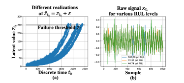
Figure 1: (a) Simulated latent variable $z_{t_{k}}$ and (b) raw high-frequency time series realizations $x_{t_{k}}$.

II-B An experimental dataset on accelerated fatigue of ball bearings

The dataset in [22] consists of run-to-failure experiments of a total of 17 bearings, loaded in 3 different conditions. Only 2-axis acceleration measurements are used in the present work. Temperature measurements are also available. Importantly, no artificial damage is introduced to the components for accelerating failure, thus rendering the accelerated testing scenario a better representation of real-world settings, where the failure mode is not known a-priori. The experimental conditions are summarized in Table II.

In order to test generalization on un-seen experiments a test-set containing whole experiments is used. A different train/test split is adopted from [22], which is detailed in Table II.

TABLE I: Available experiments and loading conditions.

Conditions $i$	$\dot{\phi}_{i}$ [rpm]	$F_{i}$ [kN]	Number of experiments
A	1800	4.0	7
B	1650	4.2	7
C	1500	5.0	3

TABLE II: FEMTO bearings dataset, training/test split

Set	Experiment	Conditions	Failure time [s]	Num. Obs.
Training	1_2	A	8700	871
	1_3	A	23740	2375
	1_4	A	14270	1428
	1_5	A	24620	2463
	2_1	B	9100	911
	2_5	B	23100	2311
	2_6	B	7000	701
	3_3	C	4330	434
Testing	1_1	A	28072	2803
	1_6	A	24470	2448
	1_7	A	22580	2259
	2_2	B	7960	797
	2_3	B	19540	1955
	2_4	B	7500	751
	2_7	B	2290	230
	3_1	C	5140	515
	3_2	C	16360	1637

Fatigue damage on roller bearings, manifests as frictional wear of the bearings and/or the surrounding ring. Empirically, higher lateral loads $F_{i}$ and rotational speeds $\dot{\phi}_{i}$ are associated with faster wear for bearings. The $\ddot{u}_{x}$ and $\ddot{u}_{y}$ accelerometer data are available in 0.1 second segments, sampled at 25.56kHz (2556 samples per segment). Temporal convolution networks are used, to automatically detect and use features that potentially are useful to tracking degradation in these experiments.

III Model Architectures

III-A GraphNets for arbitrary inductive biases

GraphNets (GNs) are a class of machine learning algorithms operating with (typically pre-defined) attributed graph data, which generalize several graph neural network architectures. An attributed graph, in essence, is a set of nodes (vertices) $V:\{\mathbf{v}_{1},\cdots\mathbf{v}_{k}\}$ and edges $E:\{(\mathbf{e}_{1},r_{1},s_{1})\cdots(\mathbf{e}_{k},r_{k},s_{k})\}$ where $\mathbf{e}_{k}\in\mathbb{R}^{N^{e}}$ and $\mathbf{v}_{i}\in\mathbb{R}^{N^{v}}$. Each edge is a triplet $(\mathbf{e}_{j},r_{j},s_{j})$ (or equivallently $(\mathbf{e},\mathbf{v}_{r_{j}},\mathbf{v}_{s_{j}})$) and it contains a reference to a receiver node $\mathbf{v}_{r_{j}}$, to a sender node $\mathbf{v}_{s_{j}}$ as well as a (vector) attribute $\mathbf{e}_{j}$. Self-edges, i.e. when $r_{i}:=s_{i}$ are allowed. In [1] a more general class of GraphNets is presented where global variables which affect all nodes and edges are allowed. A GN with no global variables consists of a node-function $\phi^{v}$, an edge function $\phi^{e}$, and an edge aggregation function $\rho^{e\rightarrow v}$. The function $\rho^{e\rightarrow v}$ should be (1) invariant to the permutation of its inputs and (2) able to accept a variable number of inputs. In the following this will be referred to as the edge aggregation function. Simple valid aggregation functions are $Min(\cdot)$, $Max(\cdot)$, $Sum(\cdot)$ and $Mean(\cdot)$. Inventing more general aggregation functions (for instance by combining them) and investigating how they affect the approximation properties of GNs is an active current research subject [23].

Ignoring global graph attributes, the GraphNet computation procedure is as detailed in algorithm 1. First, the new edge states are evaluated using the sender and receiver vertex attributes ($\mathbf{v}_{s_{i}}$ and $\mathbf{v}_{r_{i}}$ correspondingly) and the previous edge state $\mathbf{e_{i}}$ as arguments to the edge function $\phi^{e}$. The arguments of the edge function may contain any combination of the source and target node attributes and the edge attribute. Afterwards, the nodes of the graph are iterated and the incoming edges for each node are used to compute an aggregated incoming edge message $\mathbf{\bar{e}}^{\prime}_{i}$ The aggregated edge message together with the node attributes are used to compute an updated node state. Typically, small Multi-Layer Perceptrons (MLPs) are used for the edge and node GraphNet functions $\phi^{e}$ and $\phi^{v}$. It is possible to compose GN blocks by using the output of a GN as the input to another GN block. Since a single GN block allows only first order neighbors to exchange messages, GN blocks are composed as

$$GN_{K}(GN_{K-1}(\cdots(GN_{0}(G)\cdots)))=$$

$$GN_{K}\circ GN_{K-1}\circ\cdots\circ GN_{0}(G)$$

where “$\circ$” denotes composition. The first GN block may cast the input graph data to a lower dimension so as to allow for more efficient computation. The first GN block may have edge functions that depend only on edge states $\phi^{e_{0}}(\mathbf{e})$ and correspondingly node functions that depend only on node states $\phi^{u_{0}}(\mathbf{v})$. This is refered to a Graph Independent GN block and it is used as the type of layer for the first and the last GN block. The inner GN steps (i.e. $GN_{1}$ to $GN_{K-1}$) are full GN blocks, where message passing takes place. This general computational pattern is refered to as encode-process-decode [1]. The inner GN blocks may have shared weights, yielding smaller memory footprint for the whole model or different weights, ammounting to different GN functions that need to be trained for each level. Sharing weights and repeatedly applying the same GN block helps propagate and combine information from more connected nodes in the graph.

function GraphNetwork($E$, $V$)

     for $k\in\{1\ldots{}N^{e}\}$ do

         $\mathbf{e}_{k}^{\prime}\leftarrow\phi^{e}\left(\mathbf{e}_{k},\mathbf{v}_{r_{k}},\mathbf{v}_{s_{k}}\right)$ $\triangleright$ 1. Compute updated edges

     end for

     for $i\in\{1\ldots{}N^{n}\}$ do

         let $E^{\prime}_{i}=\left\{\left(\mathbf{e}^{\prime}_{k},r_{k},s_{k}\right)\right\}_{r_{k}=i,\;k=1:N^{e}}$

         $\mathbf{\bar{e}}^{\prime}_{i}\leftarrow\rho^{e\rightarrow v}\left(E^{\prime}_{i}\right)$ $\triangleright$ 2. Aggregate edges per node

         $\mathbf{v}^{\prime}_{i}\leftarrow\phi^{v}\left(\mathbf{\bar{e}}^{\prime}_{i},\mathbf{v}_{i},\right)$ $\triangleright$ 3. Compute updated nodes

     end for

     let $V^{\prime}=\left\{\mathbf{v}^{\prime}\right\}_{i=1:N^{v}}$

     let $E^{\prime}=\left\{\left(\mathbf{e}^{\prime}_{k},r_{k},s_{k}\right)\right\}_{k=1:N^{e}}$

     return $(E^{\prime},V^{\prime})$

end function

Algorithm 1 GN block without global variables [1].

In the present work, as is the case with RNNs [24] and causal CNNs [25], the causal structure of time series is also exploited, which is a good inductive bias for the problem at hand, although without requiring that the data is processed as a chain-graph or that the data are regularly sampled. Instead, an arbitrary causal graph for the underlying state is built, together with functions to infer the quantity of interest which is the remaining useful life of a component given a set of non-consecutive short-term observations.

III-B Incorporation of Causal Inductive Biases using GraphNets

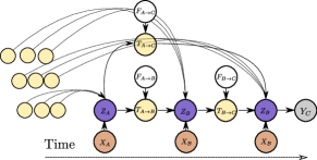
Figure 2: Dependency graph for the variables associated with the proposed model. $X_{A}$ represents the raw observed variable at time $t_{A}$. Variable $Z_{A}$ represents the (unobserved) state that can be translated to the quantity of interest $Y_{C}$ or a probabilistic estimate.

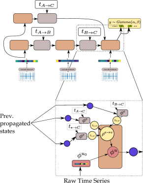
Figure 3: Detail of the GNN-tCNN. States are propagated with $\phi^{e}$ and accumulated with $\rho^{e\rightarrow u}$.

The variable dependencies of the proposed model are schematically depicted in Figure 2 for 3 observations. The computational architecture is depicted in more detail in Figure 3. The variable $Z_{K}$ represents the current estimate for the latent state of the system. The variable $T_{K\rightarrow L}$, which represents the propagated latent state from past observations, depends on the latent state $Z_{K}$, an exogenous input $F_{K\rightarrow L}$ that controls the propagation of state $Z_{K}$ to $Z_{L}$ and potentially other propagated latent state estimates from instants before $t_{L}$. The exogenous input $F_{K\rightarrow L}$ to the state propagation function can be as simple as the elapsed time between two time instants $t_{K\rightarrow L}=t_{L}-t_{K}$ or incorporate more prior inductive biases, such as the values representing different operating conditions during the interval between observations. An arbitrary number of past states can be propagated from past observations and aggregated in order to yield better estimates for a latent state $Z_{L}$. In adition to propagated latent states, instantaneous observations of raw data $X_{K}$ inform the latent state $Z_{K}$. For instance, in Figure 2 $Z_{C}$ depends on $T_{B\rightarrow C}$ but at the same time on $T_{A\rightarrow C}$ and potentially more propagated states from past observations (other yellow nodes in the graph) and at the same time to an instantaneous observation $X_{C}$. Each inferred latent state $Z_{i}$ can be transformed to a distribution for the quantity of interest $Y_{i}$. The value of the propagated state variable from state $s$ to state $d$, $T_{s\rightarrow t}$, depends jointly on the edge attributes and on the latent state of the source node. In a conventional RNN model, $F_{K\rightarrow L}$ corresponds to an exogenous input for the RNN cell. In contrast to an RNN model, in this work the dependence of the estimate of each state depends on multiple states by introducing a propagated state that is modulated by the exogenous input. In that manner an arbitrary and variable number of past states can be used directly for refining the estimate of the current latent state, instead of the estimate summarized in the latent cell state of the last RNN cell state. In the proposed model, the parameters of the functions relating the variables of the model are learned directly from data while only defining the inductive biases following naturally from the temporal ordering of the observations. This approach allows for uniform treatment of all observations from the past and allows for the consideration of an arbitrary number of such observations to yield an estimate of current latent state.

The connections from all observable past states and the ultimate one, where prediction (read-out) is performed, are implemented as a node-to-edge transformation and subsequent aggregations. Aggregation corresponds to the edge-aggregation function $\rho^{e\rightarrow u}(\cdot)$ of the GraphNet. In this manner, it is possible to propagate information from all distant past states on a single computation step. The computation of all available past states would be innefficient. To remedy that, it is possible to randomly sample the past states used in order to perform inference for the current step. Similarly, during training it is possible to yield unbiased estimates of gradients for the propagation and feature extraction model by randomly sampling the past states. It was found that for the presented use-cases this was an effective strategy for training. In GN terms, the “encode” GraphNet block ($GN_{enc}:\{\phi^{u_{0}},\phi^{e_{0}}\}$) is a graph-independent block consisting of the node function $\phi^{u_{0}}$ and edge function $\phi^{e_{0}}$. The node function is a temporal convolutional neural network (temporal CNNs), with architecture detailed in Table III.

TABLE III: Details on temporal CNN which acts as the node-function $\phi^{u_{0}}$ of the graph independent $GN_{enc}$ GraphNet. $n^{k},n^{s},n^{f}$ corresponds to kernel size, stride and number of filters. For dense layers $n^{f}$ corresponds to the layer width.

Layer type	$(n^{k},n^{s},n^{f})$	Activation
Conv1D	$(1\times 1,1,50)$	-
Conv1D	$(1\times 3,2,18)$	-
Conv1D	$(1\times 3,2,18)$	Dropout $20\%$ $ReLU$
Conv1D	$(1\times 3,2,50)$
Average Pool	$(1\times 2,2,1)$	-
Conv1D	$(1\times 1,1,50)$	-
Conv1D	$(1\times 3,2,18)$	-
Conv1D	$(1\times 3,2,18)$	Dropout $20\%$ $ReLU$
Conv1D	$(1\times 3,2,50)$	-
Avg. Pool	$(1\times 2,2,1)$	-
Conv1D	$(1\times 1,1,50)$	-
Conv1D	$(1\times 3,2,18)$	-
Conv1D	$(1\times 3,2,18)$	Dropout $20\%$ $ReLU$
Conv1D	$(1\times 3,2,50)$	-
Global Avg. Pool	$(1\times 2,2,1)$	-
Feed-forward	$(-,-,15)$	$Leaky\,ReLU$

The edge update function is a feed-forward neural network. The input of the edge function is the temporal difference between observations. Both networks cast their inputs to vectors of the same size. The $GN_{core}:\{\phi^{u_{c}},\phi^{e_{c}},\rho^{e\rightarrow u}\}$ network, consists of small feed-forward neural networks for the node MLP $\phi^{u_{c}}$ and the edge MLP $\phi^{e_{c}}$. The input of the edge MLP is the sender and receiver state and the previous edge state. The MLP is implemented with a residual connection to allow for better propagation of gradients through multiple steps [26].

$$\mathbf{e}^{\prime}_{i}\leftarrow\phi^{e_{c}}(\mathbf{e}_{i},\mathbf{u}_{s_{i}},\mathbf{u}_{r_{i}})=\bar{\phi}^{e_{c}}(\mathbf{e}_{i},\mathbf{u}_{s_{i}},\mathbf{u}_{r_{i}})+\mathbf{e}_{i}$$

In this work, the $Mean(\cdot)$ aggregation function was chosen, which does not depend strongly on the in-degree of the state nodes $Z_{i}$ (i.e. number of incoming messages) which corresponds to step $2$ in algorithm 1. The node MLP of the core network is also implemented as a residual MLP.

$$\mathbf{u^{\prime}}_{i}\leftarrow\phi^{u_{c}}(\mathbf{u}_{i},\mathbf{\bar{e}}_{i})=\bar{\phi}^{u_{c}}(\mathbf{u}_{i},\mathbf{\bar{e}}_{i})+\mathbf{u}_{i}$$

The $GN_{core}$ network is applied multiple times to the output of $GN_{enc}$. This ammounts to the shared weights variant of GNs which allow for propagation of information from multiple steps while costing a small memory footprint. After the last $GN_{core}$ step is applied, a final graph-independent layer is applied. At this point, for further computation only the final state of the last node is needed, which is the one corresponding to the last observation. The state of the last node is passed through two MLPs that terminate with $softplus$ activation functions

$$Softplus(x)=log(exp(x)+1).$$ (2)

The $Softplus$ activation is needed for forcing the outputs to be in $(0,+\inf)$, since they are used as parameters for a $Gamma$ distribution which in turn is used to represent the RUL estimates. The GraphNet computation procedure detailed above is denoted as

$$g_{out}=GN_{tot}(g)=GN_{dec}\circ GN_{core}^{(N_{c})}\circ GN_{enc}(g_{in})$$ (3)

where $GN_{core}^{(N_{c})}$ denotes $N_{c}$ compositions of the $GN_{core}$ GraphNet and “$g_{in},\,g_{out}$” are the input and output graphs. The vertex attribute of the final node is in turn used as rate ($\alpha(GN_{tot}(g_{in}))$) and concentration ($\beta(GN_{tot}(g_{in}))$) parameters of a $Gamma(\alpha,\beta)$ distribution. For ease of notation, the parameters (weights) of all the functions involved are denoted by “$\bm{\theta}$” and the functions that return the rate and concentration are denoted as $f_{\alpha;{\mathbf{\theta}}}$ and $f_{\beta;{\mathbf{\theta}}}$ correspondingly to denote explicitly their dependence on “$\bm{\theta}$”. The $Gamma$ distribution was chosen for the distribution of the output values since they correspond to remaining time and they are necessarily positive. The GN described above is trained so as to maximize directly the expected likelihood of the remaining useful life estimates. For numerical reasons, equivalently, the negative log-likelihood (nll) is maximized. The optimization problem reads,

$$\operatorname*{arg\,max}_{\bm{\theta}}\mathbb{E}_{(\mathcal{P},\mathcal{S})}[p(\mathbf{y}|\mathbf{g})]\propto\operatorname*{arg\,max}_{\bm{\theta}}\prod_{i=1}^{N^{s,p}}p(y_{i}|g_{i})\equiv$$

$$=\operatorname*{arg\,min}_{\bm{\theta}}\sum_{i=1}^{N^{s,p}}\Big{(}-\log p(y_{i}|f_{\alpha;\bm{\theta}}(g_{i}),f_{\beta;{\bm{\theta}}}(g_{i}))\Big{)}$$ (4)

where $\mathbf{g}$ corresponds to the sets of input graphs, and $\mathbf{y}$ corresponds to the estimate of RUL for the last observation of each graph. The input graphs in our case consist of nodes, which correspond to observations and edges with time-difference as their features. Correspondingly $g_{i}$ and $y_{i}$ are single samples from the aformentioned set of causal graphs and remaining useful life estimates and $N^{s,p}$ denotes the number of sampled causal graphs from experiment $p$ used for computing the loss (i.e. batch size). The expectation symbol is approximated by an expectation over the set of available training experiments denoted as $\mathcal{P}$ and the random causal graphs created for training $\mathcal{S}$. The gradients of Equation 4 are computable through implicit re-parametrization gradients [27]. This technique allows for low-variance estimates for the gradient of the nll loss with respect to the parameters of the distribution, which in turn allows for a complete end-to-end differentiable training procedure for the proposed architecture.

As in recurrent neural network models [29, 24], and [25], a gated-tanh activation function was used for the edge update and node update core networks.

$$h(y)=sigmoid(W_{g}y)\odot tanh(W_{a}y)$$

GraphNets using this activation strongly outperformed the ones using tanh but showed similar performance to the ones using relu activation. Networks for the edge and node MLPs were tested with widths $30,\,50,$ and $100$. The smaller networks tested (size $30$) consistently outperformed networks with size $50$ and for the most part had similar performance with networks with size $100$ for some cases. The $30-$unit networks were selected for the presented results.

III-C Recurrent Neural Network with Temporal CNN Feature Extractors (LSTM-tCNN)

The Causal GNN component of the architecture detailed in subsection III-B is used to satisfy the following desiderata: (1) to allow for computationally efficient and parallelized propagation of information from time-instants in the distant past with respect to the current timestep and (2) to allow for learning a state-propagation function and hence dealing with arbitrarily spaced points in a consistent manner. Although gated RNNs, such as GRUs and LSTMs, rely on sequential computation between timesteps, and therefore less parallelizeable, they are known to be relatively effective in dealing with long dependencies. Moreover, by appending the time difference between observations in the input gate of the RNN the RNN can learn to condition the predictions for the propagated state not only on the previous state and the CNN feature extractor input but also to the time-difference between different RNN steps [28]. One such model, using an LSTM cell, is depicted in Figure 4.

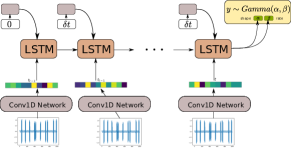
Figure 4: Model architecture of LSTM-tCNN.

IV Results

IV-A Simulated Dataset

Although it is easy to create a large number of training and test set experiments from the simulated dataset, in order to keep the simulated use-case realistic, only 12 experiments were used for training and a set of 3 experiments were used as a test set. Representative prediction results for the test-set experiments are shown in 5a. The accuracy of the model is inspected in terms of the expected negative log likelihood (smaller is better).When more observations are used, the estimates for the RUL of the fictitious processes are more accurate for a larger portion of the entirety of the observations. When a single observation is used, which completely neglects the long-term evolution of damage but uses short-term features extracted by the learned graph-independent $\phi^{u_{0}}$ which is a temporal CNN, the RUL estimates are inaccurate and fluctuate at the beginning of the experiment (top-right side of the first column of the plots). It is also observed that when using more observations, although the uncertainty bounds are not becoming smaller at the beginning of the fictitious experiment, the estimates of the trend of degradation, and consequently the remaining useful life of the component are accurate and smooth early on in the course of the experiment.

This observation provides evidence that the proposed architecture accurately captures both features of the high-frequency time series through the CNNs of the first graph-independent processing step, and the long-term evolution of the time series through the GraphNet processing steps. Moreover, the estimated probability distributions of RUL become more concentrated closer to failure, while they are wider at the beginning of the experiments. This observation aligns with the intuition that it is not possible to have sharp estimates in the beginning of the experiments.

IV-B Bearings Dataset

Results for representative experiments from the test-set of the FEMTO-bearing dataset are shown in 5b. Similarly to the simulated experiments, predictions are characterized by smaller uncertainty closer to failure and the degradation trends are captured effectively. Predictions employing up to 30 arbitrarily spaced observations from the past 2000 seconds are shown. Using more observations (more than 30) did not signifficantly improve the accuracy or the uncertainty bounds of the predictions. This may be due to the fact that the damage phenomenon is slowly evolving, thus using a larger number of points does not offer more information on the evolution of the phenomenon.

(a) GNN-tCNN, Simulated

(b) GNN-tCNN, Bearings

(c) LSTM-tCNN, Bearings

Figure 5: (a) Results on the simulated dataset using GNN-tCNN. (b), (c) Results on the bearing dataset using GNN-tCNN and LSTM-tCNN.

V Conclusion

Two neural network architectures (GNN-tCNN and RNN-tCNN) were applied to the problem of remaining life assessment on real-world experimental data and on artificial data from a stochastic degradation process. Both architectures seem to capture the long-term dependences on features of the considered time series. The GraphNet architecture proposed features a causal connectivity structure that can capture with less sequential computation long-term dependencies in the time series. Finally, an effective gradient-based technique, which employs low-variance reparametrization-based gradient estimators for fitting distributions with positive quantities of interest, such as RUL estimates, was employed. The proposed architectures are intuitive and easy to implement.

Although only RUL estimation problems were considered in this work, the non-sequential causal approach to dealing with long-term dependencies may be applicable to further applications where non-regularly sampled time series arise (e.g. electronic health records). In future works, other time-series tasks such as time-series generation or unsupervised/self-supervised learning [13] are to be attempted, employing the GNN-tCNN architecture.

Charilaos Mylonas was born in Thessaloniki, Greece. He holds a Dipl. Ing. Structural Engineering degree from Aristotle University of Thessaloniki and a MSc on Computational Science and Engineering from ETH Zürich. He previously worked as a scientific software developer at ETH Zürich and as a full-stack software developer in the banking sector. He is currently working towards his Ph.D. on the topic of remaining life assessment and uncerainty quantification for wind turbines.

Eleni Chatzi was born in Athens, Greece. She received her PhD (2010) from the Department of Civil Engineering and Engineering Mechanics at Columbia University. She is Chair of Structural Mechanics and Monitoring at the Department of Civil, Environmental and Geomatic Engineering of ETH Zürich. Her research interests include the fields of Structural Health Monitoring (SHM) and structural dynamics, nonlinear system identification, and intelligent assessment for engineered systems. She is leading the ERC Starting Grant WINDMIL on smart monitoring of Wind Turbines. Her work in the domain of self-aware infrastructure was recognized with the 2020 Walter L. Huber Research prize, awarded by the American Society of Civil Engineers (ASCE).

References

- [1] P. W. Battaglia, J. B. Hamrick, V. Bapst, A. Sanchez-Gonzalez, V. Zambaldi, M. Malinowski, A. Tacchetti, D. Raposo, A. Santoro, R. Faulkner et al., “Relational inductive biases, deep learning, and graph networks,” arXiv preprint arXiv:1806.01261, 2018.
- [2] J. Gilmer, S. S. Schoenholz, P. F. Riley, O. Vinyals, and G. E. Dahl, “Neural message passing for quantum chemistry,” arXiv preprint arXiv:1704.01212, 2017.
- [3] X. Wang, R. Girshick, A. Gupta, and K. He, “Non-local neural networks,” in Proceedings of the IEEE conference on computer vision and pattern recognition, pp. 7794–7803, 2018.
- [4] J. Sikorska, M. Hodkiewicz, and L. Ma, “Prognostic modelling options for remaining useful life estimation by industry,” Mechanical systems and signal processing, vol. 25, no. 5, pp. 1803–1836, 2011.
- [5] R. Razavi-Far, S. Chakrabarti, M. Saif, and E. Zio, “An integrated imputation-prediction scheme for prognostics of battery data with missing observations,” Expert Systems with Applications, vol. 115, pp. 709–723, 2019.
- [6] R. T. Chen, Y. Rubanova, J. Bettencourt, and D. K. Duvenaud, “Neural ordinary differential equations,” in Advances in neural information processing systems, pp. 6571–6583, 2018.
- [7] A. Voelker, I. Kajić, and C. Eliasmith, “Legendre memory units: Continuous-time representation in recurrent neural networks,” in Advances in Neural Information Processing Systems, pp. 15 570–15 579, 2019.
- [8] B. Raghavendra, D. Bera, A. S. Bopardikar, and R. Narayanan, “Cardiac arrhythmia detection using dynamic time warping of ecg beats in e-healthcare systems,” in 2011 IEEE International Symposium on a World of Wireless, Mobile and Multimedia Networks, pp. 1–6. IEEE, 2011.
- [9] D. Zhen, T. Wang, F. Gu, and A. Ball, “Fault diagnosis of motor drives using stator current signal analysis based on dynamic time warping,” Mechanical Systems and Signal Processing, vol. 34, no. 1-2, pp. 191–202, 2013.
- [10] B. Rouet-Leduc, C. Hulbert, N. Lubbers, K. Barros, C. J. Humphreys, and P. A. Johnson, “Machine learning predicts laboratory earthquakes,” Geophysical Research Letters, vol. 44, no. 18, pp. 9276–9282, 2017.
- [11] T. Kitamura, E. Hayahara, and Y. Simazciki, “Speaker-independent word recogniton in noisy environments using dynamic and averaged spectral features based on a two-dimensional mel-cepstrum,” in First International Conference on Spoken Language Processing, 1990.
- [12] Z. Yang, P. Baraldi, and E. Zio, “Automatic extraction of a health indicator from vibrational data by sparse autoencoders,” in 2018 3rd International Conference on System Reliability and Safety (ICSRS), pp. 328–332. IEEE, 2018.
- [13] A. Hyvarinen and H. Morioka, “Unsupervised feature extraction by time-contrastive learning and nonlinear ica,” in Advances in Neural Information Processing Systems, pp. 3765–3773, 2016.
- [14] L. Deng, M. L. Seltzer, D. Yu, A. Acero, A.-r. Mohamed, and G. Hinton, “Binary coding of speech spectrograms using a deep auto-encoder,” in Eleventh Annual Conference of the International Speech Communication Association, 2010.
- [15] B. Yang, R. Liu, and E. Zio, “Remaining useful life prediction based on a double-convolutional neural network architecture,” IEEE Transactions on Industrial Electronics, vol. 66, no. 12, pp. 9521–9530, 2019.
- [16] B. Wang, Y. Lei, T. Yan, N. Li, and L. Guo, “Recurrent convolutional neural network: A new framework for remaining useful life prediction of machinery,” Neurocomputing, vol. 379, pp. 117–129, 2020.
- [17] M. Liang and X. Hu, “Recurrent convolutional neural network for object recognition,” in Proceedings of the IEEE conference on computer vision and pattern recognition, pp. 3367–3375, 2015.
- [18] Y. Gal and Z. Ghahramani, “Dropout as a bayesian approximation: Representing model uncertainty in deep learning,” in international conference on machine learning, pp. 1050–1059, 2016.
- [19] B. Wang, Y. Lei, N. Li, and W. Wang, “Multi-scale convolutional attention network for predicting remaining useful life of machinery,” IEEE Transactions on Industrial Electronics, 2020.
- [20] J. Shi, T. Yu, K. Goebel, and D. Wu, “Remaining useful life prediction of bearings using ensemble learning: The impact of diversity in base learners and features,” Journal of Computing and Information Science in Engineering, vol. 21, no. 2, 2020.
- [21] J. L. Bogdanoff and F. Kozin, “A New Cumulative Damage Model - Part 4,” Journal of Applied Mechanics, vol. 47, DOI 10.1115/1.3153635, no. 1, pp. 40–44, 03 1980. [Online]. Available: https://doi.org/10.1115/1.3153635
- [22] P. Nectoux, R. Gouriveau, K. Medjaher, E. Ramasso, B. Chebel-Morello, N. Zerhouni, and C. Varnier, “Pronostia: An experimental platform for bearings accelerated degradation tests.” 2012.
- [23] G. Corso, L. Cavalleri, D. Beaini, P. Liò, and P. Veličković, “Principal neighbourhood aggregation for graph nets,” arXiv preprint arXiv:2004.05718, 2020.
- [24] S. Hochreiter and J. Schmidhuber, “Long short-term memory,” Neural computation, vol. 9, no. 8, pp. 1735–1780, 1997.
- [25] A. v. d. Oord, S. Dieleman, H. Zen, K. Simonyan, O. Vinyals, A. Graves, N. Kalchbrenner, A. Senior, and K. Kavukcuoglu, “Wavenet: A generative model for raw audio,” arXiv preprint arXiv:1609.03499, 2016.
- [26] K. He, X. Zhang, S. Ren, and J. Sun, “Deep residual learning for image recognition,” in Proceedings of the IEEE conference on computer vision and pattern recognition, pp. 770–778, 2016.
- [27] M. Figurnov, S. Mohamed, and A. Mnih, “Implicit reparameterization gradients,” in Advances in Neural Information Processing Systems, pp. 441–452, 2018.
- [28] Y. Zhu, H. Li, Y. Liao, B. Wang, Z. Guan, H. Liu, and D. Cai, “What to do next: Modeling user behaviors by time-lstm.” in IJCAI, vol. 17, pp. 3602–3608, 2017.
- [29] K. Cho, B. Van Merriënboer, C. Gulcehre, D. Bahdanau, F. Bougares, H. Schwenk, and Y. Bengio, “Learning phrase representations using rnn encoder-decoder for statistical machine translation,” arXiv preprint arXiv:1406.1078, 2014.