The Radio Luminosity-Risetime Function of Core-Collapse Supernovae

Abstract

We assemble a large set of 2–10 GHz radio flux density measurements and upper limits of 294 different supernovae (SNe), from the literature and our own and archival data. Only 31% of SNe were detected. We characterize the SN radio lightcurves near the peak using a two-parameter model, with $t_{\rm pk}$ being the time to rise to a peak and $L_{\rm pk}$ the spectral luminosity at that peak. Over all SNe in our sample at $D<100$ Mpc, we find that $\mbox{$t_{\rm pk}$}=10^{1.7\pm 0.9}$ d, and that $\mbox{$L_{\rm pk}$}=10^{25.5\pm 1.6}$ erg s^-1 Hz^-1, and therefore that generally, 50% of SNe will have $\mbox{$L_{\rm pk}$}<10^{25.5}$ erg s^-1 Hz^-1. These $L_{\rm pk}$ values are $\sim$30 times lower than those for only detected SNe. Types I b/c and II (excluding IIn’s) have similar mean values of $L_{\rm pk}$ but the former have a wider range, whereas Type IIn SNe have $\sim 10$ times higher values with $L_{\rm pk}$=$10^{26.5\pm 1.1}$ erg s^-1 Hz^-1. As for $t_{\rm pk}$, Type I b/c have $t_{\rm pk}$ of only $10^{1.1\pm 0.5}$ d while Type II have $t_{\rm pk}$=$10^{1.6\pm 1.0}$ and Type IIn the longest timescales with $t_{\rm pk}$$=10^{3.1\pm 0.7}$ d. We also estimate the distribution of progenitor mass-loss rates, $\dot{M}$, and find the mean and standard deviation of $\log_{10}(\mbox{$\dot{M}$}/[\mbox{M\raisebox{-2.58334pt}{$\odot$} yr${}^{-1}$}])$ are $-5.4\pm 1.2$ (assuming $v_{\rm wind}$=1000 km s^-1) for Type I b/c SNe, and $-6.9\pm 1.4$ (assuming $v_{\rm wind}$= 10 km s^-1) for Type II SNe excluding Type IIn.

1 Introduction

Core collapse supernova (SNe) can produce bright radio emission. The chief source of this emission is the interaction of the rapidly expanding ejecta with the circumstellar medium (CSM), which usually consists of the stellar wind of the SN progenitor, but may also have a significant contribution from mass-stripping in binary systems. Shocks are formed in this interaction, which serve to accelerate particles to relativistic velocities and amplify the magnetic field, resulting in synchrotron radio emission.

The radio emission provides us with a probe of the CSM, as well as for the outer, highest-velocity portion of the SN ejecta, for which few other observational probes are available. SNe are much less luminous in the radio than in the optical, with typical radio luminosities $<10^{-4}$ of those in the optical. Compared to the thousands of SNe detected in the optical, only $\sim$100 SNe have been detected in the radio. Furthermore, only core-collapse SNe have been detected to date, and as yet no Type Ia SN (for recent limits on the radio emission of Type Ia SNe, see Lundqvist et al., 2020). In this paper, therefore, we consider only core-collapse SNe, that is SN of Types Ib, Ic and II, and whenever we use the term “SN” we are referring only to ones of the core-collapse variety.

The radio emission from SNe is synchrotron emission. It generally displays a high brightness temperature, and a non-thermal spectrum. Their radio lightcurves follow a general pattern with a rise to a maximum, which can occur days to years after the SN explosion. The peak is followed by a decay, often of an approximately power-law form, with $S_{\nu}\propto t^{\beta}$, where $S_{\nu}$ is the flux density at frequency $\nu$, $t$ the time since the explosion, and $\beta$ is usually in the range of $-1$ to $-3$. As an illustration, we show the 8.4 GHz lightcurve of SN 1993J in Figure 1 (data from Bartel et al., 2002, and our own unpublished measurements). SN 1993J shows the typical rise and then power-law decay, although in this case, there is a distinct change in the slope of the decay after about 7 yr.

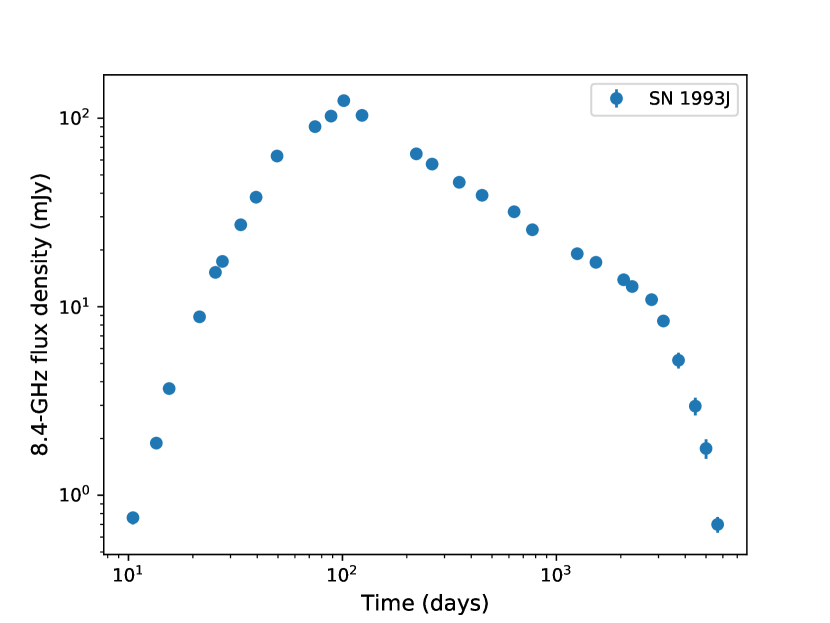
Figure 1: An example radio lightcurve of a core-collapse SN. We show the lightcurve of the Type IIb SN 1993J (data from Bartel et al. 2002; see also Martí-Vidal et al. 2011), which is one of the most intensively observed radio SNe. We plot the flux density, $S$, at 8.4 GHz against the time, $t$, since the explosion, with both axes being logarithmic. The errorbars are mostly smaller than the plotted points. The typical features are a rapid rise to a peak, which occurs at $\mbox{$t_{\rm pk}$}\simeq 130$ d with $S_{\rm pk}=123$ mJy, followed by a decline. In the case of SN 1993J the decline is of an approximately power-law form ($S\propto t^{-\beta}$), until $t\simeq 2500$ d, at which time there is a distinct steepening of the slope of the logarithmic decline. For our purposes here, we concentrate only on the region of the lightcurve near the peak and do not try to fit features such as the change in slope in the decay.

The radio lightcurves of SNe vary over a large range. Although the brightest SNe reach peak spectral luminosities, $L_{\rm pk}$ $=10^{29}$ erg s^-1 Hz^-1 (e.g., SN 1998bw, SN 2009bb), a considerable fraction of even nearby SNe are never detected in the radio, and must have $L_{\rm pk}$ values at least 3 orders of magnitude lower, or $<10^{26}$ erg s^-1 Hz^-1. Indeed, the $L_{\rm pk}$ of SN 1987A was another 2 orders of magnitude lower at $\lesssim 10^{24}$ erg s^-1 Hz^-1. Similarly, the risetimes $t_{\rm pk}$, have a very wide range. Some SNe, such as SN 1987A, have a very short $\mbox{$t_{\rm pk}$}\simeq 1$ d, while others, such as SN 1986J, can take several years to reach their peak.

A considerable number of radio flux density measurements of individual SNe have been published over the years. Much effort has also gone into parameterizing and modeling the radio lightcurves for the subset of SNe for which densely-sampled lightcurves are available (see e.g., Weiler et al., 2002). However, there has been rather less examination of the population as a whole. In this paper, we will explore, in a largely empirical way, the radio luminosity function of supernovae, and attempt first to answer the questions: how bright do we expect a core-collapse supernova to get in the radio, and how long do we expect it to take to reach this peak?

Our approach is as follows: we will adopt a simple parameterization of a supernova radio lightcurve, with only two parameters: $t_{\rm pk}$, the time between the explosion and $L_{\rm pk}$, the peak spectral luminosity at that time. The challenge is to find the values of $t_{\rm pk}$ and $L_{\rm pk}$. For a lightcurve with many flux density measurements as depicted in Figure 1 this can be done straightforwardly and relatively unambiguously. However, if there is only a single flux density measurement available, then the determination of $t_{\rm pk}$ and $L_{\rm pk}$ is ambiguous but as we will quantify later, the range of possible values of $t_{\rm pk}$ and $L_{\rm pk}$ is still well constrained. In the case of only upper limits on the flux density, the values of $t_{\rm pk}$ and $L_{\rm pk}$ are also ambiguous, but nonetheless still constrained, although generally less so than in the case of a single measurement. In this paper we use all our measurements to derive statistically meaningful results.

Many SNe in fact show behavior more complex than assumed in our simple model, with modulated lightcurves and anomalous rises at late times (for example, SN 1993J, already shown in Figure 1; but also SN 1979C, Bartel & Bietenholz 2008; SN 1986J, Bietenholz et al. 2002; SN 1987A, Zanardo et al. 2010; Cendes et al. 2018; SN 2001em Bietenholz & Bartel 2005; and SN 2001ig Ryder et al. 2004). However, most SNe do show an initial rise to a peak brightness and then a subsequent decay, so our model should suffice for giving us some insight into the population as a whole. For those SNe, such as SN 1987A, which showed a late-time rise in the radio emission, we use only the measurements for the first rise and subsequent decay.

We divide SNe into different Types such as Types I b/c or II and determine the difference in the luminosity-risetime function for different SN Types. We use the following three main classifications: Type I b/c, Type IIn, and then the remainder of the Type II’s. In what follows, when we mention Type II, we always mean Type II excluding the Type IIn. In addition, we examine separately the subset of Type I b/c SNe which has broad optical lines, which we call “BL”, and the Type IIb subset of Type II’s.

Type IIn SNe are those with narrow optical lines. They constitute $\sim$12% of all Type II SNe (Smith et al., 2011). Examples are SN 1986J and SN 1998S. These SNe are thought to be due to interaction with a dense CSM, which produces the narrow lines, and often strong radio emission. The radio evolution of Type IIn SNe is quite different from that of normal Type II SNe, which is why we treat then as a separate group. Occasionally Type Ib SNe are also observed to have narrow lines, and classed as Type Ibn. Our sample, however, contained only a single Type Ibn SN, SN 2015G, which was not detected, therefore we do not discuss the Ibn subtype separately.

We also discuss the subset of Type I b/c SNe which have broad optical lines, indicating high ejection velocities, (BL) as a group. This subtype has been of special interest because it is associated with gamma-ray bursts (Woosley & Bloom, 2006; Cano et al., 2017).

Finally, we also discuss the Type IIb subset of Type II SNe, of which SN 1993J is the most famous example. These SNe initially have H in their spectra and are therefore classified as Type II, but transition subsequently to having He-dominated spectra more characteristic of Type Ib. They constitute $\sim$14% of all Type II’s (Smith et al., 2011).

An important caveat must be mentioned here. The classification of SNe into Types is based on features in the optical spectrum. Since such features can vary as the SN evolves, there is the possibility that a SN may appear as different Types at different stages in its evolution. Indeed, we just mentioned the Type IIb SNe whose spectra changes from Type II to one resembling Type Ib.

The classification of Type IIn SNe is also occasionally time-variable. The interaction with the dense CSM giving rise to the narrow lines and the “n” characteristics can start only some time after the explosion, so some SNe might first appear to be normal Type I or II, and then develop the “n” characteristics. SN 2014C is a prominent example of this behavior, which started as a Type Ib but developed IIn characteristics after about 1 yr (Milisavljevic et al., 2015). SN 2001em is the other example of this behaviour in our sample. Since the dominant part of the radio lightcurve for both SN 2001em and SN 2014C occurs at later times, when the optical spectrum was of Type IIn, we classify both SNe as Type IIn.

Given the possible time-variability of the spectral characteristics, and therefore the non-uniqueness of the SN Type classification, our division by the SN Types is not completely unique. However, since only a small fraction of SNe show such time-variable spectral characteristics, our statistical results should not be greatly affected by their occurrence.

The remainder of this paper is organized as follows. First in Section 2, we briefly describe the observations and data reduction for the new data in this paper. Then, in Section 3, we describe our collection of radio measurements of 294 SNe. In Section 4 we describe the model of a SN radio lightcurve we fit to our measurements, which is characterized by only two parameters, $t_{\rm pk}$ and $L_{\rm pk}$. For many SNe, the measurements are not sufficient to uniquely determine the values of $t_{\rm pk}$ and $L_{\rm pk}$, for example, if there is only a single measurement, or only upper limits. In Section 5, we combine these constraints over all our SNe, and determine the likelihood of different values of $t_{\rm pk}$ and $L_{\rm pk}$ given our measurements. We then parameterize the distribution of $L_{\rm pk}$ and $t_{\rm pk}$, finding that lognormal form is the most likely, and proceed to determine the particular lognormal distributions for $t_{\rm pk}$ and $L_{\rm pk}$ which are most compatible with our measurements. We also examine various SN subtypes, such as Type I b/c and Type II, to ask whether the distribution of $t_{\rm pk}$ and $L_{\rm pk}$ differs for different SN Types. In Section 6, we use our distrutions of $t_{\rm pk}$ and $L_{\rm pk}$ to estimate the distribution of mass-loss rates. In Section 7, we discuss the implications of our results, and finally in Section 8 we summarize them and give our conclusions.

2 Observations and Data Reduction

We discuss our complete data-set which includes both published and previously unpublished values in the next section. Here we give a brief summary of the observations and data reduction of the 296 previously unpublished SN observations.

We re-reduced a number of archival observations of SNe from the Karl G. Jansky Very Large Array (VLA). This was done in a standard manner, using the Astronomical Image Processing System (AIPS; Associated Universities, 1999) for observations from the VLA before about 2011, and Common Astronomy Software Application (CASA; International Consortium Of Scientists, 2011) The flux density calibration was done using observations of 3C 48, 3C 138 or 3C 286. Phase self-calibration was done on the supernova observations in cases where the signal-to-noise ratio was adequate, but no amplitude self-calibration was done. In most of the archival data sets, the supernova was not detected, so no self-calibration was done.

The flux densities were determined by fitting to the images elliptical Gaussians, fixed to the dimensions of the restoring beam, along with a zero-level to account for any extended emission from the host galaxies. The total uncertainties (in Table 1) include a 5% uncertainty on the flux-density calibration, and in some cases a contribution from the uncertainty in separating the SN from the background emission, added in quadrature to the image background rms.

All observations with the Australia Telescope Compact Array (ATCA) used the 2 GHz bandwidth CABB system (Wilson et al., 2011) and were processed and measured using the miriad package (Sault et al., 1995), as described in Bufano et al. (2014). The primary flux density calibrator was PKS B1934-638, and no self-calibration was applied.

Observations with the Multi-Element Radio-Linked Interferometer Network (MERLIN) used the e-Merlin pipeline (Argo, 2014) using 512 MHz bandwidth. The primary flux density calibrator was 3C 286, and no self-calibration was done.

Table 1: Table: Supernova flux densities or limits from radio observations

Title: The Radio Luminosity-Risetime Function of Core-Collapse Supernovae
Authors: Bietenholz M.F., Bartel N., Argo M., Dua R., Ryder S., Soderberg A.
Table: Supernova flux densities or limits from radio observations
================================================================================
Byte-by-byte Description of file: datafile1.txt
--------------------------------------------------------------------------------
   Bytes Format Units   Label  Explanations
--------------------------------------------------------------------------------
   1-  9 A9     ---     ID     SN identifier
      11 A1     ---     Limit  [L] Limit flag on Flux (1)
  13- 16 I4     yr      Obs.Y  UT Year of observation midpoint
  18- 19 I2     month   Obs.M  UT Month of observation midpoint
  21- 25 F5.2   d       Obs.D  UT Day of observation midpoint
  27- 33 A7     ---     Tel    Telescope identifier (2)
  36- 40 F5.2   GHz     Freq   Observed frequency
  42- 49 F8.4   mJy     Flux   Measured flux density at Freq (3)
  51- 56 F6.4   mJy   e_Flux   Uncertainty in Flux
  58- 63 A6     ---     Com    Additional comment (4)
--------------------------------------------------------------------------------
Note (1): "L" indicates a limit, blank indicates a measured value.
Note (2):
    VLA = Very Large Array, USA; if known, the VLA configuration
          is appended,  e.g. VLA-A;
  MERLIN= the Multi-Element Radio-Linked Interferometer Network, UK;
    ATCA= Australia Telescope Compact Array, Australia.
Note (3): A negative value indicates a limit, with the magnitude of
          the value being the 3-sigma upper limit
Note (4): "Weiler" indicates that this value was retrieved from the
          website of the late Kurt Weiler.
--------------------------------------------------------------------------------
SN1980O   L 1988  2  1.32 VLA-AB    4.86  -0.360  0.120
SN1982F   L 1984  8 31.00 VLA-D     4.86  -1.160  0.390
SN1982F   L 1984 12 23.00 VLA-A     4.86  -0.180  0.060
SN1985F   L 1985  3 18.00 VLA       4.86  -0.189  0.064
SN1985F   L 1985  7 31.00 VLA       4.86  -0.330  0.110
SN1985G   L 1985  5  7.3  VLA       4.86  -0.212  0.071
SN1985G   L 1985  9  1.00 VLA       4.86  -0.675  0.225
SN1985G   L 1986 12 15.00 VLA       4.86  -0.623  0.208
....
SN1993N   L 1994  2 18.32 VLA       8.44  -0.110  0.037
SN1993N   L 1997  1 23.00 VLA       8.46  -0.186  0.062  Weiler
....
SN2010as    2010  4 16.7  ATCA      9.00   2.19   0.11
SN2010as    2010  4 25.5  ATCA      9.00   3.10   0.9
....

3 The Data-set

We avail ourselves of as many of the published results as possible, taking care to include any published upper limits in the cases of non-detection. To keep our data-set as uniform as possible, we restricted ourselves to measurements between 4 and 10 GHz since the most commonly used observing frequencies are 4.8 and 8.4 GHz, making an exception for SN 1987A, where only a very few measurements are available in the first years at those frequencies and we therefore use the more complete 2.3 GHz lightcurve. We add to the previously published values a number of previously unpublished measurements, which are listed in Table 1.

Our previously unpublished values include new measurements from the ATCA and MERLIN, as well as a number of results from re-reduced data from the Karl G. Jansky Very Large Array (VLA) available in the National Radio Astronomy Observatory (NRAO) data archive. There are a considerable number of such observations which were never published. Many SNe, even relatively nearby ones, are never detected in the radio. Such non-detections are much less likely to be published, therefore the sample of published values is likely to be biased towards detections and thus higher radio luminosities. We have therefore re-reduced a significant number of unpublished archival measurements, the majority of which are indeed non-detections.

Finally, we include values from the website of the late Kurt W. Weiler. Dr. Weiler obtained many radio observations of SNe during his illustrious career — see, for example, Weiler et al. (2002). Some of these were made available for a time on his website at the U. S. Naval Observatory, but were never formally published. We had retrieved some of those values from the website, which we now include also in our data set and in Table 1.

While the largest fraction of our assembled observations are from the VLA and ATCA, we also have measurements from a number of other telescopes including MERLIN, the Westerbork Synthesis Radio Telescope, the European VLBI Network, the Urumqi radio telescope and the Parkes-Tidbinbilla Interferometer.

In total we have 1475 measurements the flux density, or upper limits on it, for 294 SNe. For well observed SNe, such as SN 1993J (Figure 1) or SN 1986J, we have very well sampled lightcurves, with many measurements ($n=29$ and 39 respectively), allowing $t_{\rm pk}$ and $L_{\rm pk}$ to be accurately determined. For the majority of SNe, however, only one or two measurements are available, which thus provide only weak constraints on $t_{\rm pk}$ or $L_{\rm pk}$. In fact, in many cases, the observations yielded only upper limits on the SN’s flux density.

Of our 294 SNe, only 31% ($n=90$) are detected. For the remaining 69% ($n=204$) we have only upper limits on the flux density. The average number of measurements or limits per SN, detected or not, is 5.0. However, this number is skewed by the 9% ($n=26$) of well-observed SNe which have more than 12 measurements each. In fact, 35% ($n=104$) of our SNe have only a single measurement or limit. At least three observations are required to uniquely determine the peak of the lightcurve (one near, one before and one after the peak). Only 27% ($n=79$) of our SNe have three or more measurements or limits, although in many of those cases, they all occur after the peak, so that the peak is not determined.

Given this relatively modest number of measurements, compared to what is available in the optical, and the fact that our sample is of necessity heterogeneous and incomplete, we cannot provide a definitive radio luminosity function for supernovae. Nonetheless, we have a larger data set than has ever previously been assembled, and sufficiently large that some reasonably robust inferences can be drawn. It is crucial for this purpose to consider the non-detections as well as the published detections.

Table 2 gives some details of the SNe in our database. In order to determine luminosities, we need the distances, $D$, for our SNe. In most cases, we calculated $D$ from the recession velocity for the parent galaxy from the NASA/IPAC Extragalactic Database (NED), using the value corrected for our motion with respect to the cosmic microwave background, and infall to the Virgo cluster, to the Great Attractor and to the Shapley supercluster (Mould et al., 2000).

We use the latest values from the Planck collaboration, which are $H_{0}=67.4$ km s^-1 Mpc^-1, $\Omega_{\rm matter}=0.315$ and $\Omega_{\Lambda}=0.685$ (Planck Collaboration et al., 2020). Since our most distant (SN 2010ay) is at $D\simeq 300$ Mpc, and most SNe (89%) are at $D<100$ Mpc, the precise values adopted for the cosmological parameters do not significantly affect our results. For SNe closer than 30 Mpc, we use the mean of the redshift-independent distances from NED when available in preference to those calculated from the recession velocity.

Table 2: Supernovae Observed in Radio

SN Name	Type	Galaxy	Distance	Explosion	Number of	Detected	References
			($D$; Mpc)	date	measurements
SN 1979C	IIL	NGC 4321	16.2	1979 04 06	67	Y	1, 2
SN 1980K	IIb-L	NGC 6946	5.5	1980 10 25	69	Y	3, 4
SN 1980O	II	NGC 1255	17.9	1980 12 30	2		5, 6
SN 1981A	II	NGC 1532	17.9	1981 02 28	1		5
SN 1981K	II	NGC 4258	7.3	1981 07 31	30	Y	1
SN 1982F	IIP	NGC 4490	6.2	1982 02 24	2		6
SN 1982aa	?	NGC 6052	80.5	1979 08 16	11	Y	7
SN 1983I	Ic	NGC 4051	13.7	1983 04 25	2		8
SN 1983K	II	NGC 4699	19.7	1983 06 22	3		9
SN 1983N	Ib	NGC 5236	4.9	1983 06 29	15	Y	10
SN 1984E	IIL	NGC 3169	22.4	1984 03 29	4		9
SN 1984L	Ib	NGC 991	8.8	1984 08 10	3	Y	11
SN 1985F	Ib/c	NGC 4618	7.2	1984 03 30	2		6
SN 1985G	IIP	NGC 4451	20.9	1985 03 17	3		6
SN 1985H	II	NGC 3359	16.0	1985 04 12	2		6
SN 1985L	IIL	NGC 5033	16.5	1985 06 13	7	Y	12
SN 1986E	IIL	NGC 4302	16.8	1986 03 28	7	Y	13
SN 1986J	IIn	NGC 891	10.0	1983 03 14	39	Y	14, 15
SN 1987A	IIf	LMC	0.051	1997 02 23	8	Y	16
SN 1987F	IIn:	NGC 4615	79.6	1987 03 22	4		6
SN 1987K	IIb	NGC 4651	16.5	1987 07 31	2		6
SN 1988I	IIn	Leda 86944	178	1988 03 07	1		9
SN 1988Z	IIn	MCG+03-28-22	111	1988 12 01	26	Y	6, 17
SN 1989C	IIP	UGC 5249	32.1	1989 02 01	1		9
SN 1989L	II	NGC 7339	22.0	1989 05 04	3		6
SN 1989R	IIn	UGC 2912	80.1	1989 09 15	1		9
SN 1990B	Ic	NGC 4568	17.4	1990 01 18	8	Y	18
SN 1990K	II	NGC 150	23.4	1990 05 14	2		6
SN 1991G	IIP	NGC 4088	13.9	1991 01 23	2		6
SN 1991N	Ic	NGC 3310	18.1	1991 04 02	2		8, 19
SN 1991ae	IIn	MCG+11-19-18	138	1991 05 15	2		6, 9
SN 1991av	IIn	Anon J215601+0059	288	1991 09 15	3		9
SN 1992H	II	NGC 5377	35.1	1992 02 11	2		6
SN 1992ad	II	NGC 4411B	22.4	1992 06 30	5	Y	6, 20
SN 1992bd	II	NGC 1097	16.9	1992 10 12	5		6
SN 1993G	IIL	NGC 3690	53.1	1993 02 24	1		6
SN 1993J	IIb	M81	3.7	1993 03 28	29	Y	21
SN 1993N	IIn	UGC 5695	50.2	1993 04 15	2		6, 22
SN 1993X	II	NGC 2276	40.5	1993 08 22	1		6
SN 1994I	Ic	M51	7.9	1994 03 31	39		6, 19, 23
SN 1994P	II	UGC 6983	19.6	1994 01 20	3		6
SN 1994W	IIn-P	NGC 4041	25.4	1994 07 30	3		6, 22
SN 1994Y	IIn	NGC 5371	46.4	1994 07 09	1		6
SN 1994ai	Ic	NGC 908	15.6	1994 12 20	2		6, 19
SN 1994ak	IIn	NGC 2782	43.1	1994 12 24	1		6
SN 1995N	IIn	MCG-02-38-17	31.4	1994 07 04	18	Y	24
SN 1995X	II	UGC 12160	25.5	1995 08 03	4		22
SN 1995ad	II	NGC 2139	27.0	1995 09 22	1		22
SN 1996L	IIn	ESO 266-G10	157	1996 03 12	1		22
SN 1996N	Ib	NGC 1398	19.8	1996 03 09	3	Y	6, 19, 25
SN 1996W	II	NGC 4027	12.2	1996 04 10	3		6, 22
SN 1996ae	IIn	NGC 5775	19.9	1996 01 27	4		6, 22
SN 1996an	II	NGC 1084	19.1	1996 05 30	2		22
SN 1996aq	Ic	NGC 5584	21.8	1996 08 17	4		6, 19, 26
SN 1996bu	IIn	NGC 3631	10.3	1996 11 14	2		6
SN 1996bw	II	NGC 664	79.0	1996 11 30	1		22
SN 1996cb	IIb	NGC 3510	13.9	1996 12 12	3	Y	6, 27
SN 1996cr	IIn:	Circinus	3.8	1995 03 01	11	Y	28
SN 1997W	II	NGC 664	79.0	1997 02 01	2		6, 22
SN 1997X	Ib/c	NGC 4691	21.3	1997 01 25	3	Y	6, 19
SN 1997ab	IIn	Anon J095100+2004	53.9	1996 04 11	2		22
SN 1997db	II	UGC 11861	18.9	1997 08 02	3		6, 22
SN 1997dn	II	NGC 3451	27.1	1997 10 29	1		6
SN 1997dq	IcBL	NGC 3810	15.7	1997 10 13	3		22, 19
SN 1997ef	IbBL	UGC 4107	55.9	1997 11 20	2		6, 19
SN 1997eg	IIn	NGC 5012	47.6	1997 12 04	3	Y	29
SN 1997ei	Ic	NGC 3963	48.8	1997 11 20	1		22
SN 1998S	IIn	NGC 3877	14.9	1998 02 28	8	Y	6, 22, 30
SN 1998bm	II	IC 2458	24.7	1998 04 21	2		6
SN 1998bw	IcBL	ESO 184-82	41.4	1998 04 25	31	Y	31
SN 1998dl	IIP	NGC 1084	19.1	1998 08 02	2		22
SN 1998dn	II	NGC 337A	13.7	1998 08 19	2		22
SN 1999B	II	UGC 7189	31.2	1999 01 14	1		6
SN 1999D	II	NGC 3690	52.6	1999 01 16	2		6, 22
SN 1999E	IIn	Anon J131716-1833	119	1998 09 10	1		22
SN 1999cn	Ic	MCG+02-38-43	111	1999 06 14	1		22
SN 1999dn	Ib	NGC 7714	29.1	1999 08 15	1		6, 19
SN 1999eb	IIn	NGC 664	79.0	1999 10 02	1		6
SN 1999eh	Ib	NGC 2770	28.6	1999 07 26	2		8, 19
SN 1999el	IIn	NGC 6951	23.1	1999 10 20	2		6
SN 1999em	IIP	NGC 1637	11.5	1999 10 24	5	Y	6, 22, 32
SN 1999ev	IIP	NGC 4724	13.9	1999 11 07	1		6
SN 1999ex	Ic	IC 5179	53.3	1999 11 01	1		33
SN 1999gi	IIP	NGC 3184	12.4	1999 12 06	3		6
SN 1999go	II	NGC 1376	60.4	1999 12 18	1		6
SN 1999gq	IIP	NGC 4523	16.7	1999 12 23	1	Y	6
SN 2000C	Ic	NGC 2415	59.4	2000 01 01	1		19, 33
SN 2000F	Ic	IC 302	86.1	2000 01 29	1		19
SN 2000P	IIn	NGC 4965	30.2	2000 03 08	2		22
SN 2000S	Ic	MCG-01-27-20	138	1999 10 09	1		19
SN 2000cr	Ic	NGC 5395	61.3	2000 06 21	1		33
SN 2000ds	Ib/c	NGC 2768	20.5	2000 05 28	3		8, 19
SN 2000ew	Ic	NGC 3810	15.7	2000 11 21	1		6
SN 2000fn	Ib	NGC 2526	72.3	2000 11 09	1		33
SN 2000ft	?	NGC 7469	73.5	2000 07 19	7	Y	34
SN 2001B	Ib	IC 391	27.4	2000 12 31	3	Y	19, 33
SN 2001M	Ic	NGC 3240	57.3	2001 01 17	1		33
SN 2001ai	Ic	NGC 5278	121	2001 03 24	1		33
SN 2001bb	Ic	IC 4319	82.0	2001 04 22	2		19, 33
SN 2001ch	Ic	MCG-01-54-16	46.8	2001 03 24	1		19
SN 2001ci	Ic	NGC 3079	16.4	2001 04 21	3	Y	6, 19, 33
SN 2001ef	Ic	IC 381	40.2	2001 09 04	2		19, 33
SN 2001ej	Ib	UGC 3829	62.8	2001 09 09	2		19, 33
SN 2001em	IIn	UGC 11794	89.7	2001 09 12	8	Y	35, 36, 37
SN 2001gd	IIb	NGC 5033	17.5	2001 09 03	11	Y	38
SN 2001ig	IIb	NGC 7424	9.3	2001 12 03	23	Y	39
SN 2001is	Ib	NGC 1961	61.2	2001 12 19	1		19
SN 2002ap	IcBL	NGC 628	8.9	2001 02 28	9	Y	19, 40
SN 2002bl	IcPecBL	UGC 5499	77.5	2002 02 23	2		19, 33
SN 2002cj	Ic	ESO 582-05	113	2002 04 16	1	Y	33
SN 2002cp	Ib/c	NGC 3074	82.9	2002 04 20	2		19, 33
SN 2002dg	Ib	Anon J145716+0554	225	2002 05 29	2		19, 33
SN 2002dn	Ic	IC 5145	112	2002 06 08	1		19, 33
SN 2002gy	Ib/c:	UGC 2701	107	2002 10 13	1		33
SN 2002hf	Ic	MCG-05-03-20	82.9	2002 10 26	2		19, 33
SN 2002hh	II	NGC 6946	5.6	2002 10 31	8	Y	22, 41
SN 2002hn	Ic	NGC 2532	82.1	2002 10 26	1		33
SN 2002ho	Ic	NGC 4210	47.2	2002 11 01	2		19, 33
SN 2002hy	IbPec	NGC 3464	60.7	2002 10 28	2		19, 33
SN 2002hz	Ib	UGC 12044	82.9	2002 11 07	2		19, 33
SN 2002ji	Ic	NGC 3655	30.3	2002 10 19	3		19, 33, 42
SN 2002jj	Ic	IC 340	60.6	2002 10 13	2		19, 33
SN 2002jp	Ic	NGC 3313	59.6	2001 11 15	2		19, 33
SN 2002jz	Ic	UGC 2984	22.9	2001 12 14	1		33
SN 2003H	IbPec	NGC 2207	22.3	2003 01 08	3		6, 42
SN 2003L	Ic	NGC 3506	104	2001 01 01	40	Y	43
SN 2003bg	IcPecBL	MCG -05-10-15	19.3	2003 02 22	41	Y	44
SN 2003bu	Ic	NGC 5953	105	2003 03 03	2		8
SN 2003dr	Ib/c	NGC 5714	41.7	2004 04 10	3		8, 19, 42
SN 2003dv	IIn	UGC 9638	33.9	2004 04 16	1		6
SN 2003ed	II	NGC 5303A	25.2	2003 04 30	4	Y	6, 45
SN 2003el	Ic	NGC 5000	93.4	2003 05 11	1		19
SN 2003gd	IIP	NGC 628	8.6	2003 03 17	5		6
SN 2003gk	Ib	NGC 7460	48.5	2003 06 15	1		8
SN 2003ie	IIP	NGC 4051	13.7	2003 09 19	4		6, 22
SN 2003jd	IcPecBL	MCG -01-59-2	84.6	2003 10 10	4		8, 19
SN 2003jg	Ib/c	NGC 2997	9.0	2003 10 01	3		8, 42
SN 2003lo	IIn	NGC 1376	60.4	2003 12 31	1		6
SN 2004A	IIP	NGC 6207	17.0	2004 01 06	6		6
SN 2004C	Ic	NGC 3683	32.6	2003 12 23	3	Y	6, 8
SN 2004am	IIP	NGC 3034	3.8	2003 11 07	3		22, 46
SN 2004ao	Ib	UGC 10862	26.8	2004 02 21	1		8
SN 2004bm	Ic	NGC 3437	24.4	2004 04 17	2		6, 42
SN 2004bu	IcBL	UGC 10089	92.1	2004 05 14	1		8
SN 2004cc	Ic	NGC 4568	17.4	2004 05 23	8	Y	47
SN 2004dj	IIP	NGC 2403	3.4	2004 07 13	40	Y	48
SN 2004dk	Ib	NGC 6118	20.8	2004 07 30	10	Y	47
SN 2004et	IIP	NGC 6946	5.6	2004 09 22	19	Y	22, 49
SN 2004gq	Ib	NGC 1832	24.3	2004 12 08	21	Y	47
SN 2004gt	Ib/c	NGC 4038	21.1	2004 11 27	2		8, 42, 60
SN 2005E	Ib/c	NGC 1032	38.8	2005 01 04	1		8
SN 2005U	IIb	NGC 3690	53.1	2005 01 28	2		6
SN 2005V	Ib/c	NGC 2146	19.6	2005 01 01	5		6, 8, 42
SN 2005aj	Ic	UGC 2411	41.1	2005 02 09	2		8, 42
SN 2005at	Ic	NGC 6744	7.2	2005 03 05	2		50
SN 2005ay	IIP	NGC 3938	12.7	2005 03 21	4		6
SN 2005cs	IIP	M51	7.9	2005 06 27	5		51
SN 2005ct	Ic	NGC 207	58.6	2005 05 29	1		8
SN 2005cz	Ib	NGC 4589	35.7	2005 06 17	1		8
SN 2005da	IcBL	UGC 11301	74.4	2005 06 25	3		8
SN 2005dl	II	NGC 2276	20.4	2005 08 25	2		6
SN 2005ek	Ic	UGC 2526	73.0	2005 09 22	1		52
SN 2005gl	IIn	NGC 266	68.8	2005 10 26	1		22
SN 2005ip	IIn	NGC 2906	36.5	2005 10 27	3	Y	53
SN 2005kd	IIn	2MFGC 3318	69.4	2005 11 10	4	Y	6, 22, 54, 55
SN 2005kl	Ic	NGC 4369	29.7	2005 11 01	1		6
SN 2006aj	IcBL	2XMM J032139.6+165202	153	2006 02 18	17	Y	56
SN 2006be	II	IC 4582	40.6	2006 03 13	1		57
SN 2006bp	IIP	NGC 3953	16.6	2006 04 09	4		22, 58
SN 2006gy	IIn	NGC 1260	85.0	2005 08 20	8		6, 59, 60
SN 2006jd	IIn	UGC 4179	83.7	2006 10 07	11	Y	61
SN 2006my	IIP	NGC 4651	16.5	2006 08 01	2		22
SN 2006ov	IIP	NGC 4303	14.6	2006 10 26	2		6, 22
SN 2007C	Ib	NGC 4981	22.7	2006 12 28	2	Y	6
SN 2007Y	IbPec	NGC 1187	16.8	2007 02 14	7		42, 62
SN 2007ak	IIn	UGC 3293	69.6	2007 03 10	1		22
SN 2007bg	IcBL	Anon J114926+5149	155	2007 04 16	18	Y	63
SN 2007gr	Ib/c	NGC 1058	5.2	2007 08 13	9	Y	64
SN 2007iq	IcBL	UGC 3416	62.5	2007 08 01	2		8, 42
SN 2007ke	Ib	NGC 1129	76.7	2007 09 02	1		8
SN 2007kj	Ib/c	NGC 7803	79.3	2007 09 14	1		8
SN 2007pk	IInPec	NGC 579	73.4	2007 11 08	1		65
SN 2007rt	IIn	UGC 6109	107	2007 09 05	1		66
SN 2007ru	IcBL	UGC 12381	70.3	2007 11 25	2		8
SN 2007rz	Ic	NGC 1590	57.1	2007 11 19	2		8, 42
SN 2007uy	Ib	NGC 2770	28.6	2007 12 27	16	Y	67
SN 2008B	IIn	NGC 5829	94.5	2008 01 02	1		68
SN 2008D	Ib	NGC 2770	28.6	2008 01 09	21	Y	69
SN 2008X	IIP	NGC 4141	35.4	2008 01 14	2		6, 70
SN 2008aj	IIn	MCG+06-30-34	122	2008 02 12	1		71
SN 2008ax	IIb	NGC 4490	6.2	2008 03 03	24	Y	22, 72
SN 2008be	IIn	NGC 5671	142	2008 03 12	1		73
SN 2008bk	IIP	NGC 7793	3.9	2008 03 07	1		74
SN 2008bm	IIn	Leda 45053	155	2008 03 29	1		75
SN 2008bo	IIb	NGC 6643	19.1	2008 03 27	7	Y	22, 76
SN 2008du	Ic	NGC 7422	72.4	2008 06 30	1		42
SN 2008dv	Ic	NGC 1343	10.5	2008 05 26	2		8, 42
SN 2008ew	Ic	IC1236	99.5	2008 08 06	1		8
SN 2008gm	IIn	NGC 7530	53.0	2008 10 02	1		77
SN 2008hh	Ic	IC 112	85.0	2008 11 04	1		8
SN 2008hn	Ic	NGC 2545	54.2	2008 11 12	1		8
SN 2008ij	II	NGC 6643	19.1	2008 12 19	1		78
SN 2008im	Ib	UGC 2906	40.2	2008 12 15	1		8
SN 2008in	IIP	NGC 4303	14.6	2008 12 22	2		6, 79
SN 2008ip	IIn	NGC 4846	90.2	2008 12 31	1		80
SN 2008iz	?	M82	3.8	2008 02 20	25	Y	81
SN 2008jb	II	ESO 302-14	9.3	2008 11 11	1	Y	6
SN 2009E	IIP	NGC 4141	35.4	2008 01 01	1		6
SN 2009H	II	NGC 1084	19.1	2009 01 02	2		82
SN 2009N	IIP	NGC 4487	17.2	2009 01 24	2		82
SN 2009au	IIn	ESO 443-21	36.5	2009 03 07	1		83
SN 2009bb	IcBL	NGC 3278	43.5	2009 03 19	17	Y	84
SN 2009dd	II	NGC 4088	13.9	2009 04 12	3		6, 85
SN 2009eo	IIn	Leda 53491	212	2009 04 13	1		86
SN 2009fs	IIn	UGC 11205	256	2009 06 01	1		87
SN 2009gj	IIb	NGC 134	16.8	2009 05 31	3	Y	88
SN 2009hd	II	NGC 3627	9.6	2009 06 19	1		6
SN 2009ip	IIn	NGC 7259	28.1	2009 09 13	5	Y	89
SN 2009kn	IIn	MCG-03-21-06	74.6	2009 10 11	1		90
SN 2009mk	IIb	ESO 293-34	20.3	2009 12 15	4		91
SN 2010O	Ib	NGC 3690	53.1	2010 01 24	2		92
SN 2010P	?	NGC 3690	53.1	2010 01 10	7	Y	92
SN 2010ah	IcBL	Anon J114403+5541	230	2010 02 21	4		93
SN 2010al	IInPec	UGC 4286	80.6	2010 03 07	1		94
SN 2010as	IIb	NGC 6000	27.4	2010 03 16	10	Y	60, 95
SN 2010ay	IcBL	Anon J123527+2704	314	2010 02 22	3		96
SN 2010bh	IcBL	Anon J071031-5615	276	2010 03 16	7	Y	97
SN 2010br	Ib/c	NGC 4051	13.7	2010 04 10	1		98
PTF10vgv	IcBL	2MASX J22160156+4052065	63.8	2010 09 13	1		99
SN 2010id	II	NGC 7483	74.1	2010 09 15	1		100
SN 2010jl	IIn	UGC 5189A	53.3	2010 10 01	11	Y	101
SN 2010jp	IIn	Anon J061630-2124	44.8	2010 11 13	2		102
SN 2010kp	II	Anon J040341+7045	22.3	2010 11 30	2		6, 103
PTF10abyy	II	galaxy unknown	133	2010 12 06	1		104
SN 2011cb	IIb	IC 5249	36.0	2011 04 18	4	Y	60, 105
SN 2011dh	IIb	M51	7.9	2011 05 31	16	Y	106
PTF11iqb	IIn	NGC 151	55.1	2011 07 20	1		107
PTF11qcj	IcBL	Leda 2295826	135	2011 10 08	20	Y	108
SN 2011ei	II	NGC 6925	28.7	2011 07 25	11	Y	109
SN 2011hp	Ic	NGC 4219	22.1	2011 11 04	1		110
SN 2011hs	IIb	IC 5267	21.3	2011 11 06	10	Y	111
SN 2011ja	IIP	NGC 4945	4.2	2011 12 12	2	Y	112
SN 2012A	IIP	NGC 3239	9.7	2012 01 07	2		6
SN 2012ap	IcBL	NGC 1729	53.6	2012 02 05	3	Y	113
SN 2012au	Ib	NGC 4790	22.9	2012 03 03	3	Y	114
SN 2012aw	IIP	NGC 3351	10.0	2012 03 15	9	Y	115
PTF 12gzk	Ic	SDSS J221241.53+003042.7	63.4	2012 07 24	3	Y	116
SN 2013df	IIb	NGC 4414	18.1	2013 06 04	5	Y	117
SN 2013ej	IIP	NGC 628	8.6	2013 07 28	2	Y	6
SN 2013fs	IIP	NGC 7610	53.4	2013 10 06	2		118
SN 2013ge	Ib/c	NGC 3287	15.4	2013 11 07	3		119
iPTF13bvn	Ib	NGC 5806	24.7	2013 06 16	2		120
SN 2014C	IIn	NGC 7331	13.4	2013 12 30	14	Y	121
SN 2014ad	IcBL	Mrk 1309	28.9	2014 03 09	6		122
SN 2014bc	IIP	NGC 4258	14.1	2014 04 08	1		6, 123
SN 2014bi	IIP	NGC 4096	11.5	2014 04 22	2		6, 123
SN 2014eh	Ic	NGC 6907	51.8	2014 10 29	1		124
AT 2014ge	Ib	NGC 4080	15.5	2014 09 26	5	Y	125
SN 2015G	Ibn	NGC 6951	23.1	2015 02 27	3		126
SN 2015J	IIn	Anon J073505-6907	24.1	2015 04 26	5	Y	60, 127
iPTF15eqv	IIb/Ib	NGC 3430	26.5	2015 08 18	4		128
ASASSN-15oz	IIL	HIPASS J1919-33	34.6	2015 08 27	2	Y	129
PSN J22460504-1059484	Ib	NGC 7371	41.4	2015 07 10	1	Y	130
PSN J14102342-4318437	Ib	NGC 5483	18.5	2015 12 03	1	Y	131
SN 2016aqf	II	NGC 2101	16.1	2016 02 24	2	Y	132
SN 2016bas	IIb	ESO 163-11	42.4	2016 03 02	8	Y	60, 133
SN 2016bau	Ib	NGC 3631	10.3	2016 03 12	2	Y	6, 134
SN 2016coi	IcBL	UGC 11868	18.1	2016 05 24	7	Y	135
SN 2016cvk	IIn-pec	ESO 344-21	50.4	2016 06 13	1		136
SN 2016gfy	II	NGC 2276	20.4	2016 09 10	1		6
Spirits 16tn	?	NGC 3556	10.0	2016 05 05	2		137
SN 2017ahn	II	NGC 3318	39.8	2017 02 08	1		138
SN 2017eaw	IIP	NGC 6946	5.6	2017 05 12	4	Y	139
SN 2017gax	Ib/c	NGC 1672	11.8	2017 08 12	1		140
SN 2018ec	Ic	NGC 3256	40.3	2017 12 27	1		60
SN 2018ie	IcBL	NGC 3456	70.6	2018 01 05	1		141
SN 2018if	IcBL	SDSS J091423.85+493533.4	141	2018 01 19	1		141
SN 2018bvw	IcBL	SDSS J115244.11+254027.1	258	2018 04 25	4	Y	142
SN 2018cow	Icpec	CGCG 137-068	72.7	2018 06 16	7	Y	143
SN 2018gep	IcBL	SDSS J164348.22+410243.3	144	2018 09 09	3	Y	144
SN 2018lab	II	IC 2163	21.0	2018 12 29	1		145
SN 2019eez	II	NGC 2207	22.3	2019 04 26	1		146
SN 2019ehk	Ib	NGC 4321	16.2	2019 04 28	5		147
SN 2019ejj	II	ESO 430-20	11.5	2019 04 29	1		146
SN 2019esa	IIn	ESO 035-18	25.9	2019 05 05	1		146
SN 2019fcn	II	ESO 430-20	11.5	2019 05 03	1		146
SN 2019mhm	IIP	NGC 6753	50.6	2019 10 09	1		148
SN 2019qar	Ib/c-pec	NGC 7083	48.5	2019 09 10	1		149
SN 2020ad	II	IC 4351	28.8	2019 12 03	1		150
SN 2020oi	Ic	NGC 4321	16.2	2020 01 07	9	Y	151
SN 2020bvc	IcBL	UGC 09379	122	2020 02 04	2	Y	152
SN 2020fqv	Ib/c	NGC 4568	21.0	2020 03 31	1		153
SN 2020fsb	II	ESO 515-04	35.2	2020 04 02	1		153
SN 2020llx	II	NGC 7140	46.7	2020 05 29	1		154

Note. — Table 1 is published in its entirety in the machine-readable format. Only a portion is shown here for guidance regarding its form and content.

3.1 Observed Radio Lightcurves

We plot the observed values in the form of radio lightcurves (i.e., spectral luminosity curves), including any upper limits, for all our SNe with known Types in Figure 2. We then also separate the SNe by Type, and restrict our sample to those SNe at $D<100$ Mpc (except as noted below), and plot values for Type I b/c SNe in Figure 3, those for Type II SNe (excluding IIn’s) in Figure 4, and those for Type IIn SNe in Figure 5.

The subtype IIb seem to have brighter radio emission than the remainder of the Type II’s, and we plot the Type IIb’s separately from the other Type II’s in Figure 6.

Finally we plot the values for the “broad-lined” (BL) TYpe Ic SNe separately from the remainder of the Type I b/c in Figure 7. Since SNe-BL are rare, and we have only 6 detected examples at $D<100$ Mpc, we plot all 27 BL SNe in our sample, regardless of $D$.

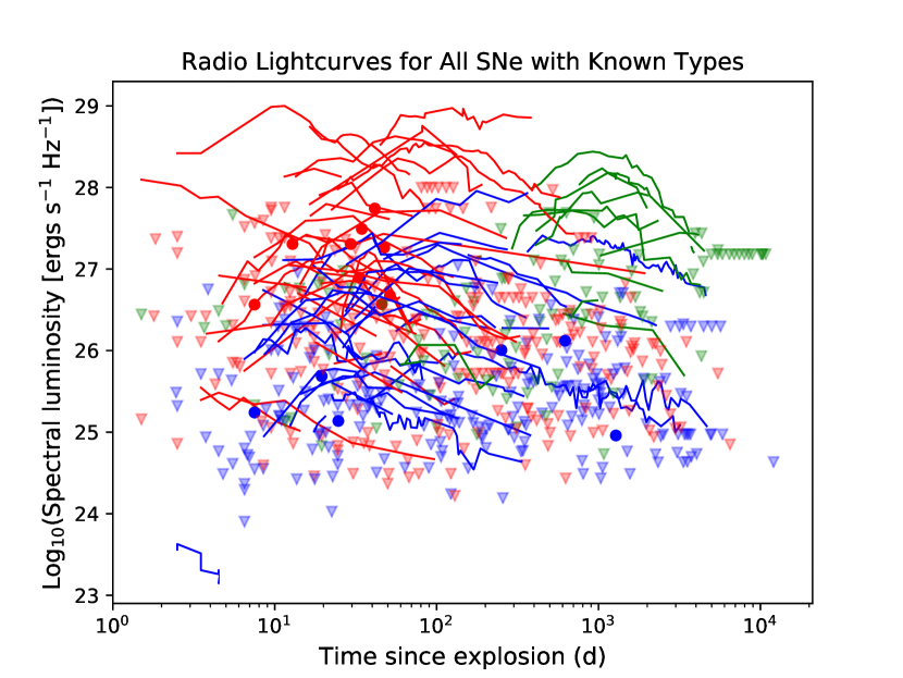
Figure 2: A plot of the measurements and lightcurves for all the 289 SNe in our sample with known SN Types. We plot the spectral luminosity against the time since the explosion, with both axes being logarithmic. The 129 Type I b/c SNe are plotted in red. The 53 SNe of Types IIn are plotted in green, and 107 remaining Type II’s in blue. The lines are lightcurves in the case of multiple detections, while the round points are single detections, and the pale triangles show upper limits. The lines do not show any fit, they just connect the available measurements. All measurements were between 4 and 10 GHz with the exception of SN 1987A. For SN 1987A, which is the lowest-luminosity curve in the plot, there were only very few early measurements available above 2.3-GHz, and we therefore use the more complete 2.3 GHz lightcurve.

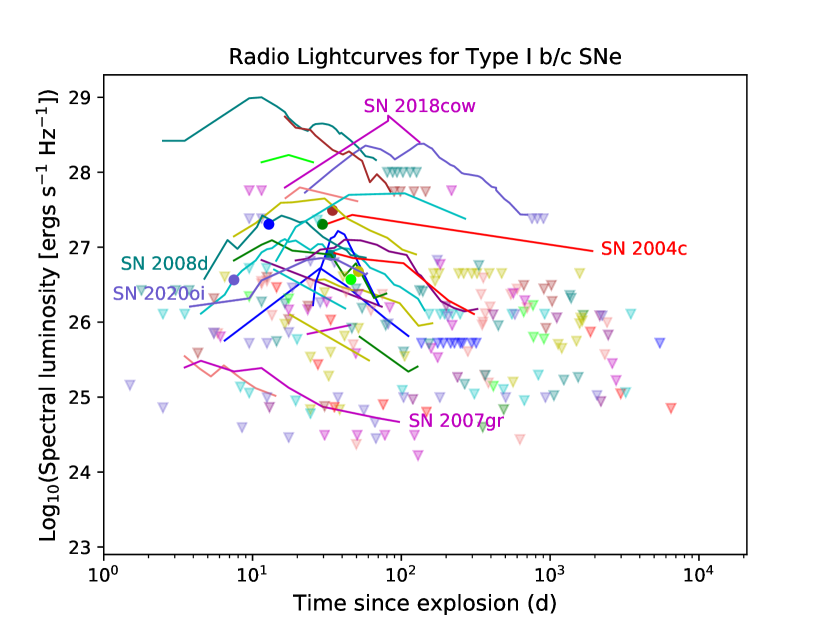
Figure 3: As Figure 2, but showing only the 110 SNe of Type I b/c and showing only those at $D<100$ Mpc. Different colors are used for the different SNe. The lightcurves for several SNe are labeled in the corresponding colors.

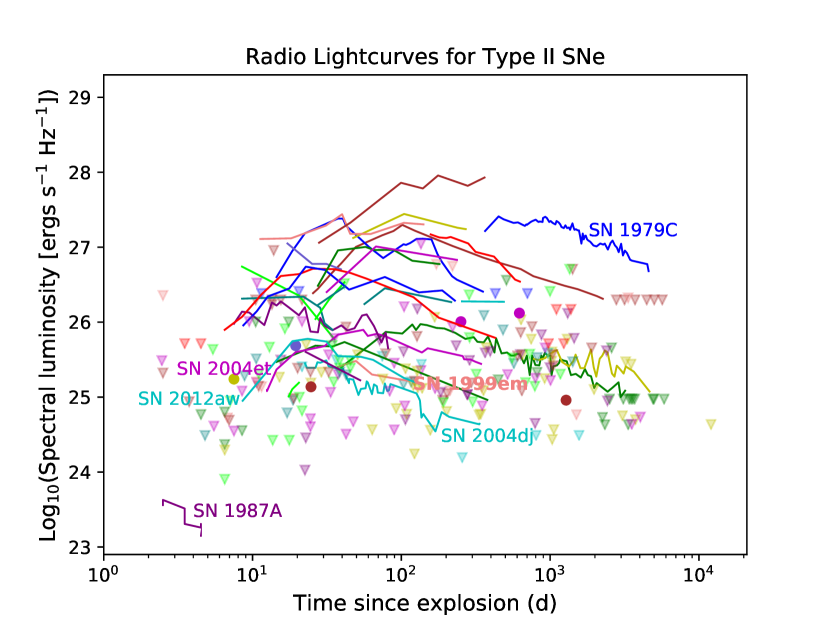
Figure 4: As Figure 2, but showing only the 106 SNe of Type II (excluding Type IIn) at $D<100$ Mpc. Different colors are used for the different SNe. The lightcurves for several SNe, including SN 1987A, are labeled in the corresponding colors. The lightcurve for SN 1987A is at 2.3 GHz, unlike all the others which are at 4 to 10 GHz.

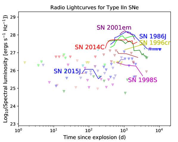
Figure 5: As Figure 2, but showing only the 41 SNe of Type IIn at $D<100$ Mpc. Different colors are used for the different SNe. The lightcurves for a few SNe are labeled in the corresponding colors. Since we treat values below 10% of the peak as upper limits (see Section 3), the trailing part of the SN 1986J lightcurve is indicated here as upper limits, though in fact the spectral luminosities are well measured (Bietenholz & Bartel, 2017b).

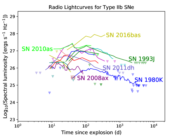
Figure 6: As Figure 2, but showing only the 19 SNe of Type IIb at $D<100$ Mpc. Different colors are used for the different SNe. The lightcurves for several SNe are labeled in the corresponding colors.

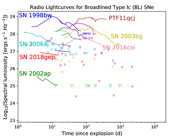
Figure 7: As Figure 2, but showing only the 27 broad-lined (BL) SNe (including those at $D>100$ Mpc). Different colors are used for the different SNe. We highlight the limits for SN 2014ad (Marongiu et al., 2019) with larger, lime-green triangles, since for that SN the measurements constrain the radio emission to low levels over a wide range of times.

A number of things are apparent from these figures. First, it can be seen that the lightcurves vary over a large range. $L_{\rm pk}$ can vary over more than 5 orders of magnitude, from $\sim\!10^{29}$ erg s^-1 Hz^-1 for SN 1998bw (Kulkarni et al., 1998), which is associated with GRB 980425, and SN 2009bb (Bietenholz et al., 2010b), to $<10^{24}$ erg s^-1 Hz^-1 for SN 1987A (Turtle et al., 1987). Similarly, some SNe, such as SN 1987A peak at $t_{\rm pk}$ $\lesssim 2$ d, while others such as SN 1986J have $\mbox{$t_{\rm pk}$}>1000$ d (Bietenholz et al., 2002), almost 3 orders of magnitude larger.

It can also be seen that the lightcurves exhibit a wide variety of forms. While generally they do show an initial rise and a subsequent decay of approximately power-law form, various “bumps” and changes in the slope of the power-law decay are seen.

Figure 2 shows that Type I b/c (red) reach the highest peak luminosities, followed by the Type IIn (green), while those of Type II SNe (blue) are lower. Type I b/c’s are more likely to peak earlier, while the Type II’s are likely to peak later and the Type IIn even later. This pattern has been noted earlier, for example in Weiler et al. (2002), but with only a relatively small sample of SNe. While we only have a single example detected at a low value of $\mbox{$L_{\rm pk}$}<10^{24}$ erg s^-1 Hz^-1 (SN 1987A, at $D$ only $\sim$50 kpc), which was of Type II, the distribution of upper limits for Type I b/c SNe is not obviously different than that for Type II’s, implying that low values of $\mbox{$L_{\rm pk}$}<10^{25}$ erg s^-1 Hz^-1 likely occur for both Type I b/c and II SNe. Type IIb SNe tend to have higher values of $L_{\rm pk}$ than the remainder of the Type II’s, and are therefore more likely to be detected. The Type Ic-BL SNe also tend to have high values of $L_{\rm pk}$  but note that some Ic-BL SNe, such as SN 2002ap and SN 2014ad have fairly low values of $L_{\nu}\lesssim 10^{25.5}$ erg s^-1 Hz^-1.

4 Lightcurve Modeling

4.1 The Model

As mentioned, in our model for the lightcurves, the spectral luminosity, $L_{\nu}$, of the SN rises to a peak, and then decays in a power-law fashion with $L_{\nu}\propto t^{\beta}$, where we take $\beta=-1.5$. Our model has only two free parameters, $t_{\rm pk}$, the time from the explosion to reach the peak, and $L_{\rm pk}$, the peak spectral luminosity.

The rise in the lightcurve is caused by an optical depth, $\tau$, which decreases as a function of time. This optical depth could be due to either external free-free absorption or internal synchrotron self-absorption, or a combination of the two. The peak in the lightcurve occurs approximately when $\tau=1$. We take $\tau\propto t^{-\delta}$ and $\delta=1$, which is a value which fits most SNe moderately well, although we explore different rise parameterizations in Section 7.4 below.

We fixed the slope of the power-law decay at $\beta=-1.5$ for all SNe. Different well-observed SNe do in fact show different values of $\beta$: For example, SN 1993J has a flatter decay particularly during the first $\sim$1000 d (Figure 1 and Bartel et al., 2002), while SN 1986J shows a steeper decay (Bietenholz & Bartel, 2017b). However, for our purposes, an average value of $\beta=-1.5$ gives a reasonable fit near the peak of the lightcurve.

Our model lightcurve, normalized so that it reaches $L_{\rm pk}$ at $t_{\rm pk}$, therefore has the form

$$L(t)=\mbox{$L_{\rm pk}$}\cdot 4.482\cdot e^{-1.5(t_{\rm pk}/t)}\cdot(t/\mbox{$t_{\rm pk}$})^{-1.5}.$$

As can be seen in Figure 2, the lightcurves of individual SNe are often more complex than our simple model. However, our model gives an adequate fit to the peak in the lightcurve, and thus serves our purpose here of providing an approximate, but sufficient, parameterization of SN lightcurves in general.

While more complex models are certainly warranted for studying individual SNe, and would likely yield more accurate values for $t_{\rm pk}$ and $L_{\rm pk}$, our purpose here is to examine the distribution of $t_{\rm pk}$ and $L_{\rm pk}$ over all SNe, so the approximate values obtained from our simple model are adequate. In particular, the fitted distributions of $t_{\rm pk}$ and $L_{\rm pk}$ depend only very weakly on the choice of parameterization for the rise and fall of the lightcurve, so even in cases where the shape of the actual lightcurve differs from the model, our fitted values for $t_{\rm pk}$ and $L_{\rm pk}$ should be adequate to our purpose.

In cases where we have many measurements, clearly those near to $t_{\rm pk}$ provide the best constraints on $t_{\rm pk}$ and $L_{\rm pk}$. Values that are either much earlier or much later than $t_{\rm pk}$ and well below $L_{\rm pk}$ provide little additional constraint on $t_{\rm pk}$ and $L_{\rm pk}$, and could drive the fitted values to deviate from the peak in the actual lightcurve in cases where our model is not a good match for the actual lightcurve shape. To minimize this effect, for any given SN, we downweight any measurements that are at $<10$% of the observed peak by treating them as upper limits. Note that we downweight measurements in this way only in cases where we have better measurements available for the same SN, that is those with $>10\,\times$ higher flux density. The effect of this is two-fold: firstly any “bumps” in the lightcurve that happen well below the peak have little effect on our fitted values of $t_{\rm pk}$ and $L_{\rm pk}$, and secondly, it serves to smooth the likelihood function in the $t_{\rm pk}$-$L_{\rm pk}$ plane slightly, which reduces the effect of our relatively coarse sampling in this plane.

An example of this can be seen in the case of SN 1993J, where the slope of the decay changes. Figure 1 shows the full set of 8.4-GHz measurements for SN 1993J, while the left panel of Figure 9 below shows the values that we used to fit $t_{\rm pk}$ and $L_{\rm pk}$ in this case, with the flux-densities $<10$% of the peak treated as upper limits.

4.2 Estimates of $t_{\rm pk}$ and $L_{\rm pk}$

For many of our SNe, particularly if only upper limits were obtained, the measurements do not determine a unique set of values of $t_{\rm pk}$ and $L_{\rm pk}$. Instead, some ranges of values are allowed and others excluded. In order to establish the distribution of $t_{\rm pk}$ and $L_{\rm pk}$ over our sample, we proceed in a Bayesian fashion as follows. We define a 2-dimensional array of possible values of $t_{\rm pk}$ and $L_{\rm pk}$. We choose logarithmically spaced values of $t_{\rm pk}$ and $L_{\rm pk}$ in view of the large range these quantities can take on. Then, for each SN, we calculate the likelihood of obtaining the flux-density measurements for that SN as a function of $t_{\rm pk}$ and $L_{\rm pk}$ (assuming the distance given in Table 2). If the likelihood is high for some particular pair of values $t_{\rm pk}$ and $L_{\rm pk}$, then a lightcurve characterized by those values of $t_{\rm pk}$ and $L_{\rm pk}$ represents a good fit to the measurements of the spectral luminosity.

Some values of $t_{\rm pk}$ and $L_{\rm pk}$ are un-physical: the frequency at which the spectrum turns over due to synchrotron self-absorption (SSA) depends only on the luminosity and size of the source. A lower limit on the size of the source can therefore be estimated from the observing frequency and value of $L_{\rm pk}$ (see Chevalier & Fransson, 2006). Assuming a spherical source, this size can be expressed as a radius, which we call the SSA-radius, $r_{\rm SSA}$. In the case that absorbing mechanisms other than SSA are active, for instance free-free absorption (FFA) in the CSM, the turnover frequency could be higher, so the source could be larger, but not smaller than calculated assuming only SSA, so $r_{\rm SSA}$, is a lower limit on the physical radius. The speed, $\mbox{$v_{\rm SSA}$}=r_{\rm SSA}/\mbox{$t_{\rm pk}$}$ is therefore a lower limit on the source’s expansion speed. Projection effects do allow apparent velocities somewhat larger than $c$ in the case of relativistic SNe, as were observed in SN 2003dh / GRB 030329 (Pihlström et al., 2007), but highly superluminal values are not expected. To exclude physically unlikely cases where highly relativistic expansion would be required, we therefore assign a likelihood of 0 to all points in the $t_{\rm pk}$, $L_{\rm pk}$ plane for which $\mbox{$v_{\rm SSA}$}>2c$. Although we use a non-relativistic calculation for $v_{\rm SSA}$, which will not provide accurate values when $\mbox{$v_{\rm SSA}$}\gtrsim c$, our cut at $\mbox{$v_{\rm SSA}$}>2c$ should nonetheless serve to exclude the majority of the physically unlikely combinations of $t_{\rm pk}$ and $L_{\rm pk}$. (Indeed, there are no well-determined values of $t_{\rm pk}$ and $L_{\rm pk}$ in this part of the plane.)

We show three examples of these likelihood arrays in Figure 8, and three examples of the possible lightcurves in Fig 9.

The first example is for a well-sampled case like SN 1993J (e.g., Bartel et al., 2002), Figure 8 left. The many luminosity measurements allow for only one specific fit of our model, which narrowly constrains the possible pairs of values of $t_{\rm pk}$ and $L_{\rm pk}$ and only one specific pair, corresponding to a single pixel in the $t_{\rm pk}$, $L_{\rm pk}$ plane, has a significantly non-zero likelihood. Only a single lightcurve fits the measurements in Figure 9 left.

The second example is for a supernova with only a single detection like PSN J22460504-1059484 (Kamble et al., 2015), shown in Figure 8 center. In this case many lightcurves are possible, all of them going through the sole luminosity measurement but some having the measured luminosity on the rising part and some on the falling part of the model lightcurve. In this case the allowed pairs of values of $t_{\rm pk}$ and $L_{\rm pk}$ are constrained to a thin curve. A family of related lightcurves, all passing through the single measurement, fit in Figure 9 center.

The third example is for a case where only one single upper limit of a luminosity measurement is available, like for SN 2017gax (Bannister et al., 2017), shown in Figure 8 right. Here the range of lightcurves with high likelihood is the largest, with many points in the $t_{\rm pk}$-$L_{\rm pk}$ plane having almost the same high likelihood, but still a portion of the plane is excluded. A range of lightcurves, constrained only by having to go below the observed limit, fit in Figure 9 right.

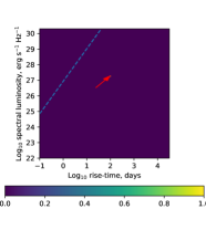
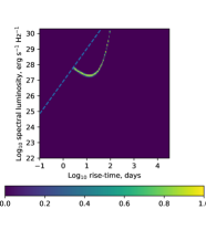
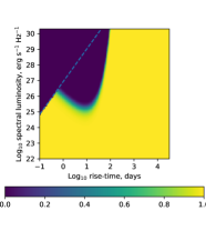
Figure 8: Plots of the likelihood of pairs of $t_{\rm pk}$ and $L_{\rm pk}$ values for three example SNe. The likelihoods are normalized to a maximum value of unity. The horizontal axis is $t_{\rm pk}$, while the vertical one is $L_{\rm pk}$, and the likelihood is shown in color. The values of $t_{\rm pk}$ and $L_{\rm pk}$ that imply an apparent expansion speed $>2c$ are excluded, which results in the region above the dashed line, at the top left of the plots, always having zero likelihood. Left: SN 1993J, for which many measurements tightly constrain the possible values of $t_{\rm pk}$ and $L_{\rm pk}$ to a region smaller than our resolution in the $t_{\rm pk}$, $L_{\rm pk}$ plane, and thus to a single pixel in the image, which is indicated by the red arrow. Middle: PSN J22460504-1059484, for which there was only a single measurement, but the SN was detected, thus constraining the possible locations in the $t_{\rm pk}$-$L_{\rm pk}$ plane to the thin curved line, occupying only a small part of the plane. The pixellation of the curved region is an artefact of our relatively low resolution in the $t_{\rm pk}$, $L_{\rm pk}$ plane, but should not significantly affect our results. Right: SN 2017gax, for which a single measurement yielded only an upper limit to the flux density. Many parts of the $t_{\rm pk}$-$L_{\rm pk}$ plane are therefore almost equally likely.

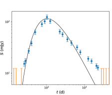
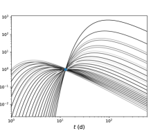
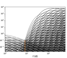
Figure 9: Plots of the possible lightcurves for the three example SNe. The darkness of the line indicates the relative likelihood of the measurements for that particular lightcurve. The errorbars indicate the $p=68$% ($1\sigma$) confidence limits in the case of both measured values (blue) and limits (orange). The lightcurves (in mJy) are calculated using the distances given in Table 2. Left: SN 1993J. The measurements (including the limits) have a high likelihood only for a single lightcurve defined by a particular set of $t_{\rm pk}$, $L_{\rm pk}$ values. In this case, one can see that modeled lightcurves do not match the measurements precisely, with the measurements suggesting a slightly slower rise, as well as a flatter decay, especially at $t>1000$ d, than our simple two-parameter model. However, the model reasonably reproduces the peak of the lightcurve. Note also that the measurements plotted as lower limits here were in fact detections (see Figure 1). As we explain in Section 3, we treat all values below 10% of the brightest observed value as upper limits so as to not unduly influence the fits near the peak. Middle: PSN J22460504-1059484. The measurements have a high likelihood for a range of related lightcurves, in some cases (with small values of $t_{\rm pk}$) placing the single measurement during the rise, and in others (with larger values of $t_{\rm pk}$) placing it during the decay. Right: SN 2017gax. The measurements have a high likelihood for a wide range of lightcurves, but nonetheless some lightcurves, e.g., those having $S_{\rm peak}\gtrsim 0.1$ mJy and $t_{\rm pk}$$\sim 5$ d, are excluded by the measurements.

5 The Radio Luminosity-Risetime Function, or the Distribution of $t_{\rm pk}$ and $L_{\rm pk}$

5.1 The Distribution of the Observed Values of $t_{\rm pk}$ and $L_{\rm pk}$

We want to determine the distribution of $t_{\rm pk}$ and $L_{\rm pk}$, which is the radio luminosity-risetime function for core-collapse SNe. To guide our investigation, we start first with the subset of SNe that have well-determined values of $t_{\rm pk}$ and $L_{\rm pk}$, which is the subset of examples similar to SN 1993J in Figures 8 and 9. We adopt simple observational values of $t_{\rm pk}$ and $L_{\rm pk}$ here, where $L_{\rm pk,obs}$ is the $L_{\nu}$ corresponding to the highest measured flux density, provided that the highest value was not either the first or the last measurement, and $t_{\rm pk,obs}$ is the time since the explosion of that measurement. Note that these observational values of $t_{\rm pk,obs}$ and $L_{\rm pk,obs}$ will generally not be identical to the values of $t_{\rm pk}$ and $L_{\rm pk}$ that have the highest likelihood from the previous section, since the latter are influenced by all the measured values, not just the single highest measurement. However, the maximum likelihood values of $t_{\rm pk}$ and $L_{\rm pk}$ should be similar to $t_{\rm pk,obs}$ and $L_{\rm pk,obs}$. We will return below to the fitted values of $t_{\rm pk}$ and $L_{\rm pk}$, which are required for the majority of SNe for which $t_{\rm pk,obs}$ and $L_{\rm pk,obs}$ are not determined. First however, we plot a scattergram of the observed values of $t_{\rm pk,obs}$ and $L_{\rm pk,obs}$ in Figure 10. As already noted in Figure 2, SNe of Type I b/c (shown in red) tend to have higher values of $L_{\rm pk}$ and lower values of $t_{\rm pk}$ than do Type II.

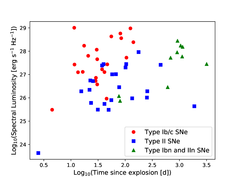
Figure 10: The observed values of the log₁₀ of the peak spectral luminosity, $L_{\rm pk,obs}$, against the time in days at which it occurs, $t_{\rm pk,obs}$, for all 54 SNe for which these values were determined. These values are not derived from any lightcurve fit to the measurements, but for each SN are merely the largest value of $L_{\nu}$ that was observed and the time it was observed. We do not plot SNe for which the highest observed value was the earliest (or only) one, since in those cases the peak cannot be determined. The interacting SNe, of Type IIn are shown as green triangles, while the remainder of the Type I b/c SNe are shown as red circles and the remainder of the Type II SNe are shown as blue squares. The isolated square at the lower left corner is SN 1987A. Many SNe for which only upper limits on the flux density could be determined would likely fall in the range below $L_{\rm pk}$ $<10^{25}$ erg s^-1 Hz^-1.

In Figure 11 we plot the histograms showing distributions of $t_{\rm pk,obs}$ and $L_{\rm pk,obs}$. For both, the values are scattered relatively uniformly in logarithmic space, suggesting that parameterizing the distributions of $t_{\rm pk}$ and $L_{\rm pk}$ in logarithmic space. Only for 57 SNe, (19% of our total of 294), can the values of $t_{\rm pk,obs}$ and $L_{\rm pk,obs}$ be determined.

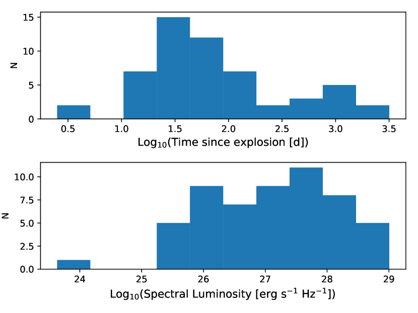
Figure 11: Histograms of the observed values of the log₁₀ of the time in days at which the observed peak occurred, $t_{\rm pk,obs}$, (top), and the spectral luminosity of that peak, $L_{\rm pk,obs}$ (bottom) for all 57 SNe for which these values were determined. See Figure 10 for the description of $t_{\rm pk,obs}$ and $L_{\rm pk,obs}$. These histograms represent only the population of detected, well-observed, SNe, and are not representative of the overall population, of which 69% is not detected. In particular, the distribution of $L_{\rm pk,obs}$ is strongly biased by exclusion of SNe for which only limits on $L_{\nu}$ were obtained. The mean of $t_{\rm pk,obs}$ was 1.88, and the standard devotion was 0.67, while the corresponding values for $L_{\rm pk,obs}$ were 27.09 and 1.09.

It is important to note that the histograms in Figure 11 represent only the population of well-observed, detected SNe, and are not representative of the overall population at $D<100$ Mpc, of which 69% was never detected and 80% do not have well-defined values of $t_{\rm pk,obs}$ and $L_{\rm pk,obs}$.

The most obvious bias is in the distribution of $L_{\rm pk,obs}$: If one were to take into account the 69% of SNe for which only upper limits on $L_{\nu}$ were ever obtained, many of them would be at $\mbox{$L_{\rm pk}$}<10^{25}$ erg s^-1 Hz^-1, and the distribution of $L_{\rm pk,obs}$ must therefore be biased towards higher values than the distribution of $L_{\rm pk}$ over all SNe. Indeed, only for SN 1987A could a value of $\mbox{$\log_{10}(\mbox{$L_{\rm pk}$})$}<25$ have been observed.

As far as $t_{\rm pk}$ is concerned, very few SNe are observed at all at times $<1$ week, therefore many SNe could lie in the range $\mbox{$t_{\rm pk}$}<10$ d, and the distribution in Figure 11 may be significantly biased here also.

5.2 The Distribution Function for $L_{\rm pk}$ and $t_{\rm pk}$ From All SNe

We now turn to incorporating the 80% of our sample for which $t_{\rm pk,obs}$ and $L_{\rm pk,obs}$ were not defined, which includes the 69% of SNe for which only upper limits on $L_{\nu}$ could be determined. Although the observations for these SNe do not determine $t_{\rm pk}$ or $L_{\rm pk}$ uniquely, they do provide some constraints on their possible values. We incorporate them by examining the likelihood of various values of $t_{\rm pk}$ and $L_{\rm pk}$ given the observations.

In Section 4.2, we calculated the likelihoods for each SN for different pairs of values of $t_{\rm pk}$ and $L_{\rm pk}$, with examples being shown in Figure 8. If we normalize these likelihood functions, they become the probability, $p_{i}(\mbox{$t_{\rm pk}$},\mbox{$L_{\rm pk}$})$, of SN number $i$, having some particular pair of $t_{\rm pk}$ and $L_{\rm pk}$ values (in Bayesian terms, this is equivalent to incorporating a flat prior for $t_{\rm pk}$ and $L_{\rm pk}$ to form the posterior probability). If we then sum these arrays over all of our SNe and divide by our total number of SNe (294), we arrive at the probability for particular pairs of values of $t_{\rm pk}$, $L_{\rm pk}$ over all of our SNe, $p_{\rm tot}(\mbox{$t_{\rm pk}$},\mbox{$L_{\rm pk}$})$. We show $p_{\rm tot}(\mbox{$t_{\rm pk}$},\mbox{$L_{\rm pk}$})$ in Figure 12.

The probability of different values of $t_{\rm pk}$ and $L_{\rm pk}$ is hard to interpret from Figure 8. On the one hand, there are a small number of SNe that have well-determined $t_{\rm pk}$ and $L_{\rm pk}$ (those in Figure 10 that produce a small number of high-probability pixels in Figure 8). As mentioned, these constitute an almost certainly biased subset of only 19% of our sample. On the other hand, there are many SNe for which the sparse measured values or limits mean that large areas of the $t_{\rm pk}$-$L_{\rm pk}$ plane have low, but significantly non-zero probability. Pairs of $t_{\rm pk}$-$L_{\rm pk}$ values which are physically unlikely, such as $\log_{10}(\mbox{$t_{\rm pk}$})$= 4, $\log_{10}(\mbox{$L_{\rm pk}$})$= 30, have non-zero probability because for many SNe they are not excluded by the measurements.

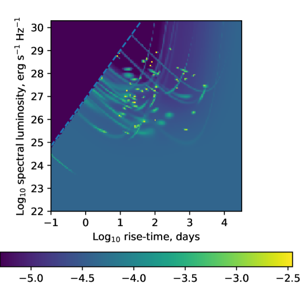
Figure 12: The logarithm of the probability, $\log_{10}[\mbox{$p_{\rm tot}$}(\mbox{$t_{\rm pk}$},\mbox{$L_{\rm pk}$})]$ of the measurements as a function of $t_{\rm pk}$ and $L_{\rm pk}$ over all our SNe. The maximum value of $p_{\rm tot}$ is 0.0039, which is approximately $1/(N_{\rm SNe}=294)$. For a small number of SNe (e.g., SN 1993J, Figure 8 left), the values of $t_{\rm pk}$ and $L_{\rm pk}$ are well determined, and therefore some particular pair of values has $p_{i}\simeq 1$, thus contributing $1/N_{\rm SNe}$ to $p_{\rm tot}$. For other SNe, allowed values of $p_{\rm tot}$ lie on curved lines, whose peak values will be lower than $1/N_{\rm SNe}$ (since $p_{i}$ must sum to 1 over the whole image). Finally, for SNe for which only upper limits are available, the maximum $p_{i}$ is lower still since it is spread out more or less uniformly over the bottom part of the $t_{\rm pk}$-$L_{\rm pk}$ plane. Although the probability for any particular $t_{\rm pk}$ and $L_{\rm pk}$ in this region is low, the integral of $p_{\rm tot}$ below, say, $\mbox{$L_{\rm pk}$}=10^{25}$ erg s^-1 Hz^-1 is substantial, so that the probability of $\mbox{$L_{\rm pk}$}<10^{25}$ erg s^-1 Hz^-1 is not negligible. Again, the region with $\mbox{$p_{\rm tot}$}=0$ at the top left above the dashed line is excluded because it would require strongly superluminal expansion.

To proceed we want to impose some reasonable constraints on the distributions of $t_{\rm pk}$ and $L_{\rm pk}$, for example considering extreme values unlikely even if they are allowed by our measurements. So, instead of attempting to estimate the probability distributions of $t_{\rm pk}$ and $L_{\rm pk}$ from Figure 8, we will proceed by hypothesizing some functional forms for the distributions. Although there is no physical reason to expect that the values of either $L_{\rm pk}$ or $t_{\rm pk}$ are in fact drawn from any distribution with a simple functional form, determining approximate forms of the distributions of $t_{\rm pk}$ and $L_{\rm pk}$ should prove useful until more physically-motivated versions can be found, for example, for estimating the likelihood of detecting future SNe in the radio. It also allows us to compare the distributions across different types of SNe, and may also provide some insight into the physics of radio emission from SNe.

We have noted in Section 5.1 that the values of both $t_{\rm pk}$ and $L_{\rm pk}$ seem relatively uniformly scattered in logarithmic space. A normal distribution in, for example, $t_{\rm pk}$ therefore seems incompatible with the measurements, whereas a normal distribution in $\log(\mbox{$t_{\rm pk}$})$, that is, a lognormal distribution in $t_{\rm pk}$, could provide a reasonable fit. We will therefore mostly work with the logarithms of $t_{\rm pk}$ and $L_{\rm pk}$, which we denote by $\mbox{$\log_{10}(\mbox{$t_{\rm pk}$})$}=\log_{10}(\mbox{$t_{\rm pk}$}/{\rm d})$ and $\mbox{$\log_{10}(\mbox{$L_{\rm pk}$})$}=\log_{10}(\mbox{$L_{\rm pk}$}/[\mbox{erg~{}s${}^{-1}$ Hz${}^{-1}$}])$.

Since there is no strong correlation between the more probable values of $t_{\rm pk}$ and $L_{\rm pk}$ in Figure 12, we consider only separate distributions for $t_{\rm pk}$ and $L_{\rm pk}$, so the hypothesized joint probability for $t_{\rm pk}$ and $L_{\rm pk}$ can be obtained by multiplying their respective hypothesized probability distributions. This product would be the anticipated radio luminosity-risetime function for core-collapse SNe.

5.3 Finding the Most Likely Distribution Function for $L_{\rm pk}$ and $t_{\rm pk}$

We try therefore the following three forms for the distribution functions for $\log_{10}(\mbox{$t_{\rm pk}$})$ and $\log_{10}(\mbox{$L_{\rm pk}$})$:

• 1. A uniform distribution in $\log_{10}(x)$ where $x$ is either $t_{\rm pk}$ or $L_{\rm pk}$. This distribution has two free parameters, namely the low and high limits, $x_{\rm low}$ and $x_{\rm high}$. (With well determined values of $t_{\rm pk}$ and $L_{\rm pk}$ the highest probability would be achieved by placing these limits at just below the smallest and just above the highest observed values. However, given that our measurements do not uniquely determine $t_{\rm pk}$ or $L_{\rm pk}$ in the majority of cases, the boundaries are flexible, and we determine the values of the limits that give the highest probability.)

• 2. A lognormal distribution in $x$, which is a normal distribution in $\log_{10}(x)$. This has also two free parameters, the mean, $\mu$, and the standard deviation, $\sigma$, so the probability, $p(x)=\frac{1}{\sigma\sqrt{(2\pi)}}e^{-0.5(\frac{x-\mu}{\sigma})^{2}}$.

• 3. A power-law distribution, where $p(x)=Kx^{q}$ if $x>x_{\rm min}$ and $p=0$ otherwise. This distribution also has two free parameters, namely $q$ and $x_{\rm min}$. Given that Figures 10 and 11 suggest that both very small and large values of $t_{\rm pk}$ are unlikely, we consider the power-law distribution only for $L_{\rm pk}$, where the many lower limits means small values of $L_{\rm pk}$ could be likely.

In all cases we normalize the distributions over the ranges $-1<\mbox{$\log_{10}(\mbox{$t_{\rm pk}$})$}<10^{4.5}$ (0.1 d to 86 yr) and $22<\mbox{$\log_{10}(\mbox{$L_{\rm pk}$})$}<30.3$ ($10^{22}$ to $2\times 10^{30}$ erg s^-1 Hz^-1).

For each SN, we then multiply the likelihood function for $t_{\rm pk}$ and $L_{\rm pk}$ (Figure 8) by the hypothesized joint distribution of $t_{\rm pk}$ and $L_{\rm pk}$. The integral of this product over all possible values of $t_{\rm pk}$ and $L_{\rm pk}$ then gives the likelihood of the measurements for this SN for this particular hypothesized $t_{\rm pk}$, $L_{\rm pk}$ distribution. The likelihood of the measurements for all SNe given the hypothesized distributions of $t_{\rm pk}$ and $L_{\rm pk}$ is then the product of the likelihoods for the individual SNe.

Our first goal is to determine which functional form, i.e., lognormal, uniform, or power-law, is most appropriate for $t_{\rm pk}$ and $L_{\rm pk}$. Since our sample is almost certainly notably incomplete at larger distances, we use here only those SNe at $D<100$ Mpc, where our sample is more complete, retaining 262 SNe from our total of 294.

We evaluate in a brute-force fashion the likelihood for each possible value of the four free parameters over the two distributions (two in $t_{\rm pk}$ and two in $L_{\rm pk}$; for example $\mu$ and $\sigma$ in the case of a lognormal distribution). We find that the highest likelihood occurs for lognormal distributions in both $t_{\rm pk}$ and $L_{\rm pk}$. The maximum-likelihood estimate of the lognormal distribution function for $\log_{10}(\mbox{$t_{\rm pk}$})$ has mean, $\mu=1.7$ and standard deviation $\sigma=0.9$, while that for $L_{\rm pk}$ has $\mu=25.5,\sigma=1.5$.

We give the values of the maximum likelihoods for other combinations of distribution functions relative to that for the best-fitting case of lognormal distributions in both $t_{\rm pk}$ and $L_{\rm pk}$, along with the associated parameter estimates in Table 3. A lognormal distribution in both $t_{\rm pk}$ and $L_{\rm pk}$ results in a significantly higher likelihood than any other combination of the three functions (lognormal, power-law, uniform) that we tried.

Table 3: Distribution Functions for $t_{\rm pk}$ and $L_{\rm pk}$

Distribution functions		Maximum likelihood
$t_{\rm pk}$	$L_{\rm pk}$	$\Delta\log_{10}p$	best-fit parameters
lognormal	lognormal	0	log_10$t_{\rm pk}$: μ=1.7, σ= 0.9;0log_10$L_{\rm pk}$: μ=25.5, σ=1.5
lognormal	power-law	-4.34	log_10$t_{\rm pk}$: μ=1.7, σ= 0.9;0log_10$L_{\rm pk}$: min=23.9, exponent=-1.24
uniform	lognormal	-5.11	log_10$t_{\rm pk}$: min$-0.3$, max=3.5;0log_10$L_{\rm pk}$: μ=25.6, σ=1.5
lognormal	log-uniform	-5.63	log_10$t_{\rm pk}$: μ=1.8, σ= 0.9;0log_10$L_{\rm pk}$: min=22.0, max=29.1

5.4 The Lognormal Distributions for Different SN types

Thus guided towards the use of lognormal distributions, we proceed to determine the distributions of $t_{\rm pk}$ and $L_{\rm pk}$ for various groups of SNe, to study whether different kinds of SNe are characterized by different distributions of $t_{\rm pk}$ and $L_{\rm pk}$. In addition to the maximum likelihood estimates of the means and standard deviations of the lognormal distributions, we also obtain the $p=68$% points, being the points where the overall likelihood is 68% of that associated with the best-fit values. We give our results in Table 4.

Are different Types of SNe characterized by different distributions of $t_{\rm pk}$ and $L_{\rm pk}$? We have already seen from Figure 2 that Type I b/c SNe tend to have higher $L_{\rm pk}$ and shorter $t_{\rm pk}$. We split our set of SNe by Type as discussed in our introduction, and fit the distributions of $t_{\rm pk}$ and $L_{\rm pk}$ separately for the different Types. We use the following three main classes: Type I b/c, Type IIn, and the remainder of the Type II’s. We also examine the subset of Type I b/c SNe that are broad-lined Type Ic (Ic-BL) and the Type IIb subset of the Type II SNe. The results are given in Table 4, and we plot the distributions in Figure 13.

Because of the completeness considerations mentioned earlier, we again consider only subsamples of SNe at $D<100$ Mpc, with the exception of the rare BL subclass, where we include all examples regardless of $D$. Note that the first line of Table 4 represents the same fit as the first line of Table 3.

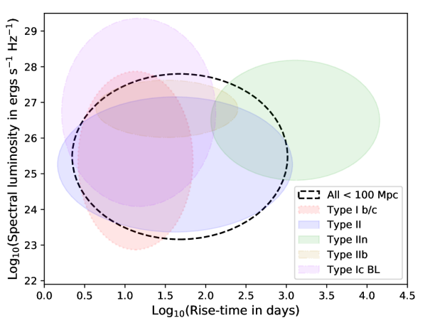
Figure 13: The distributions of different Types of SNe in the $t_{\rm pk}$, $L_{\rm pk}$ plane. The ellipses show the $p=68$% contour, i.e., the contour containing 68% of the SNe, of the relevant most-likely lognormal distributions for the various kinds of SNe (see Table 4). We illustrate the distributions for different samples of SNe as: All (dashed, black, $n=262$), Type I b/c (red, $n=110$), all Type II (except Type IIn; blue, $n=106$), Type IIn (green, $n=41$), Type IIb (mustard, $n=19$), and Type Ic-BL SNe (magenta, $n=27$). We use the samples at $D<100$ Mpc, except for the rare Type Ic BL where we take all examples regardless of $D$. Note that the Type IIb and Ic BL distributions are rather uncertain because of the small number of SNe.

We find that the 110 Type I b/c SNe are characterized by values of $t_{\rm pk}$ $\sim\!3\times$ lower and values of $L_{\rm pk}$ $\sim\!1.3\times$ higher than are the 106 Type II SNe. The range of $L_{\rm pk}$ values is higher for Type I SNe ($\sigma$ of $\log_{10}(\mbox{$L_{\rm pk}$})$= 1.7) than for Type II’s ($\sigma$ of $\log_{10}(\mbox{$L_{\rm pk}$})$= 1.3).

Type I b/c are over-represented in our sample, they form 42% of our sample at $D<100$ Mpc, while they represent only 26% of all the SNe in the Lick Observatory Supernova Search (LOSS; Smith et al., 2011) and 19% of a complete nearby sample of 175 SNe from LOSS (Li et al., 2011). The reason for the over-representation is that Type I b/c’s were more actively observed because of the potential association with GRBs.

We ask whether the presence of the Type II SN 1987A, which was clearly unusual in a number of respects, and which, because of its low radio luminosity, could be detected because of its nearness, biases our derived distributions of $t_{\rm pk}$ and $L_{\rm pk}$? We redid the fit for the 105 Type II SNe excluding SN 1987A, and found that the best-fit distribution of $t_{\rm pk}$ and $L_{\rm pk}$ (Table 4) changed only slightly, so we can conclude that our derived distributions are not overly sensitive to the presence of the unusual SN 1987A.

We examined the 41 Type IIn SNe (at $D<100$ Mpc) for which we have measurements. Type IIn SNe are associated with particularly strong radio emission. They are characterized by $\sim\!31\times$ longer $t_{\rm pk}$, and $\sim\!17\times$ higher values of $L_{\rm pk}$ than the remainder of the Type II population. We find that Type IIn SNe are also over-represented in our sample, they are 16% of our sample at $D<100$ Mpc, while they represent only 9% of the core collapse SNe in the whole LOSS sample (Smith et al., 2011) and 5% of the nearby complete LOSS subsample (Li et al., 2011). The reason for the over-representation is that IIn’s were probably more actively observed in the radio because of their strong association with radio emission.

Our Type II sample contained 19 SNe of Type IIb (none at $D>100$ Mpc). Although this number is too low to permit a very reliable determination of the $t_{\rm pk}$ and $L_{\rm pk}$ distributions, we did find some interesting trends. Type IIb’s were much more likely to be detected than other types of SNe, with 79% being detected. The Type IIb’s have values of $t_{\rm pk}$ in between those of Type I b/c and Type II, but closer to those of Type II. They have a high mean value of $L_{\rm pk}$, $36\times$ higher than that of the remainder of the Type II’s (excluding IIn’s), and about $2\times$ higher even than that of Type IIn’s. The spread in the values of $L_{\rm pk}$ is considerably smaller than for other Types, $\sigma$ in $\log_{10}(\mbox{$L_{\rm pk}$})$ being only 0.5.

Finally, we examined Type Ic SNe classified as broad-lined, BL, which are the type associated with gamma-ray bursts. BL SNe are relatively rare, and only 6 were detected within $D<100$ Mpc, so we take all 27 BL SNe in our database, regardless of $D$. They are characterized by a relatively short rise-time, with a mean $\log_{10}(\mbox{$t_{\rm pk}$})$ of only 1.2 ($\sigma=0.6$), and a fairly high $\log_{10}(\mbox{$L_{\rm pk}$})$, with a mean of 26.7 with $\sigma=1.7$, with the mean $\log_{10}(\mbox{$L_{\rm pk}$})$ being $\sim\!20\times$ higher than that for all Type I b/c’s. However, since there were only 13 detected BL SNe in our sample, the distribution of $t_{\rm pk}$ and $L_{\rm pk}$ must be regarded as rather uncertain. We note that two unusually nearby BL SNe, SN 2002ap (Berger et al., 2002; Soderberg et al., 2006b) and SN 2014ad (Marongiu et al., 2019), were observed over a wide range of times and had $L_{8.4\rm GHz}\lesssim 10^{25.5}$ erg s^-1 Hz^-1. Since our sample is probably biased in favour of radio-bright examples, it seems likely that $\sim$10% of BL SNe have radio luminosities $<10^{25.5}$ erg s^-1 Hz^-1, unless they have very short $t_{\rm pk}$ less than a few days.

Table 4: Lognormal Distributions of $t_{\rm pk}$ and $L_{\rm pk}$

Set of SNe	$N_{\rm SNe}$	$\log_{10}(p)$	Distribution of $\log_{10}(\mbox{$t_{\rm pk}$})$		Distribution of $\log_{10}(\mbox{$L_{\rm pk}$})$
		per measurement	$\mu$	$\sigma$	$\mu$	$\sigma$
All ($D<100$ Mpc)	262	$-1.09$	1.7 (1.6, 1.8)	0.9	25.5 (25.2, 25.7)	1.5
All ($D<50$ Mpc)	189	$-1.15$	1.6 (1.5, 1.7)	0.8	25.5 (25.2, 25.7)	1.5
Type I b/c	110	$-1.00$	1.1 (1.1, 1.3)	0.5	25.4 (24.8, 25.7)	1.7
Type II	106	$-1.05$	1.6 (1.4, 1.9)	1.0	25.3 (25.0, 25.6)	1.3
Type II w/o SN 1987A	105	$-1.05$	1.7 (1.5, 2.0)	1.0	25.4 (25.1, 25.7)	1.2
IIn	41	$-1.20$	3.1 (2.8, 4.1)	0.7	26.5 (25.9, 27.0)	1.1
IIb	19	$-1.55$	1.5 (1.3 1.7)	0.6	26.8 (26.7, 27.0)	0.5
Broad-lined(BL)	27	$-1.00$	1.2 (0.9, 1.4)	0.6	26.7 (25.9, 27.2)	1.7

6 Mass-Loss Rates

Massive stars lose a significant fraction of their mass before exploding as SNe. This mass-loss is still poorly understood. An exploding SN provides a probe of this mass-loss, since the medium into which the SN shock expands is the circumstellar medium (CSM) which consists of the star’s wind during the period before it exploded. The radio emission from the SN is due to the interaction of the SN ejecta with the CSM, and its brightness depends in part on the CSM density, which is a function of the mass-loss rate, $\dot{M}$, of the progenitor. Although the flux-density measurements provide useful direct constraints on $\dot{M}$ of only a small fraction of well-observed SNe, we can use the distributions of $t_{\rm pk}$ and $L_{\rm pk}$ obtained in Section 5.4 to constrain the distribution of $\dot{M}$ over our sample of SNe.

The SN shock is expected to both amplify the magnetic field and accelerate some fraction of the electrons to relativistic energies. The amount of synchrotron radio emission depends on the energy in the magnetic field as well as that in the relativistic electrons. In the absence of any absorption, the amount of synchrotron radiation can be estimated by assuming that constant fractions of the post-shock thermal energy density are transferred to magnetic fields and relativistic electrons (see, e.g., Chevalier, 1982; Chevalier & Fransson, 2006). The spectral luminosity, $L_{\nu}$, at a given time will therefore depend on the CSM density at the corresponding shock radius. $L_{\nu}$ will also depend on the square of the shock speed and the volume of the emitting region. Although the shock speed and radius are measured using VLBI for some SNe (e.g., SN 1993J, Bartel et al. 2002; SN 2011dh de Witt et al. 2016; for a review see Bietenholz 2014) they are not measured for the great majority of SNe.

The post-shock energy density, at time, $t$ when the shock has radius $r$, will be $\propto\rho_{\rm CSM}(r)v^{2}(t)$, or in the case of a steady wind, $\propto\mbox{$\dot{M}$}v^{2}(t)r(t)^{-2}$. If there is equipartition between the relativistic electrons and the magnetic field, then a measurement of the spectral luminosity, $L_{\nu}$, can be used to estimate $\dot{M}$, provided that a number of things are known or, in our case, can be assumed.

The first thing we need to assume is the wind speed of the progenitor, $v_{\rm wind}$. $L_{\nu}$ actually depends on the density, which is proportional to $\mbox{$\dot{M}$}/\mbox{$v_{\rm wind}$}$, rather than depending directly on $\dot{M}$. Type I b/c SNe generally have Wolf-Rayet progenitors, with fast, low-density winds, with $\mbox{$v_{\rm wind}$}\sim 1000$ km s^-1. Type II SNe, on the other hand, have supergiant progenitors, which generally have slow, dense winds with $\mbox{$v_{\rm wind}$}\sim 10$ km s^-1. In calculating $\dot{M}$, we will assume $v_{\rm wind}\sim 1000$ km s^-1 for the Type I b/c’s, and $\sim 10$ km s^-1 for the Type II’s.

The next thing that we need to assume is the efficiency of the conversion of thermal energy to both magnetic field and relativistic particle energies. These efficiencies are usually expressed as the ratio between the energy density of the magnetic field and the relativistic particles to the post-shock thermal energy density, and we will denote the two ratios with $\epsilon_{B}$ and $\epsilon_{e}$, respectively. Although the values are not well known, it is often assumed that $\epsilon_{B}\simeq\epsilon_{e}$ (equipartition), and that both are $\sim 0.1$. We will here also assume $\epsilon_{B}=\epsilon_{e}=0.1$, and we note that our values of $\dot{M}$ must remain somewhat speculative, but we hope nonetheless instructive. We discuss the uncertainty in deriving $\dot{M}$ from radio lightcurves further in Sec. 7.4 below.

Finally, the volume of the emitting region and the speed of the shock also needs to be known or assumed. In the case of Type I b/c SNe, the absorption producing the rising part of the lightcurve is most often synchrotron self-absorption (SSA). In this case the absorption is internal to the emitting region, and $t_{\rm pk}$ and $L_{\rm pk}$ allow an estimate of the radius at time $t_{\rm pk}$ (as noted already in Section 4.2). If we assume the emitting region to be a spherical shell with outer radius 26% larger than the inner one, then the filling factor is 0.5, which is considered typical. We will assume $f=0.5$. With these assumptions, Chevalier & Fransson (2006) and Soderberg et al. (2012) find that

$$\begin{multlined}\mbox{$\dot{M}$}=1.1\times 10^{-7}\left(\frac{0.1}{\epsilon_{B}}\right)\left(\frac{\epsilon_{e}}{\epsilon_{B}}\right)^{-8/19}\;\cdot\\ \left(\frac{\mbox{$L_{\rm pk}$}}{10^{26}\;\mbox{erg~{}s${}^{-1}$ Hz${}^{-1}$}}\right)^{-4/19}\left(\frac{\mbox{$t_{\rm pk}$}}{\rm d}\right)^{2}\;\mbox{M\raisebox{-2.58334pt}{$\odot$} yr${}^{-1}$}\end{multlined}\mbox{$\dot{M}$}=1.1\times 10^{-7}\left(\frac{0.1}{\epsilon_{B}}\right)\left(\frac{\epsilon_{e}}{\epsilon_{B}}\right)^{-8/19}\;\cdot\\ \left(\frac{\mbox{$L_{\rm pk}$}}{10^{26}\;\mbox{erg~{}s${}^{-1}$ Hz${}^{-1}$}}\right)^{-4/19}\left(\frac{\mbox{$t_{\rm pk}$}}{\rm d}\right)^{2}\;\mbox{M\raisebox{-2.58334pt}{$\odot$} yr${}^{-1}$}$$ (1)

where we have recast the equation given in Soderberg et al. (2012) for our nominal frequency of 8.4 GHz, and taken $\mbox{$v_{\rm wind}$}=1000$ km s^-1.

This equation, however, is only applicable if the spectral energy distribution (SED) is dominated by SSA. As can be seen in Figs. 3 and 10, Type I b/c SNe show a wide range of lightcurve behaviors. In particular, for ones which are slow-rising and faint, the rise cannot be reproduced by SSA without assuming expansion velocities too low to be believable. In those cases, therefore, there is likely significant FFA absorption. In the presence of FFA, the radius and velocity implicit in the above calculation are only lower limits. Most Type I b/c SNe show expansion velocities of $>30,000$ km s^-1 (Chevalier, 2007). For any Type I b/c SN where $t_{\rm pk}$ and $L_{\rm pk}$ imply $\mbox{$v_{\rm SSA}$}<20,000$ km s^-1, the assumption of an SSA-dominated lightcurve is problematic, and eq. 1 therefore not applicable, and the speed of the shock volume of the emitting region must be estimated in some fashion other than from SSA.

Eq. 1 is also not applicable for Type II SNe, where the absorption is generally dominated by FFA. However, Type II SNe seem to be characterized by a relatively narrow range in expansion velocity: de Jaeger et al. (2019) found that for the 51 Type II SNe from the Berkeley sample, the standard deviation of expansion velocity measured from the H$\alpha$ line at $t=10$ d was only 19%, suggesting a fairly narrow range of velocities .

Since the spread in the velocity for Type II SNe is not large, we assume a single representative value for all Type II SNe. Weiler et al. (2002) give expressions in this case, which are based on assuming a self-similar evolution of the SN, with $r\propto t^{m}$, where $m$ is called the deceleration parameter, as well as assuming a single characteristic initial expansion velocity for all SNe of a particular Type (I or II). Although the latter assumption is demonstrably poor for rapidly-expanding Type I b/c SNe, which have speeds ranging up to $c$, it is probably reasonable for the slower Type I b/c’s, i.e., those with $v_{\rm SSA}$$<20,000$ km s^-1, as well as for Type II’s, which generally do not show high expansion velocities.

Although Weiler et al. (2002) take $m=1$ for Type II SNe, the observations do not necessarily bear this out, with some Type II SNe showing substantial deceleration, for example, $m=0.781$ for SN 1993J between ages of $\sim$1.5 and $\sim$5 yr (Bartel et al., 2002) and $m=0.69$ observed for SN 1986J (Bietenholz et al., 2010a). Overall, the Type II SNe show a similar range of values of $m$ as do the few Type I b/c’s for which we have reliable estimates of $m$, and therefore we assume $m=0.8$ for both Type I and Type II SNe. Following Chevalier (1982), we find in this case that

$$\begin{multlined}L_{\nu}\propto(1-m)(\mbox{$\dot{M}$}/\mbox{$v_{\rm wind}$})^{(p-7+12m)/4}\;\cdot\\ m^{(5+p)/2}t^{-(p+5-6m)/2}\nu^{-(p-1)/2},\end{multlined}L_{\nu}\propto(1-m)(\mbox{$\dot{M}$}/\mbox{$v_{\rm wind}$})^{(p-7+12m)/4}\;\cdot\\ m^{(5+p)/2}t^{-(p+5-6m)/2}\nu^{-(p-1)/2},$$ (2)

where $p$ is the energy index of the relativistic electron population. Representative values of $p$ for Type I b/c and II SNe are 3 and 2.4, respectively (Weiler et al., 2002). Setting $m=0.8$, this equation simplifies to

$${\rm Type\;I\;b/c:}\;L_{\nu}\propto(\mbox{$\dot{M}$}/\mbox{$v_{\rm wind}$})^{1.4}\,t^{-1.6}\,\nu^{-1}$$ (3)

and

$${\rm Type\;II:}\;L_{\nu}\propto(\mbox{$\dot{M}$}/\mbox{$v_{\rm wind}$})^{1.25}\,t^{-1.3}\,\nu^{-0.7}$$ (4)

Now we need to determine the constant of proportionality in eqs. 3 and 4, to use them to obtain $\mbox{$\dot{M}$}/\mbox{$v_{\rm wind}$}$. For Type I b/c SNe, we determine the constant by requiring that $\dot{M}$ have the same value as that calculated using eq. 1 for a representative value of $\mbox{$L_{\rm pk}$}=2\times 10^{26}$ erg s^-1 Hz^-1, and our rounded mean value of $t_{\rm pk}$ for Type I b/c SNe of 20 d (Table 4), which corresponds to $v_{\rm SSA}=20,000$ km s^-1. We obtain

$$\begin{multlined}{\rm Type\;I\;b/c:}\;\mbox{$\dot{M}$}=7.2\times 10^{-7}\;\times\\ \left(\frac{\mbox{$L_{\rm pk}$}}{10^{26}~{}\mbox{erg~{}s${}^{-1}$ Hz${}^{-1}$}}\right)^{0.71}\left(\frac{\mbox{$t_{\rm pk}$}}{\rm 1d}\right)^{1.14}\;\mbox{M\raisebox{-2.58334pt}{$\odot$} yr${}^{-1}$}\end{multlined}{\rm Type\;I\;b/c:}\;\mbox{$\dot{M}$}=7.2\times 10^{-7}\;\times\\ \left(\frac{\mbox{$L_{\rm pk}$}}{10^{26}~{}\mbox{erg~{}s${}^{-1}$ Hz${}^{-1}$}}\right)^{0.71}\left(\frac{\mbox{$t_{\rm pk}$}}{\rm 1d}\right)^{1.14}\;\mbox{M\raisebox{-2.58334pt}{$\odot$} yr${}^{-1}$}$$ (5)

for $v_{\rm wind}$ = 1000 km s^-1.

For Type II SNe, we determine the constant of proportionality by using the mean values of $\log_{10}(\mbox{$\dot{M}$})$ determined from the absorption for four well observed SNe (SN 1970G, SN 1979C, SN 1980K, SN 1981K) given in Weiler et al. (2002). We obtain

$$\begin{multlined}{\rm Type\;II:}\;\mbox{$\dot{M}$}=1.1\times 10^{-7}\;\times\\ \left(\frac{\mbox{$L_{\rm pk}$}}{10^{26}~{}\mbox{erg~{}s${}^{-1}$ Hz${}^{-1}$}}\right)^{0.80}\left(\frac{\mbox{$t_{\rm pk}$}}{\rm 1d}\right)^{1.04}\;\mbox{M\raisebox{-2.58334pt}{$\odot$} yr${}^{-1}$}\end{multlined}{\rm Type\;II:}\;\mbox{$\dot{M}$}=1.1\times 10^{-7}\;\times\\ \left(\frac{\mbox{$L_{\rm pk}$}}{10^{26}~{}\mbox{erg~{}s${}^{-1}$ Hz${}^{-1}$}}\right)^{0.80}\left(\frac{\mbox{$t_{\rm pk}$}}{\rm 1d}\right)^{1.04}\;\mbox{M\raisebox{-2.58334pt}{$\odot$} yr${}^{-1}$}$$ (6)

for $v_{\rm wind}$ = 10 km s^-1.

Given the distributions of $t_{\rm pk}$ and $L_{\rm pk}$ we obtained in Table 4, we can now calculate the corresponding distribution of $\dot{M}$ for Type I b/c and Type II SNe. Since we found that a lognormal distribution was appropriate for $t_{\rm pk}$ and $L_{\rm pk}$, we determine the distribution of $\log_{10}(\mbox{$\dot{M}$})$.

We find that the mean of $\log_{10}(\mbox{$\dot{M}$}\;{\rm in}\;\mbox{M\raisebox{-2.58334pt}{$\odot$} yr${}^{-1}$})$ for Type I b/c SNe is $-5.6\pm 1.1$, assuming $v_{\rm wind}$ = 1000 km s^-1. For Type II SNe, (excluding IIn), $\log_{10}(\mbox{$\dot{M}$})$ = $-6.8\pm 1.4$, assuming $v_{\rm wind}$= 10 km s^-1. The progenitors and wind velocity of the Type IIn’s are not well known and their $\dot{M}$ rates are likely strongly time-variable, and therefore equation 6 will be poorly calibrated for them, so we do not extend this analysis to the Type IIn SNe.

7 Discussion

Our large compilation of 1475 radio measurements of 294 SNe shows that the radio lightcurves of SNe are extremely varied. With our simple characterization of the lightcurves with only two parameters, $t_{\rm pk}$ (rise-time) and $L_{\rm pk}$ (peak spectral luminosity), we find that both $t_{\rm pk}$ and $L_{\rm pk}$ can vary over large ranges, at least 3 and 5 orders of magnitude, respectively (Figure 10). We showed that a lognormal distribution was appropriate for both $t_{\rm pk}$ and $L_{\rm pk}$.

We find that the normal distribution of $\log_{10}(\mbox{$t_{\rm pk}$})$ has a mean of 1.7, corresponding to 50 d, with $\sigma$ (standard deviation) of 0.9 (line 2 in Table 4, using only SNe at $D<100$ Mpc). Both quite short risetimes of 7 d and quite long ones of $>1$ yr are within the range of $\pm 1\sigma$ and thus not uncommon.

We find that many SNe must be fairly faint in the radio. Indeed, to date, only about 31% of the SNe at $D<100$ Mpc that have been observed in the radio were detected at all. The results published so far tend to be biased in favour of the detections or towards higher radio luminosities. If we include the many non-detections, we find that the most probable distribution of $\log_{10}(\mbox{$L_{\rm pk}$})$ in erg s^-1 Hz^-1 has mean of 25.5, corresponding to $3\times 10^{25}$ erg s^-1 Hz^-1, with $\sigma=1.5$.

This distribution has a significantly lower mean $\log_{10}(\mbox{$L_{\rm pk}$})$, as well as a wider range, than the mean of 27.3, corresponding to $2\times 10^{27}$ erg s^-1 Hz^-1, with $\sigma=1.25$ given by Lien et al. (2011), which was based on only 20 detected SNe. In fact, if we repeat the calculation from Table 4 for only those SNe with at least 3 detections, we find that the mean $\log_{10}(\mbox{$L_{\rm pk}$})$ = 27.1, close to that found by Lien et al. (2011). The inclusion of the many limits is crucial for obtaining the distribution of all radio SNe, not just the well-studied radio-bright ones.

We find that more than half of all SNe will have peak luminosities $<10^{26}$ erg s^-1 Hz^-1 (at 4 to 8 GHz), corresponding to $\sim$1 mJy at 10 Mpc Although SN 1987A is at the faint end of the distribution with $L_{\rm pk}$ $\lesssim 10^{24}$ erg s^-1 Hz^-1, we expect $\sim$11% of all SNe, or $\sim$6% of Type II SNe, will be comparably faint in the radio.

7.1 Differences Between SNe of Type I b/c and II

It has long been accepted that Type Ib/c SNe tend to have more rapidly-evolving radio lightcurves, characterized by shorter values of $t_{\rm pk}$, than do Type II’s. However, until the present work, this has only been asserted on the basis of relatively small numbers of SNe (e.g., Weiler et al., 2002, 2010). While we find the assertion to be true, with the values of $\log_{10}(\mbox{$t_{\rm pk}$})$ being characterized by a mean of 1.1 (13 d) for Type I b/c SNe, in comparison to 1.6 (40 d) for Type II SNe excluding Type IIn’s, the caveat that must be stated here is the standard deviations in $\log_{10}(\mbox{$t_{\rm pk}$})$ were large for both Types, being 0.5 for I b/c and 1.0 for Type II. Therefore, as can also be seen in Figure 2, there is considerable overlap, with some Type I b/c SNe having very slow rise times up to several years, while some Type II SNe have short rise times of $<1$ month, and SN 1987A has one of $<2$ d.

We further find that the Type I b/c and Type II SNe reach a similar range of $L_{\rm pk}$ values. For our sample of SNe at $D<100$ Mpc, the mean value of $\log_{10}(\mbox{$L_{\rm pk}$}\;{\rm in}\;\mbox{erg~{}s${}^{-1}$ Hz${}^{-1}$})$ for Type I b/c’s was 25.4, while that for Type II’s (excluding IIn) was marginally lower at 25.3. The standard deviations for $\log_{10}(\mbox{$L_{\rm pk}$})$ were large, being 1.6 for Type I b/c’s, and 1.3 for Type II’s, so there is very significant overlap in the distribution of $\log_{10}(\mbox{$L_{\rm pk}$})$ (see also Figure 2). Some Type I b/c SNe have quite low values of $\mbox{$\log_{10}(\mbox{$L_{\rm pk}$})$}\lesssim 25.5$, while many Type II SNe have high values of $\mbox{$\log_{10}(\mbox{$L_{\rm pk}$})$}>25$. We note, however, that for Type I b/c’s, the standard deviation of the $\log_{10}(\mbox{$L_{\rm pk}$})$ distribution is notably higher than it is for Type II’s, so both extreme high and low values of $L_{\rm pk}$ are more likely for Type I b/c’s.

While it had been suggested on the basis of only four examples that Type I b/c SNe could be approximate radio standard candles (Weiler et al., 1998), our data (Figure 3) make clear that this is very much not the case, with the variation in $L_{\rm pk}$ extending over several orders of magnitude.

Our best-fit distributions of $t_{\rm pk}$ and $L_{\rm pk}$ are illustrated in Figure 13. The 41 SNe of Type IIn (at $D<100$ Mpc) have higher and later radio peaks than the remainder of the Type II’s, with mean values of $\log_{10}(\mbox{$t_{\rm pk}$})$ and $\log_{10}(\mbox{$L_{\rm pk}$})$ being 3.1 (corresponding to 3.5 yr) and 26.5, respectively, but the standard deviations in $\log_{10}(\mbox{$t_{\rm pk}$})$ and $\log_{10}(\mbox{$L_{\rm pk}$})$ are large, being 0.7 and 1.1, respectively, thus overlapping with the other SN Types. We note that Stockdale et al. (2007) suggested a much higher $\log_{10}(\mbox{$L_{\rm pk}$})$ of 28 for Type IIn’s, but again this result was biased by not including non-detections. There is a possibility that Type IIn SNe have similar radio lightcurves to other Type II’s initially, i.e., with risetimes on the order of $t_{\rm pk}$ = 40 d, and relatively low values of $L_{\rm pk}$, but are characterized by luminous late-time radio emission, since there are relatively few observations of IIn’s at earlier times (Figure 5).

We note again that the values of $L_{\rm pk}$ of the few SNe that have many measurements are notably higher than the mean (except for SN 1987A), being around $\mbox{$L_{\rm pk}$}\gtrsim 10^{27}$ erg s^-1 Hz^-1. The reason is that the radio SNe that have attracted the most attention are the most luminous examples, but our many upper limits show that the majority of SNe are in fact relatively faint.

7.2 The Synchrotron-Self-Absorption Expansion Velocity

As mentioned in Section 4.2, if SSA (synchrotron self-absorption) is the dominant absorption mechanism, the emitting volume, and thus the radius, can be deduced from the frequency at which the SED peaks. Equivalently, for some particular frequency, $\nu$, $L_{\rm pk}$ allows calculation of the source volume or radius at the time $t_{\rm pk}$. We call this radius $r_{\rm SSA}$, and the corresponding velocity $\mbox{$v_{\rm SSA}$}=r_{\rm SSA}/\mbox{$t_{\rm pk}$}$. Both $r_{\rm SSA}$ and $v_{\rm SSA}$ are just calculated from $\nu$, $t_{\rm pk}$, and $L_{\rm pk}$, regardless of whether SSA is in fact the dominant absorption mechanism. Only if SSA is dominant do $r_{\rm SSA}$ and $v_{\rm SSA}$ correspond to the physical radius and speed.

For each of our SNe the measurements provide some constraint on $v_{\rm SSA}$, to the degree to which the measurements constrain $t_{\rm pk}$ and $L_{\rm pk}$. In Figure 8, we showed the likelihood of various values of $t_{\rm pk}$ and $L_{\rm pk}$ given our measurements for three example SNe. The lines of constant $v_{\rm SSA}$ are parallel to the dotted line in the top left corner showing $\mbox{$v_{\rm SSA}$}=2c$ in the $t_{\rm pk}$-$L_{\rm pk}$ plane. Integrating along lines of constant $v_{\rm SSA}$, we can therefore determine the probability of particular values of $v_{\rm SSA}$ given our measurements.

Referring again to the three example SNe shown in Figure 8, for some SNe, such as SN 1993J, $t_{\rm pk}$, $L_{\rm pk}$ and thus $v_{\rm SSA}$ are well determined, and only a single value of $v_{\rm SSA}$ is allowed by the measurements, while for others such as SN 2017gax, we have only very weak constraints on $v_{\rm SSA}$, and virtually any value of $v_{\rm SSA}$ can be accommodated by the (single) measurement. If we normalize the probability for each SN, over the range of $v_{\rm SSA}$= 1 km s^-1 to $2c$, we can determine a probability distribution of $v_{\rm SSA}$ over our collection of SNe by summing over all our SNe, giving each equal weight.

We show this distribution in Figure 14, showing separately the distributions for Type I b/c, Type II, and Type IIn SNe. We note that the probability we show is that of particular values of $v_{\rm SSA}$ given all our observations. A non-zero probability for some value of $v_{\rm SSA}$ means that value is allowed by the observations for some fraction of our SNe, but does not require that there exist any SN characterized by that value of $v_{\rm SSA}$. This is particularly true of the very low values of $\mbox{$v_{\rm SSA}$}<100$ km s^-1, which are allowed by the measurements for a significant number of our SNe, but which likely do not occur in any real SNe. Nonetheless, in the absence of concrete measurements of $v_{\rm SSA}$, (or better, the actual shock speed) for a large number of SNe, Fig 14 will give some insight into what values of $v_{\rm SSA}$ are allowed by the currently existing measurements.

Recall also that $v_{\rm SSA}$ is only a lower limit to the shock velocity (see Section 4.2): if free-free absorption dominates and the peak in the SED is not due to SSA, then both $r_{\rm SSA}$ and $v_{\rm SSA}$ are only lower limits to the physical $r$ and $v$. In fact, given that the shock speeds observed in SNe are almost always larger than a few thousand km s^-1, much of the portion of Figure 14 below $10^{4}$ km s^-1 is likely due to cases where in fact FFA dominates, and the shock speed is larger than $v_{\rm SSA}$.

Comparing the distributions of $v_{\rm SSA}$ for different types of SNe, we find the following: For Type I b/c SNe, high values of $\mbox{$v_{\rm SSA}$}>20,000$ km s^-1 are the most probable, with values up to and even exceeding $c$ occurring. It is generally accepted that Type I b/c SNe tend to have higher speeds than Type II’s (see, e.g., Chevalier, 1998, 2007), but this has only been concluded on the basis of much smaller numbers of SNe in the past, and we can now confirm this pattern on the basis of a much larger sample. Note also that some fraction of Type I b/c can have low $v_{\rm SSA}$$<10,000$ km s^-1, so even in the case of Type I b/c SNe, $v_{\rm SSA}$ can be significantly lower than the shock speed.

The most probable values of $v_{\rm SSA}$ for Type II SNe are $\sim$3000 km s^-1. Since this is lower than the expected shock speeds, we conclude that for the majority of Type II SNe, FFA is the dominant absorption mechanism rather than SSA, and $v_{\rm SSA}$ therefore is lower than the shock speed. Again our conclusion is in agreement with statements made earlier (e.g., Chevalier, 1998, 2007), but which had in the past been made only on the basis of a far smaller sample of SNe. Type IIn SNe are characterized by even lower values of $v_{\rm SSA}$.

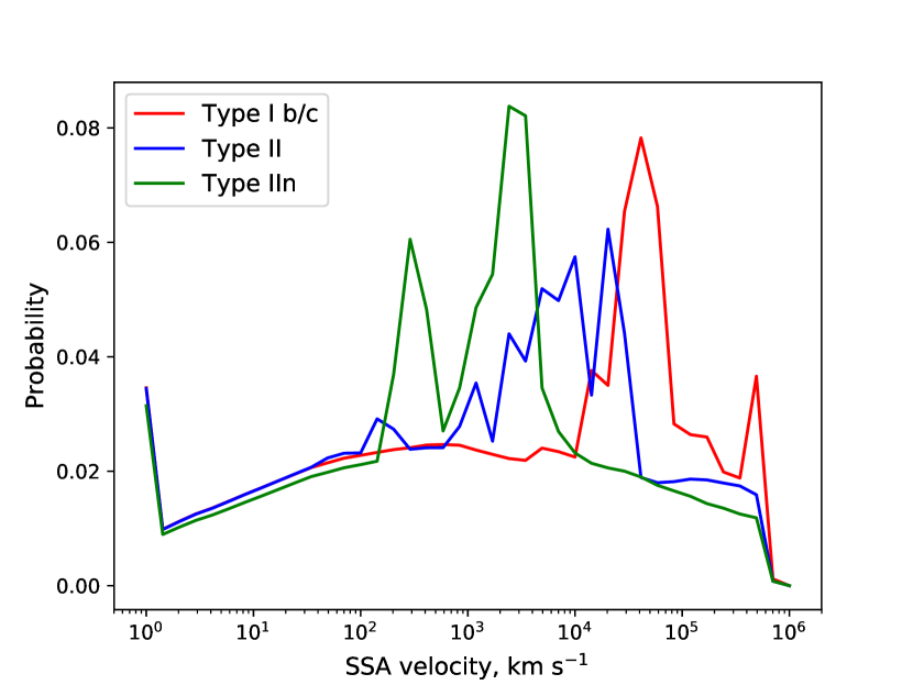
Figure 14: The normalized likelihood of different values of the SSA velocity, $v_{\rm SSA}$, over different samples of SNe. $v_{\rm SSA}$ is the velocity calculated from $t_{\rm pk}$ and $L_{\rm pk}$ assuming that the dominant absorption mechanism is synchrotron self-absorption. The likelihood is that of all our measurements arising from SNe characterized by a particular value of $v_{\rm SSA}$. Values of $v_{\rm SSA}$ which may never occur in any actual SN can have non-zero likelihood if they are not disallowed by our flux-density measurements. Note that $v_{\rm SSA}$ is a lower limit to the shock speed. We weight each SN equally. We show $p(\mbox{$v_{\rm SSA}$})$ for SNe of Type I b/c SNe (red), II (blue), and IIn (green).

7.3 Identifying the SN Type on the Basis of the Radio Lightcurve

Can the radio emission be used to determine the Type of an SN, for example in cases where there is no optical detection? Because of the large overlap in the lightcurves of different SN types, the radio lightcurve for any particular SN generally does not reliably indicate the SN type.

There are two exceptions where the radio lightcurve nevertheless can give a fairly reliable indication of the SN Type. First, a 8.4-GHz spectral luminosity $L_{\rm 8.4GHz}>10^{28}$ erg s^-1 Hz^-1 in the first month seems to occur only for Type I b/c SNe. Such high, early luminosities therefore strongly suggest a Type I b/c SN. In general, very high radio luminosities of $L_{\rm 8.4GHz}>10^{28.5}$ erg s^-1 Hz^-1 seem to occur predominantly for Type I b/c SNe regardless of age. Second, a very high luminosity at late times with $\mbox{$L_{\rm pk}$}>10^{27}$ erg s^-1 Hz^-1 at $\mbox{$t_{\rm pk}$}>1000$ d, strongly suggests a Type IIn supernova.

Third, a high value of $\mbox{$v_{\rm SSA}$}\ >30,000$ km s^-1 (see Section 7.2) suggests that the SN is much more likely to be of Type I b/c, while values of $\mbox{$v_{\rm SSA}$}\ <10,000$ km s^-1 are more likely in Type II SNe.

In our database, there are five SNe of which no optical spectrum was obtained, and of which therefore the SN Type (I or II) is unknown: SNe 1982aa, 2000ft, 2008iz, and 2010P and Spirits 16tn. Can the Type be determined from radio observations alone on the basis of our distributions of $t_{\rm pk}$ and $L_{\rm pk}$? We show the radio lightcurves of these SNe in comparison to the remainder of the SNe in our sample in Figure 15.

SN 1982aa in NGC 6052 was detected in the radio and reached a very late and high peak (Yin, 1994). Although the explosion date is uncertain, the values of $t_{\rm pk}$ and $L_{\rm pk}$ are fairly well determined at $\sim 10^{2.5}$ d and $\sim 10^{29.0}$ erg s^-1 Hz^-1, respectively. These values of $t_{\rm pk}$ and $L_{\rm pk}$ strongly suggest a Type IIn (Figures 5, 13), although the SN is exceptional regardless of Type.

SN 2000ft in NGC 7469 was detected only after the radio peak (Alberdi et al., 2006), and the explosion time is again uncertain. Although it was optically detected (Colina et al., 2007), no spectrum was obtained. The values of $t_{\rm pk}$ and $L_{\rm pk}$ are fairly well determined at $\sim\!10^{2.0}$ d and $\sim 10^{28.1}$ erg s^-1 Hz^-1, respectively. It is quite luminous compared to the majority of SNe, but the lightcurve and the values of $t_{\rm pk}$ and $L_{\rm pk}$ are equally compatible with either Type I b/c or II, so its SN Type remains unknown.

SN 2008iz was detected in the radio in M82, and was never detected optically despite the close distance (3.8 Mpc), presumably because of very strong optical extinction. It has a very unusual radio lightcurve (Marchili et al., 2010; Brunthaler et al., 2010). The values of $t_{\rm pk}$ and $L_{\rm pk}$ are fairly well determined at $\sim\!10^{1.8}$ d and $\sim\!10^{27.3}$ erg s^-1 Hz^-1, respectively. It showed both an unusually slow rise and a relatively shallow decay, and seems to be showing a late-time rise after $t\simeq 1000$ d. Although a Type II has been suggested, the radio lightcurve is equally compatible with either Type I b/c or II, although $L_{\rm pk}$ was higher than the average for either Type. Its SN Type therefore also remains unknown.

SN 2010P, in Arp 299, was discovered in the infrared and subsequently detected in the radio (Kankare et al., 2014; Romero-Cañizales et al., 2014, and references therein). Infrared observations and an optical spectrum were obtained by Kankare et al. (2014). The spectrum had relatively low signal-to-noise ratio due to the high extinction, and was compatible with an SN of either Type Ib or a IIb. In this case the peak of the radio lightcurve is not well determined, and the first measurement occurred only at $t=523$ d, so a wide range of $t_{\rm pk}$ and $L_{\rm pk}$ are compatible with the measurements. The likely values of $\log_{10}(\mbox{$t_{\rm pk}$})$ are between 1.2 and 2.5 and those of $\log_{10}(\mbox{$L_{\rm pk}$})$ between 27 and 29, with the higher values of $L_{\rm pk}$ occurring in conjunction with earlier values of $t_{\rm pk}$. While Kankare et al. (2014) suggest that the radio evolution precludes a Type Ib, we find (see Figure 15) that, when compared to our broad sample, SN 2010P’s radio evolution is not inconsistent with that seen in some Type I b/c’s. It is, however, more luminous than the mean of any of our SN Types. Although the optical spectrum rules out a normal Type II, whether SN 2010P was of Type Ib or IIb must remain uncertain.

Spirits 16tn was a heavily obscured SN, detected in the infrared, for which spectroscopic classification was not possible (Jencson et al., 2018). Fairly low limits of $L_{\rm 6GHz}\lesssim 10^{24.3}$ erg s^-1 Hz^-1 were placed on the radio luminosity (Jencson et al., 2018). However, as can be seen from Figs. 13 and 15, such low values can occur for either Type I b/c or Type II SNe, therefore its SN Type must also remain uncertain.

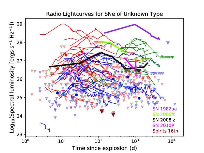
Figure 15: The radio lightcurves or limits of five SNe which were not spectroscopically identified, compared to those of the spectroscopically confirmed SNe of Types I b/c (red) and II (blue) and IIn (green) in our sample. SNe 1982aa, 2000ft, 2008iz, 2010P and Spirits 16tn are highlighted in violet, light green, black, magenta and maroon, respectively. Spirits 16tn was not detected, but two fairly low limits were obtained, shown as larger maroon triangles between $t=100$ and 300 d. SN 1982aa is most likely of Type IIn. For SNe 2000ft, 2008iz and 2010P, and Spirits 16tn, the radio lightcurves do not permit a conclusive identification of the SN Type.

7.4 Determining Mass Loss Rates from Radio Emission

From the distribution of $t_{\rm pk}$ and $L_{\rm pk}$, a distribution of mass-loss rates, $\dot{M}$, for the progenitors can be estimated. For both SN Type I b/c and Type II the mean values of $\dot{M}$ are low compared to the published values for well-studied SNe. This is because the well-studied SNe tend to be substantially brighter than the average, and thus tend to have denser CSM to produce the stronger radio emission than the average. We found that the average value of $\log_{10}(\mbox{$\dot{M}$})$ for a Type I b/c SNe was $-5.6\pm 1.1$ (in M$\odot$ yr^-1; assuming $v_{\rm wind}$ = 1000 km s^-1), while the equivalent value for Type II’s (excluding IIn’s) was lower at $-6.8\pm 1.4$ (assuming $v_{\rm wind}$ = 10 km s^-1). However, we caution against over-interpreting this difference, since our values of $\dot{M}$ rely on a number of assumptions (see Section 6), and there may be systematic biases dependent on the type of the SN since the mass-loss rates are calculated differently for Type I b/c’s than for Type II’s. Also, as with $t_{\rm pk}$ and $L_{\rm pk}$, the range of values of $\dot{M}$ is quite large, with the standard deviations of $\log_{10}(\mbox{$\dot{M}$})$ over our sample being 1.1 and 1.4, respectively, so here also there is considerable overlap between Type I b/c’s and Type II’s.

To indicate the uncertainty in estimating the mass loss rate we give as an example SN 1993J, whose 8.4-GHz lightcurve we showed in Figure 1. Despite being one of the most intensely studied SNe with extensive, multi-frequency radio lightcurves as well as X-ray data, estimating $\dot{M}$ seems to be far from straightforward, and various authors have reported a considerable range of $\log_{10}(\mbox{$\dot{M}$})$ for its progenitor. In $\log_{10}$($\dot{M}$/M$\odot$ yr^-1), for $v_{\rm wind}$= 10 km s^-1, Weiler et al. (2007) reports values between $-6.3$ and $-5.2$, Björnsson (2015) reports $-5.0$, Weiler et al. (2002) report $-4.6$, and Fransson & Björnsson (1998) report $-4.3$. We found that the distribution of $\log_{10}(\mbox{$\dot{M}$})$ for all Type II SNe excluding Type IIn’s had a mean of $-6.8$ and standard deviation of 1.4. The cited values for SN 1993J, are higher than the mean of the distribution, although not outlandish, with, for example, $\sim$4% of SNe having $\dot{M}$ higher than even the highest of the values reported for SN 1993J ($\log_{10}(\mbox{$\dot{M}$})=-4.3)$. Since SN 1993J was exceptionally radio luminous, it is not surprising that it has a denser CSM, and thus that its progenitor had a higher $\dot{M}$ than the population average.

In the standard self-similar model of an SN, the rise of the radio lightcurve to $L_{\rm pk}$ is relatively rapid, regardless of whether FFA or SSA is the dominant absorption mechanism, and is followed by a slower decay. For external FFA by a uniform wind medium, with density $\propto r^{-2}$, the optical depth, $\tau$, is expected to decay with time as $\tau\propto t^{-\delta}$ with $\delta\simeq 2.5$ (see, e.g. Weiler et al., 2002). Inspection of Figure 2 shows that such steeply rising lightcurves are not common. We used $\delta=1$, which is more representative, for our lightcurve model. To check the dependence of our results on the assumed $\delta=1$, we tried a model with $\delta=2.5$ but obtained a much lower likelihood than with $\delta=1$. We note that $\delta=0.9$ produces a marginally higher likelihood than $\delta=1$, but the difference is small, and our results should not be compromised by our use of $\delta=1$.

If the rising part of the lightcurve (in a self-similar model) were due to SSA within the emitting region, rather than FFA, then the rising part would be expected to be a power-law, $L_{\nu}\propto t^{a}$, rather than exponential as seen with FFA. In the case of pure SSA, values of $a\sim 2.1$ are expected (Chevalier, 1998). This expected value again is much steeper than the majority of the observed lightcurves in Figure 2. We fitted our data with SSA-like model lightcurves with a power-law, rather than an exponential rise. We found that a fit with $a=2.1$ produces much lower likelihood than our standard model (exponential rise with $\delta=1$). Smaller values of $a$ produced higher likelihoods, although over the whole sample, an exponential rise with $\tau\propto t^{-1}$ produced a somewhat higher likelihood than a power-law rise for any value of $a$.

Weiler et al. (2002) also found that absorption by a uniform wind medium cannot fit the rising portions of many SN radio lightcurves. They appeal to geometrical effects from a clumpy absorbing medium to flatten the rise and produce a better fit to the rising part of the lightcurves. Björnsson & Keshavarzi (2017) model the effect of an inhomogeneous synchrotron-emitting region in SSA-dominated SNe, and find the effect is to flatten the part of the SED below the peak, which would also tend to make the rise in the lightcurve less steep.

From our much larger collection of measurements we can conclude that the slowly rising lightcurves are a fairly general phenomenon and that therefore some form of geometrical effect, such as clumpiness in the CSM or inhomogeneity in the synchrotron-emitting region, are common.

7.5 Structure of a Comprehensive Radio SN Observing Program

Our sample is of necessity heterogeneous and incomplete, with only a fraction of SNe being observed at all in the radio, and even if observed, often with very sparse sampling in time. While a census of southern SNe is one of the goals of the Variables and Slow Transients survey (VAST; Murphy et al., 2013), to be conducted with the Australian Square Kilometre Array Pathfinder at 1.4 GHz, as well as of the ThunderKAT transients programme underway at MeerKAT (Fender et al., 2016), a systematic multi-frequency program of observing SNe in the radio would be desirable to obtain a clearer picture of the radio SN luminosity-risetime function. What would such a program entail?

We found the mean $\log_{10}(\mbox{$L_{\rm pk}$})$ for our sample of all Types of core-collapse SNe was 25.5 (in erg s^-1 Hz^-1) with a standard deviation of 1.6 (Table 4). This mean $\log_{10}(\mbox{$L_{\rm pk}$})$ corresponds to a flux density of 30 $\mu$Jy at 30 Mpc.

To achieve a $5\sigma$ detection of 30 $\mu$Jy requires $\sim$30 min at 10 GHz or $\sim$3 h at 1.5 GHz with the VLA, $\sim$4 h at 10 GHz or $\sim$7 h at 2 GHz with ATCA, and $\sim$2 h at 1.3 GHz with MeerKAT. Note that this is only the mean $\log_{10}(\mbox{$L_{\rm pk}$})$, so at this sensitivity level $\sim$50% of SNe would remain undetected. On the Transient Name Server, the rate of classified SNe with $D<30$ Mpc is $\sim$16 yr^-1 over the whole sky. Observations to fully sample the luminosity distribution of radio SNe will therefore be challenging with current instrumentation.

Given the wide range of $t_{\rm pk}$ that we have found, with the 1-$\sigma$ range being from 7 d to 1 yr, an observing program with at least 7 logarithmically-spaced observations of each SN starting after about one week and extending to at least $t=1$ yr would be required to get reasonably complete sampling and provide accurate constraints on $t_{\rm pk}$ and $L_{\rm pk}$. Obviously such a program will miss the $\sim$17% of SNe with $\mbox{$t_{\rm pk}$}<$ 1 week but observations on a shorter timescale would be hard to schedule.

A systematic program to provide more robust statistics with a more complete sample than we have been able to do with the existing ad-hoc sample would therefore be a challenging and long-term project with current instrumentation, but would certainly be an important project with the Square Kilometre Array, whose sensitivity will greatly surpass that of current instruments (Perez-Torres et al., 2015a). Notwithstanding the difficulty of obtaining a complete sample with current instrumentation, it is still well worthwhile to observe nearby or unusual SNe on a case-by-case basis, and we encourage observers to publish non-detections.

8 Conclusion

We examined a large number of radio flux density measurements for 294 SNe at between 5 and 10 GHz. We parameterize the radio lightcurves by a simple model consisting of an optically-thick rise over time $t_{\rm pk}$ from the explosion, to a maximum value of the spectral luminosity, $L_{\rm pk}$, followed by a power-law decay with $L_{\nu}\propto t^{-1.5}$. We concentrate here only on the part of the lightcurve near the initial peak, and disregard any late-time rises in flux density, such as observed in, e.g., SN 1987A.

We find that both $t_{\rm pk}$ and $L_{\rm pk}$ vary over large ranges. In the case of $t_{\rm pk}$, some SNe (such as SN 1987A) had $t_{\rm pk}$ of a couple of days or even less, while others (such as SN 1986J) do not reach the peak until $\mbox{$t_{\rm pk}$}\gtrsim 1000$ d.

The range in $L_{\rm pk}$ is even larger: SN 1987A reached $L_{\rm pk}$ of only $\sim\!10^{23.6}$ erg s^-1 Hz^-1, while that of SN 1998bw was $\sim\!10^{29}$ erg s^-1 Hz^-1.

1. We find that, over our sample of SNe, lognormal distributions of $t_{\rm pk}$ and $L_{\rm pk}$ provide a reasonable fit to the measurements, including the many upper limits.

2. Many SNe in our sample have low values of $L_{\rm pk}$. At 8.4 GHz, 50% of all SNe have $\mbox{$L_{\rm pk}$}<10^{25.5}$ erg s^-1 Hz^-1 or flux densities $<30\;\mu$Jy at $D=30$ Mpc.

3. The median value of $L_{\rm pk}$ is $\sim$30 times lower than that obtained if one does not consider the many upper limits in addition to the detections.

4. For Type I b/c SNe at $D<100$ Mpc, the mean value and standard deviation of $t_{\rm pk}$ were $10^{1.1\pm 0.5}$ d, and those of $L_{\rm pk}$ were $10^{25.4\pm 1.7}$ erg s^-1 Hz^-1. Type I b/c SNe are characterized by more rapid rises than are Type II’s, but they reach similar values of $L_{\rm pk}$.

5. For Type II SNe, at $D<100$ Mpc and excluding Type IIn’s, the mean value and standard deviation of $t_{\rm pk}$ were $10^{1.6\pm 1.0}$ d, and those of $L_{\rm pk}$ were $10^{25.3\pm 1.3}$ erg s^-1 Hz^-1.

6. Type IIn SNe are characterized by long risetimes, $10^{3.1\pm 0.7}$ d but high values of $L_{\rm pk}$ of $10^{26.5\pm 1.1}$ erg s^-1 Hz^-1.

7. Type IIb SNe seem to be characterized by considerably higher $L_{\rm pk}$ than the remainder of the Type II’s of $10^{26.8\pm 0.5}$ erg s^-1 Hz^-1, and also a narrower range of $L_{\rm pk}$ than other Types. However, our sample contained only 19 Type IIb SNe, so this distribution is somewhat uncertain.

8. In general, given the wide distributions, the values of $t_{\rm pk}$ and $L_{\rm pk}$ for any particular SN do not reliably indicate whether the SN is of Type I b/c or II.

9. The exception to item 8. above is that $L_{\nu}>10^{28}$ erg s^-1 Hz^-1 in the first month strongly suggests a Type I b/c SN.

10. From the distribution of $t_{\rm pk}$ and $L_{\rm pk}$ values we estimated also the distribution of mass-loss rates, $\dot{M}$. We found that for Type I b/c SNe, $\mbox{$\dot{M}$}=10^{-5.6\pm 1.1}$ M$\odot$ yr^-1, while for Type II SNe excluding Type IIn’s, $\mbox{$\dot{M}$}=10^{-6.8\pm 1.4}$ M$\odot$ yr^-1, for assumed $v_{\rm wind}$ of 1000 km s^-1 and 10 km s^-1, respectively. We caution, however, that the determination of $\dot{M}$ from $t_{\rm pk}$ and $L_{\rm pk}$ is very imprecise, and possibly subject to biases that could be dependent on the SN Type.

11. We find that the rising part of the lightcurves is in most cases too shallow to be described either by synchrotron self-absorption (SSA) or free-free absorption in a uniform medium. This relative flatness suggests that geometrical effects, such as a clumpy CSM or non-spherically symmetric structure in the ejecta or the CSM, are likely common among SNe.

References

- Alberdi et al. (2006) Alberdi, A., Colina, L., Torrelles, J. M., et al. 2006, ApJ, 638, 938
- Argo (2007) Argo, M. 2007, in From Planets to Dark Energy: the Modern Radio Universe, 82
- Argo (2014) Argo, M. 2014, e-MERLIN data reduction pipeline, ascl:1407.017
- Argo et al. (2017a) Argo, M., Torres, M. P., Beswick, R., & Wrigley, N. 2017a, The Astronomer’s Telegram, 10421
- Argo et al. (2017b) —. 2017b, The Astronomer’s Telegram, 10472
- Argo et al. (2007) Argo, M. K., Beswick, R. J., Muxlow, T. W. B., & Pedlar, A. 2007, The Astronomer’s Telegram, 1084, 1
- Argo et al. (2008) Argo, M. K., Beswick, R. J., Muxlow, T. W. B., et al. 2008, The Astronomer’s Telegram, 1469, 1
- Argo et al. (2016) Argo, M. K., Romero-Canizales, C., Beswick, R., & Prieto, J. L. 2016, The Astronomer’s Telegram, 9147, 1
- Associated Universities (1999) Associated Universities, I. 1999, AIPS: Astronomical Image Processing System, ascl:9911.003
- Bannister et al. (2017) Bannister, K., Corsi, A., & Sand, D. 2017, The Astronomer’s Telegram, 10660, 1
- Bartel & Bietenholz (2008) Bartel, N., & Bietenholz, M. F. 2008, ApJ, 682, 1065
- Bartel et al. (2007) Bartel, N., Bietenholz, M. F., Rupen, M. P., & Dwarkadas, V. V. 2007, ApJ, 668, 924
- Bartel et al. (2002) Bartel, N., Bietenholz, M. F., Rupen, M. P., et al. 2002, ApJ, 581, 404
- Bauer et al. (2008) Bauer, F. E., Dwarkadas, V. V., Brandt, W. N., et al. 2008, ApJ, 688, 1210
- Berger et al. (2002) Berger, E., Kulkarni, S. R., & Chevalier, R. A. 2002, ApJ, 577, L5
- Berger et al. (2003) Berger, E., Kulkarni, S. R., Frail, D. A., & Soderberg, A. M. 2003, ApJ, 599, 408
- Beswick et al. (2005) Beswick, R. J., Fenech, D., Thrall, H., et al. 2005, IAU Circ., 8572, 1
- Beswick et al. (2004) Beswick, R. J., Muxlow, T. W. B., Argo, M. K., & Pedlar, A. 2004, IAU Circ., 8332, 2
- Bietenholz (2014) Bietenholz, M. 2014, in 12th European VLBI Network Symposium and Users Meeting (2014), published by SISSA, Trieste, ed. A. Tarchi, M. Giroletti, & L. Feretti, 51
- Bietenholz & Bartel (2007a) Bietenholz, M., & Bartel, N. 2007a, The Astronomer’s Telegram, 1254, 1
- Bietenholz & Bartel (2008a) —. 2008a, The Astronomer’s Telegram, 1525, 1
- Bietenholz & Bartel (2008b) —. 2008b, The Astronomer’s Telegram, 1657, 1
- Bietenholz & Bartel (2014) —. 2014, The Astronomer’s Telegram, 6429, 1
- Bietenholz & Bartel (2005) Bietenholz, M. F., & Bartel, N. 2005, ApJ, 625, L99
- Bietenholz & Bartel (2007b) —. 2007b, ApJ, 665, L47
- Bietenholz & Bartel (2017a) —. 2017a, ApJ, 839, 10
- Bietenholz & Bartel (2017b) —. 2017b, ApJ, 851, 7
- Bietenholz et al. (2002) Bietenholz, M. F., Bartel, N., & Rupen, M. P. 2002, ApJ, 581, 1132
- Bietenholz et al. (2010a) —. 2010a, ApJ, 712, 1057
- Bietenholz et al. (2014) Bietenholz, M. F., De Colle, F., Granot, J., Bartel, N., & Soderberg, A. M. 2014, MNRAS, 440, 821
- Bietenholz et al. (2018) Bietenholz, M. F., Kamble, A., Margutti, R., Milisavljevic, D., & Soderberg, A. 2018, MNRAS, 475, 1756
- Bietenholz et al. (2009) Bietenholz, M. F., Soderberg, A. M., & Bartel, N. 2009, ApJ, 694, L6
- Bietenholz et al. (2010b) Bietenholz, M. F., Soderberg, A. M., Bartel, N., et al. 2010b, ApJ, 725, 4
- Björnsson (2015) Björnsson, C. I. 2015, ApJ, 813, 43
- Björnsson & Keshavarzi (2017) Björnsson, C. I., & Keshavarzi, S. T. 2017, ApJ, 841, 12
- Bostroem et al. (2019) Bostroem, K. A., Valenti, S., Horesh, A., et al. 2019, MNRAS, 485, 5120
- Brunthaler et al. (2010) Brunthaler, A., Marti-Vidal, I., Menten, K. M., et al. 2010, in 10th European VLBI Network Symposium and EVN Users Meeting: VLBI and the New Generation of Radio Arrays, Vol. 10, 55
- Bufano et al. (2014) Bufano, F., Pignata, G., Bersten, M., et al. 2014, MNRAS, 439, 1807
- Cano et al. (2017) Cano, Z., Wang, S.-Q., Dai, Z.-G., & Wu, X.-F. 2017, Advances in Astronomy, 2017, 8929054
- Cendes et al. (2018) Cendes, Y., Gaensler, B. M., Ng, C. Y., et al. 2018, ApJ, 867, 65
- Chakraborti et al. (2013) Chakraborti, S., Ray, A., Smith, R., et al. 2013, ApJ, 774, 30
- Chakraborti et al. (2015) Chakraborti, S., Soderberg, A., Chomiuk, L., et al. 2015, ApJ, 805, 187
- Chandra et al. (2012) Chandra, P., Chevalier, R. A., Chugai, N., et al. 2012, ApJ, 755, 110
- Chandra et al. (2015) Chandra, P., Chevalier, R. A., Chugai, N., Fransson, C., & Soderberg, A. M. 2015, ApJ, 810, 32
- Chandra et al. (2019) Chandra, P., Nayana, A. J., Björnsson, C. I., et al. 2019, ApJ, 877, 79
- Chandra et al. (2002) Chandra, P., Ray, A., & Bhatnagar, S. 2002, IAU Circ., 7982, 2
- Chandra & Soderberg (2007a) Chandra, P., & Soderberg, A. 2007a, The Astronomer’s Telegram, 1182, 1
- Chandra & Soderberg (2007b) —. 2007b, The Astronomer’s Telegram, 1271, 1
- Chandra & Soderberg (2008a) —. 2008a, The Astronomer’s Telegram, 1869, 1
- Chandra & Soderberg (2008b) —. 2008b, The Astronomer’s Telegram, 1366, 1
- Chandra & Soderberg (2008c) —. 2008c, The Astronomer’s Telegram, 1359, 1
- Chandra & Soderberg (2008d) —. 2008d, The Astronomer’s Telegram, 1409, 1
- Chandra & Soderberg (2008e) —. 2008e, The Astronomer’s Telegram, 1410, 1
- Chandra & Soderberg (2009a) —. 2009a, The Astronomer’s Telegram, 1891, 1
- Chandra & Soderberg (2009b) —. 2009b, The Astronomer’s Telegram, 2070, 1
- Chandra & Soderberg (2009c) —. 2009c, The Astronomer’s Telegram, 2335, 1
- Chandra & Soderberg (2009d) —. 2009d, The Astronomer’s Telegram, 2351, 1
- Chandra & Soderberg (2009e) —. 2009e, The Astronomer’s Telegram, 2358, 1
- Chandra et al. (2010) Chandra, P., Soderberg, A., Chevalier, R., Fransson, C., & Chugai, N. 2010, The Astronomer’s Telegram, 2532, 1
- Chandra et al. (2009) Chandra, P., Stockdale, C. J., Chevalier, R. A., et al. 2009, ApJ, 690, 1839
- Chevalier (1982) Chevalier, R. A. 1982, ApJ, 259, 302
- Chevalier (1998) —. 1998, ApJ, 499, 810
- Chevalier (2007) Chevalier, R. A. 2007, in Revista Mexicana de Astronomia y Astrofisica, vol. 27, Vol. 30, Revista Mexicana de Astronomia y Astrofisica Conference Series, 41–48
- Chevalier & Fransson (2006) Chevalier, R. A., & Fransson, C. 2006, ApJ, 651, 381
- Colina et al. (2007) Colina, L., Díaz-Santos, T., Alonso-Herrero, A., et al. 2007, A&A, 467, 559
- Corsi et al. (2018) Corsi, A., Ho, A., & Kulkarni, S. 2018, The Astronomer’s Telegram, 11295, 1
- Corsi et al. (2011) Corsi, A., Ofek, E. O., Frail, D. A., et al. 2011, ApJ, 741, 76
- Corsi et al. (2012) Corsi, A., Ofek, E. O., Gal-Yam, A., et al. 2012, ApJ, 747, L5
- de Jaeger et al. (2019) de Jaeger, T., Zheng, W., Stahl, B. E., et al. 2019, MNRAS, 490, 2799
- de Witt et al. (2016) de Witt, A., Bietenholz, M. F., Kamble, A., et al. 2016, MNRAS, 455, 511
- Dobie et al. (2018a) Dobie, D., Ravi, V., Ho, A., Kasliwal, M., & Murphy, T. 2018a, The Astronomer’s Telegram, 11795
- Dobie et al. (2018b) Dobie, D., Ravi, V., Ho, A., Kasliwal, M., & Murphy, T. 2018b, The Astronomer’s Telegram, 11818
- Dobie et al. (2018c) Dobie, D., Ravi, V., Ho, A., Kasliwal, M., & Murphy, T. 2018c, The Astronomer’s Telegram, 11862
- Drout et al. (2013) Drout, M. R., Soderberg, A. M., Mazzali, P. A., et al. 2013, ApJ, 774, 58
- Drout et al. (2016) Drout, M. R., Milisavljevic, D., Parrent, J., et al. 2016, ApJ, 821, 57
- Dwarkadas et al. (2016) Dwarkadas, V. V., Romero-Cañizales, C., Reddy, R., & Bauer, F. E. 2016, MNRAS, 462, 1101
- Fender et al. (2016) Fender, R., Woudt, P. A., Corbel, S., et al. 2016, in MeerKAT Science: On the Pathway to the SKA, 13
- Fransson & Björnsson (1998) Fransson, C., & Björnsson, C.-I. 1998, ApJ, 509, 861
- Hancock & Horesh (2016) Hancock, P., & Horesh, A. 2016, The Astronomer’s Telegram, 8504, 1
- Ho et al. (2019) Ho, A. Y. Q., Goldstein, D. A., Schulze, S., et al. 2019, ApJ, 887, 169
- Ho et al. (2020a) Ho, A. Y. Q., Kulkarni, S. R., Perley, D. A., et al. 2020a, ApJ, 902, 86
- Ho et al. (2020b) Ho, A. Y. Q., Corsi, A., Cenko, S. B., et al. 2020b, ApJ, 893, 132
- Horesh et al. (2013a) Horesh, A., Cao, Y., Mooley, K., & Carpenter, J. 2013a, The Astronomer’s Telegram, 5198, 1
- Horesh et al. (2011) Horesh, A., Kasliwal, M., Carpenter, J., et al. 2011, The Astronomer’s Telegram, 3512, 1
- Horesh et al. (2013b) Horesh, A., Stockdale, C., Fox, D. B., et al. 2013b, MNRAS, 436, 1258
- Horesh et al. (2013c) Horesh, A., Kulkarni, S. R., Corsi, A., et al. 2013c, ApJ, 778, 63
- Horesh et al. (2020) Horesh, A., Sfaradi, I., Ergon, M., et al. 2020, ApJ, 903, 132
- International Consortium Of Scientists (2011) International Consortium Of Scientists. 2011, CASA: Common Astronomy Software Applications, ascl:1107.013
- Jacobson-Galán et al. (2020) Jacobson-Galán, W. V., Margutti, R., Kilpatrick, C. D., et al. 2020, ApJ, 898, 166
- Jencson et al. (2018) Jencson, J. E., Kasliwal, M. M., Adams, S. M., et al. 2018, ApJ, 863, 20
- Kamble et al. (2015) Kamble, A., Margutti, R., Milisavljevic, D., Soderberg, A., & Parrent, J. 2015, The Astronomer’s Telegram, 7845, 1
- Kamble & Soderberg (2013) Kamble, A., & Soderberg, A. 2013, The Astronomer’s Telegram, 5154, 1
- Kamble et al. (2014a) Kamble, A., Soderberg, A., Margutti, R., Parrent, J., & Milisavljevic, D. 2014a, The Astronomer’s Telegram, 6724
- Kamble et al. (2014b) Kamble, A., Soderberg, A. M., Chomiuk, L., et al. 2014b, ApJ, 797, 2
- Kamble et al. (2016a) Kamble, A., Margutti, R., Soderberg, A. M., et al. 2016a, ApJ, 818, 111
- Kamble et al. (2016b) Kamble, A., Margutti, R., Alexander, K., et al. 2016b, The Astronomer’s Telegram, 8911
- Kankare et al. (2014) Kankare, E., Fraser, M., Ryder, S., et al. 2014, A&A, 572, A75
- Kasliwal et al. (2010a) Kasliwal, M., Frail, D., Quimby, R., et al. 2010a, The Astronomer’s Telegram, 3090, 1
- Kasliwal et al. (2010b) Kasliwal, M., Kulkarni, S., Arcavi, I., et al. 2010b, The Astronomer’s Telegram, 2864, 1
- Kasliwal et al. (2010c) Kasliwal, M. M., Frail, D., Quimby, R., et al. 2010c, The Astronomer’s Telegram, 3093, 1
- Kelley et al. (2006) Kelley, M. T., Stockdale, C. J., Sramek, R. A., et al. 2006, Central Bureau Electronic Telegrams, 495, 1
- Kimani et al. (2016) Kimani, N., Sendlinger, K., Brunthaler, A., et al. 2016, A&A, 593, A18
- Krauss et al. (2012) Krauss, M. I., Soderberg, A. M., Chomiuk, L., et al. 2012, ApJ, 750, L40
- Kulkarni et al. (1998) Kulkarni, S. R., Frail, D. A., Wieringa, M. H., et al. 1998, Nature, 395, 663
- Kundu & Ryder (2019) Kundu, E., & Ryder, S. 2019, The Astronomer’s Telegram, 13040, 1
- Kundu et al. (2020a) Kundu, E., Ryder, S. D., Filipovic, M. D., et al. 2020a, The Astronomer’s Telegram, 13477, 1
- Kundu et al. (2020b) —. 2020b, The Astronomer’s Telegram, 13805, 1
- Lacey et al. (1999) Lacey, C. K., Van Dyk, S. D., Weiler, K. W., et al. 1999, IAU Circ., 7336, 2
- Lacey et al. (1998) Lacey, C. K., Weiler, K. W., Sramek, R. A., & van Dyk, S. D. 1998, IAU Circ., 7068, 2
- Li et al. (2011) Li, W., Leaman, J., Chornock, R., et al. 2011, MNRAS, 412, 1441
- Lien et al. (2011) Lien, A., Chakraborty, N., Fields, B. D., & Kemball, A. 2011, ApJ, 740, 23
- Lundqvist et al. (2020) Lundqvist, P., Kundu, E., Pérez-Torres, M. A., et al. 2020, ApJ, 890, 159
- Marchili et al. (2010) Marchili, N., Martí-Vidal, I., Brunthaler, A., et al. 2010, A&A, 509, A47
- Margutti et al. (2013) Margutti, R., Soderberg, A. M., Wieringa, M. H., et al. 2013, ApJ, 778, 18
- Margutti et al. (2014) Margutti, R., Milisavljevic, D., Soderberg, A. M., et al. 2014, ApJ, 780, 21
- Margutti et al. (2017) Margutti, R., Kamble, A., Milisavljevic, D., et al. 2017, ApJ, 835, 140
- Margutti et al. (2019) Margutti, R., Metzger, B. D., Chornock, R., et al. 2019, ApJ, 872, 18
- Marongiu et al. (2019) Marongiu, M., Guidorzi, C., Margutti, R., et al. 2019, ApJ, 879, 89
- Martí-Vidal et al. (2011) Martí-Vidal, I., Marcaide, J. M., Alberdi, A., et al. 2011, A&A, 526, A142
- Martí-Vidal et al. (2007) —. 2007, A&A, 470, 1071
- Milisavljevic et al. (2013) Milisavljevic, D., Margutti, R., Soderberg, A. M., et al. 2013, ApJ, 767, 71
- Milisavljevic et al. (2015) Milisavljevic, D., Margutti, R., Kamble, A., et al. 2015, ApJ, 815, 120
- Milisavljevic et al. (2017) Milisavljevic, D., Patnaude, D. J., Raymond, J. C., et al. 2017, ApJ, 846, 50
- Montes et al. (1997) Montes, M. J., Van Dyk, S. D., Weiler, K. W., Sramek, R. A., & Panagia, N. 1997, ApJ, 482, L61
- Montes et al. (1998) —. 1998, ApJ, 506, 874
- Montes et al. (2000) Montes, M. J., Weiler, K. W., Van Dyk, S. D., et al. 2000, ApJ, 532, 1124
- Mould et al. (2000) Mould, J. R., Huchra, J. P., Freedman, W. L., et al. 2000, ApJ, 529, 786
- Murphy et al. (2013) Murphy, T., Chatterjee, S., Kaplan, D. L., et al. 2013, PASA, 30, 6
- Nayana et al. (2018) Nayana, A. J., Chandra, P., & Ray, A. K. 2018, ApJ, 863, 163
- Palliyaguru et al. (2019) Palliyaguru, N. T., Corsi, A., Frail, D. A., et al. 2019, ApJ, 872, 201
- Panagia et al. (1986) Panagia, N., Sramek, R. A., & Weiler, K. W. 1986, ApJ, 300, L55
- Perez-Torres et al. (2015a) Perez-Torres, M., Alberdi, A., Beswick, R. J., et al. 2015a, in Advancing Astrophysics with the Square Kilometre Array (AASKA14), 60
- Perez-Torres et al. (2015b) Perez-Torres, M., Argo, M., Martí-Vidal, I., et al. 2015b, The Astronomer’s Telegram, 8452, 1
- Pérez-Torres et al. (2009) Pérez-Torres, M. A., Alberdi, A., Colina, L., et al. 2009, MNRAS, 399, 1641
- Pihlström et al. (2007) Pihlström, Y. M., Taylor, G. B., Granot, J., & Doeleman, S. 2007, ApJ, 664, 411
- Planck Collaboration et al. (2020) Planck Collaboration, Aghanim, N., Akrami, Y., et al. 2020, A&A, 641, A6
- Romero-Cañizales et al. (2014) Romero-Cañizales, C., Herrero-Illana, R., Pérez-Torres, M. A., et al. 2014, MNRAS, 440, 1067
- Roming et al. (2009) Roming, P. W. A., Pritchard, T. A., Brown, P. J., et al. 2009, ApJ, 704, L118
- Roy et al. (2013) Roy, R., Kumar, B., Maund, J. R., et al. 2013, MNRAS, 434, 2032
- Ryder et al. (2019a) Ryder, S., Kundu, E., Marnoch, L., Chomiuk, L., & Sarbadhicary, S. 2019a, The Astronomer’s Telegram, 12820, 1
- Ryder et al. (2010a) Ryder, S., Covarrubias, R., Amy, S., et al. 2010a, Central Bureau Electronic Telegrams, 2242, 1
- Ryder et al. (2010b) Ryder, S. D., Amy, S. W., Stockdale, C. J., et al. 2010b, The Astronomer’s Telegram, 2450, 1
- Ryder et al. (2011a) —. 2011a, The Astronomer’s Telegram, 3370, 1
- Ryder et al. (2015) Ryder, S. D., Kool, E., Stockdale, C. J., & Kotak, R. 2015, The Astronomer’s Telegram, 7762, 1
- Ryder et al. (2019b) Ryder, S. D., Kool, E. C., Filipovic, M., et al. 2019b, The Astronomer’s Telegram, 12373
- Ryder et al. (2016a) Ryder, S. D., Kool, E. C., Stockdale, C. J., & Kotak, R. 2016a, The Astronomer’s Telegram, 8836, 1
- Ryder et al. (2016b) Ryder, S. D., Kool, E. C., Stockdale, C. J., et al. 2016b, The Astronomer’s Telegram, 9475
- Ryder et al. (2017) —. 2017, The Astronomer’s Telegram, 10147, 1
- Ryder et al. (2016c) Ryder, S. D., Kool, E. C., Stockdale, C. J., Romero-Canizales, C., & Kotak, R. 2016c, The Astronomer’s Telegram, 8815, 1
- Ryder et al. (2020) Ryder, S. D., Kundu, E., Filipovic, M. D., et al. 2020, The Astronomer’s Telegram, 13642, 1
- Ryder et al. (2019c) Ryder, S. D., Kundu, E., Velovic, V., et al. 2019c, The Astronomer’s Telegram, 13136, 1
- Ryder et al. (2004) Ryder, S. D., Sadler, E. M., Subrahmanyan, R., et al. 2004, MNRAS, 349, 1093
- Ryder et al. (2011b) Ryder, S. D., Stockdale, C. J., Immler, S., et al. 2011b, The Astronomer’s Telegram, 3764, 1
- Salas et al. (2013) Salas, P., Bauer, F. E., Stockdale, C., & Prieto, J. L. 2013, MNRAS, 428, 1207
- Sanders et al. (2012) Sanders, N. E., Soderberg, A. M., Valenti, S., et al. 2012, ApJ, 756, 184
- Sault et al. (1995) Sault, R. J., Teuben, P. J., & Wright, M. C. H. 1995, in Astronomical Society of the Pacific Conference Series, Vol. 77, Astronomical Data Analysis Software and Systems IV, ed. R. A. Shaw, H. E. Payne, & J. J. E. Hayes, 433
- Schinzel et al. (2009) Schinzel, F. K., Taylor, G. B., Stockdale, C. J., Granot, J., & Ramirez-Ruiz, E. 2009, ApJ, 691, 1380
- Shivvers et al. (2017) Shivvers, I., Zheng, W., Van Dyk, S. D., et al. 2017, MNRAS, 471, 4381
- Smith et al. (2011) Smith, N., Li, W., Filippenko, A. V., & Chornock, R. 2011, MNRAS, 412, 1522
- Smith et al. (2012) Smith, N., Cenko, S. B., Butler, N., et al. 2012, MNRAS, 420, 1135
- Smith et al. (2017) Smith, N., Kilpatrick, C. D., Mauerhan, J. C., et al. 2017, MNRAS, 466, 3021
- Soderberg (2007) Soderberg, A. 2007, PhD thesis, California Institute of Technology
- Soderberg (2008) —. 2008, The Astronomer’s Telegram, 1811, 1
- Soderberg & Chandra (2008) Soderberg, A., & Chandra, P. 2008, The Astronomer’s Telegram, 1470, 1
- Soderberg et al. (2010) Soderberg, A. M., Brunthaler, A., Nakar, E., Chevalier, R. A., & Bietenholz, M. F. 2010, ApJ, 725, 922
- Soderberg et al. (2006a) Soderberg, A. M., Chevalier, R. A., Kulkarni, S. R., & Frail, D. A. 2006a, ApJ, 651, 1005
- Soderberg et al. (2005) Soderberg, A. M., Kulkarni, S. R., Berger, E., et al. 2005, ApJ, 621, 908
- Soderberg et al. (2006b) Soderberg, A. M., Nakar, E., Berger, E., & Kulkarni, S. R. 2006b, ApJ, 638, 930
- Soderberg et al. (2006c) Soderberg, A. M., Kulkarni, S. R., Nakar, E., et al. 2006c, Nature, 442, 1014
- Soderberg et al. (2008) Soderberg, A. M., Berger, E., Page, K. L., et al. 2008, Nature, 453, 469
- Soderberg et al. (2012) Soderberg, A. M., Margutti, R., Zauderer, B. A., et al. 2012, ApJ, 752, 78
- Sramek et al. (1984) Sramek, R. A., Panagia, N., & Weiler, K. W. 1984, ApJ, 285, L59
- Stockdale et al. (2005) Stockdale, C. J., Kelley, M., van Dyk, S. D., et al. 2005, IAU Circ., 8603, 2
- Stockdale et al. (2007) Stockdale, C. J., Kelley, M. T., Weiler, K. W., et al. 2007, in American Institute of Physics Conference Series, Vol. 937, Supernova 1987A: 20 Years After: Supernovae and Gamma-Ray Bursters, ed. S. Immler, K. Weiler, & R. McCray, 264–268
- Stockdale et al. (2003) Stockdale, C. J., Sramek, R. A., Van Dyk, S. D., Weiler, K. W., & Panagia, N. 2003, IAU Circ., 8153, 2
- Stockdale et al. (2004) Stockdale, C. J., Van Dyk, S. D., Sramek, R. A., et al. 2004, IAU Circ., 8282, 2
- Stockdale et al. (2008a) Stockdale, C. J., Weiler, K. W., Immler, S., et al. 2008a, The Astronomer’s Telegram, 1484, 1
- Stockdale et al. (2008b) —. 2008b, The Astronomer’s Telegram, 1477, 1
- Stockdale et al. (2008c) —. 2008c, The Astronomer’s Telegram, 1439, 1
- Stockdale et al. (2008d) —. 2008d, The Astronomer’s Telegram, 1883, 1
- Stockdale et al. (2008e) Stockdale, C. J., Weiler, K. W., Soderberg, A., et al. 2008e, The Astronomer’s Telegram, 1452, 1
- Stockdale et al. (2009a) Stockdale, C. J., Weiler, K. W., Immler, S., et al. 2009a, The Astronomer’s Telegram, 1912, 1
- Stockdale et al. (2009b) —. 2009b, The Astronomer’s Telegram, 2016, 1
- Stockdale et al. (2009c) —. 2009c, The Astronomer’s Telegram, 1915, 1
- Stockdale et al. (2009d) Stockdale, C. J., Heim, M. S., Weiler, K. W., et al. 2009d, The Astronomer’s Telegram, 1925, 1
- Stockdale et al. (2009e) Stockdale, C. J., Rentz, B., Vandrevala, C. M., et al. 2009e, IAU Circ., 9056, 1
- Stockdale et al. (2009f) Stockdale, C. J., Heim, M. S., Vandrevala, C. M., et al. 2009f, Central Bureau Electronic Telegrams, 1714, 1
- Stritzinger et al. (2009) Stritzinger, M., Philips, M. M., Morrell, N., Salgado, F., & Folatelli, G. 2009, Central Bureau Electronic Telegrams, 1751, 1
- Terreran et al. (2019) Terreran, G., Margutti, R., Bersier, D., et al. 2019, ApJ, 883, 147
- Turtle et al. (1987) Turtle, A. J., Campbell-Wilson, D., Bunton, J. D., et al. 1987, Nature, 327, 38
- van der Horst et al. (2010) van der Horst, A. J., Kamble, A. P., Paragi, Z., et al. 2010, The Astronomer’s Telegram, 2612, 1
- van der Horst et al. (2011) —. 2011, ApJ, 726, 99
- van Dyk et al. (1999) van Dyk, S. D., Lacey, C. K., Sramek, R. A., & Weiler, K. W. 1999, IAU Circ., 7322, 2
- van Dyk et al. (1998) van Dyk, S. D., Montes, M. J., Weiler, K. W., Sramek, R. A., & Panagia, N. 1998, AJ, 115, 1103
- van Dyk et al. (1996a) van Dyk, S. D., Sramek, R. A., Montes, M. J., Weiler, K. W., & Panagia, N. 1996a, IAU Circ., 6528, 1
- van Dyk et al. (1996b) van Dyk, S. D., Sramek, R. A., Weiler, K. W., Montes, M. J., & Panagia, N. 1996b, IAU Circ., 6378, 2
- van Dyk et al. (1996c) van Dyk, S. D., Sramek, R. A., Weiler, K. W., et al. 1996c, IAU Circ., 6375, 1
- van Dyk et al. (1993a) van Dyk, S. D., Sramek, R. A., Weiler, K. W., & Panagia, N. 1993a, ApJ, 409, 162
- van Dyk et al. (1993b) van Dyk, S. D., Weiler, K. W., Sramek, R. A., & Panagia, N. 1993b, ApJ, 419, L69
- van Dyk et al. (1996d) van Dyk, S. D., Weiler, K. W., Sramek, R. A., et al. 1996d, AJ, 111, 1271
- Weiler et al. (2002) Weiler, K. W., Panagia, N., Montes, M. J., & Sramek, R. A. 2002, ARA&A, 40, 387
- Weiler et al. (1990) Weiler, K. W., Panagia, N., & Sramek, R. A. 1990, ApJ, 364, 611
- Weiler et al. (1989) Weiler, K. W., Panagia, N., Sramek, R. A., et al. 1989, ApJ, 336, 421
- Weiler et al. (2010) —. 2010, Mem. Soc. Astron. Italiana, 81, 374
- Weiler et al. (2011) Weiler, K. W., Panagia, N., Stockdale, C., et al. 2011, ApJ, 740, 79
- Weiler et al. (1986) Weiler, K. W., Sramek, R. A., Panagia, N., van der Hulst, J. M., & Salvati, M. 1986, ApJ, 301, 790
- Weiler et al. (1991) Weiler, K. W., van Dyk, S. D., Discenna, J. L., Panagia, N., & Sramek, R. A. 1991, ApJ, 380, 161
- Weiler et al. (1998) Weiler, K. W., van Dyk, S. D., Montes, M. J., Panagia, N., & Sramek, R. A. 1998, ApJ, 500, 51
- Weiler et al. (1992) Weiler, K. W., van Dyk, S. D., Pringle, J. E., & Panagia, N. 1992, ApJ, 399, 672
- Weiler et al. (2007) Weiler, K. W., Williams, C. L., Panagia, N., et al. 2007, ApJ, 671, 1959
- Wellons et al. (2012) Wellons, S., Soderberg, A. M., & Chevalier, R. A. 2012, ApJ, 752, 17
- Wieringa et al. (1999) Wieringa, M. H., Kulkarni, S. R., & Frail, D. A. 1999, A&AS, 138, 467
- Williams et al. (2002) Williams, C. L., Panagia, N., Van Dyk, S. D., et al. 2002, ApJ, 581, 396
- Wilson et al. (2011) Wilson, W. E., Ferris, R. H., Axtens, P., et al. 2011, MNRAS, 416, 832
- Woosley & Bloom (2006) Woosley, S. E., & Bloom, J. S. 2006, ARA&A, 44, 507
- Yadav et al. (2014) Yadav, N., Ray, A., Chakraborti, S., et al. 2014, ApJ, 782, 30
- Yaron et al. (2017) Yaron, O., Perley, D. A., Gal-Yam, A., et al. 2017, Nature Physics, 13, 510
- Yin (1994) Yin, Q. F. 1994, ApJ, 420, 152
- Zanardo et al. (2010) Zanardo, G., Staveley-Smith, L., Ball, L., et al. 2010, ApJ, 710, 1515