RISE-SLAM: A Resource-aware Inverse Schmidt Estimator for SLAM

Abstract

In this paper, we present the RISE-SLAM algorithm for performing visual-inertial simultaneous localization and mapping (SLAM), while improving estimation consistency. Specifically, in order to achieve real-time operation, existing approaches often assume previously-estimated states to be perfectly known, which leads to inconsistent estimates. Instead, based on the idea of the Schmidt-Kalman filter, which has processing cost linear in the size of the state vector but quadratic memory requirements, we derive a new consistent approximate method in the information domain, which has linear memory requirements and adjustable (constant to linear) processing cost. In particular, this method, the resource-aware inverse Schmidt estimator (RISE), allows trading estimation accuracy for computational efficiency. Furthermore, and in order to better address the requirements of a SLAM system during an exploration vs. a relocalization phase, we employ different configurations of RISE (in terms of the number and order of states updated) to maximize accuracy while preserving efficiency. Lastly, we evaluate the proposed RISE-SLAM algorithm on publicly-available datasets and demonstrate its superiority, both in terms of accuracy and efficiency, as compared to alternative visual-inertial SLAM systems.

I Introduction and Related Work

Simultaneous localization and mapping (SLAM) is necessary in a wide range of applications, such as robot navigation in GPS-denied areas, autonomous driving, and augmented/virtual reality. Recently, successful vision-only SLAM systems have emerged that employ one or multiple cameras [1, 2, 3]. Another popular choice is to combine the visual information with inertial data, from an inertial measurement unit (IMU), for increased robustness and accuracy [4, 5, 6, 7, 8]. In both cases, it is well known that under certain assumptions, finding the Maximum a Posteriori (MAP) estimate for SLAM can be cast as a nonlinear batch least-squares (BLS) problem, and the optimal solution, for the camera poses and feature positions, can be obtained in either a batch [9, 10] or an incremental [11, 12] form. These optimal approaches, however, have an increasing processing cost with time, typically between linear and quadratic in the number of poses and features, and thus cannot provide high-frequency estimates when operating inside large areas. On the other end of the spectrum, visual(-inertial) odometry systems [4, 13, 14, 5, 15, 16, 17, 18] focus their optimization over only a bounded sliding window of recent poses. The latency of these methods is typically very low and does not increase with time, but this comes at the expense of an ever-increasing drift in the pose estimates, due to their inability to process loop-closure measurements and perform global adjustment.

In order to achieve accuracy and efficiency at the same time, recent visual(-inertial) SLAM systems aim to combine the advantages of both the optimal (global) and the odometry (local) approaches, by employing a multi-thread scheme [1, 3, 6, 8]: A frontend thread estimates the current or several recent poses (as well as a local map) in constant time for real-time performance, while a backend thread optimizes, at a higher cost and lower frequency, over the entire trajectory (using either the optimal BLS [10] or its approximations [19, 20, 21]), and generates more accurate keyframe pose estimates and global maps for relocalization. To limit the processing cost, however, all these approaches employ approximations, e.g., keyframes involved in the frontend’s relocalization are assumed to be perfectly known. Ignoring the corresponding uncertainties of these states and their cross correlations with the current states, however, leads to inconsistent estimates. This means that the estimated covariance is unduly small and does not represent correctly the uncertainty of the current state estimates (i.e., it does not offer a reliable measure of the tracking quality). More importantly, combining these overly optimistic estimates with new measurements later on can further degrade the accuracy of the system, as new, precise measurements are weighted less in favor of the current estimates. In fact, this problem of inconsistency has been acknowledged in the past, and remedies are often used to alleviate its negative impact on estimation accuracy, e.g., by inflating the assumed covariance of the noise corresponding to the relocalization visual observations [25, 26]. These heuristics, however, offer no guarantees on the estimation consistency or the system’s performance.

On the other hand, the sparse extended information filter (SEIF) of [27, 28] is a consistent approximate SLAM algorithm, whose cost (between linear and cubic in the map’s size) though for recovering the state estimate from the information vector makes it prohibitive for real-time operation. Specifically, although approximations involving early-terminating iterative solvers reduce processing during exploration, the required number of iterations for loop closures makes the cost often larger than that of direct solvers.

At this point, we should note that there exists a consistent approximation in the filtering domain: The Schmidt-Kalman filter (SKF) [29]. The key idea of the SKF is to update optimally only a subset of the states (e.g., recent poses and features) and their corresponding covariance and cross correlation terms, while leaving the rest (e.g., past poses and features) unaltered. By doing so, the computational cost is reduced from quadratic to linear in the (potentially very large) size of unchanged states. Meanwhile, the uncertainty of the past states is correctly accounted for to guarantee consistent estimates. The SKF and its variants have been applied to the SLAM problem [30, 31, 32], where their major drawback is their high memory requirements: Quadratic in the size of all states due to the dense covariance matrix. Thus, the SKF cannot be employed in large-scale SLAM. On the other hand, it is well-known that the information-domain solutions are more suitable for large-scale SLAM, as the Hessian matrix and its corresponding Cholesky factor are sparse [9]. To leverage this fact, [33] adapted the SKF to incorporate a previously-computed sparse Cholesky factor of a given map’s Hessian. The approach, however, is a filtering one, and can only be used to perform map-based localization given an offline-built map, but not SLAM.

Motivated by the potential processing savings of the SKF, as well as the low-memory requirements of the Hessian (or equivalently its Cholesky factorization) representation of the uncertainty, in this work, we seek to derive a Schmidt-type estimator in the information domain, that we can apply to the SLAM problem. To do so, we initially derived the exact equivalent of the SKF in its square-root inverse form, i.e., by maintaining the Cholesky factor of the Hessian, since the corresponding portion of the information factor does not change [34]. Surprisingly, unlike the case of the SKF, the exact inverse-form Schmidt estimator does not provide any computational savings as compared to the optimal solver [35]. Moreover, the involved operations introduce a large number of fill-ins, leading to an almost dense information factor. This eventually makes the system too slow, and hence unsuitable for real-time long-term SLAM.

To overcome these limitations, in this work, we introduce the resource-aware inverse Schmidt estimator (RISE), which is derived as a further approximation of the exact inverse Schmidt estimator [34]. The key idea behind RISE is to drop a certain portion of the available information, so that: i) As in the exact inverse Schmidt, past states as well as their corresponding portion of the information factor remain unaltered, while at the same time, ii) Recent states are updated only approximately, instead of optimally, so as to reduce both the processing cost and the factor fill-ins. Hence, RISE achieves both computational and memory efficiency by keeping the information factor sparse. Meanwhile, it is a consistent approximation to the optimal approach, as it only drops information, instead of assuming any state to be perfectly known. More importantly, RISE allows trading accuracy for efficiency, by adjusting the size of the window of the states selected to be updated. In the extreme case when all states are chosen for update, RISE becomes exactly equivalent to the optimal solver without any information loss.

Furthermore, we employ the proposed RISE algorithm in various configurations to realize an accurate and efficient visual-inertial SLAM system, the RISE-SLAM, which maintains a consistent sparse information factor corresponding to all estimated states. Specifically, our system alternates between two modes, exploration and relocalization, based on the availability of loop-closure measurements. In order to balance between accuracy and efficiency, in each mode, RISE is employed with various window sizes and different state orders. Similarly to most recent SLAM systems, our implementation incorporates two threads running in parallel: A fast frontend thread for estimating the current poses and features at a high frequency, and a lower-rate backend thread for globally adjusting the past states to achieve high accuracy. A key difference, however, as compared to existing systems that solve multiple optimization problems independently in different threads [3, 6, 8], is that RISE-SLAM always solves a single optimization problem, partitioned into two components each assigned to one of the two threads. This is only possible because of the structure of RISE, whose approximation allows focusing resources on only a subset of states at a time. As a result, in our system, important global corrections from the backend are immediately reflected onto the frontend estimates, hence improving the current tracking accuracy. In summary, our main contributions are:

• We derive the resource-aware inverse Schmidt estimator (RISE), which approximates the exact inverse Schmidt and has adjustable processing cost, while preserving sparsity and ensuring consistency.

• We introduce RISE-SLAM, for building 3D maps and relocalizing within previously-mapped areas in a consistent manner with constant cost.

• We implement RISE-SLAM and assess its performance. As compared to state-of-the-art approaches, our algorithm achieves the best performance in terms of estimation accuracy and processing time.

II System Overview

The proposed visual-inertial SLAM system, whose overview is depicted in Fig. 1, employs an incremental estimator comprising two key modes each addressing the particular needs of the corresponding phases of SLAM: Exploration and Relocalization. During exploration, the IMU-camera pair navigates through a new area. Thus, the feature observations available for processing span only a short window of recent poses. During relocalization, the IMU-camera pair enters areas it has previously visited, and acquires loop-closure measurements that relate recent camera poses with past ones, thus enabling to remove pose drift. Such reobservations of past features, however, are typically expensive to process, and for this reason we explicitly distinguish between these two phases, and treat them differently.

Specifically, after initialization, the system begins in exploration mode. The estimator optimizes over a sliding window of recent states involved in the local feature-track measurements (\scriptsize1⃝ in Fig. 1), with constant cost (determined by the window size). Once loop-closure measurements are detected, the system enters the relocalization mode (\scriptsize2⃝ in Fig. 1), and spans two threads to process local feature-track measurements as well as loop-closure observations. In the frontend, the system estimates a sliding window of recent states using both types of visual measurements (\scriptsize3⃝ in Fig. 1) with constant cost. This is a key novelty of our work and the process for accomplishing this in a consistent manner is detailed in Sec. V-B. The optimization of other (past) states (\scriptsize5⃝ in Fig. 1), which has approximately linear cost in their size, is assigned to the backend. Note that the two threads run independently so that the frontend can add new states and provide estimates even if the backend is still running. Once the backend finishes updating the past states, the frontend employs its feedback to correct the recent states (\scriptsize4⃝ in Fig. 1). Once all the states are globally adjusted, we only need to run the frontend to update recent states (\scriptsize3⃝ in Fig. 1). Though we could enable the backend optimization whenever the backend thread is idle, in order to save processing, in our implementation we choose to run the backend only once during each relocalization phase. Finally, when there are no more loop-closure measurements available, the system switches back to the exploration mode (\scriptsize6⃝ in Fig. 1).

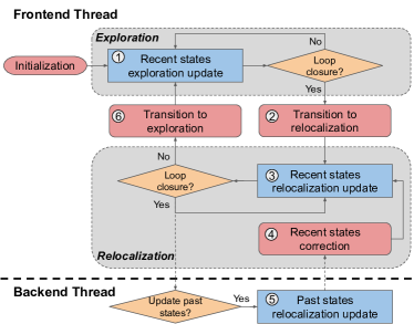
Figure 1: System overview. After initialization, the system starts in exploration mode (Sec. IV-A), and switches to relocalization mode when a set of loop closures is detected (Sec. V-A). When in relocalization mode, besides the frontend thread (Sec. V-B), the system may run a backend thread to perform global adjustment of past states (Sec. V-C), while the frontend thread employs the backend’s feedback (i.e., updated trajectory) to correct recent states (Sec. V-D). Once no loop closures are detected, the system switches back to exploration mode (Sec. IV-B, IV-C).

In what follows, we introduce the key algorithmic components and contributions necessary for realizing the proposed estimation scheme. Specifically, we first provide an overview of the optimal square-root inverse estimator (see Sec. III-A) used during exploration, and then present its Schmidt-based approximation (see Sec. III-B) employed later on for reducing the computational cost of relocalization.

III Square-root Inverse Estimators for SLAM

In this section, we discuss SLAM estimators in the square-root inverse form. We start by denoting the state vector to be estimated as $\mathbf{x}$, which comprises IMU poses and feature positions, and extends with new states as time goes by. At every step, the estimator maintains a prior cost term of the current state estimate, $\left\|\mathbf{R}(\mathbf{x}-\hat{\mathbf{x}})\right\|^{2}$, where $\mathbf{R}$ is the upper-triangular information factor matrix (i.e., the Cholesky factor of the Hessian) and $\hat{\mathbf{x}}$ is the current estimate of $\mathbf{x}$. As new visual or inertial measurements arrive, they contribute another cost term (after linearization), $\left\|\mathbf{H}(\mathbf{x}-\hat{\mathbf{x}})-\mathbf{r}\right\|^{2}$, where $\mathbf{H}$ and $\mathbf{r}$ are the measurement Jacobian and residual, respectively. Then, the updated state estimate, $\hat{\mathbf{x}}^{\oplus}$, is found by minimizing the cost function:

$$\mathcal{C} =\left\|\mathbf{R}(\mathbf{x}-\hat{\mathbf{x}})\right\|^{2}+\left\|\mathbf{H}(\mathbf{x}-\hat{\mathbf{x}})-\mathbf{r}\right\|^{2}$$ (1)

$$\hat{\mathbf{x}}^{\oplus} =\arg\min_{\scriptscriptstyle\mathbf{x}}\mathcal{C}$$ (2)

III-A Optimal Estimator

The optimal solution of (2) can be computed as:

$$\mathcal{C}=\left\|\begin{bmatrix}\mathbf{R}\\ \mathbf{H}\end{bmatrix}\left(\mathbf{x}-\hat{\mathbf{x}}\right)-\begin{bmatrix}\mathbf{0}\\ \mathbf{r}\end{bmatrix}\right\|^{2} =\left\|\begin{bmatrix}\mathbf{R}^{\oplus}\\ \mathbf{0}\end{bmatrix}\left(\mathbf{x}-\hat{\mathbf{x}}\right)-\begin{bmatrix}\mathbf{r}^{\oplus}\\ \mathbf{e}\end{bmatrix}\right\|^{2}$$

$$\Rightarrow\hat{\mathbf{x}}^{\oplus} =\hat{\mathbf{x}}+{\mathbf{R}^{\oplus}}^{-1}\mathbf{r}^{\oplus}$$ (3)

where we have performed the following QR factorization:

$$\begin{bmatrix}\mathbf{R}\\ \mathbf{H}\end{bmatrix}=\mathbf{Q}\begin{bmatrix}\mathbf{R}^{\oplus}\\ \mathbf{0}\end{bmatrix},\ \begin{bmatrix}\mathbf{r}^{\oplus}\\ \mathbf{e}\end{bmatrix}\triangleq\mathbf{Q}^{\scriptscriptstyle{T}}\begin{bmatrix}\mathbf{0}\\ \mathbf{r}\end{bmatrix}$$ (4)

The main advantage of this estimator is its optimality in minimizing the mean square error. Additionally, it is very efficient during the exploration phase, if the states in $\mathbf{x}$ follow a chronological order. Specially, when only local feature-track measurements are available, as described in [11], the QR factorization needs to involve only the bottom-right part of $\mathbf{R}$, which corresponds to recent states. Thus, the cost remains constant, irrespective of the size of the entire state vector $\mathbf{x}$. In contrast, during relocalization, this estimator becomes very inefficient for processing loop-closure measurements, which involve both recent and past states. In this case, the size of the submatrix of $\mathbf{R}$ involved in the QR factorization increases significantly, making the cost at least linear in the size of $\mathbf{x}$. Since this becomes prohibitively expensive, especially when navigating in large areas, in what follows, we introduce alternative approximate estimators that reduce the computational cost, while preserving consistency.

III-B Estimators based on the Schmidt Approximation

As mentioned earlier, the Schmidt approximation, which was introduced originally for the Kalman filter [29], is consistent. The key idea behind it is to save processing cost by updating only a subset of the states while leaving the rest unaltered. In what follows, we discuss its equivalent in the square-root inverse form, identify its limitations, and introduce RISE, an efficient alternative to it. We start by partitioning the state vector $\mathbf{x}$ into two parts: $\mathbf{x}_{\scriptscriptstyle{1}}$ and $\mathbf{x}_{\scriptscriptstyle{2}}$. Now the prior term can be written as

$$\left\|\mathbf{R}(\mathbf{x}-\hat{\mathbf{x}})\right\|^{2}=\left\|\begin{bmatrix}\mathbf{R}_{\scriptscriptstyle 11}&\mathbf{R}_{\scriptscriptstyle 12}\\ &\mathbf{R}_{\scriptscriptstyle 22}\end{bmatrix}\begin{bmatrix}\mathbf{x}_{\scriptscriptstyle{1}}-\hat{\mathbf{x}}_{\scriptscriptstyle{1}}\\ \mathbf{x}_{\scriptscriptstyle{2}}-\hat{\mathbf{x}}_{\scriptscriptstyle{2}}\end{bmatrix}\right\|^{2}$$ (5)

Employing the idea of Schmidt, we use the measurements to update the estimate of $\mathbf{x}_{\scriptscriptstyle{1}}$ to $\hat{\mathbf{x}}_{\scriptscriptstyle{1}}^{\oplus}$ but keep $\hat{\mathbf{x}}_{\scriptscriptstyle{2}}$ the same. By doing so, the posterior term should become

$$\left\|\begin{bmatrix}\mathbf{R}_{\scriptscriptstyle 11}^{\oplus}&\mathbf{R}_{\scriptscriptstyle 12}^{\oplus}\\ &\mathbf{R}_{\scriptscriptstyle 22}\end{bmatrix}\begin{bmatrix}\mathbf{x}_{\scriptscriptstyle{1}}-\hat{\mathbf{x}}_{\scriptscriptstyle{1}}^{\oplus}\\ \mathbf{x}_{\scriptscriptstyle{2}}-\hat{\mathbf{x}}_{\scriptscriptstyle{2}}\end{bmatrix}\right\|^{2}$$ (6)

A property of the Schmidt approximation in this square-root inverse form is that $\mathbf{R}_{\scriptscriptstyle 22}$ remains the same, which does not hold if we change the state order (update $\mathbf{x}_{\scriptscriptstyle{2}}$ but not $\mathbf{x}_{\scriptscriptstyle{1}}$). For this reason, it is preferable to put the states to be updated on the upper part of $\mathbf{x}$. In practice, we typically focus more on recent states than past states, so the states must be organized in reverse chronological order in order to apply the Schmidt approximation. This is in stark contrast to the preferred state order for the case of the optimal estimator during exploration. The ramifications of this order switching will become evident when we discuss them in Sec. IV-V.

Among all Schmidt estimators, the exact Schmidt [29] yields the optimal solution for $\mathbf{x}_{\scriptscriptstyle{1}}$. Surprisingly (and quite unfortunately), its exact equivalent in the inverse form, which we derived in [34], called the inverse Schmidt estimator (ISE), has no speed advantage over the optimal estimator, and causes fill-ins when applied to SLAM. For this reason, in this work we introduce an approximation to ISE, which has lower cost, the resource-aware inverse Schmidt estimator (RISE). This can be derived following the outline in [34] by setting $\mathbf{R}_{\scriptscriptstyle 22}$ to infinity in the steps of ISE, and is summarized hereafter. First, we rewrite the cost function in (2) as

$$\mathcal{C} =\left\|\begin{bmatrix}\mathbf{R}_{\scriptscriptstyle 11}&\mathbf{R}_{\scriptscriptstyle 12}\\ \mathbf{H}_{\scriptscriptstyle{1}}&\mathbf{H}_{\scriptscriptstyle{2}}\end{bmatrix}\begin{bmatrix}\mathbf{x}_{\scriptscriptstyle{1}}-\hat{\mathbf{x}}_{\scriptscriptstyle{1}}\\ \mathbf{x}_{\scriptscriptstyle{2}}-\hat{\mathbf{x}}_{\scriptscriptstyle{2}}\end{bmatrix}-\begin{bmatrix}\mathbf{0}\\ \mathbf{r}\end{bmatrix}\right\|^{2}+\left\|\mathbf{R}_{\scriptscriptstyle 22}(\mathbf{x}_{\scriptscriptstyle{2}}-\hat{\mathbf{x}}_{\scriptscriptstyle{2}})\right\|^{2}$$

$$=\left\|\begin{bmatrix}\mathbf{R}_{\scriptscriptstyle 11}^{\oplus}&\mathbf{R}_{\scriptscriptstyle 12}^{\oplus}\\ &\mathbf{H}_{\scriptscriptstyle{2}}^{\oplus}\\ &\mathbf{R}_{\scriptscriptstyle 22}\end{bmatrix}\begin{bmatrix}\mathbf{x}_{\scriptscriptstyle{1}}-\hat{\mathbf{x}}_{\scriptscriptstyle{1}}\\ \mathbf{x}_{\scriptscriptstyle{2}}-\hat{\mathbf{x}}_{\scriptscriptstyle{2}}\end{bmatrix}-\begin{bmatrix}\mathbf{r}_{\scriptscriptstyle{1}}^{\oplus}\\ \mathbf{e}_{\scriptscriptstyle{1}}\\ \mathbf{0}\end{bmatrix}\right\|^{2}$$ (7)

where the following QR factorization was performed:

$$\begin{bmatrix}\mathbf{R}_{\scriptscriptstyle 11}\\ \mathbf{H}_{\scriptscriptstyle{1}}\end{bmatrix}=\mathbf{Q}_{\scriptscriptstyle{1}}\begin{bmatrix}\mathbf{R}_{\scriptscriptstyle 11}^{\oplus}\\ \mathbf{0}\end{bmatrix}$$ (8)

and

$$\begin{bmatrix}\mathbf{R}_{\scriptscriptstyle 12}^{\oplus}\\ \mathbf{H}_{\scriptscriptstyle{2}}^{\oplus}\end{bmatrix}\triangleq\mathbf{Q}_{\scriptscriptstyle{1}}^{\scriptscriptstyle{T}}\begin{bmatrix}\mathbf{R}_{\scriptscriptstyle 12}\\ \mathbf{H}_{\scriptscriptstyle{2}}\end{bmatrix},\ \begin{bmatrix}\mathbf{r}_{\scriptscriptstyle{1}}^{\oplus}\\ \mathbf{e}_{\scriptscriptstyle{1}}\end{bmatrix}\triangleq\mathbf{Q}_{\scriptscriptstyle{1}}^{\scriptscriptstyle{T}}\begin{bmatrix}\mathbf{0}\\ \mathbf{r}\end{bmatrix}$$ (9)

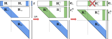
Figure 2: Structure of the information factor when applying RISE. The QR factorization does not involve $\mathbf{R}_{\scriptscriptstyle 22}$. We drop the cost term $\left\|\mathbf{H}_{\scriptscriptstyle{2}}^{\oplus}\left(\mathbf{x}_{\scriptscriptstyle{2}}-\hat{\mathbf{x}}_{\scriptscriptstyle{2}}\right)-\mathbf{e}_{\scriptscriptstyle{1}}\right\|^{2}$, and combine $\mathbf{R}_{\scriptscriptstyle 22}$ with $\mathbf{R}_{\scriptscriptstyle 11}^{\oplus}$ and $\mathbf{R}_{\scriptscriptstyle 12}^{\oplus}$ to form the new cost function $\bar{\mathcal{C}}$ for updating $\mathbf{x}_{\scriptscriptstyle{1}}$, while $\mathbf{x}_{\scriptscriptstyle{2}}$ remains unchanged. Dropping this cost term is the key approximation of RISE. And by ignoring the information in it, we preserve the sparsity of the Cholesky factor.

Next, instead of minimizing $\mathcal{C}$, we drop the cost term $\mathbf{x}_{\scriptscriptstyle{2}}$, $\left\|\mathbf{H}_{\scriptscriptstyle{2}}^{\oplus}\left(\mathbf{x}_{\scriptscriptstyle{2}}-\hat{\mathbf{x}}_{\scriptscriptstyle{2}}\right)-\mathbf{e}_{\scriptscriptstyle{1}}\right\|^{2}$ in (7), and minimize (see Fig. 2):

$$\bar{\mathcal{C}}=\left\|\begin{bmatrix}\mathbf{R}_{\scriptscriptstyle 11}^{\oplus}&\mathbf{R}_{\scriptscriptstyle 12}^{\oplus}\\ &\mathbf{R}_{\scriptscriptstyle 22}\end{bmatrix}\begin{bmatrix}\mathbf{x}_{\scriptscriptstyle{1}}-\hat{\mathbf{x}}_{\scriptscriptstyle{1}}\\ \mathbf{x}_{\scriptscriptstyle{2}}-\hat{\mathbf{x}}_{\scriptscriptstyle{2}}\end{bmatrix}-\begin{bmatrix}\mathbf{r}_{\scriptscriptstyle{1}}^{\oplus}\\ \mathbf{0}\end{bmatrix}\right\|^{2}$$ (10)

Finally, we update the estimate of $\mathbf{x}_{\scriptscriptstyle{1}}$ by setting

$$\hat{\mathbf{x}}_{\scriptscriptstyle{1}}^{\oplus} =\arg\min_{\mathbf{x}_{\scriptscriptstyle{1}}}\bar{\mathcal{C}}=\hat{\mathbf{x}}_{\scriptscriptstyle{1}}+{\mathbf{R}_{\scriptscriptstyle 11}^{\oplus}}^{-1}\mathbf{r}_{\scriptscriptstyle{1}}^{\oplus}$$ (11)

while $\hat{\mathbf{x}}_{\scriptscriptstyle{2}}$ remains unchanged. As a Schmidt estimator, RISE is consistent since it does not assume any state as perfectly known. Instead, it only drops information (the term $\left\|\mathbf{H}_{\scriptscriptstyle{2}}^{\oplus}\left(\mathbf{x}_{\scriptscriptstyle{2}}-\hat{\mathbf{x}}_{\scriptscriptstyle{2}}\right)-\mathbf{e}_{\scriptscriptstyle{1}}\right\|^{2}$), and correctly updates the cross term $\mathbf{R}_{\scriptscriptstyle 12}$ between $\mathbf{x}_{\scriptscriptstyle{1}}$ and $\mathbf{x}_{\scriptscriptstyle{2}}$. As compared to ISE, RISE computes an approximate estimate for $\mathbf{x}_{\scriptscriptstyle{1}}$, whose accuracy loss is negligible when the estimate of $\mathbf{x}_{\scriptscriptstyle{2}}$ is precise. In the extreme case, when the uncertainty of $\mathbf{x}_{\scriptscriptstyle{2}}$ goes to zero, RISE results in the optimal solution for $\mathbf{x}_{\scriptscriptstyle{1}}$ as ISE. For this reason, in practice, we set $\mathbf{x}_{\scriptscriptstyle{2}}$ to be states with low uncertainty. On the other hand, RISE is significantly more efficient than ISE since the cost of the QR factorization is cubic in the size of $\mathbf{x}_{\scriptscriptstyle{1}}$ (instead of $\mathbf{x}$), and introduces no extra fill-ins, thus keeping $\mathbf{R}$ sparse (see the accompanying video for this sparsity in a SLAM simulation). If we select $\mathbf{x}_{\scriptscriptstyle{1}}$ to contain a small number of states (e.g., a window of recent camera poses and features), the cost is O(1) in the size of $\mathbf{x}$. Although the column size of $\mathbf{R}_{\scriptscriptstyle 12}^{\oplus}$ is the same as the size of $\mathbf{x}_{\scriptscriptstyle{2}}$ and can be comparable to that of $\mathbf{x}$, it is sparse in the context of SLAM. As a result, computing $\mathbf{R}_{\scriptscriptstyle 12}^{\oplus}$ is also O(1).

A key advantage of RISE is that it can trade accuracy for speed by adjusting the size of $\mathbf{x}_{\scriptscriptstyle{1}}$. Specifically, during relocalization, we can set $\mathbf{x}_{\scriptscriptstyle{1}}=\mathbf{x}$ to obtain an accurate global adjustment if it is the first loop-closure event, or we can use RISE with a small-size $\mathbf{x}_{\scriptscriptstyle{1}}$ for an approximate but efficient solution. Furthermore, this global adjustment can be split into two steps, where we first employ RISE with a small sized $\mathbf{x}_{\scriptscriptstyle{1}}$, and then we optimize over $\mathbf{x}_{\scriptscriptstyle{2}}$, which can run independently in the backend. Through this process, detailed in Sec. V, the frontend maintains its real-time localization capability, while the backend allows taking advantage of loop-closure events after long periods of exploration.

Note also that the optimal estimator for exploration in Sec. III-A can be considered as a special case of RISE, with $\mathbf{x}_{\scriptscriptstyle{1}}=\mathbf{x}$ and a chronological state order. As it will become evident hereafter, by applying RISE, with different state orders/sizes of $\mathbf{x}_{\scriptscriptstyle{1}}$, in the two phases of SLAM, we can achieve real-time performance while maintaining consistency.

IV RISE-SLAM: Exploration

In this section, we describe how RISE-SLAM processes local feature tracks (see \scriptsize1⃝ in Fig. 1) during exploration. We start with the first exploration (Sec. IV-A), and then discuss the general case, where the system has just switched back to exploration from relocalization (Sec. IV-B and IV-C).

IV-A First Exploration

During the first exploration, we realize the efficiency of the optimal estimator (Sec. III-A) by organizing the states in chronological order [11]. Moreover, we apply RISE with $\mathbf{x}_{\scriptscriptstyle{1}}=\mathbf{x}$, which is equivalent to the optimal estimator. Denote the state vector as $\begin{bmatrix}\mathbf{x}_{\scriptscriptstyle E1}^{\scriptscriptstyle{T}}&\mathbf{x}_{\scriptscriptstyle E2}^{\scriptscriptstyle{T}}\end{bmatrix}^{\scriptscriptstyle{T}}$, where $\mathbf{x}_{\scriptscriptstyle E2}$ comprises a sliding window of recent states involved in the local feature-track measurements, while $\mathbf{x}_{\scriptscriptstyle E1}$ contains all other (previous) states. The cost function to minimize is (see Fig. 3)

$$\mathcal{C}_{\scriptscriptstyle E} =\left\|\begin{bmatrix}\mathbf{R}_{\scriptscriptstyle E11}&\mathbf{R}_{\scriptscriptstyle E12}\\ &\mathbf{R}_{\scriptscriptstyle E22}\end{bmatrix}\begin{bmatrix}\mathbf{x}_{\scriptscriptstyle E1}-\hat{\mathbf{x}}_{\scriptscriptstyle E1}\\ \mathbf{x}_{\scriptscriptstyle E2}-\hat{\mathbf{x}}_{\scriptscriptstyle E2}\end{bmatrix}\right\|^{2}$$

$$\ \ \ +\left\|\mathbf{H}_{\scriptscriptstyle E2}(\mathbf{x}_{\scriptscriptstyle E2}-\hat{\mathbf{x}}_{\scriptscriptstyle E2})-\mathbf{r}_{\scriptscriptstyle E}\right\|^{2}$$ (12)

where the first term is the prior from the previous time step, while the second term corresponds to the new (IMU or feature) measurements. Then, the optimal solution is

$$\hat{\mathbf{x}}_{\scriptscriptstyle E2}^{\oplus} =\hat{\mathbf{x}}_{\scriptscriptstyle E2}+{\mathbf{R}_{\scriptscriptstyle E22}^{\oplus}}^{-1}\mathbf{r}_{\scriptscriptstyle E}^{\oplus}$$ (13)

$$\hat{\mathbf{x}}_{\scriptscriptstyle E1}^{\oplus} =\hat{\mathbf{x}}_{\scriptscriptstyle E1}-\mathbf{R}_{\scriptscriptstyle E11}^{-1}\mathbf{R}_{\scriptscriptstyle E12}{\mathbf{R}_{\scriptscriptstyle E22}^{\oplus}}^{-1}\mathbf{r}_{\scriptscriptstyle E}^{\oplus}$$ (14)

which results from rewriting (12) as

$$\mathcal{C}_{\scriptscriptstyle E} =\left\|\begin{bmatrix}\mathbf{R}_{\scriptscriptstyle E11}&\mathbf{R}_{\scriptscriptstyle E12}\\ &\mathbf{R}_{\scriptscriptstyle E22}^{\oplus}\end{bmatrix}\begin{bmatrix}\mathbf{x}_{\scriptscriptstyle E1}-\hat{\mathbf{x}}_{\scriptscriptstyle E1}^{\oplus}\\ \mathbf{x}_{\scriptscriptstyle E2}-\hat{\mathbf{x}}_{\scriptscriptstyle E2}^{\oplus}\end{bmatrix}\right\|^{2}+\left\|\mathbf{e}_{\scriptscriptstyle E}\right\|^{2}$$ (15)

where $\mathbf{R}_{\scriptscriptstyle E22}^{\oplus}$ is computed by the following QR factorization:

$$\begin{bmatrix}\mathbf{R}_{\scriptscriptstyle E22}\\ \mathbf{H}_{\scriptscriptstyle E2}\end{bmatrix}=\mathbf{Q}_{\scriptscriptstyle E}\begin{bmatrix}\mathbf{R}_{\scriptscriptstyle E22}^{\oplus}\\ \mathbf{0}\end{bmatrix},\ \begin{bmatrix}\mathbf{r}_{\scriptscriptstyle E}^{\oplus}\\ \mathbf{e}_{\scriptscriptstyle E}\end{bmatrix}=\mathbf{Q}_{\scriptscriptstyle E}^{\scriptscriptstyle{T}}\begin{bmatrix}\mathbf{0}\\ \mathbf{r}_{\scriptscriptstyle E}\end{bmatrix}$$ (16)

The impact of this QR factorization on the terms appearing in the cost functions in (12)-(15) is depicted in Fig. 3. These steps are actually analogous to those described in [11], and similarly, the computational complexity is constant and only depends on the size of $\mathbf{x}_{\scriptscriptstyle E2}$. As compared to [11], we improve speed during exploration by limiting both the number of features processed at every step and the feature tracks’ length (since longer tracks offer more accuracy yet diminishing returns, while increasing the processing cost cubically) based on a preselected size of $\mathbf{x}_{\scriptscriptstyle E2}$.

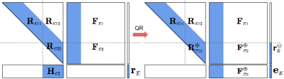
Figure 3: Structure of exploration cost terms before and after an update. $\mathbf{F}_{\scriptscriptstyle E}$ does not exist in Sec. IV-A, while in Sec. IV-C, it contains the cross information between the new and the old map, where the dense columns on the left correspond to some last states of the old map.

IV-B Transition from Relocalization to Exploration

Consider the case when the system is in the relocalization mode (Sec. V) and is about to switch to the exploration mode (i.e., it receives no more loop-closure measurements) (see \scriptsize6⃝ in Fig. 1). Due to the opposite state orderings used in these two modes respectively (Sec. III-B), we first need to change the order of the recent states from reverse chronological, as required in relocalization (Sec. V), to chronological, as for exploration (Sec. IV-A). Specifically, we divide the state vector in relocalization into two parts: $\begin{bmatrix}\mathbf{x}_{\scriptscriptstyle N}^{\prime{\scriptscriptstyle{T}}}&\mathbf{x}_{\scriptscriptstyle M}^{\prime{\scriptscriptstyle{T}}}\end{bmatrix}^{\scriptscriptstyle{T}}$ (the superscript ^′ denotes reverse chronological order), where $\mathbf{x}_{\scriptscriptstyle N}^{\prime}$ contains the recent states where no loop-closure measurements are received. Then, we change the state order of $\mathbf{x}_{\scriptscriptstyle N}^{\prime}$ to chronological, by $\mathbf{x}_{\scriptscriptstyle N}\triangleq\mathbf{P}_{\scriptscriptstyle N}\mathbf{x}_{\scriptscriptstyle N}^{\prime}$ ($\mathbf{P}_{\scriptscriptstyle N}$ is a permutation matrix). Subsequently, we perform a QR factorization to make the permuted Cholesky factor upper-triangular again, which is of constant cost (see [35] for details) regardless of the size of $\mathbf{x}_{\scriptscriptstyle M}^{\prime}$. After these operations, the cost function has the form

$$\mathcal{C}_{\scriptscriptstyle N} =\left\|\begin{bmatrix}\mathbf{R}_{\scriptscriptstyle N11}&\mathbf{R}_{\scriptscriptstyle N12}\\ \end{bmatrix}\begin{bmatrix}\mathbf{x}_{\scriptscriptstyle N}-\hat{\mathbf{x}}_{\scriptscriptstyle N}\\ \mathbf{x}_{\scriptscriptstyle M}^{\prime}-\hat{\mathbf{x}}_{\scriptscriptstyle M}^{\prime}\end{bmatrix}\right\|^{2}+\mathcal{C}_{\scriptscriptstyle M}$$ (17)

where $\mathcal{C}_{\scriptscriptstyle M}=\left\|\mathbf{R}_{\scriptscriptstyle M}\left(\mathbf{x}_{\scriptscriptstyle M}^{\prime}-\hat{\mathbf{x}}_{\scriptscriptstyle M}^{\prime}\right)\right\|^{2}$. Note that the states in $\mathbf{x}_{\scriptscriptstyle M}^{\prime}$ are considered as an old map, which we do not update during the new exploration, so $\mathcal{C}_{\scriptscriptstyle M}$ will not be used in Sec. IV-C.

After this transition step, a new map (comprising new camera poses and features) begins with $\mathbf{x}_{\scriptscriptstyle N}$, while $\mathbf{R}_{\scriptscriptstyle N11}$ represents its information factor and $\mathbf{R}_{\scriptscriptstyle N12}$ the cross information between the two maps.

IV-C Exploration: General Case

In general, when in exploration mode, past map’s states (from previous exploration and relocalization phases) do not need to be updated. Thus, we apply RISE with $\mathbf{x}_{\scriptscriptstyle{2}}=\mathbf{x}_{\scriptscriptstyle M}^{\prime}$ being the past map’s states, while $\mathbf{x}_{\scriptscriptstyle{1}}=\mathbf{x}_{\scriptscriptstyle N}$ comprises the new map’s states which expand as the current exploration goes on. Specifically, the same operations as for the first exploration (Sec. IV-A) are applied to the new map’s states. Additionally, as explained in Sec. III-B, the RISE applies the QR transformation in (16) on the cross information term $\mathbf{F}_{\scriptscriptstyle E}$ (originally starts as $\mathbf{R}_{\scriptscriptstyle N12}$ in (17) and evolves with time), as shown in Fig. 3, and drops the cost term $\left\|\mathbf{F}_{\scriptscriptstyle E3}^{\oplus}\left(\mathbf{x}_{\scriptscriptstyle M}^{\prime}-\hat{\mathbf{x}}_{\scriptscriptstyle M}^{\prime}\right)-\mathbf{e}_{\scriptscriptstyle E}\right\|^{2}$ involving only the old map’s states (see [35] for a detailed derivation). Note that only the lower of part of $\mathbf{F}_{\scriptscriptstyle E}$, $\mathbf{F}_{\scriptscriptstyle E2}$, which has a bounded number of dense columns, needs updating. Thus, the computational complexity for the general case of exploration with RISE is also constant.

V RISE-SLAM: Relocalization

We now consider the case, where the system switches from exploration to relocalization mode so as to use loop-closure measurements for global pose and map correction.

V-A Transition from Exploration to Relocalization

Before entering relocalization, we need to switch the state order from chronological to reverse chronological. Specifically, during exploration, the state vector is in the form $\begin{bmatrix}\mathbf{x}_{\scriptscriptstyle L}^{{\scriptscriptstyle{T}}}&\mathbf{x}_{\scriptscriptstyle M}^{\prime{\scriptscriptstyle{T}}}\end{bmatrix}^{\scriptscriptstyle{T}}$, where $\mathbf{x}_{\scriptscriptstyle L}$ comprises all states in the current map, while $\mathbf{x}_{\scriptscriptstyle M}^{\prime}$ corresponds to the old map [see (17) and Sec. IV-C]. We first change the state order of $\mathbf{x}_{\scriptscriptstyle L}$ to reverse chronological by defining $\mathbf{x}_{\scriptscriptstyle L}^{\prime}\triangleq\mathbf{P}_{\scriptscriptstyle L}\mathbf{x}_{\scriptscriptstyle L}$ ($\mathbf{P}_{\scriptscriptstyle L}$ is a permutation matrix). Then, we split $\mathbf{x}_{\scriptscriptstyle L}^{\prime}$ into two parts: $\mathbf{x}_{\scriptscriptstyle L1}^{\prime}$ comprises the recent states to be maintained in the frontend, while the remaining states $\mathbf{x}_{\scriptscriptstyle L2}^{\prime}$ are combined with the old map $\mathbf{x}_{\scriptscriptstyle M}^{\prime}$ so as to be optimized by the backend ($\mathbf{x}_{\scriptscriptstyle B}^{\prime}\triangleq\begin{bmatrix}\mathbf{x}_{\scriptscriptstyle L2}^{\prime{\scriptscriptstyle{T}}}&\mathbf{x}_{\scriptscriptstyle M}^{\prime{\scriptscriptstyle{T}}}\end{bmatrix}^{\scriptscriptstyle{T}}$). Accordingly, in terms of cost functions, we first combine all available cost terms so far, including the current exploration (Fig. 3) and the old map $\mathcal{C}_{\scriptscriptstyle M}$ from (17) [first term in (18)], and the new loop-closure measurements [second term in (18)], to get the total cost $\mathcal{C}_{\scriptscriptstyle T}$. Then, we employ the QR factorization of RISE [see (7)-(9)] to split $\mathcal{C}_{\scriptscriptstyle T}$ into two parts:

$$\mathcal{C}_{\scriptscriptstyle T} =\left\|\begin{bmatrix}\mathbf{R}_{\scriptscriptstyle T11}&\mathbf{R}_{\scriptscriptstyle T12}\\ &\mathbf{R}_{\scriptscriptstyle T22}\end{bmatrix}\begin{bmatrix}\mathbf{x}_{\scriptscriptstyle L1}^{\prime}-\hat{\mathbf{x}}_{\scriptscriptstyle L1}^{\prime}\\ \mathbf{x}_{\scriptscriptstyle B}^{\prime}-\hat{\mathbf{x}}_{\scriptscriptstyle B}^{\prime}\end{bmatrix}\right\|^{2}$$

$$\ \ \ +\left\|\mathbf{H}_{\scriptscriptstyle T1}(\mathbf{x}_{\scriptscriptstyle L1}^{\prime}-\hat{\mathbf{x}}_{\scriptscriptstyle L1}^{\prime})+\mathbf{H}_{\scriptscriptstyle T2}(\mathbf{x}_{\scriptscriptstyle B}^{\prime}-\hat{\mathbf{x}}_{\scriptscriptstyle B}^{\prime})-\mathbf{r}_{\scriptscriptstyle T}\right\|^{2}$$ (18)

$$=\left\|\begin{bmatrix}\mathbf{R}_{\scriptscriptstyle T11}^{\oplus}&\mathbf{R}_{\scriptscriptstyle T12}^{\oplus}\\ &\mathbf{R}_{\scriptscriptstyle T22}\\ &\mathbf{H}_{\scriptscriptstyle T2}^{\oplus}\end{bmatrix}\begin{bmatrix}\mathbf{x}_{\scriptscriptstyle L1}^{\prime}-\hat{\mathbf{x}}_{\scriptscriptstyle L1}^{\prime}\\ \mathbf{x}_{\scriptscriptstyle B}^{\prime}-\hat{\mathbf{x}}_{\scriptscriptstyle B}^{\prime}\end{bmatrix}-\begin{bmatrix}\mathbf{r}_{\scriptscriptstyle T}^{\oplus}\\ \mathbf{0}\\ \mathbf{e}_{\scriptscriptstyle T}\end{bmatrix}\right\|^{2}=\mathcal{C}_{\scriptscriptstyle F}+\mathcal{C}_{\scriptscriptstyle B}$$ (19)

where

$$\mathcal{C}_{\scriptscriptstyle F} \triangleq\left\|\mathbf{R}_{\scriptscriptstyle T11}^{\oplus}(\mathbf{x}_{\scriptscriptstyle L1}^{\prime}-\hat{\mathbf{x}}_{\scriptscriptstyle L1}^{\prime\oplus})+\mathbf{R}_{\scriptscriptstyle T12}^{\oplus}(\mathbf{x}_{\scriptscriptstyle B}^{\prime}-\hat{\mathbf{x}}_{\scriptscriptstyle B}^{\prime})\right\|^{2}$$ (20)

$$\hat{\mathbf{x}}_{\scriptscriptstyle L1}^{\prime\oplus} \triangleq\hat{\mathbf{x}}_{\scriptscriptstyle L1}^{\prime}+\mathbf{R}_{\scriptscriptstyle T11}^{\oplus-1}\mathbf{r}_{\scriptscriptstyle T}^{\oplus}$$ (21)

$$\mathcal{C}_{\scriptscriptstyle B} \triangleq\left\|\begin{bmatrix}\mathbf{R}_{\scriptscriptstyle T22}\\ \mathbf{H}_{\scriptscriptstyle T2}^{\oplus}\end{bmatrix}(\mathbf{x}_{\scriptscriptstyle B}^{\prime}-\hat{\mathbf{x}}_{\scriptscriptstyle B}^{\prime})-\begin{bmatrix}\mathbf{0}\\ \mathbf{e}_{\scriptscriptstyle T}\end{bmatrix}\right\|^{2}$$ (22)

Among the operations required in this transition step, the frontend only needs a small-size matrix QR factorization to obtain $\mathcal{C}_{\scriptscriptstyle F}$ with constant cost, while all the (expensive) remaining work is done in the backend (see [35] for details).

After this transition step, in the frontend $\mathcal{C}_{\scriptscriptstyle F}$ is extended to include information from new poses and features and minimized to update a sliding window of recent states (starting from $\mathbf{x}_{\scriptscriptstyle L1}^{\prime}$). Meanwhile, in the backend, $\mathcal{C}_{\scriptscriptstyle B}$ is minimized to provide global corrections for the past states $\mathbf{x}_{\scriptscriptstyle B}^{\prime}$.

V-B Relocalization: Frontend Thread

The relocalization frontend employs RISE to process both local feature tracks and loop-closure measurements so as to update a sliding window of recent states (see \scriptsize3⃝ in Fig. 1). Specifically, the cost function $\mathcal{C}_{\scriptscriptstyle R}$, to be optimized in the frontend, extends from $\mathcal{C}_{\scriptscriptstyle F}$ in (20) and has the form

$$\mathcal{C}_{\scriptscriptstyle R} =\left\|\begin{bmatrix}\mathbf{R}_{\scriptscriptstyle R11}&\mathbf{R}_{\scriptscriptstyle R12}\\ &\mathbf{R}_{\scriptscriptstyle R22}\end{bmatrix}\begin{bmatrix}\mathbf{x}_{\scriptscriptstyle R1}^{\prime}-\hat{\mathbf{x}}_{\scriptscriptstyle R1}^{\prime}\\ \mathbf{x}_{\scriptscriptstyle R2}^{\prime}-\hat{\mathbf{x}}_{\scriptscriptstyle R2}^{\prime}\end{bmatrix}\right\|^{2}$$

$$\ \ \ +\left\|\begin{bmatrix}\mathbf{H}_{\scriptscriptstyle R1}&\mathbf{H}_{\scriptscriptstyle R2}\end{bmatrix}\begin{bmatrix}\mathbf{x}_{\scriptscriptstyle R1}^{\prime}-\hat{\mathbf{x}}_{\scriptscriptstyle R1}^{\prime}\\ \mathbf{x}_{\scriptscriptstyle R2}^{\prime}-\hat{\mathbf{x}}_{\scriptscriptstyle R2}^{\prime}\end{bmatrix}-\mathbf{r}_{\scriptscriptstyle R}\right\|^{2}$$ (23)

where $\mathbf{x}_{\scriptscriptstyle R1}^{\prime}$ contains the window of recent states to be updated at the current step, while $\mathbf{x}_{\scriptscriptstyle R2}^{\prime}$ represents all previous states (including $\mathbf{x}_{\scriptscriptstyle B}^{\prime}$) whose estimates are kept unchanged in the frontend. The measurement Jacobians $\mathbf{H}_{\scriptscriptstyle R1}$ and $\mathbf{H}_{\scriptscriptstyle R2}$ are both nonzero (see Fig. 4) since here we consider both local feature tracks and loop-closure measurements. Then, the frontend employs RISE to update only $\mathbf{x}_{\scriptscriptstyle R1}^{\prime}$ by first performing the QR factorization to transform $\mathcal{C}_{\scriptscriptstyle R}$ from (23) into

$$\mathcal{C}_{\scriptscriptstyle R} =\left\|\begin{bmatrix}\mathbf{R}_{\scriptscriptstyle R11}^{\oplus}&\mathbf{R}_{\scriptscriptstyle R12}^{\oplus}\\ &\mathbf{H}_{\scriptscriptstyle R2}^{\oplus}\end{bmatrix}\begin{bmatrix}\mathbf{x}_{\scriptscriptstyle R1}^{\prime}-\hat{\mathbf{x}}_{\scriptscriptstyle R1}^{\prime}\\ \mathbf{x}_{\scriptscriptstyle R2}^{\prime}-\hat{\mathbf{x}}_{\scriptscriptstyle R2}^{\prime}\end{bmatrix}-\begin{bmatrix}\mathbf{r}_{\scriptscriptstyle R}^{\oplus}\\ \mathbf{e}_{\scriptscriptstyle R}\end{bmatrix}\right\|^{2}$$

$$\ \ \ +\left\|\mathbf{R}_{\scriptscriptstyle R22}(\mathbf{x}_{\scriptscriptstyle R2}^{\prime}-\hat{\mathbf{x}}_{\scriptscriptstyle R2}^{\prime})\right\|^{2}$$ (24)

and then dropping the term $\left\|\mathbf{H}_{\scriptscriptstyle R2}^{\oplus}(\mathbf{x}_{\scriptscriptstyle R2}^{\prime}-\hat{\mathbf{x}}_{\scriptscriptstyle R2}^{\prime})-\mathbf{e}_{\scriptscriptstyle R}\right\|^{2}$ (since we are not updating $\mathbf{x}_{\scriptscriptstyle R2}^{\prime}$) to get $\bar{\mathcal{C}}_{\scriptscriptstyle R}$

$$\bar{\mathcal{C}}_{\scriptscriptstyle R} =\left\|\begin{bmatrix}\mathbf{R}_{\scriptscriptstyle R11}^{\oplus}&\mathbf{R}_{\scriptscriptstyle R12}^{\oplus}\\ &\mathbf{R}_{\scriptscriptstyle R22}\end{bmatrix}\begin{bmatrix}\mathbf{x}_{\scriptscriptstyle R1}^{\prime}-\hat{\mathbf{x}}_{\scriptscriptstyle R1}^{\prime\oplus}\\ \mathbf{x}_{\scriptscriptstyle R2}^{\prime}-\hat{\mathbf{x}}_{\scriptscriptstyle R2}^{\prime}\end{bmatrix}\right\|^{2}$$ (25)

$$\hat{\mathbf{x}}_{\scriptscriptstyle R1}^{\prime\oplus} \triangleq\hat{\mathbf{x}}_{\scriptscriptstyle R1}^{\prime}+\mathbf{R}_{\scriptscriptstyle R11}^{\oplus-1}\mathbf{r}_{\scriptscriptstyle R}^{\oplus}$$ (26)

where $\hat{\mathbf{x}}_{\scriptscriptstyle R1}^{\prime\oplus}$ is the updated state estimate. The structural changes of the factors appearing in (23)-(24) are shown in Fig. 4. The processing cost of this update is defined by the QR factorization, and is constant since the size of $\mathbf{x}_{\scriptscriptstyle R1}^{\prime}$ and the number of dense columns in $\mathbf{R}_{\scriptscriptstyle R12}^{\oplus}$ are bounded. Due to its low processing cost, the frontend thread is able to update the states at high frequency in real time.

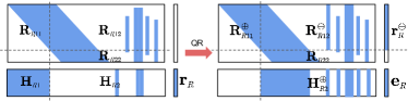
Figure 4: Structure of the factors corresponding to the relocalization cost terms before and after a RISE update in the frontend.

V-C Relocalization: Backend Thread

The backend performs global adjustment so as to accurately update a large number of past states, while running in parallel with the frontend to avoid blocking it (see \scriptsize5⃝ in Fig. 1). Within RISE, the backend can run whenever the thread is idle, to increase accuracy. In our current design, however, in order to save processing, we choose to run it only once during each relocalization phase, right after the transition step described in Sec. V-A, and update all the past states to obtain the optimal solution. Specifically, from (22), we compute the optimal estimate of the past states $\mathbf{x}_{\scriptscriptstyle B}^{\prime}$ by minimizing the cost function $\mathcal{C}_{\scriptscriptstyle B}$, which is a batch least-squares problem and can be solved by employing a sparse QR factorization. Once the new estimate $\hat{\mathbf{x}}_{\scriptscriptstyle B}^{\prime\oplus}$ is obtained, $\mathcal{C}_{\scriptscriptstyle B}$ can be rewritten as (after ignoring a constant term)

$$\mathcal{C}_{\scriptscriptstyle B}=\left\|\mathbf{R}_{\scriptscriptstyle B}(\mathbf{x}_{\scriptscriptstyle B}^{\prime}-\hat{\mathbf{x}}_{\scriptscriptstyle B}^{\prime\oplus})\right\|^{2}$$ (27)

The computational cost is approximately linear in the (large) size of $\mathbf{x}_{\scriptscriptstyle B}^{\prime}$, but it does not prevent the frontend from performing real-time estimation since they run in parallel.

V-D Feedback from Backend to Frontend Thread

After the backend finishes a global update on the past states $\mathbf{x}_{\scriptscriptstyle B}^{\prime}$, the frontend employs this result to update the recent states so that they benefit from the global correction (see \scriptsize4⃝ in Fig. 1). Specifically, if we denote all the recent states accumulated in the frontend since the backend started as $\mathbf{x}_{\scriptscriptstyle F}^{\prime}$, then from (25) and Fig. 4, the frontend maintains a cost term of the form $\left\|\mathbf{R}_{\scriptscriptstyle F}(\mathbf{x}_{\scriptscriptstyle F}^{\prime}-\hat{\mathbf{x}}_{\scriptscriptstyle F}^{\prime})+\mathbf{R}_{\scriptscriptstyle FB}(\mathbf{x}_{\scriptscriptstyle B}^{\prime}-\hat{\mathbf{x}}_{\scriptscriptstyle B}^{\prime})\right\|^{2}$, where the information factor $\mathbf{R}_{F}$ is upper-triangular and $\mathbf{R}_{FB}$ represents the cross information between the states in the frontend and the backend. Combining this frontend’s cost term with that of the backend [$\mathcal{C}_{\scriptscriptstyle B}$ in (27)] yields

$$\mathcal{C}_{\scriptscriptstyle FB} =\left\|\mathbf{R}_{\scriptscriptstyle F}(\mathbf{x}_{\scriptscriptstyle F}^{\prime}-\hat{\mathbf{x}}_{\scriptscriptstyle F}^{\prime})+\mathbf{R}_{\scriptscriptstyle FB}(\mathbf{x}_{\scriptscriptstyle B}^{\prime}-\hat{\mathbf{x}}_{\scriptscriptstyle B}^{\prime})\right\|^{2}$$

$$\ \ \ +\left\|\mathbf{R}_{\scriptscriptstyle B}(\mathbf{x}_{\scriptscriptstyle B}^{\prime}-\hat{\mathbf{x}}_{\scriptscriptstyle B}^{\prime\oplus})\right\|^{2}$$

$$=\left\|\begin{bmatrix}\mathbf{R}_{\scriptscriptstyle F}&\mathbf{R}_{\scriptscriptstyle FB}\\ &\mathbf{R}_{\scriptscriptstyle B}\end{bmatrix}\begin{bmatrix}\mathbf{x}_{\scriptscriptstyle F}^{\prime}-\hat{\mathbf{x}}_{\scriptscriptstyle F}^{\prime\oplus}\\ \mathbf{x}_{\scriptscriptstyle B}^{\prime}-\hat{\mathbf{x}}_{\scriptscriptstyle B}^{\prime\oplus}\end{bmatrix}\right\|^{2}$$ (28)

$$\hat{\mathbf{x}}_{\scriptscriptstyle F}^{\prime\oplus} \triangleq\hat{\mathbf{x}}_{\scriptscriptstyle F}^{\prime}+\mathbf{R}_{\scriptscriptstyle F}^{-1}\mathbf{R}_{\scriptscriptstyle FB}\left(\hat{\mathbf{x}}_{\scriptscriptstyle B}^{\prime}-\hat{\mathbf{x}}_{\scriptscriptstyle B}^{\prime\oplus}\right)$$ (29)

where $\hat{\mathbf{x}}_{\scriptscriptstyle F}^{\prime\oplus}$ is the globally corrected estimate for the recent states in the frontend. The operations required in (29) are sparse matrix-vector multiplications and back substitutions, which are faster than the operations of Sec. V-B in practice.

As a result of this step, all current states in the frontend are immediately corrected using the globally adjusted estimates from the backend. Note that, this is a key difference between our algorithm and existing multi-thread SLAM systems. Specifically, [3, 6, 8] solve separate optimization problems independently in different threads; hence their frontend has to rely on map reobservations after the backend’s global adjustment finishes in order to obtain corrections. This is due to the fact that the two sets of states involved in their frontend’s and backend’s (separate) optimization problems are considered uncorrelated. In contrast, our algorithm always solves a single optimization problem over two correlated sets of states [see (28)], carried out in two separate threads. Consequently, as soon as the corrections from the backend become available, they immediately affect the frontend’s states, even if the map is not reobserved.

VI Experimental Results

To evaluate the performance of the proposed RISE-SLAM, we compared it against state-of-the-art visual-inertial SLAM estimators, including a visual-inertial odometry (VIO) system without loop closures (OKVIS [5]), and SLAM systems with loop closures (VINS-Mono [6], ICE-BA [8]), using the EuRoC [36] datasets. Since our implementation focuses on visual-inertial SLAM, we did not compare to vision-only systems, such as [3]. The datasets contain stereo images (only the left-camera images are used) from global shutter cameras (20 Hz) and IMU measurements (200 Hz), along with ground-truth poses from VICON. The code of each compared system is downloaded from their Github repositories and run with the provided configuration files for the EuRoC datasets.

VI-A System Setup

In our implementation, we extract 300 ORB [37] features per image and match them based on their descriptors against previous images to generate feature tracks. Loop-closure measurements are provided by a vocabulary tree [38], and the system switches to relocalization mode when detecting features that have not been observed for more than 15 sec. We model the noise of all visual observations as zero-mean white Gaussian with $\sigma=1.5$ pixels. During both exploration and relocalization, the frontend updates a sliding window corresponding to 10 recent poses and their observed features. To improve efficiency, feature tracks longer than 20 are split into multiple shorter ones while the number of feature tracks being processed per time step is limited to 40.

VI-B Localization Accuracy

We compute the root-mean-square error (RMSE) of the estimated positions as compared to the ground truth, to evaluate the tracking accuracy of all estimators considered. Each estimated trajectory is aligned with the ground-truth coordinate frame by a 3D-to-3D matching using [39].

For fairness, we first run the proposed RISE-SLAM without using any loop-closure measurements [RISE (vio)] so as to compare it with the VIO system OKVIS. Then, we add loop-closure measurements [RISE (lc)] to compare it with the SLAM systems VINS-Mono and ICE-BA. The position RMSE results from all EuRoC datasets are shown in Table I. As shown, our RISE (vio) outperforms OKVIS on all datasets. This is due to the fact that RISE optimally processes all available measurements during exploration (see Sec. IV-A). Among the SLAM systems, ICE-BA performs the worst. This is probably because loop closure is not implemented yet in their public code, which makes their system a VIO with a backend that performs global smoothing. Regardless, ICE-BA does not achieve better accuracy even when compared to RISE (vio), while requiring more CPU resources for running a backend thread. Meanwhile, our RISE (lc) is the best on most of the datasets, and outperforms VINS-Mono. An example of the RISE-SLAM estimated trajectory vs. ground truth is shown in the accompanying video.

TABLE I: Position RMSE (cm) on EuRoC datasets

Dataset	RISE (vio)	OKVIS	RISE (lc)	VINS-Mono	ICE-BA
MH_01_easy	16.1	34.6	5.1	8.8	16.4
MH_02_easy	19.3	40.9	12.0	6.3	8.9
MH_03_medium	21.9	22.1	8.4	8.5	17.2
MH_04_difficult	24.1	33.7	16.1	17.5	31.6
MH_05_difficult	30.5	42.5	25.6	14.5	31.4
V1_01_easy	5.1	10.6	4.1	4.5	5.2
V1_02_medium	7.0	11.6	3.3	6.5	11.7
V1_03_difficult	11.6	22.7	6.7	29.9	11.1
V2_01_easy	6.6	16.2	5.5	6.4	9.1
V2_02_medium	10.4	18.1	4.0	13.3	11.5
V2_03_difficult	10.1	28.5	11.7	18.0	12.8
Average	14.8	25.6	9.3	12.2	15.2

VI-C Computational Efficiency

We run all algorithms on a laptop with Intel Core i7-6700HQ 2.60GHz x 8 CPU to compare the efficiency of each estimator. Since we focus on estimation speed, we do not consider the cost of image processing. Average times of one run are shown in Table II. Note that since RISE-SLAM has two modes with different costs, we report the averages of exploration and relocalization (the time of transition steps is also included), respectively, as well as the overall average across all runs. As expected, the exploration is typically faster than relocalization since it only processes local feature tracks. As evident from Table II, RISE-SLAM is significantly faster than VINS-Mono and OKVIS. Only ICE-BA runs as fast as RISE-SLAM, but has lower tracking accuracy.

TABLE II: Average running time (msec) of one estimator run

RISE	RISE	RISE	OKVIS	VINS-Mono	ICE-BA
exploration	relocalization	overall
10	13	11	26	52	11

VI-D Estimation Consistency

To assess the consistency improvement of RISE as compared to estimators that assume some past states to be perfectly known, we employ the normalized estimation error squared (NEES) [40]. Typically more overconfident (inconsistent) estimates yield larger NEES. To isolate the effect of other factors affecting consistency (e.g., linearization, local minima, outliers), we first evaluate NEES in Monte Carlo simulations where the camera follows a circular path twice. In this case, the RISE-SLAM’s position NEES fluctuates between 5 and 100, while if the map is assumed perfectly-known the NEES ranges from 10 to 2,500. Furthermore, on the EuRoC datasets, VINS-Mono, which assumes perfectly-known keyframe poses, has a median position NEES of over 100, while that of RISE-SLAM is $\sim$40 (see [35] for details).

VII Conclusion

Motivated by the consistency guarantees and the linear processing cost of the Schmidt Kalman filter, as well as the linear memory requirements of the Cholesky factor of maps computed online, in this work, we introduce the resource-aware inverse Schmidt estimator (RISE), an approximation to the exact inverse Schmidt, that maintains the sparsity of the Cholesky factor and allows us to improve consistency. Furthermore, we employ different (in terms of the order and number of states involved) configurations of RISE to form the frontend and backend of a visual-inertial system, RISE-SLAM, which appropriately treats the exploration versus the relocalization phases of SLAM to achieve real-time operation. As demonstrated by the experimental evaluation, RISE-SLAM achieves position accuracy typically better than alternative state-of-the-art visual-inertial estimators, at lower processing cost while improving estimation consistency.

References

- [1] G. Klein and D. Murray, “Parallel tracking and mapping for small AR workspaces,” in Proc. of the IEEE International Symposium on Mixed and Augmented Reality, Nara, Japan, Nov.11–16 2007, pp. 225–234.
- [2] J. Engel, T. Schöps, and D. Cremers, “LSD-SLAM: Large-scale direct monocular SLAM,” in Proc. of the European Conference on Computer Vision, Zurich, Switzerland, Sept.6–12 2014, pp. 834–849.
- [3] R. Mur-Artal, J. M. M. Montiel, and J. D. Tardos, “ORB-SLAM: A versatile and accurate monocular slam system,” IEEE Trans. on Robotics, vol. 31, no. 5, pp. 1147–1163, 2015.
- [4] A. I. Mourikis and S. I. Roumeliotis, “A multi-state constraint Kalman filter for vision-aided inertial navigation,” in Proc. of the IEEE International Conference on Robotics and Automation, Rome, Italy, Apr. 10–14 2007, pp. 3482–3489.
- [5] S. Leutenegger, S. Lynen, M. Bosse, R. Siegwart, and P. Furgale, “Keyframe-based visual-inertial odometry using nonlinear optimization,” International Journal of Robotics Research, vol. 34, no. 3, pp. 314–334, March 2015.
- [6] T. Qin, P. Li, and S. Shen, “Vins-mono: A robust and versatile monocular visual-inertial state estimator,” IEEE Trans. on Robotics, vol. 34, no. 99, pp. 1–17, 2018.
- [7] R. Mur-Artal and J. D. Tardós, “Visual-inertial monocular SLAM with map reuse,” IEEE Robotics and Automation Letters, vol. 2, no. 2, pp. 796–803, 2017.
- [8] H. Liu, M. Chen, G. Zhang, H. Bao, and Y. Bao, “ICE-BA: Incremental, consistent and efficient bundle adjustment for visual-inertial SLAM,” in Proc. of the IEEE Conference on Computer Vision and Pattern Recognition, Salt Lake City, UT, June18-22 2018, pp. 1974–1982.
- [9] B. Triggs, P. F. McLauchlan, R. I. Hartley, and A. W. Fitzgibbon, “Bundle adjustment - a modern synthesis,” in Proc. of the International Workshop on Vision Algorithms: Theory and Practice, ser. Lecture Notes in Computer Science, vol. 1883, Corfu, Greece, September 21-22 1999, pp. 298–372.
- [10] F. Dellaert and M. Kaess, “Square root sam: Simultaneous localization and mapping via square root information smoothing,” International Journal of Robotics Research, vol. 25, no. 12, pp. 1181–1203, December 2006.
- [11] M. Kaess, A. Ranganathan, and F. Dellaert, “iSAM: Incremental smoothing and mapping,” IEEE Trans. on Robotics, vol. 24, no. 6, pp. 1365–1378, December 2008.
- [12] M. Kaess, H. Johannsson, R. Roberts, V. Ila, J. Leonard, and F. Dellaert, “iSAM2: Incremental smoothing and mapping using the bayes tree,” International Journal of Robotics Research, vol. 31, no. 2, pp. 216–235, February 2012.
- [13] J. Engel, J. Sturm, and D. Cremers, “Semi-dense visual odometry for a monocular camera,” in Proc. of the IEEE International Conference on Computer Vision, Sydney, Australia, Dec.1–8 2013, pp. 1449–1456.
- [14] J. A. Hesch, D. G. Kottas, S. L. Bowman, and S. I. Roumeliotis, “Consistency analysis and improvement of vision-aided inertial navigation,” IEEE Trans. on Robotics, vol. 30, no. 1, pp. 158–176, 2014.
- [15] K. J. Wu, A. Ahmed, G. Georgiou, and S. I. Roumeliotis, “A square root inverse filter for efficient vision-aided inertial navigation on mobile devices,” in Proc. of Robotics: Science and Systems, Rome, Italy, July 13 – 17 2015.
- [16] C. Forster, Z. Zhang, M. Gassner, M. Werlberger, and D. Scaramuzza, “SVO: Semidirect visual odometry for monocular and multicamera systems,” IEEE Trans. on Robotics, vol. 33, no. 2, pp. 249–265, 2017.
- [17] M. Bloesch, M. Burri, S. Omari, M. Hutter, and R. Siegwart, “Iterated extended Kalman filter based visual-inertial odometry using direct photometric feedback,” The International Journal of Robotics Research, vol. 36, no. 10, pp. 1053–1072, 2017.
- [18] J. Engel, V. Koltun, and D. Cremers, “Direct sparse odometry,” IEEE Trans. on Pattern Analysis and Machine Intelligence, vol. 40, no. 3, pp. 611–625, March 2018.
- [19] S. Thrun and M. Montemerlo, “The graph SLAM algorithm with applications to large-scale mapping of urban structures,” The International Journal of Robotics Research, vol. 25, no. 5-6, pp. 403–429, 2006.
- [20] K. Konolige and M. Agrawal, “Frameslam: From bundle adjustment to real-time visual mapping,” IEEE Trans. on Robotics, vol. 24, no. 5, pp. 1066–1077, Oct 2008.
- [21] E. D. Nerurkar, K. J. Wu, and S. I. Roumeliotis, “C-KLAM: Constrained keyframe-based localization and mapping for long-term navigation,” in Proc. of the IEEE International Conference on Robotics and Automation, Hong Kong, China, May 31 – June 7 2014, pp. 3638–3643.
- [22] S. J. Julier and J. K. Uhlmann, “A non-divergent estimation algorithm in the presence of unknown correlations,” in Proc. of the American Control Conference, vol. 4, Albuquerque, NM, June 4–6 1997, pp. 2369–2373.
- [23] A. H. Jazwinski, Stochastic Processes and Filtering Theory. New York, NY: Academic Press, 1970.
- [24] G. P. Huang, A. I. Mourikis, and S. I. Roumeliotis, “Observability-based rules for designing consistent ekf slam estimators,” International Journal of Robotics Research, vol. 29, no. 5, pp. 502–528, Apr. 2010.
- [25] A. I. Mourikis, N. Trawny, S. I. Roumeliotis, A. E. Johson, A. Ansar, and L. Matthies, “Vision-aided inertial navigation for spacecraft entry, descent, and landing,” IEEE Trans. on Robotics, vol. 25, no. 2, pp. 264–280, Apr. 2009.
- [26] S. Lynen, T. Sattler, M. Bosse, J. Hesch, M. Pollefeys, and R. Siegwart, “Get out of my lab: Large-scale, real-time visual-inertial localization,” in Proc. of Robotics: Science and Systems, Rome, Italy, July 13-17 2015.
- [27] S. Thrun, Y. Liu, D. Koller, A. Y. Ng, Z. Ghahramani, and H. Durrant-Whyte, “Simultaneous localization and mapping with sparse extended information filters,” International Journal of Robotics Research, vol. 23, no. 7-8, pp. 693–716, August 2004.
- [28] M. R. Walter, R. M. Eustice, and J. J. Leonard, “Exactly sparse extended information filters for feature-based SLAM,” International Journal of Robotics Research, vol. 26, no. 4, pp. 335–359, April 2007.
- [29] S. F. Schmidt, “Application of state-space methods to navigation problems,” in Advances in control systems. Elsevier, 1966, vol. 3, pp. 293–340.
- [30] J. E. Guivant and E. M. Nebot, “Optimization of the simultaneous localization and map-building algorithm for real-time implementation,” IEEE Trans. on Robotics and Automation, vol. 17, no. 3, pp. 242–257, 2001.
- [31] S. J. Julier, “A sparse weight Kalman filter approach to simultaneous localisation and map building,” in Proc. of the IEEE/RSJ International Conference on Intelligent Robots and Systems, vol. 3, Maui, HI, Oct. 29 – Nov. 3 2001, pp. 1251–1256.
- [32] E. D. Nerurkar and S. I. Roumeliotis, “Power-SLAM: A linear-complexity, anytime algorithm for SLAM,” The International Journal of Robotics Research, vol. 30, no. 6, pp. 772–788, 2011.
- [33] R. C. DuToit, J. A. Hesch, E. D. Nerurkar, and S. I. Roumeliotis, “Consistent map-based 3D localization on mobile devices,” in Proc. of the IEEE International Conference on Robotics and Automation, 2017, pp. 6253–6260.
- [34] K. J. Wu and S. I. Roumeliotis, “Inverse Schmidt estimators,” http://mars.cs.umn.edu/tr/inverseschmidt.pdf.
- [35] T. Ke, K. J. Wu, and S. I. Roumeliotis, “Visual-inertial SLAM with inverse Schmidt estimators,” http://mars.cs.umn.edu/tr/risetechreport.pdf.
- [36] M. Burri, J. Nikolic, P. Gohl, T. Schneider, J. Rehder, S. Omari, M. W. Achtelik, and R. Siegwart, “The EuRoC micro aerial vehicle datasets,” The International Journal of Robotics Research, vol. 35, no. 10, pp. 1157–1163, Sept. 2016.
- [37] E. Rublee, V. Rabaud, K. Konolige, and G. Bradski, “ORB: An efficient alternative to SIFT or SURF,” in Proc. of the IEEE International Conference on Computer Vision, Barcelona, Spain, Nov. 6–13 2011, pp. 2564–2571.
- [38] D. Nister and H. Stewenius, “Scalable recognition with a vocabulary tree,” in Proc. of the IEEE Conference on Computer Vision and Pattern Recognition, vol. 2, New York, NY, June17–22 2006, pp. 2161–2168.
- [39] B. K. Horn, “Closed-form solution of absolute orientation using unit quaternions,” JOSA A, vol. 4, no. 4, pp. 629–642, 1987.
- [40] Y. Bar-Shalom, X. R. Li, and T. Kirubarajan, Estimation with applications to tracking and navigation: theory algorithms and software. John Wiley & Sons, 2004.