Data-aided Sensing for Gaussian Process Regression in IoT Systems

Abstract

In this paper, for efficient data collection with limited bandwidth, data-aided sensing is applied to Gaussian process regression that is used to learn data sets collected from sensors in Internet-of-Things systems. We focus on the interpolation of sensors’ measurements from a small number of measurements uploaded by a fraction of sensors using Gaussian process regression with data-aided sensing. Thanks to active sensor selection, it is shown that Gaussian process regression with data-aided sensing can provide a good estimate of a complete data set compared to that with random selection. With multichannel ALOHA, data-aided sensing is generalized for distributed selective uploading when sensors can have feedback of predictions of their measurements so that each sensor can decide whether or not it uploads by comparing its measurement with the predicted one. Numerical results show that modified multichannel ALOHA with predictions can help improve the performance of Gaussian process regression with data-aided sensing compared to conventional multichannel ALOHA with equal uploading probability.

Gaussian Process Regression; Data-aided Sensing; Active Learning

I Introduction

The Internet of Things (IoT) is a network of things where devices and sensors that are connected for a number of applications in various areas including smart cities and factories [1] [2]. In general, layered approaches are considered to build IoT systems, where the bottom layer is usually responsible for collecting information or data from devices or sensors and the top layer is the application layer [3] [4]. Applications in the application layer are to process data sets collected from devices and sensors to produce desired outcomes.

To support the connectivity for the IoT, a number of different approaches have been proposed [5]. Among those, machine-type communication (MTC) is one of the promising approaches that can support a large number of devices through cellular systems. In [6], a deployment study of narrowband IoT (NB-IoT) [7], which is one of MTC standards, is carried out to support IoT applications over a large area. A key advantage of cellular IoT is the infrastructure that allows an number of IoT applications to utilize data sets collected from MTC-enabled sensors and devices over a large geographical area (e.g., a region or country).

Collecting data sets from sensors or devices deployed in an area of interest requires sensing to acquire local measurements or data and uploading to an access point (AP) in a wireless sensor network (WSN) or a base station (BS) in cellular IoT. In general, energy efficient techniques to save sensors’ energy are widely studied [8] [9]. However, bandwidth efficient techniques are not relatively well studied (except for some specific cases, e.g., WSN for monitoring high frequency events in [10]), which may be crucial in MTC when there are a large number of sensors [11].

Due to the presence of a large number of sensors or devices in a cell, it is often challenging to collect data sets with limited bandwidth. For example, suppose that a set of measurements can be periodically collected from sensors or devices and stored in a cloud without any specific applications. Then, since it may take a long time to collect all the measurements, measurements from certain devices may not be utilized for a while by any applications and become outdated when they are eventually utilized. Thus, while sensing and uploading can be considered separately, they can be combined for efficient data collection, which leads to data-aided sensing (DAS) [12] [13]. DAS is an iterative data collection scheme where a BS is to collect data sets from devices or sensors through multiple rounds. In DAS, the BS is able to choose a set of sensors at each round based on the data sets that are already available at the BS from previous rounds for efficient data collection, while the sensor (or device) selection criteria can depend on specific applications. As a result, with limited bandwidth, the BS is able to efficiently provide necessary information with a small number of measurements compared to random selection.

In [12] [13], DAS has been studied with specific parametric models for measurements in WSNs or IoT systems. On the other hand, in this paper, without any specific model for measurements, DAS is applied to Gaussian process regression (GPR), which is one of machine learning algorithms [14] [15] [16], when GPR is used to learn a data set of sensors. Note that various machine learning algorithms can be used for IoT networks [17]. In particular, with a partial set of measurements, GPR is used for regression so that an estimate of the measurements of the sensors that do not upload their measurements yet can be obtained. To make GPR efficient with a small number of sensors uploading their measurements, DAS is applied for active sensor selection. The resulting approach can be seen as active learning [18] in WSNs or IoT systems, where data collection for learning can be actively carried out through active sensor selection in DAS. In this paper, DAS is also generalized with selection criteria when multiple sensors can upload at each round through multiple channels using random access (i.e., multichannel ALOHA [19] [20]). The resulting DAS becomes distributed DAS where distributed selective uploading takes place by multiple sensors of different probabilities of uploading that depend on the difference between actual measurement and prediction. Note that when some sensors go to sleeping mode to save energy [21], the bandwidth can be wasted, because the BS cannot receive any measurements from them in conventional DAS. On the other hand, in distributed DAS, since only active sensors can upload, it can be more efficient than conventional DAS when a fraction of sensors are dormant.

The rest of the paper is organized as follows. In Section II, the system model is presented with an overview of GPR that allows to perform regression with a subset of measurements uploaded by a fraction of sensors. DAS is applied to GPR in Section III and application dependent criteria for sensor selection is introduced in Section IV. In Section V, a distributed updating approach for DAS is studied with multichannel ALOHA. We present numerical results in Section VI and finally conclude the paper in Section VII with some remarks.

Notation

Matrices and vectors are denoted by upper- and lower-case boldface letters, respectively. For a vector ${\bf x}$, $||{\bf x}||$ stands for the 2-norm. The superscript ${\rm T}$ denotes the transpose and the superscript $c$ represents the complement of a set. ${\mathbb{E}}[\cdot]$ and ${\rm Cov}(\cdot)$ denote the statistical expectation and covariance, respectively. ${\cal N}({\bf a},{\bf R})$ represents the distribution of Gaussian random vectors with mean vector ${\bf a}$ and covariance matrix ${\bf R}$. ${\rm Unif}(a,b)$ stands for the uniform distribution over $[a,b)$, where $b>a$.

TABLE I: Glossary of key symbols.

$L$:	Number of sensors
${\bf x}_{l}$:	Location of sensor $l$
${\cal X}$:	Set of the locations of all $L$ sensors
$y_{l}$:	Measurement of sensor $l$
${\bf y}(t)$:	Set of measurements up to round $t$
${\cal Y}$:	Set of the measurements of all $L$ sensors
$m({\bf x}_{l})$:	Mean measurement at location ${\bf x}_{l}$
$B$:	Number of multiple access channels
$Q$:	Number of selected sensors per round with $B$ channels
$p_{\rm slee}$:	Probability that a sensor in sleep mode

II Background

In this section, we present the system model and an overview of GPR.

II-A Sensors and Measurements

Suppose that there are $L$ sensors and each sensor’s location, denoted by ${\bf x}_{l}$, is known by a BS that is also deployed with sensors over a certain area for a cellular IoT system (or WSN) as illustrated in Fig. 1. Here, the subscript, $l$, is used to denote the index of sensors. The measurement of sensor $l$ is denoted by $y_{l}$. Thus, the complete data set is the set of all measurements, which is denoted by ${\cal Y}=\{y_{1},\ldots,y_{L}\}$. For simplicity, we assume that $y_{l}$ is a scalar, although it can be a vector. For example, $y_{l}$ can represent the temperature at location ${\bf x}_{l}$ when an IoT system is used for environmental monitoring. In addition, since ${\bf x}_{l}$ represents the location of sensor $l$, it can be a scalar in a one-dimensional space or a 2-dimensional vector in a two-dimensional Cartesian coordinate system (which might be typical in most WSNs).

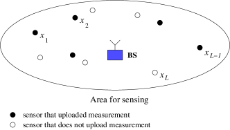
Figure 1: An illustration of an IoT system consisting of $L$ sensors and a BS.

If the BS can receive the measurements from all the sensors, it has the complete data set, ${\cal Y}$, that shall be available for a number of applications in IoT systems [3]. However, when $L$ is sufficiently large, with a limited bandwidth, it may take a long time to make ${\cal Y}$ available. As a result, when the uploading time is limited, it is desirable to find an estimate of ${\cal Y}$ using measurements from a small number of sensors. That is, as shown in Fig. 1, with a partial data set uploaded by a fraction of sensors (represented by black dots), the BS needs to perform interpolation to estimate the complete data set, ${\cal Y}$. Fortunately, provided that the measurements of closely located sensors are highly correlated, it is possible to have a good estimate of ${\cal Y}$ from measurements of a fraction of sensors using ML algorithms. Throughout the paper, we assume that the BS has sufficient computing power to perform ML algorithms. In this sense, the BS can also be seen as a server that performs ML algorithms to learn data sets.

II-B GPR

In this subsection, we present an overview of one of ML approaches, GPR [14], to learn data. Since GPR is a nonparametric regression approach, we will use it to estimate ${\cal Y}$ using a subset of ${\cal Y}$ without any specific parametric model.

Let ${\bf x}_{l}\in{\cal X}$ be the $l$th input location, where ${\cal X}$ represents the set of all possible locations (in the time or space domain). In addition, denote by $y({\bf x}_{l})$ the measurement or data at ${\bf x}_{l}$, i.e., $y_{l}=y({\bf x}_{l})$. It is assumed that

$$y({\bf x}_{l})\sim{\cal N}(m({\bf x}_{l}),\sigma^{2}),$$ (1)

where $m({\bf x}_{l})$ denotes the mean of the measurement at location ${\bf x}_{l}$ and $\sigma^{2}$ represents the variance of noisy observation. Furthermore, $m({\bf x})$ is assumed to be Gaussian that has the following distribution:

$$m({\bf x})\sim{\cal N}(0,k_{\theta}),$$ (2)

where $k_{\theta}$ represents the kernel that is parameterized by $\theta$ [14][15] [16].

Suppose that the measurements at certain locations, which are denoted by ${\bf x}_{1},\ldots,{\bf x}_{N}$, are available. That is, $y({\bf x})$ is available for ${\bf x}\in{\cal X}_{0}=\{{\bf x}_{1},\ldots,{\bf x}_{N}\}\subset{\cal X}$. For convenience, let ${\bf y}_{0}=[y({\bf x}_{1})\ \ldots\ y({\bf x}_{N})]^{\rm T}$. In addition, let ${\cal X}_{1}=\{{\bf x}_{N+1},\ldots,{\bf x}_{N+M}\}\subset{\cal X}$ be the test set, which is a set of certain locations of interest. Using GPR, although the measurements associated with ${\cal X}_{1}$ are not available, it is possible to find their estimates via the distribution of their mean values, which is the following conditional distribution:

$$f(m({\cal X}_{1})\,|\,{\bf y}_{0},{\cal X}_{0},{\cal X}_{1}),$$ (3)

where $m({\cal X}_{1})=[m({\bf x}_{N+1})\ \ldots\ m({\bf x}_{N+M})]^{\rm T}$. Under the Gaussian process assumption, the joint distribution of ${\bf y}_{0}$ and $m({\cal X}_{1})$ can be given by

$$\left[\begin{array}[]{c}{\bf y}_{0}\cr m({\cal X}_{1})\cr\end{array}\right]\sim{\cal N}\left({\bf 0},\left[\begin{array}[]{cc}{\bf K}_{\theta}({\cal X}_{0},{\cal X}_{0})+\sigma^{2}&{\bf K}_{\theta}({\cal X}_{0},{\cal X}_{1})\cr{\bf K}_{\theta}({\cal X}_{1},{\cal X}_{0})&{\bf K}_{\theta}({\cal X}_{1},{\cal X}_{1})\cr\end{array}\right]\right),$$ (4)

where ${\bf K}_{\theta}({\cal X}_{i},{\cal X}_{j})$ represents the covariance matrix comprising the covariance between an element of ${\cal X}_{i}$ and another element of ${\cal X}_{j}$, where $i,j\in\{0,1\}$. For example, $[{\bf K}_{\theta}({\cal X}_{0},{\cal X}_{1})]_{l,m}=k_{\theta}({\bf x}_{l},{\bf x}_{l+m})$, $l=1,\ldots,N$ and $m=1,\ldots,M$.

From (4), the conditional distribution of $m({\cal X}_{1})$, which is also Gaussian, has the mean and covariance matrix as follows:

$${\mathbb{E}}[m({\cal X}_{1})\,|\,{\bf y}_{0}] ={\bf K}_{\theta}({\cal X}_{1},{\cal X}_{0})\left({\bf K}_{\theta}({\cal X}_{0},{\cal X}_{0})+\sigma^{2}{\bf I}\right)^{-1}{\bf y}_{0}$$ (5)

$${\rm Cov}(m({\cal X}_{1})\,|\,{\bf y}_{0}) ={\bf K}_{\theta}({\cal X}_{1},{\cal X}_{1})-{\bf K}_{\theta}({\cal X}_{1},{\cal X}_{0})$$ (6)

$$\times\left({\bf K}_{\theta}({\cal X}_{0},{\cal X}_{0})+\sigma^{2}{\bf I}\right)^{-1}{\bf K}_{\theta}({\cal X}_{0},{\cal X}_{1}).$$ (7)

In (7), ${\mathbb{E}}[m({\cal X}_{1})\,|\,{\bf y}_{0}]$ can be seen as an estimate or prediction of the measurements of the sensors associated with ${\cal X}_{1}$ for given available measurements ${\bf y}_{0}$, and the conditional covariance matrix, ${\rm Cov}(m({\cal X}_{1})\,|\,{\bf y}_{0})$, can be used to see the estimation error or uncertainty of ${\mathbb{E}}[m({\cal X}_{1})\,|\,{\bf y}_{0}]$.

III Data-aided Sensing for GPR

Due to limited bandwidth for uplink transmissions, the BS may need to collect measurements from sensors through a number of rounds. Then, there can be a pre-determined order for sensors’ uploading, e.g., the increasing order in terms of the index, $l$. While any order can be considered, there could be a certain order that allows the BS to produce a good prediction of the values of the sensors that do not upload their measurements yet using the measurements from the sensors that already uploaded. The resulting approach is referred to as DAS in [12] [13]. In this section, DAS is applied to GPR where regression can be performed with active sensor selection so that a good estimate of the sensors’ complete data set, i.e., ${\cal Y}$, is available with a relatively small number of sensors.

For simplicity, suppose that one sensor can upload its measurement at each round. Denote by $l(t)$ the index of the sensor that uploads its measurement at round $t$, $t\geq 1$. In addition, let ${\cal L}(t)$ be the index set of the sensors that have uploaded their measurements up to round $t$, i.e., ${\cal L}(t)=\{l(1),\ldots,l(t)\}$. For convenience, let ${\cal L}(0)=\emptyset$. In addition, let

$${\bf y}(t)\!: {\cal L}(t)$$ the measurements corresponding to

$${\cal X}_{0}(t)\!: {\cal L}(t)$$ the set of locations of sensors corresponding to

$${\cal X}_{1}(t)\!: \ \mbox{the set of locations of sensors corresponding to ${\cal L}(t)^{c}$}.$$

Since ${\bf y}(t)\in{\mathbb{R}}^{t}$ becomes the vector of the measurements that are available at the BS up to round $t$, the BS can use GPR to find the conditional mean of $m({\cal X}_{1}(t))$ (for given ${\bf y}(t)$) as an estimate of the measurements of the sensors that do not upload yet (i.e., the sensors associated with ${\cal L}(t)^{c}$). That is, at round $t$, an estimate of the complete data set, ${\cal Y}$, can be obtained from the partial data set associated with ${\cal X}_{0}(t)$, i.e., ${\bf y}(t)$. The prediction for the measurements associated with ${\cal X}_{1}(t)$, ${\mathbb{E}}[m({\cal X}_{1}(t))\,|\,{\bf y}(t)]$, using GPR is given by

$$\hat{\cal Y}(t)=\left[\begin{array}[]{c}{\bf y}(t)\cr{\mathbb{E}}[m({\cal X}_{1}(t))\,|\,{\bf y}(t)]\cr\end{array}\right],$$ (8)

where $\hat{\cal Y}(t)$ denotes the estimate of ${\cal Y}$ at round $t$. The estimation error is dependent on the conditional covariance of $m({\cal X}_{1}(t))$, i.e., ${\rm Cov}(m({\cal X}_{1}(t)\,|\,{\bf y}(t))$. In particular, the mean squared error (MSE) of the estimate is given by

$${\mathbb{E}}[||m({\cal X}_{1}(t))-{\mathbb{E}}[m({\cal X}_{1}(t))\,|\,{\bf y}(t)]||^{2}]$$ (9)

$$\quad={\rm Tr}\left({\rm Cov}(m({\cal X}_{1}(t)\,|\,{\bf y}(t))\right).$$ (10)

At the next round, i.e., round $t+1$, a sensor can be selected by the BS to upload its measurement and the selection can be based on the minimization of MSE. To this end, with a certain $l\in{\cal L}(t)^{c}$, consider the joint distribution of ${\bf y}(t)$ and $m({\bf x}_{l})$ that has the following covariance matrix:

$${\rm Cov}\left(\left[\begin{array}[]{c}{\bf y}(t)\cr m({\bf x}_{l})\cr\end{array}\right]\right)=\left[\begin{array}[]{cc}{\bf K}_{\theta}({\cal X}_{0},{\cal X}_{0})+\sigma^{2}&{\bf k}_{\theta}({\cal X}_{0},{\bf x}_{l})\cr{\bf k}_{\theta}({\cal X}_{0},{\bf x}_{l})^{\rm T}&k_{\theta}({\bf x}_{l},{\bf x}_{l})\cr\end{array}\right].$$ (15)

Then, the conditional mean of $m({\bf x}_{l})$ for given ${\bf y}(t)$ becomes

$$m({\bf x}_{l}\,|\,{\bf y}(t))={\bf k}_{\theta}({\cal X}_{0},{\bf x}_{l})^{\rm T}\left({\bf K}_{\theta}({\cal X}_{0},{\cal X}_{0})+\sigma^{2}{\bf I}\right)^{-1}{\bf y}(t)$$ (16)

and the conditional variance is given by

$${\rm Cov}(m({\bf x}_{l}\,|\,{\bf y}(t)))=k_{\theta}({\bf x}_{l},{\bf x}_{l})$$ (17)

$$-{\bf k}_{\theta}({\cal X}_{0},{\bf x}_{l})^{\rm T}\left({\bf K}_{\theta}({\cal X}_{0},{\cal X}_{0})+\sigma^{2}{\bf I}\right)^{-1}{\bf k}_{\theta}({\cal X}_{0},{\bf x}_{l}).$$ (18)

Lemma 1.

Among all $l\in{\cal L}(t)^{c}$, the next sensor that can minimize the MSE of the estimate of $m({\cal X}_{1}(t))$ is the sensor associated with the maximum variance. As a result, the selection criterion to choose the next sensor in DAS is as follows:

$$l^{*}(t+1)=\operatorname*{\arg\!\max}_{l\in{\cal L}^{c}(t)}{\rm Cov}(m({\bf x}_{l}\,|\,{\bf y}(t))).$$ (19)

Proof:

The sum of the conditional variances of ${\bf x}_{l}$ for all $l\in{\cal L}(t)^{c}$ is also the MSE of the estimate of $m({\cal X}_{1}(t))$, $m({\cal X}_{1}(t)|{\bf y}(t))$, as follows:

$${\sf MSE}(t) ={\mathbb{E}}[||m({\cal X}_{1}(t))-{\mathbb{E}}[m({\cal X}_{1}(t)\,|\,{\bf y}(t)||^{2}]$$ (20)

$$=\sum_{l\in{\cal L}(t)^{c}}{\rm Cov}(m({\bf x}_{l}\,|\,{\bf y}(t))).$$ (21)

Suppose that $l\in{\cal L}(t)^{c}$ be the index of the next sensor so that ${\cal L}(t+1)=\{{\cal L}(t),l\}$ and ${\cal L}(t+1)^{c}={\cal L}(t)\setminus\{l\}$. Then, we have

$${\sf MSE}(t)={\rm Cov}(m({\bf x}_{l}\,|\,{\bf y}(t)))+\sum_{l^{\prime}\in{\cal L}(t)^{c}\setminus\{l\}}{\rm Cov}(m({\bf x}_{l^{\prime}}\,|\,{\bf y}(t))),$$

where the second term on the right-hand side becomes the MSE at round $t+1$. Since ${\sf MSE}(t)$ is independent of the selection of $l$, the minimization of the MSE at round $t+1$, i.e., $\min_{l}\sum_{l^{\prime}\in{\cal L}(t)^{c}\setminus\{l\}}{\rm Cov}(m({\bf x}_{l^{\prime}}\,|\,{\bf y}(t)))$, is equivalent to the maximization of ${\rm Cov}(m({\bf x}_{l}\,|\,{\bf y}(t)))$, i.e., $\max_{l}{\rm Cov}(m({\bf x}_{l}\,|\,{\bf y}(t)))$, which leads to the sensor selection criterion in (22) for DAS. ∎

Based on (22), DAS can be applied to GPR for a good estimate of the complete data set, ${\cal Y}$, with a small number of the sensors that upload their measurements. There are a few remarks as follows.

• We have assumed that ${\cal X}_{1}(t)$ is the set of the locations of the sensors that do not upload their measurements yet. It is also possible to define ${\cal X}_{1}(t)$ differently so that the measurements at locations without sensors can be estimated/predicted. In particular, suppose that it is required to interpolate virtual measurements at some locations’ where no sensors exist. Let $\tilde{\cal X}_{1}=\{\tilde{\bf x}_{1},\ldots,\tilde{\bf x}_{M}\}$, where $\tilde{\bf x}_{m}$ represents the $m$th location of interest with $\tilde{\bf x}_{m}\notin{\cal X}$. Then, DAS can be used for interpolation, and the next sensor to upload its measurement to minimize the MSE can be decided as follows:

  $$l^{*}(t+1)=\operatorname*{\arg\!\max}_{l\in{\cal L}^{c}(t)}{\rm Cov}(m(\tilde{\cal X}_{1})\,|\,{\bf y}(t),y({\bf x}_{l})).$$ (22)

  Note that the complexity of DAS is proportional to that of GPR as shown in (22), which is mainly dependent on the complexity of matrix inversion in (16) and (18) [14].

• Like Gaussian DAS in [13], (22) does not depend on the actual measurements, ${\cal Y}$, or available measurements, ${\bf y}(t)$. In other words, the order of sensors to upload does not depend on the existing data set, ${\bf y}(t)$. However, as will be shown in Section IV, there are also cases that the next sensor to upload its measurement depends on the existing data set or the current prediction of ${\cal Y}$.

• Although we only consider the case that all the measurements remain unchanged over a number of uploading rounds, they can be time-varying. Thus, to estimate ${\cal Y}$ within a limited time (for some real-time applications), DAS is more desirable to efficiently upload sensors’ measurements. DAS for time-varying models subject to delay constraints might be a further research topic to be investigated in the future.

IV Application-Dependent Criteria

In this section, we generalize DAS for active sensor selection to the case that multiple applications need an estimate of ${\cal Y}$ for different purposes.

Suppose that there are a number of different applications that use the measurements collected by the BS. Thus, the BS is to provide an estimate of ${\cal Y}$ using the measurements up to round $t$, ${\bf y}(t)$, i.e., $\hat{\cal Y}(t)$. Then, the conditional distribution of $\hat{\cal Y}(t)$ becomes

$$\hat{\cal Y}(t)\,|\,{\bf y}(t)\sim{\cal N}\left(\left[\begin{array}[]{c}{\bf y}(t)\cr m({\cal X}_{1}(t)\,|\,{\bf y}(t))\cr\end{array}\right],{\bf\Sigma}_{{\bf y}}(t)\right),$$ (23)

where

$${\bf\Sigma}_{{\bf y}}(t)=\left[\begin{array}[]{cc}{\bf 0}&{\bf 0}\cr{\bf 0}&{\rm Cov}(m({\cal X}_{1}(t))\,|\,{\bf y}(t))\cr\end{array}\right].$$ (24)

For example, suppose that $y_{l}=y({\bf x}_{l})$ is the temperature at a location of ${\bf x}_{l}$. Then, an application that is to provide the real-time mean temperature over the area where sensors are deployed can have the following estimate of the mean temperature:

$$\hat{\mu}(t)={\bf w}^{\rm T}\hat{\cal Y}(t),$$

where ${\bf w}=[\frac{1}{L}\ \ldots\ \frac{1}{L}]^{\rm T}$. In general, the output of an application can be given by

$$Z_{q}(t)={\bf w}_{q}^{\rm T}\hat{\cal Y}(t),$$ (25)

where ${\bf w}_{q}$ represents the weighting vector for the $q$th linear application. Here, by a linear application, we mean an application that provides an output as a linear function of $\hat{\cal Y}(t)$. For a linear application, the MSE of the output can be given by

$${\sf MSE}_{q}(t)={\bf w}_{q}^{\rm T}{\bf\Sigma}_{{\bf y}}(t){\bf w}_{q}.$$ (26)

Suppose that the $l$th sensor, $l\in{\cal L}(t)^{c}$, is chosen at round $t+1$. The conditional covariance matrix can be updated as follows:

$${\bf\Sigma}_{{\bf y},l}(t+1)=\left[\begin{array}[]{cc}{\bf 0}&{\bf 0}\cr{\bf 0}&{\rm Cov}(m({\cal X}_{1}(t))\,|\,{\bf y}(t),y({\bf x}_{l}))\cr\end{array}\right].$$ (27)

Then, for the $q$th application to minimize the MSE, the sensor to upload its measurement at round $t+1$ can be chosen as follows:

$$l_{q}(t+1)=\operatorname*{\arg\!\min}_{l\in{\cal L}(t)^{c}}{\sf MSE}_{q,l}(t+1),$$ (28)

where

$${\sf MSE}_{q,l}(t+1)={\bf w}_{q}^{\rm T}{\bf\Sigma}_{{\bf y},l}(t){\bf w}_{q}.$$ (29)

If there are $Q$ applications, there can be up to $Q$ different sensors that are to be selected at round $t+1$, i.e., $\{l_{1}(t+1),\ldots,l_{Q}(t+1)\}$. Alternatively, one sensor can be chosen at a time (or at each round) according to the weighted sum of MSEs as follows:

$$l(t+1)=\operatorname*{\arg\!\min}_{l\in{\cal L}(t)^{c}}\sum_{q}\beta_{q}{\sf MSE}_{q,l}(t+1),$$ (30)

where $\beta_{q}>0$ is the weight for the $q$th application.

There can be nonlinear applications. For example, if an application is to provide the maximum temperature over the area, the output is

$$Z=\max_{l}[\hat{\cal Y}(t)]_{l}.$$ (31)

Let $l^{*}(t)=\operatorname*{\arg\!\max}_{l}[\hat{\cal Y}(t)]_{l}$. If $l^{*}(t)\in{\cal L}(t)$, the maximum temperature is one of reported measurements up to round $t$. Otherwise, it becomes one of the predicted measurements of the sensors that do not upload yet. In this case, the application may wish to know its actual measurement. Thus, the index of the sensor at round $t+1$ can be given by $l(t+1)=l^{*}(t)\in{\cal L}(t)^{c}$.

Consequently, due to the presence of multiple applications (either linear or nonlinear applications), we can assume that there are multiple candidates sensors (say $Q$ sensors) to upload their measurements at each round. If the bandwidth of uplink channels is sufficiently wide, at each round, $Q$ different channels can be used to upload the measurements from $Q$ sensors simultaneously. However, if the bandwidth is limited, a fraction of $Q$ sensors may be able to send their measurements. In addition, there can be some sensors with their actual measurements that are sufficiently close to their predictions, in which case their uploading may result in waste of resource (i.e., uplink channels). In this case, the sensors may not need to upload their measurements. Thus, in DAS with multiple applications, it would be necessary to consider efficient uploading approaches due to limited bandwidth.

V Distributed Updating using Multichannel Random Access with Predictions

In this section, we study a distributed approach to upload sensors’ measurements using multichannel random access.

V-A Motivation

As discussed in Section IV, there can be $Q\ (\geq 1)$ sensors that are selected to upload their measurements at each round. Thus, for simultaneous uplink transmissions, multiple access channels can be used, say $B$ channels, where a sensor can upload its measurement through a dedicated channel at each round based on coordination by the BS (i.e., the BS can assign $B$ uplink channels to $B$ (out of $Q$) sensors). As a result, up to $B$ sensors can upload their measurements at each round. However, there can be some drawbacks as follows: i) some sensors may not have measurements due to various reasons (e.g., a sensor may be in dormant mode and so that it is unable to respond) [13]; ii) some sensors have measurements that are sufficiently close to their predictions at the BS and their uploading leads to waste of channel resource; iii) if $Q>B$, a single round is not sufficient. Thus, to address the those drawbacks, we consider a random access scheme, i.e., multichannel ALOHA with feedback of predictions, which will be discussed in the next subsection, rather than uploading coordinated by the BS.

Note that since multichannel ALOHA is employed for MTC [22][20] [23], DAS with multichannel ALOHA could be easily adopted with MTC in cellular IoT.

V-B Distributed Updating using Multichannel ALOHA

Suppose that there are $B$ multiple access channels for simultaneous uplink transmissions from multiple sensors. We assume that the BS can choose $Q$ sensors for uploading before round $t+1$, where $Q\geq B$. The index set of $Q$ sensors is denoted by

$${\cal L}_{Q}(t+1)=\{l_{1}(t+1),\ldots,l_{Q}(t+1)\},$$

where $l_{q}(t+1)$ represents the index of the $q$th candidate sensor at round $t+1$. Suppose that each of $Q$ sensors can decide whether or not it uploads its measurement independently with a certainly probability of uploading, which is denoted by $p_{\rm up}$. If a sensor decides to upload, which is referred to as an active sensor, it can choose one of $B$ channels uniformly at random. For convenience, let $K$ be the number of the sensors that decide to upload, which is a binomial random variable. Among $K$ active sensors, there can be multiple sensors that choose the same channel among $B$ channels, which results in collision. If collision happens, it is assumed that the BS cannot receive any measurements from the associated sensors. Since the probability that an active sensor can successfully transmit its measurement without collision is $\left(1-\frac{1}{B}\right)^{K-1}$, the average number of the sensors that can successfully upload their measurements without collisions is given by

$$S ={\mathbb{E}}\left[K\left(1-\frac{1}{B}\right)^{K-1}\right]$$ (32)

$$=\sum_{k=0}^{Q}k\left(1-\frac{1}{B}\right)^{k-1}\binom{Q}{k}p_{\rm up}^{k}(1-p_{\rm up})^{Q-k}.$$ (33)

After some manipulations, it can be shown that

$$S=p_{\rm up}Q\left(1-\frac{p_{\rm up}}{B}\right)^{Q-1}.$$ (34)

It is straightforward to show that $S$ is maximized when

$$p_{\rm up}=\frac{B}{Q}$$ (35)

and the maximum $S$ is

$$S_{\rm max}=B\left(1-\frac{1}{Q}\right)^{Q-1}\approx Be^{-1}.$$ (36)

Note that as mentioned earlier, suppose that some of sensors may not be able to upload their measurements with a probability of $p_{\rm sleep}$, In this case, for given $B$ channels, $Q$ can be decided as

$$Q=\frac{B}{1-p_{\rm sleep}},$$ (37)

so that the maximum $S$ can be achieved where $1-p_{\rm sleep}$ becomes effectively equal to the probability of uploading, $p_{\rm up}$.

Furthermore, as mentioned earlier, since the measurements of some of $Q$ sensors are close to predicted values by the BS, they may not need to upload. To modify multichannel ALOHA with the feedback of predictions, suppose that the BS can send the signals through downlink channel to the $Q$ candidate sensors with the predicted values of their measurements that are given by

$$m_{q}(t)=m({\bf x}_{q}\,|\,{\bf y}(t)),\ q\in{\cal L}_{Q}(t+1).$$ (38)

Then, at sensor $q\in{\cal L}_{Q}(t+1)$, with $m_{q}(t)$, the prediction error can be found as

$$e_{q}=m_{q}(t)-y({\bf x}_{q}).$$ (39)

For convenience, the sensor associated with $l_{q}(t+1)$ is referred to as the $q$th sensor in this section and omit the round index $t+1$. In addition, let $p_{q}$ be the probability of uploading of the $q$th sensor, which is now different for each sensor in the modified multichannel ALOHA. For given $p_{q}$, the $q$th sensor can generate a binary random variable, denoted by $V_{q}$, as follows:

$$V_{q}=\left\{\begin{array}[]{ll}1,&\mbox{w.p. $p_{q}$}\cr 0,&\mbox{w.p. $1-p_{q}$}\cr\end{array}\right.$$ (40)

If $V_{q}=1$, the $q$th sensor chooses one of $B$ channels uniformly at random and transmits its measurement as in conventional multichannel ALOHA [19] [20]. Otherwise, the $q$th sensor does not transmit.

Recall that $K$ is the number of active sensors, which can be written as

$$K=\sum_{q=1}^{Q}V_{q}\leq Q.$$ (41)

The probability that the $q$th sensor (regardless of its activity) eventually uploads its measurement can be given by

$$s_{q} =0\times\Pr(V_{q}=0)$$ (42)

$$\quad+{\mathbb{E}}\left[\left(1-\frac{1}{B}\right)^{K-1}\,|\,V_{q}=1\right]\times\Pr(V_{q}=1)$$ (43)

$$={\mathbb{E}}[V_{q}\psi_{B}^{\sum_{t\neq q}V_{t}}],$$ (44)

where $\psi_{B}=1-\frac{1}{B}$. Since the $V_{q}$’s are independent, we have

$$s_{q} ={\mathbb{E}}[V_{q}]{\mathbb{E}}[\psi_{B}^{\sum_{t\neq q}V_{t}}]=p_{q}{\mathbb{E}}[\prod_{t\neq q}\psi_{B}^{V_{t}}]$$ (45)

$$=p_{q}\prod_{t\neq q}{\mathbb{E}}[\psi_{B}^{V_{t}}]=p_{q}\prod_{t\neq q}(1-p_{t}+\psi_{B}p_{t})$$ (46)

$$={p_{q}}\prod_{t\neq q}\left(1-\frac{p_{t}}{B}\right).$$ (47)

From (47), we have $s_{q}\leq p_{q}$. In addition, if $B$ is sufficiently large, we can have

$$s_{q}=p_{q}\prod_{t\neq q}\left(1-\frac{p_{t}}{B}\right)\approx p_{q}e^{-\sum_{t\neq q}\frac{p_{t}}{B}}.$$ (48)

We can further show that

$$\sum_{q}s_{q} \approx\sum_{q}p_{q}e^{-\sum_{t\neq q}\frac{p_{t}}{B}}$$

$$\approx\sum_{q}p_{q}e^{-\frac{\sum_{t}p_{t}}{B}}=Pe^{-\frac{P}{B}}=B\frac{P}{B}e^{-\frac{P}{B}}\leq Be^{-1},$$

where $P=\sum_{q}p_{q}$. In general, $\sum_{q}s_{q}$ is maximized when $\sum_{q}p_{q}=B$. Furthermore, to minimize collisions, we can have the following constraint on $p_{q}$:

$$\sum_{q=1}^{Q}p_{q}\leq B.$$ (49)

At the BS, if sensor $q$ transmits without collision, the measurement error becomes 0. Otherwise, the measurement error is $m_{q}(t)-y({\bf x}_{q})$. Thus, the sum squared error (SSE) per round at the BS is

$${\sf SSE}=\sum_{q=1}^{Q}e_{q}^{2}(1-s_{q}),$$ (50)

which can be minimized by distributed selective uploading by $Q$ sensors that can decide $s_{q}$ or $p_{q}$ according to $e_{q}^{2}$. In (47), assuming that $\sum_{q}p_{q}\approx B$, we have $s_{q}\approx p_{q}e^{-1}$, and since $1-x<e^{-x}$ for a positive $x\ll 1$,

$${\sf SSE}\approx\sum_{q=1}^{Q}e_{q}^{2}(1-e^{-1}p_{q})\leq\sum_{q=1}^{Q}e_{q}^{2}\exp\left(-e^{-1}p_{q}\right).$$ (51)

Thus, to minimize the SSE, using the upper bound in (51), the following optimization can be considered:

$$\min_{\{p_{q}\}}\sum_{q=1}^{Q}e_{q}^{2}\exp\left(-e^{-1}p_{q}\right)$$ (52)

$$\mbox{subject to}\ \sum_{q=1}^{Q}p_{q}\leq B.$$ (53)

For a given Lagrange multiplier $\lambda$, each sensor can find $p_{q}$ that minimizes its cost function in a distributed manner as follows:

$$p_{q}(\lambda)=[e(\ln e_{q}^{2}-\psi)]_{0}^{1},$$ (54)

where $[x]_{a}^{b}=\min\{b,\max\{x,a\}\}$ for $b\geq a$ and $\psi=\ln(\lambda)+1$ (or $\lambda=e^{\psi-1}$). Clearly, (54) shows that the probability of uploading, $p_{q}$, can be decided at sensor $q$ provided that $\lambda$ is given.

At the BS, using dual ascent [24] $\psi$ can be updated as follows:

$$\psi(t+1)=\psi(t)+\mu\left(K(t)-B\right),$$ (55)

where $\mu>0$ is the step-size and $K(t)$ is the number of active devices at round $t$, which is an estimate of $\sum_{q}p_{q}$. Note that a similar distributed approach has been used for federated learning with multichannel ALOHA in [25]. Together with the feedback of predicted values, $\{m_{q}(t)\}$, the BS can also broadcast $\psi(t)$ so that the sensors can decide the probability of uploading according to (54). Note that at each round, since the SSEs are different, we cannot expect that $\psi(t)$ converges to a certain constant.

VI Numerical Results

In this section, we present numerical results to see the performance of GPR with DAS for different models for $\{{\bf x}_{l},y_{l}\}$. For simulations, the following kernel function is used

$$k_{\theta}({\bf x}_{l},{\bf x}_{l^{\prime}})=\exp\left(-\frac{1}{2}||{\bf x}_{l}-{\bf x}_{l^{\prime}}||^{2}\right).$$

VI-A Results for GPR with DAS

In this subsection, we present numerical results for GPR with random selection and DAS. Random selection is to choose one of the sensors associated with ${\cal X}_{1}(t)$ uniformly at random at each round. It is assumed that at each round, only one sensor uploads its measurement. To see how DAS works, only one run is considered with $L$ randomly located sensors and the performance measure is the MSE in (21). In addition, a sufficiently large $L$ is assumed so that the MSE after $L$ rounds can be sufficiently small (i.e., approaching 0).

As a toy example, we consider one-dimensional sensor network with $L=100$ sensors with

$$m(x)=\left(\sin\left(\frac{x}{3}\right)\right)^{2}-\frac{1}{5}\cos\left(\frac{x}{2}\right),\ 0\leq x\leq 10,$$ (56)

and

$$y_{l}=m(x_{l})+n_{l},$$

where $n_{l}\sim{\cal N}(0,\sigma^{2})$ is the noise. We assume that $x_{l}$ is random and uniformly distributed over $[0,10]$. As shown in Fig. 2, $m(x)$ over $x\in[0,10]$ is sufficiently smooth as the maximum frequency of $m(x)$ in (56) is $f_{\rm max}=\frac{1}{3\pi}\approx 0.1$. In Fig. 2, GPR results are shown with $L=100$ sensors and $\sigma^{2}=0.01$. In particular, Fig. 2 (a) shows that the MSE can rapidly decrease due to DAS compared to random selection. Thus, DAS allows GPR to provide a good estimate of the complete data set, ${\cal Y}$, with a small number of sensors uploading measurements (e.g., 20 sensors) compared to random selection, while DAS and random selection provide the same MSE after all the sensors upload their measurements. The positions of sensors that upload their measurements are shown in Fig. 2 (b) when random selection (on the left-hand side) and DAS (on the right-hand side) are used. Note that in Fig. 2 (b), the dashed line represents $m(x_{l})$, while the markers stand for actual noisy measurements at sensors. Clearly, we can see that the positions of uploaded sensors are more uniformly distributed by DAS than random selection, which leads to a better GPR performance using DAS (in terms of MSE as shown in Fig. 2 (a)).

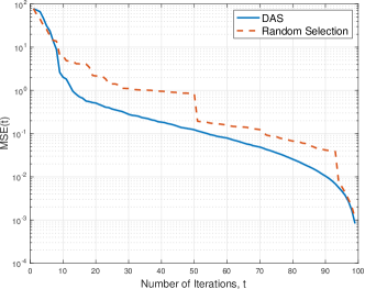
(a)

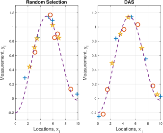
(b)

Figure 2: GPR results with $L=100$ and $\sigma^{2}=0.01$: (a) the MSEs as functions of round or iteration; (b) the uploaded measurements at the BS (the first 5 uploaded measurements are represented by $+$ markers, the next 5 by $\circ$ markers, and the next 5 by $\star$ markers.

For another toy example, consider a two-dimensional sensor network with the following $m({\bf x})$:

$$m({\bf x})=\frac{1}{3}\sum_{i=1}^{3}\exp\left(-({\bf x}-{\bf p}_{i})^{\rm T}{\bf A}_{i}({\bf x}-{\bf p}_{i})\right),\ {\bf x}\in[0,1]^{2},$$ (57)

where ${\bf p}_{1}=[0.1\ 0.9]^{\rm T}$, ${\bf p}_{2}=[0.5\ 0.6]^{\rm T}$, ${\bf p}_{3}=[0.9\ 0.7]^{\rm T}$, and

$${\bf A}_{1}=\left[\begin{array}[]{cc}4&-6\cr-1&6\cr\end{array}\right],{\bf A}_{2}=\left[\begin{array}[]{cc}8&1\cr 5&4\cr\end{array}\right],{\bf A}_{3}=\left[\begin{array}[]{cc}8&-4.1\cr-4.1&20\cr\end{array}\right].$$

Fig. 3 shows the performance of GPR with the 2-dimensional measurement model in (57) when $L=100$ and $\sigma^{2}=0.1$. To see the performance, $L=100$ locations are randomly generated within an area of $[0,1]^{2}$ for sensors (as shown by dots in Fig. 3 (b)). The MSEs as functions of iteration or round are shown in Fig. 3 (a), where GPR with DAS can decrease the MSE rapidly compared to GPR with random selection. In Fig. 3 (b), the positions of sensors that upload their measurements are shown. Clearly, DAS can allow GPR to take measurements from more uniformly located sensors and improve the performance of GPR. We also show the trace of the positions of uploaded sensors in a run in Fig. 3 (c), where the first sensor is shown by $\square$ marker. It is shown that any two consecutive sensors are not close to each other. This is due to the selection criterion in (22). That is, since the next sensor should have the largest covariance (or uncertainty) among those associated with ${\cal X}_{1}(t)$, any sensor that is close to the current one cannot be chosen as it may have a small (conditional) covariance.

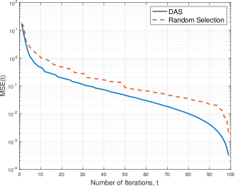
(a)

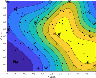
(b)

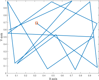
(c)

Figure 3: GPR results with $L=100$ and $\sigma^{2}=0.1$: (a) the MSEs as functions of round or iteration; (b) a 2-dimensional view of $m({\bf x})$ with the locations of sensors (represented by dots) and those of the sensors that uploaded measurements at the BS (the first 5 uploaded measurements are represented by $\square$ markers, the next 5 by $\circ$ markers, the next 5 by $\star$ markers, and the next 5 by $\triangleleft$ markers); (c) the trace of the first 15 uploaded sensors in a run (the $\square$ marker represents the first sensor).

The MSE curves in Figs. 2 – 3 are the outcomes for single realization of $L$ random locations. To see the average performance, we consider 1000 different realizations of $L$ locations, where $L=30$, and obtain the mean and standard deviation of MSEs. The mean MSE curves are shown with standard deviations in Fig. 4 with $\sigma^{2}=0.1$. It is clearly shown that DAS can provide not only a lower MSE, but also a smaller standard deviation than random selection.

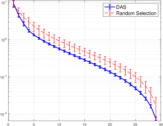
Figure 4: The mean and standard deviation of the MSEs with $L=30$ and $\sigma^{2}=0.1$. The vertical bars represent the standard deviations.

In Figs. 2 – 4, numerical results are provided with synthetic data sets. GPR with DAS can also be applied to real data sets. A data set of hourly measured ozone levels at 379 stations that is available from United State’s Environmental Protection Agency (EPA) is used. In Fig. 5 (a), the ozone levels (in parts per million (ppm)) at 379 locations are shown from the data set. The MSEs are shown in Fig. 5 (b), which demonstrates that GPR with DAS can decrease the MSE than GPR with random selection. In other words, DAS allows GPR to learn efficiently with fewer measurements than random selection. In particular, to achieve a target MSE of $10^{-2}$, DAS requires about 220 measurements, while random selection needs 350 measurements according to Fig. 5 (b). As a result, if there is a cost to obtain each measurement, DAS can help lower the cost in building a prediction model.

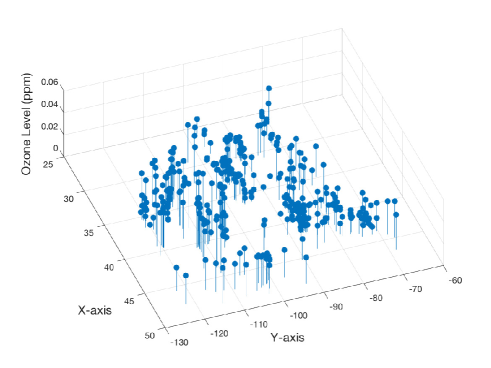
(a)

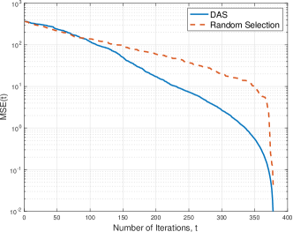
(b)

Figure 5: GPR results with the ozone levels at $L=379$ locations: (a) ozone levels in ppm at 379 locations; (b) the MSEs as functions of round or iteration.

VI-B Results with Multichannel ALOHA

In this subsection, we consider the case that $Q$ sensors are selected at each round with $B$ channels. Conventional multichannel ALOHA with an equal probability of uploading, $p_{\rm up}=\frac{B}{Q}$, is also considered to compare with the modified multichannel ALOHA where the predicted values of measurements are fed back to the $Q$ selected sensors. For simulations, the following 1-dimensional model is considered:

$$m(x)=\sqrt{\frac{2}{T}}\sum_{i=1}^{T}X_{i}\sin\left(2\pi f_{i}x+\theta_{i}\right),\ 0\leq x\leq 10,$$ (58)

where $X_{i}\sim{\cal N}(0,1)$, $f_{i}\sim{\rm Unif}(0,1/2)$, and $\theta_{i}\sim{\rm Unif}(0,2\pi)$. For all simulations, we assume that $T=10$ and in each run, $\{(X_{i},f_{i},\theta_{i})\}$ is randomly generated. Each simulation result is an average of 1000 runs.

To see the performance, the following SSE is used:

$${\sf SSE}({\cal U})=\sum_{q\in{\cal U}}e_{q}^{2},$$ (59)

where ${\cal U}$ represents the set of the sensors (among $Q$ selected sensors) that fail to upload their measurements due to collision. For convenience, at each round, $Q$ sensors are selected randomly rather than by any specific applications. Note that a lower-bound on the SSE can be obtained as follows:

$$\underline{{\sf SSE}}=\sigma^{2}(Q-Be^{-1}),$$ (60)

In (60), since $Be^{-1}$ is the average number of the sensors that successfully upload their measurement at each round (see (36)), $Q-Be^{-1}$ is the average number of the sensors that fail to upload. In (39), if the sensor’s prediction is perfect, ${\mathbb{E}}[e_{q}^{2}]$ becomes $\sigma^{2}$, which leads to the lower-bound in (60). That is, when GPR is able to perform good prediction with a sufficient number of measurements through a number of rounds, the lower-bound in (60) can be achieved.

Note that in the modified multichannel ALOHA with predictions, since sensors with large prediction errors have high probabilities of uploading, the sensors that do not upload more likely have low prediction errors. As a result, due to the (distributed) selective uploading, the SSE can be lower than that in (60) if the modified multichannel ALOHA with predictions is used.

Fig. 6 shows the SSE at each round with $L=200$, $Q=10$, $B=3$, and $\sigma^{2}=0.1$. For the case of conventional multichannel ALOHA, the equal probability of uploading, $p_{\rm up}=\frac{B}{Q}$, is used. On the other hand, in the modified multichannel ALOHA, $p_{q}$ is adaptively decided with predicted values when the step size is given by $\mu=0.5$. It is shown that GPR with conventional multichannel ALOHA can perform better than that with modified multichannel ALOHA up to 8 or 9 rounds, although modified multichannel ALOHA can provide a better performance than conventional multichannel ALOHA for GPR after 10 rounds. This is mainly due to the time to adjust the Lagrange multiplier through the adaptive algorithm in (55). It is also noteworthy that after a sufficient number of rounds, the SSE approaches the lower-bound in (60) as GPR can predict the measurements of the sensors that do not upload yet.

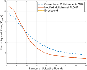
Figure 6: The SSEs of conventional multichannel ALOHA (with an equal probability of uploading, $\frac{B}{Q}$) and modified multichannel ALOHA with $p_{q}$ in (54) at each round with $L=200$, $Q=10$, $B=3$, and $\sigma^{2}=0.1$.

Fig. 7 shows the SSEs of conventional multichannel ALOHA (with an equal probability of uploading, $\frac{B}{Q}$) and modified multichannel ALOHA with $p_{q}$ in (54) after 40 rounds as functions of $B$ with $L=200$, $Q=10$, and $\sigma^{2}=0.1$. For a fixed $Q$, at each round, there are more sensors that succeed to upload their measurements for a larger $B$ (i.e., more channels), which leads to the decrease of SSE. With modified multichannel ALOHA, it is shown that $B=2$ or 3 channels are sufficient to approach the lower-bound on SSE. We also note that the SSE of modified multichannel ALOHA can be lower than the lower-bound on SSE, which was explained earlier due to the selective uploading.

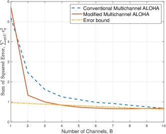
Figure 7: The SSEs of conventional multichannel ALOHA (with an equal probability of uploading, $\frac{B}{Q}$) and modified multichannel ALOHA with $p_{q}$ in (54) after 40 rounds as functions of $B$ with $L=200$, $Q=10$, and $\sigma^{2}=0.1$.

In Fig. 8, the SSEs of conventional multichannel ALOHA (with an equal probability of uploading, $\frac{B}{Q}$) and modified multichannel ALOHA with $p_{q}$ in (54) after 40 rounds are shown as functions of $Q$ with $L=200$, $B=4$, and $\sigma^{2}=0.1$. Since $B$ is fixed, it is shown that the SSE increases with $Q$. It is also observed that GPR with modified multichannel ALOHA outperforms GPR with conventional multichannel ALOHA for a wide range of $Q$.

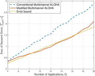
Figure 8: The SSEs of conventional multichannel ALOHA (with an equal probability of uploading, $\frac{B}{Q}$) and modified multichannel ALOHA with $p_{q}$ in (54) after 40 rounds as functions of $Q$ with $L=200$, $B=4$, and $\sigma^{2}=0.1$.

VII Concluding Remarks

In this paper, GPR has been considered for IoT systems to learn data sets collected from sensors without any specific model for data sets. To efficiently collect measurements from sensors, DAS was applied to GPR. In particular, we considered the interpolation of sensors’ measurements from a small number of measurements uploaded by a fraction of sensors. It was shown that GPR with DAS can have a good estimate of a complete data set using measurements uploaded by a fraction of sensors thanks to active sensor selection compared to GPR with random selection. As a result, when the number of sensors to upload their measurements is limited (due to various reasons including uploading time constraints), DAS can help GPR to efficiently learn data sets. DAS was also generalized with multichannel ALOHA where distributed selective uploading is employed, since each selected sensor can decide whether or not it uploads by comparing its measurement with the predicted one that is fed back by the BS.

The approach in this paper could be seen as an example to demonstrate how ML algorithms can learn data sets with efficient sensing and communication schemes (e.g., DAS). Thus, the approach can be extended for classification (when sensors’ measurements are to be labeled) and inference, which would be further research topics to be studied in the future.

References

- [1] J. Gubbi, R. Buyya, S. Marusic, and M. Palaniswami, “Internet of things (IoT): A vision, architectural elements, and future directions,” Future Gener. Comput. Syst., vol. 29, pp. 1645–1660, Sept. 2013.
- [2] J. Kim, J. Yun, S. Choi, D. N. Seed, G. Lu, M. Bauer, A. Al-Hezmi, K. Campowsky, and J. Song, “Standard-based IoT platforms interworking: implementation, experiences, and lessons learned,” IEEE Communications Magazine, vol. 54, pp. 48–54, July 2016.
- [3] A. Al-Fuqaha, M. Guizani, M. Mohammadi, M. Aledhari, and M. Ayyash, “Internet of Things: A survey on enabling technologies, protocols, and applications,” IEEE Communications Surveys Tutorials, vol. 17, pp. 2347–2376, Fourthquarter 2015.
- [4] I. Yaqoob, E. Ahmed, I. A. T. Hashem, A. I. A. Ahmed, A. Gani, M. Imran, and M. Guizani, “Internet of Things architecture: Recent advances, taxonomy, requirements, and open challenges,” IEEE Wireless Communications, vol. 24, no. 3, pp. 10–16, 2017.
- [5] J. Ding, M. Nemati, C. Ranaweera, and J. Choi, “IoT connectivity technologies and applications: A survey,” IEEE Access, vol. 8, pp. 67646–67673, 2020.
- [6] N. Mangalvedhe, R. Ratasuk, and A. Ghosh, “NB-IoT deployment study for low power wide area cellular IoT,” in 2016 IEEE 27th Annual International Symposium on Personal, Indoor, and Mobile Radio Communications (PIMRC), pp. 1–6, Sep. 2016.
- [7] 3GPP TS 36.321 V13.2.0, Evolved Universal Terrestrial Radio Access (E-UTRA); Medium Access Control (MAC) protocol specification, June 2016.
- [8] R. Soua and P. Minet, “A survey on energy efficient techniques in wireless sensor networks,” in 2011 4th Joint IFIP Wireless and Mobile Networking Conference (WMNC 2011), pp. 1–9, 2011.
- [9] C. S. Abella, S. Bonina, A. Cucuccio, S. D’Angelo, G. Giustolisi, A. D. Grasso, A. Imbruglia, G. S. Mauro, G. A. M. Nastasi, G. Palumbo, S. Pennisi, G. Sorbello, and A. Scuderi, “Autonomous energy-efficient wireless sensor network platform for home/office automation,” IEEE Sensors Journal, vol. 19, no. 9, pp. 3501–3512, 2019.
- [10] M. Z. A. Bhuiyan, G. Wang, J. Cao, and J. Wu, “Energy and bandwidth-efficient wireless sensor networks for monitoring high-frequency events,” in 2013 IEEE International Conference on Sensing, Communications and Networking (SECON), pp. 194–202, 2013.
- [11] C. Bockelmann, N. K. Pratas, G. Wunder, S. Saur, M. Navarro, D. Gregoratti, G. Vivier, E. De Carvalho, Y. Ji, C. Stefanović, P. Popovski, Q. Wang, M. Schellmann, E. Kosmatos, P. Demestichas, M. Raceala-Motoc, P. Jung, S. Stanczak, and A. Dekorsy, “Towards massive connectivity support for scalable mMTC communications in 5G networks,” IEEE Access, vol. 6, pp. 28969–28992, 2018.
- [12] J. Choi, “A cross-layer approach to data-aided sensing using compressive random access,” IEEE Internet of Things J., vol. 6, pp. 7093–7102, Aug 2019.
- [13] J. Choi, “Gaussian data-aided sensing with multichannel random access and model selection,” IEEE Internet of Things J., vol. 7, no. 3, pp. 2412–2420, 2020.
- [14] C. K. I. Williams and C. E. Rasmussen, “Gaussian processes for regression,” in Advances in Neural Information Processing Systems 8, pp. 514–520, MIT press, 1996.
- [15] C. E. Rasmussen and C. K. I. Williams, Gaussian Processes for Machine Learning. Cambridge, MA, USA: MIT Press, 2006.
- [16] C. M. Bishop, Pattern Recognition and Machine Learning. New York: Springer, 2006.
- [17] J. Wang, C. Jiang, H. Zhang, Y. Ren, K. C. Chen, and L. Hanzo, “Thirty years of machine learning: The road to Pareto-optimal wireless networks,” IEEE Communications Surveys Tutorials, vol. 22, no. 3, pp. 1472–1514, 2020.
- [18] D. A. Cohn, Z. Ghahramani, and M. I. Jordan, “Active learning with statistical models,” J. Artif. Int. Res., vol. 4, p. 129–145, Mar. 1996.
- [19] D. Shen and V. O. K. Li, “Performance analysis for a stabilized multi-channel slotted ALOHA algorithm,” in Proc. IEEE PIMRC, vol. 1, pp. 249–253 Vol.1, Sept 2003.
- [20] C. H. Chang and R. Y. Chang, “Design and analysis of multichannel slotted ALOHA for machine-to-machine communication,” in Proc. IEEE GLOBECOM, pp. 1–6, Dec 2015.
- [21] R. Jurdak, A. G. Ruzzelli, and G. M. P. O’Hare, “Radio sleep mode optimization in wireless sensor networks,” IEEE Trans. Mobile Computing, vol. 9, no. 7, pp. 955–968, 2010.
- [22] O. Galinina, A. Turlikov, S. Andreev, and Y. Koucheryavy, “Stabilizing multi-channel slotted ALOHA for machine-type communications,” in Proc. IEEE ISIT, pp. 2119–2123, July 2013.
- [23] J. Choi, “On the adaptive determination of the number of preambles in RACH for MTC,” IEEE Communications Letters, vol. 20, pp. 1385–1388, July 2016.
- [24] S. Boyd, N. Parikh, E. Chu, B. Peleato, and J. Eckstein, “Distributed optimization and statistical learning via the alternating direction method of multipliers,” Found. Trends Mach. Learn., vol. 3, pp. 1–122, Jan. 2011.
- [25] J. Choi and S. R. Pokhrel, “Federated learning with multichannel ALOHA,” IEEE Wireless Communications Letters, vol. 9, no. 4, pp. 499–502, 2020.