RACH in Self-Powered NB-IoT Networks: Energy Availability and Performance Evaluation

Abstract

NarrowBand-Internet of Things (NB-IoT) is a new 3GPP radio access technology designed to provide better coverage for a massive number of low-throughput low-cost devices in delay-tolerant applications with low power consumption. To provide reliable connections with extended coverage, a repetition transmission scheme is introduced to NB-IoT during both Random Access CHannel (RACH) procedure and data transmission procedure. To avoid the difficulty in replacing the battery for IoT devices, the energy harvesting is considered as a promising solution to support energy sustainability in the NB-IoT network. In this work, we analyze RACH success probability in a self-powered NB-IoT network taking into account the repeated preamble transmissions and collisions, where each IoT device with data is active when its battery energy is sufficient to support the transmission. We model the temporal dynamics of the energy level as a birth-death process, derive the energy availability of each IoT device, and examine its dependence on the energy storage capacity and the repetition value. We show that in certain scenarios, the energy availability remains unchanged despite randomness in the energy harvesting. We also derive the exact expression for the RACH success probability of a randomly chosen IoT device under the derived energy availability, which is validated under different repetition values via simulations. We show that the repetition scheme can efficiently improve the RACH success probability in a light traffic scenario, but only slightly improves that performance with very inefficient channel resource utilization in a heavy traffic scenario.

I Introduction

The Internet of Things (IoT) is a novel paradigm that is rapidly gaining interest in modern wireless telecommunications to support connections of billions of miscellaneous innovative devices. Third Generation Partnership Project (3GPP) has introduced several standards in its releases to improve support for Low Power Wide Area (LPWA) IoT connectivity [2, 3, 4]. In Rel-13, EC-GSM-IoT (Extended Coverage-GSM-IoT)[5] and LTE-MTC (LTE-Machine-Type-Communications)[6] have been introduced to existing Global System for Mobile Communications (GSM)[7] and Long-Term Evolution (LTE)[8] networks for better providing IoT devices, respectively. Another feature is NarrowBand-Internet of Things (NB-IoT)[5] whose applications include smart metering, intelligent environment monitoring, logistics tracking, municipal light, waste management, and so on.

I-A NarrowBand-Internet of Things

NB-IoT is a new 3GPP radio-access technology developed from existing LTE functionalities, whereas some features of its specification deemed unnecessary for LPWA IoT needs have been stripped out[9]. Because of this, NB-IoT can provide unique advantages for various IoT services over other technologies like 2G, 3G or LTE. LPWA networks mainly require deep/wide coverage, low power consumption, massive connections, and lower cost. The inherent characteristics of NB-IoT make it a good fit for LPWA deployment as shown in Fig. 1.

Figure 1: Main features of NB-IoT

Extending battery lifetime is one of the features of NB-IoT. There are several ways to reduce power consumption and achieve lifespans of IoT devices for more than 10 years. In the most simple way, we can switch the device to sleep mode when it does not work, so it doesn’t waste power while waiting. Power management is fundamentally the tradeoff between message frequency, device sleep cycles, and business case needs. Deep coverage is another feature of NB-IoT, where it is designed to improve indoor coverage by 20 dB compared to conventional GSM/GPRS. This is achieved by a higher power density, as radio transmissions are concentrated on a narrower carrier bandwidth of just 180 kHz. The Coverage Enhancement (CE) feature additionally offers the capability to repeat the transmission of a message when there exist poor coverage conditions but at the expense of a lower data rate.

NB-IoT reuses the LTE design extensively, such that the time required to develop full specifications and products is significantly reduced. In the downlink of NB-IoT, OFDMA (Orthogonal Frequency Division Multiplexing) technology is adopted with the sub-carrier spacing of 15 kHz and 12 sub-carriers make up the 180 kHz channel[10]. In the uplink, SC-FDMA (Single Carrier Frequency Division Multiple Access) technology including single sub-carrier and multiple sub-carrier are adopted. A single sub-carrier technology with 3.75 kHz and 15kHz is adopted with carrier spanning over 48 and 12 respectively. In this paper, we focus on NB-IoT Physical Random Access CHannel (NPRACH) with single sub-carrier spacing of 3.75 kHz.

NPRACH resources consist of the assignment of time and frequency resources and occur periodically. In the NPRACH, a random access preamble is transmitted which is the first step of random access procedure that enables the device to establish a data connection with its associated Evolved Node B (eNB)[10]. To improve the quality of service and reduce the power consumption of IoT devices, efficient RACH procedures need to be proposed and analyzed [9]. In [11, 12, 13], mathematical models of contention-based RACH focusing on the Signal-to-Interference-plus-Noise Ratio (SINR) outage or collision have been studied. However, to the best of our knowledge, most works have focused either on studying the SINR outage without considering collision or studying the collision from the single cell point of view and most results are based on the uplink power control due to its analysis simplicity.

Our previous work [14] has provided the preamble transmission model without considering the collision, [15] has considered the collision model without considering the repetition scheme, and [16] has considered the repetition scheme based on the uplink power control for simplicity. However, the IoT device adopts the cell specific maximum transmission power without power control when transmitting more than two preamble repetitions, which is motivated by the statement in 3GPP standard [5]. In this scenario, it is unknown 1) to what extent the transmission power affects the RACH success; 2) to what extent the repetition transmission scheme affects the RACH success; 3) how to choose the repetition value in different traffic scenarios to balance the RACH success probability and data transmission channel resources. To solve these problems, we present a novel mathematical framework to analyze and evaluate the RACH success probability, taking into account the SINR outage events as well as the collision events at the eNB, where the IoT devices adopt fixed transmission power.

Generally speaking, in the NB-IoT network, the physical layer parameters and network topology can strongly affect the RACH performance, due to that the received SINR at the eNB can be severely degraded by the mutual interference generated from massive IoT devices. In this scenario, the random positions of the transmitters make accurate modeling and analysis of this interference even more complicated. It is worth noting that stochastic geometry has been regarded as a powerful tool to model and analyze mutual interference between transceivers in the wireless networks[17], such as conventional cellular networks [18], wireless sensor networks [19], cognitive radio networks [20], and heterogenous cellular networks [21].

However, conventional stochastic geometry works [17, 18, 19, 20, 21] focused on analyzing normal uplink or downlink scheduled data transmission channel, where the intra-cell interference is not considered, due to the ideal assumption that each orthogonal sub-channel is not reused in a cell. The work [22] still focused on the scheduled data transmission, though it has considered the intra-cell interference over non-orthogonal sub-channels. All these stochastic geometry works are different from the RACH analysis in this paper, where massive IoT devices in a cell may randomly choose and transmit the same preamble to their associated eNB to request for channel resources for data transmission, and different preambles represent orthogonal sub-channels. Thus only IoT devices choosing the same preamble (i.e., sub-channel) have correlations. Note that IoT devices associated to the same eNB may choose the same preamble and collisions occur when two or more IoT devices transmit the same preamble simultaneously, such that the intra-cell interference and collisions are considered.

In practical NB-IoT networks, mutual interference among transmissions is much more intricate than the conventional LTE network systems. In this paper, we develop a novel mathematical framework for NB-IoT networks using stochastic geometry for RACH analysis with some challenges: 1) the distribution of the random transmission distances is considered, due to that the IoT device transmits with fixed transmission power; 2) the intra-cell interference is considered, due to that the massive IoT devices in a cell may randomly choose and transmit the same preamble using the same sub-channel; 3) the temporally correlated mutual interference is considered, due to that each IoT device remains spatially static during each repetition; 4) both the SINR outage and the collision events are considered, due to that collisions occur when two or more IoT devices transmit the same preamble simultaneously; 5) the network point of view analysis is considered instead of the single cell point of view, which is difficult in capturing both interference and collision generated from IoT devices transmitting with different transmit distances, due to the many concurrent transmissions and the interference experienced in each cell is different.

I-B Energy Harvesting

Human-operated cellular devices, such as smart phones, can be charged at will. But IoT devices are often located at remote and hard to reach locations, such as underground or in tunnels, without access power supply, which may be inconvenient, dangerous, expensive, or even impossible to change the battery. Hence, the battery energy storage highly determines the lifetime of the whole device, which provides a strong motivation for powering IoT devices by harvesting energy, such that networks consisting of energy harvesting or rechargeable batteries can survive perpetually[23]. Practically, energy can be harvested from renewable environmental sources including thermal, solar, wind, etc.[24] and radio signals of different frequencies such as radio broadcasting [25]. In these cases, the network performances are often tied closely to the efficiency in energy harvesting and utilization.

It is difficult to predict the time and the amount when the energy is available, as the energy arrival process is also random and dynamic. Energy buffer, i.e., battery storage, which collects harvested energy for signal processing and communication, is introduced in order to mitigate the unpredictability of the energy. Moreover, energy harvesting rates achievable today still fall short of typical power consumption levels. The harvested energy need to be accumulated in storage modules (e.g., capacitors or batteries) to a sufficient energy level to operate the IoT device. Nevertheless, the energy buffer is limited. It remains challenging to assign the amount of energy in terms of uncertain energy sources. To have an in-depth study on the harvesting and utilization of energy, we need an analytically simple yet practically accurate model of the harvested energy. Several models on the harvested energy have been used in literature, assuming a time-slotted system. The arriving of harvested energy is known as a deterministic way in[26] while unknown in[27]. In [28][29], the stationary Markovian models of the harvested energy were studied, which are analytically simple and are thus useful to provide insights for solving some key theoretical problems. However, the validity of these models has not been formally justified with empirical measurements, and hence it is not known if the insights are useful in practice. In [30], a more general analytical model for the harvested energy was provided with support from empirical measurements. In their empirical measurements, the harvested energy may be a Markovian process. In [31], sleep/wake-up strategies for various factors were studied, which determines the optimal parameters of the solar energy harvest based strategy using a bargaining game model. However, to the best of our knowledge, there has been no work studying energy harvesting in NB-IoT networks. In this work, we consider NB-IoT networks with the IoT devices harvesting energy from nature, e.g., solar cells, microbial fuel cells, and water mills, etc.

I-C Contributions and Outcomes

The contributions of this paper can be summarized as follows:

1) Using stochastic geometry, we present a tractable analytical framework for the self-powered NB-IoT network via energy harvesting from natural resources, in which the locations of the eNBs and the IoT devices are modeled as two independent Poisson Point Processes (PPPs) in the spatial domain.

2) We model the arrival of harvesting energy as independent Poisson arrival processes. Using tools from Markov stochastic process, we characterize the fraction of time each IoT device kept in ON state as the energy availability. We first model the temporal dynamics of the energy level as a birth-death process, and then derive the expression of energy availability of each IoT device using hitting time analysis.

3) Based on the derived energy availability of the IoT device, we drive the expression for the RACH transmission success probability of a randomly chosen IoT device with fixed transmission power under both SINR outage and collision conditions in the NB-IoT network. Furthermore, we develop a realistic simulation framework to capture the randomness locations, the preamble transmission as well as the RACH collision, and verify our derived RACH success probability.

4) Our results show that the energy availability of the IoT device increases at first and then remain unchanged, the RACH success probability increases, and the repetition efficiency decreases when increasing the repetition value. As such, the repetition value needs to be optimized. It is also noticed that in certain scenarios, the energy availability remains unchanged despite randomness in the energy harvesting. The results also show that there is an upper limit on transmission power and too large transmission power will waste energy.

The rest of the paper is organized as follows. Section II presents the network model. Section III derives energy availability of IoT device and analysis the actual result conditioning on some specific energy utilization strategies. Section IV derives the RACH transmission success probabilities of a randomly chosen IoT device. Section V presents the simulation framework. Finally, Section VI concludes the paper.

II System Model

II-A Network Description

We consider an uplink stochastic geometry model for NB-IoT system, consisting of a single class of eNBs and IoT devices, that are spatially distributed in the Euclidean plane $\mathbb{R}^{2}$ following two independent homogeneous Poisson Point Processes (PPPs) $\Phi_{\rm{B}}$ and $\Phi_{\rm{D}}$ with intensities $\lambda_{\rm{B}}$ and $\lambda_{\rm{D}}$, respectively. Without loss of generality, we assume each IoT device remains spatially static during time slots[16]. Same as [18], we assume that each IoT device associates with its geographically nearest eNB, where a Voronoi tesselation is formed. A standard power-law path-loss model is considered, where the path-loss attenuation is defined as $r^{-\alpha}$, with the propagation distance $r$ and the path-loss exponent ${\alpha}$. In addition, we consider a Rayleigh fading channel, where the channel power gain $h$ is assumed to be exponentially distributed random variable with unit mean, i.e., $h\sim$ Exp(1). All channel gains are assumed to be independent and identically distributed (i.i.d.) in space and time.

II-B Random Access Procedure

In the uplink of NB-IoT, data can only be transmitted via the dedicated uplink data transmission channel, Narrowband Physical Uplink Shared CHannels (NPUSCH), which is scheduled by the associated eNB. Before resource scheduling, the IoT device needs to execute a RACH to request uplink channel resources with the associated eNB. The RACH procedure of NB-IoT has the simplified message flow as for LTE, however, with different parameters[10]. There are two types of RACH procedures: contention-free and contention-based. The former is used to perform handover, whereas the latter is used otherwise [32]. The four-step contention-based RACH used by NB-IoT is described as follows.

In step 1, the device first transmits a preamble (msg1) on the NPRACH during the first Random Access Opportunity (RAO). The eNB periodically informs the devices about a set of up to 64 orthogonal preamble sequences from which the IoT device can make a choice. Collisions occur when two or more devices transmit the same preamble sequence simultaneously. In step 2, the IoT device sets a Random Access Response (RAR) window and waits for the eNB to transmit a RAR (msg2) with an uplink grant for the transmission of a message in the following step. If the device that sent a preamble sequence does not receive a msg2 from the eNB within a certain period of time, it enters a backoff period, trying to access the network once this period has expired. In step 3, the IoT device that successfully receives its RAR transmits a Radio Resource Control (RRC) Connection Request (msg3) with identity information to eNB. If two or more devices have chosen the same preamble sequence in a RAO, they will receive the same grant in the RAR message, and thus, their msg3 transmissions will collide. In step 4, the eNB transmits a RRC Connection Setup (msg4) to the IoT device when it successfully receives msg3. More details on the RACH can be found in [8][14].

Massive connections in NB-IoT make the simultaneous RACH requests under a limited number of available preambles one of the main challenges, thus we focus on the contention of preamble in step 1 of contention-based RACH, with the assumption that steps 2, 3, and 4 of RACH are always successful whenever step 1 is successful. If step 1 in RACH fails, i.e. the associated RAR message was not received, the IoT device needs to transmit another preamble in the next available RAO. That is to say, a RACH procedure is always successful if the IoT device successfully transmits the preamble to its associated eNB. In this case, the failure of this preamble transmission can result from the following two reasons: 1) the eNB cannot decode the preamble due to the low received SINR; 2) the eNB successfully decoded the same preamble from two or more IoT devices in the same time and causes the collision.

It is known that the collision event in step 1 of RACH can be detected by the eNB, when the collided IoT devices are separable in terms of the power delay profile [8]. Our model follows the assumption of collision handling in [15], where collision events are detected by eNB after it decodes the preambles in step 1 of RACH, and then no response will be fed back from the eNB to the IoT devices, such that it can not proceed to the next step of RACH [33].

II-C Narrowband Physical Random Access CHannel

NB-IoT technology occupies a frequency band of 180 kHz bandwidth[34], which corresponds to one resource block in LTE transmission. In the NPRACH, a preamble is transmitted based on symbol groups on a single subcarrier. A preamble consists of four symbol groups transmitted without gaps and can be repeated several times using the same transmission power. Frequency hopping is applied to symbol group granularity, i.e. each symbol group is transmitted on a different subcarrier. To serve UEs in different coverage classes, the NB-IoT network can configure up to 3 NPRACH resource configurations in a cell. In each configuration, a repetition value from the set $\{$1, 2, 4, 8, 16, 32, 64, 128$\}$ is specified for repeating a basic preamble[35]. In this model, we consider a single repetition value $N_{\rm{T}}$ as [16], where the channel resources assignment of NPRACHs only takes place at the beginning of each transmission time interval (TTI, i.e., a time slot) as shown in [16].

II-D Energy Harvesting Model

We assume that each IoT device is supported solely by the energy harvested from the surrounding environment (e.g., solar, kinetic, wind) and is equipped with a rechargeable battery with the finite capacity to buffer energy. Note that the assumption of a finite energy buffer is realistic since it is not possible to have infinite energy within an IoT device with limited physical dimensions. We model the energy arrival process of a randomly chosen IoT device in one TTI as an independent Poisson process with intensity $\mu_{0}$. This assumption is based on the fact that most energy harvesting modules contain small sub-modules harvesting energy independently, e.g., small solar cells harvesting energy in a solar panel, where the net energy harvested can be argued to be a Binomial process, which approaches to the Poisson process in the limit when the number of sub-modules grows large. This assumption is not uncommon, e.g., see [36][37].

Since the energy arrivals are random and the energy storage capacities are finite, there is some uncertainty associated with whether the IoT device has enough energy to serve itself at a particular time. Under such a constraint, the IoT device needs to be kept OFF, and be allowed to recharge before it has sufficient energy to serve itself in a given time slot. Thus, at any given time, an IoT device can be in either of the two operational states: ON or OFF. In this paper, the decision to toggle the operational state of an IoT device, i.e., turn ON or OFF, is taken by the device independently, and it is not influenced by the operational states of other IoT devices. For example, one IoT device may decide to turn OFF if its current energy level reaches below a certain predefined level, and to turn ON after harvesting enough energy over the other threshold.

We define the fraction of time that a randomly chosen IoT device remains ON as the $energy$ $availability$ $\eta_{0}$. In order to obtain $\eta_{0}$, we first need to characterize how the energy available at the IoT device changes over time. We model the available energy of an IoT device as a finite-state continuous-time Markov process (CTMC). In particular, let $\{M(t):t\geqslant 0\}$ be a stationary, homogeneous, and irreducible Markov process with state space $M=\{m_{1},m_{2},\cdots,m_{{i}}\}$ that specifies the energy state at time $t$. For this setup, we define the energy required of a randomly chosen IoT device in $each$ $repetition$ $E_{0}$ as the $unit$ $energy$[38]. Thus, the real energy state at a randomly chosen IoT device is directly proportional to the $E_{0}$ and the proportionality implies the maximum repetition value the IoT device can support. Without loss of generality, discretizing the real energy state of the IoT device by dividing by $E_{0}$, we get our state space of a randomly chosen IoT device as $M=\{0,1,\cdots,M_{0}\}$, in which $M_{0}=\bigl{\lfloor}{E}/{E_{0}}\bigr{\rfloor}$ and $E$ is the real energy storage capacity of the randomly chosen IoT device. Thus, the energy state $m\in M$ of the IoT device implies the maximum repetition value the IoT device can support with the energy. As such, the temporal dynamics of the battery energy levels can be modeled by the CTMC, in particular, the birth-death process illustrated in Fig. 2. When the IoT device is ON , the energy increases according to the energy harvesting rate $\mu_{0}$ units energy per second and decreases at a depletion rate of $\nu_{0}$ units energy per second.

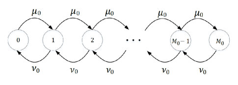
Figure 2: Birth-death process modeling the dynamics of the energy available at an IoT device

Note that the data transmission after a successful RACH can be extended following the analysis of RACH success probability. Since the main focus of this paper is analyzing the contention-based RACH in the NB-IoT network, we assume that the actual intended packet transmission is always successful (i.e., the data transmission success probability is one) if the corresponding RACH succeeds and that the RACH either always fails as shown in Fig. 3(a) or succeeds as shown in Fig. 3(b) to obtain the lower bound and upper bound of the $energy$ $availability$ $\eta_{0}$. Thus, we have $E_{0}^{f}$ = $E_{0}^{RA}$ for failure RACH and $E_{0}^{s}$ = $E_{0}^{RA}$ + $E_{0}^{DA}$ for successful RACH, where $E_{0}^{RA}$ is the energy required for the RACH in $each$ $repetition$; $E_{0}^{DA}$ is the energy required for the data transmission in $each$ $repetition$.

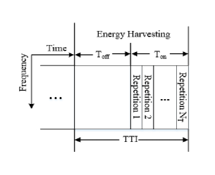
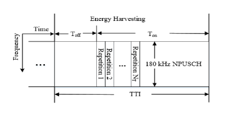
Figure 3: (a) Structure of failure NPRACH; (b) Structure of successful NPRACH and NPUSCH

Thus, we have incorporated the energy depletion rate for failure RACH and successful RACH cases separately as follows:

$$\begin{cases}{\nu_{0}}={\mathcal{A}_{a}}P/E_{0}^{f},&\mbox{if RACH fails},\\ {\nu_{0}}={\mathcal{A}_{a}}P/E_{0}^{s},&\mbox{if RACH succeeds},\end{cases}$$ (1)

where $P$ is the transmission power of each IoT device and $\mathcal{A}_{a}$ is the non-empty probability (i.e., IoT device data buffer is non-empty) described in Section IV.

The main notations of the proposed protocol are summarized in TABLE I.

TABLE I: Notation Table

$\lambda_{B}$	The intensity of BSs
$\lambda_{D}$	The intensity of IoT devices
$h$	The Rayleigh fading channel power gain
$r$	The distance between an IoT device and its associated BS
$\alpha$	The path-loss exponent
$N_{T}$	The RACH repetition value
$\mu_{0}$	The energy arrival rate
$E_{0}$	The energy required for each repetition
$E$	The real energy storage capacity
$\nu_{0}$	The energy depletion rate
$E_{0}^{RA}$	The energy required for the RACH in $each$ $repetition$
$E_{0}^{DA}$	The energy required for the data transmission in $each$ $repetition$
$\mathcal{A}_{a}$	The non-empty probability
$P$	The transmission power of each IoT device
$M_{0}^{c}$	The cutoff value
$M_{0}$	The storage capacity
$T_{0}^{\rm{off}}$	The time for which the IoT device remains in the OFF state
$T_{0}^{\rm{on}}$	The time for which the IoT device remains in the ON state
$\sigma^{2}$	The noise power
$\mathcal{I}_{0}$	The aggregate interference of the typical IoT device
$\mathcal{Z}_{D}$	The set of interfering IoT devices
$\gamma_{th}$	The SINR threshold
$L$	The number of available preambles are reserved for the contention-based RACH
${\lambda_{Da}}$	The density of active IoT devices choosing the same preamble
$c$	$c=3.575$ is a constant
$\eta_{0}$	The energy availability

III Energy Availability of IoT Devices

We assume that the energy harvesting processes are independent among the IoT devices, which ensure the independence of the current operational state (ON or OFF) of the IoT devices. An IoT device toggles its operational state solely on its current energy level. Essentially, we focus on a general strategy ${S\{M_{0}^{min},M_{0}^{c}\}}$ with energy storage capacity $M_{0}$ ($0\leq M_{0}^{min}\leq M_{0}^{c}\leq M_{0}$), where the randomly chosen IoT device toggles to OFF state when its energy level reaches below specific level $M_{0}^{min}$ and toggles back to ON state when its energy level reaches the predefined cutoff value $M_{0}^{c}$, i.e., it has sufficient energy to use. In addition, it should be noted that the cutoff value $M_{0}^{c}$ and $M_{0}^{min}$ can be defined and changed by the network if necessary.

We note that, it is strictly sub-optimal when the IoT device toggles to OFF at $M_{0}^{min}\neq 0$ for this model, since it effectively reduces the storage capacity from $M_{0}$ to $M_{0}-M_{0}^{min}$. That is to say, the strategy ${S_{1}\{M_{0}^{min},M_{0}^{c}\}}$ with energy storage capacity $M_{0}$ is equivalent to ${S_{2}\{0,M_{0}^{c}-M_{0}^{min}\}}$ with energy storage capacity ($M_{0}-M_{0}^{min}$), which are described in Table II.

TABLE II: Strategy Summary

${S_{1}}(M_{0}^{\min},M_{0}^{c})$	$M_{0}^{\min}$	$M_{0}^{c}$	$M_{0}$
${S_{2}}(0,M_{0}^{c}-M_{0}^{\min})$	0	$M_{0}^{c}-M_{0}^{\min}$	$M_{0}-M_{0}^{\min}$
${S_{3}}(M_{0}^{c}-{N_{T}},M_{0}^{c})$	$M_{0}^{c}-{N_{T}}$	$M_{0}^{c}$	$M_{0}$
${S_{4}}(0,{N_{T}})$	0	$N_{T}$	${M_{0}}$

In our work, the IoT device will be allowed to transmit only if it harvests sufficient energy for the transmission of at least $N_{T}$ times of repetitions. Then we set $M_{0}^{c}\geqslant N_{T}$ and $M_{0}^{min}=M_{0}^{c}-N_{T}\geqslant 0$, so we have our strategies as ${S_{3}\{M_{0}^{c}-N_{T},M_{0}^{c}\}}$ with energy storage capacity $M_{0}$. Therefore, without loss of generality, the strategies ${S_{3}\{M_{0}^{c}-N_{T},M_{0}^{c}\}}$ with energy storage capacity $M_{0}$ for our work is equivalent to ${S_{4}\{0,N_{T}\}}$ with energy storage capacity $M_{0}$. For the brevity of exposition, we denote this strategy by ${S\{N_{T}\}}$. In practical, the probability that the IoT device is available may be different for each device due to the differences in the capability $M_{0}$ of the energy harvesting modules and the repetition value $N_{T}$. However, we limit ourselves to the IoT device with the same repetition number $N_{T}$ and storage capability $M_{0}$ with the same energy availability probability.

For strategy ${S\{N_{T}\}}$, the time for which an IoT device remains in the ON state after it toggles from the OFF state is given by $T_{0}^{\rm{on}}\{N_{T}\}$, and the time for which it remains in the OFF state after toggling from the ON state is given by $T_{0}^{\rm{off}}\{N_{T}\}$. For notational simplicity, the cutoff value $\{N_{T}\}$ will be dropped wherever appropriate. It is noticed that both $T_{0}^{\rm{on}}$ and $T_{0}^{\rm{off}}$ are general random variables. We first obtain $T_{0}^{\rm{on}}$ as[39]

$${T_{0}^{\rm{on}}\{N_{T}\}=\inf\{\tau:{\xi_{0}}(\tau)=0|{\xi_{0}}(0)={N_{T}}\}},$$ (2)

where $\xi_{0}(\tau)$ denotes the current energy level of a randomly chosen IoT device at time $\tau$. For this setup, the energy availability of a randomly chosen IoT device depends only on the means of $T_{0}^{\rm{on}}$ and $T_{0}^{\rm{off}}$, which is shown as

$${\eta_{0}}=\displaystyle\frac{{{\mathbb{E}}[{T_{0}^{\rm{on}}}]}}{{{\mathbb{E}}[{T_{0}^{\rm{on}}}]+{\mathbb{E}}[{T_{0}^{\rm{off}}}]}}=\displaystyle\frac{1}{{1+{{{\mathbb{E}}[{T_{0}^{\rm{off}}}]}}/{{{\mathbb{E}}[{T_{0}^{\rm{on}}}]}}}},$$ (3)

and $\mathbb{E}$$[{T_{0}^{\rm{on}}}]$ is the mean time the randomly chosen IoT device remains in the ON state, and $\mathbb{E}$$[{T_{0}^{\rm{off}}}]$ is the mean time it remains in the OFF state.

Proof.

Let $\{T_{0}^{\rm{on}}(k)\}$ and $\{T_{0}^{\rm{off}}(k)\}$ be the sequences of the $k$th cycle of ON and OFF times, respectively. The availability can now be described by the fraction of time the randomly chosen IoT device remains in the ON state as

$${\eta_{0}}=\mathop{\lim}\limits_{K\to\infty}\displaystyle\frac{{\sum\nolimits_{k=1}^{K}T_{0}^{\rm{on}}(k)}}{{\sum\nolimits_{k=1}^{K}T_{0}^{\rm{on}}(k)+\sum\nolimits_{k=1}^{K}T_{0}^{\rm{off}}(k)}}.$$ (4)

Dividing both the numerator and the denominator by $K$ and invoking the law of large numbers, we have the result in (3).∎

Now we need to calculate the mean ON time $\mathbb{E}$$[{T_{0}^{\rm{on}}}]$ and the mean OFF time $\mathbb{E}$$[{T_{0}^{\rm{off}}}]$. For OFF time, according to [40], we have $\mathbb{E}[{T_{0}^{\rm{off}}}]={{{N_{T}}}}/{{{\mu_{0}}}}$ (i.e., the time required to harvest $N_{T}$ units of energy), which is the sum of $N_{T}$ exponentially distributed random variables, each with mean $1/\mu_{0}$. Substituting into (3), we obtain

$${\eta_{0}}=\displaystyle\frac{1}{{1+{{{N_{T}}}}/({{{\mu_{0}}{\mathbb{E}}[{T_{0}^{\rm{on}}}]}})}}.$$ (5)

To derive the mean ON time $\mathbb{E}[{T_{0}^{\rm{on}}}]$, we first need to obtain the transmission matrix $Q_{0}$ for the birth-death process corresponding to the randomly chosen IoT device. According to the Kolmogorov differential equations [41], $Q_{0}$=

$$\begin{bmatrix}-\mu_{0}&\mu_{0}&0&\cdots&0&0&0\\ \nu_{0}&-\mu_{0}-\nu_{0}&\mu_{0}&\cdots&0&0&0\\ 0&\nu_{0}&-\mu_{0}-\nu_{0}&\cdots&0&0&0\\ \vdots&\vdots&\vdots&\ddots&\vdots&\vdots&\vdots\\ 0&0&0&\cdots&{\nu_{0}}&-\mu_{0}-\nu_{0}&\mu_{0}\\ 0&0&0&\cdots&0&\nu_{0}&-{\nu_{0}}\end{bmatrix},$$ (6)

where the first column corresponds to the energy state 0 and the states are in the ascending order. Then we obtain the following Lemma 1. from [39].

Lemma 1.

(Mean Hitting Time). The expected hitting time of state $1$ (energy level $0$) starting from state m+$1$ (energy level m $\neq 0$) is

$${\mathbb{E}}[{T_{0}^{\rm{on}}}(m)]=\left({{{(-{{B}_{0}})}^{-1}}{\mathbbm{1}})}\right)(m),$$ (7)

where $B_{0}$ is a defined $M_{0}\times M_{0}$ matrix to be the restriction of matrix $Q_{0}$ to the set $M\setminus\{0\}$ i.e., $B_{0}=(Q_{0}(m,n),m\neq 0$, n $\neq 0)$, $-B_{0}$ is invertible and $\mathbbm{1}$ is a column vector of all $1$’s.

Now we can obtain a closed-form expression for the $(m,n)^{th}$ element in $(-B_{0})^{-1}$ by

$${(-{B_{0}})^{-1}}(m,n)=\frac{1}{{\nu_{0}^{n}}}\sum\limits_{k=1}^{\min(m,n)}{\mu_{0}^{n-k}}\nu_{0}^{k-1}.$$ (8)

Proof.

See Appendix A. ∎

Substituting (8) into (7) and then plugging into $m=N_{T}$, we have the mean ON time for strategy $S\{N_{T}\}$ with energy storage capacity $M_{0}$ as

$${\mathbb{E}}[T_{0}^{\rm{on}}({N_{T}})]$$ (9)

$$=\displaystyle\frac{{{{\Big{(}\displaystyle\frac{{{\mu_{0}}}}{{\nu_{0}}}\Big{)}}^{M_{0}+1}}\Big{(}{1-{{\Big{(}\displaystyle\frac{{{\mu_{0}}}}{{\nu_{0}}}\Big{)}}^{-{N_{T}}}}}\Big{)}}}{{\Big{(}{1-\displaystyle\frac{{{\mu_{0}}}}{{\nu_{0}}}}\Big{)}}}\displaystyle\frac{1}{{\nu_{0}-\mu_{0}}}-\frac{{{N_{T}}}}{{\mu_{0}-\nu_{0}}}.$$

Submitting (9) into (5), we obtain the energy availability in the following Theorem 1..

Theorem 1.

(Energy Availability). The energy availability of a randomly chosen IoT device is given by

$${\eta_{0}}=\displaystyle\frac{1}{{1+\displaystyle\frac{{{N_{T}}{{\Big{(}1-\displaystyle\frac{{{\mu_{0}}}}{{\nu_{0}}}\Big{)}}^{2}}}}{{{{\Big{(}\displaystyle\frac{{{\mu_{0}}}}{{\nu_{0}}}\Big{)}}^{{M_{0}}+2}}\Big{(}{1-{{\Big{(}\displaystyle\frac{{{\mu_{0}}}}{{\nu_{0}}}\Big{)}}^{-{N_{T}}}}}\Big{)}+\displaystyle\frac{{{\mu_{0}}}}{{\nu_{0}}}\Big{(}1-\displaystyle\frac{{{\mu_{0}}}}{{\nu_{0}}}\Big{)}{N_{T}}}}}}.$$ (10)

In (10), it can be shown that the energy availability increases with increasing $\mu_{0}$ and $M_{0}$. For illustration, the relationships between $\eta_{0}$ and $N_{T}$, $M_{0}$, $\mu_{0}$ are analyzed in Section V.

IV RACH Transmission Success Probability

In the NB-IoT repetition scheme, an active IoT device will repeat the same preamble $N_{T}$ times (i.e., the dedicated repetition value). In each repetition, a preamble is composed of four symbol groups transmitted without gaps, where the first preamble symbol group is transmitted via a sub-carrier determined by pseudo-random hopping (i.e., the hopping depends on the current repetition time and the Narrowband physical Cell ID, a.k.a NCellID[10]), and the following three preamble symbol groups are transmitted via sub-carriers determined by the fixed size frequency hopping[42]. This frequency hopping algorithm is designed in a way that different selections of the first subcarrier lead to hopping schemes which never overlap. Specifically, if two or more IoT devices chose the same first sub-carrier in a single RAO, the following sub-carriers (i.e., in the same RAO) would be same, due to that these two hopping algorithms lead to one-to-one correspondences between the first sub-carrier and the following sub-carriers (i.e., these IoT devices either collide on the full set or not collide at all in a single RAO). In this setup, the RACH success refers to the preamble being successfully transmitted to the associated eNB (i.e., received SINR is greater than the SINR threshold) and no collision occurs (i.e., no other IoT devices successfully transmit a same preamble to the typical eNB simultaneously).

For an IoT device to be able to initiate an uplink transmission, the energy harvested by this device should be sufficient to perform RACH and data transmission. We have defined the energy availability of a randomly chosen IoT device after harvesting enough energy as $\eta_{0}$ in Theorem 1. In this section, we first formulate the SINR outage condition to drive the preamble transmission success probability and then facilitate the analysis of the RACH success probability.

IV-A SINR Definition

Recall that each IoT device transmits a randomly chosen preamble to its associated eNB to request for channel resources, where different preambles represent orthogonal sub-channels, and thus only IoT devices choosing the same preamble have correlations. The RACH analysis in this work needs to take into account both the inter- and intra-cell interference. The received power at a typical eNB from a randomly chosen IoT device of interest is therefore $P_{0}=Ph_{0}r_{0}^{-\alpha}$, where $h_{0}$ and $r_{0}$ are the channel power gain and the distance from the typical IoT device to its associated eNB respectively. Using the received power over the link of interest and the interference power, the SINR received at the typical eNB at the origin can be written as

$${\rm{SINR}}({r_{0}})=\frac{{P{h_{0}}r_{0}^{-\alpha}}}{{\mathcal{I}_{0}^{{\mathop{intra}}}+\mathcal{I}_{0}^{{\mathop{inter}}}+{\sigma^{2}}}}=\frac{{P{h_{0}}r_{0}^{-\alpha}}}{{\mathcal{I}_{0}+{\sigma^{2}}}},$$ (11)

where $\sigma^{2}$ is noise power, and $\mathcal{I}_{0}$ is aggregate interference of the typical IoT device with

$$\mathcal{I}_{0}^{{\mathop{}}}=\sum\limits_{j\in{\mathcal{Z}_{{\mathop{D}}}}}{P{h_{j}}{r_{j}}^{-\alpha}}.$$ (12)

In (12), $h_{j}$ and $r_{j}$ are channel power gain and the distance from the interfering IoT devices to the typical eNB, $P$ is the transmission power of the IoT devices, and $\mathcal{Z}_{D}$ is the set of interfering IoT devices for the typical IoT device. We note that only the active IoT devices choosing the same preamble will generate interference. The density of active IoT devices choosing the same preamble is obtained as follows.

Remark 1.

(The density of active IoT devices choosing the same preamble). Note that inactive IoT devices (those without enough energy or data packets in buffer) do not attempt RACH, such that they do not generate interference. According to the repetition scheme mentioned earlier, each active IoT device will contend on all $L=48$ sub-carriers due to the single repetition value configuration, and thus each preamble has an equal probability $(1/L)$ to be chosen. As only active IoT devices will try to request uplink channel resources, we define the non-empty data packets probability of each IoT device $\mathcal{A}_{a}\in[0,1]$ following a Bernoulli process. We also have the energy availability $\eta_{0}$ of each IoT device, then according to the thinning process [44], the density of active IoT devices choosing the same preamble can be expressed as

$${\lambda_{Da}}=\mathcal{A}_{a}{\eta_{0}}{\lambda_{D}}/L.$$ (13)

IV-B RACH Success Probability

We formulate the RACH success probability under both SINR outage and collision conditions. We perform the analysis on an eNB associating with a randomly chosen active IoT device in terms of the RACH success probability. The RACH success refers to the preamble being successfully transmitted to the associated eNB (i.e., received SINR is greater than the SINR threshold) and no collision occurs (i.e., no other IoT devices successfully transmits a same preamble to the typical eNB simultaneously). First, we formulate the SINR outage condition. The typical IoT device transmits a preamble successfully if any repetition successes, and in a single repetition, a preamble is successfully received at the associated eNB if its all four received SINRs are above the SINR threshold $\gamma_{th}$. Thus, the preamble transmission success probability of a randomly chosen IoT device under $N_{T}$ repetitions is expressed as

$${{\mathbb{P}}_{S,0}}[{N_{T}}]=1-\underbrace{\prod\limits_{{n_{T}}=1}^{{N_{T}}}{\Big{(}{1-\underbrace{{{\mathbb{P}}_{0}}[{\theta_{{n_{T}}}}({r_{0}})|r_{0}]}_{\rm I}}\Big{)}}}_{{\rm I}{\rm I}}.$$ (14)

I is the probability that all four (a preamble consists of four preamble symbol groups) time-correlated preamble symbol groups in the $n_{T}$th repetition are successfully transmitted, II is the probability that all $N_{T}$ repetitions of a preamble transmission are failed, and

$${\theta_{{n_{T}}}}({r_{0}})=\big{\{} {\rm{SINR}}_{{n_{T}},1}({r_{0}})\geq{\gamma_{th}},{\rm{SINR}}_{{n_{T}},2}({r_{0}})\geq{\gamma_{th}},$$

$${\rm{SINR}}_{{n_{T}},3}({r_{0}})\geq{\gamma_{th}},{\rm{SINR}}_{{n_{T}},4}({r_{0}})\geq{\gamma_{th}}\big{\}}.$$ (15)

In (IV-B), $\gamma_{th}$ is the SINR threshold, and SINR${}_{{n_{T}},1}({r_{0}})$, SINR${}_{{n_{T}},2}({r_{0}})$, SINR${}_{{n_{T}},3}({r_{0}})$ and SINR${}_{{n_{T}},4}({r_{0}})$ are the received SINRs of the four symbol groups in the $n_{T}$th repetition of the typical IoT device. Based on the Binomial theorem, the preamble transmission success probability in (14) can be rewritten as

$${{\mathbb{P}}_{S,0}}[{N_{T}}]=$$

$$\sum\limits_{{n_{T}}=1}^{{N_{T}}}{{(-1)}^{{n_{T}}+1}}{\Big{(}\begin{array}[]{l}{N_{T}}\\ {n_{T}}\end{array}\Big{)}}{{\mathbb{P}}_{0}}[{\theta_{1}}({r_{0}}),{\theta_{2}}({r_{0}}),\cdots,{\theta_{{n_{T}}}}({r_{0}})|r_{0}],$$ (18)

where $\bigg{(}\begin{array}[]{l}{N_{T}}\\ {n_{T}}\end{array}\bigg{)}=\displaystyle\frac{{{N_{T}}!}}{{{n_{T}}!({{N_{T}}-{n_{T}}})!}}$ is the binomial coefficient, and $\displaystyle{{\mathbb{P}}_{0}[{\theta_{1}}({r_{0}}),{\theta_{2}}({r_{0}}),\cdots,{\theta_{{n_{T}}}({r_{0}})}]}$ is the probability that all of $4\times n_{T}$ (a preamble consists of four preamble symbol groups) time-correlated preamble symbol groups are successfully transmitted.

We note that the preamble transmission success probability in (IV-B) depends on the transmission distance $r_{0}$. Taking into account that each IoT device associates to its geographically nearest eNB, $r_{0}$ is the minimum distance between the eNB and the typical IoT device. The PDF of the shortest distance between any point BS and the IoT device with radius $r_{0}$ is [45]

$${f_{{R_{0}}}}({r_{0}})\approx 2\varepsilon\pi{\lambda_{B}}r_{0}\exp(-\varepsilon{\lambda_{B}}{\pi}r_{0}^{2}),$$ (19)

where $\varepsilon=1$ when $\lambda_{Da}\ll\lambda_{B}$ and $\varepsilon=1.25$ when $\lambda_{Da}\gg\lambda_{B}$.

For ease of presentation, we set $l=4\times n_{T}$, and the probability that all of $4\times n_{T}$ preamble symbol groups are successfully transmitted is presented in the following Lemma 2.

Lemma 2.

The probability that all of $4\times n_{T}$ received SINRs at the eNB from a randomly chosen IoT device exceed a certain threshold $\gamma_{th}$ is expressed as

$$p_{0}({\gamma_{th}})={\mathbb{E}_{{R_{0}}}}\Big{[}{\mathbb{P}}_{0}[{{\theta_{1}}(r_{0}),{\theta_{2}}(r_{0}),...,{\theta_{{n_{T}}}}(r_{0})|{{r_{0}}}}]\Big{]}$$

$$=\int{{\mathbb{P}}_{0}[{{\theta_{1}}(r_{0}),{\theta_{2}}(r_{0}),...,{\theta_{{n_{T}}}}(r_{0})|{{r_{0}}}}]}f(r_{0})d{r_{0}}$$

$$=\int_{0}^{\infty}{}2\varepsilon\pi{\lambda_{B}}r_{0}\exp\Big{(}-{\varepsilon\lambda_{B}}{\pi}r_{0}^{2}{{-\frac{{{l\gamma_{th}\sigma^{2}}r_{0}^{\alpha}}}{P}}}\Big{)}$$

$$\times\exp\Big{(}\overset{\text{}}{-2\pi{\lambda_{Da}}\int_{0}^{\infty}{\Big{[}{1-\big{(}{}{{1+{\gamma_{th}}r_{0}^{\alpha}{y^{-\alpha}}}}\big{)}^{-l}}\Big{]}}ydy}\Big{)}d{r_{0}}.$$ (20)

Proof.

See Appendix B. ∎

Next, we formulate the RACH success probability taking into account both the SINR outage and the collision. The RACH success probability is represented in the following Theorem 2.

Theorem 2.

In the energy harvesting NB-IoT network, the RACH success probability of a randomly chosen IoT device is derived as

$${{\cal P}_{0}} ={{\mathbb{E}}_{N}}{\Big{[}{{{{\mathbb{P}}_{S,0}}[{N_{T}}]}{\prod\limits_{j=1}^{n}{\Big{(}1-{{\mathbb{P}}_{S,j}}[{N_{T}}]\Big{)}}\Big{|}N=n}}\Big{]}}$$

$$=\sum\limits_{n=0}^{\infty}\Big{\{}\underbrace{{\mathbb{P}}[N=n]}_{{\rm I}}{{\underbrace{{{\mathbb{P}}_{S,0}}[{N_{T}}]}_{{\rm I}{\rm I}}\underbrace{\prod\limits_{j=1}^{n}{\Big{(}1-{{\mathbb{P}}_{S,j}}[{N_{T}}]\Big{)}}\Big{|}N=n}_{{\rm I}{\rm I}{\rm I}}}\Big{\}}},$$ (21)

where

$$\mathbb{P}[N=n]=\displaystyle\frac{{{c^{(c+1)}}\Gamma(n+c+1){{\big{(}{{{{\lambda_{Da}}}}/{{{\lambda_{B}}}}}\big{)}}^{n}}}}{{\Gamma(c+1)\Gamma(n+1){{\big{(}{{{{\lambda_{Da}}}}/{{{\lambda_{B}}}}+c}\big{)}}^{n+c+1}}}},$$ (22)

and

$${{{\mathbb{P}}_{S,0}}[{N_{T}}]}=\sum\limits_{{n_{T}}=1}^{{N_{T}}}{{(-1)}^{{n_{T}}+1}}{\Big{(}\begin{array}[]{l}{N_{T}}\\ {n_{T}}\end{array}\Big{)}}$$ (25)

$$\times\int_{0}^{\infty}{}2\varepsilon\pi{\lambda_{B}}r_{0}\exp\Big{(}-\varepsilon{\lambda_{B}}{\pi}r_{0}^{2}{{-\frac{{{l\gamma_{th}\sigma^{2}}r_{0}^{\alpha}}}{P}}}\Big{)}$$

$$\times\exp\Big{(}\overset{\text{}}{-2\pi{\lambda_{Da}}\int_{0}^{\infty}{\Big{[}{1-\big{(}{}{{1+{\gamma_{th}}r_{0}^{\alpha}{y^{-\alpha}}}}\big{)}^{-l}}\Big{]}}ydy}\Big{)}d{r_{0}}.$$ (26)

Part I the Probability Mass Function (PMF) of the number of intra-cell interfering IoT devices for a typical BS $N=n$ derived following [47, Eq.(3)], where $c=3.575$ is a constant related to the approximate PMF of the PPP Voronoi cell and $\Gamma(\cdot)$ is the gamma function. Part II is the preamble transmission success probability of a randomly chosen IoT device obtained by substituting (2) into (IV-B). Part III is the preamble transmission failure probability that the transmissions from other $n$ intra-cell interfering IoT devices are not successfully received by the BS, i.e., the non-collision probability of the typical IoT device conditioning on $n$.

Remark 2.

It is evident from (25) that the transmission success probability (II in (2)) of the typical IoT device increases, whereas the non-collision probability (III in (2)) decreases with increasing the repetition value $N_{T}$ and decreasing the the received SINR threshold $\gamma_{\rm th}$. Therefore, there exists a tradeoff between transmission success probability and non-collision probability. For illustration, the relationship among RACH access success probability $(\mathcal{P}_{0})$, the transmission success probability $(\mathcal{P}_{0}$ with III=1), and the non-collision probability $(\mathcal{P}_{0}$ with II=1) versus repetition value $N_{T}$ and the received SINR threshold $\gamma_{\rm th}$ is shown in Fig. 4.

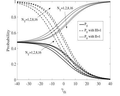
Figure 4: Comparing RACH access success probability (${\cal P}_{0}$), transmission success probability (${\cal P}_{0}$ with III = 1), and non-collision probability (${\cal P}_{0}$ with II = 1), $\lambda_{D}=10^{4}$ UEs/km².

Note that the RACH success probability of a randomly chosen IoT device in networks with perfect PRACH root sequence planning could be obtained by only considering the intra-cell interference. Considering that the practical Voronoi cells do not have a constant radius, we use the average radius $D=1/\sqrt{\pi{\lambda_{B}}}$[18] to approximate it. Thus, the RACH success probability is given in the following Lemma 3.

Lemma 3.

The RACH success probability of a randomly chosen IoT device in NB-IoT networks with perfect PRACH root sequence planning is derived as

$${{\cal P}_{0}} ={{\mathbb{E}}_{N}}{\Big{[}{{{{\mathbb{P}}_{S,0}}[{N_{T}}]}{\prod\limits_{j=1}^{n}{\Big{(}1-{{\mathbb{P}}_{S,j}}[{N_{T}}]\Big{)}}\Big{|}N=n}}\Big{]}}$$

$$=\sum\limits_{n=0}^{\infty}\Big{\{}\underbrace{{\mathbb{P}}[N=n]}_{{\rm I}}{{\underbrace{{{\mathbb{P}}_{S,0}}[{N_{T}}]}_{{\rm I}{\rm I}}\underbrace{\prod\limits_{j=1}^{n}{\Big{(}1-{{\mathbb{P}}_{S,j}}[{N_{T}}]\Big{)}}\Big{|}N=n}_{{\rm I}{\rm I}{\rm I}}}\Big{\}}},$$ (27)

where $\mathbb{P}[N=n]$ is given in (22) and

$${{{\mathbb{P}}_{S,0}}[{N_{T}}]}=\sum\limits_{{n_{T}}=1}^{{N_{T}}}{{(-1)}^{{n_{T}}+1}}{\Big{(}\begin{array}[]{l}{N_{T}}\\ {n_{T}}\end{array}\Big{)}}$$ (30)

$$\times\int_{0}^{\infty}{}2\varepsilon\pi{\lambda_{B}}r_{0}\exp\Big{(}-\varepsilon{\lambda_{B}}{\pi}r_{0}^{2}{{-\frac{{{l\gamma_{th}\sigma^{2}}r_{0}^{\alpha}}}{P}}}\Big{)}$$

$$\times\exp\Big{(}{-2\pi{\lambda_{Da}}\displaystyle\int_{0}^{\frac{1}{\sqrt{\pi{\lambda_{B}}}}}{\Big{[}{1-\Big{(}{}{{1+{\gamma_{th}}r_{0}^{\alpha}{y^{-\alpha}}}}\Big{)}^{-l}}\Big{]}}ydy}\Big{)}d{r_{0}}.$$ (31)

V Simulation and Discussion

In this section, we verify our analytical results by comparing the theoretical RACH success probabilities with the results from Monte-Carlo simulations. For numerical verification, we compute the RACH success probability from Monte-Carlo simulations as follows. We simulate the spatial model described in Section II in MATLAB. The eNBs and IoT devices are deployed via independent HPPPs in a $2\times 10^{4}$ km² circle area. Each IoT device associated with its nearest eNB. The IoT devices and the eNBs remain spatially static during a TTI. The channel fading gains between the IoT devices and eNBs are modeled by exponentially distributed random variables. Unless otherwise stated, we set $P=0.02$ w, $T_{r}=6$ ms, $T_{g}=31$ ms, $\mu_{i}=0.05$, $\lambda_{\rm{B}}=0.1$ eNBs/km², $\lambda_{\rm{D}}=10^{2}$ IoT devices/km², $\gamma_{th}=20$ dB, $\alpha=4$, $\mathcal{A}_{a}=0.001$, the bandwidth of a subcarrier is BW$=3.75$ kHz, and thus the noise is $\sigma^{2}=−174+10$log$10$(BW) $=−138.3$ dBm. For each realization of this setup, the uplink communication has declared a success if 1) the calculated SINR exceeds a pre-determined threshold $\gamma_{th}$ and 2) other uplink communications using the same preamble do not exceed $\gamma_{th}$. In all figures of this section, “Analytical” and “Simulation” are abbreviated as “Ana.” and “Sim.”, respectively.

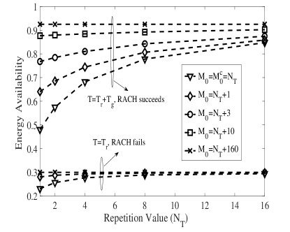
Figure 5: The energy availability of the IoT device for $S\{N_{T}\}$ versus the repetition value $N_{T}$ for various storage capacities ${M_{0}}$.

V-A Analysis of the Energy Availability

Fig. 5 plots the energy availability of a randomly chosen IoT device under our strategy $S\{N_{T}\}$ versus the preamble repetition value $N_{T}$ for various storage capacities ${M_{0}}$ using (10). We assume that the RACH in each TTI succeeds or fails on the full set (i.e., the RACH always succeeds or all the RACH always fails), and then we derive the upper bound and the lower bound of the energy availability. As such, we could give the availability region for various values of energy availability.

We first observe that the energy availability of the IoT device increases with increasing the preamble repetition value $N_{T}$ at first and then remains unchanged. This is due to the fact that for the same storage capacity, increasing the repetition value increases the operation time of the IoT device, i.e., the IoT device spends more time in ON state. In addition, since ${M_{0}^{c}}=N_{T}$, increasing the repetition value $N_{T}$, i.e., increasing the cutoff value, results in more time needed for the IoT device to harvest sufficient energy, i.e, stay in OFF state for more time before the transmission. As such, to obtain a higher energy availability, a larger repetition value $N_{T}$ is needed, but if the repetition value is overestimated, the IoT device will waste the potential resource for data transmission and lead to lower resource efficiency. That is to say, the repetition value needs to be optimized. Interestingly, we also observe that for energy storage capacity much larger than cutoff value, the energy availability approaches a specific value for different preamble repetition values, e.g., $\eta_{0}=0.3$ for the lower bound when and $\eta_{0}=0.92$ for the upper bound when $M_{0}-{M_{0}^{c}}\geq 160$, which reveals that this setup is surprisingly reliable if it is designed properly, despite the randomness in the energy harvesting.

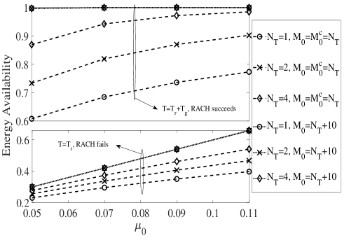
Figure 6: The energy availability of the IoT device for $S\{N_{T}\}$ versus the energy harvesting rate $\mu_{0}$ for various storage capacities ${M_{0}}$ and repetition values $N_{T}$.

Fig. 6 plots the energy availability of the randomly chosen IoT device under our strategy $S\{N_{T}\}$ versus the energy harvesting rate $\mu_{0}$ for various storage capacities ${M_{0}}$ and repetition values $N_{T}$ using (10). We first observe that the energy availability of the IoT device increases with increasing the energy harvesting rate $\mu_{0}$ when the storage capacity $M_{0}$ is not large enough, e.g.,$M_{0}=N_{T}$. This is due to the fact that for the same storage capacity and the cutoff value, increasing the energy harvesting rate results in less time needed for the IoT device to harvest sufficient energy, i.e, stay in OFF state for less time before the transmission. Interestingly, we also observe that for energy storage much larger than cutoff value, e.g., $M_{0}-M_{0}^{c}\geq 10$, the energy availability approaches a specific value for different preamble repetition values. That is to say, if it is designed properly, the energy availability is independent of $N_{T}$.

V-B Validation of the RACH success probability

In this section, we simulate an NB-IoT network and evaluate the RACH success probability based on the energy availability analyzed above. Fig. 7 plots the RACH success probability of a randomly chosen IoT device versus the energy availability $\eta$ for various preamble repetition values $N_{T}$. We observe that the RACH success probability deteriorates as the energy availability of IoT devices increases. This is due to the fact that increasing energy availability increases the number of active devices, which leads to lower received SINR and a higher probability of collision. In order to obtain fundamental insights on the RACH success probability due to the preamble repetition value $N_{T}$, in the following analysis, we use unchanged $\eta_{0}=0.3$ for different $N_{T}=$1, 2, 4, and 8, which is obtained by fine tuning $M_{0}-{M_{0}^{c}}\geq 160$ as shown in Fig. 5.

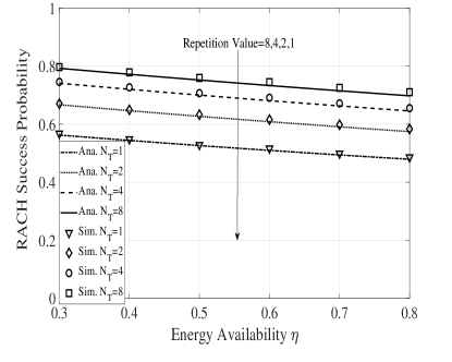
Figure 7: RACH success probability versus the energy availability $\eta_{0}$ for various repetition values $N_{T}$.

Fig. 8 plots the RACH success probability of a randomly chosen IoT device versus the transmission power $P$ for various preamble repetition values $N_{T}$. We first observe a good match between the analysis and the simulation results, which validates the accuracy of the developed mathematical framework. As expected, we observe that the RACH success probability increases as the transmission power of IoT devices increase. This can be explained by the reason that whilst increasing the transmission power $P$ leads to higher interference power, it also leads to increased received signal power, thereby improves the overall SIR and hence the RACH success probability. It is worth noting that the RACH success probability increases faster at first (e.g., when $P\leq 0.1$) and then gradually becomes steady, which reveals that there is a limit value of the cell maximum transmission power. Interestingly, we observe that the RACH success probabilities with a higher repetition value, e.g., $N_{T}=8$ become stable earlier than those with a lower repetition value, e.g., $N_{T}=1$, due to that the higher chance of the RACH to succeeds in higher repetition value case.

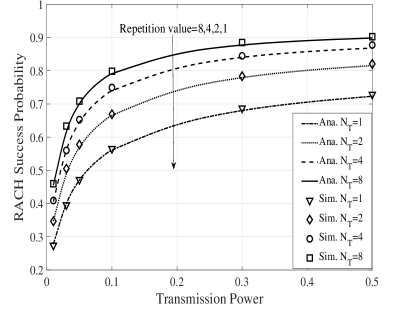
Figure 8: RACH success probability versus the transmission powers $P$ for various repetition values $N_{T}$.

Fig. 9 plots the RACH success probability of a randomly chosen IoT device versus the SINR threshold $\gamma_{th}$ for various preamble repetition values $N_{T}$. As expected, the RACH success probability degrades with an increase in the SINR threshold. According to Fig. 4, increasing SINR threshold $\gamma_{th}$ leads to lower preamble transmission success probability but higher non-collision probability, thereby decreases the overall RACH success probability. There is a tradeoff between preamble transmission success probability and non-collision probability.

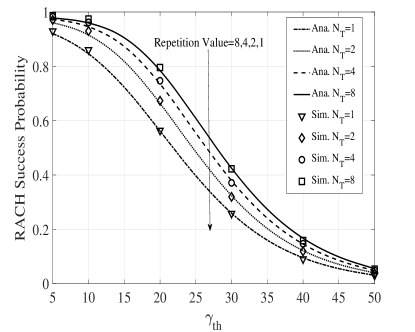
Figure 9: RACH success probability versus the SINR threshold $\gamma_{th}$ for various repetition values $N_{T}$.

Fig. 10(a) and Fig. 10(b) plot the RACH success probability of a randomly chosen IoT device versus the density ratio $\lambda_{D}/\lambda_{B}$ in the network with and without inter-cell interference, respectively. We first observe that the RACH success probability decreases with the increase of the density ratio between IoT devices and BSs ($\lambda_{D}/\lambda_{B}$), which is due to the following two reasons: 1) increasing the number of IoT devices generating interference leads to lower received SINR at the eNB; 2) increasing the number of IoT devices leads to higher probability of collision. In addition, increasing repetition value increases the RACH success probability due to that it offers more opportunities to re-transmit a preamble with the time and frequency diversity.

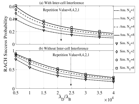
Figure 10: RACH success probability versus density ratio $\lambda_{D}/\lambda_{B}$ in the network with and without inter-cell interference.

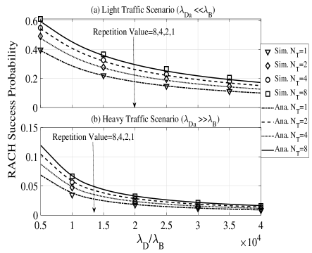
Figure 11: RACH success probability versus density ratio $\lambda_{D}/\lambda_{B}$ in the network with light traffic and heavy traffic.

Fig. 11(a) and Fig. 11(b) plot the RACH success probability of a randomly chosen IoT device versus the density ratio $\lambda_{D}/\lambda_{B}$ in the network with light traffic ($\mathcal{A}_{a}=0.001$, $\lambda_{Da}\ll\lambda_{B}$, and $\varepsilon=1$) and heavy traffic ($\mathcal{A}_{a}=0.015$, $\lambda_{Da}\gg\lambda_{B}$, and $\varepsilon=1.25$), respectively. In the light traffic scenario, RACH success probability increase when increasing the repetition value. However, in the heavy traffic scenario, the RACH success probability cannot improve much when the repetition value increased. That is to say, the repetition scheme can efficiently improve the RACH success probability in a light traffic scenario, but only slightly improves that performance with very inefficient channel resource utilization in a heavy traffic scenario.

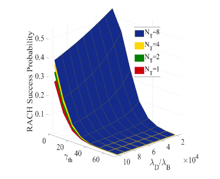
Figure 12: RACH success probability of a randomly chosen IoT device versus the densities ratio $\lambda_{D}/\lambda_{B}$ and SINR threshold $\gamma_{th}$.

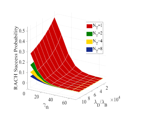
Figure 13: Repetition efficiency of a randomly chosen IoT device versus the densities ratio $\lambda_{D}/\lambda_{B}$ and SINR threshold $\gamma_{th}$.

Fig. 12 and Fig. 13 plot the RACH success probability and the Repetition efficiency (i.e., $\zeta={{\cal P}_{0}}/{N_{T}}$) of a randomly chosen IoT device versus the density ratio $\lambda_{D}/\lambda_{B}$ and SINR thresholds $\gamma_{th}$, respectively. Obviously, increasing the repetition value increases the success opportunities of RACH, but decreases the repetition efficiency, which reveals that if the repetition value is overestimated, the IoT device will waste the potential resource for data transmission and lead to lower resource efficiency. In addition, we observe that the repetition efficiencies decrease seriously when increasing the repetition value from $N_{T}=1$ to $N_{T}=2$, especially for the lower density ratio. This is due to the fact that when there are fewer active IoT devices (e.g., $\lambda_{D}/\lambda_{B}=10^{4}$) to contention for the same resources, it is likely to succeed with small repetition values, which contributes to a relatively high channel resource utilization.

VI Conclusion

In this paper, we have presented a comprehensive RACH success probability analysis for the NB-IoT network with energy harvesting from natural resources. We have derived a closed-form expression of the energy availability and analyzed the results for some realistic strategies. We found that energy availability remains unchanged if the network is properly designed despite randomness in energy harvesting. We further analyzed the RACH under the repetition transmission scheme in the NB-IoT system based on energy availability. We derived the exact expression for the RACH success probability under time-correlated interference. Different from existing works, we considered both SINR outage and collision from the network point of view in the NB-IoT network, where each IoT device adopts fixed transmission power. Our results have shown that increasing the repetition value increases the RACH success probability but decreases the repetition efficiency. In the light traffic scenario, RACH success probability can meet the requirement with small repetition values. However, in the heavy traffic scenario, very high repetition value leads to a low channel resources utilization. Our results also have shown that there is an upper limit on transmission power and too large transmission power will waste energy.

Appendix A a proof of lemma 1

Let $A_{0}=-B_{0}$ and then we have

$$A_{0}{A_{0}}^{-1}=I,$$ (A.1)

where ${A_{0}}^{-1}$ is the inverse of the matrix ${A_{0}}$. Let

$${A_{0}}^{-1}=(a_{mn})_{1\leq m,n\leq M_{0}}=(A_{1},A_{2},\cdots,A_{M_{0}}),$$ (A.2)

and

$$I=(e_{mn})_{1\leq m,n\leq M_{0}}=(E_{1},E_{2},\cdots,E_{M_{0}}),$$ (A.3)

where $A_{r}$ and $E_{r}$ denote the $r$th column of ${A_{0}}^{-1}$ and $I$ respectively, $r=1,2,\cdots,M_{0}$. Then (A.1) can be rewritten in the form

$$A_{0}A_{r}=E_{r}.$$ (A.4)

In order to calculate ${A_{0}}^{-1}$, we begin by considering the elements of the first column $A_{1}=(a_{11},a_{21},\cdots,a_{M_{0}1})^{T}$ of ${A_{0}}^{-1}$. That means

$$\begin{bmatrix}\mu_{0}+\nu_{0}&-\mu_{0}&0&\cdots&0&0\\ -\nu_{0}&\mu_{0}+\nu_{0}&-\mu_{0}&\cdots&0&0\\ \vdots&\vdots&\vdots&\ddots&\vdots&\vdots\\ 0&0&0&\cdots&{\mu_{0}}+{\nu_{0}}&-\mu_{0}\\ 0&0&0&\cdots&-\nu_{0}&\nu_{0}\end{bmatrix}\begin{bmatrix}{a_{1{1}}}\\ {a_{2{1}}}\\ \vdots\\ {a_{{M_{0-1}}{1}}}\\ {a_{{M_{0}}{1}}}\end{bmatrix}$$

$$=\begin{bmatrix}1&0&\cdots&0&0\end{bmatrix}^{T}.$$ (A.5)

Then we have $A_{1}$=$(1/\nu_{0},1/\nu_{0},\cdots,1/\nu_{0})^{T}$. Plugging $r=2,3,\cdots,M_{0}$ into (A.4) respectively, we have all the elements of ${A_{0}}^{-1}$, i.e, $(-{B_{0}})^{-1}$.

Appendix B a proof of lemma 2

We note that the preamble transmission success probability in (IV-B) depends on the transmission distance $r_{0}$. According to the PDF of $r_{0}$ given in (19), we have

$$p_{i}({\gamma_{th}})={\mathbb{E}_{{R_{0}}}}\Big{[}{\mathbb{P}}_{0}[{{\theta_{1}}(r_{0}),{\theta_{2}}(r_{0}),...,{\theta_{{n_{T}}}}(r_{0})|{{r_{0}}}}]\Big{]}$$

$$=\int{{\mathbb{P}}_{0}[{{\theta_{1}}(r_{0}),{\theta_{2}}(r_{0}),...,{\theta_{{n_{T}}}}(r_{0})|{{r_{0}}}}]}f(r_{0})d{r_{0}}$$

$$=\int{{\mathbb{P}}_{0}}[{\rm SINR_{1}}({r_{0}})\geqslant{\gamma_{th}},\cdots,{{\rm SINR}_{l}}({r_{0}})\geqslant{\gamma_{th}}\big{|}{{r_{0}}}\big{]}f(r_{0})d{r_{0}}$$

$$=\int{{\mathbb{P}}_{0}}\Big{[}{h_{0}^{1}}\geqslant\frac{{{\gamma_{th}}r_{0}^{\alpha}({\mathcal{I}_{0}^{1}}+{\sigma^{2}})}}{P},$$

$$\qquad\qquad...,{h_{0}^{l}}\geqslant\frac{{{\gamma_{th}}r_{0}^{\alpha}({{\mathcal{I}_{0}^{l}}}+{\sigma^{2}})}}{P}\Big{|}{{r_{0}}}\big{.}\Big{]}f(r_{0})d{r_{0}}$$

$$\overset{\text{(a)}}{=}\int{\mathbb{E}}\Big{[}\exp\Big{(}-{\frac{{{\gamma_{th}}r_{0}^{\alpha}}}{P}}({{\mathcal{I}_{0}^{1}}}+{\sigma^{2}})\Big{)}$$

$$\qquad\qquad...\exp\Big{(}-{{\frac{{{\gamma_{th}}r_{0}^{\alpha}}}{P}}}({{\mathcal{I}_{0}^{l}}}+{\sigma^{2}})\Big{)}\Big{|}{{r_{0}}}\big{.}\Big{]}f(r_{0})d{r_{0}}$$

$$=\int\exp\Big{(}{{\frac{{{-l\gamma_{th}\sigma^{2}}r_{0}^{\alpha}}}{P}}}{}\Big{)}$$

$$\times{\mathbb{E}}\Big{[}{\exp\Big{(}{{\frac{{-{\gamma_{th}}r_{0}^{\alpha}}}{P}}}\sum\limits_{\beta=1}^{l}{{{\mathcal{I}_{0}^{\beta}}}\Big{)}\Big{|}{{r_{0}}}\big{.}}}\Big{]}f(r_{0})d{r_{0}},$$ (B.1)

where (a) follows from the independence of $h_{0}^{l}$, and $\mathcal{I}_{0}$ is given in (12).

The Laplace transform of the aggregate interference is characterized according to the definition of ${{\mathcal{L}_{I_{0}}}(s)={{\mathbb{E}}_{I_{0}}}({e^{-sI_{0}}})}$ as

$${\mathbb{E}}\Big{[}{\exp\Big{(}-{{\frac{{{\gamma_{th}}r_{0}^{\alpha}}}{P}}}\sum\limits_{\beta=1}^{l}{{{\mathcal{I}_{0}^{\beta}}}\Big{)}\Big{|}{{r_{0}}}\big{.}}}\Big{]}$$

$$={\mathbb{E}}\bigg{[}{\prod\limits_{j\in\mathcal{Z_{D}}}{\exp\Big{(}-{\gamma_{th}}r_{0}^{\alpha}\sum\limits_{\beta=1}^{l}{{h_{j}^{\beta}}}r_{j}^{-\alpha}\Big{)}\Big{|}{{r_{0}}}\big{.}}}\bigg{]}$$

$$\overset{\text{(a)}}{=}{\mathbb{E}}\Big{[}{\prod\limits_{j\in\mathcal{Z_{D}}}\Big{(}{\frac{1}{{1+{\gamma_{th}}r_{0}^{\alpha}r_{j}^{-\alpha}}}}\Big{)}^{l}}\Big{]}$$ (B.2)

$$\overset{\text{(b)}}{=}\exp\Big{(}{-2\pi{\lambda_{Da}}\int_{0}^{\infty}{\Big{[}{1-\Big{(}{}{{1+{\gamma_{th}}r_{0}^{\alpha}{y^{-\alpha}}}}\Big{)}^{-l}}\Big{]}}ydy}\Big{)}$$

where (a) is obtained by taking the average with respect to $h_{j}^{\beta}$ and (b) follows from the probability generation functional (PGFL) of the PPP. Substituting (B) into (B), we verified (2) in Lemma 2.

References

- [1] Y. Liu, Y. Deng, M. Elkashlan, A. Nallanathan, and J. Yuan, “Markov model based energy harvesting for RACH analysis in NB-IoT network,” in 2019 IEEE Int. Conf. on Commun. (ICC), May. 2019, pp. 1–7.
- [2] R. Ratasuk, N. Mangalvedhe, and A. Ghosh, “Overview of LTE enhancements for cellular IoT,” in IEEE 26th Annu. Int. Symp. Pers. Indoor Mobile Radio Commun. (PIMRC), Sep. 2015, pp. 2293–2297.
- [3] A. Kunz, A. Prasad, K. Samdanis, S. Husain, and J. Song, “Enhanced 3GPP system for machine type communications and internet of things,” in IEEE Conf. Stand. Commun. Netw. (CSCN), Oct. 2015, pp. 48–53.
- [4] A. Díaz-Zayas, C. A. García-Pérez, Á. M. Recio-Pérez, and P. Merino, “3GPP standards to deliver LTE connectivity for IoT,” in IEEE 1st Int. Conf. Internet-Things Design Implement. (IoTDI), Apr. 2016, pp. 283–288.
- [5] “Cellular system support for ultra-low complexity and low throughput Internet of Things (CIoT),” 3GPP, Sophia Antipolis, France, TR 45.820 V13.1.0,, Nov. 2015.
- [6] “Further LTE physical layer enhancements for MTC,” vol. RP-141660, 3GPP TSG RAN Meeting #65, Sep. 2014.
- [7] P. Stuckmann, The GSM evolution: mobile packet data services. John Wiley & Somimons, 2003.
- [8] E. Dahlman, S. Parkvall, and J. Skold, 4G: LTE/LTE-advanced for mobile broadband. Academic press, Oct. 2013.
- [9] M. Hasan, E. Hossain, and D. Niyato, “Random access for machine-to-machine communication in LTE-advanced networks: Issues and approaches,” IEEE Commun. Mag., vol. 51, no. 6, pp. 86–93, Jun. 2013.
- [10] J. Schlienz and D. Raddino, “Narrowband internet of things whitepaper,” IEEE Microwave Mag., vol. 8, no. 1, pp. 76–82, Aug. 2016.
- [11] W. Luo and A. Ephremides, “Stability of N interacting queues in random-access systems,” IEEE Trans. on Inf. Theory, vol. 45, no. 5, pp. 1579–1587, Jul. 1999.
- [12] S. Duan, V. Shah-Mansouri, and V. W. S. Wong, “Dynamic access class barring for M2M communications in LTE networks,” in 2013 IEEE Global Commun. Conf. (GLOBECOM),, Dec. 2013, pp. 4747–4752.
- [13] Y. Zhong, M. Haenggi, T. Q. S. Quek, and W. Zhang, “On the stability of static poisson networks under random access,” IEEE Trans. on Communications, vol. 64, no. 7, pp. 2985–2998, Jul. 2016.
- [14] N. Jiang, Y. Deng, X. Kang, and A. Nallanathan, “Random access analysis for massive IoT networks under a new spatio-temporal model: A stochastic geometry approach,” IEEE Trans. on Commun., vol. 66, no. 11, pp. 5788–5803, Nov. 2018.
- [15] N. Jiang, Y. Deng, A. Nallanathan, X. Kang, and T. Q. S. Quek, “Analyzing random access collisions in massive IoT networks,” IEEE Trans. on Wireless Commun., vol. 17, no. 10, pp. 6853–6870, Oct. 2018.
- [16] N. Jiang, Y. Deng, M. Condoluci, W. Guo, A. Nallanathan, and M. Dohler, “RACH preamble repetition in NB-IoT network,” IEEE Commun. Lett., vol. 22, no. 6, pp. 1244–1247, Jun. 2018.
- [17] H. ElSawy, E. Hossain, and M. Haenggi, “Stochastic geometry for modeling, analysis, and design of multi-tier and cognitive cellular wireless networks: A survey,” IEEE Commun. Surveys Tuts., vol. 15, no. 3, pp. 996–1019, Jun. 2013.
- [18] T. D. Novlan, H. S. Dhillon, and J. G. Andrews, “Analytical modeling of uplink cellular networks,” IEEE Trans. Wireless Commun., vol. 12, no. 6, pp. 2669–2679, Jun. 2013.
- [19] Y. Deng, L. Wang, M. Elkashlan, A. Nallanathan, and R. K. Mallik, “Physical layer security in three-tier wireless sensor networks: A stochastic geometry approach,” IEEE Trans. Inf. Forensics Security, vol. 11, no. 6, pp. 1128–1138, Jun. 2016.
- [20] Y. Deng, M. Elkashlan, P. L. Yeoh, N. Yang, and R. K. Mallik, “Cognitive MIMO relay networks with generalized selection combining,” IEEE Trans. Wireless Commun., vol. 13, no. 9, pp. 4911–4922, Sep. 2014.
- [21] H. S. Dhillon, M. Kountouris, and J. G. Andrews, “Downlink MIMO HetNets: Modeling, ordering results and performance analysis,” IEEE Trans. Wireless Commun., vol. 12, no. 10, pp. 5208–5222, Oct. 2013.
- [22] M. Salehi, H. Tabassum, and E. Hossain, “Meta distribution of SIR in large-scale uplink and downlink NOMA networks,” IEEE Trans. Commun., vol. 67, no. 4, pp. 3009–3025, Apr. 2019.
- [23] X. Jiang, J. Polastre, and D. Culler, “Perpetual environmentally powered sensor networks,” in IEEE Fourth Int. Symp. Inf. Process. Sensor Net. (IPSN), Apr. 2005, pp. 463–468.
- [24] J. A. Paradiso and T. Starner, “Energy scavenging for mobile and wireless electronics,” IEEE Pervasive Comput., vol. 4, no. 1, pp. 18–27, Jan. 2005.
- [25] H. Tabassum and E. Hossain, Dedicated Wireless Energy Harvesting in Cellular Networks: Performance Modeling and Analysis. Cambridge University Press, 2016, p. 246–264.
- [26] M. Tacca, P. Monti, and A. Fumagalli, “Cooperative and reliable ARQ protocols for energy harvesting wireless sensor nodes,” IEEE Trans. Wireless Commun., vol. 6, no. 7, pp. 2519–2529, Jul. 2007.
- [27] A. Kansal, J. Hsu, S. Zahedi, and M. Srivastava, “Power management in energy harvesting sensor networks,” ACM Trans. Embed. Comput. Syst., vol. 6, no. 4, p. 32, Sep. 2007.
- [28] J. Lei, R. Yates, and L. Greenstein, “A generic model for optimizing single-hop transmission policy of replenishable sensors,” IEEE Trans. Wireless Commun., vol. 8, no. 2, pp. 547–551, Feb. 2009.
- [29] C. K. Ho and R. Zhang, “Optimal energy allocation for wireless communications with energy harvesting constraints,” IEEE Trans. Signal Process., vol. 60, no. 9, pp. 4808–4818, Sep. 2012.
- [30] C. K. Ho, P. D. Khoa, and P. C. Ming, “Markovian models for harvested energy in wireless communications,” in IEEE Int. Conf. Commun. Syst. (ICCS), Nov. 2010, pp. 311–315.
- [31] D. Niyato, E. Hossain, and A. Fallahi, “Sleep and wakeup strategies in solar-powered wireless sensor/mesh networks: Performance analysis and optimization,” IEEE Trans. Mobile Comput., vol. 6, no. 2, pp. 221–236, Feb. 2007.
- [32] T. P. C. d. Andrade, C. A. Astudillo, L. R. Sekijima, and N. L. S. d. Fonseca, “The random access procedure in long term evolution networks for the internet of things,” IEEE Commun. Mag., vol. 55, no. 3, pp. 124–131, Mar. 2017.
- [33] G.-Y. Lin, S.-R. Chang, and H.-Y. Wei, “Estimation and adaptation for bursty LTE random access,” IEEE Transactions on Vehicular Technology, vol. 65, no. 4, pp. 2560–2577, 2016.
- [34] “Evolved universal terrestrial radio acces(E-UTRA): LTE physical layer; general description,” vol. 3GPP, TS 36.201 v.13.2.0, Release 13, Aug. 2016.
- [35] Y. P. E. Wang, X. Lin, A. Adhikary, A. Grovlen, Y. Sui, Y. Blankenship, J. Bergman, and H. S. Razaghi, “A primer on 3GPP narrowband Internet of Things,” IEEE Commun. Mag., vol. 55, no. 3, pp. 117–123, Mar. 2017.
- [36] O. Ozel, K. Tutuncuoglu, J. Yang, S. Ulukus, and A. Yener, “Transmission with energy harvesting nodes in fading wireless channels: Optimal policies,” IEEE J. Sel. Areas Commun., vol. 29, no. 8, pp. 1732–1743, Sep. 2011.
- [37] B. T. Bacinoglu, Y. Sun, E. Uysal–Bivikoglu, and V. Mutlu, “Achieving the age-energy tradeoff with a finite-battery energy harvesting source,” in 2018 IEEE International Symposium on Information Theory (ISIT), Jun. 2018, pp. 876–880.
- [38] P. S. Yu, J. Lee, T. Q. S. Quek, and Y. W. P. Hong, “Energy harvesting personal cells-traffic offloading and network throughput,” in IEEE Int. Conf. Commun. (ICC), Jun. 2015, pp. 2184–2189.
- [39] S. I. Resnick, Adventures in stochastic processes. Springer Science & Business Media, Dec. 2013.
- [40] H. Pishro-Nik, Introduction to probability, statistics, and random processes. Kappa Research, LLC, 2014.
- [41] S. Karlin, A first course in stochastic processes. Academic press, May 2014.
- [42] “Evolved universal terrestrial radio access (E-UTRA): physical channels and modulation,” vol. 3GPP, TS 36.211 v.13.2.0, Release 13, Aug. 2016.
- [43] M. Gharbieh, H. ElSawy, A. Bader, and M. Alouini, “Spatiotemporal stochastic modeling of IoT enabled cellular networks: Scalability and stability analysis,” IEEE Trans. Commun., vol. 65, no. 8, pp. 3585–3600, Aug. 2017.
- [44] J. F. C. Kingman, Poisson processes. Wiley Online Library, Jan. 1993.
- [45] M. Haenggi, “User point processes in cellular networks,” IEEE Wireless Commun. Lett., Apr. 2017.
- [46] M. Haenggi, Stochastic geometry for wireless networks. Cambridge University Press, Oct. 2012.
- [47] S. M. Yu and S. L. Kim, “Downlink capacity and base station density in cellular networks,” in 11th Int. Symp. Model. Optim. Mobile Ad Hoc Wireless Netw. (WiOpt), May 2013, pp. 119–124.