Gravitational effects on oscillon lifetimes

Abstract

Many scalar field theories with attractive self-interactions support exceptionally long-lived, spatially localized and time-periodic field configurations called oscillons. A detailed study of their longevity is important for understanding their applications in cosmology. In this paper, we study gravitational effects on the decay rate and lifetime of dense oscillons, where self-interactions are more or at least equally important compared with gravitational interactions. As examples, we consider the $\alpha$-attractor T-model of inflation and the axion monodromy model, where the potentials become flatter than quadratic at large field values beyond some characteristic field distance $F$ from the minimum. For oscillons with field amplitudes of $\mathcal{O}(F)$ and for $F\ll 0.1M_{\mathrm{pl}}$, we find that their evolution is almost identical to cases where gravity is ignored. For $F\sim 0.1M_{\mathrm{pl}}$, however, including gravitational interactions reduces the lifetime slightly.

1 Introduction

Oscillons are exceptionally long-lived, spatially-localized and time-periodic field configurations that exist in real-valued scalar field theories with attractive self-interactions osti_4051808 ; Bogolyubsky:1976yu ; Copeland:1995fq ; Amin:2010jq ; Amin:2013ika . The natural emergence of oscillons from general initial conditions Seidel:1993zk ; Farhi:2007wj ; Amin:2010xe ; Levkov:2018kau makes them relevant to various cosmological contexts, e.g. reheating after inflation Amin:2010dc ; Amin:2011hj ; Lozanov:2014zfa ; Lozanov:2016hid ; Lozanov:2017hjm ; Kou:2019bbc , scalar dark matter Olle:2019kbo ; Amin:2019ums ; Arvanitaki:2019rax ; Kawasaki:2020jnw , phase transitions in the early universe Dymnikova:2000dy ; Gleiser:2010qt ; Bond:2015zfa , gravitational wave production Zhou:2013tsa ; Helfer:2018vtq ; Liu:2017hua ; Amin:2018xfe ; Lozanov:2019ylm ; Dietrich:2018jov , electromagnetic bursts Dietrich:2018jov ; Hook:2018iia ; Clough:2018exo ; Levkov:2020txo ; Prabhu:2020yif ; Amin:2020vja , the 21cm forest Kawasaki:2020tbo , and even formation of black holes Helfer:2016ljl ; Muia:2019coe ; Nazari:2020fmk ; Widdicombe:2019woy and primordial black holes Khlopov:1985jw ; Cotner:2018vug ; Cotner:2019ykd . For a quantitative understanding of their relevance to cosmology, a detailed study of oscillon decay rates and lifetimes is important.

In the absence of gravity, the decay rate of small-amplitude oscillons Segur:1987mg ; Fodor:2008du ; Hertzberg:2010yz and large-amplitude ones in some polynomial models Mukaida:2016hwd ; Ibe:2019vyo has been characterized in detail. In a recent paper Zhang:2020bec , we calculated the decay rate of oscillons without restricting them to small amplitudes or to polynomial potentials. By investigating the relation between decay rates and fundamental frequencies of oscillons in a given theory, see the right panel of figure 1, we found that two major features were responsible for their particularly long lifetimes: (1) Some exceptionally stable intermediate configurations exist, e.g. a dip structure of the blue curve around $\omega_{\mathrm{dip}}\approx 0.82m$. For such configurations, the leading decay channel into scalar radiation vanishes. (2) The decay rate is dramatically suppressed just before their final collapse at the critical frequency $\omega_{\mathrm{crit}}\approx 0.98m$, such as the orange curve.

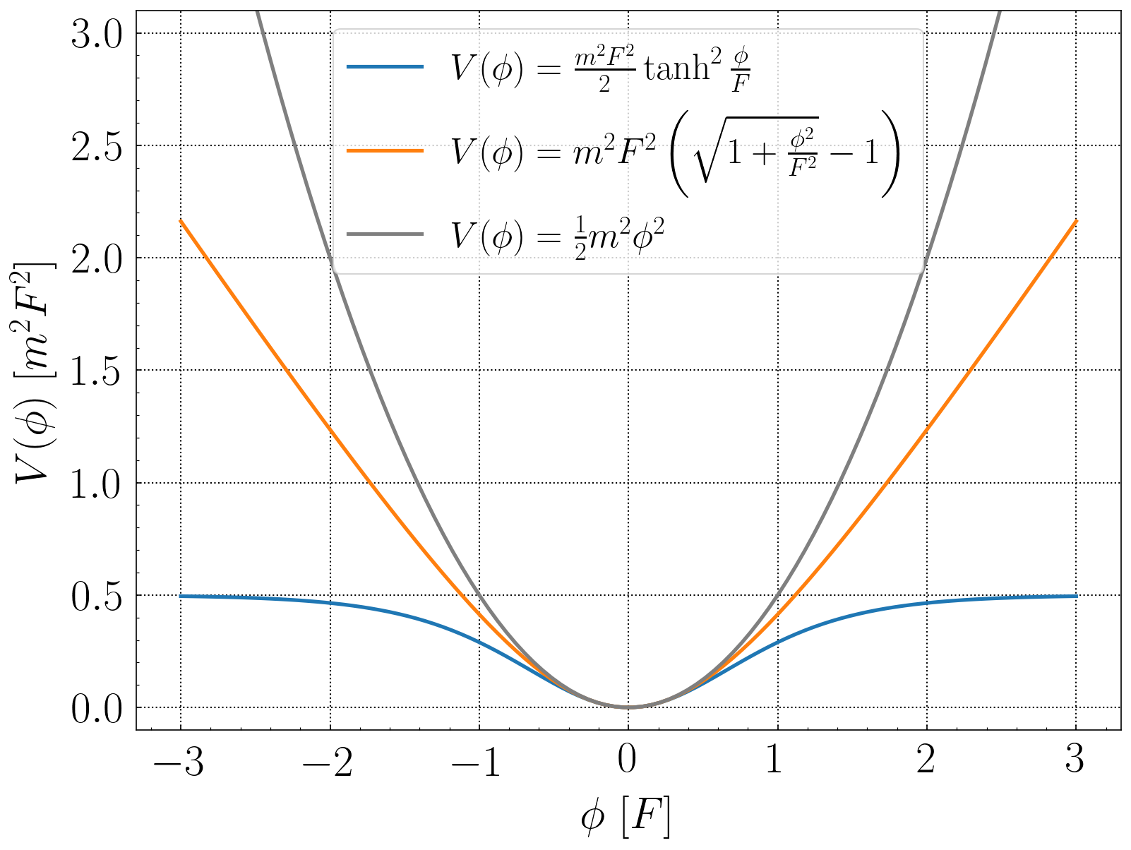
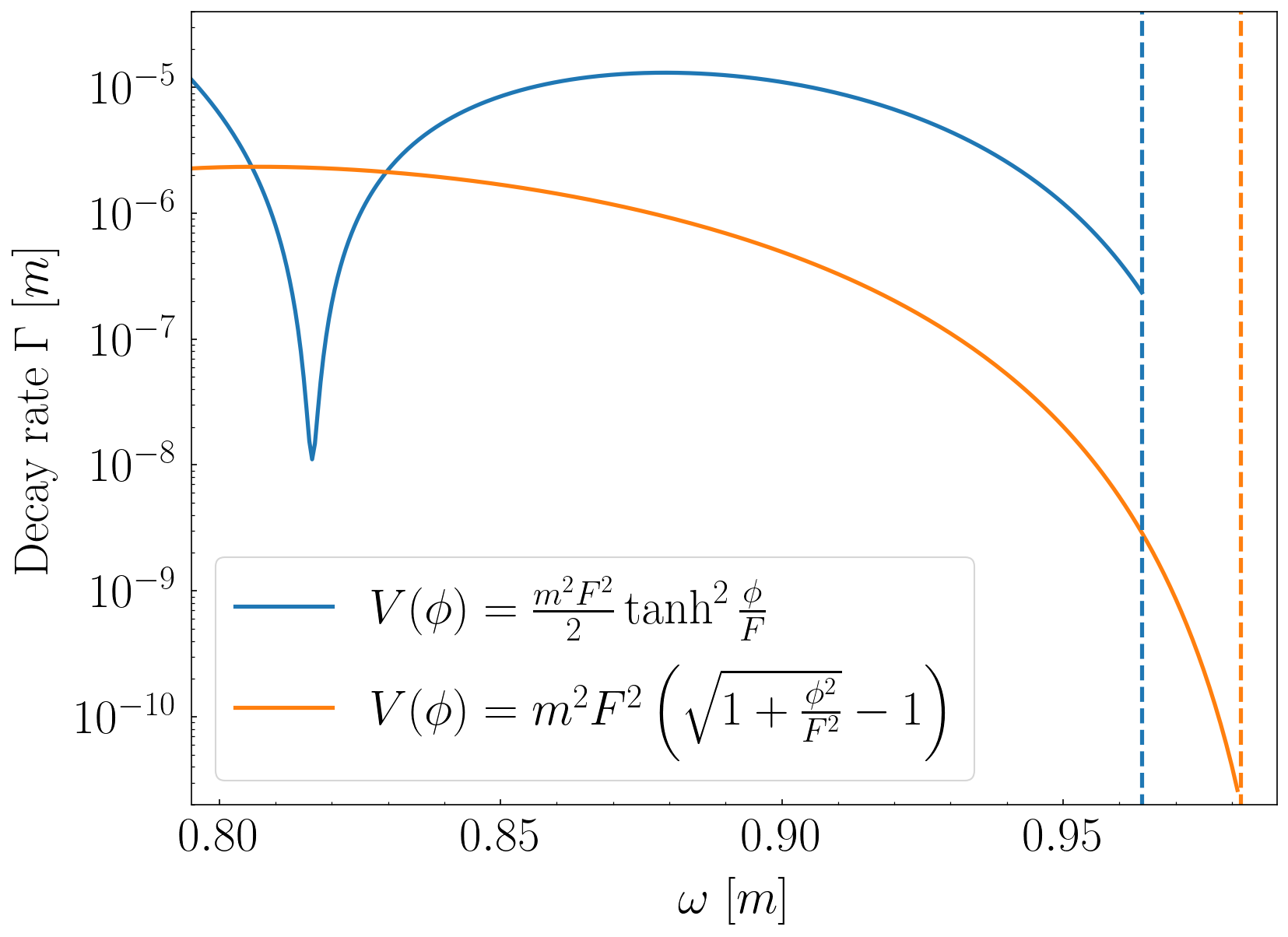
Figure 1: We will consider oscillons in two flattened potentials in this paper (left panel), and semi-analytical calculation of their decay rate is presented for Minkowski spacetime (right panel). The dashed lines indicate the location of $\omega_{\mathrm{crit}}$, at which oscillons finally decay away due to instabilities to small fluctuations.

The gravitational effects on oscillon decay rates are expected to depend on the relative magnitude between gravitational and self- interactions. In 3+1 dimensions, the lifetime of small-amplitude dilute oscillons (whose self-interactions are negligible) was shown to exceed the present age of the universe Grandclement:2011wz ; Eby:2015hyx ; Eby:2020ply . What was not clear to us is whether the existence of gravity stablizes large-amplitude dense ones, whose self-interactions are more or at least equally important. In this paper, we will study two well-motivated examples to explore this impact, the $\alpha$-attractor T-model of inflation Kallosh:2013hoa ; Lozanov:2017hjm and the axion monodromy model Silverstein:2008sg ; Amin:2011hj ; McAllister:2014mpa

$$V(\phi)=\frac{m^{2}F^{2}}{2}\tanh^{2}\frac{\phi}{F}~{},\quad V(\phi)=m^{2}F^{2}\left(\sqrt{1+\frac{\phi^{2}}{F^{2}}}-1\right)~{},$$ (1)

where $F$ is the amplitude scale that indicates a significant deviation from a quadratic minimum, see the left panel of figure 1.

Throughout the paper we will assume classical field theory and spherical symmetry. The first assumption is a standard procedure to deal with compact objects like dense oscillons due to their particularly large occupation number Guth:2014hsa . We also stick to the second one because it simplifies the problem quite a bit and non-spherical components usually decay rapidly with little disturbance on oscillon evolution Seidel:1993zk ; Hindmarsh:2006ur . Even if the early inhomogeneities forming oscilllons possess angular momentum, a non-axisymmetric instability seems to develop and ejects all the angular momentum from the scalar star Sanchis-Gual:2019ljs .

The rest of this paper is organized as follows. In section 2, we briefly review the method developed in Zhang:2020bec to calculate oscillon decay rates and lifetimes in Minkowski spacetime. In section 3, we introduce a Lagrangian mechanism and define the mass and energy of oscillons in curved spacetime. In section 4, we generalize the method to calculate oscillon decay rates and lifetimes in the non-relativistic limit and weak-field limit of gravity. Then we discuss the gravitational effects on oscillon lifetimes in section 5 and make conclusions in section 6. In appendix A and B, we provide analytical expressions for cosine series of the scalar potential and describe numerical algorithms for full GR simulations respectively. We will adopt the natural units $c=\hbar=1$, and frequently use the reduced Planck mass defined by $M_{\mathrm{pl}}\equiv(8\pi G)^{-1/2}\sim 10^{18}\mathrm{GeV}$.

2 Oscillons in Minkowski spacetime

We study oscillon dynamics in Minkowski spacetime in this section. In section 2.1, we briefly review a model-independent calculation of oscillon decay rates and lifetimes following our earlier work Zhang:2020bec . Then in section 2.2, we derive a virial theorem and introduce some small parameters that will allow us to simplify equations when gravitational effects are included.

2.1 Profiles, decay rates and lifetimes

Let us begin with a real-valued scalar field with the Lagrangian given by

$$\mathcal{L}=-\frac{1}{2}g^{\mu\nu}\partial_{\mu}\phi\partial_{\nu}\phi-\frac{1}{2}m^{2}\phi^{2}-V_{\mathrm{nl}}(\phi)~{},$$ (2)

where $g_{\mu\nu}=\mathrm{diag}(-1,1,1,1)$ is the Minkowski metric and $V_{\mathrm{nl}}(\phi)$ is the nonlinear part of the potential $V(\phi)$. The equation of motion is the Klein-Gordon equation

$$\left[-\partial_{t}^{2}+\nabla^{2}-m^{2}\right]\phi-V_{\mathrm{nl}}^{\prime}(\phi)=0~{},$$ (3)

where $\nabla^{2}\equiv\partial_{r}^{2}+(2/r)\partial_{r}$. For simplicity we will only consider symmetric potentials, but the method developed in this paper should also be applicable to asymmetric ones. As suggested in Seidel:1991zh , we approximate oscillons by a cosine series

$$\phi(t,r)=\phi_{\mathrm{osc}}(t,r)+\xi(t,r)=\phi_{1}(r)\cos(\omega t)+\sum_{j=3}^{\infty}\xi_{j}(r)\cos(j\omega t)~{},$$ (4)

where $j$ is odd, $\phi_{\mathrm{osc}}$ is a single-frequency profile and $\xi(t,r)$ includes all the radiating modes. Typically $|\xi|\ll|\phi_{\mathrm{osc}}|$ inside oscillons. As a result, the potential and its derivatives can also be written in terms of the Fourier cosine series

$$U \equiv V_{\mathrm{nl}}(\phi_{\mathrm{osc}})=\frac{1}{2}U_{0}(r)+\sum_{j=2}^{\infty}U_{j}(r)\cos(j\omega t)\quad\text{and}\quad U_{j}=\frac{\omega}{\pi}\int_{-\frac{\pi}{\omega}}^{\frac{\pi}{\omega}}V_{\mathrm{nl}}(\phi_{\mathrm{osc}})\cos(j\omega t)dt~{},$$ (5)

$$M \equiv V_{\mathrm{nl}}^{\prime\prime}(\phi_{\mathrm{osc}})=\frac{1}{2}M_{0}(r)+\sum_{j=2}^{\infty}M_{j}(r)\cos(j\omega t)\quad\text{and}\quad M_{j}=\frac{\omega}{\pi}\int_{\frac{\pi}{\omega}}^{\frac{\pi}{\omega}}V_{\mathrm{nl}}^{\prime\prime}(\phi_{\mathrm{osc}})\cos(j\omega t)dt~{}.$$ (6)

where $j$ is even, and

$$J\equiv V_{\mathrm{nl}}^{\prime}(\phi_{\mathrm{osc}})=\sum_{j=1}^{\infty}J_{j}(r)\cos(j\omega t) \quad\text{and}\quad J_{j}=\frac{\omega}{\pi}\int_{-\frac{\pi}{\omega}}^{\frac{\pi}{\omega}}V_{\mathrm{nl}}^{\prime}(\phi_{\mathrm{osc}})\cos(j\omega t)dt~{},$$ (7)

where $j$ is odd. The $U_{j}$ is a functional of $\phi_{1}$ hence a function of $r$, namely $U_{j}(\phi_{1})\equiv U_{j}(r)$. We will mix the notation $U_{j}(\phi_{1})$ and $U_{j}(r)$, and similarly for $J_{j}$ and $M_{j}$. For polynomial potentials, it is possible to find analytical expressions for $U_{j},M_{j}$ and $J_{j}$. These are provided in appendix A.

Plugging the single-frequency profile $\phi_{\mathrm{osc}}$ into the Kelin-Gordon equation and collecting the coefficient of $\cos(\omega t)$, we obtain the radial profile equation

$$(\nabla^{2}+\kappa_{1}^{2})\phi_{1}(r)=J_{1}(r)~{},$$ (8)

where $\kappa_{j}^{2}\equiv(j\omega)^{2}-m^{2}$ is the square of the momentum for a particular mode and we have used $J_{1}(\phi_{1})=U_{0}^{\prime}(\phi_{1})$. Oscillon profiles can be found by using the numerical shooting method and by demanding a localized, smooth and no-node solution for each $\omega$. Without loss of generality, we assume that the minimum of $V(\phi)$ is located at $\phi=0$ thus the boundary condition is $\phi_{1}(\infty)=0$. Once the profile is found, the energy of oscillons can be obtained by time averaging the energy density over a period, and is given by

$$E_{\mathrm{osc}}=\int_{0}^{\infty}\left[\frac{1}{4}\left(\partial_{r}\phi_{1}\right)^{2}+\frac{1}{4}(\omega^{2}+m^{2})\phi_{1}^{2}+\frac{1}{2}U_{0}\right]4\pi r^{2}dr~{}.$$ (9)

For these single frequency objects, we can define the particle number Mukaida:2016hwd

$$N_{\mathrm{osc}}=\frac{\omega}{2}\int_{0}^{\infty}\phi_{1}^{2}~{}4\pi r^{2}dr~{}.$$ (10)

The stability condition of oscillons against small perturbations is given by Friedberg:1976me

$$\frac{dN_{\mathrm{osc}}}{d\omega}<0\quad\text{or}\quad\frac{dE_{\mathrm{osc}}}{d\omega}<0~{},$$ (11)

and the critical frequency $\omega_{\mathrm{crit}}$ can be obtained by setting $dE_{\mathrm{osc}}/d\omega=0$.

Radial equations for radiating modes can be obtained by plugging the full expansion (4) into the Klein-Gordon equation and collecting the coefficient of $\cos(j\omega t)$, i.e.

$$\left[\nabla^{2}+\kappa_{j}^{2}\right]\xi_{j}(r)=S_{j}(r)\equiv J_{j}+\frac{1}{2}\sum_{k=3}^{\infty}\xi_{k}\left(M_{|k+j|}+M_{|k-j|}\right)~{},$$ (12)

where $j$ and $k$ are both odd, $S_{j}$ is the effective source and $M_{j}$ is the effective mass. For $\kappa_{j}^{2}>0$, the central amplitude of a radiating mode is

$$\xi_{j}(0)=-\int_{0}^{\infty}dr^{\prime}~{}S_{j}(r^{\prime})~{}r^{\prime}\cos(\kappa_{j}r^{\prime})~{}.$$ (13)

This is not in closed form, and we can find the solution of $\xi_{j}(r)$ by using the iterative method developed in Zhang:2020bec . The energy loss rate of oscillons is determined by radiation at large radius

$$\frac{dE_{\mathrm{osc}}}{dt}=-4\pi r^{2}\tensor{T}{{}^{1}_{0}}|_{r\rightarrow\infty}=\left.-4\pi r^{2}\partial_{t}\xi\partial_{r}\xi\right|_{r\rightarrow\infty}~{}$$

where $\tensor{T}{{}^{\mu}_{\nu}}=\partial^{\mu}\phi\partial_{\nu}\phi+\delta^{\mu}_{\nu}\mathcal{L}$ is the energy-momentum tensor and the radiation is given by

$$\left.\xi(t,r)\right|_{r\rightarrow\infty}=-\frac{1}{4\pi r}\sum_{j=3}^{\infty}\tilde{S}_{j}(\kappa_{j})\cos(\kappa_{j}r-j\omega t)~{}.$$ (14)

Here $\tilde{S}_{j}(p)$ is the Fourier transform of the effective source

$$\tilde{S}_{j}(p)=\int_{0}^{\infty}dr~{}4\pi r^{2}\operatorname{sinc}(pr)S(r)~{}.$$ (15)

The (absolute value of) decay rate is defined

$$\Gamma\equiv\left|\langle\dot{E}_{\mathrm{osc}}/E_{\mathrm{osc}}\rangle_{T}\right|=\frac{1}{8\pi E_{\mathrm{osc}}}\sum_{j=3}^{\infty}\left[\tilde{S}_{j}(\kappa_{j})\right]^{2}j\omega~{}\kappa_{j}\equiv\sum_{j=3}^{\infty}\Gamma_{j}~{},$$ (16)

where $\Gamma_{j}$ is the contribution due to $S_{j}$. Typically the radiating mode safisfies $|\xi_{j}|\gg|\xi_{j+2}|$, which means only finite terms are needed in the radial equation (12). However, the leading channel of decay rates $\Gamma_{3}$ might vanish for some $\omega$, causing a dip structure seen in figure 1.

If we start with an oscillon with $\omega<\omega_{\rm dip}$, the frequency of the oscillons evolves to larger values by slowly emitting scalar radiation (and the profile changes correspondingly). Since the leading decay channel $\Gamma_{3}$ is vanishing in the dip, the oscillon configuration with $\omega\approx\omega_{\rm dip}$ is expected to have a long lifetime. When considering the total lifetime of oscillons that start out at $\omega<\omega_{\rm dip}$, the oscillon will spend most of its lifetime in such a dip. Generally speaking, we will use $\Gamma_{3}+\Gamma_{5}$ to estimate the lifetime of oscillons, which is just the area enclosed by the evolution curve in $dt/dE_{\mathrm{osc}}$ versus $E_{\mathrm{osc}}$ plot, where $dt/dE_{\mathrm{osc}}=1/(\Gamma E_{\mathrm{osc}})$. For future reference, if we keep only $\xi_{3}$ and $\xi_{5}$, the effective source becomes

$$S_{3} =J_{3}+\frac{1}{2}\xi_{3}(M_{0}+M_{6})+\frac{1}{2}\xi_{5}(M_{2}+M_{8})~{},$$ (17)

$$S_{5} =J_{5}+\frac{1}{2}\xi_{3}(M_{2}+M_{8})+\frac{1}{2}\xi_{5}(M_{0}+M_{10})~{}.$$ (18)

The generalization to including more $\xi_{j}$ terms is straightforward. Note that the effective source $S_{j}$ receives a contribution from the oscillon background $J_{j}$ as well as corrections due to radiation $\xi_{j}$.

2.2 A virial theorem and small parameters

Assume that oscillons are single-frequency objects like Q-balls and Boson stars Lee:1991ax , then one way to derive a virial theorem is to use the variational principle. The Legendre transformation

$$F_{\mathrm{osc}}=\omega N_{\mathrm{osc}}-E_{\mathrm{osc}}$$ (19)

defines a functional of $\phi_{1}$ and a function of $\omega$ (one may recognize that $F_{\mathrm{osc}}$ is just the Lagrangian). The variation of $F_{\mathrm{osc}}$ in terms of $\phi_{1}$ by keeping $\omega$ fixed gives the profile equation of oscillons (8). A virial theorem can be obtained by considering the variation $\phi_{1}(r)\rightarrow\phi_{1}(\lambda r)$ for an oscillons solution. By setting $\left(\partial F_{\mathrm{osc}}/\partial\lambda\right)_{\omega}=0$ at $\lambda=1$, we find

$$E_{\mathrm{S}}/3+E_{\mathrm{V}}=E_{\mathrm{K}}~{},$$ (20)

where the surface energy, potential energy and kinetic energy are defined

$$E_{\mathrm{S}}=\int\frac{1}{4}(\partial_{r}\phi_{1})^{2}d^{3}r~{},\quad E_{\mathrm{V}}=\int\left(\frac{1}{4}m^{2}\phi_{1}^{2}+\frac{1}{2}U_{0}\right)d^{3}r~{},\quad E_{\mathrm{K}}=\int\frac{1}{4}\omega^{2}\phi_{1}^{2}~{}d^{3}r~{}.$$ (21)

For oscillons with $\omega\lesssim m$, we can identify three small parameters immediately

$$\epsilon_{r}\equiv 1-\omega^{2}/m^{2}~{},\quad\epsilon_{V}\sim\frac{U_{0}}{m^{2}\phi_{1}^{2}/2}~{},\quad\epsilon_{\xi}\sim\frac{\xi_{j}}{\phi_{1}}~{}.$$ (22)

The parameter $\epsilon_{r}$ is a measure of how relativistic the particles inside the oscillon are. Equation (8) implies that at large radius $\phi_{1}(r)\propto r^{-1}\exp\left[-(m^{2}-\omega^{2})^{1/2}r\right]$, hence a typical spatial derivative brings a factor $\sqrt{\epsilon_{r}}m$, that is, $\partial_{r}\phi_{1}\sim-\sqrt{\epsilon_{r}}m\phi_{1}$, and

$$\nabla^{2}\phi_{1}\ll\omega^{2}\phi_{1}~{}.$$ (23)

This means that the particles that make up the oscillon are non-relativistic. And from equations (12) and (20), we see $\epsilon_{\xi}\sim-\epsilon_{V}$ and $\epsilon_{V}\sim-\epsilon_{r}$.

For oscillons with $\omega\ll m$, we may not regard surface energy as a small quantity anymore. Take the tanh potential in (1) for example and assume a Gaussian profile

$$\phi_{1}(r)=C~{}e^{-r^{2}/R^{2}}~{},$$ (24)

where $C\gg F$. Then each energy component becomes

$$E_{\mathrm{S}}\sim C^{2}R~{},\quad E_{\mathrm{K}}\sim C^{2}R^{3}\omega^{2}\sim\frac{N_{\mathrm{osc}}^{2}}{C^{2}R^{3}}~{},\quad E_{\mathrm{V}}\sim R_{\mathrm{V}}^{3}m^{2}F^{2}~{},$$ (25)

where we have taken advantage of the flatness of the potential at large $\phi$ and $R_{\mathrm{V}}$ is the length scale satisfying $\phi_{1}(R_{\mathrm{V}})\sim\mathcal{O}(1)$, i.e.

$$R_{\mathrm{V}}\sim R\log^{1/2}\left(\frac{C}{F}\right)\sim R~{}.$$ (26)

By setting $\partial E_{\mathrm{osc}}/\partial R=\partial E_{\mathrm{osc}}/\partial C=0$ and keeping $N_{\mathrm{osc}}$ fixed, we obtain

$$R\sim\omega^{-1}~{},\quad C\sim\omega^{-1}~{}.$$ (27)

We see that three components of energy now are all comparable, and thus oscillon particles are relativistic. This phenomenon has been witnessed numerically in the context of dense axion stars Visinelli:2017ooc ; Eby:2019ntd .

3 Full GR formalism

So far our analysis does not include gravity. In this section, the scalar field is assumed to be minimally coupled to gravity. We introduce a Lagrangian mechanism that can convert the Hilbert action into one that contains only the first derivative of the metric in section 3.1, then we use it to generalize the definition of energy and mass into curved spacetime in section 3.2.

3.1 A Lagrangian mechanism

The simplest choice of metric to describe oscillons is the spherical coordinates

$$ds^{2}=-e^{2\Phi(t,r)}\mathrm{d}t^{2}+e^{-2\Psi(t,r)}\mathrm{d}r^{2}+r^{2}(\mathrm{d}\theta^{2}+\sin^{2}\theta~{}\mathrm{d}\varphi^{2})~{},$$ (28)

where $\theta,\varphi$ are the polar and azimuthal angles, $r$ is $(2\pi)^{-1}$ times the circumference of a two-sphere. The action of our theory is composed of the action of gravity and matter $S=S_{\mathrm{G}}+S_{\mathrm{M}}$, specifically

$$S_{\mathrm{G}} =\frac{1}{16\pi G}\left(\int_{\Omega}R\sqrt{-g}~{}d^{4}x+\int_{\partial\Omega}K\sqrt{|h|}~{}d^{3}x\right)~{},$$ (29)

$$S_{\mathrm{M}} =\int\left[-\frac{1}{2}g^{\mu\nu}\phi_{,\mu}\phi_{,\nu}-V(\phi)\right]\sqrt{-g}~{}d^{4}x~{},$$ (30)

where $\phi_{,\mu}\equiv\partial_{\mu}\phi$ is defined for notation convenience, $R$ is the Ricci scalar and $g$ is the determinant of $g_{\mu\nu}$, i.e.

$$R= 2r^{-2}-2e^{-2\Phi}\left[\Psi_{,00}-\Psi_{,0}(\Phi+\Psi)_{,0}\right]$$ (31)

$$-2e^{2\Psi}\left[r^{-2}+2r^{-1}(\Phi+\Psi)_{,1}+\Phi_{,1}(\Phi+\Psi)_{,1}+\Phi_{,11}\right]~{},$$ (32)

$$\sqrt{-g}~{}d^{4}x= e^{\Phi-\Psi}r^{2}\sin\theta~{}dt~{}dr~{}d\theta~{}d\varphi~{}.$$ (33)

Apart from the standard Hilbert action, $K$ is a surface term and $h$ is the induced metric on the boundary $\partial\Omega$ Gibbons:1976ue that can be appropriately chosen Lee:1988av , i.e.

$$K =2e^{\Psi}\Phi_{,1}+4r^{-1}(e^{\Psi}-1)~{},$$ (34)

$$\sqrt{|h|}~{}d^{3}x =e^{\Phi}r^{2}\sin\theta~{}dt~{}d\theta~{}d\varphi~{},$$ (35)

for the three dimensional surface at $r=r_{0}$ and

$$K =2e^{-\Phi}\Psi_{,0}~{},$$ (36)

$$\sqrt{|h|}~{}d^{3}x =e^{-\Psi}r^{2}\sin\theta~{}dr~{}d\theta~{}d\varphi~{},$$ (37)

for that which is bounded by $t=\pm T$. The inclusion of surface terms will not change the Einstein equations, but can convert the Hilbert action into one that contains only the first derivative of the metric so that the usual Lagrangian mechanics can be applied. After setting $r_{0}$ and $T\rightarrow\infty$, the Lagrangian, i.e. $S=\int L~{}dt$, becomes

$$L_{\mathrm{G}} =(2G)^{-1}\int_{0}^{\infty}\left[e^{\Phi-\Psi}+e^{\Phi+\Psi}(1+2r\Phi_{,1})-2e^{\Phi}(1+r\Phi_{,1})\right]dr~{},$$ (38)

$$L_{\mathrm{M}} =\int_{0}^{\infty}(X-Y-V)~{}e^{\Phi-\Psi}4\pi r^{2}dr~{},$$ (39)

where we have defined

$$X\equiv\frac{1}{2}e^{-2\Phi}\phi_{,0}^{2}~{},\quad Y\equiv\frac{1}{2}e^{2\Psi}\phi_{,1}^{2}~{}.$$ (40)

The gravity and matter are related by the Einstein equation

$$\tensor{G}{{}_{\mu}{}_{\nu}}=\tensor{R}{{}_{\mu}{}_{\nu}}-\frac{1}{2}g_{\mu\nu}R=8\pi G~{}\tensor{T}{{}_{\mu}{}_{\nu}}~{},$$ (41)

where $R_{\mu\nu}$ is the Ricci tensor and the energy-momentum tensor $\tensor T{{}^{\mu}_{\nu}}$ is given by

$$T_{\mu\nu}=-2\frac{1}{\sqrt{-g}}\frac{\delta S_{\mathrm{M}}}{\delta g^{\mu\nu}}=\phi_{,\mu}\phi_{,\nu}-\frac{1}{2}g_{\mu\nu}g^{\rho\sigma}\phi_{,\rho}\phi_{,\sigma}-g_{\mu\nu}V(\phi)~{}.$$ (42)

More specifically

$$\tensor{G}{{}^{0}_{0}} =r^{-2}\left(e^{2\Psi}-1+2r\Psi_{,1}e^{2\Psi}\right)=-8\pi G(X+Y+V)~{},$$ (43)

$$\tensor{G}{{}^{1}_{0}} =-2r^{-1}\Psi_{,0}e^{2\Psi}=8\pi G~{}e^{2\Psi}\phi_{,0}\phi_{,1}~{},$$ (44)

$$\tensor{G}{{}^{1}_{1}} =r^{-2}\left(e^{2\Psi}-1+2r\Phi_{,1}e^{2\Psi}\right)=8\pi G(X+Y-V)~{},$$ (45)

$$\tensor{G}{{}^{2}_{2}} =e^{-2\Phi}\left[\Psi_{,00}-\Psi_{,0}(\Phi+\Psi)_{,0}\right]+e^{2\Psi}\left[\Phi_{,11}+(\Phi_{,1}+r^{-1})(\Phi+\Psi)_{,1}\right]=8\pi G(X-Y-V)~{},$$ (46)

where $\tensor{G}{{}^{3}_{3}}=\tensor{G}{{}^{2}_{2}}$ and all other components vanish. The $\tensor{G}{{}^{0}_{0}}$ and $\tensor{G}{{}^{1}_{1}}$ equations can be alternatively obtained by varying the Lagrangian with respect to $\Phi$ and $\Psi$. The others can be derived using the contracted Bianchi identity $\tensor{G}{{}^{\mu}_{\nu;\mu}}=0$, i.e. $\nu=0$ gives (44), $\nu=2$ gives $\tensor{G}{{}^{2}_{2}}=\tensor{G}{{}^{3}_{3}}$ and $\nu=1$ gives (46). Some combanitions will be useful, for example, equations (43) and (45) give

$$r^{-1}e^{2\Psi}(\Phi-\Psi)_{,1}=8\pi G(X+Y)~{},$$ (47)

and equations (46) and (47) give

$$e^{-2\Phi}\left[\Psi_{,00}-\Psi_{,0}(\Phi+\Psi)_{,0}\right]+e^{2\Psi}\left[\nabla^{2}\Phi+\Phi_{,1}(\Phi+\Psi)_{,1}\right]=8\pi G(2X-V)~{},$$ (48)

where $\nabla^{2}\equiv\partial_{r}^{2}+(2/r)\partial_{r}$. The equation of motion of $\phi$ is

$$e^{-2\Phi}\left[-\phi_{,00}+(\Phi+\Psi)_{,0}\phi_{,0}\right]+e^{2\Psi}\left[\nabla^{2}\phi+(\Phi+\Psi)_{,1}\phi_{,1}\right]-V^{\prime}(\phi)=0~{},$$ (49)

which is obtained by varying the Lagrangian with respect to $\phi$.

3.2 Mass and energy

Following Lee:1988av , we distinguish between the mass and energy of oscillons. At large radius the mass density vanishes exponentially, hence $\Phi$ and $\Psi$ scale as $r^{-1}$. The mass then must satisfy

$$M_{\mathrm{osc}}=-G^{-1}\lim\limits_{r\rightarrow\infty}r\Psi=-G^{-1}\lim\limits_{r\rightarrow\infty}r\Phi~{},$$ (50)

to be consistent with the static Schwarzschild solution. There are other ways to express the same mass. For example, the LHS of 00 component of Einstein equation can be rewritten into $r^{-2}[r\left(e^{2\Psi}-1\right)]_{,1}$ hence the mass is also given by

$$M_{\mathrm{osc}}=\int_{0}^{\infty}(X+Y+V)~{}4\pi r^{2}dr=-\int_{0}^{\infty}\tensor{T}{{}^{0}_{0}}~{}4\pi r^{2}dr~{},$$ (51)

which is in agreement with the Schwarzschild mass (50).

A more enlightening way to describe the mass is to use the Hamiltonian formalism. The Lagrangian of matter (39) indicates that the energy of the oscillon is

$$E_{\mathrm{osc}}=\int_{0}^{\infty}(X+Y+V)~{}e^{\Phi-\Psi}4\pi r^{2}dr=-\int\tensor{T}{{}^{0}_{0}}\sqrt{-g}~{}d^{3}x~{}.$$ (52)

There is no kinetic term in the Lagrangian of gravity (38) thus the energy of gravity is $E_{\mathrm{G}}=-L_{\mathrm{G}}$. Then we define the mass of oscillons

$$M_{\mathrm{osc}}\equiv E_{\mathrm{osc}}+E_{G}~{}.$$ (53)

Combining the energy expression and the 00 component of Einstein equations, we find

$$[r(e^{\Phi}-e^{\Phi+\Psi})]_{,1}=G(E_{\mathrm{M}}+E_{\mathrm{G}})_{,1}~{},$$ (54)

in agreement with the Schwarzschild mass (50) and the ADM mass Arnowitt:1962hi . After understanding what we mean by energy, the decay rate of oscillons can be studied numerically in appendix B and analytically in the next section.

4 Oscillons with linearized gravity

The typical central amplitude, radius and mass of dense oscillons in the non-relativistic limit are

$$\phi_{1}(0)\sim F~{},\quad R_{\mathrm{osc}}\sim 5m^{-1}~{},\quad M_{\mathrm{osc}}\sim 100F^{2}/m~{}.$$ (55)

Nonlinear effects of gravitational interactions are not important if the size of oscillons is much smaller than their Schwarzschild radius

$$R_{\mathrm{osc}}\ll GM_{\mathrm{osc}}\Rightarrow\epsilon_{\phi}\sim\phi_{1}/M_{\mathrm{pl}}\ll 1~{},$$ (56)

which is satisfied by a number of cosmological models. In this section, therefore, we study the decay rate and lifetime of oscillons in the non-relativistic limit and weak-field limit of gravity, specifically those with $\epsilon_{r}\lesssim 0.1$ and $\epsilon_{\phi}\lesssim 0.1$. The basic idea is similar to what we have done in section 2.

4.1 Profiles

In the weak-field approximation, the spherical metric (28) reduces to

$$ds^{2}=-(1+2\Phi)\mathrm{d}t^{2}+(1-2\Psi)\mathrm{d}r^{2}+r^{2}(\mathrm{d}\theta^{2}+\sin^{2}\theta~{}\mathrm{d}\varphi^{2})~{}.$$ (57)

So far we have encountered five sets of small dimensionless parameters, recall equations (22) and (56), i.e. the spatial derivative parameter $\epsilon_{r}$, the nonlinear potential parameter $\epsilon_{V}$, the radiation parameter $\epsilon_{\xi}$, the amplitude parameter $\epsilon_{\phi}$ and the gravitational potentials $\Phi$ and $\Psi$ (denoted by $\epsilon_{g}$). To be consistent, we will keep all small quantities to 1st order, and to 2nd order if spatial derivatives of small parameters are involved. Then the equation of motion of $\phi$ (49) becomes

$$-(1-2\Phi)\phi_{,00}+(\Phi+\Psi)_{,0}\phi_{,0}+\nabla^{2}\phi-V^{\prime}(\phi)=\mathcal{O}(\epsilon^{2}m^{2}\phi)~{}.$$ (58)

To be consistent with the field expansion (4), we expand the gravitational potentials in terms of a Fourier cosine series

$$\Phi=\frac{1}{2}\Phi_{0}+\sum_{j=2}^{\infty}\Phi_{j}\cos(j\omega t)~{},\quad\Psi=\frac{1}{2}\Psi_{0}+\sum_{j=2}^{\infty}\Psi_{j}\cos(j\omega t)~{},$$ (59)

where $j$ is even. We can solve these radial modes by plugging the expansion into the Einstein equations and collecting the coefficient for each Fourier mode. Then equations (44) and (45) give

$$\Psi_{0}=-r\Phi_{0,1}+\mathcal{O}(\epsilon^{2})~{},\quad\Psi_{2}=\mathcal{O}(\epsilon^{2})~{},\quad\Psi_{j\geq 4}=\mathcal{O}(\epsilon^{3})~{},$$ (60)

and equations (47) and (48) give

$$\nabla^{2}\Phi_{0}=4\pi G~{}m^{2}\phi_{1}^{2}+\mathcal{O}(\epsilon^{3}m^{2})~{},\quad\Phi_{2,1}/r=-2\pi G~{}m^{2}\phi_{1}^{2}+\mathcal{O}(\epsilon^{3}m^{2})~{},\quad\Phi_{j\geq 4}=\mathcal{O}(\epsilon^{2})~{}.$$ (61)

Therefore, $-\Phi_{0}\sim-\Psi_{0}\sim\Phi_{2}\sim\epsilon_{g}\sim\epsilon_{\phi}^{2}/\epsilon_{r}$. Somewhat surprisingly, we find $\Phi_{2}$ and $\Psi_{2}$ are not the same order of magnitude, in constrast with the common results of the Newtonian gauge. We will ignore $\Phi_{j\geq 4}$ and $\Psi_{j\geq 2}$ in future calculations.

In order to find the profile of oscillons, we plug the field expansion (4) and (59) into equation (58) and collect the coefficient of $\cos(\omega t)$ to get

$$[\nabla^{2}+\omega^{2}(1-\Phi_{0})-m^{2}]\phi_{1}=J_{1}+\mathcal{O}(\epsilon^{2}m^{2}\phi_{1})~{}.$$ (62)

Here $\omega(1-\Phi_{0})^{1/2}$ can be regarded as an effective frequency and is larger than $\omega$. This equation can be solved by numerical shooting method. The time-averaged formula for the oscillon energy (52) is

$$E_{\mathrm{osc}}=\int_{0}^{\infty}\left[\frac{1}{4}(\partial_{r}\phi_{1})^{2}+\frac{1}{4}(\omega^{2}+m^{2})\left(1-\frac{1}{2}\Psi_{0}+\frac{1}{2}\Phi_{2}\right)\phi_{1}^{2}+\frac{1}{2}U_{0}\right]4\pi r^{2}dr+\mathcal{O}\left(\frac{\epsilon^{1/2}\phi_{1}^{2}}{m}\right)~{}.$$ (63)

As long as the oscillating part of the gravitational potentials is not too important, namely $\epsilon_{g}\lesssim 0.1$, oscillons share great similarities with mini-boson stars Friedberg:1986tp , and we assume the stability condition is still valid Lee:1988av

$$\frac{dE_{\mathrm{osc}}}{d\omega}<0~{}.$$ (64)

This is confirmed by comparing analytical predictions of $\omega_{\mathrm{crit}}$ with numerical results in the left panel of figure 4.

4.2 Decay rates

Plugging the field expansion (4) and (59) into equation (58) and collecting the coefficient of $\cos(j\omega t)$, we obtain the radial equation of radiating modes

$$\left[\nabla^{2}+\kappa_{j}^{2}\right]\xi_{j}(r)=S_{j}(r)+\mathcal{O}(\epsilon^{3}m^{2}\phi_{1})~{},$$ (65)

where $j\geq 3$ and $j$ is odd, and $S_{j}$ is the effective source. We can keep finite terms of $\xi_{j}$ as we did in Minkowski spacetime. In particular, if we keep only $\xi_{3}$ and $\xi_{5}$, the effective source becomes

$$S_{3} =J_{3}+\frac{1}{2}\xi_{3}(M_{0}+M_{6})+\frac{1}{2}\xi_{5}(M_{2}+M_{8})+2\omega^{2}\phi_{1}\Phi_{2}+9\omega^{2}\xi_{3}\Phi_{0}+20\omega^{2}\xi_{5}\Phi_{2}~{},$$ (66)

$$S_{5} =J_{5}+\frac{1}{2}\xi_{3}(M_{2}+M_{8})+\frac{1}{2}\xi_{5}(M_{0}+M_{10})+12\omega^{2}\xi_{3}\Phi_{2}+25\omega^{2}\xi_{5}\Phi_{0}~{},$$ (67)

where we have kept higher-order perturbations $\xi_{5}\Phi_{j}$ because of their large coefficients. Comparing (66) with the corresponding expression in Minkowski spacetime (17), new corrections are introduced due to the coupling of gravity to oscillons and their radiation. The radiation equation can be solved by the iterative method Zhang:2020bec .

The conservation law of the energy-momentum tensor is

$$\tensor{T}{{}^{\mu}_{\nu;\mu}}=0\Rightarrow(\tensor{T}{{}^{\mu}_{\nu}}\sqrt{-g})_{,\mu}=0~{},$$ (68)

which implies

$$\frac{dE_{\mathrm{osc}}}{dt}=\int(\tensor{T}{{}^{i}_{0}}\sqrt{-g})_{,i}~{}d^{3}x=\left.-4\pi r^{2}\tensor{T}{{}^{i}_{0}}(1+\Phi-\Psi)\right|_{r\rightarrow\infty}=\left.-4\pi r^{2}\xi_{,0}\xi_{,1}\right|_{r\rightarrow\infty}~{},$$ (69)

where we have used Gauss’s divergence theorem to obtain the second equal sign. The $\xi$ at infinity is calculated in (14), then the decay rate expression is just the same as the one in Minkowski spacetime (16).

5 Examples

In this section, we will explore gravitational effects on oscillon lifetimes by studying two examples, recall figure 1 and equation (1), and comparing numerical results from full GR simulations with our analytical predictions. The numerical algorithm is described in appendix B.

5.1 The $\alpha$-attractor T-model of inflation

The longevity of oscillons in this model (whose lifetime $\sim 10^{6}\,m^{-1}$ in Minkowski spacetime) is characterized by a dip structure in decay rates, see figure 1. In the dip, the leading channel of decay rates $\Gamma_{3}$ vanishes and the scalar radiation is dominated by the subleading channel $\Gamma_{5}$. Now we argue that the existence of gravity reduces the lifetime of oscillons.

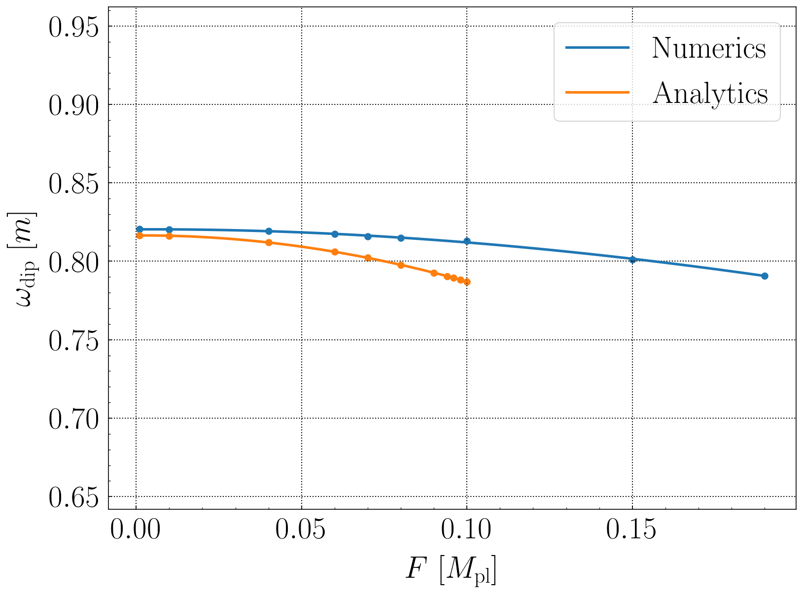
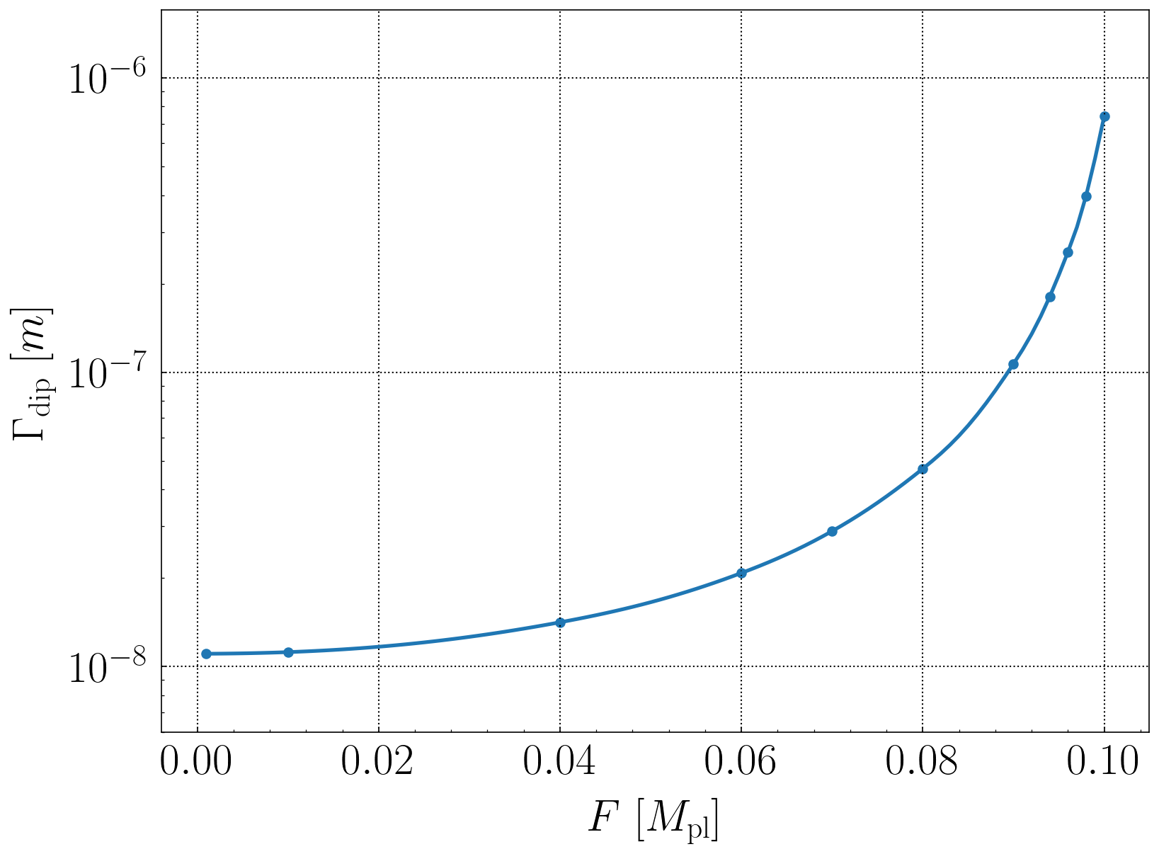
Figure 2: Evidence that the existence of gravity reduces the lifetime of oscillons in the $\alpha$-attractor T-model. In the left panel, we show the dependence of dip locations on values of the characteristic mass scale $F$. The smaller value of $\omega_{\mathrm{dip}}$ is an indication of a shorter lifetime of oscillons, since the amplitude of radiating modes (in unit of $F$) is inversely related to frequencies and thus larger decay rates are expected. In the right panel, we confirm this expectation by explicitly calculating the decay rate at $\omega_{\mathrm{dip}}$.

We first study how the location of the dip is affected both analytically and numerically in figure 2 (left panel). The value of $\omega_{\mathrm{dip}}$ is significantly reduced when the mass scale $F$ approaches the reduced Planck mass. A smaller value of $\omega_{\mathrm{dip}}$ is an indication of shorter lifetimes, since the amplitude of radiating modes (in unit of $F$) is inversely related to frequencies and thus larger decay rates are expected. The comparison between analytics and numerics also provides a chance to test our formalism, which correctly captures the gravitational effect on $\omega_{\mathrm{dip}}$ as long as the assumptions of weak-field gravity and non-relativistic limit remain valid.

To exclude the possibility that the subleading channel of decay rates also vanishes, we explicitly calculate $\Gamma_{5}$ around $\omega_{\mathrm{dip}}$ as shown in figure 2 (right panel). As a determinant factor, the increasing of $\Gamma_{\mathrm{dip}}\approx\Gamma_{5}$ is a clear evidence that the existence of gravity reduces the lifetime of oscillons, which has also been confirmed numerically. For convenience, we present a direct visualization of these two factors in figure 3.

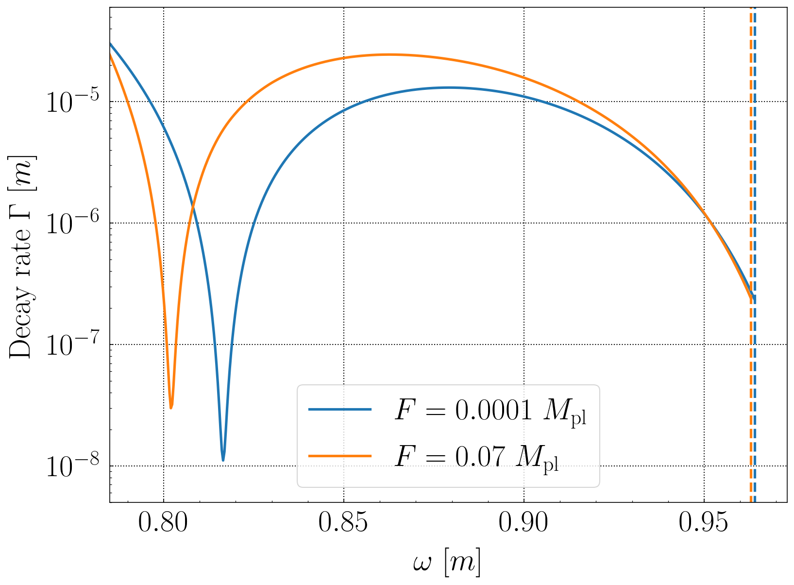
Figure 3: A comparison of decay rates for two different values of $F$ in the $\alpha$-attractor T-model.

5.2 The axion monodromy model

In constrast with the $\alpha$-attractor T-model, the subleading channel of decay rates $\Gamma_{5}$ is never comparable with the leading channel $\Gamma_{3}$ in the axion monodromy model. The longevity of oscillons in this case (whose lifetime $\sim 10^{8}\,m^{-1}$ in Minkowski spacetime) is due to the dramatic suppresion of $\Gamma_{3}$ just before their final collapse at $\omega_{\mathrm{crit}}$. Consequently, there are two factors that determine the lifetime of oscillons, the value of $\omega_{\mathrm{crit}}$ and the decay rate around $\omega_{\mathrm{crit}}$.

In figure 4 (left panel), we show that the values of $\omega_{\mathrm{crit}}$ are inversely related to $F$. This seems an indication of shorter lifetimes for stronger gravitational effects because oscillons now spend less time around $\omega_{\mathrm{crit}}$. A good match between analytics and numerics implies that the stability condition (64) is still valid as long as gravity is not too important.

Based on our semi-analytical framework, we calculate oscillon decay rates for $F=0.0001M_{\mathrm{pl}}$ and $F=0.07M_{\mathrm{pl}}$ in the right panel. Compared with the very weak-field gravity, it is shown that the decay rate around $\omega_{\mathrm{crit}}$ is more suppressed for $F=0.07M_{\mathrm{pl}}$. This can be qualitatively understood by inspecting equations (17) and (66). Since $J_{3}$ at $\omega_{\mathrm{crit}}$ typically has a Gaussian-like shape with a negative amplitude, the introduction of the positive term $2\omega_{2}\phi_{1}\Phi_{2}$ diminishes the magnitude of the effective source, and thus tends to reduce the decay rate and increase the total lifetime.

To determine which factor dominates, we integrate out the decay rate and show the lifetime in an inset of the right panel of figure 4. Our results imply that the first factor plays a more important role and the oscillon lifetime is shorter for stronger-field gravity. Nevertheless, the oscillon is still too long-lived to be simulated with our current numerical algorithms. And we leave this as a testable prediction for a future numerical experiment.

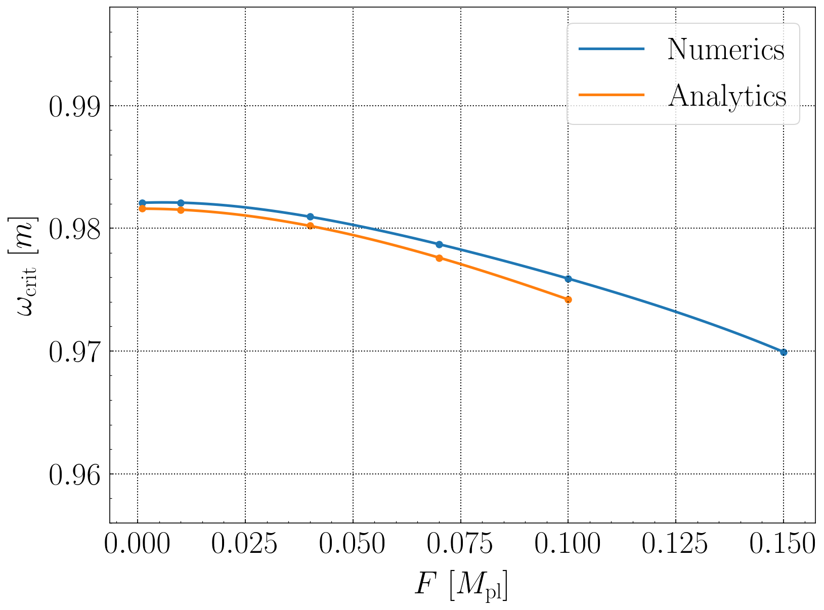
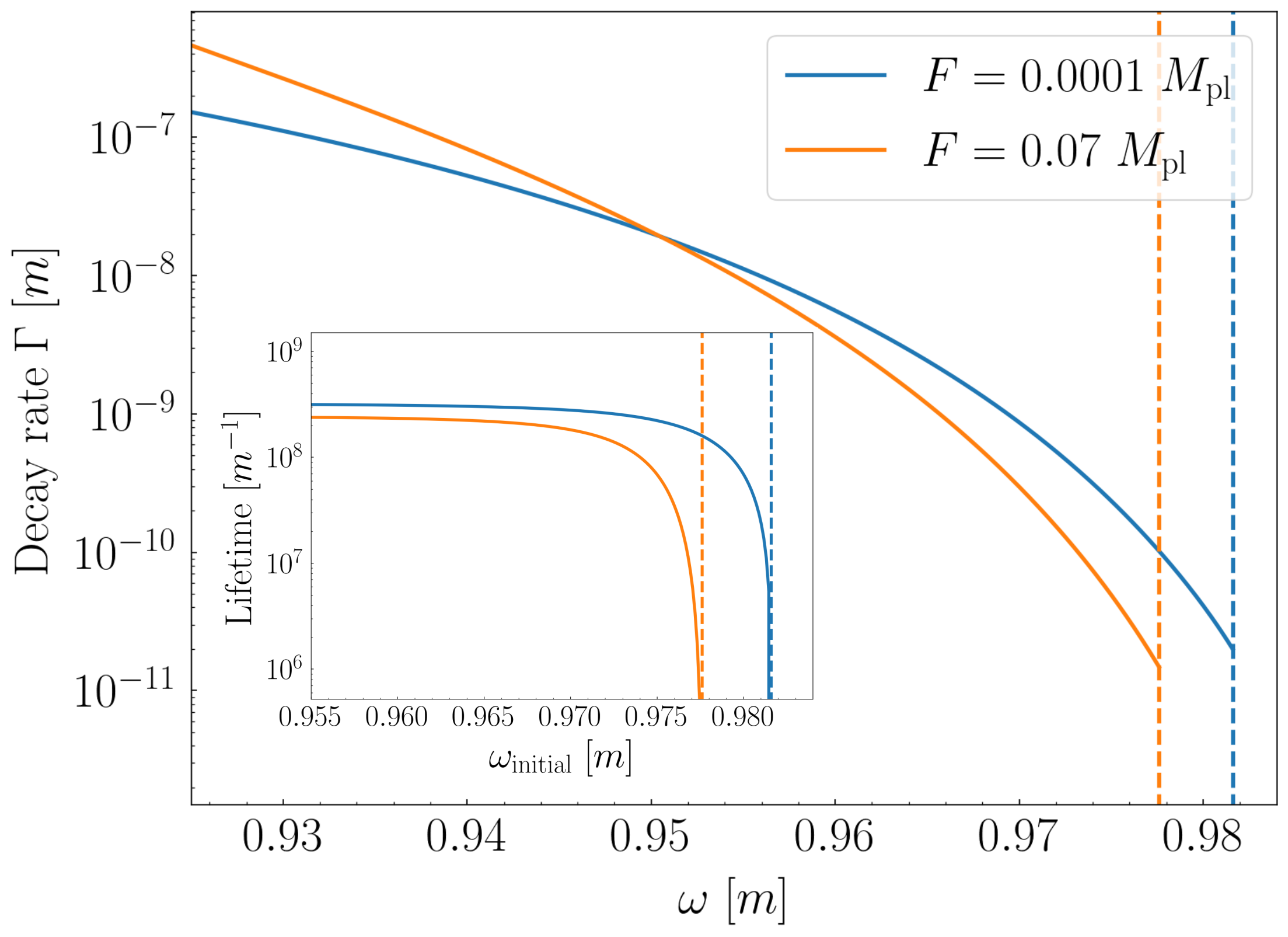
Figure 4: Two determinant factors of oscillon lifetimes in the axion monodromy model, values of the critical frequency (left panel) and decay rates around $\omega_{\mathrm{crit}}$ (right panel). It is shown that gravitational effects decrease the value of $\omega_{\mathrm{crit}}$, which tends to reduce the lifetime, while suppressing the decay rate around $\omega_{\mathrm{crit}}$, which tends to stablize oscillons. In the inset, we show that oscillon lifetimes are reduced slightly for the stronger-field gravity.

6 Conclusions

In this paper we generalize the method developed in our previous work Zhang:2020bec to include gravitational interactions, by expanding equations in terms of five small parameters

$$\epsilon_{r}\sim\frac{\partial_{r}^{2}}{m^{2}}~{},\quad\epsilon_{V}\sim\frac{V_{\mathrm{nl}}}{m^{2}\phi_{\mathrm{osc}}^{2}}~{},\quad\epsilon_{\xi}\sim\frac{\xi}{\phi_{\mathrm{osc}}}~{},\quad\epsilon_{\phi}\sim\frac{\phi_{\mathrm{osc}}}{M_{\mathrm{pl}}}~{},\quad\epsilon_{g}\sim\Phi~{},$$ (70)

where $\epsilon_{r}\sim-\epsilon_{V}\sim\epsilon_{\xi}$ and $\epsilon_{g}\sim\epsilon_{\phi}^{2}/\epsilon_{r}$ for dense oscillons. We have shown in Zhang:2020bec that keeping just the leading order of $\epsilon_{r},\epsilon_{V}$ and $\epsilon_{\xi}$ gives accurate predictions of oscillon decay rates and lifetimes in Minkowski spacetime. Thus in this paper, we explore the impacts of $\epsilon_{\phi}$ and $\epsilon_{g}$ by keeping all other parameters fixed. The application of our semi-analytical and perturbative framework is based on two assumptions, the non-relativistic limit of oscillons and the weak-field limit of gravity, namely $\epsilon_{r}\lesssim 0.1$ and $\epsilon_{\phi}\lesssim 0.1$.

In order to explore the gravitational effects on oscillon lifetimes, we discuss two well-motivated and representative models in detail, the $\alpha$-attractor T-model of inflation and the axion monodromy model with potentials given by (1). As presented in figure 2, 3 and 4, our results for $F\sim 0.1M_{\mathrm{pl}}$ show the following:

• In the $\alpha$-attractor T-model, oscillon lifetimes are dominated by an exceptionally stable intermediate configuration, which is visualized as a dip structure in figure 1. We show that the existence of gravity decreases the value of $\omega_{\rm dip}$ and increases the decay rate at $\omega_{\rm dip}$. As a result, oscillon lifetimes are reduced when gravity becomes more important.

• In the axion monodromy model, oscillons are the most stable just before their final collapse at $\omega_{\mathrm{crit}}$. It is shown that stronger gravitational effects suppress the decay rate around $\omega_{\mathrm{crit}}$, which tends to stablize oscillons, while diminishing the value of $\omega_{\mathrm{crit}}$, which tends to decrease the lifetime. By explicitly integrating out the decay rate, we find that the latter factor dominates and oscillon lifetimes are reduced slightly.

In both examples we have considered, the evolution of an oscillon is almost identical to that in Minkowski spacetime if $F\ll 0.1M_{\mathrm{pl}}$. Therefore, in such cases, one may study the decay rate and dynamics of at least single oscillons by ignoring gravity.

For stronger-field gravity, i.e. $\epsilon_{\phi}\gtrsim 0.1$ or $F\gtrsim 0.1M_{\mathrm{pl}}$, our equations with leading-order corrections are no longer accurate. Also note that both $\epsilon_{\phi}$ and $\epsilon_{g}$ increase rapidly when we probe smaller frequences. Thus one should keep higher-order perturbations of $\epsilon_{\phi}$ and $\epsilon_{g}$ to obtain more reliable conclusions. But in this regime, exotic phenomena such as black hole formation Helfer:2016ljl ; Muia:2019coe ; Nazari:2020fmk might be more interesting than oscillon lifetimes. In future work, we will further show that a new phenomenon of migration from dense to dilute oscillons makes the notion of oscillon lifetimes less meaningful.

Appendix A Fourier cosine coefficients of scalar potentials

In order to build some intuition of how $U_{j},J_{j}$ and $M_{j}$ behave, let us consider a symmetric polynomial potential of the general form

$$V_{\mathrm{nl}}(\phi)=\sum_{n=4}^{\infty}\frac{g_{n}}{n!}\phi^{n}~{},$$ (71)

where $n$ is even. By using the oscillon profile $\phi_{\mathrm{osc}}=\phi_{1}\cos(\omega t)$ and the identity

$$\cos^{n}(\omega t)=\sum_{k=0}^{n}\frac{1}{2^{n}}\frac{n!}{(n-k)!k!}\cos[(n-2k)\omega t]~{},$$ (72)

we find the potentials can be written in terms of Fourier cosine series

$$U= \sum_{n=4}^{\infty}\frac{g_{n}}{2^{n}\left(\frac{n}{2}!\right)^{2}}\phi_{1}^{n}+\sum_{n=4}^{\infty}\frac{g_{n}}{2^{n-1}\left(\frac{n+2}{2}\right)!\left(\frac{n-2}{2}\right)!}\phi_{1}^{n}\cos(2\omega t)$$ (73)

$$+\sum_{j=4}^{\infty}\sum_{n=j}^{\infty}\frac{g_{n}}{2^{n-1}\left(\frac{n+j}{2}\right)!\left(\frac{n-j}{2}\right)!}\phi_{1}^{n}\cos(j\omega t)~{},$$ (74)

$$M= \sum_{n=2}^{\infty}\frac{g_{n+2}}{2^{n}\left(\frac{n}{2}!\right)^{2}}\phi_{1}^{n}+\sum_{j=2}^{\infty}\sum_{n=j}^{\infty}\frac{g_{n+2}}{2^{n-1}\left(\frac{n+j}{2}\right)!\left(\frac{n-j}{2}\right)!}\phi_{1}^{n}\cos(j\omega t)~{},$$ (75)

where $j$ and $n$ are even, and

$$J=\sum_{n=3}^{\infty}\frac{g_{n+1}}{2^{n-1}\left(\frac{n+1}{2}\right)!\left(\frac{n-1}{2}\right)!}\phi_{1}^{n}\cos(\omega t)+\sum_{j=3}^{\infty}\sum_{n=j}^{\infty}\frac{g_{n+1}}{2^{n-1}\left(\frac{n+j}{2}\right)!\left(\frac{n-j}{2}\right)!}\phi_{1}^{n}\cos(j\omega t)~{},$$ (76)

where $j$ and $n$ are odd.

Appendix B Numerical algorithms

In this appendix we introduce briefly our numerical algorithm. For convenience we will set $M_{\mathrm{pl}}\equiv 1$ so that all the mass is in unit of reduced Planck mass. And to make the equations more accessible to coding, define

$$A\equiv e^{-\Psi}~{},\quad B\equiv e^{\Phi+\Psi}~{},\quad v\equiv B^{-1}\phi_{,0}~{},\quad u\equiv\phi_{,1}~{}.$$ (77)

Then the equation of motion of $\phi$ becomes

$$\phi_{,0}=vB~{},\quad u_{,0}=(vB)_{,1}~{},\quad v_{,0}=r^{-2}(r^{2}Bu)_{,1}-A^{2}BV^{\prime}(\phi)~{},$$ (78)

where the metric can be given by 00 and 11 components of Einstein equations, i.e.

$$A_{,1} =\frac{A}{2}\left[\frac{1-A^{2}}{r}+\frac{r}{2}\left(v^{2}+u^{2}+2A^{2}V\right)\right]~{},$$ (79)

$$B_{,1} =B\left(\frac{A^{2}-1}{r}-rA^{2}V\right)~{}.$$ (80)

One is also recommended to rescale the fields in unit of $F$ to reduce the roundoff errors brought by small numbers when $F\ll M_{\mathrm{pl}}$. The oscillon energy can be calculated by

$$E_{\mathrm{osc}}=\int_{0}^{\infty}\frac{1}{2}B(v^{2}+u^{2}+2A^{2}V)~{}4\pi r^{2}dr~{}.$$ (81)

To maintain the smoothness at the center $r=0$, we must require

$$u=v_{,1}=0~{},\quad A=1~{},\quad A_{,1}=B_{,1}=0~{}.$$ (82)

To appropriately account for the origin, we set a spatial grid $r_{n}=(n-1/2)dr$ with a fictitious point $r_{0}=-dr/2$. The inner boundary conditions then become a parity condition: $\phi,v,A,B$ are even and $u$ is odd. For the outer boundary conditions we adopt the radiative boundary conditions Alcubierre:2000xu by assuming that the dynamical variables $\phi$ and $v$ behave like spherical waves $\phi(t,r)=f(r-t)/r$. In practice, we will use this in the differential form

$$\phi_{,0}+\phi_{,1}+\phi/r=0~{},\quad v_{,0}+v_{,1}+v/r=0~{},\quad v+u+\phi/r=0~{},$$ (83)

for $\phi,v,u$ repectively. Note that one actually does not need boundary conditions for $\phi$, but we find that integrating $\phi$ all the way to the boundary point will inevitably generate instabilities in long-time simulations. Finally, we note that the Schwarzchild metric should be recovered at large $r$ hence $A$ and $B$ satisfy

$$B(r\rightarrow\infty)=1/A^{2}(r\rightarrow\infty)~{}.$$ (84)

We adopt 4th-order Runge-Kutta method as the time integrator to evolve equations (78), while the spatial derivatives are discretized by the standard 4th-order centered difference Zlochower:2005bj . The 6th-order Kreiss-Oliger dissipation with strength parameter $\epsilon=0.001$ alcubierre2008introduction is added except boundary points to avoid shock waves while the accuracy is still remained. The boundary condition (83) is discretized by finite difference methods, specifically a 2nd-order upwind method alcubierre2008introduction

$$v^{m+1}_{n}=\frac{1}{1+dt/dr}\left[\left(1-\frac{dt}{dr}-\frac{2dt}{r_{n}}\right)v^{m}_{n}+\left(1+\frac{dt}{dr}\right)v^{m}_{n-1}-\left(1-\frac{dt}{dr}\right)v^{m+1}_{n-1}\right]~{},$$ (85)

where $m,n$ are the temporal and spatial indices respectively. Once $\phi,u,v$ have been advanced for one time level, we use the 4th-order Runge-Kutta method to integrate (79) outwards and (80) inwards to get $A,B$. The initial values of $B$ are obtained by using the Schwarzchild condition (84).

We typically set the boundary at a finite value $r_{f}$, which should be significantly larger than the oscillon size, and $dr=2dt$ to satisfy the Courant-Friedrichs-Lewy condition. All the physical quantities are averaged over a time window $T_{\mathrm{ave}}=300~{}\mathrm{m^{-1}}$, which is much larger than one period $2\pi/\omega$ but smaller than oscillon lifetime, unless otherwise stated. We have checked that slight changes of parameters (i.e. $dt,dr,r_{f},\epsilon,T_{\mathrm{ave}}$) do not affect the results significantly.

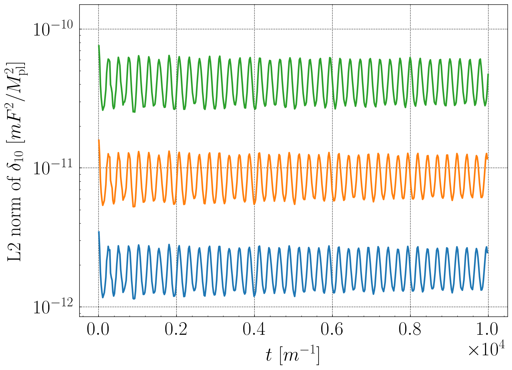
Figure 5: Convergence test for axion monodromy-type potential with $F=10^{-3}M_{\mathrm{pl}}$. Three colors refer to three different resolutions: $dt=0.025m^{-1}$ (blue), $dt=0.05m^{-1}$ (orange) and $dt=0.1m^{-1}$ (green). The initial conditions correspond to a Gaussian profile $\phi(r)=1.43F\exp(-m^{2}r^{2}/5.2^{2})$. And we have set $T_{\mathrm{ave}}=20m^{-1}$ to average the data. The fact that the L2 norm values increase by a factor of 4 every time we double the time step shows that the code maintains 2nd-order convergent.

Although we tried to implement 4th-order methods to evolve the system, the $1/r$ terms at small $r$ and the boundary discretization will destroy the 4th-order accuracy, hence we expect our algorithm to maintain 2nd-order. The codes can be tested by an exact equation

$$\delta_{10}\equiv A_{,0}-rABuv/2=0~{},$$ (86)

which is just the $10$ component of Einstein equations. As an example, we plot L2 norm of $\delta_{10}$ across the grids in figure 5, where the L2 norm is defined by $||\phi||_{2}\equiv\sqrt{\frac{1}{N}\sum_{n=0}^{N-1}\phi_{n}^{2}}$ , and $\phi_{n}$ denotes the value of $\phi$ at the spatial point $r_{n}$.

References

- (1) A. E. Kudryavtsev, Solitonlike solutions for a higgs scalar field, JETP Lett. (USSR) (Engl. Transl.), v. 22, no. 3, pp. 82-83 .
- (2) I. Bogolyubsky and V. Makhankov, Lifetime of Pulsating Solitons in Some Classical Models, Pisma Zh. Eksp. Teor. Fiz. 24 (1976) 15.
- (3) E. J. Copeland, M. Gleiser and H.-R. Muller, Oscillons: Resonant configurations during bubble collapse, Phys. Rev. D 52 (1995) 1920 [hep-ph/9503217].
- (4) M. A. Amin and D. Shirokoff, Flat-top oscillons in an expanding universe, Phys. Rev. D81 (2010) 085045 [1002.3380].
- (5) M. A. Amin, K-oscillons: Oscillons with noncanonical kinetic terms, Phys. Rev. D87 (2013) 123505 [1303.1102].
- (6) E. Seidel and W.-M. Suen, Formation of solitonic stars through gravitational cooling, Phys. Rev. Lett. 72 (1994) 2516 [gr-qc/9309015].
- (7) E. Farhi, N. Graham, A. H. Guth, N. Iqbal, R. Rosales and N. Stamatopoulos, Emergence of Oscillons in an Expanding Background, Phys. Rev. D 77 (2008) 085019 [0712.3034].
- (8) M. A. Amin, Inflaton fragmentation: Emergence of pseudo-stable inflaton lumps (oscillons) after inflation, 1006.3075.
- (9) D. Levkov, A. Panin and I. Tkachev, Gravitational Bose-Einstein condensation in the kinetic regime, Phys. Rev. Lett. 121 (2018) 151301 [1804.05857].
- (10) M. A. Amin, R. Easther and H. Finkel, Inflaton Fragmentation and Oscillon Formation in Three Dimensions, JCAP 1012 (2010) 001 [1009.2505].
- (11) M. A. Amin, R. Easther, H. Finkel, R. Flauger and M. P. Hertzberg, Oscillons After Inflation, Phys. Rev. Lett. 108 (2012) 241302 [1106.3335].
- (12) K. D. Lozanov and M. A. Amin, End of inflation, oscillons, and matter-antimatter asymmetry, Phys. Rev. D 90 (2014) 083528 [1408.1811].
- (13) K. D. Lozanov and M. A. Amin, Equation of State and Duration to Radiation Domination after Inflation, Phys. Rev. Lett. 119 (2017) 061301 [1608.01213].
- (14) K. D. Lozanov and M. A. Amin, Self-resonance after inflation: oscillons, transients and radiation domination, Phys. Rev. D97 (2018) 023533 [1710.06851].
- (15) X.-X. Kou, C. Tian and S.-Y. Zhou, Oscillon Preheating in Full General Relativity, 1912.09658.
- (16) J. Ollé, O. Pujolàs and F. Rompineve, Oscillons and Dark Matter, 1906.06352.
- (17) M. A. Amin and P. Mocz, Formation, gravitational clustering, and interactions of nonrelativistic solitons in an expanding universe, Phys. Rev. D 100 (2019) 063507 [1902.07261].
- (18) A. Arvanitaki, S. Dimopoulos, M. Galanis, L. Lehner, J. O. Thompson and K. Van Tilburg, The Large-Misalignment Mechanism for the Formation of Compact Axion Structures: Signatures from the QCD Axion to Fuzzy Dark Matter, 1909.11665.
- (19) M. Kawasaki, W. Nakano, H. Nakatsuka and E. Sonomoto, Oscillons of Axion-Like Particle: Mass distribution and power spectrum, 2010.09311.
- (20) I. Dymnikova, L. Koziel, M. Khlopov and S. Rubin, Quasilumps from first order phase transitions, Grav. Cosmol. 6 (2000) 311 [hep-th/0010120].
- (21) M. Gleiser, N. Graham and N. Stamatopoulos, Long-Lived Time-Dependent Remnants During Cosmological Symmetry Breaking: From Inflation to the Electroweak Scale, Phys. Rev. D 82 (2010) 043517 [1004.4658].
- (22) J. R. Bond, J. Braden and L. Mersini-Houghton, Cosmic bubble and domain wall instabilities III: The role of oscillons in three-dimensional bubble collisions, JCAP 09 (2015) 004 [1505.02162].
- (23) S.-Y. Zhou, E. J. Copeland, R. Easther, H. Finkel, Z.-G. Mou and P. M. Saffin, Gravitational Waves from Oscillon Preheating, JHEP 10 (2013) 026 [1304.6094].
- (24) T. Helfer, E. A. Lim, M. A. Garcia and M. A. Amin, Gravitational Wave Emission from Collisions of Compact Scalar Solitons, Phys. Rev. D 99 (2019) 044046 [1802.06733].
- (25) J. Liu, Z.-K. Guo, R.-G. Cai and G. Shiu, Gravitational Waves from Oscillons with Cuspy Potentials, Phys. Rev. Lett. 120 (2018) 031301 [1707.09841].
- (26) M. A. Amin, J. Braden, E. J. Copeland, J. T. Giblin, C. Solorio, Z. J. Weiner et al., Gravitational waves from asymmetric oscillon dynamics?, Phys. Rev. D 98 (2018) 024040 [1803.08047].
- (27) K. D. Lozanov and M. A. Amin, Gravitational perturbations from oscillons and transients after inflation, Phys. Rev. D99 (2019) 123504 [1902.06736].
- (28) T. Dietrich, F. Day, K. Clough, M. Coughlin and J. Niemeyer, Neutron star–axion star collisions in the light of multimessenger astronomy, Mon. Not. Roy. Astron. Soc. 483 (2019) 908 [1808.04746].
- (29) A. Hook, Y. Kahn, B. R. Safdi and Z. Sun, Radio Signals from Axion Dark Matter Conversion in Neutron Star Magnetospheres, Phys. Rev. Lett. 121 (2018) 241102 [1804.03145].
- (30) K. Clough, T. Dietrich and J. C. Niemeyer, Axion star collisions with black holes and neutron stars in full 3D numerical relativity, Phys. Rev. D 98 (2018) 083020 [1808.04668].
- (31) D. Levkov, A. Panin and I. Tkachev, Radio-emission of axion stars, Phys. Rev. D 102 (2020) 023501 [2004.05179].
- (32) A. Prabhu and N. M. Rapidis, Resonant Conversion of Dark Matter Oscillons in Pulsar Magnetospheres, 2005.03700.
- (33) M. A. Amin and Z.-G. Mou, Electromagnetic Bursts from Mergers of Oscillons in Axion-like Fields, 2009.11337.
- (34) M. Kawasaki, W. Nakano, H. Nakatsuka and E. Sonomoto, Probing Oscillons of Ultra-Light Axion-like Particle by 21cm Forest, 2010.13504.
- (35) T. Helfer, D. J. E. Marsh, K. Clough, M. Fairbairn, E. A. Lim and R. Becerril, Black hole formation from axion stars, JCAP 03 (2017) 055 [1609.04724].
- (36) F. Muia, M. Cicoli, K. Clough, F. Pedro, F. Quevedo and G. P. Vacca, The Fate of Dense Scalar Stars, JCAP 07 (2019) 044 [1906.09346].
- (37) Z. Nazari, M. Cicoli, K. Clough and F. Muia, Oscillon collapse to black holes, 2010.05933.
- (38) J. Y. Widdicombe, T. Helfer and E. A. Lim, Black hole formation in relativistic Oscillaton collisions, JCAP 01 (2020) 027 [1910.01950].
- (39) M. Khlopov, B. Malomed and I. Zeldovich, Gravitational instability of scalar fields and formation of primordial black holes, Mon. Not. Roy. Astron. Soc. 215 (1985) 575.
- (40) E. Cotner, A. Kusenko and V. Takhistov, Primordial Black Holes from Inflaton Fragmentation into Oscillons, Phys. Rev. D98 (2018) 083513 [1801.03321].
- (41) E. Cotner, A. Kusenko, M. Sasaki and V. Takhistov, Analytic Description of Primordial Black Hole Formation from Scalar Field Fragmentation, JCAP 10 (2019) 077 [1907.10613].
- (42) H. Segur and M. D. Kruskal, Nonexistence of Small Amplitude Breather Solutions in Theory, Phys. Rev. Lett. 58 (1987) 747.
- (43) G. Fodor, P. Forgacs, Z. Horvath and M. Mezei, Computation of the radiation amplitude of oscillons, Phys. Rev. D 79 (2009) 065002 [0812.1919].
- (44) M. P. Hertzberg, Quantum Radiation of Oscillons, Phys. Rev. D82 (2010) 045022 [1003.3459].
- (45) K. Mukaida, M. Takimoto and M. Yamada, On Longevity of I-ball/Oscillon, JHEP 03 (2017) 122 [1612.07750].
- (46) M. Ibe, M. Kawasaki, W. Nakano and E. Sonomoto, Decay of I-ball/Oscillon in Classical Field Theory, JHEP 04 (2019) 030 [1901.06130].
- (47) H.-Y. Zhang, M. A. Amin, E. J. Copeland, P. M. Saffin and K. D. Lozanov, Classical Decay Rates of Oscillons, JCAP 07 (2020) 055 [2004.01202].
- (48) P. Grandclement, G. Fodor and P. Forgacs, Numerical simulation of oscillatons: extracting the radiating tail, Phys. Rev. D 84 (2011) 065037 [1107.2791].
- (49) J. Eby, P. Suranyi and L. Wijewardhana, The Lifetime of Axion Stars, Mod. Phys. Lett. A 31 (2016) 1650090 [1512.01709].
- (50) J. Eby, L. Street, P. Suranyi and L. Wijewardhana, Global View of Axion Stars with (Nearly) Planck-Scale Decay Constants, 2011.09087.
- (51) E. Seidel and W. Suen, Oscillating soliton stars, Phys. Rev. Lett. 66 (1991) 1659.
- (52) L. Urena-Lopez, T. Matos and R. Becerril, Inside oscillatons, Class. Quant. Grav. 19 (2002) 6259.
- (53) M. Alcubierre, R. Becerril, S. F. Guzman, T. Matos, D. Nunez and L. A. Urena-Lopez, Numerical studies of Phi**2 oscillatons, Class. Quant. Grav. 20 (2003) 2883 [gr-qc/0301105].
- (54) L. Visinelli, S. Baum, J. Redondo, K. Freese and F. Wilczek, Dilute and dense axion stars, Phys. Lett. B 777 (2018) 64 [1710.08910].
- (55) J. Eby, M. Leembruggen, L. Street, P. Suranyi and L. R. Wijewardhana, Global view of QCD axion stars, Phys. Rev. D 100 (2019) 063002 [1905.00981].
- (56) L. Hui, J. P. Ostriker, S. Tremaine and E. Witten, Ultralight scalars as cosmological dark matter, Phys. Rev. D 95 (2017) 043541 [1610.08297].
- (57) R. Kallosh and A. Linde, Universality Class in Conformal Inflation, JCAP 1307 (2013) 002 [1306.5220].
- (58) E. Silverstein and A. Westphal, Monodromy in the CMB: Gravity Waves and String Inflation, Phys. Rev. D78 (2008) 106003 [0803.3085].
- (59) L. McAllister, E. Silverstein, A. Westphal and T. Wrase, The Powers of Monodromy, JHEP 09 (2014) 123 [1405.3652].
- (60) A. H. Guth, M. P. Hertzberg and C. Prescod-Weinstein, Do Dark Matter Axions Form a Condensate with Long-Range Correlation?, Phys. Rev. D 92 (2015) 103513 [1412.5930].
- (61) M. Hindmarsh and P. Salmi, Numerical investigations of oscillons in 2 dimensions, Phys. Rev. D 74 (2006) 105005 [hep-th/0606016].
- (62) N. Sanchis-Gual, F. Di Giovanni, M. Zilhão, C. Herdeiro, P. Cerdá-Durán, J. Font et al., Nonlinear Dynamics of Spinning Bosonic Stars: Formation and Stability, Phys. Rev. Lett. 123 (2019) 221101 [1907.12565].
- (63) R. Friedberg, T. Lee and A. Sirlin, A Class of Scalar-Field Soliton Solutions in Three Space Dimensions, Phys. Rev. D 13 (1976) 2739.
- (64) T. Lee and Y. Pang, Nontopological solitons, Phys. Rept. 221 (1992) 251.
- (65) G. Gibbons and S. Hawking, Action Integrals and Partition Functions in Quantum Gravity, Phys. Rev. D 15 (1977) 2752.
- (66) T. D. Lee and Y. Pang, Stability of Mini-Boson Stars, Nucl. Phys. B 315 (1989) 477.
- (67) R. L. Arnowitt, S. Deser and C. W. Misner, The Dynamics of general relativity, Gen. Rel. Grav. 40 (2008) 1997 [gr-qc/0405109].
- (68) J. Eby, K. Mukaida, M. Takimoto, L. C. R. Wijewardhana and M. Yamada, Classical nonrelativistic effective field theory and the role of gravitational interactions, Phys. Rev. D99 (2019) 123503 [1807.09795].
- (69) E. Braaten, A. Mohapatra and H. Zhang, Classical Nonrelativistic Effective Field Theories for a Real Scalar Field, Phys. Rev. D 98 (2018) 096012 [1806.01898].
- (70) M. H. Namjoo, A. H. Guth and D. I. Kaiser, Relativistic Corrections to Nonrelativistic Effective Field Theories, Phys. Rev. D 98 (2018) 016011 [1712.00445].
- (71) B. Salehian, M. H. Namjoo and D. I. Kaiser, Effective theories for a nonrelativistic field in an expanding universe: Induced self-interaction, pressure, sound speed, and viscosity, 2005.05388.
- (72) R. Friedberg, T. Lee and Y. Pang, MINI - SOLITON STARS, Phys. Rev. D 35 (1987) 3640.
- (73) M. Alcubierre, G. Allen, B. Bruegmann, T. Dramlitsch, J. A. Font, P. Papadopoulos et al., Towards a stable numerical evolution of strongly gravitating systems in general relativity: The Conformal treatments, Phys. Rev. D62 (2000) 044034 [gr-qc/0003071].
- (74) Y. Zlochower, J. Baker, M. Campanelli and C. Lousto, Accurate black hole evolutions by fourth-order numerical relativity, Phys. Rev. D 72 (2005) 024021 [gr-qc/0505055].
- (75) M. Alcubierre, Introduction to 3+ 1 numerical relativity, vol. 140. Oxford University Press, 2008.