DeepClimGAN: A High-Resolution Climate Data Generator

1 Introduction

Earth system models (ESMs), which simulate the physics and chemistry of the global atmosphere, land, and ocean, are often used to generate future projections of climate change scenarios. These models are far too computationally intensive to run repeatedly, but limited sets of runs are insufficient for some important applications, like adequately sampling distribution tails to characterize extreme events. As a compromise, emulators are substantially less expensive but may not have all of the complexity of an ESM. Here we demonstrate the use of a conditional generative adversarial network (GAN) to act as an ESM emulator. In doing so, we gain the ability to produce daily weather data that is consistent with what ESM might output over any chosen scenario. In particular, the GAN is aimed at representing a joint probability distribution over space, time, and climate variables, enabling the study of correlated extreme events, such as floods, droughts, or heatwaves.

The use of neural networks in weather forecasting predates the deep learning boom (Hall et al., 1999; Koizumi, 1999). Shi et al. (2015) introduced convolutional LSTMs for the task of precipitation nowcasting; we plan to incorporate elements from their architecture into our design. Dueben & Bauer (2018) and Schneider et al. (2017) both present important considerations and challenges in weather and climate modeling with machine learning. Wu et al. (2019) present a strategy for incorporating constraints into GANs that are applicable to our task. Rasp et al. (2018) and Brenowitz & Bretherton (2018) both demonstrate that deep learning can be used to accurate model subgrid processes in climate tasks. Neither use GANs, but Rasp et al. (2018) expresses optimism about their potential. Both Weber et al. (2019) and Lu & Ricciuto (2019) tackle efficient surrogate modeling, and find deep learning to be effective.

2 High-Resolution Climate Data Generation

2.1 The DeepClimGAN

Generative Adversarial Networks (GANs) (Goodfellow et al., 2014) have been rapidly and widely adopted for the generation of realistic images. They leverage two competing architectures: the generator and the discriminator. The networks are trained jointly in a minimax fashion, ideally reaching an equilibrium in which samples from the two distributions are indistinguishable and the discriminator cannot exceed 50% accuracy. GANs have had widespread success in image and video applications, making them a promising choice for generating gridded climate data.

DeepClimGAN is a conditional GAN, capable of producing a spatio-temporal forecast, generating samples $y\in\mathbb{R}^{H\times W\times T\times V}$, where the spatial dimensions are $H$ and $W$, the temporal dimension is $T$, and there are $V$ real-valued climate variables predicted at each location and time. For simplicity, we set $T=32$ for a convenient “month-like” forecast period. The $V=7$ climate variables we use in this work are: $\{$ min, avg, max $\}$ temperature, $\{$ min, avg, max $\}$ relative humidity, and precipitation; we chose these variables because those are the variables required by various impact models, including hydrology, agriculture and health (e.g. heat index). A high-resolution generator for these variables would enable new insights into climate impacts and risks faced by human systems.

Each sample is conditioned on some context, $c$. This conditioning information should capture the initial state from the start of the forecast and the constraints we want our forecast to observe. Therefore, we assume that $c$ consists of two components: 1) “monthly” context $c_{1}\in\mathbb{R}^{H\times W\times 2}$, containing the average precipitation and temperature for the month (length $T$ period), and 2) recent context $c_{2}\in\mathbb{R}^{H\times W\times KV}$, containing all $V$ climate variables for the $K$ days immediately preceding the month, stacked. The the $c_{1}$ information allows us to specify the type of scenario (e.g. high or low warming) we wish to generate, while the $c_{2}$ information allows us to ensure continuity between months.

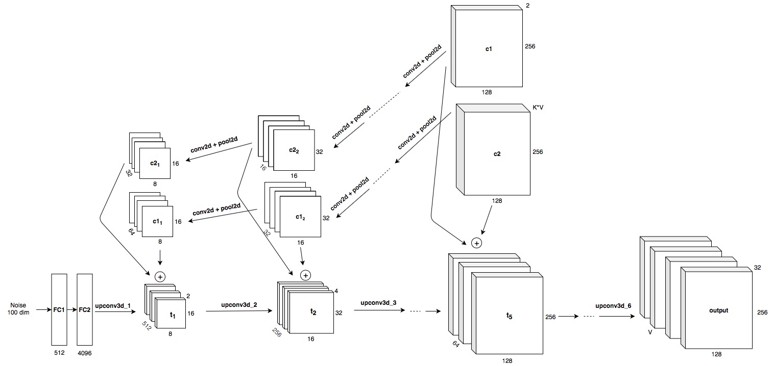
Figure 1: Generator.

The generator and discriminator architectures, including conditioning subarchitectures, are shown in Figures 1 and 2, respectively, and described below. Both architectures were inspired by the work of Vondrick et al. (2016) on video generation with GANs.

Generator

As shown in the bottom track of Fig. 1, the base generator projects noise $z\in\mathbb{R}^{100}$ to $\mathbb{R}^{4096}$ via two fully connected layers; it is then reshaped and fed through a series of six 3d up (transposed) convolutions. After all but the last layer, we apply batch normalization (Ioffe & Szegedy, 2015) followed by a ReLU activation function. For the output layer, we apply ReLU only to the precipitation channel to, avoid predicting negative precipitation, while still allowing precipitation-free days. Additionally, we pass the mean, maximum and minimum relative humidity through a logistic sigmoid to constrain them to be in $(0,1)$.

As described above, we incorporate two forms of context: low resolution monthly totals $c_{1}$, and a high resolution initial condition $c_{2}$. These contexts are injected at each convolutional layer into the base generator. The original contexts $c_{1}$ and $c_{2}$ are spatially downsampled through a series of 2d convolutional and $2\times 2$ maxpool layers. We replicate the 2d contexts across the time dimension and then append along the channel dimension so that it serves as additional input to each 3d up convolution. The end result, in the lower right of Fig. 1, is our spatio-temporal forecast for all $V$ climate variables.

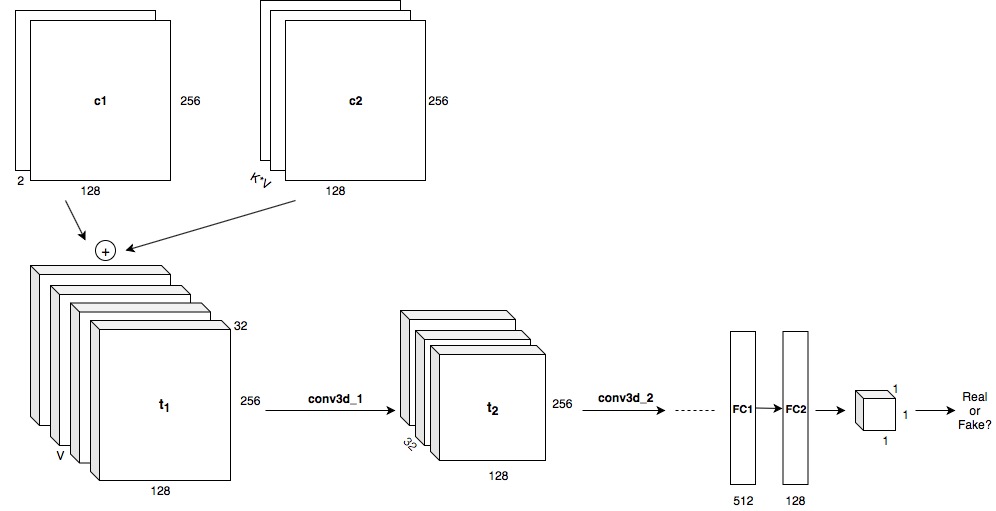
Figure 2: Discriminator.

Discriminator

The discriminator, shown in Fig. 2, consists of four 3d convolution layers followed by two fully connected layers. Each layer is followed by batch normalization (Ioffe & Szegedy, 2015) and leaky ReLU (Xu et al., 2015). The output activation is logistic sigmoid, yielding a scalar probability of the data being real (i.e., instead of generated). Conditioning is accomplished by appending the context along the channel dimension of the input.

Training

We train the model with alternating updates for generator and discriminator. Our true examples are 32 day periods with randomly sampled start days. The high resolution context ($c_{2}$) is the five days prior to the sampled month. The low resolution context is produced by averaging precipitation and temperature over the 32 day period. The model is implemented in PyTorch, based on a model described in Vondrick et al. (2016). We use Adam (Kingma & Ba, 2014) to optimize the model. The learning rate is fixed at 0.0002 with a momentum of 0.5 and a batch size of 32. We initialize all weights with zero mean Gaussian noise with standard deviation 0.02. To improve training, we have explored 1) adding Gaussian noise to the real and generated data before feeding to the discriminator, 2) adding an experience replay mechanism, in which previously generated samples are stored and also fed to the discriminator, and 3) pretraining the generator to produce similar marginal temperature and precipitation statistics as ground truth data.

2.2 Generation with the DeepClimGAN

We generate high-resolution weather arbitrarily far into the future as follows:

1. Run a low-resolution ESM emulator to produce monthly contexts ($c_{1}s$) for as many future months as desired.

2. Sample month 1’s weather from the generator, conditioned on $K$ days of ground truth $c_{2}$ and the first month’s low resolution context $c_{1}$.

3. For $i=2\ldots N$: take the last $K$ days of the previous month’s generated data as the new $c_{2}$, input the corresponding $c_{1}$ from the low-resolution emulator and sample month $i$’s weather from the generator.

The rationale for using the initial state context is that it allows us to maintain continuity: when we chain several months of generated data together, conditioning on the last few days of the previous month allows us to avoid having statistical artifacts at the month boundary.

3 Experiments and Initial Findings

3.1 Data

We used daily resolution CMIP5 (“Coupled Model Intercomparison Project, Phase 5”) (Taylor et al., 2011) archival data for the MIROC5 model (Watanabe et al., 2010) under different greenhouse gas emission scenarios. The scenarios provided by the model span: pre-industrial (idealized, constant 1860 conditions, run for 200 years), historical (1861-2005), future (2006-2099), and extended future (2100-2299). Each scenario is represented in several realizations (simulations with different initial conditions to capture a range of internal variability). Details of the source data are provided in Table 1 in Appendix B. DeepClimGAN is agnostic to the model it emulates: swapping the training data should result in a generator that can approximate the desired data distribution. We selected 1680 years of data for training. A daily map for each of the climate variables is represented in 128 $\times$ 256 spatial resolution. We applied $\log(1+x)$-normalization for precipitation, mapped relative humidity into $(0,1)$ and standardized the temperature variables.

3.2 Initial Findings

Figure 3: Histogram of real vs generated daily avg. temperature.

Figures 3 and 4 show the results of initial experiments, with a model that includes pretraining as described in Sec. 2. Fig. 3 shows histograms of temperature over 320 randomly sampled 32-day periods, contrasting ground truth with generator output. Fig. 4 shows real and generated daily temperatures for one 32 day period, for six spatial locations, each belonging to a distinct region. Both figures suggest that the generator is capable of generating fairly realistic daily average temperature values.

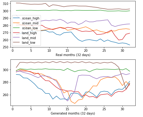
Figure 4: Real (top) and generated (bottom) daily temperature (K).

4 Future Work

Our initial findings are encouraging, but there remains a great deal of important work for this on-going project. First, we must continue to develop and refine evaluation metrics for this task. While evaluating GANs is notoriously challenging, our use case opens the door to some promising approaches. In addition to the ideas discussed in Appendix A, we will explore ways to quantify the generation quality for downstream applications (e.g. characterizing extreme events). Second, extensive experimentation is needed in order to assess the model’s ability to model the distributions induced by different climate emulators and climate change scenarios. Third, there are other promising architectures to be considered for the discriminator and generator, including those based on convolutional LSTMs. Fourth, there is rich literature of techniques we plan to draw from to improve the generative quality of our GANs (e.g. label smoothing, historical averaging, modified cost functions). Finally, we plan to generate datasets and disseminate both the data and DeepClimGAN tool to facilitate climate change research.

Appendix A: Evaluation Metrics

Evaluating GANs is notoriously difficult. For our task, we need to show that the joint probability distribution of ESM outputs is the same as joint probability distribution of the generator outputs, which requires a statistic that measures the discrepancy between the two distributions. Of that statistic, we first need to know its statistical distribution when the ESM and generator distributions are the same, which is the “null-hypothesis distribution” for the statistic. Second, we need to know how the statistic is distributed in the presence of some de minimus discrepancy (i.e., a discrepancy small enough that even if we knew it was present, we would still be willing to use the model) between the ESM and generator distributions. We use that to compute the power of our statistical test. If the power of the test is high, and the test fails to reject the null hypothesis, then we can conclude with high confidence that the two distributions are the same. We are exploring Maximum Mean Discrepancy (MMD) (Sutherland et al., 2016) and Mean Embeddings (ME) (Jitkrittum et al., 2016) metrics for evaluation of the model.

Appendix B: Dataset Details

Table 1: MIROC5 data for the model

Scenario	Realizations	Years
Historical	r1i1p1-r5i1p1	1950-2009
RCP{2.6, 4.5, 6.0, 8.5}	r1i1p1-r3i1p1	2006-2100
RCP{2.6, 4.5, 6.0, 8.5}	r4i1p1-r5i1p1	2006-2035

References

- Brenowitz & Bretherton (2018) Brenowitz, N. and Bretherton, C. Prognostic validation of a neural network unified physics parameterization. 05 2018. doi: 10.31223/osf.io/eu3ax.
- Dueben & Bauer (2018) Dueben, P. D. and Bauer, P. Challenges and design choices for global weather and climate models based on machine learning. Geoscientific Model Development, 11(10):3999–4009, 2018. doi: 10.5194/gmd-11-3999-2018.
- Goodfellow et al. (2014) Goodfellow, I. J., Pouget-Abadie, J., Mirza, M., Xu, B., Warde-Farley, D., Ozair, S., Courville, A., and Bengio, Y. Generative Adversarial Networks. arXiv e-prints, art. arXiv:1406.2661, Jun 2014.
- Hall et al. (1999) Hall, T., Brooks, H., and Doswell III, C. Precipitation forecasting using a neural network. Weather and Forecasting - WEATHER FORECAST, 14, 06 1999. doi: 10.1175/1520-0434(1999)0140338:PFUANN2.0.CO;2.
- Ioffe & Szegedy (2015) Ioffe, S. and Szegedy, C. Batch Normalization: Accelerating Deep Network Training by Reducing Internal Covariate Shift. arXiv e-prints, art. arXiv:1502.03167, Feb 2015.
- Jitkrittum et al. (2016) Jitkrittum, W., Szabo, Z., Chwialkowski, K., and Gretton, A. Interpretable Distribution Features with Maximum Testing Power. arXiv e-prints, art. arXiv:1605.06796, May 2016.
- Kingma & Ba (2014) Kingma, D. P. and Ba, J. Adam: A Method for Stochastic Optimization. arXiv e-prints, art. arXiv:1412.6980, Dec 2014.
- Koizumi (1999) Koizumi, K. An objective method to modify numerical model forecasts with newly given weather data using an artificial neural network. Weather and Forecasting - WEATHER FORECAST, 14:109–118, 02 1999. doi: 10.1175/1520-0434(1999)0140109:AOMTMN2.0.CO;2.
- Lu & Ricciuto (2019) Lu, D. and Ricciuto, D. Efficient surrogate modeling methods for large-scale earth system models based on machine-learning techniques. Geoscientific Model Development, 12(5):1791–1807, 2019. doi: 10.5194/gmd-12-1791-2019.
- Rasp et al. (2018) Rasp, S., S. Pritchard, M., and Gentine, P. Deep learning to represent subgrid processes in climate models. Proceedings of the National Academy of Sciences, 115:201810286, 09 2018. doi: 10.1073/pnas.1810286115.
- Schneider et al. (2017) Schneider, T., Lan, S., Stuart, A., and Teixeira, J. Earth system modeling 2.0: A blueprint for models that learn from observations and targeted high-resolution simulations. Geophysical Research Letters, 08 2017. doi: 10.1002/2017GL076101.
- Shi et al. (2015) Shi, X., Chen, Z., Wang, H., Yeung, D.-Y., Wong, W.-k., and Woo, W.-c. Convolutional LSTM Network: A Machine Learning Approach for Precipitation Nowcasting. arXiv e-prints, art. arXiv:1506.04214, Jun 2015.
- Sutherland et al. (2016) Sutherland, D. J., Tung, H.-Y., Strathmann, H., De, S., Ramdas, A., Smola, A., and Gretton, A. Generative Models and Model Criticism via Optimized Maximum Mean Discrepancy. arXiv e-prints, art. arXiv:1611.04488, Nov 2016.
- Taylor et al. (2011) Taylor, K. E., Ronald, S., and Meehl, G. An overview of cmip5 and the experiment design. Bulletin of the American Meteorological Society, 93:485–498, 11 2011. doi: 10.1175/BAMS-D-11-00094.1.
- Vondrick et al. (2016) Vondrick, C., Pirsiavash, H., and Torralba, A. Generating Videos with Scene Dynamics. arXiv e-prints, art. arXiv:1609.02612, Sep 2016.
- Watanabe et al. (2010) Watanabe, M., Suzuki, T., O’ishi, R., Komuro, Y., Watanabe, S., Emori, S., Takemura, T., Chikira, M., Ogura, T., Sekiguchi, M., et al. Improved climate simulation by miroc5: mean states, variability, and climate sensitivity. Journal of Climate, 23(23):6312–6335, 2010.
- Weber et al. (2019) Weber, T., Corotan, A., Hutchinson, B., Kravitz, B., and Link, R. Technical note: Deep learning for creating surrogate models of precipitation in earth system models. Atmospheric Chemistry and Physics Discussions, pp. 1–16, 04 2019. doi: 10.5194/acp-2019-85.
- Wu et al. (2019) Wu, J.-L., Kashinath, K., Albert, A., Chirila, D., Prabhat, and Xiao, H. Enforcing Statistical Constraints in Generative Adversarial Networks for Modeling Chaotic Dynamical Systems. arXiv e-prints, art. arXiv:1905.06841, May 2019.
- Xu et al. (2015) Xu, B., Wang, N., Chen, T., and Li, M. Empirical Evaluation of Rectified Activations in Convolutional Network. arXiv e-prints, art. arXiv:1505.00853, May 2015.