P3H-20-73, TTP20-040

Abstract

We compute the relation between the pole mass and the kinetic mass of a heavy quark to three loops. Using the known relation between the pole and the $\overline{\rm MS}$ mass we obtain precise conversion relations between the $\overline{\rm MS}$ and kinetic masses. The kinetic mass is defined via the moments of the spectral function for the scattering involving a heavy quark close to threshold. This requires the computation of the imaginary part of a forward scattering amplitude up to three-loop order. We discuss in detail the expansion procedure and the reduction to master integrals. For the latter analytic results are provided. We apply our result both to charm and bottom quark masses. In the latter case we compute and include finite charm quark mass effects. Furthermore, we determine the large-$\beta_{0}$ result for the conversion formula at four-loop order. For the bottom quark we estimate the uncertainty in the conversion between the $\overline{\rm MS}$ and kinetic masses to about 15 MeV which is an improvement by a factor two to three as compared to the two-loop formula. The improved precision is crucial for the extraction of the Cabibbo-Kobayashi-Maskawa matrix element $|V_{cb}|$ at Belle II.

1 Heavy quark mass definitions

Quark masses enter the QCD Lagrangian density as free parameters and as such they have to be renormalized once higher order corrections are considered. There are two distinguished renormalization schemes, the pole (or on-shell) and the (modified) minimal subtraction scheme. The pole mass scheme (OS) has the advantage that it is based on a physical definition since it requires that, order-by-order in perturbation theory, the inverse heavy-quark propagator has a zero at the position of the pole mass. On the other hand, the minimal subtraction scheme only subtracts the divergent parts of the quantum corrections to the quark two-point function and combines them with the bare mass to arrive at the renormalized ${\rm MS}$ (or $\overline{\rm MS}$) quark mass.

In high-energy reactions it is appropriate to use the $\overline{\rm MS}$ mass, which does not suffer from intrinsic uncertainties. However, typical energy scales in $B$ meson decays are smaller than the bottom quark mass which is the reason that the $\overline{\rm MS}$ mass is less appropriate in such situations. The pole mass, on the other hand, suffers from renormalon ambiguities, which manifest themselves through an ill-behaved perturbative series. This can already be seen in the relation between the on-shell and $\overline{\rm MS}$ mass which suffers from large higher order corrections [1, 2, 3]. For example, the four-loop term in the mass relation amounts to about 100 MeV for bottom quarks [4, 5], which is much larger than the current uncertainty of the $\overline{\rm MS}$ mass as, e.g., extracted from lattice calculations or low-moment sum rules (see, e.g., Refs. [6]).

In order to combine the advantages of the two canonical mass schemes, so-called threshold masses as, e.g., the potential subtracted (PS) [7], 1S [8, 9, 10], renormalon subtracted (RS) [11] or MRS [12, 13] mass have been developed. They are of short-distance nature and are free of renormalon ambiguities, as the $\overline{\rm MS}$ mass. On the other hand, the threshold masses are suitable parameters to be used for cross sections near threshold, decay rates and heavy quark bound state properties. In this article, we concentrate on the kinetic mass [14, 15], that is defined via the so-called Small-Velocity (SV) sum rules and involves the relation between the masses of heavy quark and heavy mesons up to the kinetic energy term.

The various mass definitions can be converted into each other within perturbation theory. Such a conversion is frequently needed in practical calculations as well as in the extraction of mass values from experiments. In order to achieve high precision, it is mandatory to know the conversion relations between the different mass schemes as precisely as possible. For the most commonly used ones, their relation to the pole mass is known to next-to-next-to-next-to-leading order (N³LO) [5].

In this work, we concentrate on the kinetic mass and on the methods used in the calculation of the relation between the $\overline{\mathrm{MS}}$ and the kinetic mass to $O(\alpha_{s}^{3})$ presented in [16]. In particular, we describe our approach based on expansion by regions [17, 18] to compute the SV sum rules [19, 14] that define the kinetic mass to higher orders in $\alpha_{s}$. We give an account of the reduction to master integrals and summarize our strategies for their analytic computation at three loops. Moreover, we improve our work in [16] by including finite charm mass effects in the mass relation for the bottom quark. We also present the large-$\beta_{0}$ contribution to the conversion formula at four-loop order. Our results, available as ancillary files attached to this paper and also implemented in RunDec and CRunDec [20], allow us to carefully assess for bottom and charm quark the theoretical uncertainties in the mass scheme conversions. For the bottom quark, such uncertainty is reduced by a factor two to three compared to the two-loop estimates in Ref. [21]. Our results are crucial for future extractions of $|V_{cb}|$ from $B\to X_{c}\ell\bar{\nu}_{\ell}$ decays at Belle II, in particular to better constrain global fits of the branching ratios and the moments of inclusive semileptonic $B$ decays.

The paper is structured as follows: in the next section we motivate the definition of the kinetic mass and derive the relevant formulae that are needed for the practical calculation. In Section 3 we provide several technical details on the calculation and in Section 4 we describe the calculation of the charm quark mass effects to the bottom mass relation. We discuss our analytic three-loop results in Section 5 and the four-loop large-$\beta_{0}$ terms in Section 6. The numerical effects of the new correction terms are discussed in Section 7, with special emphasis on the charm quark effects. Finally we summarize our findings in Section 8.

In Appendix A we report the analytic expressions up to $O(\alpha_{s}^{3})$ of the HQET parameters $\overline{\Lambda},\mu_{\pi},\rho_{D}$ and $r_{E}$ computed in perturbative QCD. In Appendix B we discuss in detail the calculation of the most difficult master integral while in Appendix C we provide analytic results of auxiliary integrals which were useful in the course of our calculation.

2 Why the kinetic mass?

In this section, we first summarize the motivations behind the kinetic mass scheme and the main findings of Refs. [19, 14]. Afterwards we introduce the rigorous definition of the relation between the OS and the kinetic mass in terms of SV rum rules, and present our method for its calculation to higher orders in $\alpha_{s}$ based on the expansion by regions and in a fully covariant formalism.

The basis of the precise theoretical prediction for inclusive $B\to X_{c}\ell\bar{\nu}_{\ell}$ decays is the Heavy-Quark Expansion (HQE), which allows us to predict various observables, as the total semileptonic rate as well as the moments of differential distributions (lepton energy, hadronic energy, hadronic invariant mass, etc.), as a double expansion in $\alpha_{s}(m_{b})$ and $\Lambda_{\mathrm{QCD}}/m_{b}$. The starting point is the optical theorem which relates the decay rate to the forward matrix element of a scattering amplitude:

$$\Gamma=\frac{1}{m_{B}}\mathrm{Im}\,\int{\rm d}^{4}x\,\bra{B(p_{b})}T\{\mathcal{H}_{\mathrm{eff}}^{\dagger}(x)\mathcal{H}_{\mathrm{eff}}(0)\}\ket{B(p_{b})}\,.$$ (1)

The time-ordered product can be written in terms of an operator product expansion that allows us to write

$$\int{\rm d}^{4}x\,T\{\mathcal{H}_{\mathrm{eff}}^{\dagger}(x)\mathcal{H}_{\mathrm{eff}}(0)\}=\sum_{n,i}\frac{1}{m_{b}^{n}}\mathcal{C}_{n,i}\,\mathcal{O}_{n+3,i}\,,$$ (2)

where $\mathcal{O}_{{n},i}$ is a set (labeled by $i$) of operators of dimension $n$, and $\mathcal{C}_{n,i}$ are the Wilson coefficients calculable in perturbative QCD. Taking the forward matrix element of this expression, we obtain the decay rate in terms of the Wilson coefficients and hadronic matrix elements of the operators $\mathcal{O}_{{n},i}$ encoding the non-perturbative input into the decay rate. The general structure of the expansion for an observable ${\rm d}\Gamma$ is

$${\rm d}\Gamma={\rm d}\Gamma_{0}+{\rm d}\Gamma_{\mu_{\pi}}\frac{\mu_{\pi}^{2}}{m_{b}^{2}}+{\rm d}\Gamma_{\mu_{G}}\frac{\mu_{G}^{2}}{m_{b}^{2}}+O\left(\frac{\Lambda_{\mathrm{QCD}}^{3}}{m_{b}^{3}}\right)\,,$$ (3)

where the coefficients ${\rm d}\Gamma_{i}$ are functions of $m_{c}/m_{b}$ and have an expansion in $\alpha_{s}(m_{b})$, while $\mu_{\pi}$ and $\mu_{G}$ are dimension-full parameters of order $\Lambda_{\mathrm{QCD}}$. Since the bottom quark vector current $\bar{b}\gamma^{\mu}b$ is conserved, there are for $n=0$ only perturbative corrections, i.e., ${\rm d}\Gamma_{0}$ corresponds to the decay of a free $b$ quark. Note that there are no linear $1/m_{b}$ terms in the HQE as was shown in Refs. [22, 23, 24, 25]. The first two non-perturbative contributions, denoted by $\mu_{\pi}$ and $\mu_{G}$, emerge at order $\Lambda_{\mathrm{QCD}}^{2}/m_{b}^{2}$ and can be written in terms of two matrix elements:

$$-2M_{B}\mu_{\pi}^{2} =\bra{H_{\infty}(v)}\bar{h}_{v}\,(iD_{\perp})^{2}\,h_{v}\ket{H_{\infty}(v)}\,,$$

$$2M_{B}\mu_{G}^{2} =\bra{H_{\infty}(v)}\bar{h}_{v}\,\sigma\cdot G\,h_{v}\ket{H_{\infty}(v)}\,,$$ (4)

with $\sigma\cdot G\equiv(iD_{\perp}^{\mu})(iD_{\perp}^{\nu})(-i\sigma_{\mu\nu})$, $\sigma^{\mu\nu}=\frac{i}{2}[\gamma_{\mu},\gamma_{\nu}]$ and $iD^{\mu}=iv^{\mu}\,(iv\cdot D)+D_{\perp}^{\mu}$. In Eq. (4) $h_{v}(x)$ is the $b$ quark field in the heavy quark effective theory, $v=p_{B}/M_{B}$ is the velocity of the $B$ meson and $\ket{H_{\infty}(v)}$ is the pseudoscalar or vector meson’s state in the infinite mass limit. The parameter $\mu_{\pi}^{2}$ corresponds to the kinetic energy of the heavy quark inside the heavy meson, while $\mu_{G}^{2}$ is its chromo-magnetic moment.

The HQE has a strong dependence on the mass of the heavy quark $m_{b}$. Therefore, in order to obtain precise predictions for decay rates, the quark mass has to be carefully chosen. This choice is closely intertwined with the size of the QCD corrections to the decay rates. As already mentioned above, perturbative calculations which use the pole mass scheme are affected by the renormalon ambiguity and thus show a bad behaviour of the perturbative series. Indeed if the semileptonic width $\Gamma_{\mathrm{sl}}$ is expressed in terms of the pole mass of the $b$ quark, the expression for $\Gamma_{\mathrm{sl}}$ contains a factorially divergent series in powers of $\alpha_{s}$[1, 2, 3]:

$$\Gamma_{\mathrm{sl}}\sim\sum_{k}k!\left(\frac{\beta_{0}}{2}\frac{\alpha_{s}}{\pi}\right)^{k}.$$ (5)

However, also in the $\overline{\mathrm{MS}}$ mass scheme, the $\alpha_{s}$ corrections to the $\Gamma_{\mathrm{sl}}$ have a bad convergence. Indeed, removing the infra-red (IR) renormalons by using a short distance mass definition does not guarantee yet that we have a fast convergent perturbative series. Semileptonic decays of a heavy quark are in fact also affected by large corrections of the type $(n\alpha_{s})^{k}$, with $n=5$, which arise from the conversion of the overall factor $m_{b}^{5}$ from the pole scheme to the $\overline{\mathrm{MS}}$ scheme. Note that the $(n\alpha_{s})^{k}$ enhanced terms are not related to the running of $\alpha_{s}$ and are present even for a vanishing $\beta$ function.

A further argument against the use of the $\overline{\mathrm{MS}}$ bottom quark mass at a scale $\mu=m_{b}$ for inclusive decays is that the maximal energy of the final hadronic system is limited by $m_{b}-m_{c}$. Moreover, since the two leptons in $B\to X_{c}\ell\nu$ carry away a significant fraction of the energy, the mass scale $\mu$ to be used is even smaller. However, at such low scale the logarithmic running of the $\overline{\mathrm{MS}}$ mass is considered unphysical.

The kinetic scheme for the mass of a heavy quark, $m_{Q}^{\mathrm{kin}}$, was introduced in [19, 14] to resum in the semileptonic rate the $(n\alpha_{s})^{k}$-enhanced terms via a suitable short-distance definition. It relies on a set of QCD sum rules which hold in the so-called small velocity limit, i.e. in the limit where the three-momentum components of the final state $X_{c}=D,D^{*}$ are much smaller than $m_{b}$ and $m_{c}$ in the rest frame of the $B$ meson. The SV sum rules are relations between the physical differential rate and the parameters $\mu_{\pi}$ and $\mu_{G}$, as well as $\overline{\Lambda}$, the binding-energy of a heavy hadron. They are obtained by considering moments of the hadronic energy spectrum

$$I_{n}(\vec{q}\,^{2})=\int_{|\vec{q}\,|}^{q_{0}^{\mathrm{max}}}{\rm d}q_{0}\,\omega^{n}\,\frac{{\rm d}^{2}\Gamma_{\mathrm{sl}}}{{\rm d}q_{0}{\rm d}\vec{q}\,\,^{2}}\,,$$ (6)

where $q=(q_{0},\vec{q}\,)$ is the momentum of the di-lepton system in the rest frame of the $B$ meson and $q_{0}^{\mathrm{max}}=M_{B}-\sqrt{M^{2}_{D}+\vec{q}\,^{2}}$. The moments $I_{n}$ are evaluated at fixed values of $\vec{q}\,^{2}$. The variable $\omega$ is the excitation energy of the $X_{c}$ state, i.e. the difference between the energy of the hadronic system and the minimum energy necessary to produce a $D$ meson with a spacial component $\vec{q}\,$:

$$\omega=M_{B}-q_{0}-\sqrt{M^{2}_{D}+\vec{q}\,^{2}}=q_{0}^{\mathrm{max}}-q_{0}\,.$$ (7)

The factor $\omega^{n}$ in (6) eliminates for $n>0$ the “elastic peak” corresponding to the elastic process $B\to D\ell\nu$, so the integral is saturated only by the inelastic contributions. Moreover, all moments are finite. Indeed, the case $n=1$ gives the expectation value of the excitation energy, which is bounded by the decay kinematics. Therefore the differential rate cannot scale worse than $1/\omega$ in the $\omega\to 0$ limit.

We are interested in the leading term of the SV sum rules in an expansion in $|\vec{q}\,|\ll m_{c}\sim m_{b}$, i.e. the small velocity limit, and in $\Lambda_{\mathrm{QCD}}\ll m_{c}\sim m_{b}$, the heavy quark expansion. The first and the second sum rules are obtained inserting in (6) the decay rate of a free quark at tree level:

$$\frac{{\rm d}^{2}\Gamma_{\mathrm{sl}}^{\mathrm{free}}}{{\rm d}q_{0}{\rm d}\vec{q}\,^{2}}=\frac{G_{F}^{2}|V_{cb}|^{2}}{8\pi^{3}}\frac{|\vec{q}\,|}{\sqrt{m_{c}^{2}+\vec{q}\,^{2}}}\left[m_{b}\left(q_{0}^{2}-\frac{\vec{q}\,^{2}}{3}\right)+q_{0}\,\vec{q}\,^{2}-q_{0}^{3}\right]\delta(q_{0}-\widetilde{q_{0}}^{\mathrm{max}})\,,$$ (8)

where $\widetilde{q_{0}}^{\mathrm{max}}=m_{b}-\sqrt{m_{c}^{2}+\vec{q}\,^{2}}$ is the maximum energy of the leptonic system in the free quark approximation. We then expand the heavy meson masses appearing in $\omega$ in terms of heavy quark masses,

$$M_{H}=m_{Q}+\overline{\Lambda}+\frac{\mu_{\pi}^{2}+d_{H}\mu_{G}^{2}}{2m_{Q}}+O\left(\Lambda_{\mathrm{QCD}}^{3}\right),$$ (9)

with $H=B^{(*)},D^{(*)}$, $Q=b,c$ and $d_{H}=3$ ($d_{H}=-1$) for a pseudoscalar (vector) meson. Keeping the leading terms in $|\vec{q}\,|$ and $\Lambda_{\mathrm{QCD}}$, one finds the first and the second sum rule [19]:

$$I_{0}(\vec{q}\,^{2}) =|\vec{q}\,|\frac{G_{F}^{2}|V_{cb}|^{2}}{8\pi^{3}}(m_{b}-m_{c})^{2}+O(\vec{q}\,^{2},\Lambda_{\mathrm{QCD}})\,,$$ (10)

$$I_{1}(\vec{q}\,^{2}) =I_{0}\frac{\vec{q}\,^{2}}{2m_{c}^{2}}\overline{\Lambda}+O(\vec{q}\,^{3},\Lambda_{\mathrm{QCD}}^{2})\,.$$ (11)

The third sum rule is obtained by employing in (6) the differential rate computed up to $O(1/m_{b}^{2})$ in the HQE (see e.g. [26]), which yields

$$I_{2}(\vec{q}\,)=I_{0}\frac{\vec{q}\,^{2}}{3m_{c}^{2}}\mu_{\pi}^{2}+O(\vec{q}\,^{3},\Lambda_{\mathrm{QCD}}^{3})\,.$$ (12)

Even if these sum rules are obtained with a $V$-$A$ weak current, the leading term of the ratios $I_{n}/I_{0}$ is actually independent on the specific current mediating the $b\to c$ transition. This is a consequence of the heavy quark symmetries [27, 28, 29] in the infinite mass limit.

Let us now discuss how the sum rules are modified once radiative corrections are included. At tree level only the peak at the end point of the partonic spectrum – the $\delta$ function in (8) – contributes. Radiative corrections add a perturbative tail corresponding to the additional emission of gluons in the final state. In this case, it is mandatory to introduce a Wilsonian cutoff $\mu$ in order to separate gluons with energy smaller than $\mu$, that should be treated as soft and belonging to the non-perturbative regime, and hard gluons that can be described in perturbative QCD. We must therefore modify (6) as follows

$$I_{n}(\vec{q}\,^{2})=\int_{q_{0}^{\mathrm{max}}-\mu}^{q_{0}^{\mathrm{max}}}{\rm d}q_{0}\,\omega^{n}\,\frac{{\rm d}^{2}\Gamma_{\mathrm{sl}}}{{\rm d}q_{0}{\rm d}\vec{q}\,\,^{2}}+\int^{q_{0}^{\mathrm{max}}-\mu}_{|\vec{q}\,|}{\rm d}q_{0}\,\omega^{n}\,\frac{{\rm d}^{2}\Gamma_{\mathrm{sl}}}{{\rm d}q_{0}{\rm d}\vec{q}\,\,^{2}}\,,$$ (13)

and rewrite the sum rules for $\overline{\Lambda}$ and $\mu_{\pi}^{2}$ as

$$I_{1}(\vec{q}\,^{2}) =I_{0}\frac{\vec{q}\,^{2}}{2m_{c}^{2}}\overline{\Lambda}(\mu)+\int^{q_{0}^{\mathrm{max}}-\mu}_{|\vec{q}\,|}{\rm d}q_{0}\,\omega\,\frac{{\rm d}^{2}\Gamma_{\mathrm{sl}}}{{\rm d}q_{0}{\rm d}\vec{q}\,\,^{2}}+O(\vec{q}\,^{4},\Lambda_{\mathrm{QCD}}^{2})\,,$$ (14)

$$I_{2}(\vec{q}\,) =I_{0}\frac{\vec{q}\,^{2}}{3m_{c}^{2}}\mu_{\pi}^{2}(\mu)+\int^{q_{0}^{\mathrm{max}}-\mu}_{|\vec{q}\,|}{\rm d}q_{0}\,\omega^{2}\,\frac{{\rm d}^{2}\Gamma_{\mathrm{sl}}}{{\rm d}q_{0}{\rm d}\vec{q}\,\,^{2}}+O(\vec{q}\,^{3},\Lambda_{\mathrm{QCD}}^{3})\,.$$ (15)

The integrals on the right-hand sides correspond to the perturbative contribution with gluons of total energy greater than $\mu$. For this reason the value of $\mu$ must be chosen large enough to justify the applicability of perturbative QCD: $\Lambda_{\mathrm{QCD}}\ll\mu\ll m_{B}$.

In the end, the SV sum rules provide an operative definition on how to extract $\overline{\Lambda}$, $\mu_{\pi}^{2}$, etc., from the measurement of physical spectra. Note that since the moments $I_{n}$ are independent on $\mu$, Eqs. (14) and (15) show that $\overline{\Lambda}(\mu)$ and $\mu_{\pi}(\mu)$ change under the variation of the Wilsonian cutoff. Their running is not logarithmic but instead power-like.

At the same time, the SV sum rules give us an unambiguous procedure for the definition of $m_{Q}$ via the relation between heavy quark and heavy meson mass:

$$m_{Q}(\mu)=M_{\bar{H}}-\overline{\Lambda}(\mu)-\frac{\mu_{\pi}^{2}(\mu)}{2m_{Q}(\mu)}+\dots\,,$$ (16)

which shows that any conceivable short distance definition of the heavy quark mass must necessarily include a cutoff $\mu$. Note that there is no $\mu_{G}$ term on the right-hand side of Eq. (16) since it cancels after averaging over $H$ and $H^{*}$ mesons: $M_{\bar{H}}\equiv(M_{H}+3M_{H^{*}})/4$. The quantities $\overline{\Lambda}(\mu)$ and $\mu_{\pi}^{2}(\mu)$ can be obtained by taking the ratios between SV sum rules, and evaluating them in the infinite heavy quark mass limit and at zero recoil:

$$\overline{\Lambda}(\mu)=\lim_{\vec{v}\to 0}\,\lim_{m_{Q}\to 0}\,\frac{2}{\vec{v}\,^{2}}\frac{\int_{q_{0}^{\mathrm{max}}-\mu}^{q_{0}^{\mathrm{max}}}{\rm d}q_{0}\,\omega\,\frac{{\rm d}^{2}\Gamma_{\mathrm{sl}}}{{\rm d}q_{0}{\rm d}\vec{q}\,\,^{2}}}{\int_{q_{0}^{\mathrm{max}}-\mu}^{q_{0}^{\mathrm{max}}}{\rm d}q_{0}\,\frac{{\rm d}^{2}\Gamma_{\mathrm{sl}}}{{\rm d}q_{0}{\rm d}\vec{q}\,\,^{2}}}\,,$$ (17)

$$\mu_{\pi}^{2}(\mu)=\lim_{\vec{v}\to 0}\,\lim_{m_{Q}\to 0}\,\frac{3}{\vec{v}\,^{2}}\frac{\int_{q_{0}^{\mathrm{max}}-\mu}^{q_{0}^{\mathrm{max}}}{\rm d}q_{0}\,\omega^{2}\,\frac{{\rm d}^{2}\Gamma_{\mathrm{sl}}}{{\rm d}q_{0}{\rm d}\vec{q}\,\,^{2}}}{\int_{q_{0}^{\mathrm{max}}-\mu}^{q_{0}^{\mathrm{max}}}{\rm d}q_{0}\,\frac{{\rm d}^{2}\Gamma_{\mathrm{sl}}}{{\rm d}q_{0}{\rm d}\vec{q}\,\,^{2}}}\,,$$ (18)

where $|\vec{v}|\ll 1$ is the velocity of the quark in the final state.

The SV sum rules give an insight on how to avoid the appearance of large $(n\alpha_{s})^{k}$ corrections in semileptonic rates, as those affecting the $\overline{\mathrm{MS}}$ mass definition. The authors of Ref. [14] employed the SV sum rules to show that the dependence on the fifth power of the meson mass ($M_{B}^{5}$), that one would naively expect for the total semileptonic width, is actually substituted by the heavy quark mass (raised to the fifth power), which becomes the relevant parameter of the process

$$\Gamma_{\mathrm{sl}}\simeq\frac{G_{F}^{2}|V_{cb}|^{2}}{192\pi^{3}}\Big{(}M_{B}-\overline{\Lambda}\Big{)}^{5}\,.$$ (19)

There is a cancellation of the infrared contribution in the semileptonic width: $\Gamma_{\mathrm{sl}}$ is insensitive to long-distance effects responsible for the heavy meson binding energy.

So far our discussion focused on the SV sum rules for meson decays. Let us now turn our attention to perturbative QCD and how the SV sum rules can be employed to give a short distance definition of the heavy quark mass relevant for perturbative calculations. It was observed in [14], that the same kind of cancellation of infrared contribution to $\Gamma_{\mathrm{sl}}$ happens in perturbative QCD, granted that we substitute each term in Eq. (16) with its perturbative version:

$$m_{Q}(\mu) \rightarrow m_{Q}^{\mathrm{kin}}(\mu), M_{\bar{H}} \rightarrow m_{Q}^{\mathrm{OS}},$$

$$\overline{\Lambda}(\mu) \rightarrow[\overline{\Lambda}(\mu)]_{\mathrm{pert}}, {\mu_{\pi}^{2}(\mu)} \rightarrow[\mu_{\pi}^{2}(\mu)]_{\mathrm{pert}}\,.$$ (20)

The role of the scale-independent heavy meson mass is played in this case by the pole mass $m_{Q}^{\rm OS}$, while the perturbative version of $\overline{\Lambda}$ and $\mu_{\pi}^{2}$ are obtained utilizing the same set of SV sum rules presented before, with the difference that the rate has to be computed in perturbative QCD. This provides us with a scale-dependent short-distance mass definition for heavy quarks, the “kinetic mass” $m_{Q}^{\mathrm{kin}}$ [14] which is given by

$$m_{Q}^{\mathrm{kin}}(\mu)=m_{Q}^{\mathrm{OS}}-[\overline{\Lambda}(\mu)]_{\mathrm{pert}}-\frac{[\mu_{\pi}^{2}(\mu)]_{\mathrm{pert}}}{2m_{Q}^{\mathrm{kin}}(\mu)}-\,\dots\,,$$ (21)

where the ellipses stand for higher order $1/m_{Q}^{\rm kin}$ terms. Note that in this definition the renormalon ambiguity present in the on-shell mass cancel against the ones in $\overline{\Lambda}$ and $\mu_{\pi}^{2}$. The quantities $[\overline{\Lambda}(\mu)]_{\mathrm{pert}}$ and $[\mu_{\pi}(\mu)]_{\mathrm{pert}}$ can be computed by considering the heavy quark transition $Q\to Q^{\prime}$ induced by a generic current $J=\bar{Q}^{\prime}\,\Gamma\,Q$ in the heavy quark ($m_{Q,Q^{\prime}}\to\infty$) and SV ($\vec{v}=\vec{q}/m_{Q}^{\prime}$) limits. In the following we will consider a generic scattering $JQ\to Q^{\prime}$ of an external current $J$ on the heavy quark $Q$. As said before, the nature of the current $J$ is irrelevant since the final result does not depend on it. Below we will consider a scalar and a vector current. Moreover, for simplicity, we consider the case $Q=Q^{\prime}$.

Note that the relation between the kinetic mass and the $\overline{\rm MS}$ mass is obtained after inserting the $m^{\rm OS}$–$\overline{m}$ relation into Eq. (21). For our purpose we need this relation to three-loop accuracy [30, 31, 32, 33, 34].

From now on for simplicity, let us identify the heavy quark $Q$ with the bottom quark $b$. We denote the external momentum of the bottom by $p^{\mu}=(m_{b},\vec{0}\,)$ with $p^{2}=m_{b}^{2}$, and we introduce $s=(p+q)^{2}$. We can rewrite Eqs. (17) and (18) as

$$[\overline{\Lambda}(\mu)]_{\rm pert} =\lim_{\vec{v}\to 0}\lim_{m_{b}\to\infty}\frac{2}{\vec{v}\,^{2}}\frac{\displaystyle\int_{0}^{\mu}\omega\,W(\omega,\vec{v}\,)\,{\rm d}\omega}{\displaystyle\int_{0}^{\mu}W(\omega,\vec{v}\,){\rm d}\omega}\,,$$

$$[\mu_{\pi}^{2}(\mu)]_{\rm pert} =\lim_{\vec{v}\to 0}\lim_{m_{b}\to\infty}\frac{3}{\vec{v}\,^{2}}\frac{\displaystyle\int_{0}^{\mu}\omega^{2}\,W(\omega,\vec{v}\,)\,{\rm d}\omega}{\displaystyle\int_{0}^{\mu}W(\omega,\vec{v}\,){\rm d}\omega}\,.$$ (22)

where $W$ is the structure function, which is obtained from the imaginary part of the forward-scattering amplitude $T$

$$W(q_{0},\vec{q}) = 2\mbox{Im}\left[T(q_{0},\vec{q}\,)\right]\,,$$ (23)

defined through

$$T(q_{0},\vec{q}\,) = \frac{i}{2m_{b}}\int{\rm d}^{4}{x\,}e^{-iqx}\langle b|TJ(x)J^{\dagger}(0)|b\rangle\,.$$ (24)

For later convenience, we separate the energy and the three-momentum components of the external momentum $q$.

For the scattering process that we consider in the following, we must define the excitation energy $\omega$, i.e. the sum of all final state gluons’ and quarks’ energies, as

$$\omega \equiv q_{0}-q_{0}^{\rm min}=q_{0}-\frac{m_{b}\vec{v}\,^{2}}{2}+O(\vec{v}\,^{4})\,,$$ (25)

where

$$q_{0}^{\rm min} \equiv \sqrt{\vec{q}\,^{2}+m_{b}^{2}}-m_{b}=\frac{m_{b}\vec{v}\,^{2}}{2}+{O}(\vec{v}\,^{4})\,$$ (26)

is the threshold value obtained from the condition $s=m_{b}^{2}$; for smaller value of $s$ the structure function $W$ is zero. From now on we consider $W$ as a function of $\omega$ and $\vec{v}$. Its generic expression can be written as

$$W(\omega,\vec{v}) = W_{\rm el}(\vec{v}\,)\,\delta(\omega)+\frac{\vec{v}\,^{2}}{\omega}W_{\rm real}(\omega)\,\theta(\omega)+{O}\left(v^{4},\omega^{0}\right)\,,$$ (27)

where $W_{\rm el}$ describes the elastic $Jb\to b$ transition which receives contributions from tree-level and virtual diagrams. $W_{\rm real}$ comes from real emissions in the limit of small $\vec{v}\,^{2}$ and $\omega$. Both contributions can be computed as a series in the strong coupling constant: $W_{i}=\sum_{n}\alpha_{s}^{n}\,W_{i}^{(n)}$. The expansion starts at $n=0$ for $W_{\rm el}$ (tree level) while for $W_{\rm real}$ it starts at $n=1$ which leads to the following expression for $\overline{\Lambda}$ (and similarly for $\mu_{\pi}^{2}$)

$$[\overline{\Lambda}(\mu)]_{\rm pert}=\lim_{\vec{v}\to 0}\lim_{m_{b}\to\infty}\frac{2}{\vec{v}\,^{2}}\frac{\displaystyle\sum_{n=1}\alpha_{s}^{n}\int_{0}^{\mu}\omega\,\frac{\vec{v}\,^{2}}{\omega}W_{\rm real}^{(n)}(\omega,\vec{v})\,{\rm d}\omega}{\displaystyle\sum_{n=0}\alpha_{s}^{n}W_{\rm el}^{(n)}}\,.$$ (28)

From Eq.(28) it is clear that we expand $W$ at most up to order $\vec{v}\,^{2}$ because higher orders are eliminated by the limit $\vec{v}\to 0$. Moreover, we retain only the leading $1/\omega$ term since higher orders, which scale as $(\omega/m_{b})^{n}$, are eliminated by the limit $m_{b}\to+\infty$. Due to the factors $\omega^{k}$ ($k=1$ for $\overline{\Lambda}$ and $k=2$ for $\mu_{\pi}^{2}$) in the integrand of the numerator it is furthermore clear that the $\delta$-function distribution in Eq. (27) is only present in the denominator. As a consequence the virtual corrections are needed to one order less than the real radiation contributions. Vice versa, we can discard real corrections at the denominator since, after expansion in $\alpha_{s}$, they become of order $\vec{v}\,^{4}$ and so eliminated by the $\vec{v}\to 0$ limit.

From Eqs. (21) and (22), we conclude that the calculation of the kinetic mass up to order $\alpha_{s}^{3}$ reduces to the computation of the function $W_{\rm real}(\omega)$ in Eq. (27). Two-loop virtual corrections to the heavy quark form factors are known (cf. Section 3.4). $W_{\rm real}(\omega)$ describes the dipole radiation (cf. classical electrodynamics). It is obtained from the imaginary part of the forward scattering amplitude $T(q_{0},\vec{q})$ of a bottom quark onto an external current $J$. Examples of Feynman diagrams at one, two and three loops are shown in Fig. 1.

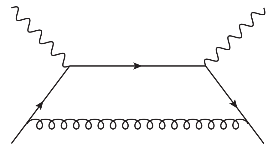
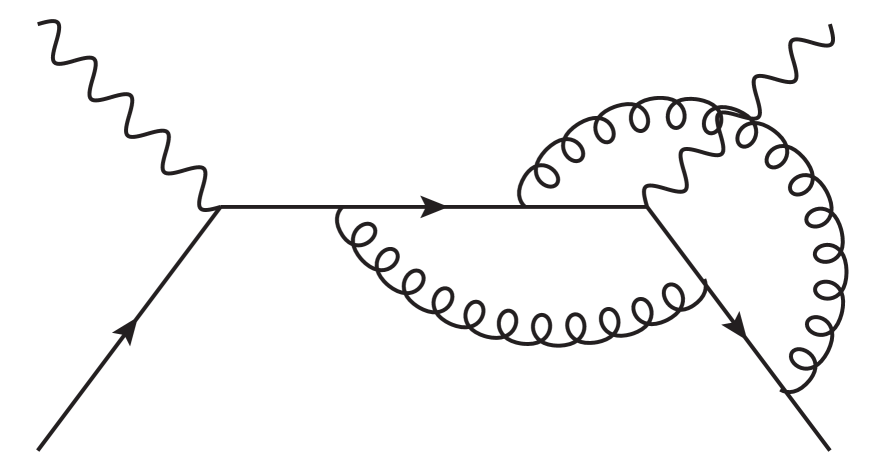
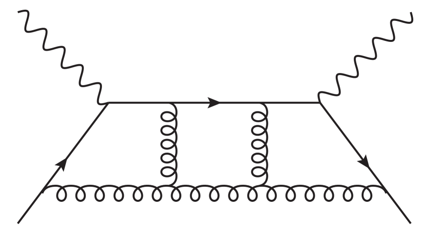
Figure 1: Sample Feynman diagrams for the scattering process of an external current (wavy line) and a heavy quark (solid line). Gluons are represented by curly lines.

Furthermore, for the practical calculation it is convenient to express the non-relativistic quantities $\omega$ and $\vec{v}$ in terms of Lorenz invariants. To this end we introduce

$$y \equiv m_{b}^{2}-s=-\omega\left(2m_{b}\sqrt{1+\vec{v}\,^{2}}+\omega\right)=-m_{b}\,\omega(2+\vec{v}\,^{2})+{O}(\omega^{2},\vec{v}\,^{4})\,,$$ (29)

$$q^{2} \equiv \left[m_{b}\left(\sqrt{1+\vec{v}\,^{2}}-1\right)+\omega\right]^{2}-m_{b}^{2}\vec{v}\,^{2}=-m_{b}\,\vec{v}\,^{2}(m_{b}-\omega)+{O}(\omega^{2},\vec{v}\,^{4})\,.$$ (30)

From these definitions, one can see that we can realize the non-relativistic limits $\lim_{\vec{v}\to 0}$ and $\lim_{m_{b}\to\infty}$ by expanding the amplitude $T$ around the threshold $s=(p+q)^{2}=m_{b}^{2}$ and a subsequent expansion in $q$. In fact, we interpret $\lim_{m_{b}\to\infty}$ as an expansion in the quantity

$$y=m_{b}^{2}-s\leq 0\,,$$ (31)

which we realize with the help of expansion by regions [17, 18]. The expansion $\vec{v}\to 0$, on the other hand, reduces to a naive Taylor expansion in $q$. From the definition of the kinetic mass and the relations in Eqs. (29) and (30) it is clear that we only have to consider terms up to ${O}(y^{-1})$ and ${O}(q^{2})$.

Note that the two limits $\lim_{\vec{v}\to 0}$ and $\lim_{m_{b}\to\infty}$ do not commute. In case we apply first $\lim_{\vec{v}\to 0}$ to $T$ there is no imaginary part.

3 Details of the calculation

In this Section we provide technical details to our calculation and discuss in particular the application of the method of regions [17], the reduction to master integrals and the computation of the latter. We remark that in Ref. [15] no technical details for the calculation to $\mathcal{O}(\alpha_{s}^{2})$ are provided.

3.1 Method of regions

From Eqs. (21) and (22) we know that we have to compute the imaginary part of $T(\omega,\vec{v})$ in the limit $m_{b}\to\infty$, which corresponds to an expansion around $y\to 0$. To this end, we apply the threshold expansion developed in Ref. [17], see also Ref. [18]. Ref. [17] considered the threshold expansion of the heavy quark-photon vertex and identified four different scalings for the loop momenta: hard, soft, potential and ultra-soft. In our case, we only have to consider the threshold of one heavy quark. Thus, the soft and potential regions lead to scaleless integrals, which are set to zero within dimensional regularization. We remain with two regions (hard and ultra-soft) for each loop momentum $k_{i}$ ($i=1,2,3$) with the scalings

hard (h): $$k_{i}\sim m_{b}\,,$$

ultra-soft (us): $$k_{i}\sim y/m_{b}\,,$$ (32)

where $m_{b}$ is the heavy quark mass and $y=m_{b}^{2}-s$ (with $|y|\ll m_{b}^{2}$) measures the distance to the threshold. Note that in our case we have $y<0$. When expanding the denominators we assume that both $p$ and $q$ scale as $m_{b}$.

At one-loop order, there are only two regions. At two loops, we have the regions (uu), (uh) and (hh), and at three loops we have (uuu), (uuh), (uhh) and (hhh). For each diagram, we have cross-checked the scaling of the loop momenta using the program asy [35]. Note that the contributions where all loop momenta are hard can be discarded since there are no imaginary parts. The mixed regions are expected to cancel after renormalization and decoupling of the heavy quark from the running of the strong coupling constant. Nevertheless we performed an explicit calculation of the (uh), (uuh) and (uhh) regions and used the cancellation as cross check. The physical result for the quark mass relation is solely provided by the purely ultra-soft contributions.

A subtlety in connection with the expansion of the denominators arises at two and three loops where either an individual loop momentum or a linear combination of loop momenta can have a definite scaling. Let us call “naive regions” those that can be obtained by assigning a definite scaling to the loop momenta according to Eq. (32), e.g. at two loops (uu) $\equiv k_{1},k_{2}\sim y/m_{b}$, (hu) $\equiv k_{1}\sim m_{b}$ and $k_{2}\sim y/m_{b}$, (hh) $\equiv k_{1},k_{2}\sim m_{b}$.

In case a linear combination of loop momenta flows through a gluon line, it might happen that fewer regions are found than actually exist. No such problem appears with the (heavy) quark lines since they always have a hard component.

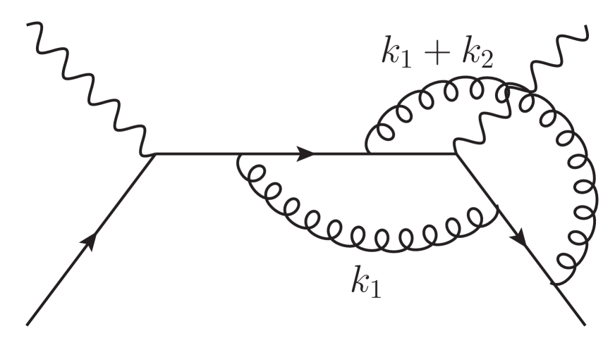
(a)

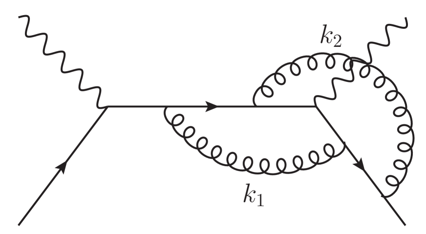
(b)

Figure 2: Two possible momentum routing of a two-loop diagram. The naive regions in the first case (a) do not correspond to all regions while the routing in (b) correctly reveals all regions.

Let us, e.g., consider the two-loop diagram in Fig. 2 and let us assume that $k_{1}+k_{2}$ flows through one of the gluon lines, as shown in Fig. 2(a). If both loop momenta are ultra-soft there is no problem. In case $k_{1}$ is hard and $k_{2}$ is ultra-soft, the gluon line is always hard and there is no imaginary part. Thus one has to consider the case where $k_{1}+k_{2}$ is ultra-soft and both $k_{1}$ and $k_{2}$ are hard. On the contrary, if we consider the momentum routing shown in Fig. 2(b), the gluon line can be ultra-soft $k_{2}\sim y/m_{b}$, while the other gluon can be hard $k_{1}\sim m_{b}$. With this second routing we see that the naive regions cover all possibilities. Therefore for certain choices of momentum routing, the restriction of the scaling to individual loop momenta might miss some of the regions as it ignores potential ultra-soft scaling of linear combinations.

To be sure that we considered all relevant regions, we proceeded as follows: for each diagram we checked that the number of naive regions and the scaling of individual loop momenta according to Eq. (32) agree with those found by asy [35]. If we found fewer regions then we re-routed the loop momenta through the gluon lines, applied the scaling rules and checked again against asy.

As mentioned before, we have to compute the expansions of the individual diagrams up to $\mathcal{O}(y^{-1},q^{2})$. The expansion in $y$ is implemented with the help of expansion by regions and we thus have a definite power counting for the leading behaviour in $y$ for individual terms. However, the Taylor expansion in the momentum $q$ is effectively an expansion in the scalar products

$$q^{2}\quad\text{and}\quad p\cdot q=-\frac{1}{2}\left(y+q^{2}\right)~{}.$$ (33)

In order not to miss terms up to the desired order, we have to expand sufficiently deep in $q$. Since the worst scaling in the ultra-soft region is $\sim y^{-1}$, we have to consider two terms in the $q$ expansion at least. The mixed regions at three-loop order show a behaviour $\sim y^{-3}$. Here we have to consider up to six terms in the $q$ expansion, which leads to high numerator and denominator powers.

3.2 Singlet-type diagrams

Let us in the following discuss the diagrams where one or both external currents couple to a closed massive fermion loop, which is connected to the external heavy quark line via gluons. We refer to these contributions as “singlet-type” diagrams. They occur for the first time at two loops.

The momentum $p$ is always routed through the heavy quark line. As we have seen above, a diagram develops an imaginary part only in those cases where the external heavy quark line is part of a ultra-soft loop and carries the external momentum $p+q$, which leads to a “$-y$” term in the denominator.

(a)

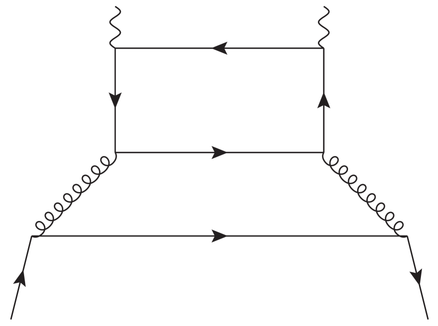
(b)

(c)

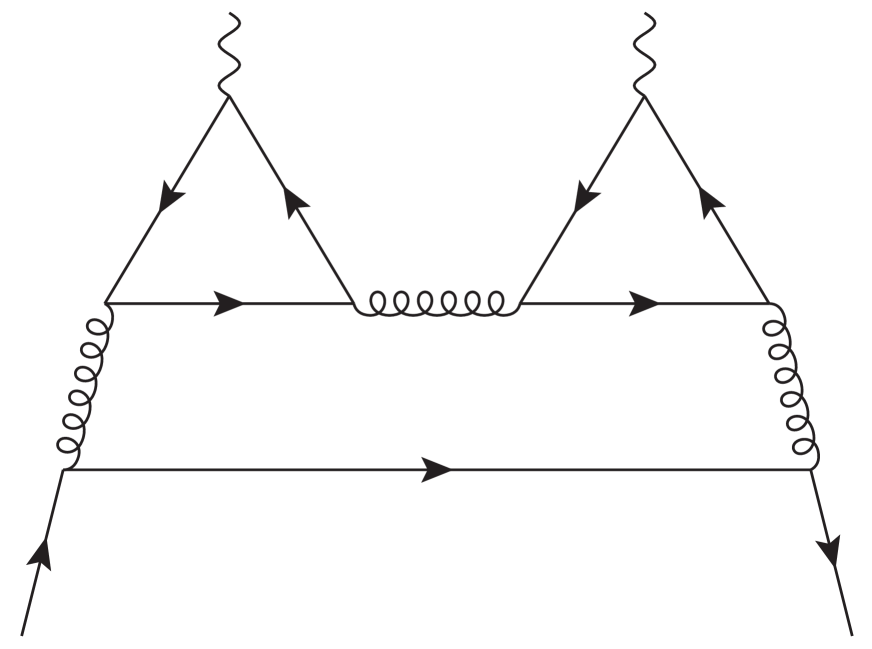
(d)

Figure 3: Sample singlet-type Feynman diagrams. The external currents are drawn with wavy lines, heavy quarks with solid lines and gluons are represented by curly lines. Diagrams (a), (c) and (d) are zero for an external vector current but not for an external scalar current.

At two loops “singlet-type” diagrams appear in two versions:

• One external current couples to a quark triangle which is connected with two gluons to the external heavy quark line (see Fig. 3(a)). The other external current is directly connected to the latter.

  Such contributions have no heavy quark line which is part of a ultra-soft loop and carries the momentum $p+q$. In fact, the application of the method of regions together with the condition that at least one of the loops is ultra-soft, immediately leads to scaleless integrals. For vector currents, such contributions are zero due to Furry’s theorem.

• In a second class of diagrams, the two external currents couple to a quark box which is connected with two gluons to the external heavy quark line (see Fig. 3(b)). Again, no imaginary part can be developed at the threshold $s=m_{b}^{2}$.

At three loops there are the same two classes of Feynman diagrams as at two loops, supplemented by an additional gluon. After applying the same arguments it is easy to see that also here no contribution to the imaginary part of $T(q_{0},\vec{q}\,)$ in Eq. (24) can be constructed, with the exception of diagrams like that one in Fig. 3(c). In these diagrams, one of the currents couples to a quark triangle that is connected to the external heavy quark line with two gluons. An additional gluon couples only to the (external) heavy quark forming the third loop. In that case, the first two loops can be hard and the third loop develops an imaginary part in analogy to the one-loop contribution.

Note that due to Furry’s theorem, these kind of diagrams vanish for external vector currents. However, for the scalar currents they lead to non-zero contributions. We have checked that they cancel against the virtual corrections, which at two-loop order also have contributions from singlet diagrams, see Section 3.4.

There is also a three-loop contribution where both currents are connected to different closed fermion loops (Fig. 3(d)) that are connected to each other and to the external heavy quark line. Here the loop momenta of the closed quark loops are hard, but the third loop momentum can be ultra-soft and in principle produce an imaginary part. However, an explicit calculation shows that these kind of diagrams scale $\sim y^{0}$ and therefore do not enter in the relation for the kinetic mass.

3.3 Vector and scalar currents

As external currents, we use for our calculation both a vector and a scalar current which in coordinate space are given by

$$J^{\mu}_{V} = \bar{b}(x)\gamma^{\mu}b(x)\,,$$

$$J_{S} = m_{b}\,\bar{b}(x)b(x)\,.$$ (34)

In the case of $J_{S}$ we introduce the factor $m$ such that $J_{S}$ has vanishing anomalous dimension. Note that $m$ enters the same renormalization procedure as the mass parameter in the heavy quark propagators.

In spinor space the amplitude $T$ can be written as (ignoring Lorentz indices for an external vector current) $T=p\!\!\!/\,\,\Sigma_{V}+m_{b}\Sigma_{S}$. We multiply by $p\!\!\!/\,\,+m_{b}$ and take the trace. This leads to

$$\mbox{Tr}\left[(p\!\!\!/\,\,+m_{b})T\right] = 4m_{b}^{2}\left(\Sigma_{V}+\Sigma_{S}\right)\,.$$ (35)

In the case of $J_{V}$ the forward scattering amplitude $T$ becomes a tensor of rank 2 and can be parameterized through two structure functions $T_{A}$ and $T_{B}$, which we define as

$$T^{\mu\nu} = T_{A}\left(g^{\mu\nu}-\frac{q^{\mu}q^{\nu}}{q^{2}}\right)+T_{B}\left(\frac{p^{\mu}p^{\nu}}{p\cdot q}-\frac{p^{\mu}q^{\mu}+p^{\nu}q^{\mu}}{q^{2}}+\frac{p\cdot q}{q^{2}}g^{\mu\nu}\right)\,.$$ (36)

We have used the symmetry of the forward scattering amplitude $T^{\mu\nu}=T^{\nu\mu}$ and the transversity $q_{\mu}T^{\mu\nu}=q_{\nu}T^{\mu\nu}=0$.

One can construct projectors on $T_{A}$ and $T_{B}$ which can be written as linear combinations of the two structures

$$P_{1}^{\mu\nu} = \frac{p^{\mu}p^{\nu}}{m_{b}^{2}}\,,$$ (37)

$$P_{2}^{\mu\nu} = g^{\mu\nu}\,.$$ (38)

We find

$$(d-2)P_{A}^{\mu\nu} = \frac{m_{b}^{2}q^{2}}{m_{b}^{2}q^{2}-(p\cdot q)^{2}}P_{2}^{\mu\nu}-\frac{m_{b}^{2}q^{2}\left((d-2)(p\cdot q)^{2}+m_{b}^{2}q^{2}\right)}{\left((p\cdot q)^{2}-m_{b}^{2}q^{2}\right)^{2}}P_{1}^{\mu\nu}$$ (39)

$$\stackrel{{\scriptstyle q^{2}\to 0}}{{\longrightarrow}} P_{2}^{\mu\nu}-P_{1}^{\mu\nu}+\frac{y}{2m_{b}^{2}}\left(P_{2}^{\mu\nu}-dP_{1}^{\mu\nu}\right)\,,$$

$$(d-2)P_{B}^{\mu\nu} = \frac{(d-1)m_{b}^{2}p\cdot q(q^{2})^{2}}{\left((p\cdot q)^{2}-m_{b}^{2}q^{2}\right)^{2}}P_{1}^{\mu\nu}+\frac{p\cdot qq^{2}}{p\cdot q^{2}-m_{b}^{2}q^{2}}P_{2}^{\mu\nu}$$ (40)

$$\stackrel{{\scriptstyle q^{2}\to 0}}{{\longrightarrow}} \frac{2y}{m_{b}^{2}}\left(P_{2}^{\mu\nu}-(d-1)P_{1}^{\mu\nu}\right)\,.$$

For both projectors the limits for $y\to 0$ and $q^{2}\to 0$ exist. Thus, in practice we can simply apply $P_{1}^{\mu\nu}$ and $P_{2}^{\mu\nu}$ and construct the physical structure functions afterwards by considering the proper linear combinations. It is interesting to note that $P_{1}^{\mu\nu}$ and $P_{2}^{\mu\nu}$ applied to $T^{\mu\nu}$ lead to a scaling $\sim 1/y$. For this reason the term $P_{2}^{\mu\nu}-P_{1}^{\mu\nu}$ in Eq. (39) has to vanish and both $P_{A}^{\mu\nu}$ and $P_{B}^{\mu\nu}$ (considered as linear combinations of $P_{1}^{\mu\nu}$ and $P_{2}^{\mu\nu}$) have to scale $\sim y$ in the limit $q^{2}\to 0$. As a consequence, we can apply either $P_{1}^{\mu\nu}$ or $P_{2}^{\mu\nu}$ to compute the kinetic mass. The difference to the application of proper linear combinations (i.e. $P_{A}$ and $P_{B}$) is a $d$- and $m$-dependent prefactor which drops out in the definition of the quantities $\overline{\Lambda}(\mu)$ and $\mu_{\pi}^{2}(\mu)$ from Eq. (22).

3.4 Virtual corrections

Virtual corrections enter the denominator of Eq. (28). For the two- and three-loop kinetic mass we need one- and two-loop virtual corrections, respectively. Furthermore, we only need the static limit ($q^{2}=0$), which can be obtained, e.g., from [36, 37]. Note that in this limit the form factors are infrared finite (as are the real radiation corrections which we compute).

For the case of the vector current the effective vertex $\Gamma^{V}_{\mu}$ can be expressed in terms of two form factors contributing to the virtual corrections

$$\Gamma^{V}_{\mu} = -i\left(F_{1}\gamma_{\mu}+F_{2}\frac{i}{2m_{b}}\sigma_{\mu\nu}q^{\nu}\right),$$ (41)

with $\sigma_{\mu\nu}=\frac{i}{2}\left[\gamma_{\mu},\gamma_{\nu}\right]$. After inserting $\Gamma^{V}_{\mu}$ into the tree level expression, we see that the contribution of the virtual corrections is given by

$$V_{i} = \delta(y)\text{Tr}\left[(\not{p}+m_{b}){\Gamma^{V}_{\mu}}^{*}(\not{p}+\not{q}+m_{b})\Gamma^{V}_{\nu}\right]P_{i}^{\mu\nu},$$ (42)

with $P_{1}^{\mu\nu}=p^{\mu}p^{\nu}/m_{b}^{2}$ and $P_{2}^{\mu\nu}=g_{\mu\nu}$. The delta function $\delta(y)$ ensures that we have $s=m_{b}^{2}$. We find

$$V_{1} = \delta(y)\left[-2\left|F_{1}\right|^{2}\left(q^{2}-4m_{b}^{2}\right)+\left|F_{2}\right|^{2}\frac{q^{4}}{8m_{b}^{4}}\left(q^{2}-4m_{b}^{2}\right)\right]\,,$$

$$V_{2} = \delta(y)\left[\left|F_{1}\right|^{2}\left(2(d-2)q^{2}+8m_{b}^{2}\right)+\left|F_{2}\right|^{2}\frac{q^{2}}{2}\left(8-4d-\frac{q^{2}}{m_{b}^{2}}\right)\right]\,.$$ (43)

From the definition of the kinematic mass we see that virtual corrections always multiply lower-order real emissions (which vanish for $q^{2}\to 0$). Therefore only the non-vanishing parts of Eq. (43) in the limit $q^{2}\to 0$ contribute, which is proportional to $|F_{1}|^{2}$. Note, however, that $F_{1}$ has a vanishing static limit to all orders in perturbation theory $F_{1}(q^{2}=0)=0$ and thus the kinetic mass does not receive contributions from virtual corrections in the case of an external vector current.

This is different for the scalar current. We define

$$\Gamma^{S} = -iF_{S}\,.$$ (44)

which leads to

$$V_{S} = \delta(y)\left|F_{S}\right|^{2}\left[8m_{b}^{2}-2q^{2}\right]\,.$$ (45)

Since $F_{S}(q^{2}=0)\neq 0$ we are left with a non-vanishing contribution. For the three-loop correction to the $m^{\rm kin}$–$m^{\rm OS}$ relation we need $F_{S}(q^{2}=0)$ up to two loops which is given by (see, e.g., Refs. [36, 37])

$$F_{S}(0) = \frac{\alpha_{s}}{4\pi}C_{F}\left(-2+3l_{m}\right)+\left(\frac{\alpha_{s}}{4\pi}\right)^{2}C_{F}\biggl{\{}C_{A}\biggl{[}-6\zeta_{3}+\frac{11l_{m}^{2}}{2}+\frac{53l_{m}}{6}+\pi^{2}\left(4l_{2}-\frac{4}{3}\right)$$ (46)

$$-\frac{123}{8}\biggr{]}+C_{F}\left[12\zeta_{3}+\frac{9l_{m}^{2}}{2}-\frac{9l_{m}}{2}+\pi^{2}\left(5-8l_{2}\right)+\frac{193}{8}\right]$$

$$+T_{F}\left[n_{h}\left(-2l_{m}^{2}-\frac{2l_{m}}{3}-\frac{8\pi^{2}}{3}+\frac{51}{2}\right)+n_{l}\left(-2l_{m}^{2}-\frac{2l_{m}}{3}-\frac{4\pi^{2}}{3}+\frac{11}{2}\right)\right]$$

$$+T_{F}n_{h}\left(\frac{16\pi^{2}}{3}-32\right)\biggr{\}}\,,$$

with $l_{m}=\ln(\mu_{s}^{2}/m_{b}^{2})$ and $l_{2}=\ln(2)$. $C_{A}=N_{C}$ and $C_{F}=(N_{C}^{2}-1)/(2N_{C})$ are SU($N_{C}$) colour factors, $T_{F}=1/2$, $n_{l}$ is the number of massless quarks and $n_{h}=1$ is introduced for convenience for closed loops of fermions with mass $m_{b}$. The last term in Eq. (46) corresponds to the contributions from singlet-type diagrams. Note that our final result does not depend on the renormalization scheme used for the external currents. In fact, the vector current does not get renormalized and in the case of the scalar current we renormalize the mass parameter $m_{b}$ introduced in Eq. (34) in the $\overline{\mathrm{MS}}$ scheme.

3.5 Partial fraction decomposition

The starting point of our calculation are four-point functions with forward-scattering kinematics. After we Taylor-expand in $q$, we remain with only one external momentum, which is present in the denominators. Thus, at most 2, 5 and 9 denominators can be linear independent at one, two and three loops, respectively. On the other hand, general four-point functions contain up to 4, 7 and 10 lines and thus, in general, a partial fraction decomposition is required, which decomposes products of linear dependent propagators into terms with only linear independent factors.

At one- and two-loop order, it is straightforward to implement the partial fraction decomposition manually. However, at three loops many different cases appear and an automation of the procedure is recommended. In our calculation we use the program LIMIT developed by Florian Herren [38, 39]. The program is written in Mathematica and internally uses LiteRed [40]. Let us briefly summarize its mode of operation.

We start by grouping diagrams according to their denominator structure into preliminary families, which we supplement with irreducible numerators in order to have complete families. This is a necessary step for the reduction to master integrals which is performed at a later stage. Note that some of the denominators can still be linearly dependent. Furthermore, at this step we do not apply any symmetry transformation to minimize the number of different families. The goal of the program is to find all relations due to partial fraction decomposition. Afterwards the resulting set of families is minimized.

In the first part the program goes through the list of denominators of each family, selects those that are linearly dependent and produces replacement rules that allow for partial fraction decomposition after their iterative application. This step has to be applied recursively to ensure that all denominators are linearly independent. Note that partial fraction decomposition increases the number of families. In our application we start at two loops with {48,16} in the {(uu),(uh)} regions and we end up with {90,23} families with linearly independent denominators. At three loops, we have {510,339,314} families in the {(uuu),(uuh),(uhh)} regions which result in {2650,906,531} families after partial fraction decomposition.

Many of the resulting families are equivalent and can be mapped onto each other. The second part of the program finds these relations and provides rules to map the scalar integrals into a minimal set of families. The program relies on LiteRed to find these rules. In general the program has to find two types of mappings. The first type corresponds to mappings between families that differ only by their momentum routing. These mappings are obtained by computing the $U$ and $F$ polynomials for all families and using the LiteRed command FindExtSymmetries[] to map all families with the same polynomials to a representative one. The second type corresponds to mappings of families with a larger number of numerators onto families with fewer numerators but more denominators. All replacement rules can be exported to FORM [41] statements.

In total we find {2,2} families in the {(uu),(uh)} regions at two loops and at three-loop order {14,4,3} in the {(uuu),(uuh),(uhh)} regions, respectively. Their definitions are given in the next subsection.

3.6 Integral families and reduction to MIs

After partial fraction decomposition and mapping of equivalent families to each other, we are left with only a small number of families. In general they have a number of irreducible numerators which are either formed by the scalar product of the loop momenta with the external momenta $k_{i}\cdot q$, $k_{i}\cdot p$ or scalar products of loop momenta $k_{i}\cdot k_{j}$. They appear in particular in those cases where both hard and ultra-soft regions are present since the integrals factorize. In principle one can apply a tensor decomposition to get rid of such scalar products. However, we chose to include them into the definition of the integral families. Thus, also for the cases where the (two- and three-loop) integrations factorize we pass the corresponding scalar functions to the reduction programs LiteRed [40] and Fire [42], which means that effectively the tensor reduction is performed by these programs. Note that in such cases all master integrals factorize into a hard and ultra-soft part.

Since the expansions in the mixed regions have to be quite deep in order to calculate the diagrams up to $\mathcal{O}(y^{-1},q^{2})$, the indices of the scalar integrals become large. In the mixed regions, we had to reduce about $10^{6}$ integrals with the absolute value of the indices reaching up to 12. In the ultra-soft region, we only had to reduce about $10^{5}$ scalar integrals with indices reaching up to 6. Nevertheless, reducing these integrals using either LiteRed or Fire took roughly two days. We observed that in particular in the mixed regions LiteRed performed better in those cases where high numerator and denominator powers had to be reduced.

In the following we provide the definition of the integral families up to three loops where the factors after the semi-colon correspond to numerators. We do not show the “$-i0$” prescription which is present in all denominator factors. At two- and three-loop order we have both the pure-ultra-soft and the mixed hard-ultra-soft regions.

At one-loop order we only have one family which is given by

fam1lu:	$-k_{1}^{2},-2k_{1}\cdot p+y;$	$-k_{1}\cdot q$

At two loops we have two families in the (uu)-region:

fam2luu1:	$-k_{1}^{2},-(k_{1}-k_{2})^{2},-k_{2}^{2},-2p\cdot k_{1}+y,-2p\cdot k_{2}+y;$	$-q\cdot k_{1},-q\cdot k_{2}$;
fam2luu2:	$-k_{1}^{2},-(k_{1}-k_{2})^{2},-k_{2}^{2},-2p\cdot k_{1}+y,-2p\cdot k_{2};$	$-q\cdot k_{1},-q\cdot k_{2};$

and one family in the uh-region:

fam2luh1:	$-k_{1}^{2},-k_{2}^{2},-(k_{2}+p)^{2}+m_{b}^{2},-2p\cdot k_{1}+y;$	$-k_{1}\cdot k_{2},-k_{1}\cdot q,-k_{2}\cdot q$.

Here also the scalar product $k_{1}\cdot k_{2}$ is an irreducible numerator. For the calculation with a massive charm quark (see Section 4) we have in addition the following family:

fam2luh2:	$-k_{1}^{2},-k_{2}^{2}+m_{c}^{2},-2p\cdot k_{1}+y;$	$-k_{1}\cdot k_{2},-k_{2}\cdot p,-k_{1}\cdot q,-k_{2}\cdot q$.

At three loops we have 14 families in the (uuu), two in the (uuh) and two in the (uhh) regions for the calculation with a massless charm quark. A massive charm quark requires two and one additional families in the (uuh) and (uhh) regions, respectively. All definitions are given in Tab. 1.

fam3luuu1:	$-k_{1}^{2},-k_{2}^{2},-k_{3}^{2},-(k_{1}-k_{3})^{2},-(k_{2}-k_{3})^{2},-2p\cdot k_{1}+y,-2p\cdot k_{2}+y,-2p\cdot k_{3}+y;$
	$-k_{1}\cdot k_{2},-q\cdot k_{1},-q\cdot k_{2},-q\cdot k_{3}$
fam3luuu2:	$-k_{1}^{2},-k_{2}^{2},-(k_{1}-k_{2})^{2},-(k_{1}-k_{3})^{2},-(k_{2}-k_{3})^{2},-2p\cdot k_{1}+y,-2p\cdot k_{2}+y,-2p\cdot k_{3}+y;$
	$-k_{3}^{2},-q\cdot k_{1},-q\cdot k_{2},-q\cdot k_{3}$
fam3luuu3:	$-k_{1}^{2},-k_{2}^{2},-k_{3}^{2},-(k_{1}-k_{2})^{2},-(k_{1}-k_{3})^{2},-(k_{2}-k_{3})^{2},-2p\cdot k_{1}+y,-2p\cdot k_{2}+y;$
	$-p\cdot k_{3},-q\cdot k_{1},-q\cdot k_{2},-q\cdot k_{3}$
fam3luuu4:	$-2p\cdot k_{2},-k_{2}^{2},-(k_{1}-k_{2})^{2},-k_{3}^{2},-(k_{1}-k_{3})^{2},-(k_{1}-k_{2}-k_{3})^{2},-2p\cdot k_{1}+y,-2p\cdot k_{3}+y;$
	$-k_{1}^{2},-q\cdot k_{1},-q\cdot k_{2},-q\cdot k_{3}$
fam3luuu5:	$-2p\cdot k_{1},-2p\cdot k_{2},-k_{2}^{2},-(k_{1}-k_{2})^{2},-k_{3}^{2},-(k_{1}-k_{3})^{2},-(k_{1}-k_{2}-k_{3})^{2},-2p\cdot k_{3}+y;$
	$-k_{1}^{2},-q\cdot k_{1},-q\cdot k_{2},-q\cdot k_{3}$
fam3luuu6:	$-k_{1}^{2},-2p\cdot k_{2},-k_{2}^{2},-(k_{1}-k_{2})^{2},-k_{3}^{2},-(k_{1}-k_{3})^{2},-2p\cdot k_{1}+y,-2p\cdot k_{3}+y;$
	$-k_{2}\cdot k_{3},-q\cdot k_{1},-q\cdot k_{2},-q\cdot k_{3}$
fam3luuu7:	$-2p\cdot k_{1},-k_{1}^{2},-2p\cdot k_{2},-k_{2}^{2},-(k_{1}-k_{2})^{2},-k_{3}^{2},-(k_{1}-k_{3})^{2},-2p\cdot k_{3}+y;$
	$-k_{2}\cdot k_{3},-q\cdot k_{1},-q\cdot k_{2},-q\cdot k_{3}$
fam3luuu8:	$-2p\cdot k_{1},-k_{1}^{2},-(k_{1}-k_{2})^{2},-k_{3}^{2},-(k_{1}-k_{3})^{2},-(k_{2}-k_{3})^{2},-2p\cdot k_{2}+y,-2p\cdot k_{3}+y;$
	$-k_{2}^{2},-q\cdot k_{1},-q\cdot k_{2},-q\cdot k_{3}$
fam3luuu9:	$-2p\cdot k_{1},-k_{1}^{2},-2p\cdot k_{2},-(k_{1}-k_{2})^{2},-k_{3}^{2},-(k_{1}-k_{3})^{2},-(k_{2}-k_{3})^{2},-2p\cdot k_{3}+y;$
	$-k_{2}^{2},-q\cdot k_{1},-q\cdot k_{2},-q\cdot k_{3}$
fam3luuu10:	$-k_{1}^{2},-2p\cdot k_{2},-k_{2}^{2},-(k_{1}-k_{2})^{2},-k_{3}^{2},-(k_{1}+k_{3})^{2},-(k_{2}+k_{3})^{2},-2p\cdot k_{1}+y;$
	$-p\cdot k_{3},-q\cdot k_{1},-q\cdot k_{2},-q\cdot k_{3}$
fam3luuu11:	$-2p\cdot k_{1},-k_{1}^{2},-k_{2}^{2},-(k_{1}-k_{2})^{2},-2p\cdot k_{3},-k_{3}^{2},-(k_{2}-k_{3})^{2},-2p\cdot k_{2}+y;$
	$-k_{1}\cdot k_{3},-q\cdot k_{1},-q\cdot k_{2},-q\cdot k_{3}$
fam3luuu12:	$-2p\cdot k_{1},-k_{1}^{2},-2p\cdot k_{2},-k_{2}^{2},-(k_{1}-k_{2})^{2},-(k_{1}-k_{3})^{2},-(k_{2}-k_{3})^{2},-2p\cdot k_{3}+y;$
	$-k_{3}^{2},-q\cdot k_{1},-q\cdot k_{2},-q\cdot k_{3}$
fam3luuu13:	$-k_{1}^{2},-k_{2}^{2},-(k_{1}-k_{3})^{2},-(k_{2}-k_{3})^{2},-(k_{1}+k_{2}-k_{3})^{2},-2p\cdot k_{1}+y,-2p\cdot k_{2}+y,-2p\cdot k_{3}+y;$
	$-k_{3}^{2},-q\cdot k_{1},-q\cdot k_{2},-q\cdot k_{3}$
fam3luuu14:	$-2p\cdot k_{1},-k_{1}^{2},-2p\cdot k_{2},-k_{2}^{2},-(k_{1}-k_{3})^{2},-(k_{2}-k_{3})^{2},-(k_{1}+k_{2}-k_{3})^{2},-2p\cdot k_{3}+y;$
	$-k_{3}^{2},-q\cdot k_{1},-q\cdot k_{2},-q\cdot k_{3}$
fam3luuh1:	$-k_{1}^{2},-k_{2}^{2},-(k_{1}-k_{2})^{2},-k_{3}^{2},-(k_{3}+p)^{2}-m_{b}^{2},-2p\cdot k_{1}+y,-2p\cdot k_{2}+y;$
	$-k_{1}\cdot k_{3},-k_{2}\cdot k_{3},-q\cdot k_{1},-q\cdot k_{2},-q\cdot k_{3}$
fam3luuh2:	$-k_{1}^{2},-k_{2}^{2},-2p\cdot k_{1}+2p\cdot k_{2},-(k_{1}+k_{2})^{2},-k_{3}^{2},-(k_{3}+p)^{2}-m_{b}^{2},-2p\cdot k_{2}+y;$
	$-k_{1}\cdot k_{3},-k_{2}\cdot k_{3},-q\cdot k_{1},-q\cdot k_{2},-q\cdot k_{3}$
fam3luuh3:	$-k_{1}^{2},-k_{2}^{2},-(k_{1}-k_{2})^{2},-k_{3}^{2}+m_{c}^{2},-2p\cdot k_{1}+y,-2p\cdot k_{2}+y;$
	$-k_{1}\cdot k_{3},-k_{2}\cdot k_{3},-p\cdot k_{3},-q\cdot k_{1},-q\cdot k_{2},-q\cdot k_{3}$
fam3luuh4:	$-k_{1}^{2},-k_{2}^{2},-(k_{1}-k_{2})^{2},-k_{3}^{2}+m_{c}^{2},-2p\cdot k_{1}+y,-2p\cdot k_{2};$
	$-k_{1}\cdot k_{3},-k_{2}\cdot k_{3},-p\cdot k_{3},-q\cdot k_{1},-q\cdot k_{2},-q\cdot k_{3}$
fam3luhh1:	$-k_{1}^{2},-k_{2}^{2},-2p\cdot k_{2}+k_{2}^{2},-k_{3}^{2},-2p\cdot k_{3}+k_{3}^{2},-2p\cdot k_{2}+2p\cdot k_{3}+k_{2}^{2}+2k_{2}\cdot k_{3}+k_{3}^{2},-2p\cdot k_{1}+y;$
	$-k_{1}\cdot k_{2},-k_{1}\cdot k_{3},-q\cdot k_{1},-q\cdot k_{2},-q\cdot k_{3}$
fam3luhh2:	$-k_{1}^{2},-k_{2}^{2},-2p\cdot k_{2}+k_{2}^{2},-k_{3}^{2},-2p\cdot k_{3}+k_{3}^{2},-k_{2}^{2}-2k_{2}\cdot k_{3}+k_{3}^{2},-2p\cdot k_{1}+y;$
	$-k_{1}\cdot k_{2},-k_{1}\cdot k_{3},-q\cdot k_{1},-q\cdot k_{2},-q\cdot k_{3}$
fam3luhh3:	$-k_{1}^{2},-k_{2}^{2},-2p\cdot k_{2}+k_{2}^{2},-k_{3}^{2}+m_{c}^{2},-(k_{2}-k_{3})^{2}+m_{c}^{2},-2p\cdot k_{1}+y;$
	$-k_{1}\cdot k_{2},-k_{1}\cdot k_{3},-p\cdot k_{3},-q\cdot k_{1},-q\cdot k_{2},-q\cdot k_{3}$

Table 1: Three-loop integral families in the (uuu), (uuh) and (uhh) regions. The factors after the semi-colon correspond to numerators.

3.7 Master integrals

After reduction to master integrals and their subsequent minimization across all families, the amplitude can be expressed in terms of 1, 3 and 20 ultra-soft master integrals at one-, two- and three-loop order, respectively. Many of them can be computed introducing Feynman parameters and integrating step-by-step, even for general dimension $d=4-2\epsilon$. In the following we denote them by the letter $I$. Master integrals in the mixed regions are denoted by the letters $J$ and $K$.

At one- and two-loop order the results for the master integrals are given by

$$I^{1l} = Ny^{d-3}(m_{b}^{2})^{1-d/2}\Gamma(d/2-1)\Gamma(3-d)\,,$$

$$J^{1l} = \int\frac{{\rm d}^{d}k_{1}}{(2\pi)^{d}}\frac{1}{-k_{1}^{2}+m_{b}^{2}}=N(m_{b}^{2})^{d/2-1}\Gamma(1-d/2)\,,$$ (47)

and

$$I_{1}^{2l} = \left(I^{1l}\right)^{2}=N^{2}y^{2d-6}(m_{b}^{2})^{2-d}\Gamma^{2}\left(\tfrac{d}{2}-1\right)\Gamma^{2}\left(3-d\right),$$

$$I_{2}^{2l} = N^{2}y^{2d-6}(m_{b}^{2})^{2-d}\Gamma^{2}\left(\tfrac{d}{2}-1\right)\Gamma\left(3-d\right)\frac{\Gamma(2d-5)\Gamma(6-2d)}{\Gamma(d-2)}\,,$$

$$I_{3}^{2l} = N^{2}y^{2d-5}(m_{b}^{2})^{2-d}\Gamma^{2}\left(\tfrac{d}{2}-1\right)\Gamma(5-2d)\,,$$

$$J_{1}^{2l} = I^{1l}J^{1l}=N^{2}y^{d-3}\Gamma\left(1-\tfrac{d}{2}\right)\Gamma\left(\tfrac{d}{2}-1\right)\Gamma(3-d)\,,$$ (48)

with

$$N = \frac{i}{(4\pi)^{d/2}}\,.$$ (49)

Note that the last integral originates from the (uh) region and factorizes into a massive tadpole integral and the one-loop ultra-soft master integral. Graphical representation of the ultra-soft one- and two-loop master integrals can be found in Fig. 4.

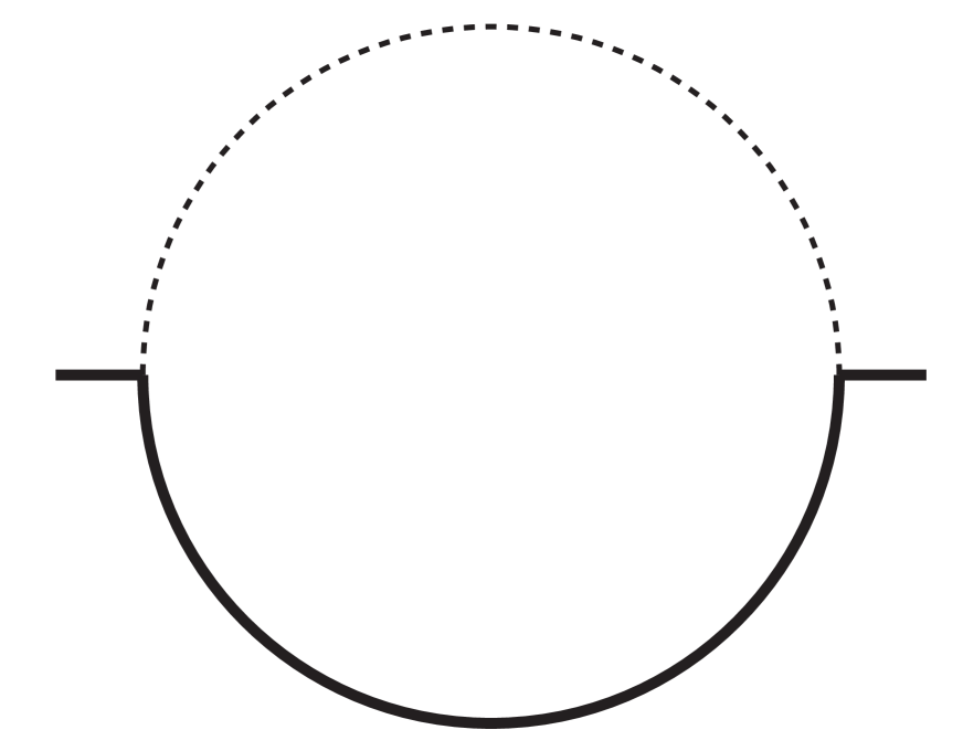
$I^{1l}$

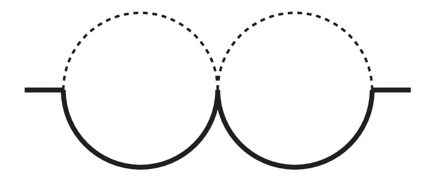
$I^{2l}_{1}$

$I^{2l}_{2}$

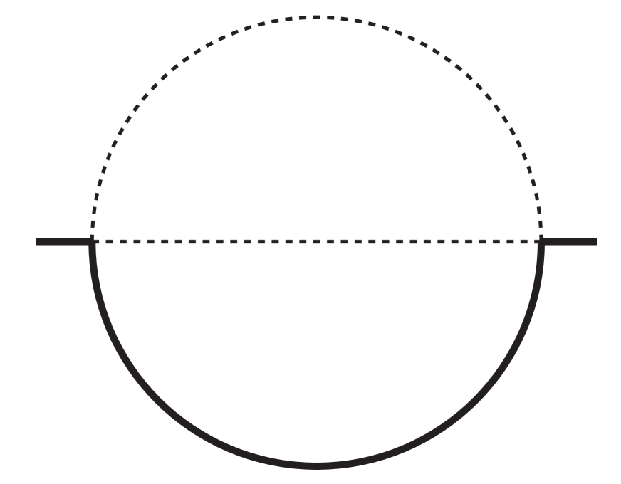
$I^{2l}_{3}$

Figure 4: The one- and two-loop master integrals for the double ultra-soft region. Dashed lines represent massless propagators, while solid lines and double lines represent the linear massive ($2p\cdot k_{i}-y$) and massless ($2p\cdot k_{i}$) HQET-like propagators, respectively, with $p^{2}=m_{b}^{2}$ and the loop momentum $k_{i}$ ($i=1,2$).

Also at three loops, eleven (out of 20) master integrals can be expressed in term of $\Gamma$ functions and are thus available to all orders in $\epsilon$. They are given by

$$I_{1}^{3l} =N^{3}y^{3d-7}(m_{b}^{2})^{3-3d/2}\,\Gamma^{3}(d/2-1)\Gamma(7-3d),$$

$$I_{2}^{3l} =N^{3}y^{3d-8}(m_{b}^{2})^{3-3d/2}\,\frac{\Gamma^{3}(d/2-1)\Gamma^{2}(3-d)\Gamma(8-3d)}{\Gamma(6-2d)},$$

$$I_{3}^{3l} =N^{3}y^{3d-8}(m_{b}^{2})^{3-3d/2}\,\Gamma^{3}(d/2-1)\Gamma(3-d)\Gamma(5-2d),$$

$$I_{4}^{3l} =N^{3}y^{3d-9}(m_{b}^{2})^{4-3d/2}\,\frac{\Gamma^{4}(d/2-1)\Gamma^{2}(2-d/2)\Gamma(3d/2-4)\Gamma(9-3d)}{\Gamma^{2}(d-2)\Gamma(4-d)},$$

$$I_{6}^{3l} =N^{3}y^{3d-9}(m_{b}^{2})^{3-3d/2}\,\Gamma^{3}(d/2-1)\Gamma^{3}(3-d),$$

$$I_{8}^{3l} =N^{3}y^{3d-8}(m_{b}^{2})^{3-3d/2}\,\frac{\Gamma^{3}(d/2-1)\Gamma(3-d)\Gamma(2d-5)\Gamma(8-3d)}{\Gamma(d-2)},$$

$$I_{9}^{3l} =N^{3}y^{3d-8}(m_{b}^{2})^{3-3d/2}\,\frac{\Gamma^{3}(d/2-1)\Gamma(5-2d)\Gamma(3d-7)\Gamma(8-3d)}{\Gamma(d-2)},$$

$$I_{10}^{3l} =N^{3}y^{3d-8}(m_{b}^{2})^{3-3d/2}\,\frac{\Gamma^{3}(d/2-1)\Gamma(3-d)\Gamma(3d-7)\Gamma(8-3d)}{\Gamma(2d-4)},$$

$$I_{13}^{3l} =N^{3}y^{3d-9}(m_{b}^{2})^{3-3d/2}\,\frac{\Gamma^{3}(d/2-1)\Gamma(3-d)\Gamma(2d-5)\Gamma(6-2d)\Gamma(3d-8)\Gamma(9-3d)}{\Gamma^{2}(d-2)},$$

$$I_{15}^{3l} =N^{3}y^{3d-9}(m_{b}^{2})^{3-3d/2}\,\frac{\Gamma^{3}(d/2-1)\Gamma^{2}(3-d)\Gamma(2d-5)\Gamma(6-2d)}{\Gamma(d-2)},$$

$$I_{17}^{3l} =N^{3}y^{3d-9}(m_{b}^{2})^{3-3d/2}\,\frac{\Gamma^{3}(d/2-1)\Gamma^{2}(3-d)\Gamma(3d-8)\Gamma(9-3d)}{\Gamma(d-2)}\,,$$ (50)

where the corresponding integral representation is easily obtained from the pictures shown in Fig. 5. In Appendix C, we provide auxiliary integrals useful to obtain the results in Eq. (50).

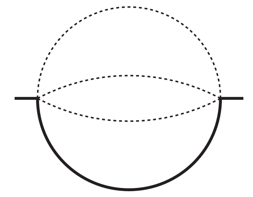
$I^{3l}_{1}$

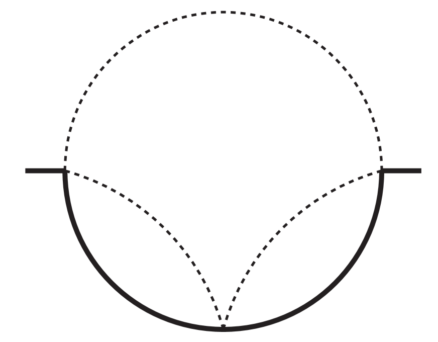
$I^{3l}_{2}$

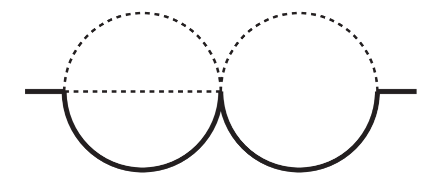
$I^{3l}_{3}$

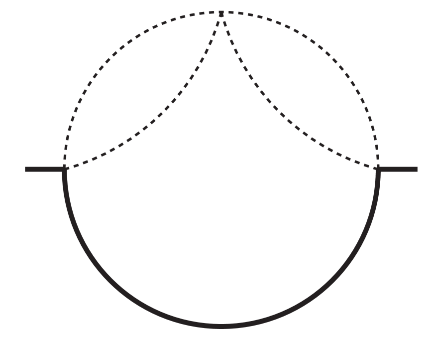
$I^{3l}_{4}$

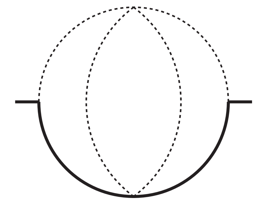
$I^{3l}_{5}$

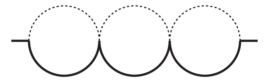
$I^{3l}_{6}$

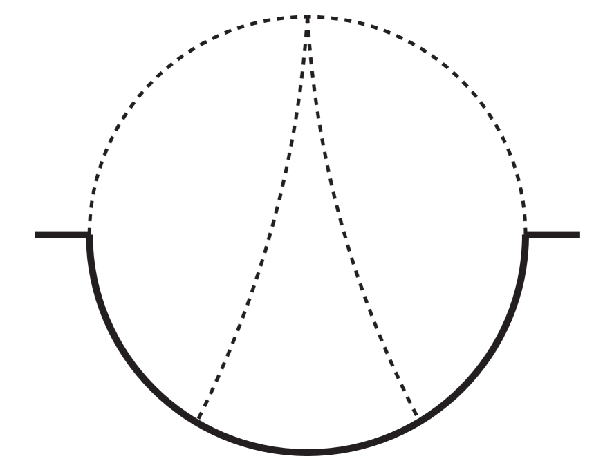
$I^{3l}_{7}$

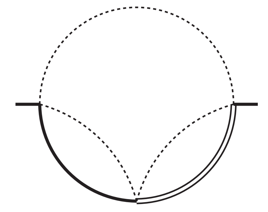
$I^{3l}_{8}$

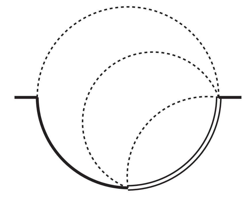
$I^{3l}_{9}$

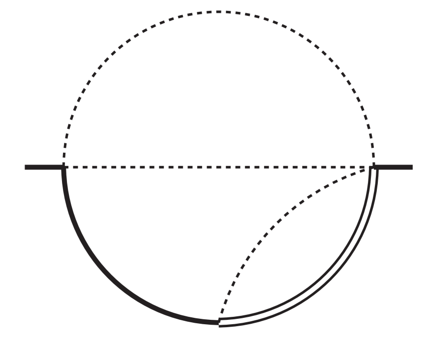
$I^{3l}_{10}$

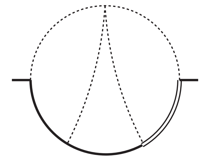
$I^{3l}_{11}$

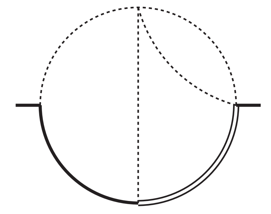
$I^{3l}_{12}$

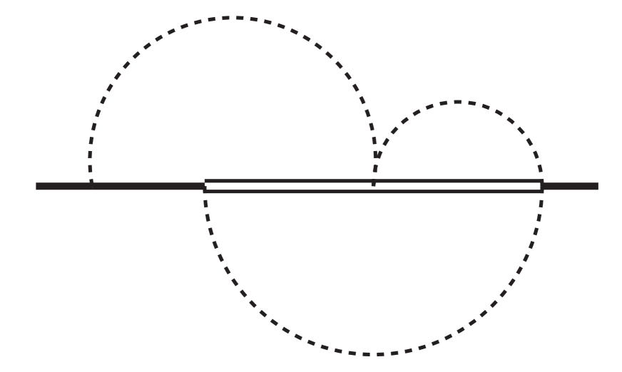
$I^{3l}_{13}$

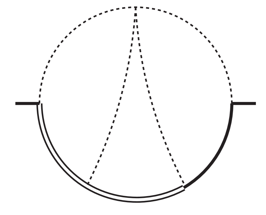
$I^{3l}_{14}$

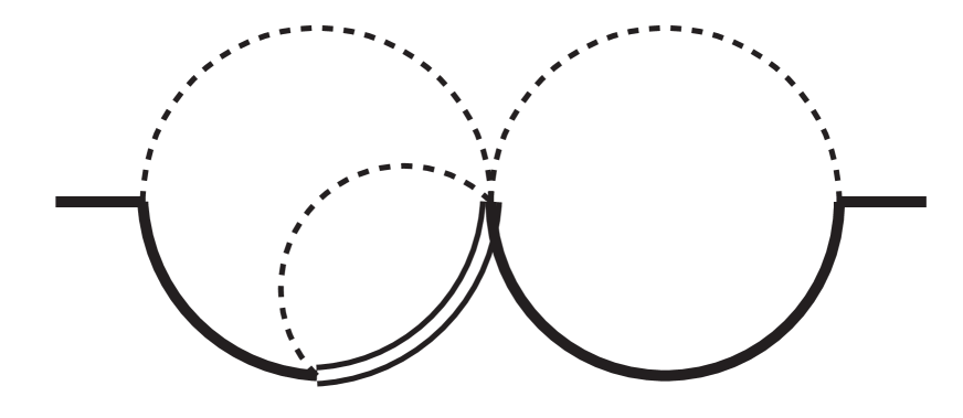
$I^{3l}_{15}$

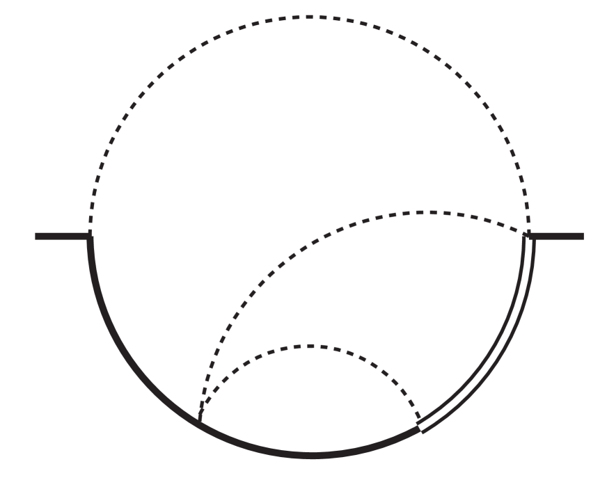
$I^{3l}_{16}$

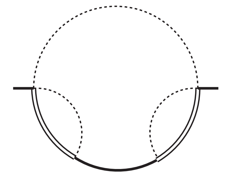
$I^{3l}_{17}$

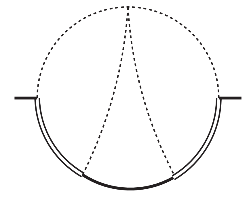
$I^{3l}_{18}$

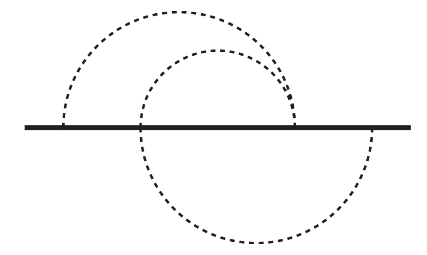
$I^{3l}_{19}$

$I^{3l}_{20}$

Figure 5: The three-loop master integrals for the triple ultra-soft region. The same notation as in Fig. 4 is used.

For the remaining nine integrals in the (uuu) region, we obtained analytic results for the $\epsilon$ expansion with the help of the Mellin-Barnes method [18]. We managed to derive up to four-dimensional representations. In the case of one- and two-dimensional Mellin-Barnes representations (which applies to 7 master integrals) we computed the $\epsilon$ expansion by closing the integration contour and summing up the residues analytically with the packages Sigma [43], EvaluateMultiSums [44] together with HarmonicSums [45]. For the analytic manipulation of the Mellin-Barnes integrals, the program package MB [46, 47] was very useful. Additionally, we managed to obtain high-precision numerical results and use the PSLQ [48] algorithm to reconstruct the analytic expressions. To obtain these results for higher dimensional integrals, the program mpmath [49] was used. All of our analytic expressions were cross-checked using the program FIESTA [50].

For the master integral $I_{11}^{3l}$, we obtained initially a threefold Mellin-Barnes representation, which could be reduced to a twofold representation by applying Barnes-Lemmas after the $\epsilon$-expansion. Then we proceeded as described above.

The only master integral we were not able to determine with Mellin-Barnes methods to the necessary order in $\epsilon$ was $I_{7}^{3l}$. We mention that we calculate $I_{7}^{3l}$ up to transcendental weight 5, i.e. one order higher then needed for the current calculation. The higher order terms are necessary for the calculation in [51]. For the calculation of $I_{7}^{3l}$ it was necessary to apply a different strategy. For this integral, we introduced a second mass scale $x$ in the bottom-middle and bottom-right propagator. When this mass is zero ($x=0$), the integral reduces to $I_{14}^{3l}$ which can be obtained by Mellin-Barnes methods. Thus, we constructed a set of differential equations [52, 53, 54], applied boundary conditions at $x=0$, and evaluated the solution at $x=1$, which provided the desired integral. More details on the computation are given in Appendix B.

The analytic results for the $\epsilon$ expansion of the remaining nine master integrals — ordered according to complexity — are

$$I_{16}^{3l} =N^{3}y^{3d-9}(m_{b}^{2})^{3-3d/2}\,\frac{\Gamma^{3}(d/2-1)}{\Gamma(d-2)}$$

$$\times \frac{1}{2\pi i}\int_{-i\infty}^{+i\infty}dw\frac{\Gamma(3-d+w)\Gamma(6+w-2d)\Gamma(9-3d+w)\Gamma(3d-8-w)\Gamma(-w)}{\Gamma(4-d+w)}$$

$$=N^{3}y^{3-6\epsilon}(m_{b}^{2})^{3\epsilon-3}\frac{\Gamma^{3}(d/2-1)\Gamma(3-d)\Gamma(6-2d)\Gamma(2d-5)\Gamma(9-3d)}{\Gamma(4-d)}$$

$$\times{}_{3}F_{2}\left(\begin{matrix}6-2d,3-d,2d-5\\ 1,4-d\end{matrix}\ ;1\right)$$

$$=\tilde{N}^{3}y^{3-6\epsilon}(m_{b}^{2})^{3\epsilon-3}\Biggl{[}\frac{1}{48\epsilon^{3}}+\frac{1}{8\epsilon^{2}}+\left(\frac{7}{9}+\frac{29}{32}\zeta_{2}\right)\frac{1}{\epsilon}+\frac{37}{6}+\frac{87}{16}\zeta_{2}-\frac{119}{48}\zeta_{3}$$

$$+\left(\frac{101}{2}+\frac{163}{6}\zeta_{2}+\frac{14603}{640}\zeta_{2}^{2}-\frac{119}{8}\zeta_{3}\right)\epsilon+\biggl{(}\frac{6949}{18}+\frac{641}{4}\zeta_{2}+\frac{43809}{320}\zeta_{2}^{2}$$

$$-\frac{1659}{32}\zeta_{2}\zeta_{3}-\frac{713}{9}\zeta_{3}-\frac{9951}{80}\zeta_{5}\biggr{)}\epsilon^{2}+\mathcal{O}(\epsilon^{3})\Biggr{]},$$ (51)

$$I_{19}^{3l} =N^{3}y^{3d-9}(m_{b}^{2})^{3-3d/2}\,\frac{\Gamma^{3}(d/2-1)\Gamma(3-d)\Gamma^{2}(6-2d)\Gamma(9-3d)}{\Gamma(4-d)\Gamma(12-4d)}$$

$$\times{}_{3}F_{2}\left(\begin{matrix}6-2d,6-2d,3-d\\ 12-4d,4-d\end{matrix}\ ;1\right)$$

$$=\tilde{N}^{3}y^{3-6\epsilon}(m_{b}^{2})^{3\epsilon-3}\Biggl{[}\frac{1}{24\epsilon^{3}}+\frac{1}{4\epsilon^{2}}+\left(\frac{13}{18}+\frac{5}{16}\zeta_{2}\right)\frac{1}{\epsilon}-\frac{7}{6}+\frac{15}{8}\zeta_{2}+\frac{49}{24}\zeta_{3}$$

$$+\left(-\frac{71}{2}+\frac{25}{12}\zeta_{2}-\frac{2437}{320}\zeta_{2}^{2}+\frac{49}{4}\zeta_{3}\right)\epsilon+\biggl{(}-\frac{6193}{18}-\frac{251}{4}\zeta_{2}-\frac{7311}{160}\zeta_{2}^{2}$$

$$+\frac{693}{16}\zeta_{2}\zeta_{3}+\frac{1237}{18}\zeta_{3}+\frac{4929}{40}\zeta_{5}\biggr{)}\epsilon^{2}+\mathcal{O}(\epsilon^{3})\Biggr{]},$$ (52)

$$I_{12}^{3l} =N^{3}y^{3d-10}(m_{b}^{2})^{4-3d/2}\,\frac{\Gamma^{2}(d/2-1)\Gamma(10-3d)\Gamma(3d-9)}{\Gamma(d-2)\Gamma(3d/2-4)}\times\frac{1}{2\pi i}\int_{-i\infty}^{+i\infty}dw$$

$$\frac{\Gamma(-w)\Gamma(d-3-w)\Gamma(2d-6-w)\Gamma(d/2-1+w)\Gamma(2-d/2+w)\Gamma(7-2d+2w)}{\Gamma(1-w)\Gamma(d-2+2w)}$$

$$=\tilde{N}^{3}y^{2-6\epsilon}(m_{b}^{2})^{3\epsilon-2}\Biggl{[}-\frac{1}{24\epsilon^{3}}-\frac{7}{24\epsilon^{2}}+\left(-\frac{9}{8}-\frac{103}{48}\zeta_{2}\right)\frac{1}{\epsilon}-\frac{31}{24}-\frac{721}{48}\zeta_{2}-\frac{41}{24}\zeta_{3}$$

$$+\left(\frac{187}{8}-\frac{1055}{16}\zeta_{2}-\frac{67073}{960}\zeta_{2}^{2}-\frac{287}{24}\zeta_{3}\right)\epsilon+\biggl{(}\frac{6989}{24}-\frac{9593}{48}\zeta_{2}-\frac{469511}{960}\zeta_{2}^{2}$$

$$-\frac{895}{48}\zeta_{2}\zeta_{3}-\frac{593}{8}\zeta_{3}-\frac{12227}{120}\zeta_{5}\biggr{)}\epsilon^{2}+\mathcal{O}(\epsilon^{3})\Biggr{]}\,,$$

$$I_{18}^{3l} =N^{3}y^{3d-11}(m_{b}^{2})^{4-3d/2}\,\frac{\Gamma(11-3d)\Gamma(3d-10)}{\Gamma^{2}(d-3)}\times\left(\frac{1}{2\pi i}\right)^{2}\int_{-i\infty}^{+i\infty}dw_{1}\int_{-i\infty}^{+i\infty}dw_{2}$$

$$\biggl{(}\Gamma(-w_{1})\Gamma(d/2-2-w_{1})\Gamma(5-d+2w_{1})\Gamma(d-4-w_{1})\Gamma(1+w_{1})\times\bigl{\{}w_{1}\leftrightarrow w_{2}\bigr{\}}\biggr{)}$$

$$\times\frac{\Gamma(d/2+w_{1}+w_{2})}{\Gamma(-w_{1}-w_{2})\Gamma(d+2w_{1}+2w_{2})}$$

$$=\tilde{N}^{3}y^{1-6\epsilon}(m_{b}^{2})^{3\epsilon-2}\Biggl{[}-\frac{\zeta_{3}}{\epsilon}-\frac{3}{5}\zeta_{2}^{2}-8\zeta_{3}+\biggl{(}\frac{9}{2}\zeta_{2}\zeta_{3}-\frac{24}{5}\zeta_{2}^{2}-52\zeta_{3}-57\zeta_{5}\biggr{)}\epsilon+\mathcal{O}(\epsilon^{2})\Biggr{]}\,,$$ (53)

$$I_{14}^{3l} =N^{3}y^{3d-11}(m_{b}^{2})^{4-3d/2}\,\frac{\Gamma(11-3d)}{\Gamma(d-3)\Gamma(8-2d)}\times\left(\frac{1}{2\pi i}\right)^{2}\int_{-i\infty}^{+i\infty}dw_{1}\int_{-i\infty}^{+i\infty}dw_{2}$$

$$\biggl{(}\Gamma(-w_{1})\Gamma(1+w_{1})\Gamma(d/2-2-w_{1})\Gamma(7-2d-w_{1})\Gamma(2d-6+2w_{1})$$

$$\Gamma(-w_{2})\Gamma(1+w_{2})\Gamma(d/2-2-w_{2})\Gamma(5-d+2w_{2})\Gamma(d-4-w_{2})$$

$$\frac{\Gamma(d/2+w_{1}+w_{2})}{\Gamma(-w_{1}-w_{2})\Gamma(d+2w_{1}+2w_{2})}\biggr{)}$$

$$=\tilde{N}^{3}y^{1-6\epsilon}(m_{b}^{2})^{3\epsilon-2}\Biggl{[}-\frac{\zeta_{2}}{6\,\epsilon^{2}}+\biggl{(}-\frac{4}{3}\zeta_{2}+\frac{2}{3}\zeta_{3}\biggr{)}\frac{1}{\epsilon}-\frac{26}{3}\zeta_{2}+\frac{16}{3}\zeta_{3}-\frac{391}{60}\zeta_{2}^{2}$$

$$+\biggl{(}-\frac{160}{3}\zeta_{2}+\frac{104}{3}\zeta_{3}-\frac{782}{15}\zeta_{2}^{2}+\frac{197}{6}\zeta_{2}\zeta_{3}+\frac{44}{3}\zeta_{5}\biggr{)}\epsilon+\mathcal{O}(\epsilon^{2})\Biggr{]}\,,$$ (54)

$$I_{5}^{3l} =N^{3}y^{3d-10}(m_{b}^{2})^{4-3d/2}\,\frac{\Gamma^{2}(d/2-1)}{\Gamma(d-2)}\times\left(\frac{1}{2\pi i}\right)^{2}\int_{-i\infty}^{+i\infty}dw_{1}\int_{-i\infty}^{+i\infty}dw_{2}$$

$$\biggl{(}\frac{\Gamma(-w_{1})\Gamma(1+w_{1})}{\Gamma(1-w_{1})}\Gamma(d-3-w_{1})\Gamma(d/2-1+w_{1})\Gamma(-w_{2})\Gamma(d-2+2w_{1}+w_{2})$$

$$\Gamma(2-d/2+w_{1}+w_{2})\frac{\Gamma(7-2d+2w_{1}+w_{2})\Gamma(3-d-2w_{1}-w_{2})}{\Gamma(d-2+2w_{1})\Gamma(3-d/2+2w_{1}+w_{2})}\Biggr{)}$$

$$=\tilde{N}^{3}y^{2-6\epsilon}(m_{b}^{2})^{3\epsilon-2}\Biggl{[}\frac{1}{12\epsilon^{3}}+\frac{7}{12\epsilon^{2}}+\biggl{(}\frac{9}{4}+\frac{7}{24}\zeta_{2}\biggr{)}\frac{1}{\epsilon}+\frac{31}{12}+\frac{49}{24}\zeta_{2}+\frac{41}{12}\zeta_{3}$$

$$-\epsilon\biggl{(}\frac{187}{4}+\frac{1}{8}\zeta_{2}-\frac{287}{12}\zeta_{3}+\frac{8767}{480}\zeta_{2}^{2}\biggr{)}+\epsilon^{2}\biggl{(}-\frac{6989}{12}-\frac{2983}{24}\zeta_{2}+\frac{593}{4}\zeta_{3}$$

$$-\frac{61369}{480}\zeta_{2}^{2}+\frac{1951}{24}\zeta_{2}\zeta_{3}+\frac{12227}{60}\zeta_{5}\biggr{)}+\mathcal{O}(\epsilon^{3})\Biggr{]}\,,$$

$$I_{20}^{3l} =N^{3}y^{3d-9}(m_{b}^{2})^{3-3d/2}\,\frac{\Gamma(9-3d)\Gamma(d/2-1)}{\Gamma(d-2)}\times\left(\frac{1}{2\pi i}\right)^{2}\int_{-i\infty}^{+i\infty}dw_{1}\int_{-i\infty}^{+i\infty}dw_{2}$$

$$\Bigg{[}\Gamma(d-3-w_{1})\Gamma(1+w_{1})\Gamma(2d-5+w_{1})\Gamma(d/2-2-w_{2})\Gamma(d-3+w_{1}-w_{2})$$

$$\times\frac{\Gamma(w_{2}+1)\Gamma(d/2+w_{2})\Gamma(4-d-w_{1}+2w_{2})}{\Gamma(d-2+w_{1})\Gamma(d+2w_{2})}\Bigg{]}$$

$$=\tilde{N}^{3}y^{3-6\epsilon}(m_{b}^{2})^{3\epsilon-3}\Biggl{[}\frac{1}{\epsilon}\left(-\frac{5}{18}+\frac{\zeta_{2}}{6}\right)-\frac{9}{2}+\zeta_{2}+\frac{7}{3}\zeta_{3}$$

$$+\epsilon\biggl{(}-\frac{91}{2}-\frac{17}{12}\zeta_{2}+14\zeta_{3}+\frac{45}{4}\zeta_{2}^{2}\biggr{)}+\mathcal{O}(\epsilon^{2})\Bigg{]}\,,$$

$$I_{11}^{3l} =N^{3}y^{3d-11}(m_{b}^{2})^{4-3d/2}\left(\frac{1}{2\pi i}\right)^{3}\int_{-i\infty}^{+i\infty}dw_{1}\,dw_{2}\,dw_{3}\,\Gamma(-w_{1})\Gamma(-w_{2})\Gamma(-w_{3})$$

$$\times\Gamma(w1+1)\Gamma(w_{3}+1)\Gamma(d/2-w_{1}-2)\Gamma(d-w_{1}-4)\Gamma(-d+2w_{1}+5)\Gamma(3d-w_{2}-10)$$

$$\times\Gamma(-3d+w_{2}+11)\Gamma\left(d/2-w_{3}-2\right)\Gamma\left(d/2+w_{1}+w_{3}\right)$$

$$\times\frac{\Gamma(d-w_{2}-w_{3}-4)\Gamma(-d+w_{2}+2w_{3}+5)}{\Gamma(d-3)\Gamma(d-w_{2}-3)\Gamma(-w_{1}-w_{3})\Gamma(d+2w_{1}+2w_{3})}$$

$$=\tilde{N}^{3}y^{1-6\epsilon}(m_{b}^{2})^{3\epsilon-2}\Bigg{[}-\frac{\zeta_{2}}{6\epsilon^{2}}-\frac{1}{\epsilon}\left(\frac{4}{3}\zeta_{2}+\frac{\zeta_{3}}{3}\right)-\frac{26}{3}\zeta_{2}-\frac{8}{3}\zeta_{3}-\frac{187}{60}\zeta_{2}^{2}$$

$$+\biggl{(}-\frac{160}{3}\zeta_{2}-\frac{52}{3}\zeta_{3}-\frac{374}{15}\zeta_{2}^{2}-\frac{32}{3}\zeta_{2}\zeta_{3}+\frac{83}{3}\zeta_{5}\biggr{)}\epsilon+O(\epsilon^{2})\Bigg{]}\,,$$

$$I_{7}^{3l} =N^{3}y^{3d-11}(m_{b}^{2})^{4-3d/2}\left(\frac{1}{2\pi i}\right)^{4}\int_{-i\infty}^{+i\infty}dw_{1}\,dw_{2}\,dz_{1}\,dz_{2}\,\Gamma(-w_{1})\Gamma(-w_{2})\Gamma(-z_{1})\Gamma(-z_{2})$$

$$\times\Gamma(z_{1}+1)\Gamma(z_{2}+1)\Gamma(d/2-z_{1}-2)\Gamma(d/2-z_{2}-2)\Gamma(d-w_{1}-z_{1}-4)$$

$$\times\Gamma(d-w_{2}-z_{2}-4)\Gamma(-d+w_{1}+2z_{1}+5)\Gamma(-d+w_{2}+2z_{2}+5)$$

$$\frac{\Gamma(d/2+z_{1}+z_{2})\Gamma(3d-w_{1}-w_{2}-10)\Gamma(-3d+w_{1}+w_{2}+11)}{\Gamma(d-w_{1}-3)\Gamma(d-w_{2}-3)\Gamma(-z_{1}-z_{2})\Gamma(d+2z_{1}+2z_{2})}$$

$$=\tilde{N}^{3}y^{1-6\epsilon}(m_{b}^{2})^{3\epsilon-2}\Bigg{[}-\frac{\zeta_{2}}{3\epsilon^{2}}+\frac{1}{\epsilon}\left(\frac{\zeta_{3}}{3}-\frac{8}{3}\zeta_{2}\right)-\frac{52}{3}\zeta_{2}+\frac{8}{3}\zeta_{3}-\frac{49}{30}\zeta_{2}^{2}$$

$$+\biggl{(}-\frac{320}{3}\zeta_{2}+\frac{52}{3}\zeta_{3}-\frac{196}{15}\zeta_{2}^{2}-\frac{11}{6}\zeta_{2}\zeta_{3}-\frac{83}{3}\zeta_{5}\biggr{)}\epsilon+O(\epsilon^{2})\Bigg{]}\,,$$ (55)

with

$$\tilde{N}=Ne^{-\varepsilon\gamma_{E}}\,.$$ (56)

The master integrals in the (uuh) and (uhh) regions factorize into the products of one- and two-loop integrals. For the (uuh) region, they are given by

$$J_{1}^{3l} =J^{1l}I_{3}^{2l}=N^{3}y^{2d-5}(m_{b}^{2})^{1-d/2}\Gamma^{2}(d/2-1)\Gamma(1-d/2)\Gamma(5-2d)\,,$$

$$J_{2}^{3l} =J^{1l}I_{1}^{2l}=N^{3}y^{2d-6}(m_{b}^{2})^{1-d/2}\Gamma^{2}(d/2-1)\Gamma^{2}(3-d)\Gamma(1-d/2)\,,$$

$$J_{3}^{3l} =J_{1}^{1l}I_{2}^{2l}=N^{3}y^{2d-6}(m_{b}^{2})^{1-d/2}\Gamma^{2}(d/2-1)\Gamma(1-d/2)\Gamma(3-d)\frac{\Gamma(2d-5)\Gamma(6-2d)}{\Gamma(d-2)}\,,$$ (57)

while for the (uhh) region we have

$$K_{1}^{3l} =I^{1l}\left(J^{1l}\right)^{2}=N^{3}y^{d-3}(m_{b}^{2})^{d/2-1}\Gamma(d/2-1)\Gamma(3-d)\Gamma^{2}(1-d/2)\,,$$

$$K_{2}^{3l} =I^{1l}\int\frac{{\rm d}^{d}k_{1}}{(2\pi)^{d}}\int\frac{{\rm d}^{d}k_{2}}{(2\pi)^{d}}\,\frac{1}{[-k_{1}^{2}+m_{b}^{2}][-k_{2}^{2}+m_{b}^{2}][-(k_{1}+k_{2}+p)^{2}+m_{b}^{2}]}$$

$$=\tilde{N}^{3}y^{d-3}(m_{b}^{2})^{d/2-2}\biggl{[}\frac{3}{4\epsilon^{3}}+\frac{29}{8\epsilon^{2}}+\frac{1}{\epsilon}\biggl{(}\frac{175}{16}+\frac{21}{8}\zeta_{2}\biggr{)}+\frac{765}{32}+\frac{267}{16}\zeta_{2}-\frac{9}{4}\zeta_{3}$$

$$+\epsilon\biggl{(}\frac{1943}{64}+\frac{2313}{32}\zeta_{2}-24\ln(2)\zeta_{2}+\frac{963}{160}\zeta_{2}^{2}+\frac{25}{8}\zeta_{3}\biggr{)}+\mathcal{O}(\epsilon^{2})\biggr{]}\,,$$

$$K_{3}^{3l} =I^{1l}\int\frac{{\rm d}^{d}k_{1}}{(2\pi)^{d}}\int\frac{{\rm d}^{d}k_{2}}{(2\pi)^{d}}\,\frac{1}{[-k_{1}^{2}][-k_{2}^{2}][-(k_{1}+k_{2}+p)^{2}+m_{b}^{2}]}$$

$$=N^{3}y^{d-3}(m_{b}^{2})^{d/2-2}\Gamma^{3}(d/2-1)\Gamma^{2}(3-d)\frac{\Gamma(2d-5)\Gamma(2-d/2)}{\Gamma(3d/2-3)\Gamma(d-2)}\,.$$ (58)

Higher orders in $\epsilon$ for $K_{2}^{3l}$ are also known, but not needed for our calculation. They could be obtained by employing Eq. (30) of Ref. [55] and Eq. (27) of Ref. [56]. Analytic results for all master integrals can be found in the ancillary file to this paper [57].

For the effects of a virtual charm quark, we have additional master integrals in the (uuh) and (uhh) regions. In the (uuh) region, they factorize into $I_{i}^{2l}$, ($i=1,2,3$) times the one-loop charm mass tadpole. In the second region, they factorize into $I^{1l}$ and two-loop on-shell integrals with two different masses which were calculated in Ref. [58]. Since these master integrals will not contribute to the final result (cf. Section 4), we do not give the explicit expressions here.

4 Charm quark mass effects

In this Section we consider charm mass effects to the bottom mass relations. Charm mass effects to the $\overline{\text{MS}}$-OS mass relation were computed at two loops in Ref. [59] and at three loops in Refs. [60, 34] (for the two-loop expression, see also Ref. [61]). Using these analytic results, it is straightforward to see that the inclusion of a few expansion terms in the limit $m_{c}\ll m_{b}$ provide precise predictions for physical values of the quark masses.

No charm mass effects for the relation between the kinetic and the on-shell mass for bottom are available. For their evaluation we have to demand $|y|\ll m_{c}^{2},m_{b}^{2}$ which means that no cuts through the charm quark loop are possible. At two-loop order, there are four Feynman diagrams that contain a closed charm quark loop (cf. Fig. 6). In this case, all charm quark mass effects are generated by the well-known one-loop decoupling relation between $\alpha_{s}^{(n_{l})}$ and $\alpha_{s}^{(n_{l}+1)}$.

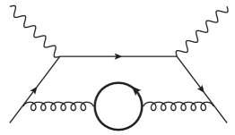
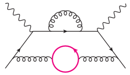
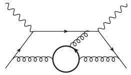
Figure 6: Sample Feynman diagrams containing closed loops with charm quarks. The same notation as in Fig. 1 is used.

At three-loop order, also another kind of diagrams contributes, namely those where the charm loop is connected to the heavy quark by three gluons (see Fig. 6). In the threshold limit, these diagrams factorize into on-shell or tadpole integrals, where the mass scales are given by the charm and bottom quarks, and integrals with ultra-soft loop momenta. For the bare three-loop diagrams, we obtain a non-trivial dependence on $m_{c}/m_{b}$. However, incorporating the proper on-shell counterterms for the wave function and heavy quark masses, only logarithmic contributions remain. These logarithmic contributions disappear if $\alpha_{s}^{(3)}$ is chosen as expansion parameter. Moreover, the non-logarithmic part of the resulting $n_{l}=3$ expression is identical to the one obtained for massless charm quarks.

To summarize, all charm quark mass effects in the $n_{l}=4$ flavour theory are decoupling effects. Thus, one can start the calculation in a theory where both charm and bottom quarks are integrated out. The transition from $\alpha_{s}^{(3)}$ to $\alpha_{s}^{(4)}$ generates $\ln(\mu_{\rm dec}^{2}/m_{c}^{2})$ terms, where $\mu_{\rm dec}$ is the scale where the charm quark is decoupled, and, at three-loop order, also constant contributions. The $m^{\rm kin}$–$m^{\rm OS}$ relation one obtains this way agrees with our explicit calculation in the four flavour theory, assuming the scaling $|y|\ll m_{c}^{2},m_{b}^{2}$.

Note that due to the definition of the kinetic mass in the heavy quark limit we are forced to choose $m_{c}=0$ in case we assume the scaling $m_{c}^{2}\sim|y|$, see also Ref. [15] for explicit results at order $\alpha_{s}^{2}$.

5 Analytic results

5.1 Renormalization

Before presenting analytic results for the quark mass relations, we want to discuss the renormalization of the parameters and the wave function of the external quarks. Note that the quantity we compute is infra-red finite.

At one-loop order there is no counterterm contribution to the imaginary part of the forward-scattering amplitude. In order to treat the ultra-violet divergences at two and three loops, we have to renormalize the strong coupling constant, the heavy quark wave function, the heavy quark mass and the mass parameter $m$ in the definition of the scalar current, see Eq. (34). We renormalize $\alpha_{s}$ in the $\overline{\rm MS}$-scheme. The on-shell wave function renormalization constant $Z_{2}^{\rm OS}$ is needed up to two-loop order [59, 62, 33] where also finite charm quark mass effects are needed [59, 60]. We choose to renormalize the scalar current in the $\overline{\rm MS}$-scheme to match the renormalization scheme used for the virtual corrections, cf. Eq. (46). The respective renormalization constant $Z_{m}^{\overline{\rm MS}}$ is needed up to two-loops. For the renormalization of the heavy quark mass, which is present in the virtual propagators, we introduce the corresponding counterterm in each one- and two-loop diagram and compute the corresponding higher order contributions together with bare contributions at the respective loop order. The renormalization constant $Z_{m}^{\rm OS}$ is again needed up to two loops [63], including finite charm quark mass contributions [64, 60]. Note that the heavy quark mass counterterms generate gauge depend terms which are needed in order to cancel the gauge dependence of the bare diagrams.

In our approach, we also generate diagrams which contain closed massive quark loops (bottom or charm), which means that all quarks contribute to the running of $\alpha_{s}$. To arrive at the theory with only $n_{f}-1$ light flavors, we apply the decoupling relation (see, e.g., Ref. [65])

$$\alpha_{s}^{(n_{f})}(\mu_{th}) = \alpha_{s}^{(n_{f}-1)}(\mu_{th})\Biggl{[}1+\frac{\alpha_{s}^{(n_{f}-1)}(\mu_{th})}{\pi}c_{1}\left(\frac{m}{\mu_{th}}\right)+\left(\frac{\alpha_{s}^{(n_{f}-1)}(\mu_{th})}{\pi}\right)^{2}c_{2}\left(\frac{m}{\mu_{th}}\right)\Biggr{]}\,,$$

where for later convenience we provide explicit results for the one- and two-loop coefficients

$$c_{1}\left(\frac{m}{\mu_{th}}\right) = \frac{1}{3}n_{h}T_{F}\ln\left(\frac{\mu_{th}^{2}}{m^{2}}\right)\,,$$ (60)

$$c_{2}\left(\frac{m}{\mu_{th}}\right) = n_{h}T_{F}\biggl{[}\frac{1}{9}n_{h}T_{F}\ln^{2}\left(\frac{\mu_{th}^{2}}{m^{2}}\right)+\left(\frac{5}{12}C_{A}-\frac{1}{4}C_{F}\right)\ln\left(\frac{\mu_{th}^{2}}{m^{2}}\right)-\frac{2}{9}C_{A}+\frac{15}{16}C_{F}\biggr{]}\,.$$

In the above formulae, $m$ denotes the on-shell mass. In case massive charm effects are considered, one first has to use Eq. (LABEL:eq::asdec) for the bottom and subsequently for the charm quark. Note that this is possible since up to two-loop order there are no genuine $m_{c}/m_{b}$ effects (see also Ref. [66]). Note that $c_{1}\sim\ln(m^{2}/\mu_{th}^{2})$ and thus $c_{1}(1)=0$. However, the two-loop term has a finite remainder, i.e. $c_{2}(1)\not=0$.

The renormalization of the structure functions shows some interesting features. At two loops the (uu) region is already finite after renormalization of the strong coupling constant. The (uh) region does only contribute to the $C_{F}^{2}$ and $C_{F}T_{F}n_{h}$ color factors but not to $C_{F}C_{A}$ and $C_{F}T_{F}n_{l}$. Furthermore, it has terms that scale as $\sim y^{-2}$. These terms are cancelled by the (on-shell) quark mass counterterms. After applying the wave function counterterm, the $C_{F}^{2}$ term is exactly cancelled for the vector current. In the scalar case, there is a residual $C_{F}^{2}$ term which cancels against the non-vanishing virtual corrections when calculating the kinetic mass relation. The remaining terms proportional to $n_{h}$ are eliminated by decoupling the heavy quarks from the running of $\alpha_{s}$.

Very similar observations can be made at three loops. The all-ultra-soft region (uuu) is finite after coupling constant renormalization. Here, the (uuh) and (uhh) regions scale up to $\sim y^{-3}$. Again these terms are cancelled by the heavy quark mass counterterms. In case finite charm quark mass effects are considered, the (uhh) region has a non-trivial dependence on $m_{c}/m_{b}$. After wave function renormalization these contributions, as well as the whole contributions to the color factors $C_{F}^{3}$ and $C_{F}^{2}C_{A}$, vanish for an external vector current. For an external scalar current, also the virtual corrections are needed to establish the cancellation. Moreover, the remaining terms proportional to $n_{h}$ are again absorbed by decoupling.

The above observations can be summarized as follows: both at two- and three-loop order after including all relevant counterterm contributions and after expressing the final result in terms of $\alpha_{s}^{(n_{l})}$, only the pure-ultra-soft contributions survive and all contributions proportional to $n_{h}$ vanish. This means that one could have performed the calculation from the beginning in the effective $n_{l}$-flavour QCD. Furthermore, at the step where the asymptotic expansion is applied only ultra-soft regions have to be considered. From the physical point of view this behaviour is expected since the kinetic mass is defined via the radiation of soft gluons from the heavy quark. Since in our “full-theory” approach the cancellation of the $n_{h}$ contribution is non-trivial, we consider it as a welcome consistency check for the correctness of our calculation.

5.2 Quark mass relations

In this subsection we discuss various relations between the different definitions of the heavy quark masses. We consider QCD with $n_{f}$ active flavours, where $n_{f}=5$ for bottom and $n_{f}=4$ for charm. Furthermore, we denote by $n_{l}$ the number of massless quarks. It is interesting to consider charm mass effects to the bottom mass relations where we have $n_{f}=5$ and $n_{l}=3$. Since one can consider different numbers of active quarks for the running of $\alpha_{s}$, we introduce $n_{r}$, i.e. the number of active quark flavors in the running of $\alpha_{s}$. Charm effects in the $\overline{\rm MS}$-on-shell relation can be found in Refs. [63] and [60, 34] to two- and three-loop accuracy, respectively. The charm mass effects in the $m^{\rm kin}$–$m^{\rm OS}$ relation were discussed in Section 4.

Let us in a first step present results for the relation between the kinetic and the on-shell mass, see Eq. (21). Up to three-loop order our results reads

$$\frac{m^{\text{kin}}}{m^{\text{OS}}} = 1+\frac{\alpha_{s}^{(n_{r})}}{\pi}\left[\frac{\mu}{m^{\text{OS}}}t^{(1,1)}+\frac{\mu^{2}}{\left(m^{\text{OS}}\right)^{2}}t^{(1,2)}\right]$$ (62)

$$\mbox{}+\left(\frac{\alpha_{s}^{(n_{r})}}{\pi}\right)^{2}\left[\frac{\mu}{m^{\text{OS}}}t^{(2,1)}+\frac{\mu^{2}}{\left(m^{\text{OS}}\right)^{2}}t^{(2,2)}+\delta_{n_{r},4}\,\Delta_{m_{c}}^{\rm kin,(2)}(m_{c}^{\text{OS}},m^{\text{OS}})\right]$$

$$\mbox{}+\left(\frac{\alpha_{s}^{(n_{r})}}{\pi}\right)^{3}\left[\frac{\mu}{m^{\text{OS}}}t^{(3,1)}+\frac{\mu^{2}}{\left(m^{\text{OS}}\right)^{2}}t^{(3,2)}+\delta_{n_{r},4}\,\Delta_{m_{c}}^{\rm kin,(3)}(m_{c}^{\text{OS}},m^{\text{OS}})\right]\,,$$

with

$$t^{(1,1)} = -\frac{4}{3}C_{F}\,,$$

$$t^{(1,2)} = -\frac{1}{2}C_{F}\,,$$

$$t^{(2,1)} = C_{F}\Biggl{[}C_{A}\biggl{(}-\frac{215}{27}+\frac{2\pi^{2}}{9}+\frac{22}{9}l_{\mu}\biggr{)}+n_{l}T_{F}\biggl{(}\frac{64}{27}-\frac{8}{9}l_{\mu}\biggr{)}\Biggr{]}\,,$$

$$t^{(2,2)} = C_{F}\Biggl{[}C_{A}\biggl{(}-\frac{91}{36}+\frac{\pi^{2}}{12}+\frac{11}{12}l_{\mu}\biggr{)}+n_{l}T_{F}\biggl{(}\frac{13}{18}-\frac{1}{3}l_{\mu}\biggr{)}\Biggr{]}\,,$$

$$t^{(3,1)} = C_{F}\Biggl{[}C_{A}^{2}\biggl{(}-\frac{130867}{1944}+\frac{511\pi^{2}}{162}+\frac{19\zeta_{3}}{2}-\frac{\pi^{4}}{18}+\biggl{(}\frac{2518}{81}-\frac{22\pi^{2}}{27}\biggr{)}l_{\mu}-\frac{121}{27}l_{\mu}^{2}\biggr{)}$$

$$\mbox{}+C_{A}n_{l}T_{F}\biggl{(}\frac{19453}{486}-\frac{104\pi^{2}}{81}-2\zeta_{3}+\biggl{(}-\frac{1654}{81}+\frac{8\pi^{2}}{27}\biggr{)}l_{\mu}+\frac{88}{27}l_{\mu}^{2}\biggr{)}$$

$$\mbox{}+C_{F}n_{l}T_{F}\biggl{(}\frac{11}{4}-\frac{4\zeta_{3}}{3}-\frac{2}{3}l_{\mu}\biggr{)}+n_{l}^{2}T_{F}^{2}\biggl{(}-\frac{1292}{243}+\frac{8\pi^{2}}{81}+\frac{256}{81}l_{\mu}-\frac{16}{27}l_{\mu}^{2}\biggr{)}\Biggr{]}\,,$$

$$t^{(3,2)} = C_{F}\Biggl{[}C_{A}^{2}\biggl{(}-\frac{96295}{5184}+\frac{445\pi^{2}}{432}+\frac{57\zeta_{3}}{16}-\frac{\pi^{4}}{48}+\biggl{(}\frac{2155}{216}-\frac{11\pi^{2}}{36}\biggr{)}l_{\mu}-\frac{121}{72}l_{\mu}^{2}\biggr{)}$$ (63)

$$\mbox{}+C_{A}n_{l}T_{F}\biggl{(}\frac{13699}{1296}-\frac{23\pi^{2}}{54}-\frac{3\zeta_{3}}{4}+\biggl{(}-\frac{695}{108}+\frac{\pi^{2}}{9}\biggr{)}l_{\mu}+\frac{11}{9}l_{\mu}^{2}\biggr{)}$$

$$\mbox{}+C_{F}n_{l}T_{F}\biggl{(}\frac{29}{32}-\frac{\zeta_{3}}{2}-\frac{1}{4}l_{\mu}\biggr{)}+n_{l}^{2}T_{F}^{2}\biggl{(}-\frac{209}{162}+\frac{\pi^{2}}{27}+\frac{26}{27}l_{\mu}-\frac{2}{9}l_{\mu}^{2}\biggr{)}\Biggr{]}\,,$$

where $l_{\mu}=\ln(2\mu/\mu_{s})$ and $\mu_{s}$ is the renormalization scale of the strong coupling constant $\alpha_{s}^{(n_{r})}(\mu_{s})$; $\mu$ is the Wilsonian cutoff. Note that $m^{\rm kin}$ on the r.h.s. of Eq. (21) has been replaced by $m^{\rm OS}$ by applying the $m^{\rm kin}$–$m^{\rm OS}$ relation iteratively. In Eqs. (62) and (63) we have $n_{l}=n_{r}=3$ for $m=m_{c}$ while for $m=m_{b}$ we have $n_{l}=3$ and $n_{r}=3$ or $4$.

$\Delta^{\rm kin,(2)}$ and $\Delta^{\rm kin,(3)}$ denote the two- and three-loop finite-$m_{c}$ corrections, respectively, which have to be taken into account if the bottom quark relation is considered for $n_{r}=4$. The analytic expressions are given by

$$\Delta_{m_{c}}^{\rm kin,(2)}(m_{c},m) = -c_{1}\left(\frac{m_{c}}{\mu_{s}}\right)\left[\frac{\mu}{m}t^{(1,1)}+\frac{\mu^{2}}{\left(m\right)^{2}}t^{(1,2)}\right]\,,$$

$$\Delta_{m_{c}}^{\rm kin,(3)}(m_{c},m) = \left[2\,c_{1}^{2}\left(\frac{m_{c}}{\mu_{s}}\right)-c_{2}\left(\frac{m_{c}}{\mu_{s}}\right)\right]\left[\frac{\mu}{m}t^{(1,1)}+\frac{\mu^{2}}{\left(m\right)^{2}}t^{(1,2)}\right]$$ (64)

$$\mbox{}-2\,c_{1}\left(\frac{m_{c}}{\mu_{s}}\right)\left[\frac{\mu}{m}t^{(2,1)}+\frac{\mu^{2}}{\left(m\right)^{2}}t^{(2,2)}\right]\,,$$

where we have identified the decoupling scale $\mu_{th}$ with $\mu_{s}$. Note that these corrections are pure decoupling effects and are absent for $n_{r}=3$. The functions $c_{1}\left(m/\mu_{th}\right)$ and $c_{2}\left(m/\mu_{th}\right)$ are given in Eqs. (60) and (LABEL:eq:decoupling2), respectively.

For convenience of the reader, we also present the inverted relation which allows for the computation of the on-shell mass from the kinetic mass:

$$\frac{m^{\text{OS}}}{m^{\text{kin}}} = 1-\frac{\alpha_{s}^{(n_{r})}}{\pi}\left[\frac{\mu}{m^{\text{kin}}}t^{(1,1)}+\frac{\mu^{2}}{\left(m^{\text{kin}}\right)^{2}}t^{(1,2)}\right]$$ (65)

$$\mbox{}-\left(\frac{\alpha_{s}^{(n_{r})}}{\pi}\right)^{2}\left[\frac{\mu}{m^{\text{kin}}}t^{(2,1)}+\frac{\mu^{2}}{\left(m^{\text{kin}}\right)^{2}}t^{(2,2)}+\delta_{n_{r},4}\,\Delta_{m_{c}}^{\rm kin,(2)}(m_{c}^{\text{OS}},m^{\text{kin}})\right]$$

$$\mbox{}-\left(\frac{\alpha_{s}^{(n_{r})}}{\pi}\right)^{3}\Biggl{\{}\frac{\mu}{m^{\text{kin}}}t^{(3,1)}+\frac{\mu^{2}}{\left(m^{\text{kin}}\right)^{2}}t^{(3,2)}+\delta_{n_{r},4}\Delta_{m_{c}}^{\rm kin,(3)}(m_{c}^{\text{OS}},m^{\text{kin}})\Biggr{\}}\,.$$

Note that in the case of the charm quark we always have $n_{l}=n_{r}=3$.

Next we want to consider the relation between the kinetic and the $\overline{\rm MS}$ mass of the bottom quark. In order to keep the formula compact, we choose to work with $n_{r}=4$ active flavors for the running of $\alpha_{s}$. In section 7 we will refer to this choice as scheme (B). To obtain this relation, we replace the pole mass on the r.h.s. of (64) by the $\overline{\rm MS}$ mass using the corresponding three-loop relation [67, 30, 32]. We choose a common renormalization scale $\mu_{s}$ for $\alpha_{s}$, $\overline{m}_{b}$ and $\overline{m}_{c}$. In the $m^{\rm OS}_{b}$–$\overline{m}_{b}$ relation, we replace $\alpha_{s}^{(n_{f}=5)}$ in favour of $\alpha_{s}^{(4)}$ to have the same expansion parameter as in Eqs. (64) and (65). The corresponding formula reads

$$m_{b}^{\text{OS}} = \overline{m}_{b}(\mu_{s})\Biggl{[}1+\frac{\alpha_{s}^{(4)}}{\pi}y_{m}^{(1)}+\left(\frac{\alpha_{s}^{(4)}}{\pi}\right)^{2}\left(y_{m}^{(2)}+\Delta_{m_{c}}^{(2)}\right)+\left(\frac{\alpha_{s}^{(4)}}{\pi}\right)^{3}\left(y_{m}^{(3)}+\Delta_{m_{c}}^{(3)}\right)\Biggr{]}\,,$$

with

$$y_{m}^{(1)} = C_{F}\left(1+\frac{3}{4}l_{m}\right)\,,$$

$$y_{m}^{(2)} = C_{A}C_{F}\biggl{[}\frac{1111}{384}-\frac{3}{8}\zeta_{3}+\frac{\pi^{2}}{12}\big{(}3l_{2}-1\big{)}+\frac{185l_{m}}{96}+\frac{11l_{m}^{2}}{32}\biggr{]}$$

$$\mbox{}+C_{F}T_{F}\biggl{[}-\frac{107}{48}+\frac{\pi^{2}}{12}-\frac{3l_{m}}{4}-n_{l}\biggl{(}\frac{71}{96}+\frac{\pi^{2}}{12}+\frac{13l_{m}}{24}+\frac{l_{m}^{2}}{8}\biggr{)}\biggr{]}$$

$$\mbox{}+C_{F}^{2}\biggl{[}-\frac{71}{128}+\frac{3}{4}\zeta_{3}+\frac{\pi^{2}}{16}\big{(}5-8l_{2}\big{)}-\frac{9l_{m}}{32}+\frac{9l_{m}^{2}}{32}\biggr{]}\,,$$

$$y_{m}^{(3)} = C_{F}^{2}T_{F}\Biggl{\{}-\frac{397}{144}-\frac{16a_{4}}{3}+\frac{7\pi^{4}}{540}+n_{l}\biggl{[}-\frac{109}{72}-\frac{8a_{4}}{3}+\frac{119\pi^{4}}{2160}-\pi^{2}\biggl{(}\frac{55}{72}+\frac{2l_{2}^{2}}{9}$$

$$\mbox{}+\frac{13l_{m}}{48}-\frac{1}{9}l_{2}\bigl{(}11+3l_{m}\bigr{)}\biggr{)}-\frac{55}{24}\zeta_{3}-\frac{l_{2}^{4}}{9}+\biggl{(}-\frac{91}{384}+\frac{\zeta_{3}}{4}\biggr{)}l_{m}-\frac{3l_{m}^{2}}{32}-\frac{3l_{m}^{3}}{32}\biggr{]}$$

$$\mbox{}+\pi^{2}\biggl{[}\frac{23}{216}-\frac{l_{2}^{2}}{9}-\frac{7l_{m}}{48}+\frac{1}{3}l_{2}\bigl{(}1+l_{m}\bigr{)}\biggr{]}-\frac{1}{12}\zeta_{3}-\frac{2l_{2}^{4}}{9}+\biggl{(}-\frac{93}{64}+\zeta_{3}\biggr{)}l_{m}-\frac{9l_{m}^{2}}{16}\Biggr{\}}$$

$$\mbox{}+C_{A}C_{F}T_{F}\Biggl{\{}-\frac{109589}{7776}+\frac{8a_{4}}{3}+\frac{67\pi^{4}}{2160}+\pi^{2}\biggl{[}\frac{293}{108}-\frac{1}{8}\zeta_{3}+\frac{l_{2}^{2}}{18}-\frac{l_{2}}{6}\bigl{(}25+l_{m}\bigr{)}$$

$$\mbox{}+\frac{5l_{m}}{24}\biggr{]}+n_{l}\biggl{[}-\frac{70763}{15552}+\frac{4a_{4}}{3}-\frac{19\pi^{4}}{2160}+\pi^{2}\biggl{(}-\frac{175}{432}+\frac{l_{2}^{2}}{9}-\frac{l_{2}}{18}\bigl{(}11+3l_{m}\bigr{)}-\frac{7l_{m}}{72}\biggr{)}$$

$$\mbox{}-\frac{89}{144}\zeta_{3}+\frac{l_{2}^{4}}{18}-\biggl{(}\frac{869}{216}+\frac{\zeta_{3}}{2}\biggr{)}l_{m}-\frac{373l_{m}^{2}}{288}-\frac{11l_{m}^{3}}{72}\biggr{]}+\frac{5}{36}\zeta_{3}+\frac{5}{8}\zeta_{5}+\frac{l_{2}^{4}}{9}$$

$$\mbox{}-\biggl{(}\frac{12515}{1728}+\frac{5\zeta_{3}}{4}\biggr{)}l_{m}-\frac{143l_{m}^{2}}{144}-\frac{11l_{m}^{3}}{144}\Biggr{\}}+C_{F}T_{F}^{2}\Biggl{\{}\frac{5917}{1944}+n_{l}\biggl{(}\frac{4135}{1944}+\frac{13\pi^{2}}{108}$$

$$\mbox{}+\frac{5}{9}\zeta_{3}+\frac{715l_{m}}{432}+\frac{13l_{m}^{2}}{36}+\frac{l_{m}^{3}}{36}\biggr{)}+n_{l}^{2}\biggl{(}\frac{2353}{7776}+\frac{7}{18}\zeta_{3}+\frac{89l_{m}}{216}+\frac{13l_{m}^{2}}{72}+\frac{l_{m}^{3}}{36}$$

$$\mbox{}+\frac{\pi^{2}}{108}\bigl{(}13+6l_{m}\bigr{)}\biggr{)}-\frac{4}{9}\zeta_{3}-\frac{\pi^{2}}{270}\bigl{(}8+15l_{m}\bigr{)}+\frac{251l_{m}}{216}+\frac{l_{m}^{2}}{9}+\frac{l_{m}^{3}}{36}\Biggr{\}}$$

$$\mbox{}+C_{F}^{3}\Biggl{\{}\frac{893}{192}+12a_{4}+\frac{\pi^{4}}{48}+\pi^{2}\biggl{(}\frac{643}{192}+\frac{1}{16}\zeta_{3}-\frac{l_{2}^{2}}{2}+\frac{15l_{m}}{64}-\frac{3}{8}l_{2}\bigl{(}20+l_{m}\bigr{)}\biggr{)}$$

$$\mbox{}+\frac{87}{16}\zeta_{3}-\frac{5}{8}\zeta_{5}+\frac{l_{2}^{4}}{2}+\biggl{(}\frac{495}{512}+\frac{9\zeta_{3}}{16}\biggr{)}l_{m}-\frac{63l_{m}^{2}}{128}+\frac{9l_{m}^{3}}{128}\Biggr{\}}+C_{A}^{2}C_{F}\Biggl{\{}\frac{1322545}{124416}$$

$$\mbox{}-\frac{11a_{4}}{3}+\frac{179\pi^{4}}{3456}+\pi^{2}\biggl{(}\frac{1955}{3456}-\frac{51}{64}\zeta_{3}-\frac{11l_{2}^{2}}{36}-\frac{11l_{m}}{72}+\frac{1}{72}l_{2}\bigl{(}115+33l_{m}\bigr{)}\biggr{)}$$

$$\mbox{}-\frac{1343}{288}\zeta_{3}+\frac{65}{32}\zeta_{5}-\frac{11l_{2}^{4}}{72}+\biggl{(}\frac{13243}{1728}-\frac{11\zeta_{3}}{16}\biggr{)}l_{m}+\frac{2341l_{m}^{2}}{1152}+\frac{121l_{m}^{3}}{576}\Biggr{\}}$$

$$\mbox{}+C_{A}C_{F}^{2}\Biggl{\{}-\frac{24283}{4608}+\frac{4a_{4}}{3}-\frac{65\pi^{4}}{432}+\pi^{2}\biggl{(}-\frac{533}{576}+\frac{19}{16}\zeta_{3}+\frac{31l_{2}^{2}}{36}+\frac{49l_{m}}{96}$$

$$\mbox{}+\frac{5}{144}l_{2}\bigl{(}16-21l_{m}\bigr{)}\biggr{)}+\frac{755}{96}\zeta_{3}-\frac{45}{16}\zeta_{5}+\frac{l_{2}^{4}}{18}-\biggl{(}\frac{4219}{1536}-\frac{35\zeta_{3}}{32}\biggr{)}l_{m}$$

$$\mbox{}+\frac{21l_{m}^{2}}{64}+\frac{33l_{m}^{3}}{128}\Biggr{\}}\,,$$

$$\Delta_{m_{c}}^{(2)} = C_{F}T_{F}\biggl{[}-\frac{3z^{2}}{4}+\frac{\pi^{2}}{12}z\bigl{(}3+3z^{2}-z^{3}\bigr{)}+\frac{1}{2}\biggl{(}(1-z)^{2}\big{(}1+z+z^{2}\big{)}\ln(1-z)$$

$$\mbox{}+(1+z)^{2}\big{(}1-z+z^{2}\big{)}\ln(1+z)-z^{2}\biggr{)}\ln(z)-\frac{1}{2}z^{4}\ln^{2}(z)$$

$$\mbox{}+\frac{1}{2}(1+z)^{2}\big{(}1-z+z^{2}\big{)}\text{Li}_{2}(-z)+\frac{1}{2}(1-z)^{2}\big{(}1+z+z^{2}\big{)}\text{Li}_{2}(z)\biggr{]}\,,$$

$$\Delta_{m_{c}}^{(3)} = \biggl{[}\frac{1}{2}C_{F}+\frac{2}{3}T_{F}l_{m}\biggr{]}\Delta_{m_{c}}^{(2)}+C_{F}^{2}T_{F}l_{c}\biggl{[}-\frac{3z^{2}}{2}+\frac{1}{16}\pi^{2}z\big{(}3+9z^{2}-4z^{3}\big{)}$$ (67)

$$\mbox{}+\frac{3}{8}z(1+z)\big{(}1-z+4z^{2}\big{)}\text{Li}_{2}(-z)-\frac{3}{8}z(1-z)\big{(}1+z+4z^{2}\big{)}\text{Li}_{2}(z)$$

$$\mbox{}+\biggl{(}-\frac{3z^{2}}{4}-\frac{3}{8}z(1-z)\big{(}1+z+4z^{2}\big{)}\ln(1-z)$$

$$\mbox{}+\frac{3}{8}z(1+z)\big{(}1-z+4z^{2}\big{)}\ln(1+z)\biggr{)}\ln(z)-\frac{3}{2}z^{4}\ln^{2}(z)\biggr{]}$$

$$\mbox{}+C_{F}^{2}T_{F}l_{m}\biggl{[}\frac{3z^{2}}{8}+\frac{1}{16}\pi^{2}z\big{(}3-3z^{2}+2z^{3}\big{)}+\frac{3}{4}z^{4}\ln^{2}(z)$$

$$\mbox{}+\frac{3}{8}(1-z^{2})\big{(}2-z+2z^{2}\big{)}\biggl{(}\ln(1-z)\ln(z)+\text{Li}_{2}(z)\biggr{)}$$

$$\mbox{}+\frac{3}{8}(1-z^{2})\big{(}2+z+2z^{2}\big{)}\biggl{(}\ln(1+z)\ln(z)+\text{Li}_{2}(-z)\biggr{)}\biggr{]}-\tilde{\Delta}_{m_{c}}^{(3)}\,,$$

where

$$z =\frac{\overline{m}_{c}}{\overline{m}_{b}}\,, l_{m} =\ln\left(\frac{\mu_{s}^{2}}{\overline{m}_{b}^{2}}\right)\,, l_{c} =\ln\left(\frac{\mu_{s}^{2}}{\overline{m}_{c}^{2}}\right)\,,$$

$$l_{2} =\ln\left(2\right)\,, a_{4} =\text{Li}_{4}\left(\frac{1}{2}\right)\,.$$ (68)

The contributions due to charm quark mass are taken from Ref. [34]. The term $\tilde{\Delta}_{m_{c}}^{(3)}$ denotes the genuine three loop contribution, which vanishes for $m_{c}\to 0$. It can be extracted from the ancillary file of Ref. [34]:

$$\tilde{\Delta}_{m_{c}}^{(3)} = \left.\texttt{zmnum}[x,\overline{m}_{b},\mu_{s},\mu_{s}]-\lim_{x\to 0}\texttt{zmnum}[x,\overline{m}_{b},\mu_{s},\mu_{s}]\right|_{\alpha_{s}^{3}}\,.$$ (69)

Alternatively, also the corresponding analytic expressions provided in [34] can be used.

After expanding in $\alpha_{s}^{(4)}(\mu_{s})$ up to third order and $\mu/\overline{m}$ up to second order, we obtain the relation between the kinetic and the $\overline{\text{MS}}$ mass of the bottom quark:

$$\frac{m^{\rm kin}_{b}(\mu)}{\overline{m}_{b}} = 1+\frac{\alpha_{s}^{(4)}}{\pi}\biggl{[}y_{m}^{(1)}+\frac{\mu}{\overline{m}_{b}}t^{(1,1)}+\frac{\mu^{2}}{\overline{m}_{b}^{2}}t^{(1,2)}\biggr{]}$$ (70)

$$\mbox{}+\left(\frac{\alpha_{s}^{(4)}}{\pi}\right)^{2}\Biggl{[}y_{m}^{(2)}+\Delta_{m_{c}}^{(2)}+\frac{\mu}{\overline{m}_{b}}t^{(2,1)}+\frac{\mu^{2}}{\overline{m}_{b}^{2}}\biggl{(}t^{(2,2)}-y_{m}^{(1)}t^{(1,2)}\biggr{)}$$

$$\mbox{}+\Delta_{m_{c}}^{\rm kin,(2)}(\overline{m}_{c},\overline{m}_{b})\Biggr{]}+\left(\frac{\alpha_{s}^{(4)}}{\pi}\right)^{3}\Biggl{[}y_{m}^{(3)}+\Delta_{m_{c}}^{(3)}+\frac{\mu}{\overline{m}_{b}}t^{(3,1)}$$

$$\mbox{}+\frac{\mu^{2}}{\overline{m}_{b}^{2}}\Biggl{(}t^{(3,2)}-y_{m}^{(1)}t^{(2,2)}-t^{(1,2)}\biggl{(}y_{m}^{(2)}+\Delta_{m_{c}}^{(2)}-\left(y_{m}^{(1)}\right)^{2}\biggr{)}\Biggr{)}$$

$$\mbox{}+\Delta_{m_{c}}^{\rm kin,(3)}(\overline{m}_{c},\overline{m}_{b})+y_{m}^{(1)}\Delta_{m_{c}}^{\rm kin,(2)}(\overline{m}_{c},\overline{m}_{b})+\frac{\mu}{\overline{m}_{b}}t^{(1,1)}\biggl{(}c_{1}\left(\frac{\overline{m}_{c}}{\mu_{s}}\right)y_{m}^{(1)}$$

$$\mbox{}+\frac{2}{3}T_{F}y_{m_{c}}^{(1)}\biggr{)}+\frac{\mu^{2}}{\overline{m}_{b}^{2}}t^{(1,2)}\biggl{(}2c_{1}\left(\frac{\overline{m}_{c}}{\mu_{s}}\right)y_{m}^{(1)}+\frac{2}{3}T_{F}y_{m_{c}}^{(1)}\biggr{)}\Biggr{]}\,,$$

with

$$y_{m_{c}}^{(1)} = C_{F}\left(1+\frac{3}{4}l_{c}\right)\,,$$ (71)

$\overline{m}_{b}=\overline{m}_{b}(\mu_{s})$, $\overline{m}_{c}=\overline{m}_{c}(\mu_{s})$ as well as $\alpha_{s}^{(4)}=\alpha_{s}^{(4)}(\mu_{s})$. The inverted relation $\overline{m}_{b}/m^{\rm kin}_{b}(\mu)$ is obtained from Eq. (70) in a straightforward way. We refrain from printing it in the paper but refer to the ancillary files [57] where also the relations between the kinetic and on-shell mass can be found.

6 BLM corrections to four loops

In this section we present the four-loop contribution to the $m^{\rm OS}$–$m^{\rm kin}$ relation for the class of diagrams that contain three insertions of massless fermion bubbles in a gluon propagator. Such corrections are usually referred to as “large-$\beta_{0}$” (or “BLM” [68]) corrections, see also [69]. Often one performs the replacement

$$n_{l} \to -\frac{3}{2}\beta_{0}\,,$$ (72)

with $\beta_{0}=11C_{A}/3-4T_{F}n_{l}/3$ and uses these corrections to estimate unknown higher order contributions. We adopt this approach in order to get a hint about the size of the ${O}(\alpha_{s}^{4})$ corrections.

Let us have a brief look to the large-$\beta_{0}$ corrections at two- and three-loop order. We consider the $m_{b}^{\rm kin}$-$\overline{m}_{b}$ relation and obtain at two and three loops the following large-$\beta_{0}$ terms:

$$m_{b}^{\rm kin}(1~{}\mbox{GeV}) = 4163+248+(-57+137|_{{\rm large}-\beta_{0}})+(15+15|_{{\rm large}-\beta_{0}})\,.$$ (73)

One observes that at ${O}(\alpha_{s}^{2})$ the large-$\beta_{0}$ term is about twice as big as the remaining contribution, however, it has a different sign. Thus, it overshoots the full result by a factor of two. At three-loop order, the large-$\beta_{0}$ term amounts to half of the complete result.

The leading $n_{l}^{n}$ term at order $(n+1)$ can be obtained by dressing the gluon propagator in each of the four one-loop diagrams with $n$ closed (massless) fermion loops. The bubbles can be integrated out which leads to an effective gluon propagator raised to a symbolic power. In fact, if we denote the momentum through the gluon line by $k_{1}$ it is sufficient to perform the simple replacement

$$\frac{-g^{\rho\sigma}}{[-k_{1}^{2}]} \to \frac{-g^{\rho\sigma}}{[-k_{1}^{2}]}\left(8\Gamma(2-d/2)\frac{\Gamma^{2}(d/2)}{\Gamma(d)}\frac{1}{[k_{1}^{2}]^{2-d/2}}\right)^{n}\,,$$ (74)

in order to obtain the $n_{l}^{n}$ contribution at order $\alpha_{s}^{n+1}$. It is straightforward to obtain analytic results for any given value of $n$. Our interest is for $n=3$ which gives

$$\left.\frac{m^{\rm kin}}{m^{\text{OS}}}\right|_{\alpha_{s}^{4},BLM} = C_{F}\beta_{0}^{3}\Biggl{[}\frac{\mu}{m^{\text{OS}}}\biggl{(}-\frac{4069}{648}+\frac{2\pi^{2}}{9}+\frac{\zeta_{3}}{4}+\left(\frac{323}{72}-\frac{\pi^{2}}{12}\right)l_{\mu}-\frac{4}{3}l_{\mu}^{2}+\frac{1}{6}l_{\mu}^{3}\biggr{)}$$ (75)

$$+\frac{\mu^{2}}{\left(m^{\text{OS}}\right)^{2}}\biggl{(}-\frac{4205}{3456}+\frac{13\pi^{2}}{192}+\frac{3\zeta_{3}}{32}+\left(\frac{209}{192}-\frac{\pi^{2}}{32}\right)l_{\mu}$$

$$-\frac{13}{32}l_{\mu}^{2}+\frac{1}{16}l_{\mu}^{3}\biggr{)}\Biggr{]}\left(\frac{\alpha_{s}}{\pi}\right)^{4}\,,$$

with $l_{\mu}=\ln(2\mu/\mu_{s})$, where the counterterms for the strong coupling constant have been obtained from the known lower-order results.

Next we combine Eq. (75) with the corresponding terms from the $\overline{\text{MS}}$-on-shell relation [70, 71] and obtain

$$\left.\frac{m^{\rm kin}}{\overline{m}}\right|_{\alpha_{s}^{4},BLM} = C_{F}\beta_{0}^{3}\Biggl{[}\frac{42979}{442368}+\frac{89\pi^{2}}{1536}+\frac{317\zeta_{3}}{1024}+\frac{71\pi^{4}}{10240}+\left(\frac{1301}{9216}+\frac{13\pi^{2}}{256}+\frac{9\zeta_{3}}{64}\right)l_{m}$$ (76)

$$+\left(\frac{89}{1024}+\frac{3\pi^{2}}{256}\right)l_{m}^{2}+\frac{13}{512}l_{m}^{3}+\frac{3}{1024}l_{m}^{4}+\frac{\mu}{\overline{m}}\biggl{(}-\frac{4069}{648}+\frac{2\pi^{2}}{9}+\frac{\zeta_{3}}{4}$$

$$+\left(\frac{323}{72}-\frac{\pi^{2}}{12}\right)l_{\mu}-\frac{4}{3}l_{\mu}^{2}+\frac{1}{6}l_{\mu}^{3}\biggr{)}+\frac{\mu^{2}}{\overline{m}^{2}}\biggl{(}-\frac{4205}{3456}+\frac{13\pi^{2}}{192}+\frac{3\zeta_{3}}{32}$$

$$+\left(\frac{209}{192}-\frac{\pi^{2}}{32}\right)l_{\mu}-\frac{13}{32}l_{\mu}^{2}+\frac{1}{16}l_{\mu}^{3}\biggr{)}\Biggr{]}\left(\frac{\alpha_{s}}{\pi}\right)^{4}\,,$$

with $l_{m}=\ln(\mu_{s}^{2}/\overline{m}^{2})$.

We anticipate that the numerical effect is small for the bottom quark: for $\mu=1$ GeV, $\mu_{s}=\overline{m}$, $\overline{m}=4.163$ GeV and $n_{l}=3$ we obtain a contribution of about $-9$ MeV to $m^{\rm kin}$ in Eq. (76).

7 Numerical results

The input values for our numerical analysis are $\alpha_{s}^{(5)}(M_{Z})=0.1179$ [72], $\overline{m}_{c}(3~{}\mbox{GeV})=0.993$ GeV [6] and $\overline{m}_{b}(\overline{m}_{b})=4.163$ GeV [73]. We use RunDec [20] for the running of the $\overline{\rm MS}$ parameters and the decoupling of heavy particles. For the Wilsonian cutoff we choose $\mu=1$ GeV for bottom [74] and $\mu=0.5$ GeV or $\mu=1$ GeV for charm [75].

7.1 Charm mass

Let us start with the charm quark where we have $n_{l}=3$. Often numerical values for $\overline{m}_{c}(\overline{m}_{c})$ are provided. However, this choice suffers from small renormalization scales of the order 1 GeV. A more appropriate choice is thus $\overline{m}_{c}(2~{}\mbox{GeV})$ or $\overline{m}_{c}(3~{}\mbox{GeV})$. For the three choices we obtain the following perturbative expansions for $m_{c}^{\rm kin}(0.5~{}\mbox{GeV})$:

$$m_{c}^{\rm kin}(0.5~{}\mbox{GeV}) = \hphantom{0}993+191+100+52~{}\mbox{MeV}=1336~{}\mbox{MeV}\,,$$

$$m_{c}^{\rm kin}(0.5~{}\mbox{GeV}) = 1099+163+\hphantom{0}76+34~{}\mbox{MeV}=1372~{}\mbox{MeV}\,,$$

$$m_{c}^{\rm kin}(0.5~{}\mbox{GeV}) = 1279+\hphantom{0}84+\hphantom{0}30+11~{}\mbox{MeV}=1404~{}\mbox{MeV}\,.$$ (77)

For $m_{c}^{\rm kin}(1~{}\mbox{GeV})$ we obtain:

$$m_{c}^{\rm kin}(1~{}\mbox{GeV}) = \hphantom{0}993+83+35+14~{}\mbox{MeV}=1125~{}\mbox{MeV}\,,$$

$$m_{c}^{\rm kin}(1~{}\mbox{GeV}) = 1099+37+\hphantom{0}2-\hphantom{0}3~{}\mbox{MeV}=1135~{}\mbox{MeV}\,,$$

$$m_{c}^{\rm kin}(1~{}\mbox{GeV}) = 1279-73-61-17~{}\mbox{MeV}=1128~{}\mbox{MeV}\,,$$ (78)

where, from top to bottom, $\mu_{s}=3~{}\mbox{GeV},2~{}\mbox{GeV}$ and $\overline{m}_{c}$ was chosen for $\overline{m}_{c}(\mu_{s})$ and $\alpha_{s}(\mu_{s})$. Within each equation, the four numbers after the first equality sign refer to the tree-level results and the one-, two- and three-loop corrections. One observes that for each choice of $\mu_{s}$ the perturbative expansion behaves reasonably. It is interesting to mention that for $\mu_{s}=2~{}\mbox{GeV}$ and $\mu=1~{}\mbox{GeV}$ both the two- and three-loop corrections are particularly small and have different signs. For this choice of $\mu$, we also observe that with $\mu_{s}=3~{}\mbox{GeV}$ the loop corrections are positive, whereas for $\mu_{s}=\overline{m}_{c}$ they are negative. The three-loop terms range from $+14$ MeV to $-17$ MeV and roughly cover the splitting of the final numbers for $m_{c}^{\rm kin}(1~{}\mbox{GeV})$. For $\mu=0.5~{}\mbox{GeV}$ the three-loop terms range from $10$ MeV to $52$ MeV which again covers the splitting of the final numbers for $m_{c}^{\rm kin}(0.5~{}\mbox{GeV})$.

7.2 Bottom mass

Let us in the following investigate the numerical effects for the bottom quark including finite charm mass effects. In principle one has two choices for the treatment of $m_{c}$: one can either assume that $m_{c}\sim m_{b}$ and thus we have $m_{c}^{2}\gg|y|$. This leads to the results discussed in Section 4, i.e., the charm mass effects in the $m^{\rm kin}_{b}$–$m^{\rm OS}_{b}$ relation are given by the decoupling terms in $\alpha_{s}$. On the other hand, if the limit $m_{c}^{2}\ll m_{b}^{2}$ is considered in the $m^{\rm kin}_{b}$–$m^{\rm OS}_{b}$ relation, we are forced to set $m_{c}=0$. This is because due to the various limits involved in the definition of the kinetic mass there is no energy available to produce massive charm quarks. This means there is no expansion in $m_{c}/m_{b}$.

In the following we consider four schemes for the treatment of $m_{c}$ effects:

• We parametrize the $\overline{m}_{b}$–$m^{\rm kin}_{b}$ relation in terms of $\alpha_{s}^{(3)}$, i.e., we assume that the charm quark is decoupled and that there are no $m_{c}$ effects in the $m^{\rm kin}_{b}$–$m^{\rm OS}_{b}$ relation. Charm quark mass effects only come from the $\overline{m}_{b}$–$m^{\rm OS}_{b}$ relation. They are contained in the $\Delta_{m_{c}}^{(k)}$ ($k=2,3$) terms, which vanish in the limit $m_{c}\to 0$, and from decoupling effects in the transition from $\alpha_{s}^{(4)}$ to $\alpha_{s}^{(3)}$ in the $\overline{m}_{b}$–$m^{\rm OS}_{b}$ relation.

• We parametrize the $\overline{m}_{b}$–$m^{\rm kin}_{b}$ relation in terms of $\alpha_{s}^{(4)}$. The corresponding expression is obtained from scheme (A) by using the decoupling relations for $\alpha_{s}$. The charm quark mass effects are contained in the quantities $\Delta_{m_{c}}^{(k)}$ and $\Delta_{m_{c}}^{\rm kin,(k)}$ which originate from the $\overline{m}_{b}$–$m^{\rm OS}_{b}$ and $m^{\rm kin}_{b}$–$m^{\rm OS}_{b}$ relations, respectively.

• We parametrize the $\overline{m}_{b}$–$m^{\rm kin}_{b}$ relation in terms of $\alpha_{s}^{(4)}$ but assume that $m_{c}^{2}\ll|y|$. Note that this requires that $n_{l}=4$ has to be chosen in the $m^{\rm kin}_{b}$–$m^{\rm OS}_{b}$ relation (whereas in all other scheme we have $n_{l}=3$).

• We assume that the charm quark is formally infinitely heavy, in particular heavier than the bottom quark mass. In that case, we choose $n_{l}=3$ (similarly to scheme (A)) but we do not take into account any charm quark mass effect, neither from the decoupling in the $\alpha_{s}^{(4)}$ to $\alpha_{s}^{(3)}$ transition, nor from $\Delta_{m_{c}}^{(k)}$ in deriving the formulae for the mass relation.

As compared to the schemes used in Ref. [16], we include finite-$m_{c}$ effects. Note that in [16] the decoupling effects in the relation between $\alpha_{s}^{(4)}$ and $\alpha_{s}^{(3)}$ for the $\overline{m}_{b}$–$m^{\rm OS}_{b}$ have been neglected; they are relevant for scheme (A). The analytic result for scheme (B) can be found in Eq. (70). The formulae for the other schemes can be obtained from Eq. (70) in a straightforward way.

First, we use $\overline{m}_{b}(\overline{m}_{b})$ as input to compute the kinetic mass. We fix $\mu_{s}=\overline{m}_{b}$ but organize our formulae such that the scale of $\overline{m}_{c}$ is fixed to 3 GeV. For the four schemes we obtain

$$\mbox{(A)}\qquad m_{b}^{\rm kin}(1~{}\mbox{GeV}) = 4163+248+(81+7_{\Delta_{m_{c}}}+12_{dec}-20_{n_{c}})$$

$$\mbox{}+(30+14_{\Delta_{m_{c}}}+16_{dec}-30_{n_{c}}-1_{n_{c}\times dec}+0.4_{\Delta_{m_{c}}\times dec})~{}\mbox{MeV}$$

$$= 4163+248+80+30~{}\mbox{MeV}=4520~{}\mbox{MeV}\,,$$

$$\mbox{(B)}\qquad m_{b}^{\rm kin}(1~{}\mbox{GeV}) = 4163+259+(88+7_{\Delta_{m_{c}}}+5_{\Delta_{m_{c}}^{\rm kin}}-22_{n_{c}})$$

$$\mbox{}+(34+16_{\Delta_{m_{c}}}+10_{\Delta_{m_{c}}^{\rm kin}}-34_{n_{c}})~{}\mbox{MeV}$$

$$= 4163+259+78+26~{}\mbox{MeV}=4526~{}\mbox{MeV}\,,$$

$$\mbox{(C)}\qquad m_{b}^{\rm kin}(1~{}\mbox{GeV}) = 4163+259+(99+7_{\Delta_{m_{c}}}-22_{n_{c}})+(59+16_{\Delta_{m_{c}}}-34_{n_{c}})~{}\mbox{MeV}$$

$$= 4163+259+84+41~{}\mbox{MeV}=4547~{}\mbox{MeV}\,,$$

$$\mbox{(D)}\qquad m_{b}^{\rm kin}(1~{}\mbox{GeV}) = 4163+248+81+30~{}\mbox{MeV}=4521~{}\mbox{MeV}\,,$$ (79)

where the origins of the charm quark mass effects have been marked with the following labels.

• $dec$: it is present in scheme (A) and marks the terms in the $\overline{\rm MS}$-on-shell relation which originate from the decoupling of the charm quark in $\alpha_{s}$.

• $n_{c}$: the contribution from closed charm loops (which survive even for $m_{c}=0$).

• $\Delta_{m_{c}}$: finite $m_{c}$ terms from the $\overline{\rm MS}$-on-shell relation which vanish at $m_{c}=0$.

• $\Delta_{m_{c}}^{\rm kin}$: finite $m_{c}$ terms from the kinetic-on-shell relation

Overall, we observe that the charm mass effects from the $\overline{m}_{b}$–$m^{\rm OS}_{b}$ relation ($\Delta_{m_{c}}$) are sizeable and the three-loop term is about a factor of two bigger than the two-loop contribution. The same is true for the charm mass effects from the $m^{\rm kin}_{b}$–$m^{\rm OS}_{b}$ relation ($\Delta_{m_{c}}^{\rm kin}$ in scheme (B)). For scheme (A), the decoupling terms of $\alpha_{s}$ in the $\overline{m}_{b}$–$m^{\rm OS}_{b}$ relation also provide relatively large correction. However, for scheme (A) and (B), we see an important cancellation of these charm mass effects against the remaining $n_{c}$ terms that have the opposite sign as the previous three contributions. In scheme (C) the cancellation between $\Delta_{m_{s}}$ and $n_{c}$ is less efficient.

In the schemes (A), (B) and (D), one observes a good convergence of the perturbative series: the coefficients reduce by a factor two to three when going to higher orders. Scheme (C) behaves slightly worse. In our opinion, schemes (A) and (B) are the preferable choices for the phenomenological applications. The difference in the final results for the kinetic mass is only 6 MeV. The comparison between schemes (A), (B) and (D) demonstrates that the charm quark “wants” to be treated as a heavy particle. Note that the final result for scheme (D) differs from scheme (A) by only 1 MeV.

On the contrary, treating the charm as a light quark as in scheme (C) leads to a kinetic mass which is about 20 MeV larger than in the other schemes which is mainly due to the finite charm quark mass effects in the $\overline{\rm MS}$-on-shell relation. In this case, there is no room for a finite charm quark mass in the kinetic-on-shell relation. Note, however, that $m_{c}^{2}\ll|y|$ is not consistent with the physical value of the charm quark mass and thus scheme (C) should not be used for practical application. On the other hand, if in nature we would have $m_{c}={\cal O}(100~{}\mbox{MeV})$, scheme (C) would be a perfectly viable scheme (of course $\Delta_{m_{c}}$ would be much smaller in this case).

Let us compare our numerical results with our previous ones in Ref. [16]. For scheme (A) and (D), the numerical values that are not tagged by “$dec$”, “$\Delta_{m_{c}}^{\rm kin}$” or “$\Delta_{m_{c}}$” agree with the first line of Eq. (8) in [16], where we set $n_{l}=3$ and $\alpha_{s}^{(3)}$.

Scheme (C) corresponds to the scheme used in the second line in Eq. (8) of [16], i.e., $n_{l}=4$ and $\alpha_{s}^{(4)}$ is used in the kinetic-on-shell relation. Note that here for scheme (C), the $\overline{\rm MS}$-on-shell relation uses $n_{l}=3$ instead and we mark the different charm contributions separately. In the limit $m_{c}\to 0$ however, we recover the results in the second line in Eq. (8) of [16].

Next we discuss the computation of the bottom quark mass in the $\overline{\rm MS}$ scheme using the kinetic mass $m_{b}^{\rm kin}=4.550$ GeV as input. We furthermore use $\mu_{s}=m_{b}^{\rm kin}$ and obtain for the schemes (A), (B), (C) and (D)

$$\mbox{(A)}\qquad\overline{m}_{b}(m_{b}^{\rm kin}) = 4550-275-(102+6_{\Delta_{m_{c}}}+14_{dec}-21_{n_{c}})$$

$$\mbox{}-(39+13_{\Delta_{m_{c}}}+18_{dec}+0.4_{\Delta_{m_{c}}\times dec}-30_{n_{c}}-1_{dec\times n_{c}})~{}\mbox{MeV}$$

$$= 4550-275-101-40~{}\mbox{MeV}=4134~{}\mbox{MeV}\,,$$

$$\mbox{(B)}\qquad\overline{m}_{b}(m_{b}^{\rm kin}) = 4550-288-(111+7_{\Delta_{m_{c}}}+5_{\Delta_{m_{c}}^{\rm kin}}-23_{n_{c}})$$

$$\mbox{}-(44+15_{\Delta_{m_{c}}}+10_{\Delta_{m_{c}}^{\rm kin}}-34_{n_{c}})~{}\mbox{MeV}$$

$$= 4550-288-100-36~{}\mbox{MeV}=4126~{}\mbox{MeV}\,,$$

$$\mbox{(C)}\qquad\overline{m}_{b}(m_{b}^{\rm kin}) = 4550-288-(122+7_{\Delta_{m_{c}}}-23_{n_{c}})-(69+15_{\Delta_{m_{c}}}-34_{n_{c}})~{}\mbox{MeV}$$

$$= 4550-288-106-50~{}\mbox{MeV}=4106~{}\mbox{MeV}\,,$$

$$\mbox{(D)}\qquad\overline{m}_{b}(m_{b}^{\rm kin}) = 4550-275-102-39~{}\mbox{MeV}=4134~{}\mbox{MeV}\,.$$ (80)

The convergence properties in these equations are similar to Eq. (79). In a second step, we can obtain the scale-invariant $\overline{\rm MS}$ mass $\overline{m}_{b}(\overline{m}_{b})$ with the help of the QCD renormalization group equations up to five-loop accuracy [76, 77, 78, 79, 80, 81, 82] as implemented in RunDec [20]. For the four schemes we obtain

$$\mbox{(A)}\qquad\overline{m}_{b}(\overline{m}_{b}) = 4195~{}\mbox{MeV}\,,$$

$$\mbox{(B)}\qquad\overline{m}_{b}(\overline{m}_{b}) = 4189~{}\mbox{MeV}\,,$$

$$\mbox{(C)}\qquad\overline{m}_{b}(\overline{m}_{b}) = 4171~{}\mbox{MeV}\,,$$

$$\mbox{(D)}\qquad\overline{m}_{b}(\overline{m}_{b}) = 4195~{}\mbox{MeV}\,.$$ (81)

Excluding scheme (C) we observe a splitting of about $6$ MeV which is more than a factor two smaller as the current uncertainty of the $\overline{\rm MS}$ bottom quark mass as extracted from experimental data or lattice calculations (see, e.g., Ref. [72]).

Next, we consider the variation of the renormalization scale $\mu_{s}$, which is present in the mass conversion formulae. After the inclusion of higher order perturbative corrections, the dependence on $\mu_{s}$ should decrease. In fact, the dependence on $\mu_{s}$ can also be used as a measure to estimate the unknown higher order terms, i.e., four-loop corrections. Note also that contributions from higher dimensional operators would scale as $\alpha_{s}\mu^{3}/m_{b}^{3}$ which is numerically close to $\alpha_{s}^{4}$ if we assume $\alpha_{s}\sim 0.2$, $\mu\sim 1$ GeV and $m_{b}\sim 5$ GeV.

In Fig. 7 we show $m_{b}^{\rm kin}$ obtained from $\overline{m}_{b}(\mu_{s})$ with initial value $\overline{m}_{b}(\overline{m}_{b})=4.163$ GeV as a function of $\mu_{s}$. Results based on one-, two- and three-loop conversion formulae are shown. On the horizontal axis we vary the intermediate scale $\mu_{s}$ between 1.5 GeV and 10 GeV. Note that a similar plot can be found in Fig. 9 of Ref. [21]. However, there the scale of $\overline{m}_{b}$ was fixed and only the scale of $\alpha_{s}$ ($\mu_{s}$) varied. Figure 8 shows the corresponding results where $\overline{m}_{b}(\overline{m}_{b})$ is computed from $m_{b}^{\rm kin}=4.550$ GeV.

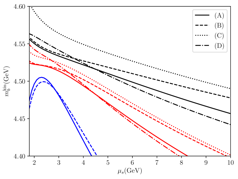
Figure 7: $\overline{m}_{b}^{\rm kin}$ computed from $\overline{m}_{b}(\mu_{s})$ using one-, two- and three-loop (blue, red, black) accuracy as a function of $\mu_{s}$. At each loop-order, four lines are shown, one for each of schemes (A) – (D).

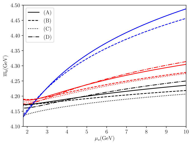
Figure 8: $\overline{m}_{b}(\overline{m}_{b})$ computed from $m^{\rm kin}$ using one-, two- and three-loop (blue, red, black) accuracy as a function of $\mu_{s}$. At each loop-order, four lines are shown, one for each of the scheme (A) – (D).

Both in Fig. 7 and Fig. 8, we observe a flattening of the curves after including higher order corrections. If we restrict ourselves to values of $\mu_{s}\geq 3$ GeV, the three-loop curves varies by about 25 MeV and 50 MeV, respectively, which suggests an uncertainty of $\pm 13$ MeV and $\pm 25$ MeV. Note, however, that a stronger $\mu_{s}$ dependence is observed below 2 GeV.

There are several options to estimate of the theoretical uncertainty associated to the $\overline{m}_{b}$–$m_{b}^{\rm kin}$ conversion formula.

• We proceed as in Ref. [16] and use half of the three-loop correction as an estimate on the size of the unknown higher orders. This leads to an uncertainty of about 15 MeV (excluding scheme (C)). Note that the same criterion applied to the two-loop mass relation leads to an uncertainty of about 40 MeV. Thus, the three-loop term leads to a reduction of the uncertainty by about a factor of two.

• An estimate of higher order effects is also obtained by varying $\mu_{s}$. If we choose $3~{}\mbox{GeV}\leq\mu_{s}\leq 9$ GeV we obtain an uncertainty of $\pm\{17,13,18,24\}$ MeV for the four schemes (see also Fig. 7). The same prescription at order $\alpha_{s}^{2}$ leads to an uncertainty of $\pm\{33,25,27,39\}$ MeV.

• An optimistic uncertainty estimate could be based on the four-loop large-$\beta_{0}$ approximation computed in Section 6. In that case we obtain 9 MeV for the missing four-loop term.

We recommend to use option 1.

Finally, we present simple formulae which can be used to convert the scale-invariant bottom quark mass to the kinetic scheme or vice versa using the preferred input values for the mass and strong coupling constant. We find

$$\frac{\overline{m}_{b}(\overline{m}_{b})}{\mbox{MeV}}= \{4195,4189,4171,4195\}+\Delta_{\rm kin}\{18,18,18,18\}$$

$$-\Delta_{\alpha_{s}}\{7,7,8,7\}\pm\{20,18,25,19\}\,,$$

$$\frac{m_{b}^{\rm kin}}{\mbox{MeV}}= \{4520,4526,4547,4521\}+\Delta_{\overline{\rm MS}}\{18,18,18,18\}$$

$$+\Delta_{\alpha_{s}}\{8,8,10,8\}\pm\{15,13,20,15\}\,,$$ (82)

where the three numbers in the curly brackets refer to schemes (A), (B), (C) and (D), respectively. For the quantities $\Delta_{X}$ we have

$$\Delta_{\rm kin} = (m_{b}^{\rm kin}/\mbox{MeV}-4550)/20\,,$$

$$\Delta_{\overline{\rm MS}} = (\overline{m}_{b}(\overline{m}_{b})/\mbox{MeV}-4163)/16\,,$$

$$\Delta_{\alpha_{s}} = (\alpha_{s}-0.1179)/0.001\,.$$ (83)

All numerical results presented in this Section can be reproduced using the implementation in RunDec and CRunDec [20, 84] in the functions mKIN2mMS[...] and mMS2mKIN[...]. For more details concerning the arguments, we refer to the latest version which can be downloaded from [84].

8 Conclusions

The aim of this paper has been the computation of the three-loop corrections to the relation between the heavy quark masses defined in the kinetic and the $\overline{\rm MS}$ schemes.

We described in detail the methods employed for the calculation of the mass relation. In particular the application of the asymptotic expansion in the threshold limit and the computation of the master integrals. For the latter we provided explicit analytic results. Our strategy is in principle extendable to $\alpha_{s}^{4}$, if such precision will ever become necessary in the future. We furthermore discussed in detail finite charm quark mass effects for the bottom mass relations.

The numerical analysis of the $m^{\rm kin}$–$m^{\overline{\rm MS}}$ relation shows a good convergence of the perturbative series, both for charm and bottom quark. Altogether, charm quark mass effects to the bottom mass are small and do not destabilize the convergence property of the series. The mass relation is mainly sensitive to the number of massless quarks, while it is rather insensitive to charm which behaves as a heavy degree of freedom. The new correction terms at three loops reduce the uncertainty due to scheme conversion by about a factor two.

The extraction of $|V_{cb}|$ from inclusive semileptonic $B$ decays is founded upon the kinetic scheme for the heavy quark masses and the HQE parameters. Therefore, the work presented in this paper is pivotal for future precision determinations of $|V_{cb}|$ at Belle II.

Appendix A Perturbative contributions to HQET parameters

In this section we give the perturbative contributions to HQET parameters $\overline{\Lambda},\mu_{\pi}^{2},\rho_{D}$ and $r_{E}$ up to order $\alpha_{s}^{3}$. These expressions can be employed to renormalize their non-perturbative versions in the so-called kinetic scheme. The definitions of $\overline{\Lambda}|_{\rm pert}$ and $\mu_{\pi}^{2}|_{\rm pert}$ were given in Eq. (22). The HQET parameters $\rho_{D}$ and $r_{E}$ are defined as:

$$2M_{B}\rho_{D}^{3} =\bra{H_{\infty}}\bar{h}_{v}iD_{\perp\mu}(iv\cdot D)iD_{\perp}^{\mu}h_{v}\ket{H_{\infty}},$$

$$2M_{B}r_{E}^{4} =-\bra{H_{\infty}}\bar{h}_{v}iD_{\perp\mu}(iv\cdot D)^{2}iD_{\perp}^{\mu}h_{v}\ket{H_{\infty}}.$$ (84)

Their perturbative versions are given by the SV sum rules:

$$[\rho_{D}^{3}(\mu)]_{\rm pert} =\lim_{\vec{v}\to 0}\lim_{m_{b}\to\infty}\frac{3}{\vec{v}\,^{2}}\frac{\displaystyle\int_{0}^{\mu}\omega^{3}\,W(\omega,\vec{v}\,)\,{\rm d}\omega}{\displaystyle\int_{0}^{\mu}W(\omega,\vec{v}\,){\rm d}\omega}\,,$$

$$[r_{E}^{4}(\mu)]_{\rm pert} =\lim_{\vec{v}\to 0}\lim_{m_{b}\to\infty}\frac{3}{\vec{v}\,^{2}}\frac{\displaystyle\int_{0}^{\mu}\omega^{4}\,W(\omega,\vec{v}\,)\,{\rm d}\omega}{\displaystyle\int_{0}^{\mu}W(\omega,\vec{v}\,){\rm d}\omega}\,.$$ (85)

Up to $O(\alpha_{s}^{3})$, the HQET parameters are given by the following expressions:

$$\left[\overline{\Lambda}(\mu)\right]_{\text{pert}} = \frac{\alpha_{s}^{(n_{l})}}{\pi}C_{F}\,\mu\Biggl{\{}\frac{4}{3}+\frac{\alpha_{s}^{(n_{l})}}{\pi}\biggl{[}\frac{1}{27}C_{A}\bigl{(}215-6\pi^{2}-66l_{\mu}\bigr{)}-\frac{8}{27}n_{l}T_{F}\bigl{(}8-3l_{\mu}\bigr{)}\biggr{]}$$ (86)

$$+\left(\frac{\alpha_{s}^{(n_{l})}}{\pi}\right)^{2}\biggl{[}C_{A}n_{l}T_{F}\biggl{(}-\frac{19453}{486}+2\zeta_{3}+\frac{1654l_{\mu}}{81}-\frac{88l_{\mu}^{2}}{27}+\frac{8\pi^{2}}{81}\bigl{(}13-3l_{\mu}\bigr{)}\biggr{)}$$

$$+C_{A}^{2}\biggl{(}\frac{130867}{1944}+\frac{\pi^{4}}{18}-\frac{19}{2}\zeta_{3}-\frac{2518l_{\mu}}{81}+\frac{121l_{\mu}^{2}}{27}-\frac{\pi^{2}}{162}\bigl{(}511-132l_{\mu}\bigr{)}\biggr{)}$$

$$+n_{l}^{2}T_{F}^{2}\biggl{(}\frac{1292}{243}-\frac{8\pi^{2}}{81}-\frac{256l_{\mu}}{81}+\frac{16l_{\mu}^{2}}{27}\biggr{)}$$

$$-C_{F}n_{l}T_{F}\biggl{(}\frac{11}{4}-\frac{4\zeta_{3}}{3}-\frac{2l_{\mu}}{3}\biggr{)}\biggr{]}\Biggr{\}}\,,$$

$$\left[\mu_{\pi}^{2}(\mu)\right]_{\text{pert}} = \frac{\alpha_{s}^{(n_{l})}}{\pi}C_{F}\,\mu^{2}\Biggl{\{}1+\frac{\alpha_{s}^{(n_{l})}}{\pi}\biggl{[}\frac{1}{18}C_{A}\bigl{(}91-3\pi^{2}-33l_{\mu}\bigr{)}-\frac{1}{9}n_{l}T_{F}\bigl{(}13-6l_{\mu}\bigr{)}\biggr{]}$$ (87)

$$+\left(\frac{\alpha_{s}^{(n_{l})}}{\pi}\right)^{2}\biggl{[}C_{A}n_{l}T_{F}\biggl{(}\frac{3}{2}\zeta_{3}-\frac{13699}{648}+\frac{1}{27}\pi^{2}\bigl{(}23-6l_{\mu}\bigr{)}+\frac{695l_{\mu}}{54}-\frac{22l_{\mu}^{2}}{9}\biggr{)}$$

$$+C_{A}^{2}\biggl{(}\frac{96295}{2592}+\frac{\pi^{4}}{24}-\frac{57}{8}\zeta_{3}-\frac{2155l_{\mu}}{108}+\frac{121l_{\mu}^{2}}{36}-\frac{1}{216}\pi^{2}\bigl{(}445-132l_{\mu}\bigr{)}\biggr{)}$$

$$+C_{F}n_{l}T_{F}\biggl{(}-\frac{29}{16}+\zeta_{3}+\frac{l_{\mu}}{2}\biggr{)}+n_{l}^{2}T_{F}^{2}\biggl{(}\frac{209}{81}-\frac{2\pi^{2}}{27}-\frac{52l_{\mu}}{27}+\frac{4l_{\mu}^{2}}{9}\biggr{)}\biggr{]}\Biggr{\}}\,,$$

$$\left[\rho_{D}^{3}(\mu)\right]_{\text{pert}} = \frac{\alpha_{s}^{(n_{l})}}{\pi}C_{F}\mu^{3}\Biggl{\{}\frac{2}{3}+\frac{\alpha_{s}^{(n_{l})}}{\pi}\biggl{[}\frac{1}{18}C_{A}\bigl{(}57-2\pi^{2}-22l_{\mu}\bigr{)}-\frac{4}{9}n_{l}T_{F}\bigl{(}2-l_{\mu}\bigr{)}\biggr{]}$$

$$+\left(\frac{\alpha_{s}^{(n_{l})}}{\pi}\right)^{2}\biggl{[}C_{A}n_{l}T_{F}\biggl{(}\zeta_{3}-\frac{12133}{972}+\frac{217l_{\mu}}{27}-\frac{44l_{\mu}^{2}}{27}+\frac{4}{81}\pi^{2}\bigl{(}11-3l_{\mu}\bigr{)}\biggr{)}$$

$$+C_{A}^{2}\biggl{(}\frac{86707}{3888}+\frac{\pi^{4}}{36}-\frac{19}{4}\zeta_{3}-\frac{113l_{\mu}}{9}+\frac{121l_{\mu}^{2}}{54}-\frac{1}{108}\pi^{2}\bigl{(}141-44l_{\mu}\bigr{)}\biggr{)}$$

$$+C_{F}n_{l}T_{F}\biggl{(}\frac{1}{72}\bigl{(}48\zeta_{3}-83\bigr{)}+\frac{l_{\mu}}{3}\biggr{)}+n_{l}^{2}T_{F}^{2}\biggl{(}\frac{358}{243}-\frac{4\pi^{2}}{81}-\frac{32l_{\mu}}{27}+\frac{8l_{\mu}^{2}}{27}\biggr{)}\biggr{]}\Biggr{\}}\,,$$

$$\left[r_{E}^{4}(\mu)\right]_{\text{pert}} = \frac{\alpha_{s}^{(n_{l})}}{\pi}C_{F}\mu^{4}\Biggl{\{}\frac{1}{2}+\frac{\alpha_{s}^{(n_{l})}}{\pi}\biggl{[}\frac{C_{A}}{144}\bigl{(}331-12\pi^{2}-132l_{\mu}\bigr{)}-\frac{1}{36}n_{l}T_{F}\bigl{(}23-12l_{\mu}\bigr{)}\biggr{]}$$ (89)

$$+\left(\frac{\alpha_{s}^{(n_{l})}}{\pi}\right)^{2}\biggl{[}C_{A}n_{l}T_{F}\biggl{(}\frac{3}{4}\zeta_{3}-\frac{1427}{162}+\frac{1}{108}\pi^{2}\big{(}43-12l_{\mu}\big{)}+\frac{629l_{\mu}}{108}-\frac{11l_{\mu}^{2}}{9}\biggr{)}$$

$$+C_{A}^{2}\biggl{(}\frac{20569}{1296}+\frac{\pi^{4}}{48}-\frac{57}{16}\zeta_{3}-\frac{3947l_{\mu}}{432}+\frac{121l_{\mu}^{2}}{72}-\frac{1}{108}\pi^{2}\bigl{(}103-33l_{\mu}\bigr{)}\biggr{)}$$

$$+C_{F}n_{l}T_{F}\biggl{(}-\frac{27}{32}+\frac{\zeta_{3}}{2}+\frac{l_{\mu}}{4}\biggr{)}+n_{l}^{2}T_{F}^{2}\biggl{(}\frac{331}{324}-\frac{\pi^{2}}{27}-\frac{23l_{\mu}}{27}+\frac{2l_{\mu}^{2}}{9}\biggr{)}\biggr{]}\Biggr{\}}\,,$$

with $l_{\mu}=\ln(2\mu/\mu_{s})$. Note that we chose to parametrize the relations in terms of $\alpha_{s}^{(n_{l})}(\mu_{s})$ since all dependence on heavy quark masses decouples. The analytic expressions from this appendix can be downloaded from [57].

Appendix B Calculation of $I_{7}^{3l}$

In this Appendix we describe the calculation of the master integral

$${I_{7}^{3l}}=\int\frac{{\rm d}^{d}\vec{v}}{(2\pi)^{3d}}\frac{1}{[-k_{1}^{2}][-k_{2}^{2}][-(k_{1}-k_{3})^{2}][-(k_{2}-k_{3})^{2}][-2k_{1}.p_{1}+y][-2k_{2}.p_{1}+y]}$$

$$\times\frac{1}{[-2k_{3}.p_{1}+y]}\,,$$ (90)

with $p_{1}^{2}=m^{2}$. We compute $I_{7}^{3l}$ including the terms of order $\epsilon$. Since we know that the integral scales uniformly as $y^{3d-11}m^{8-3d}$ we can set $y=m=1$.

The direct evaluation through Mellin-Barnes integrals and subsequent summation was not successful, since we encounter quite complicated threefold infinite sums already for the $\epsilon^{0}$ part. We thus follow the idea to introduce another scale $x$ into the problem and solve the associated differential equations. The boundary conditions may be fixed in the limit $x\to 0$ and $I_{7}$ can be extracted from the limit $x\to 1$.

We look at the auxiliary integral

$${\hat{I}_{12}}=\int\frac{{\rm d}^{d}\vec{v}}{(2\pi)^{3d}}\frac{1}{[-k_{1}^{2}][-k_{2}^{2}][-(k_{1}-k_{3})^{2}][-(k_{2}-k_{3})^{2}][-2k_{1}.p_{1}+1][{-2k_{2}.p_{1}}+x]}$$

$$\times\frac{1}{[-2{k_{3}.p_{1}}+x]}\,,$$ (91)

with $p_{1}^{2}=1$. Using LiteRed it is straightforward to find a closed system of differential equations for this family. The master integrals we encounter are

$$\hat{I}_{1} =\int\frac{{\rm d}^{d}\vec{v}}{(2\pi)^{3d}}\frac{1}{[-k_{2}^{2}][-(k_{1}-k_{3})^{2}][-(k_{2}-k_{3})^{2}][-2k_{1}.p_{1}+1]},$$

$$\hat{I}_{2} =\int\frac{{\rm d}^{d}\vec{v}}{(2\pi)^{3d}}\frac{1}{[-k_{1}^{2}][-(k_{1}-k_{3})^{2}][-(k_{2}-k_{3})^{2}][-2k_{2}.p_{1}+x]},$$

$$\hat{I}_{3} =\int\frac{{\rm d}^{d}\vec{v}}{(2\pi)^{3d}}\frac{1}{[-k_{2}^{2}][-(k_{1}-k_{3})^{2}][-(k_{2}-k_{3})^{2}][-2k_{1}.p_{1}+1][-2k_{3}.p_{1}+x]},$$

$$\hat{I}_{4} =\int\frac{{\rm d}^{d}\vec{v}}{(2\pi)^{3d}}\frac{1}{[-k_{2}^{2}][-(k_{1}-k_{3})^{2}][-(k_{2}-k_{3})^{2}][-2k_{1}.p_{1}+1][-2k_{2}.p_{1}+x]},$$

$$\hat{I}_{5} =\int\frac{{\rm d}^{d}\vec{v}}{(2\pi)^{3d}}\frac{1}{[-k_{1}^{2}][-(k_{1}-k_{3})^{2}][-(k_{2}-k_{3})^{2}][-2k_{1}.p_{1}+1][-2k_{2}.p_{1}+x]},$$

$$\hat{I}_{6} =\int\frac{{\rm d}^{d}\vec{v}}{(2\pi)^{3d}}\frac{1}{[-k_{1}^{2}][-k_{2}^{2}][-(k_{2}-k_{3})^{2}][-2k_{1}.p_{1}+1][-2k_{3}.p_{1}+x]},$$

$$\hat{I}_{7} =\int\frac{{\rm d}^{d}\vec{v}}{(2\pi)^{3d}}\frac{1}{[-k_{1}^{2}][-k_{2}^{2}][-(k_{1}-k_{3})^{2}][-2k_{2}.p_{1}+x][-2k_{3}.p_{1}+x]},$$

$$\hat{I}_{8} =\int\frac{{\rm d}^{d}\vec{v}}{(2\pi)^{3d}}\frac{1}{[-k_{1}^{2}][-k_{2}^{2}][-(k_{1}-k_{3})^{2}][-(k_{2}-k_{3})^{2}][-2k_{3}.p_{1}+x]},$$

$$\hat{I}_{9} =\int\frac{{\rm d}^{d}\vec{v}}{(2\pi)^{3d}}\frac{1}{[-k_{1}^{2}][-k_{2}^{2}][-(k_{1}-k_{3})^{2}][-2k_{1}.p_{1}+1][-2k_{2}.p_{1}+x][-2k_{3}.p_{1}+x]},$$

$$\hat{I}_{10} =\int\frac{{\rm d}^{d}\vec{v}}{(2\pi)^{3d}}\frac{1}{[-k_{1}^{2}][-k_{2}^{2}][-(k_{1}-k_{3})^{2}][-(k_{2}-k_{3})^{2}][-2k_{1}.p_{1}+1][-2k_{3}.p_{1}+x]},$$

$$\hat{I}_{11} =\int\frac{{\rm d}^{d}\vec{v}}{(2\pi)^{3d}}\frac{1}{[-k_{1}^{2}][-k_{2}^{2}][-(k_{1}-k_{3})^{2}][-(k_{2}-k_{3})^{2}][-2k_{1}.p_{1}+1][-2k_{2}.p_{1}+x]},$$

$$\hat{I}_{12} =\int\frac{{\rm d}^{d}\vec{v}}{(2\pi)^{3d}}\frac{1}{[-k_{1}^{2}][-k_{2}^{2}][-(k_{1}-k_{3})^{2}][-(k_{2}-k_{3})^{2}][-2k_{1}.p_{1}+1][-2k_{2}.p_{1}+x]}$$

$$\mbox{}\hskip 250.00038pt\times\frac{1}{[-2k_{3}.p_{1}+x]},$$

$$\hat{I}_{13} =\int\frac{{\rm d}^{d}\vec{v}}{(2\pi)^{3d}}\frac{1}{[-k_{1}^{2}]^{2}[-k_{2}^{2}][-(k_{1}-k_{3})^{2}][-(k_{2}-k_{3})^{2}][-2k_{1}.p_{1}+1][-2k_{2}.p_{1}+x]}$$

$$\mbox{}\hskip 250.00038pt\times\frac{1}{[-2k_{3}.p_{1}+x]}\,.$$ (92)

Note that $I_{7}^{3l}=\hat{I}_{12}|_{x=1}$.

Most of them can be easily computed for general $d$ and $x$ and we find

$$\hat{I}_{1} =\Gamma^{3}(d/2-1)\Gamma(7-3d),$$

$$\hat{I}_{2} =x^{3d-7}\Gamma^{3}(d/2-1)\Gamma(7-3d),$$

$$\hat{I}_{3} =\frac{\Gamma^{3}(d/2-1)\Gamma(8-3d)}{3-d}{}_{2}F_{1}\left(1,8-3d,4-d;1-x\right),$$

$$\hat{I}_{4} =\frac{\Gamma^{3}(d/2-1)\Gamma(8-3d)}{5-2d}{}_{2}F_{1}\left(1,8-3d,6-2d;1-x\right),$$

$$\hat{I}_{5} =\frac{\Gamma^{3}(d/2-1)\Gamma(8-3d)}{5-2d}{}_{2}F_{1}\left(1,d-2,6-2d;1-x\right),$$

$$\hat{I}_{6} =x^{2d-5}\Gamma^{3}(d/2-1)\Gamma(3-d)\Gamma(5-2d),$$

$$\hat{I}_{7} =x^{3d-8}\Gamma^{3}(d/2-1)\Gamma(3-d)\Gamma(5-2d),$$

$$\hat{I}_{8} =x^{3d-9}\frac{\Gamma^{2}(2-d/2)\Gamma^{4}(d/2-1)\Gamma(3d/2-4)\Gamma(9-3d)}{\Gamma(4-d)\Gamma^{2}(d-2)},$$

$$\hat{I}_{9} =\frac{\Gamma^{3}(d/2-1)\Gamma^{2}(3-d)\Gamma(6-2d)}{\Gamma(4-d)}{}_{2}F_{1}\left(6-2d,3-d,4-d;1-x\right).$$ (93)

The $\epsilon$-expansion of the hypergeometric functions can be obtained using HypExp [85, 86] or EvaluateMultiSums [44]. The integrals $\hat{I}_{10}$ to $\hat{I}_{13}$ can be determined through differential equations with the following boundary conditions

$$\left.\hat{I}_{10}\right|_{x=0} =\left.I_{12}^{3l}\right|_{y=1,m=1},$$ (94)

$$\left.\hat{I}_{11}\right|_{x\to 0} =\frac{x}{12\epsilon^{3}}+\frac{1}{\epsilon^{2}}\Bigl{[}-\frac{1}{24}+x\Bigl{(}\frac{2}{3}-\frac{1}{4}\ln(x)\Bigr{)}\Bigr{]}+\frac{1}{\epsilon}\Bigl{[}-\frac{13}{24}+x\Bigl{(}\frac{10}{3}+\frac{7}{24}\zeta_{2}-2\ln(x)$$

$$+\frac{1}{4}\ln^{2}(x)\Bigr{)}\Bigr{]}-\frac{109}{24}-\frac{29}{16}\zeta_{2}+\epsilon\Bigl{[}-\frac{757}{24}-\frac{345}{16}\zeta_{2}+\frac{23}{24}\zeta_{3}+x\Bigl{(}\frac{100}{3}+17\zeta_{2}-2\zeta_{3}$$

$$-\frac{6847}{480}\zeta_{2}^{2}-\bigl{(}52+23\zeta_{2}-\frac{23}{4}\zeta_{3}\bigr{)}\ln(x)+\bigl{(}11+\frac{23}{8}\zeta_{2}\bigr{)}\ln^{2}(x)-\frac{4}{3}\ln^{3}(x)$$

$$+\frac{1}{12}\ln^{4}(x)\Bigr{)}\Bigr{]}+\epsilon^{2}\Bigl{[}-\frac{4777}{24}-\frac{2649}{16}\zeta_{2}+\frac{395}{24}\zeta_{3}-\frac{3279}{64}\zeta_{2}^{2}+x\Bigl{(}-\frac{16}{3}+\frac{85}{3}\zeta_{2}$$

$$+\frac{58}{3}\zeta_{3}-\frac{763}{12}\zeta_{2}^{2}+\frac{463}{24}\zeta_{2}\zeta_{3}+\frac{1187}{60}\zeta_{5}-\bigl{(}228+\frac{253}{2}\zeta_{2}-46\zeta_{3}+\frac{749}{32}\zeta_{2}^{2}\bigr{)}\ln(x)$$

$$+\bigl{(}52+23\zeta_{2}-\frac{23}{4}\zeta_{3}\bigr{)}\ln^{2}(x)-\bigl{(}\frac{22}{3}+\frac{23}{12}\zeta_{2}\bigr{)}\ln^{3}(x)+\frac{2}{3}\ln^{4}(x)-\frac{1}{30}\ln^{5}(x)\Bigr{)}\Bigr{]},$$ (95)

$$\left.\hat{I}_{12}\right|_{x=0} =\left.I_{14}^{3l}\right|_{y=1,m=1}.$$ (96)

Note that we need the initial value of $\hat{I}_{11}$ up to $\mathcal{O}(x)$, since the homogeneous solution of its associated differential equation vanishes at $x=0$. We have used a Mellin-Barnes representation to obtain the expansion in $x$. We do not need the limit $x=0$ of $\hat{I}_{13}$ since the master integrals $\hat{I}_{12}$ and $\hat{I}_{13}$ are not linearly independent in the limit $x\to 1$. We use this to express the integration constants of $\hat{I}_{13}$ through the ones for $\hat{I}_{12}$ in a later step. The differential equations have singular behaviour at $x=0$ and $x=1$, leading to harmonic polylogarithms.

Solving the differential equations for $\hat{I}_{10}$ and $\hat{I}_{11}$ is simple, since they only depend on already known master integrals. The differential equations for $\hat{I}_{12}$ and $\hat{I}_{13}$ form a coupled $2\times 2$-system, which we decouple into a second order differential equation for $\hat{I}_{12}$ using the Mathematica package OreSys [87]. The differential equations are solved using HarmonicSums [45]. The solution of $\hat{I}_{13}$ can be constructed from the solution of $\hat{I}_{12}$, its derivatives and already known master integrals. We then use the fact that $\hat{I}_{12}$ and $\hat{I}_{13}$ are not linearly independent at $x=1$ to fix one half of the integration constants introduced by solving the differential equation. The other half can be fixed from the $x=0$ limit of $\hat{I}_{12}$. Fixing the boundary values in this way and expanding the general solution for $x\to 1$ we finally obtain

$$I_{7}^{3l} =y^{3d-11}(m^{2})^{4-3d/2}\left.\hat{I}_{12}\right|_{x=1}$$

$$=y^{3d-11}(m^{2})^{4-3d/2}\Biggl{[}-\frac{\zeta_{2}}{3\epsilon^{2}}+\frac{1}{\epsilon}\Bigl{(}-\frac{8}{3}\zeta_{2}+\frac{1}{3}\zeta_{3}\Bigr{)}-\frac{52}{3}\zeta_{2}+\frac{8}{3}\zeta_{3}-\frac{49}{30}\zeta_{2}^{2}$$

$$+\epsilon\Bigl{(}-\frac{320}{3}\zeta_{2}+\frac{52}{3}\zeta_{3}-\frac{196}{15}\zeta_{2}^{2}-\frac{11}{6}\zeta_{2}\zeta_{3}-\frac{83}{3}\zeta_{5}\Bigr{)}\Biggr{]}.$$ (97)

Appendix C Auxiliary integrals

In this Section we present the formulae for auxiliary integrals useful for the direct integration of the three-loop master integrals. They are given by

$$J_{0}(y,n_{1},n_{2},n_{3})=$$

$$\int\frac{{\rm d}^{d}v}{(2\pi)^{d}}\frac{1}{(-v^{2})^{n_{1}}(-2p\cdot v)^{n_{2}}(-2p\cdot v+y)^{n_{3}}}$$

$$=(m^{2})^{n_{1}-d/2}y^{d-2n_{1}-n_{2}-n_{3}}\frac{\Gamma(d-2n_{1}-n_{2})\Gamma(d/2-n_{1})\Gamma(2n_{1}+n_{2}+n_{3}-d)}{\Gamma(n_{1})\Gamma(n_{3})\Gamma(d-2n_{1})}\,,$$

$$J_{1}(y_{2},y_{3};n_{1},n_{2},n_{3})=$$

$$\int\frac{{\rm d}^{d}v}{(2\pi)^{d}}\frac{1}{(-v^{2})^{n_{1}}(-2p\cdot v+y_{2})^{n_{2}}(-2p\cdot v+y_{3})^{n_{3}}}$$

$$= (m^{2})^{n_{1}-d/2}\frac{\Gamma(d/2-n_{1})}{\Gamma(n_{1})\Gamma(n_{2})\Gamma(n_{3})\Gamma(d-2n_{1})}\frac{1}{2\pi i}\int_{-i\infty}^{+i\infty}dw\,y_{2}^{w}\,y_{3}^{d-2n_{1}-n_{2}-n_{3}-w}$$

$$\times\Gamma(n_{2}+w)\Gamma(-w)\Gamma(d-2n_{1}-n_{2}-w)\Gamma(2n_{1}+n_{2}+n_{3}+w-d)\,,$$

$$J_{2}(p,q;n_{1},n_{2},n_{3})=$$ (98)

$$\int\frac{{\rm d}^{d}v}{(2\pi)^{d}}\frac{1}{(-v^{2})^{n_{1}}[-(v-q)^{2}]^{n_{2}}(-2p\cdot v)^{n_{3}}}$$

$$= \frac{1}{\Gamma(n_{1})\Gamma(n_{2})\Gamma(n_{3})\Gamma(d-n_{1}-n_{2}-n_{3})}$$

$$\times\frac{1}{2\pi i}\int_{-i\infty}^{+i\infty}dw\,(-q^{2})^{w}(-2p\cdot q)^{d-2n_{1}-2n_{2}-n_{3}-2w}(m^{2})^{w+n_{1}+n_{2}-d/2}$$

$$\times\Gamma(-w)\Gamma(d-2n_{1}-n_{2}-n_{3}-w)\Gamma(n_{1}+w)$$

$$\times\Gamma(d/2-n_{1}-n_{2}-w)\Gamma(2n_{1}+2n_{2}+n_{3}+2w-d)\,.$$

References

- [1] M. Beneke and V. M. Braun, Nucl. Phys. B 426 (1994) 301 [hep-ph/9402364].
- [2] I. I. Y. Bigi, M. A. Shifman, N. G. Uraltsev and A. I. Vainshtein, Phys. Rev. D 50 (1994) 2234 [hep-ph/9402360].
- [3] M. Beneke, Phys. Lett. B 344 (1995) 341 [hep-ph/9408380].
- [4] P. Marquard, A. V. Smirnov, V. A. Smirnov and M. Steinhauser, Phys. Rev. Lett. 114 (2015) no.14, 142002 [arXiv:1502.01030 [hep-ph]].
- [5] P. Marquard, A. V. Smirnov, V. A. Smirnov, M. Steinhauser and D. Wellmann, Phys. Rev. D 94 (2016) no.7, 074025 [arXiv:1606.06754 [hep-ph]].
- [6] K. G. Chetyrkin, J. H. Kühn, A. Maier, P. Maierhofer, P. Marquard, M. Steinhauser and C. Sturm, [arXiv:1710.04249 [hep-ph]].
- [7] M. Beneke, Phys. Lett. B 434 (1998) 115 [hep-ph/9804241].
- [8] A. H. Hoang, Z. Ligeti and A. V. Manohar, Phys. Rev. D 59 (1999), 074017 [arXiv:hep-ph/9811239 [hep-ph]].
- [9] A. H. Hoang, Z. Ligeti and A. V. Manohar, Phys. Rev. Lett. 82 (1999), 277-280 [arXiv:hep-ph/9809423 [hep-ph]].
- [10] A. Hoang and T. Teubner, Phys. Rev. D 60 (1999), 114027 [arXiv:hep-ph/9904468 [hep-ph]].
- [11] A. Pineda, JHEP 06, 022 (2001) [arXiv:hep-ph/0105008 [hep-ph]].
- [12] A. H. Hoang, A. Jain, I. Scimemi and I. W. Stewart, Phys. Rev. Lett. 101 (2008), 151602 [arXiv:0803.4214 [hep-ph]].
- [13] A. H. Hoang, A. Jain, C. Lepenik, V. Mateu, M. Preisser, I. Scimemi and I. W. Stewart, JHEP 04 (2018), 003 [arXiv:1704.01580 [hep-ph]].
- [14] I. I. Bigi, M. A. Shifman, N. Uraltsev and A. I. Vainshtein, Phys. Rev. D 56 (1997), 4017-4030 [arXiv:hep-ph/9704245 [hep-ph]].
- [15] A. Czarnecki, K. Melnikov and N. Uraltsev, Phys. Rev. Lett. 80 (1998) 3189 [hep-ph/9708372].
- [16] M. Fael, K. Schönwald and M. Steinhauser, Phys. Rev. Lett. 125 (2020) no.5, 052003 [arXiv:2005.06487 [hep-ph]].
- [17] M. Beneke and V. A. Smirnov, Nucl. Phys. B 522 (1998) 321 [hep-ph/9711391].
- [18] V. A. Smirnov, Springer Tracts Mod. Phys. 250 (2012) 1.
- [19] I. I. Y. Bigi, M. A. Shifman, N. G. Uraltsev and A. I. Vainshtein, Phys. Rev. D 52 (1995) 196 [hep-ph/9405410].
- [20] F. Herren and M. Steinhauser, Comput. Phys. Commun. 224 (2018), 333-345 [arXiv:1703.03751 [hep-ph]].
- [21] P. Gambino, JHEP 09 (2011), 055 [arXiv:1107.3100 [hep-ph]].
- [22] J. Chay, H. Georgi and B. Grinstein, Phys. Lett. B 247 (1990), 399-405.
- [23] I. I. Bigi, M. A. Shifman, N. Uraltsev and A. I. Vainshtein, Phys. Rev. Lett. 71 (1993), 496-499 [arXiv:hep-ph/9304225 [hep-ph]].
- [24] A. V. Manohar and M. B. Wise, Phys. Rev. D 49 (1994), 1310-1329 [arXiv:hep-ph/9308246 [hep-ph]].
- [25] T. Mannel, Phys. Rev. D 50 (1994), 428-441 [arXiv:hep-ph/9403249 [hep-ph]].
- [26] A. V. Manohar and M. B. Wise, Camb. Monogr. Part. Phys. Nucl. Phys. Cosmol. 10 (2000), 1-191
- [27] M. A. Shifman and M. Voloshin, Sov. J. Nucl. Phys. 47 (1988), 511 ITEP-87-64.
- [28] N. Isgur, D. Scora, B. Grinstein and M. B. Wise, Phys. Rev. D 39 (1989), 799-818
- [29] N. Isgur and M. B. Wise, Phys. Lett. B 237 (1990), 527-530
- [30] K. G. Chetyrkin and M. Steinhauser, Nucl. Phys. B 573 (2000) 617 [hep-ph/9911434].
- [31] P. Marquard, A. V. Smirnov, V. A. Smirnov and M. Steinhauser, Phys. Rev. D 97 (2018) no.5, 054032 [arXiv:1801.08292 [hep-ph]].
- [32] K. Melnikov and T. v. Ritbergen, Phys. Lett. B 482 (2000) 99 [hep-ph/9912391].
- [33] P. Marquard, L. Mihaila, J. H. Piclum and M. Steinhauser, Nucl. Phys. B 773 (2007) 1 [hep-ph/0702185].
- [34] M. Fael, K. Schönwald and M. Steinhauser, JHEP 10 (2020), 087 [arXiv:2008.01102 [hep-ph]].
- [35] A. Pak and A. Smirnov, Eur. Phys. J. C 71 (2011), 1626 [arXiv:1011.4863 [hep-ph]].
- [36] R. N. Lee, A. V. Smirnov, V. A. Smirnov and M. Steinhauser, JHEP 1805 (2018) 187 [arXiv:1804.07310 [hep-ph]].
- [37] J. Blümlein, P. Marquard and N. Rana, Phys. Rev. D 99 (2019) no.1, 016013 [arXiv:1810.08943 [hep-ph]].
- [38] J. Davies, F. Herren, G. Mishima and M. Steinhauser, JHEP 05 (2019), 157 [arXiv:1904.11998 [hep-ph]].
- [39] F. Herren, “Precision Calculations for Higgs Boson Physics at the LHC - Four-Loop Corrections to Gluon-Fusion Processes and Higgs Boson Pair-Production at NNLO,”, PhD thesis, KIT, 2020.
- [40] R. N. Lee, arXiv:1212.2685 [hep-ph]; R. N. Lee, J. Phys. Conf. Ser. 523 (2014) 012059 [arXiv:1310.1145 [hep-ph]].
- [41] B. Ruijl, T. Ueda and J. Vermaseren, [arXiv:1707.06453 [hep-ph]].
- [42] A. V. Smirnov and F. S. Chuharev, arXiv:1901.07808 [hep-ph].
- [43] C. Schneider, Sém. Lothar. Combin. 56 (2007) 1, article B56b; C. Schneider, in: Computer Algebra in Quantum Field Theory: Integration, Summation and Special Functions Texts and Monographs in Symbolic Computation eds. C. Schneider and J. Blümlein (Springer, Wien, 2013) 325 arXiv:1304.4134 [cs.SC].
- [44] J. Ablinger, J. Blümlein, S. Klein and C. Schneider, Nucl. Phys. Proc. Suppl. 205-206 (2010) 110 [arXiv:1006.4797 [math-ph]]; J. Blümlein, A. Hasselhuhn and C. Schneider, PoS (RADCOR 2011) 032 [arXiv:1202.4303 [math-ph]]; C. Schneider, J. Phys. Conf. Ser. 523 (2014) 012037 [arXiv:1310.0160 [cs.SC]].
- [45] J. Vermaseren, Int. J. Mod. Phys. A 14 (1999), 2037-2076 [arXiv:hep-ph/9806280 [hep-ph]]; E. Remiddi and J. Vermaseren, Int. J. Mod. Phys. A 15 (2000), 725-754 [arXiv:hep-ph/9905237 [hep-ph]]; J. Blümlein, Comput. Phys. Commun. 180 (2009), 2218-2249 [arXiv:0901.3106 [hep-ph]]; J. Ablinger, Diploma Thesis, J. Kepler University Linz, 2009, arXiv:1011.1176 [math-ph]; J. Ablinger, J. Blümlein and C. Schneider, J. Math. Phys. 52 (2011) 102301 [arXiv:1105.6063 [math-ph]]; J. Ablinger, J. Blümlein and C. Schneider, J. Math. Phys. 54 (2013), 082301 [arXiv:1302.0378 [math-ph]]; J. Ablinger, Ph.D. Thesis, J. Kepler University Linz, 2012, arXiv:1305.0687 [math-ph]; J. Ablinger, J. Blümlein and C. Schneider, J. Phys. Conf. Ser. 523 (2014), 012060 [arXiv:1310.5645 [math-ph]]; J. Ablinger, J. Blümlein, C. Raab and C. Schneider, J. Math. Phys. 55 (2014), 112301 [arXiv:1407.1822 [hep-th]]; J. Ablinger, PoS LL2014 (2014), 019 [arXiv:1407.6180 [cs.SC]]; J. Ablinger, [arXiv:1606.02845 [cs.SC]]; J. Ablinger, PoS RADCOR2017 (2017), 069 [arXiv:1801.01039 [cs.SC]]; J. Ablinger, PoS LL2018 (2018), 063; J. Ablinger, [arXiv:1902.11001 [math.CO]].
- [46] M. Czakon, Comput. Phys. Commun. 175 (2006), 559-571 [arXiv:hep-ph/0511200 [hep-ph]].
- [47] A. V. Smirnov and V. A. Smirnov, Eur. Phys. J. C 62 (2009), 445-449 [arXiv:0901.0386 [hep-ph]].
- [48] H.R.P. Ferguson and D.H. Bailey, RNR Technical Report, RNR-91-032; H.R.P. Ferguson, D.H. Bailey and S. Arno, NASA Technical Report, NAS-96-005.
- [49] Fredrik Johansson and others. mpmath: a Python library for arbitrary-precision floating-point arithmetic (version 1.1.0), December 2018, http://mpmath.org/.
- [50] A. V. Smirnov, Comput. Phys. Commun. 204 (2016), 189-199 [arXiv:1511.03614 [hep-ph]].
- [51] M. Fael, K. Schönwald, M. Steinhauser, in preparation.
- [52] A. Kotikov, Phys. Lett. B 254 (1991), 158-164
- [53] T. Gehrmann and E. Remiddi, Nucl. Phys. B 580 (2000), 485-518 [arXiv:hep-ph/9912329 [hep-ph]].
- [54] J. M. Henn, Phys. Rev. Lett. 110 (2013), 251601 [arXiv:1304.1806 [hep-th]].
- [55] D. J. Broadhurst, J. Fleischer and O. Tarasov, Z. Phys. C 60 (1993), 287-302 [arXiv:hep-ph/9304303 [hep-ph]].
- [56] F. A. Berends, A. I. Davydychev and N. Ussyukina, Phys. Lett. B 426 (1998), 95-104 [arXiv:hep-ph/9712209 [hep-ph]].
-
[57]
https://www.ttp.kit.edu/preprints/2020/ttp20-040/. - [58] S. Bekavac, A. G. Grozin, D. Seidel and V. A. Smirnov, Nucl. Phys. B 819 (2009), 183-200 [arXiv:0903.4760 [hep-ph]].
- [59] D. J. Broadhurst, N. Gray and K. Schilcher, Z. Phys. C 52 (1991) 111.
- [60] S. Bekavac, A. Grozin, D. Seidel and M. Steinhauser, JHEP 10 (2007), 006 [arXiv:0708.1729 [hep-ph]].
- [61] A. I. Davydychev and A. Grozin, Phys. Rev. D 59 (1999), 054023 [arXiv:hep-ph/9809589 [hep-ph]].
- [62] K. Melnikov and T. van Ritbergen, Nucl. Phys. B 591 (2000) 515 [hep-ph/0005131].
- [63] N. Gray, D. J. Broadhurst, W. Grafe and K. Schilcher, Z. Phys. C 48 (1990) 673.
- [64] D. J. Broadhurst, Z. Phys. C 54 (1992) 599.
- [65] K. G. Chetyrkin, B. A. Kniehl and M. Steinhauser, Nucl. Phys. B 510 (1998), 61-87 [arXiv:hep-ph/9708255 [hep-ph]].
- [66] A. G. Grozin, M. Höschele, J. Hoff, M. Steinhauser, JHEP 09 (2011), 066 [arXiv:1107.5970 [hep-ph]].
- [67] K. G. Chetyrkin and M. Steinhauser, Phys. Rev. Lett. 83 (1999) 4001 [hep-ph/9907509].
- [68] S. J. Brodsky, G. Lepage and P. B. Mackenzie, Phys. Rev. D 28 (1983), 228
- [69] D. J. Broadhurst and A. Grozin, Phys. Rev. D 52 (1995), 4082-4098 [arXiv:hep-ph/9410240 [hep-ph]].
- [70] M. Beneke and V. M. Braun, Phys. Lett. B 348 (1995), 513-520 [arXiv:hep-ph/9411229 [hep-ph]].
- [71] R. Lee, P. Marquard, A. V. Smirnov, V. A. Smirnov and M. Steinhauser, JHEP 03 (2013), 162 [arXiv:1301.6481 [hep-ph]].
- [72] M. Tanabashi et al. [Particle Data Group], Phys. Rev. D 98 (2018) no.3, 030001
- [73] K. Chetyrkin, J. Kühn, A. Maier, P. Maierhofer, P. Marquard, M. Steinhauser and C. Sturm, Phys. Rev. D 80 (2009), 074010 [arXiv:0907.2110 [hep-ph]].
- [74] P. Gambino and C. Schwanda, Phys. Rev. D 89 (2014) no.1, 014022 [arXiv:1307.4551 [hep-ph]].
- [75] P. Gambino and J. F. Kamenik, Nucl. Phys. B 840 (2010), 424-437 [arXiv:1004.0114 [hep-ph]].
- [76] P. Baikov, K. Chetyrkin and J. Kühn, JHEP 10 (2014), 076 [arXiv:1402.6611 [hep-ph]].
- [77] T. Luthe, A. Maier, P. Marquard and Y. Schroder, JHEP 01 (2017), 081 [arXiv:1612.05512 [hep-ph]].
- [78] P. Baikov, K. Chetyrkin and J. Kühn, JHEP 04 (2017), 119 [arXiv:1702.01458 [hep-ph]].
- [79] P. A. Baikov, K. G. Chetyrkin and J. H. Kühn, Phys. Rev. Lett. 118 (2017) no.8, 082002 [arXiv:1606.08659 [hep-ph]].
- [80] F. Herzog, B. Ruijl, T. Ueda, J. A. M. Vermaseren and A. Vogt, JHEP 1702 (2017) 090 [arXiv:1701.01404 [hep-ph]].
- [81] T. Luthe, A. Maier, P. Marquard and Y. Schroder, JHEP 1710 (2017) 166 [arXiv:1709.07718 [hep-ph]].
- [82] K. Chetyrkin, G. Falcioni, F. Herzog and J. Vermaseren, JHEP 10 (2017), 179 [arXiv:1709.08541 [hep-ph]].
- [83] D. Benson, I. I. Bigi, T. Mannel and N. Uraltsev, Nucl. Phys. B 665 (2003), 367-401 [arXiv:hep-ph/0302262 [hep-ph]].
- [84] https://www.ttp.kit.edu/preprints/2017/ttp17-011
- [85] T. Huber and D. Maitre, Comput. Phys. Commun. 175 (2006), 122-144 [arXiv:hep-ph/0507094 [hep-ph]].
- [86] T. Huber and D. Maitre, Comput. Phys. Commun. 178 (2008), 755-776 [arXiv:0708.2443 [hep-ph]].
- [87] S. Gerhold, Uncoupling Systems of Linear Ore Operator Equations, Diploma Thesis, RISC, J. Kepler University, Linz, February 2002.