Inconsistencies arising from the coupling of galaxy formation sub-grid models to Pressure-Smoothed Particle Hydrodynamics

Abstract

Smoothed Particle Hydrodynamics (SPH) is a Lagrangian method for solving the fluid equations that is commonplace in astrophysics, prized for its natural adaptivity and stability. The choice of variable to smooth in SPH has been the topic of contention, with smoothed pressure (P-SPH) being introduced to reduce errors at contact discontinuities relative to smoothed density schemes. Smoothed pressure schemes produce excellent results in isolated hydrodynamics tests; in more complex situations however, especially when coupling to the ‘sub-grid’ physics and multiple time-stepping used in many state-of-the-art astrophysics simulations, these schemes produce large force errors that can easily evade detection as they do not manifest as energy non-conservation. Here two scenarios are evaluated: the injection of energy into the fluid (common for stellar feedback) and radiative cooling. In the former scenario, force and energy conservation errors manifest (of the same order as the injected energy), and in the latter large force errors that change rapidly over a few timesteps lead to instability in the fluid (of the same order as the energy lost to cooling). Potential ways to remedy these issues are explored with solutions generally leading to large increases in computational cost. Schemes using a Density-based formulation do not create these instabilities and as such it is recommended that they are preferred over Pressure-based solutions when combined with an energy diffusion term to reduce errors at contact discontinuities.

1 Introduction

Over the past three decades, the inclusion of hydrodynamics in (cosmological) galaxy formation simulations has become commonplace (Hernquist & Katz, 1989; Evrard et al., 1994; Springel & Hernquist, 2002; Springel, 2005; Dolag et al., 2009). One of the first hydrodynamics methods to be used in such simulations was Smoothed Particle Hydrodynamics (SPH, Gingold & Monaghan, 1977; Monaghan, 1992). SPH is prized for its adaptivity, conservation properties, and stability and is still used in state-of-the-art simulations by many groups today (Schaye et al., 2015; Teklu et al., 2015; McCarthy et al., 2017; Tremmel et al., 2017; Cui et al., 2019; Steinwandel et al., 2020); see Vogelsberger et al. (2020) for a recent overview of cosmological simulations.

As the SPH method has developed, two key issues have arisen. The first, a consequence of the non-diffusive nature of the SPH equations, was that the method was unable to capture shocks. This was resolved by the addition of a diffusive ‘artificial viscosity’ term (Monaghan & Gingold, 1983). This added diffusivity is only required in shocks, and so many schemes include particle-carried switches for the viscosity (Morris & Monaghan, 1997; Cullen & Dehnen, 2010) to prevent unnecessary conversion between kinetic and thermal energy in e.g. shearing flows. The second, artificial surface tension appearing in contact discontinuities (e.g. Agertz et al., 2007), has led to the development of several mitigation procedures. One possible solution is artificial conductivity (also known as energy diffusion) to smooth out the discontinuity (e.g. Price, 2008; Read & Hayfield, 2012; Rosswog, 2019); this method applies an extra equation of motion to the thermodynamic variable to transfer energy between particles. The alternative solution, generally favoured in the cosmology community, is to reconstruct a smooth pressure field (Ritchie & Thomas, 2001; Saitoh & Makino, 2013; Hopkins, 2013). This smooth pressure field allows for a gradual transition pressure between hot and cold fluids, suppressing any variation in the thermodynamic variable at scales smaller than the resolution limit. This can be beneficial in fluids where there is a high degree of mixing between phases, such as in gas flowing into galactic haloes (e.g. Tumlinson et al., 2017; Stern et al., 2019).

Cosmological simulations typically include so-called ‘sub-grid’ physics that aims to represent underlying physics that is below the (mass) resolution limit (which is usually around $10^{3-7}\;{\rm M}_{\odot}{}$; Vogelsberger et al., 2014; Schaye et al., 2015; Hopkins et al., 2018; Marinacci et al., 2019; Davé et al., 2019). This is commonplace in many fields, and is essential in galaxy formation to reproduce many of the observed properties of galaxies. One key piece of sub-grid physics is star formation, which occurs on mass scales smaller than a solar mass. Cold, dense, gas is required to enable stars to form; to reach these temperatures and densities radiative cooling (which occurs on atomic scales) must be included in a sub-grid fashion. Finally, when these stars have reached the end of their life some will produce supernovae explosions, which are modelled using sub-grid ‘feedback’ schemes (such a sub-grid scheme is chosen for many reasons, including but not limited to limited resolution and the ’overcooling problem’; see Navarro & White, 1993; Dalla Vecchia & Schaye, 2012, and references for more information). Each of these processes has an impact on the hydrodynamics solver which must be carefully examined. Here we employ a simple galaxy formation model including implicit cooling and energetic feedback, based on the EAGLE galaxy formation model (Schaye et al., 2015), to understand how the inclusion of such a model may affect simulations employing Density- or Pressure-based SPH differently. We note, however, that the results obtained in the following sections are applicable to all kinds of galaxy formation models, including those that instead use instantaneous or ‘operator-split’ cooling.

The rest of this paper is organised as follows: In §2 the SPH method is described, along with the Density- and Pressure-based schemes; in §3 the basics of a galaxy formation model are discussed in more detail; in §4 issues relating to injection of energy into Pressure-based schemes are explored; in §5 the SPH equations of motion are discussed; in §6 the time-integration schemes used in cosmological simulations are presented and issues with sub-grid cooling are explored, and in §7 it is concluded that while Pressure-SPH schemes can introduce significant errors it is possible in some cases to use measures (albeit computationally expensive ones) to remedy them. Because of this added expense it is suggested that a Density-based scheme is preferred, with an energy diffusion term used to mediate contact discontinuities.

2 Smoothed Particle Hydrodynamics

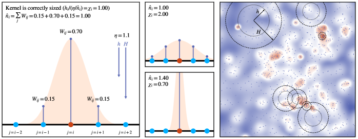
Figure 1: The three leftmost panels show the consequences of choosing a correct (large, left), too large (top right), and too small (bottom right) smoothing length (for $\eta=1.1$) in 1D on a set of particles with an expected density $\hat{n}=1$. This is quantified through both the density, $\hat{n}$, for the central particle $i$, and the ratio between the chosen smoothing length $h_{i}$ and the expected smoothing length given by $\eta/\hat{n}_{i}$, parametrised as $\chi_{i}$. $\chi_{i}$ is a well behaved function of the smoothing length, and finding the root of $\chi_{i}-1$ is a reliable way to choose the value of $h_{i}$ that corresponds to a given choice of $\eta$. Note how the density is only erroneous in the case with a smoothing length that is too small (bottom panel); the larger smoothing length (top panel) produces the correct density but would be less computationally efficient and inconsistent with the chosen value of $\eta$. The rightmost panel shows a 2D case with a random particle distribution, with the background colour map showing the low (blue) to high (white and then red) density regions and the associated variation in smoothing length. Here, for selected particles, the smoothing length $h$ and kernel cut-off radius $H$ are shown with dotted and dashed lines respectively. In particular, note how the higher density regions show smaller smoothing lengths such that Equation 1 is respected.

Parameter Name	Symbol	Symbolic Units	Description
Number of dimensions	$n_{D}$	None	Number of spatial dimensions (1-3)
Particle position	$\mathbf{r}_{i}$	[l]	Cartesian vector position of particles
Inter-particle separation	$r_{ij}=|\mathbf{r}_{i}-\mathbf{r}_{j}|$	[l]	Euclidean distance between two particles $i$ and $j$
Smoothing length	$h_{i}$	[l]	Particle-carried smoothing length corresponding to FWHM of gaussian
Number density	$\hat{n}_{i}$	[l]${}^{-n_{D}}$	Local particle number density, i.e. the local density of particles
Kernel	$W_{ij}=W(r_{ij},h_{i})$	[l]${}^{-n_{D}}$	Value of the kernel at the distance between particles $i$ and $j$
Eta	$\eta$	None	Ratio of local inter-particle separation to smoothing length
Kernel support ratio	$\gamma_{K}$	None	Ratio between cut-off radius of the kernel and smoothing length; kernel-dependent
Ratio of specific heats	$\gamma$	None	The ratio of specific heats for the ideal gas, here $\gamma=C_{P}/C_{V}=5/3$
Cut-off radius	$H_{i}=\gamma_{K}h_{i}$	[l]	Maximal radius at which the kernel takes a non-zero value
Density	$\hat{\rho}_{i}$	[m][l]${}^{-n_{D}}$	Local mass density, here defined at the position of particle $i$
Particle mass	$m_{i}$	[m]	The mass of a particle, here the mass of particle $i$
Internal energy	$u_{i}$	[l]2[t]-2	Internal energy per unit mass of particle $i$
Entropy	$A_{i}$	[m]1-γ[l]3γ-1[t]-2	Entropy per unit mass of particle $i$
Pressure	$P_{i}$ or $\hat{P}_{i}$	[m][l]-1[t]-2	Pressure of the field, either at particle positions (left) or smoothed (right)
Sound-speed	$c_{{\rm s},i}$	[l][t]-1	Speed of sound at the position of particle $i$
Weighted density	$\bar{\rho}_{i}$	[m][l]-3	Smoothed pressure-weighted density, i.e. $\hat{P}_{i}/((\gamma-1)u_{i})$
Particle velocity	$\mathbf{v}_{i}$	[l][t]-1	Cartesian vector velocity of the particle $i$
h-factor	$f_{ij}$	None	Correction factor for variable smoothing lengths (between particles $i$ and $j$)

Table 1: Table of symbols used in the rest of the paper. Symbols are defined, along with their units (in terms of unit mass [m], unit length [l], and unit time [t]) here.

SPH is a Lagrangian method that uses particles to discretise the fluid. To find the equation of motion for the system, and hence integrate a fluid in time, the forces acting on each particle are required. In a fluid, these forces are determined by the local pressure field acting on the particles. The ultimate goal of the SPH method, then, is to find the pressure gradient associated with a set of discretised particles; once this is obtained finding the equations of motion is a relatively simple task. The reader is referred to the first few pages of the review by Price (2012) for more information on the fundamentals of the SPH method.

Before continuing, it is important to separate the two types of quantities present in SPH. The first, particle carried properties (denoted as symbols with an index corresponding to their particle, e.g. $m_{i}$ is the mass of particle $i$), are valid only at the positions of particles in the system and include variables such as mass. The second, field properties (denoted as symbols with a hat, and with a corresponding index if they are evaluated at particle positions, such as $\hat{\rho}_{i}$, the density at the position of particle $i$), are valid at all points in the computational domain, and generally are volumetric quantities. These field properties are built out of particle-carried properties by convolving them with the smoothing kernel.

The smoothing kernel is a weighting function of two parameters, inter-particle separation ($|\mathbf{r}_{i}-\mathbf{r}_{j}|=r_{ij}$) and smoothing length $h_{i}$, with a shape similar to a Gaussian with a full-width half maximum of $\sqrt{2\ln 2}h_{i}$. The smoothing lengths of particles are chosen such that, for each particle, the following equation is satisfied:

$$\hat{n}_{i}=\sum_{{\rm All~{}particles}~{}j}W(r_{ij},h_{i})=\left(\frac{\eta}{h_{i}}\right)^{n_{D}},$$ (1)

where $\hat{n}_{i}$ is the local number density, $n_{D}$ the number of spatial dimensions, and the kernel $W(r_{ij},h_{i})$ (henceforth written as $W_{ij}$) has the same dimensions as number density, typically being composed of a dimensionless weighting function $w_{ij}=w(r_{ij}/h_{i})$ such that $W_{ij}\propto w_{ij}h_{i}^{-n_{D}}$. $\eta$ is a dimensionless parameter that determines how smooth the field reconstruction should be (effectively setting the spatial resolution), with larger values leading to kernels that encompass more particles and typically takes values around $\eta\approx 1.2$. An important distinction is the difference between the smoothing length, $h_{i}$, related to the full-width half-maximum (FWHM) of the Gaussian that the kernel approximates, and the kernel cut-off radius $H_{i}$. This cut-off radius is parametrised as $H_{i}=\gamma_{K}h_{i}$, with $\gamma_{K}$ a kernel-dependent quantity taking values around $1.5-2.5$, such that $H_{i}$ gives the maximum value of $r_{ij}$ at which the kernel will be non-zero. We note that Table 1 shows all symbols used regularly throughout this paper and encourage readers to refer to it when necessary.

An example kernel (the cubic spline kernel, see Dehnen & Aly, 2012, for significantly more information on kernels) is shown in Fig. 1, with three choices for the smoothing length that satisfy Equation 1: one that is too large; one that is ‘just right’ for the given choice of $\eta$, and one that is too small. The choice to satisfy both equations is not strictly equivalent to ensuring that the kernel encompasses a fixed number of neighbouring particles; note how the edges of the kernel in the left panel do not coincide with a particle, even despite their uniform spacing.

To evaluate the mass density of the system, at the particle positions, the kernel is again used to re-evaluate the above equation now including the particle masses such that the density

$$\hat{\rho}_{i}=\sum_{j}m_{j}W_{ij}$$ (2)

is the sum over the kernel contributions and neighbouring masses $m_{j}$ that may differ between particles. Note that this summation includes the self-contribution from the particle $i$, $m_{i}W(0,h_{i})$.

Typically in SPH, the particle-carried property of either internal energy $u_{i}$, or entropy $A_{i}$ (per unit mass) is chosen to encode the thermal properties of the particle. These are related to each other, and the particle-carried pressure, through the ideal gas equation of state

$$P_{i}=(\gamma-1)u_{i}\hat{\rho}_{i}=A_{i}\hat{\rho}^{\gamma},$$ (3)

with the ratio of specific heats $\gamma=C_{P}/C_{V}=5/3$ for the fluids usually considered in cosmological hydrodynamics models.

Alternatively, it is possible to construct a smooth pressure field that is evaluated at the particle positions such that

$$\hat{P}_{i}=\sum_{j}(\gamma-1)m_{j}u_{j}W_{ij}=\left(\sum_{j}m_{j}A_{j}^{1/\gamma}W_{ij}\right)^{\gamma},$$ (4)

directly includes the particle-carried thermal quantities of the neighbours into the definition of the pressure.

The differences between SPH models that use the particle pressures evaluated through the equation of state and smoothed density (i.e. those that use Equations 2 and 3), known as Density SPH, and those that use the smooth pressures (i.e. those that use Equation 4), known as Pressure SPH, is the central topic of this paper. Frequently, the SPH scheme is also referred to by its choice of thermodynamic variable, internal energy or entropy, as Density-Energy (Density-Entropy) or Pressure-Energy (Pressure-Entropy).

SPH schemes are usually implemented as a fixed number of ‘loops over neighbours’ (often just called loops). For a basic scheme like the ones presented above, two loops are usually used. The first loop, frequently called the ‘density’ loop, goes over all neighbours $j$ of all particles $i$ to calculate their SPH density (Equation 2) or smooth pressure (Equation 4). The second loop, often called the ‘force’ loop, evaluates the equation of motion for each particle $i$ through the use of the pre-calculated smoothed quantities of all neighbours $j$. Each loop is computationally expensive, and so schemes that require extra loops are generally unfavourable unless they provide a significant benefit. State-of-the-art schemes typically use three loops, inserting a ‘gradient’ loop between the ‘density’ and ‘force’ loops to calculate either improved gradient estimators (Rosswog, 2019) or coefficients for artificial viscosity and diffusion schemes (Price, 2008; Cullen & Dehnen, 2010).

3 A simple galaxy formation model

The discussion that follows requires an understanding of two pieces of a galaxy formation model: energy injection into the fluid and energy removal from the fluid. These are used to model the processes of supernovae and AGN feedback, and radiative cooling respectively. The results presented here are not necessarily tied to the model used, and are applicable to a wide range of current galaxy formation models that use Pressure-based SPH schemes. Here we use a simplified version of the EAGLE galaxy formation model as an instructive example, as this used Pressure-Entropy SPH for its hydrodynamics model in Schaye et al. (2015) and associated works (of particular note is Schaller et al., 2015, that discusses the effects of the choice of numerical SPH scheme on galaxy properties).

3.1 Cooling

The following equation is solved implicitly for each particle separately:

$$u(t+\Delta t)=u(t)+\frac{\mathrm{d}u}{\mathrm{d}t}(t)\Delta t,$$ (5)

where $\mathrm{d}u/\mathrm{d}t$ being the ‘cooling rate’ calculated from the underlying atomic processes with the resulting final internal energy being transformed into an average rate of change of internal energy as a function of time over the step,

$$\bar{\frac{\mathrm{d}u}{\mathrm{d}t}}=\frac{u(t+\Delta t)-u(t_{i})}{\Delta t}.$$ (6)

After this occurs, this rate is limited in some circumstances (see Schaye et al., 2015, for more detail) that are not relevant to the discussion here. This average ‘cooling rate’ is then applied as either an addition to the $\mathrm{d}u/\mathrm{d}t$ or $\mathrm{d}A/\mathrm{d}t$ from the hydrodynamics scheme for each particle depending on the variable that the scheme tracks.

3.2 Energy Injection Feedback

A common, simple, feedback model is implemented as heating particles by a constant temperature jump. It is possible to implement different types of feedback with this method, all being represented with a separate change in temperature $\Delta T$. For supernovae feedback, $\Delta T_{\rm SNII}=10^{7.5}$ K, and for AGN $\Delta T_{\rm AGN}=10^{8.5}$ K (in EAGLE). The change in temperature does not actually ensure that the particle has this temperature once the feedback has taken place, however; the amount of energy corresponding to heating a particle from 0 K to this temperature is added to the particle. This ensures that even in cases where the particle is hotter than the heating temperature energy is still injected.

To apply feedback to a given particle, this change in temperature must be converted to a change in internal energy. This is performed by using a linear relationship between temperature and internal energy to find the internal energy that corresponds to a temperature of $\Delta T$, and adding this additional energy onto the internal energy of the particle.

4 Energy injection in Pressure-Entropy

In cosmology codes it is typical to use the particle-carried entropy as the thermodynamic variable rather than the internal energy. This custom originated because in many codes (of particular note here is Gadget; Springel, 2005) the choice of co-ordinates in a space co-moving with expansion due to dark energy is such that the entropy variable is cosmology-less, i.e. it is the same in physical and co-moving space. Entropy is also conserved under adiabatic expansion, meaning that fewer equations of motion are required. This makes it convenient from an implementation point of view to track entropy rather than internal energy. However, at the level of the equation of motion, this makes no difference, as this is essentially just a choice of co-ordinate system.

This naturally leads the Pressure-Entropy variant (i.e. as opposed to Pressure-Energy) of the Pressure-based schemes to be frequently chosen; here the main smoothed quantity is pressure, with entropy being the thermodynamic variable.

The Pressure-Entropy and Pressure-Energy scheme perform equally well on hydrodynamics tests (see Hopkins (2013) for a collection), but when coupling to sub-grid physics there are some key differences.

For an entropy-based scheme, energy injection naturally leads to a conversion between the requested energy input and an increase in entropy for the relevant particle. Considering a Density-Entropy scheme to begin with (e.g. Springel & Hernquist, 2002), with only a smooth density $\hat{\rho}$,

$$P_{i}=(\gamma-1)u_{i}\hat{\rho}_{i},$$ (7)

with $P$ the pressure from the equation of state, $\gamma$ the ratio of specific heats, and $u_{i}$ the particle energy per unit mass. In addition, the expression for the pressure as a function of the entropy $A_{i}$,

$$P_{i}=A_{i}\hat{\rho}^{\gamma}.$$ (8)

Given that these should give the same thermodynamic pressure, the pressure variable can be eliminated to give

$$u_{i}=\frac{A_{i}\hat{\rho}^{\gamma-1}}{\gamma-1}$$ (9)

and as these variables are independent for a change in energy $\Delta u$ the change in entropy can be written

$$\Delta A_{i}=(\gamma-1)\frac{\Delta u_{i}}{\hat{\rho}^{\gamma-1}}.$$ (10)

For any energy based scheme (either Density-Energy or Pressure-Energy), it is possible to directly modify the internal energy per unit mass $u$ of a particle, and this directly corresponds to the same change in total energy of the field. This is clearly also true here too for the Density-Entropy scheme. Then, the sum of all energies (converted from entropies in the Density-Entropy case) in the box will be the original value plus the injected energy, without the requirement for an extra loop over neighbours.

Now considering Pressure-Entropy, the smoothed pressure shown in Equation 4 at a particle depends on a smoothed entropy over all of its neighbours. To connect the internal energy and entropy of a particle again the equation of state can be used by introducing a new variable, the weighted density $\bar{\rho}$,

$$\hat{P}_{i}=(\gamma-1)u_{i}\bar{\rho}_{i}=A_{i}\bar{\rho}_{i}^{\gamma}$$ (11)

now being rearranged to eliminate the weighted density $\bar{\rho}$ such that

$$A_{i}(u_{i})=\hat{P}_{i}^{1-\gamma}(\gamma-1)u_{i}^{\gamma},$$ (12)

$$u_{i}(A_{i})=\frac{A_{i}^{1/\gamma}\hat{P}^{1-1/\gamma}}{\gamma-1}.$$ (13)

To inject energy into the field by explicitly heating a single particle $i$ in any entropy-based scheme the key is to find $\Delta A_{i}$ for a given $\Delta u_{i}$. In a pressure-based scheme this is problematic, as (converting Equation 12 to a set of differences),

$$\Delta A=\hat{P}_{i}(A_{i})^{1-\gamma}(\gamma-1)(u_{i}+\Delta u)^{\gamma}-A_{i},$$ (14)

to find this difference requires conversion via the smoothed pressure which directly depends on the value of $A_{i}$. This also occurs for the particles that neighbour $i$, meaning that there will be a non-zero change in the energy $u_{j}$ that they report. Hence, this means that simply solving a linear equation for $\Delta A(\Delta u)$ is not enough; whilst this can be calculated, the true change in energy of the whole field will not be $\Delta u$ (as it was in Density-Entropy) because of the changing pressures of the neighbours. When attempting to inject energy it is vital that these contributions to the total field energy are considered. To correctly account for these changes, we must turn to an iterative solution.

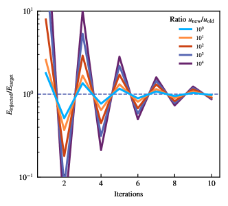
Figure 2: Energy injection as a function of iterations of the neighbour loop-based algorithm in Pressure-Entropy. Different coloured lines show ratios of injected energy to the original energy of the chosen particle, increasing in steps of 10. This algorithm allows for the correct energy to be injected into each particle after around 10 iterations, however more complex convergence criteria could be incorporated. A better estimate of the change in the smoothed pressure $\hat{P}$ could also significantly improve convergence.

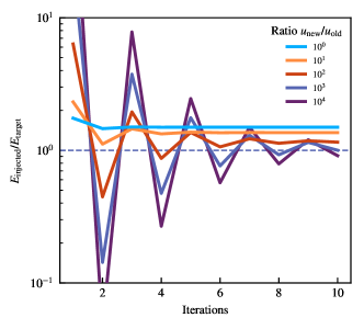
Figure 3: The same as Fig. 2, however this time using an approximate algorithm that only updates the self-contribution of the heated particle. This version of the algorithm shows non-convergent behaviour at low energy injection values, but is significantly computationally cheaper than solutions that require neighbour loops during the iteration procedure.

A simple algorithm for injecting energy $\Delta u$ in this case would be as follows:

1. Calculate the total energy of all particles that neighbour the one that will have energy injected, $u_{{\rm field},i}=\sum_{j}u(A_{j},\hat{P}_{j})$.

2. Find a target energy for the field, $u_{{\rm field},t}=u_{{\rm field},i}+\Delta u$.

3. While the energy of the field $u_{{\rm field}}=\sum_{j}u(A_{j},\hat{P}_{j})$ is outside of the bounds of the target energy:

   1. Calculate $A_{\rm inject}=A(u_{{\rm field},t}-u_{{\rm field}},\hat{P})$ for the particle that will have energy injected (i.e. apply Equation 14 assuming that $\hat{P}_{i}$ does not change).

   2. Add on $A_{\rm inject}$ to the entropy of the chosen particle.

   3. Re-calculate the smoothed pressures for all neighbouring particles.

   4. Re-calculate the energy of the field $u_{{\rm field}}$ (i.e. go to item iii above).

The results of this process, for various injection energies, are shown in Fig. 2. After around 10 iterations, the requested injection of energy is reached. This process is valid only for working on a single particle at a time, however, and as such would be non-trivial to parallelise without the use of locks on particles that were currently being modified. Suddenly changing the energy of a neighbouring particle while this process was being performed would destroy the convergent behaviour that is demonstrated in Fig. 2.

Even without locks, this algorithm is computationally expensive, with many thousands of operations required to change a single variable. Re-calculating the smoothed pressure (step c) for every particle multiple times per step, is generally infeasible as it would require many thousands of operations per particle per step. An ideal algorithm would not require neighbour loops; only updating the self contribution for the heated particle:

1. Calculate the total energy of the particle that will have the energy injected, $u_{i,{\rm initial}}=u(A_{i},\hat{P}_{i})$.

2. Find a target energy for the particle, $u_{i,{\rm target}}=u_{i,{\rm initial}}+\Delta u$.

3. While the energy of the particle $u_{i}=u(A_{i},\hat{P}_{i})$ is outside of the bounds of the target energy (tolerance here is $10^{-6}$, and is rarely reached) and the number of iterations is below the maximum (10):

   1. Calculate $A_{\rm inject}=A(u_{i,t}-u_{i},\hat{P})$ for the particle that will have the energy injected.

   2. Add on $A_{\rm inject}$ to the entropy of that particle.

   3. Update the self contribution to the smoothed pressure for the injection particle by $\hat{P}_{i,{\rm new}}=\left[\hat{P}_{i,{\rm old}}^{1/\gamma}+(A_{\rm new}^{1/\gamma}-A_{\rm old}^{1/\gamma})W_{0}\right]^{\gamma}$ with $W_{0}=W(0,h_{i})$ the kernel self-contribution term.

   4. Re-calculate the energy of the particle $u_{i}=u(A_{i},\hat{P}_{i})$ using the new entropy and energy of that particle (i.e. go to iii above).

The implementation of the faster procedure is shown in Fig. 3. This simple algorithm leads to significantly higher than expected energy injection for low (relative) energy injection events. For the case of the requested energy injection being the same as the initial particle energy, over 50% too much energy is injected into the field. For events that inject more entropy into particle $i$, the value $A_{i}^{1/\gamma}W_{ij}$ for all neighbouring kernels becomes the leading component of the smoothed pressure field. This allows the pressure field to be dominated by this one particle, meaning that changes in $A_{i}^{1/\gamma}$ represent linear changes in the pressures of neighbouring particles, and hence allowing the simple methodology to correctly predict the changes in the global internal energy field.

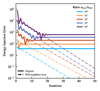
Figure 4: Comparison between the simple energy injection procedure (Fig. 3, solid lines) against the method including a neighbour loop each iteration (Fig. 2, dashed lines) for various energy injection values. The vertical axis here shows the energy offset from the true requested energy (in absolute arbitrary code units). The neighbour loop approach allows for the injected energy error to decrease with each iteration, where the simple procedure has a fixed (injection dependent) energy error that is reached rapidly at low values of energy injection where the entropies of neighbouring particles remain dominant.

The error in the computationally cheaper injection method is directly compared against the neighbour loop procedure from Fig. 2 in Fig. 4. The extra energy injected per event is clear here; the method using a full neighbour loop each iteration manages to reduce the error each iteration, with the non neighbour loop method showing a fixed offset after a few iterations. This also shows that the energy injection error grows as the amount injected grows, despite this becoming a lower relative fraction of the requested energy.

It is unclear exactly how much these errors impact the results of a full cosmological run. For the case of supernovae following Dalla Vecchia & Schaye (2012), which has a factor of $u_{\rm new}/u_{\rm old}\approx 10^{4}$ this should not represent a significant overinjection (the energy converges within 10 iterations to around a percent or so). For feedback pathways that inject a relatively smaller amount of energy (for instance SNIa, AGN events on particles that have been recently heated, events on particles in haloes with a high virial temperature, or schemes that inject using smaller steps of energy or into multiple particles simultaneously) there will be a significantly larger amount of energy injected than initially expected. This uncontrolled energy injection is clearly undesirable.

4.1 A Different Injection Procedure

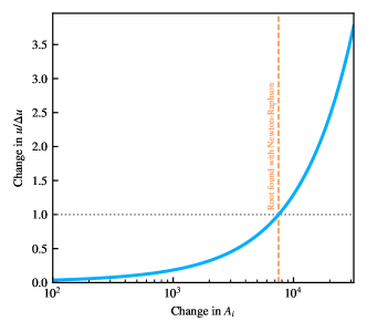
Figure 5: The blue line shows the dependence of change in field energy $u$ as a function of the change in the entropy $A_{i}$ of a single particle, for a requested change in energy $\Delta u$. This change in energy $\Delta u$ corresponds to a heating event from $10^{3.5}$ K to $10^{7.5}$ K (a factor of $10^{4}$ in $u$), which corresponds to a typical energetic supernovae feedback event. The orange dashed line shows the predicted change in $A_{i}$ for this change $\Delta u$ from the iterative solution (using the Newton-Raphson method) of Equation 18.

Pressure-Entropy based schemes have been shown to be unable to inject the correct amount of energy using a simple algorithm based on updating only a single particle (i.e. without neighbour loops), however it is possible to perform this task exactly within a single step by using an iterative solver to find the change in entropy $\Delta A$.

To inject a set amount of energy $\Delta u$ the total energy of the field $u_{\rm tot}$ must be modified by changing the properties of particle $i$ (with neighbouring particles $j$), with

$$u_{\rm tot}=\frac{1}{\gamma-1}\left(\sum_{j}m_{j}A_{j}^{1/\gamma}W_{ij}\right)^{\gamma-1}.$$ (15)

This can be re-arranged to extract components specifically dependent on the injection particle $i$,

$$u_{\rm tot}=\frac{1}{1-\gamma}\sum_{j\neq i} A_{j}^{1/\gamma}\left({p}_{j,i}+m_{i}A_{i}^{1/\gamma}W_{ij}\right)^{\gamma-1}$$

$$+ A_{i}^{1/\gamma}\left({p}_{i,i}+m_{i}A_{i}^{1/\gamma}W_{ii}\right)^{\gamma-1},$$ (16)

with

$${p}_{a,b}=\hat{P}_{b}-m_{b}A^{1/\gamma}_{b}W_{ab}.$$ (17)

Finally, now considering a change in energy $\Delta u$ as a function of the change in entropy for particle $i$, $\Delta A$,

$$\Delta u=\frac{1}{1-\gamma}\sum_{j\neq i} A_{j}^{1/\gamma}\left({p}_{j,i}+m_{i}(A_{i}+\Delta A)^{1/\gamma}W_{ij}\right)^{\gamma-1}$$

$$+ (A_{i}+\Delta A)^{1/\gamma}\left({p}_{i,i}+m_{i}(A_{i}+\Delta A)^{1/\gamma}W_{ii}\right)^{\gamma-1}$$

$$- u_{\rm tot},$$ (18)

which can be solved iteratively using, for example, the Newton-Raphson method. This method converges very well in just a few steps to calculate the change in entropy $\Delta A$ as demonstrated in Fig. 5. In practice, this method would require two loops over the neighbours of particle $i$ per injection event. In the first loop, the values of $p_{j,i}$ and $W_{ij}$ would be calculated and stored, with the iterative solver then used to find the appropriate value of $\Delta A$. These changes would then need to be back-propagated to the neighbouring particles, as their smoothed pressures $\hat{P}_{j}$ will have changed significantly, reversing the procedure in Equation 17.

Such a scheme could potentially make a Pressure-Entropy based SPH method viable for a model that uses energy injection. This procedure requires tens of thousands of operations per thermal injection event, however, and as such would require significant effort to implement efficiently.

This also highlights a possible issue with Pressure-Energy based SPH schemes, as even in this case, where it is much simpler to make changes to the global energy field, changes to the internal energy of a particle must be back-propagated to neighbours to ensure that the pressure and internal energy fields remain consistent. These errors also compound, should more than one particle in a kernel be heated without the back-propagation of changes.

5 Equations of Motion

So far only static fields have been under consideration; before moving on to discussing the effects of sub-grid cooling on pressure-based schemes, the dynamics part of SPH must be considered. Below only two equations of motion are described, the one corresponding to Density-Energy, and the equation of motion for Pressure-Energy SPH. For a more expanded derivation of the following from a Lagrangian and the first law of Thermodynamics see Hopkins (2013), or the Swift simulation code theory documentation.

5.1 Density-Energy

For Density-Energy the smoothed quantity of interest is the smoothed mass density (Equation 2). This leads to a corresponding equation of motion for velocity of

$$\frac{\mathrm{d}\mathbf{v}_{i}}{\mathrm{d}t}=-\sum_{j}m_{j} \left[f_{i}\frac{P_{i}}{\hat{\rho}_{i}^{2}}\nabla W(r_{i\!j},h_{i})+f_{j}\frac{P_{j}}{\hat{\rho}_{j}^{2}}\nabla W(r_{ji},h_{j})\right],$$ (19)

with the $f_{i}$ here representing correction factors for interactions between particles with different smoothing lengths

$$f_{i}=\left(1+\frac{h_{i}}{n_{d}\hat{\rho}_{i}}\frac{\partial\hat{\rho}_{i}}{\partial h_{i}}\right)^{-1}.$$ (20)

This factor also enters into the equation of motion for the internal energy

$$\frac{\mathrm{d}u_{i}}{\mathrm{d}t}=\sum_{j}m_{j}f_{i}\frac{P_{i}}{\hat{\rho}_{i}^{2}}\mathbf{v}_{ij}\cdot\nabla W(r_{ij},h_{i}).$$ (21)

5.2 Pressure-Energy

For Pressure-Energy SPH, the thermodynamic quantity $u$ remains the same as for Density-Energy, but the smoothed pressure field $\hat{P}$ is introduced (see Equation 4). This is then used in the equation of motion for the particle velocities

$$\frac{\mathrm{d}\mathbf{v}_{i}}{\mathrm{d}t}=-\sum_{j}(\gamma-1)^{2}m_{j}u_{j}u_{i}\left[\frac{f_{ij}}{\hat{P}_{i}}\nabla W(r_{ij},h_{i})+\frac{f_{ji}}{\hat{P}_{j}}\nabla W(r_{ji},h_{j})\right].$$ (22)

with the $f_{ij}$ now depending on both particle $i$ and $j$

$$f_{ij}=1-\left[\frac{h_{i}}{n_{d}(\gamma-1)\hat{n}_{i}m_{j}u_{j}}\frac{\partial\hat{P}_{i}}{\partial h_{i}}\right]\left(1+\frac{h_{i}}{n_{d}\hat{n}_{i}}\frac{\partial\hat{n}_{i}}{\partial h_{i}}\right)^{-1},$$ (23)

with $\hat{n}$ the local particle number density (Equation 1). Again, this factor enters into the equation of motion for the internal energy

$$\frac{\mathrm{d}u_{i}}{\mathrm{d}t}=(\gamma-1)^{2}\sum_{j}m_{j}u_{i}u_{j}\frac{f_{ij}}{\hat{P}_{i}}\mathbf{v}_{ij}\cdot\nabla W_{ij}.$$ (24)

5.3 Choosing an Appropriate Time-Step

To integrate these forward in time, an appropriate time-step between the evaluation of these smoothed equations of motion must be chosen. SPH schemes typically use a modified version of the Courant–Friedrichs–Lewy (CFL, Courant et al., 1928) condition to determine this step length. The CFL condition takes the form of

$$\Delta t=C_{\rm CFL}\frac{H_{i}}{c_{\rm s}},$$ (25)

with $c_{\rm s}$ the local sound-speed, and $C_{\rm CFL}$ a constant that should be strictly less than 1.0, typically taking a value of 0.1-0.3. Computing this sound-speed is a simple affair in density-based SPH, with it being a particle-carried property that is a function solely of other particle carried properties,

$$c_{\rm s}=\sqrt{\gamma\frac{P}{\hat{\rho}}}=\sqrt{\gamma(\gamma-1)u}.$$ (26)

For pressure-based schemes this requires a little more thought. The same sound-speed can be used, but this is not representative of the variables that actually enter the equation of motion. To clarify this, first consider the equation of motion for Density-Energy (Equation 19) and re-write it in terms of the sound-speed,

$$\frac{\mathrm{d}\mathbf{v}_{i}}{\mathrm{d}t}\sim\frac{c_{{\rm s},i}^{2}}{\hat{\rho}_{i}}\nabla_{i}W_{ij},$$

and for Pressure-Energy (Equation 22)

$$\frac{\mathrm{d}\mathbf{v}_{i}}{\mathrm{d}t}\sim(\gamma-1)^{2}\frac{u_{i}u_{j}}{\hat{P}_{i}}\nabla_{i}W_{ij}.$$

From this it is reasonable to assume that the sound-speed, i.e. the speed at which information propagates in the system through pressure waves, is given by the expression

$$c_{\rm s}=(\gamma-1)u_{i}\sqrt{\gamma\frac{\hat{\rho}_{i}}{\hat{P}_{i}}}.$$ (27)

This expression is dimensionally consistent with a sound-speed, and includes the gas density information (through $\hat{\rho}$), traditionally used for sound-speeds, as well as including the extra information from the smoothed pressure $\hat{P}$. However, such a sound-speed leads to a considerably higher time-step in front of a shock wave (where the smoothed pressure is higher, but the smooth density is relatively constant), leading to time integration problems. Using

$$c_{\rm s}=\sqrt{\gamma\frac{\hat{P}_{i}}{\hat{\rho}_{i}}}$$ (28)

instead of Equation 27 leads to a sound-speed that does not represent the equation of motion as directly but does not lead to time-integration problems, and effectively represents a smoothed internal energy field. It is also possible to use the same sound-speed using the particle-carried internal energy directly above.

6 Time Integration

A typical astrophysics SPH code will use Leapfrog integration or a velocity-verlet scheme to integrate particles through time (see e.g. Hernquist & Katz, 1989; Springel, 2005; Borrow et al., 2018). This approach takes the accelerations, $\mathbf{a}_{i}=\mathrm{d}\mathbf{v}_{i}/\mathrm{d}t$, and the velocities, $\mathbf{v}_{i}=\mathrm{d}\mathbf{r}_{i}/\mathrm{d}t$ and solves the system for the positions $r_{i}(t)$ as a function of time. It is convenient to write the equations as follows (for each particle):

$$\mathbf{v}\left(t+\frac{\Delta t}{2}\right) =\mathbf{v}(t)+\frac{\Delta t}{2}\mathbf{a}(t),$$ (29)

$$\mathbf{r}\left(t+\Delta t\right) =\mathbf{r}(t)+\mathbf{v}\left(t+\frac{\Delta t}{2}\right)\Delta t,$$ (30)

$$\mathbf{v}\left(t+\Delta t\right) =\mathbf{v}\left(t+\frac{\Delta t}{2}\right)+\frac{\Delta t}{2}\mathbf{a}(t+\Delta t),$$ (31)

commonly referred to (in order) as a Kick-Drift-Kick scheme. Importantly, these equations must be solved for all variables of interest.

This leapfrog time-integration is prized for its second order accuracy (in $\Delta t$) despite only including first order operators, due to cancelling second order terms as well as its manifest conservation of energy (Hernquist & Katz, 1989).

6.1 Multiple Time-Stepping

As noted above, it is possible to find a reasonable time-step to evolve a given hydrodynamical system with using the CFL condition (Equation 25). This condition applies on a particle-by-particle basis, meaning that to evolve the whole system a method for combining these individual time-steps into a global mechanism must be devised. In less adaptive problems than those considered here (e.g. those with little dynamic range in smoothing length), it is reasonable to find the minimal time-step over all particles, and evolve the whole system with this time-step. This scenario is frequently referred to as ‘single-d$t$’.

For a cosmological simulation, however, the huge dynamic range in smoothing length (and hence time-step) amongst particles means that evolving the whole system with a single time-step would render most simulations infeasible (Borrow et al., 2018). Instead, each particle is evolved according to its own time-step (referred to as a multi-d$t$ simulation) using a so-called ‘time-step hierarchy’ as originally described in Hernquist & Katz (1989). This choice is common-place in astrophysics codes (Teyssier, 2002; Springel, 2005).

In some steps in a multi-d$t$ simulation only the particles on the very shortest time-steps are updated in a loop over their neighbours to re-calculate, for example, $\hat{\rho}$ (referred to as these particles being ‘active’). The rest of the particles are referred to as being ‘inactive’. As the inactive particles may interact with the active ones, their properties must be interpolated, or drifted, to the current time.

For particle-carried quantities, such as the internal energy $u$, a simple first-order equation is used,

$$u\left(t+\Delta t\right)=u+\frac{\mathrm{d}u}{\mathrm{d}t}\Delta t.$$ (32)

6.2 Drifting Smoothed Quantities

As a particle may experience many more drift steps than loops over neighbours (that are only performed for active particles), it is important to have drift operators ($\mathrm{d}\hat{x}/\mathrm{d}t$) for smoothed quantities $\hat{x}$ to interpolate their values between full time-steps. This is achieved through taking the time differential of smoothed quantities. Starting with the simplest, the smoothed number density,

$$\frac{\mathrm{d}\hat{n}_{i}}{\mathrm{d}t} =\sum_{j}\frac{\mathrm{d}W(r_{ij},h_{i})}{\mathrm{d}t},$$

$$=\sum_{j}\mathbf{v}_{ij}\cdot\nabla_{j}W(r_{ij},h_{i}).$$ (33)

Following this process through for the smoothed quantities of interest yields

$$\frac{\mathrm{d}\hat{\rho}_{i}}{\mathrm{d}t} =\sum_{j}m_{j}\mathbf{v}_{ij}\cdot\nabla_{j}W(r_{ij},h_{i}),$$ (34)

$$\frac{\mathrm{d}\hat{P}_{i}}{\mathrm{d}t} =(\gamma-1)\sum_{j}m_{j}\left(W_{ij}\frac{\mathrm{d}u_{j}}{\mathrm{d}t}+u_{j}\mathbf{v}_{ij}\cdot\nabla_{j}W_{ij}\right),$$ (35)

for the smoothed density and pressure respectively, with $W_{ij}=W(r_{ij},h_{i})$. In the smoothed density case, the pressure is re-calculated at each drift step from the now drifted internal energy and density using the equation of state.

The latter drift equation, due to its inclusion of $\mathrm{d}u_{j}/\mathrm{d}t$ (i.e. the rate of change of internal energy of all neighbours of particle $i$), presents several issues. This sum is difficult to compute in practice; it requires that all of the $\mathrm{d}u_{j}/\mathrm{d}t$ are set before a neighbour loop takes place. This would require an extra loop over neighbours after the ‘force’ loop, which has generally been considered computationally infeasible for a scheme that purports to be so cheap. In practice, the following is used to drift the smoothed pressure:

$$\frac{\mathrm{d}\hat{P}_{i}}{\mathrm{d}t}=\frac{\mathrm{d}\hat{\rho}_{i}}{\mathrm{d}t}\cdot\frac{\mathrm{d}u_{i}}{\mathrm{d}t}~{},$$ (36)

which clearly does not fully capture the expected behaviour of Equation 35 as it only includes the rate of change of the internal energy for particle $i$, discarding the contribution from neighbours.

Such behaviour becomes particularly problematic in cases where sub-grid cooling is used, where particles within a kernel may have both very large $\mathrm{d}u_{j}/\mathrm{d}t$ (where $(\mathrm{d}u_{j}/\mathrm{d}t)\Delta t$ is comparable to $u_{j}$), and $\mathrm{d}u_{j}/\mathrm{d}t$ that vary rapidly with time. Consider the case where an active particle cools rapidly from some temperature to the equilibrium temperature in one step (which occurs frequently in a typical cosmological simulation where no criterion on the time-step for $\mathrm{d}u/\mathrm{d}t$ is included to ensure the number of steps required to complete the calculation remains reasonable whilst employing implicit cooling). If this particle has a neighbour at the equilibrium temperature that is inactive, the pressure for the neighbouring particle will remain significantly (potentially orders of magnitude) higher than what is mandated by the local internal energy field, leading to force errors of a similar level.

To apply these drift operators to smoothed quantities, instead of using a linear drift as in Equation 32, the analytic solution to these first order differential equations is used. For a smooth quantity $\hat{x}$ it is drifted forwards in time using

$$\hat{x}(t+\Delta t)=\hat{x}(t)\cdot\exp\left(\frac{1}{\hat{x}}\frac{\mathrm{d}\hat{x}}{\mathrm{d}t}\right).$$ (37)

This also has the added benefit of preventing the smoothed quantities from becoming negative. For this to be accurate, it requires an accurate $\mathrm{d}\hat{x}/\mathrm{d}t$ term.

6.3 Impact of Drift Operators in multi-d$t$

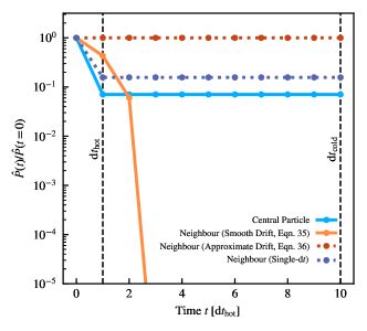
Figure 6: Smooth pressure as a function of time for different strategies in a uniform fluid of ‘cold’ particles, with one initially ‘hot’ particle with a temperature 100 times higher than the cold particles that cools to the ‘cold’ temperature in one time-step. The solid blue line shows the pressure of the central particle as a function of time (relative to its initial pressure). The dashed blue line shows the pressure of the closest ‘hot’ neighbour in a single-d$t$ scenario, i.e. the whole system is evolved with time-step d$t_{\rm hot}$. This shows the true answer for the pressure of the neighbour particle. The dotted red line shows the result of drifting the cold particle with Equation 36. As this particle has no cooling rate, and the fluid is stationary, the pressure does not change. The solid orange line shows the result of drifting using Equation 35. This rapidly leads to the particle having a pressure of zero, a highly undesirable result. Note that the orange line does not follow the dashed blue line in the first few steps due to different drifting schemes for smoothed and particle-carried quantities (Equation 32 and 37).

Whilst the true drift operator for $\hat{P}$ appears to be impractical from a computational perspective due to the requirement of another loop over neighbours, at first glance it appears that the use of this correct drift operator would remedy the issues with cooling. Unfortunately, in a multi-d$t$ simulation where active and in-active particles are mixed, this ‘correct’ operator can still lead to negative pressures when applied.

In Fig. 6 the different ways of drifting smooth pressure in a multi-d$t$ simulation are explored. In this highly idealised test, a cubic volume of uniform ‘cold’ fluid is considered. A single particle at the center is set to have a ‘hot’ temperature of 100 times higher than the background fluid, and is set to have a cooling rate that ensures that it cools to the ‘cold’ temperature within its first time-step. This scenario is similar to a hot $10^{6}$ K particle in the CGM cooling to join particles in the ISM at the $10^{4}$ K equilibrium temperature. The difference between the time-step of the hot and cold particles, implied by Equation 25, is a factor of 10 (when using the original definition of sound-speed, see Equation 26). Here the cold particle is drifted ten times to interact with its hot neighbour over a single time-step of its own. In practice, this scenario would evolve slightly differently, with the previously hot particle having its time-step re-set to d$t_{\rm cool}$ after it has cooled to the equilibrium temperature, but the nuances of the time-step hierarchy are ignored here for simplicity.

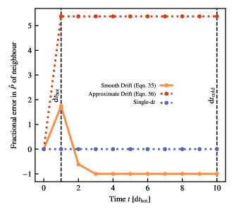
Figure 7: The same lines as Fig. 6, except now showing the ‘error’ as a function of time relative to the single-d$t$ case (blue dashed line) of the pressure $\hat{P}$ of the nearest neighbour to the ‘hot’ particle. Here the fractional error is defined as $\hat{P}(t)-\hat{P}_{\rm{single-d}t}/\hat{P}_{\rm{single-d}t}$. The orange line showing the drifting using Equation 35 shows that the pressure rapidly drops to zero after around four steps. The red dotted line (Equation 36) shows the offset in pressure that is maintained even after the central ‘hot’ particle cools.

The three drifting scenarios proceed very differently. In Fig. 7 the fractional errors relative to the single-d$t$ case are shown.

In the case of the drift using Equation 35, the pressure rapidly drops to zero. This is prevented from becoming negative thanks to the integration strategy that is employed (Equation 37); the rate of $\mathrm{d}\hat{P}/\mathrm{d}t$ is high enough to lead to negative pressures within a few drift steps should a simple linear integration strategy like that employed for the internal energy (Equation 32) be used. Because there is only a linear time integration (with a poorly chosen time-step for the equation to be evolved) method for a now non-linear problem (as there is a significant $\mathrm{d}^{2}u/\mathrm{d}t^{2}$ from changes in cooling rate) errors naturally manifest.

The drift operator using a combination of the local cooling rate and density time differential (Equation 36) is the safest, leading to pressures that are higher than expected; this does however come at the cost of larger relative errors in the pressure (500% increase v.s. 100% decrease; both of these are highly undesirable).

6.3.1 Limiting time-steps

One way to address the issues presented in Fig. 6 is to limit the time-steps between neighbouring particles. Such a ‘time-step limiter’ is common-place in galaxy formation simulations, as they are key to capturing the energy injected during feedback events (see e.g. Durier & Dalla Vecchia, 2012). In addition, the use of the ‘smoothed’ sound-speed (from Equation 28) ensures that the neighbouring particle has a time-step that is much closer to the time-step of the ‘hot’ particle than the sound-speed based solely on the internal energy of each particle alone. However, as Fig. 7 shows, even only after one intervening time-step (i.e. after $\mathrm{d}t_{\rm hot}$), there is a 50% to 500% error in the pressure of the neighbouring particle.

This error in the pressure of the neighbouring particle represents a poorly tracked non-conservation of energy. An incorrect relationship between the local internal energy and pressure field of the particles leads directly to force errors of the same magnitude. Because of the conservative and symmetric structure of the applied equations of motion, however, this does not lead to the total energy of the fluid changing over time (i.e. the sum of the kinetic and internal energy of the fluid remains constant), instead manifesting as unstable dynamics.

7 Conclusions

The Pressure-Energy and Pressure-Entropy schemes have been prized for their ability to capture contact discontinuities significantly better than their Density-based cousins due to their use of a directly smoothed pressure field (Hopkins, 2013). However, there are several disadvantages to using these schemes that have been presented:

• Injecting energy in a Pressure-Entropy based scheme requires the use of an iterative solver and many transformations between variables. This makes this scheme computationally expensive, and as such for this to be used in practice an efficient implementation is required. Approximate solutions do exist, but result in incorrect amounts of energy being injected into the field when particles are heated only by a small amount (typically by less than 100 times their own internal energy). This occurs even in the case where the fluid is evolved with a single, global, time-step, and is complicated even further by the inclusion of the multiple time-stepping scheme that is commonplace in cosmological simulations.

• In a Pressure-Energy based scheme, the injection of energy in a multi-d$t$ simulation requires either ‘waking up’ all of the neighbours of the affected particle (and forcing them to be active in the next time-step), or a loop over these neighbours to back-port changes to their pressure due to the changes in internal energy of the heated particle. This is a computationally expensive procedure, and is generally avoided in the practical use of these schemes. As such, while no explicit energy conservation errors manifest, there is an offset between the energy field represented by the particle distribution and the associated smooth pressure field in practical implementations.

• These issues also manifest themselves in cases where energy is removed from active particles, such as an ‘operator-splitting’ radiative cooling scheme where energy is directly removed from particles.

• Correctly ‘drifting’ the smoothed pressure of particles (as is required in a multi-d$t$ simulation) requires knowing the time differential of the smoothed pressure. To compute this, either an extra loop over neighbours is required for active particles, or an approximate solution based on the time differential of the density field and internal energy field is used. This approximate solution does not account for the changes taking place in the local internal energy field and as such does not correctly capture the evolution of the smoothed pressure.

• Even when using the ‘correct’ drift operator for the smoothed pressure significant pressure, and hence force, errors can occur when particles cool rapidly. This can be mitigated somewhat with time-step limiting techniques (either through the use of a time-step limiter like the one described in Durier & Dalla Vecchia (2012) or through a careful construction of a more representative sound-speed) but it is not possible to prevent errors on the same order as the relative energy difference between the cooling particle and its neighbours.

All of the above listed issues are symptomatic of one main flaw in these schemes; the SPH method assumes that the variables being smoothed over vary slowly during a single time-step. This is often true for the internal energy or particle entropy in idealised hydrodynamics tests, but in practical simulations with sub-grid radiative cooling (and energy injection) this leads to significant errors. These errors could be mitigated by using a different cooling model, where over a single time-step only small changes in the energies of particles could be made (i.e. by limiting the time-steps of particles to significantly less than their cooling time), however this would render most cosmological simulations impractical to complete due to the huge increase in the number of time-steps to finish the simulation that this would imply.

Thankfully, due to the explicit connection between internal energy and pressure in the Density-based SPH schemes, they do not suffer the same ills. They also smooth over the mass field, which either does not vary or generally varies very slowly (on much larger timescales than the local dynamical time). As such, the only recommendation that it is possible to make is to move away from Pressure-based schemes in favour of their Density-based cousins, solving the surface tension issues at contact discontinuities with artificial conduction instead of relying on the smoothed pressure field from Pressure-based schemes. It is worth noting that most modern implementations of the Pressure-based schemes already use an artificial conduction (also known as energy diffusion) term to resolve residual errors in fluid mixing problems Hu et al. (2014); Hopkins (2015). Of particular note is the lack of phase mixing (due to the non-diffusive nature of SPH) between hot and cold fluids, even in Pressure-SPH.

8 Acknowledgements

The authors would like to thank Joop Schaye and Claudio Dalla Vecchia for their helpful conversations. JB is supported by STFC studentship ST/R504725/1. MS is supported by the Netherlands Organisation for Scientific Research (NWO) through VENI grant 639.041.749. This work used the DiRAC@Durham facility managed by the Institute for Computational Cosmology on behalf of the STFC DiRAC HPC Facility (www.dirac.ac.uk). The equipment was funded by BEIS capital funding via STFC capital grants ST/K00042X/1, ST/P002293/1, ST/R002371/1 and ST/S002502/1, Durham University and STFC operations grant ST/R000832/1. DiRAC is part of the National e-Infrastructure.

8.1 Software Citations

This paper made use of the following software packages:

• python (van Rossum & Drake Jr, 1995), with the following libraries

  • numpy (Harris et al., 2020)

  • scipy (SciPy 1.0 Contributors et al., 2020)

  • matplotlib (Hunter, 2007)

  • numba (Lam et al., 2015)

  • swiftsimio (Borrow & Borrisov, 2020)

9 Data Availability

No new data were generated or analysed in support of this research. The figures in this paper were all produced from the equations described within, and all programs used to generate those figures are available in the GitHub repository at https://github.com/JBorrow/pressure-sph-paper-plots. They are also available in the online supplementary material accompanying this article.

References

- Agertz et al. (2007) Agertz O., et al., 2007, Monthly Notices of the Royal Astronomical Society, 380, 963
- Borrow & Borrisov (2020) Borrow J., Borrisov A., 2020, Journal of Open Source Software, 5, 2430
- Borrow et al. (2018) Borrow J., Bower R. G., Draper P. W., Gonnet P., Schaller M., 2018, Proceedings of the 13th SPHERIC International Workshop, Galway, Ireland, June 26-28 2018, pp 44–51
- Courant et al. (1928) Courant R., Friedrichs K., Lewy H., 1928, Mathematische Annalen, 100, 32
- Cui et al. (2019) Cui W., et al., 2019, Monthly Notices of the Royal Astronomical Society, 485, 2367
- Cullen & Dehnen (2010) Cullen L., Dehnen W., 2010, Monthly Notices of the Royal Astronomical Society, 408, 669
- Dalla Vecchia & Schaye (2012) Dalla Vecchia C., Schaye J., 2012, Monthly Notices of the Royal Astronomical Society, 426, 140
- Davé et al. (2019) Davé R., Anglés-Alcázar D., Narayanan D., Li Q., Rafieferantsoa M. H., Appleby S., 2019, Monthly Notices of the Royal Astronomical Society, 486, 2827
- Dehnen & Aly (2012) Dehnen W., Aly H., 2012, Monthly Notices of the Royal Astronomical Society, 425, 1068
- Dolag et al. (2009) Dolag K., Borgani S., Murante G., Springel V., 2009, Monthly Notices of the Royal Astronomical Society, 399, 497
- Durier & Dalla Vecchia (2012) Durier F., Dalla Vecchia C., 2012, Monthly Notices of the Royal Astronomical Society, 419, 465
- Evrard et al. (1994) Evrard A. E., Summers F. J., Davis M., 1994, The Astrophysical Journal, 422, 11
- Gingold & Monaghan (1977) Gingold R. A., Monaghan J. J., 1977, Monthly Notices of the Royal Astronomical Society, 181, 375
- Harris et al. (2020) Harris C. R., et al., 2020, arXiv e-prints, p. arXiv:2006.10256
- Hernquist & Katz (1989) Hernquist L., Katz N., 1989, The Astrophysical Journal Supplement Series, 70, 419
- Hopkins (2013) Hopkins P. F., 2013, Monthly Notices of the Royal Astronomical Society, 428, 2840
- Hopkins (2015) Hopkins P. F., 2015, Monthly Notices of the Royal Astronomical Society, 450, 53
- Hopkins et al. (2018) Hopkins P. F., et al., 2018, Monthly Notices of the Royal Astronomical Society, 480, 800
- Hu et al. (2014) Hu C.-Y., Naab T., Walch S., Moster B. P., Oser L., 2014, Monthly Notices of the Royal Astronomical Society, 443, 1173
- Hunter (2007) Hunter J. D., 2007, Computing in Science & Engineering, 9, 90
- Lam et al. (2015) Lam S. K., Pitrou A., Seibert S., 2015, in Proceedings of the Second Workshop on the LLVM Compiler Infrastructure in HPC. LLVM ’15. Association for Computing Machinery, New York, NY, USA, doi:10.1145/2833157.2833162
- Marinacci et al. (2019) Marinacci F., Sales L. V., Vogelsberger M., Torrey P., Springel V., 2019, arXiv:1905.08806 [astro-ph]
- McCarthy et al. (2017) McCarthy I. G., Schaye J., Bird S., Le Brun A. M. C., 2017, Monthly Notices of the Royal Astronomical Society, 465, 2936
- Monaghan (1992) Monaghan J. J., 1992, Annual Review of Astronomy and Astrophysics, 30, 543
- Monaghan & Gingold (1983) Monaghan J., Gingold R., 1983, Journal of Computational Physics, 52, 374
- Morris & Monaghan (1997) Morris J., Monaghan J., 1997, Journal of Computational Physics, 136, 41
- Navarro & White (1993) Navarro J. F., White S. D. M., 1993, \mnras, 265, 271
- Price (2008) Price D. J., 2008, Journal of Computational Physics, 227, 10040
- Price (2012) Price D. J., 2012, Journal of Computational Physics, 231, 759
- Read & Hayfield (2012) Read J. I., Hayfield T., 2012, Monthly Notices of the Royal Astronomical Society, 422, 3037
- Ritchie & Thomas (2001) Ritchie B. W., Thomas P. A., 2001, Monthly Notices of the Royal Astronomical Society, 323, 743
- Rosswog (2019) Rosswog S., 2019, arXiv:1911.13093 [astro-ph, physics:physics]
- Saitoh & Makino (2013) Saitoh T. R., Makino J., 2013, The Astrophysical Journal, 768, 44
- Schaller et al. (2015) Schaller M., Dalla Vecchia C., Schaye J., Bower R. G., Theuns T., Crain R. A., Furlong M., McCarthy I. G., 2015, Monthly Notices of the Royal Astronomical Society, 454, 2277
- Schaye et al. (2015) Schaye J., et al., 2015, Monthly Notices of the Royal Astronomical Society, 446, 521
- SciPy 1.0 Contributors et al. (2020) SciPy 1.0 Contributors et al., 2020, Nature Methods, 17, 261
- Springel (2005) Springel V., 2005, Monthly Notices of the Royal Astronomical Society, 364, 1105
- Springel & Hernquist (2002) Springel V., Hernquist L., 2002, Monthly Notices of the Royal Astronomical Society, 333, 649
- Steinwandel et al. (2020) Steinwandel U. P., Moster B. P., Naab T., Hu C.-Y., Walch S., 2020, Monthly Notices of the Royal Astronomical Society, 495, 1035
- Stern et al. (2019) Stern J., Fielding D., Faucher-Giguère C.-A., Quataert E., 2019, arXiv:1906.07737 [astro-ph]
- Teklu et al. (2015) Teklu A. F., Remus R.-S., Dolag K., Beck A. M., Burkert A., Schmidt A. S., Schulze F., Steinborn L. K., 2015, The Astrophysical Journal, 812, 29
- Teyssier (2002) Teyssier R., 2002, Astronomy & Astrophysics, 385, 337
- Tremmel et al. (2017) Tremmel M., Karcher M., Governato F., Volonteri M., Quinn T. R., Pontzen A., Anderson L., Bellovary J., 2017, Monthly Notices of the Royal Astronomical Society, 470, 1121
- Tumlinson et al. (2017) Tumlinson J., Peeples M. S., Werk J. K., 2017, Annual Review of Astronomy and Astrophysics, 55, 389
- Vogelsberger et al. (2014) Vogelsberger M., et al., 2014, Monthly Notices of the Royal Astronomical Society, 444, 1518
- Vogelsberger et al. (2020) Vogelsberger M., Marinacci F., Torrey P., Puchwein E., 2020, Nature Reviews Physics, 2, 42
- van Rossum & Drake Jr (1995) van Rossum G., Drake Jr F. L., 1995, Python Tutorial. Vol. 620, Centrum voor Wiskunde en Informatica, Amsterdam