Bulge formation through disc instability - I. Stellar discs

We use simulations to study the growth of a pseudobulge in an isolated thin exponential stellar disc embedded in a static spherical halo. We observe a transition from later to earlier morphological types and an increase in bar prominence for higher disc-to-halo mass ratios, for lower disc-to-halo size ratios, and for lower halo concentrations. We compute bulge-to-total stellar mass ratios $B/T$ by fitting a two-component Sérsic-exponential surface-density distribution. The final $B/T$ is strongly related to the disc’s fractional contribution $f_{\rm d}$ to the total gravitational acceleration at the optical radius. The formula $B/T=0.5f_{\rm d}^{1.8}$ fits the simulations to an accuracy of $30\%$, is consistent with observational measurements of $B/T$ and $f_{\rm d}$ as a function of luminosity, and reproduces the observed relation between $B/T$ and stellar mass when incorporated into the GalICS 2.0 semi-analytic model of galaxy formation.

1 Introduction

According to the standard theory of galaxy formation, the dissipative infall of gas in the gravitational potential wells of dark-matter (DM) haloes forms discs (Fall & Efstathiou, 1980); elliptical galaxies are formed by mergers (Toomre & Toomre, 1972). Semianalytic models (SAMs) of galaxy formation build on this theory and describe a galaxy as the sum of two components: a disc and a bulge. Observers perform a similar decomposition when they fit galaxies with the sum of an exponential and a Sérsic (1963) profile to compute quantitative morphologies (Simard et al., 2011; Meert et al., 2015, 2016; Dimauro et al., 2018).

This simplification brushes over the complexity and diversity of galactic morphologies, for example, the distinction between normal and barred spirals (Hubble, 1926). Gadotti (2009), Weinzirl et al. (2009), Salo et al. (2015), and Erwin (2018, 2019) have considered more detailed models that decompose galaxies into three components: a disc, a bulge, and a bar if present. Despite the clear merit of such decompositions, this approach is possible only for relatively small samples of a few thousand nearby galaxies, such as the Spitzer Survey of Stellar Structure in Galaxies (S⁴G; Sheth et al., 2010). It would be much more difficult to perform the same analysis on large samples, such as the Sloan Digital Sky Survey (SDSS), or on high-redshift data with even poorer spatial resolution.

Explaining the broad statistical properties of galaxies in large surveys is the main purpose of SAMs. If the goal is a detailed study of the morphological structure of galaxies, then hydrodynamic simulations are a much better tool. If the observations that we aim to explain cannot distinguish between different types of bulges, then it makes sense to compute the bulge-to-total mass ratio $B/T$ in such a way that any stellar surface-density excess above an exponential fit is assigned to the bulge component, independently of its origin, structure, and kinematics. That is not to say that all bulges are the same.

Many spiral bulges ressemble miniature ellipticals, especially those in galaxies with stellar mass $M_{\star}\lower 2.15277pt\hbox{$\;\buildrel>\over{\sim}\;$}10^{11}\,M_{\odot}$ (Fisher & Drory, 2011). They are called classical bulges. This similarity suggests a common formation mechanism. In the earliest SAMs (for example, Kauffmann et al., 1993), all bulges were formed through mergers. Some of them never accreted any gas. We call them elliptical galaxies. Others regrew a disc and became spiral galaxies (Baugh et al., 1996).

In this picture, most spirals should be bulgeless because mergers make a negligible contribution to the mass growth of galaxies with $M_{\star}<10^{11}\,M_{\odot}$ (Cattaneo et al., 2011). Bulgeless galaxies are observed (Kormendy et al., 2010), but they do not constitute the majority of the spiral population unless we include dwarf galaxies. Fisher & Drory (2011) find that the fraction of galaxies in which a bulge is detected increases smoothly from $\sim 20\%$ at $M_{\star}=10^{9}\,M_{\odot}$ to $\sim 100\%$ at $M_{\star}=10^{10.7}\,M_{\odot}$.

Most of the bulges in spirals with $M_{\star}<10^{11}\,M_{\odot}$ are pseudobulges with different kinematics than elliptical galaxies and do not follow the fundamental plane (Kormendy, 1982, 1993; Kormendy & Kennicutt, 2004). To explain these systems, SAMs began to incorporate a second formation mechanism: disc instabilities (Cole et al., 2000; Hatton et al., 2003; Shen et al., 2003).

Self-gravitating thin discs are dynamically unstable (Hohl, 1971; Kalnajs, 1972). The observation of disc galaxies despite such instability has been one of the historical arguments for DM (Ostriker & Peebles, 1973). Morphological features, such as spiral arms, bars, peanut-shaped boxy pseudobulges, rings, and ovals, show that haloes do not completely stabilise discs, however.

Combes & Sanders (1981) used N-body simulations to study the stability of a truncated Toomre (1963) disc and demonstrated that, if the mass of the disc was larger than the mass of the DM within its maximum radius, a persistent bar developed quickly and, after some time, took a more or less pronounced peanut shape when seen edge-on. Observations of peanut-shaped pseudobulges confirm that they are connected with bars and owe their origin to them (Kormendy & Kennicutt, 2004). The stronger conclusion that peanut-shaped pseudobulges are nothing more nor less than bars seen edge-on (Combes & Sanders, 1981; Combes et al., 1990; Pfenniger & Friedli, 1991; Berentzen et al., 1998; Athanassoula & Misiriotis, 2002; Athanassoula, 2003) is less straightforward from an observational standpoint, but observations of galaxies such as NGC 7582, where the bar is very flat and three times longer than the pseudobulge (Quillen et al., 1997), are consistent with a picture in which the peanut is the vertical extension of a longer, flatter bar (Athanassoula, 2005; Wegg et al., 2015).

The literature above demonstrates that classical bulges and pseudobulges are different entities. GalICS 2.0 (Cattaneo et al., 2017) has been the first (and to date only) SAM to treat them as separate components. More detailed investigations aimed at separating pseudobulges from bars or at distinguishing different types of pseudobulges are beyond the scope of SAMs.

Efstathiou, Lake, & Negroponte (1982, ELN) extended the analysis by Combes & Sanders (1981) to the more realistic case of an exponential disc and found a condition for the circular velocity $V_{\rm c}$ at $2.2$ exponential scale-lengths, where the rotation curve of a self-gravitating exponential disc peaks (Freeman, 1970). A thin exponential stellar disc embedded in a static spherical DM halo becomes unstable and develops a bar if

$$V_{\rm c}(2.2R_{\rm d})<\epsilon\sqrt{{\rm G}M_{\rm d}\over R_{\rm d}},$$ (1)

where $M_{\rm d}$ is the disc mass, $R_{\rm d}$ is the exponential scale-length and $\epsilon=1.1$. Christodoulou et al. (1995) used analytic arguments to conclude that a similar criterion with $\epsilon=0.9$ should apply to gaseous discs.

Since Mo et al. (1998) and van den Bosch (1998, 2000), the ELN criterion (Eq. 1) has provided the standard description of disc instabilities that all current SAMs adopt (Galacticus: Benson, 2012; GalICS 2.0: Cattaneo et al., 2017; Morgana: Lo Faro et al., 2009; Sag: Gargiulo et al., 2015; SantaCruz: Porter et al., 2014; ySAM: Lee & Yi, 2013; Galform: Gonzalez-Perez et al., 2014; Lgalaxies: Henriques et al., 2015; Sage: Croton et al., 2016).

More realistic simulations (Athanassoula, 2008) found that, even in cases where the criterion predicts stability, a bar can still form if resonances destabilise the disc by transferring angular momentum to the halo (ELN’s assumption of a static halo prevents this possibility in their simulations). Moreover, in cases where the ELN criterion predicts instability, the disc can still be stabilised by random motions, which ELN did not consider because of the assumption of thin discs.

Several reasons explain why SAMs have kept using the ELN criterion despite these criticisms:

• The goal of SAMs is to explain the global properties of galaxies (such as the trend of $B/T$ with $M_{\star}$) in a cosmological context. A detailed description of galactic dynamics is beyond their scope.

• SAMs separate the formation of haloes from the evolution of baryons within haloes. In reality, baryons affect the radial distribution of subhaloes within groups (Libeskind et al., 2010) as well as the density profiles (Pontzen & Governato, 2012; Macciò et al., 2012; Teyssier et al., 2013; Di Cintio et al., 2014; Tollet et al., 2016), spins, and shapes (Bryan et al., 2013) of DM haloes, and the clustering of galaxies on scales as large as $\sim 1\,$Mpc (van Daalen et al., 2014). Assuming a static halo is a simplification, but it is consistent with the semi-analytic approximation.

• From the perspective of SAMs, the ELN criterion is first and foremost a criterion for the ratio of the disc mass $M_{\rm d}$ to the halo mass $M_{\rm vir}$. This ratio is largely determined by feedback processes (Dekel & Silk, 1986; Silk & Rees, 1998; Brook et al., 2012; Anglés-Alcázar et al., 2017; Tollet et al., 2019) that cannot be modelled accurately. Disc sizes are based on the crude assumption (Kimm et al., 2011; Stewart et al., 2013; Jiang et al., 2019) that angular momentum is conserved (Mo et al., 1998) and they, too, affect the circular velocity in Eq. (1). The errors from these uncertainties are likely to be more significant than those from the modelling of disc instabilities themselves.

• A thick-disc component with higher velocity dispersion makes discs more stable (Toomre, 1964) and there is observational evidence that thick discs are ubiquitous (Yoachim & Dalcanton, 2006; Comerón et al., 2011), but what is their origin? If it is secular heating of the thin disc (Villumsen, 1985; Villalobos & Helmi, 2008; Schönrich & Binney, 2009; Steinmetz, 2012), then it is logical that simulators should not put in their inititial conditions the effects of processes they want to simulate. If it is interactions with satellites (Quinn et al., 1993; Abadi et al., 2003), then it is legitimate to neglect them in a model for the evolution of isolated galaxies that have not experienced any merger. A third possibility is that thick discs are relics from gas-rich, turbulent, clumpy discs at high redshift and that thin discs formed later (Brook et al., 2004; Bournaud et al., 2009). The problem is that there is no SAM to compute disc scale-heights (but see Efstathiou, 2000 for an attempt in this direction). In absence of physical arguments for one scale-height or another, the simplest assumption (thin discs) is the most reasonable.

The main problem is another. The ELN criterion tells us whether a disc is likely to become unstable but not the mass of the bar or pseudobulge that is likely to form because of that instability. To compute this mass, SAMs must incorporate additional assumptions. Cole et al. (2000; also see Gonzalez-Perez et al., 2014 and Gargiulo et al., 2015) considered an extreme model in which discs evolve into bulges whenever the instability criterion in Eq. (1) is satisfied. Hatton et al. (2003) and Shen et al. (2003) proposed a more conservative model in which matter is transferred from the disc to the bulge so that $M_{\rm d}$ decreases until the disc becomes stable again. In discs where $V_{\rm c}(2.2R_{\rm d})$ falls just slightly short of the critical value required for stability, the results obtained with the two methods vary wildly. A galaxy for which $B/T=1$ in the first model may have $B/T=0.1$ in the second one. Therefore, even if the ELN criterion were fully reliable, its implications for galactic morphologies would still be considerably uncertain.

In this article, we present a series of simulations in which we follow the evolution of a thin exponential stellar disc embedded in a static spherical Navarro, Frenk, & White (1997, NFW) halo. Our computational set-up is very similar to the one by ELN, although we explore a larger space of parameters and have better resolution. Unsurprisingly, our simulations confirm ELN’s previous findings, but that is not the purpose of our research. Our question is: as different SAMs make very different predictions for $B/T$ even if they are all based on the ELN criterion, which approach (if any) agrees better with the values of $B/T$ measured in the simulations used to establish the ELN criterion?

As any approximations in the simulations are passed on to SAMs through the ELN criterion, the agreement of a SAM with the simulations is no guarantee of its being a correct description of disc instabilities, but, at least, it proves self-consistency (the SAM faithfully reproduces any biases of the simulations). On the contrary, lack of agreement indicates that the SAM is adding biases of its own on top of those already present in the simulations. This is why it is high time for a sanity check and, possibly, new prescriptions that may improve those used to calculate $B/T$ in SAMs.

The structure of the article is as follows. In Section 2, we describe our initial conditions, which are entirely specified by three parameters (the ratio $r_{\rm d}=R_{\rm d}/R_{\rm vir}$ of the disc scale-length $R_{\rm d}$ to the virial radius $R_{\rm vir}$, the ratio $m_{\rm d}=M_{\rm d}/M_{\rm vir}$ of the disc mass $M_{\rm d}$ to the total mass $M_{\rm vir}$ within the virial radius, and the concentration $c$ of the DM halo), the explored parameter space and the computational strategy (we use the adaptive-mesh-refinement [AMR] code ramses; Teyssier, 2002). In Section 3, we present our findings for the dependence of $B/T$ on $r_{\rm d}$, $m_{\rm d}$, and $c$. In Sections 4 and 5, we compare our results with previous models and the observed morphology–luminosity relation, respectively. In Section 6 we explore the effects of incorporating our findings into the GalICS 2.0 SAM and their implications for galactic morphologies. Section 7 discusses our results and summarises the conclusions of the article.

2 Computational set-up

2.1 Initial conditions

We make our problem dimensionless by expressing all lengths in units of the virial radius $R_{\rm vir}$, all masses in units of the virial mass $M_{\rm vir}$ and all speeds in units of the virial velocity $V_{\rm vir}=\sqrt{{\rm G}M_{\rm vir}/R_{\rm vir}}$. Owing to the axial symmetry of our initial configuration, we adopt cylindrical coordinates $(r,z,\phi)$, where $z$ is the direction of the disc’s rotation axis. Here and throughout this article, upper and lower-case letters refer to dimensional and dimensionless quantities, respectively. As $M_{\rm vir}$ is the total mass within $R_{\rm vir}$, $m_{\rm d}=M_{\rm d}/M_{\rm vir}$ and $1-m_{\rm d}$ are the dimensionless masses of the disc and the DM halo, respectively.

The dimensionless mass of the DM within a sphere of radius $r$ is given by:

$$m_{\rm DM}(r)=(1-m_{\rm d}){f(cr)\over f(c)},$$ (2)

where $f(x)=\ln(1+x)-x/(1+x)$ and $c$ is the concentration of the NFW profile.

We assume that the disc is exponential and isothermal in the vertical direction (for example, Villumsen, 1985; Efstathiou, 2000). These assumptions give the density distribution:

$$\rho(r,z)={1\over 2h}{\rm sech}^{2}\left({z\over h}\right){m_{\rm d}\over 2\pi r_{\rm d}^{2}}e^{-{r\over r_{\rm d}}},$$ (3)

where $h$ is disc’s vertical scale-length (all quantities in Eq. 3 are adimensional). As our goal is to study the stability of thin discs (discussion in Section 4), we run all our simulations for $h/r_{\rm d}=0.044$. This value is small but not unrealistic. Bland-Hawthorn & Gerhard (2016) find that the Milky Way has a thin-disc vertical scale-height of 220 – 450 pc and an exponential scale-length of $\sim 2.5\,$kpc. Hence, for the Milky Way, $h/r_{\rm d}$ is in the range 0.088 – 0.18. Fig. 1 shows the isodensity contours that contain 40$\%$, 50$\%$, 60$\,\%$, 70$\%$, 80$\%$, and 90$\%$ of the disc mass for our initial configuration.

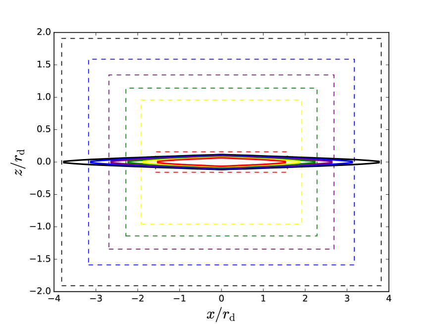
Figure 1: Initial conditions and refinement regions. The black, blue, violet, green, yellow, and red curves show the isodensity contours that contain 90$\%$, 80$\%$, 70$\,\%$, 60$\%$, 50$\%$, and 40$\%$ of the disc mass at $t=0$, respectively. The black, blue, violet, green, yellow, and red dashed lines show the cylinders within which the cell size equals 1/8, 1/16, 1/32, 1/64, 1/128, and 1/256 of the disc exponential scale length, respectively.

Eq. (3) is used to generate random coordinates for a million stellar particles within the optical radius $r_{\rm opt}=3.2r_{\rm d}$ that contains $83\%$ of the mass of the disc (Fujii et al., 2011 demonstrated that numerical heating through close encounters becomes negligible when the disc is resolved with at least a million particles). All stellar particles have equal mass. This article is on stellar discs, but our discs contain a small amount of gas to pave the way for a second article on the formation of bulges in discs with gas. We use a gas fraction of 2$\%$ because in massive low-redshift galaxies the gas fraction varies from close to zero to a few percent and is rarely larger than 5–10$\%$ (for example, Combes et al., 2013), but we also ran four simulations without gas to check the impact that even a small gas fraction could have on our results. The gas in our simulations is isothermal at $10^{4}\,$K and is not allowed to form stars. The total mass of the stellar particles is $0.98\times 0.83\,m_{\rm d}$ in dimensionless virial units.

The circular velocity $v_{\rm c}(r)$ is the speed that a star must have to be on a circular orbit of radius $r$. Its value is the sum in quadrature of the contributions from the disc and the halo:

$$v_{\rm c}^{2}=v_{\rm d}^{2}+v_{\rm h}^{2},$$ (4)

where $v_{\rm d}(r)$ is computed as in Freeman (1970) and

$$v_{\rm h}^{2}={m_{\rm DM}(r)\over r}.$$ (5)

Stars have velocity dispersion:

$$\sigma^{2}(r)=\pi h{m_{\rm d}\over 2\pi r_{\rm d}^{2}}e^{-{r\over r_{\rm d}}}$$ (6)

determined from Eq. (3) through the requirement that our initial condition should be in equilibrium (albeit unstable). Hence, their velocities:

$${\bf v}={\bf v}_{\rm rot}+\Delta{\bf v}$$ (7)

will be the sum of an ordered rotational component (oriented as $\hat{\bf e}_{\phi}$) and a random deviate from a Maxwellian distribution with velocity dispersion $\sigma$. The assumption of an isotropic velocity dispersion is motivated by simplicity, but it is not unreasonable, since the radial and vertical velocity dispersions in the Solar Neighbourhood are $(35\pm 5){\rm\,km\,s}^{-1}$ and $(25\pm 5){\rm\,km\,s}^{-1}$, respectively (Bland-Hawthorn & Gerhard, 2016).

The rotation speed $v_{\rm rot}(r)=\langle v_{\phi}(r)\rangle$ equals the circular velocity $v_{\rm c}(r)$ only for $\sigma=0$. For $\sigma>0$, $v_{\rm rot}$ and $v_{\rm c}$ are linked by the condition:

$$\langle(v_{\rm rot}+\Delta{v}_{\phi})^{2}\rangle=v_{\rm c}^{2},$$ (8)

which gives:

$$v_{\rm rot}^{2}=v_{\rm c}^{2}-\sigma^{2},$$ (9)

since $\langle\Delta v_{\phi}\rangle=0$ and $\langle\Delta v_{\phi}^{2}\rangle=\sigma^{2}$.

Table 1: Simulations with relaxed initial conditions: parameter values and difference in $B/T$ with respect to the unrelaxed simulations.

$\lambda$	$m_{\rm d}$	$c$	$\Delta{B\over T}\,(\%)$
0.025	0.01	5	$-7$
0.025	0.04	5	$-17$
0.050	0.02	5	$+2$
0.025	0.01	15	$-12$
0.025	0.04	15	$+7$
0.050	0.02	15	$-8$

Table 2: Simulations with a live halo: parameter values and difference in $B/T$ with respect to those with a static halo.

$\lambda$	$m_{\rm d}$	$c$	$\Delta{B\over T}\,(\%)$
0.025	0.01	5	$+9$
0.1	0.04	5	$+14$
0.025	0.01	10	$+7$
0.1	0.04	10	$+18$

Table 3: Simulations without gas: parameter values and difference in $B/T$ with respect to those with $f_{\rm gas}=0.02$.

$\lambda$	$m_{\rm d}$	$c$	$\Delta{B\over T}\,(\%)$
0.011	0.01	5	-4
0.011	0.01	10	-9
0.025	0.04	10	-1
0.025	0.04	15	+3

Our rotation speeds and thus our particle velocities are computed using Eq. (9) everywhere except in a small central region where we set $v_{\rm rot}=0$ because $v_{\rm c}<\sigma$. This central region has $r\ll r_{\rm d}$ by construction, since the normalisation of $\sigma(r)$ is determined by the disc scale-height (Eq. 6) and we have assumed that $h\ll r_{\rm d}$. However, the fact that $\sigma$ is computed considering the vertical equilibrium only and that $3\sigma^{2}>v_{\rm c}^{2}$ at $r\lower 2.15277pt\hbox{$\;\buildrel<\over{\sim}\;$}0.07\,r_{\rm d}$ implies that the central region will expand a little bit when the initial conditions are allowed to relax.

The global stability of our initial conditions is explored through the simulations presented in this article (Section 3). Their local stability is a different problem. The discussion of how local disc instabilities can affect the final $B/T$ of globally unstable discs is postponed to Section 4.

2.2 Parameter space

Having fixed the disc scale height $h=0.044\,r_{\rm d}$ and the gas fraction $f_{\rm gas}=0.02$, our initial conditions are entirely determined by three parameters: $r_{\rm d}$, $m_{\rm d}$, and $c$.

	$\lambda=0.011$	$\lambda=0.025$	$\lambda=0.05$	$\lambda=0.1$
$m_{\rm d}=0.005$
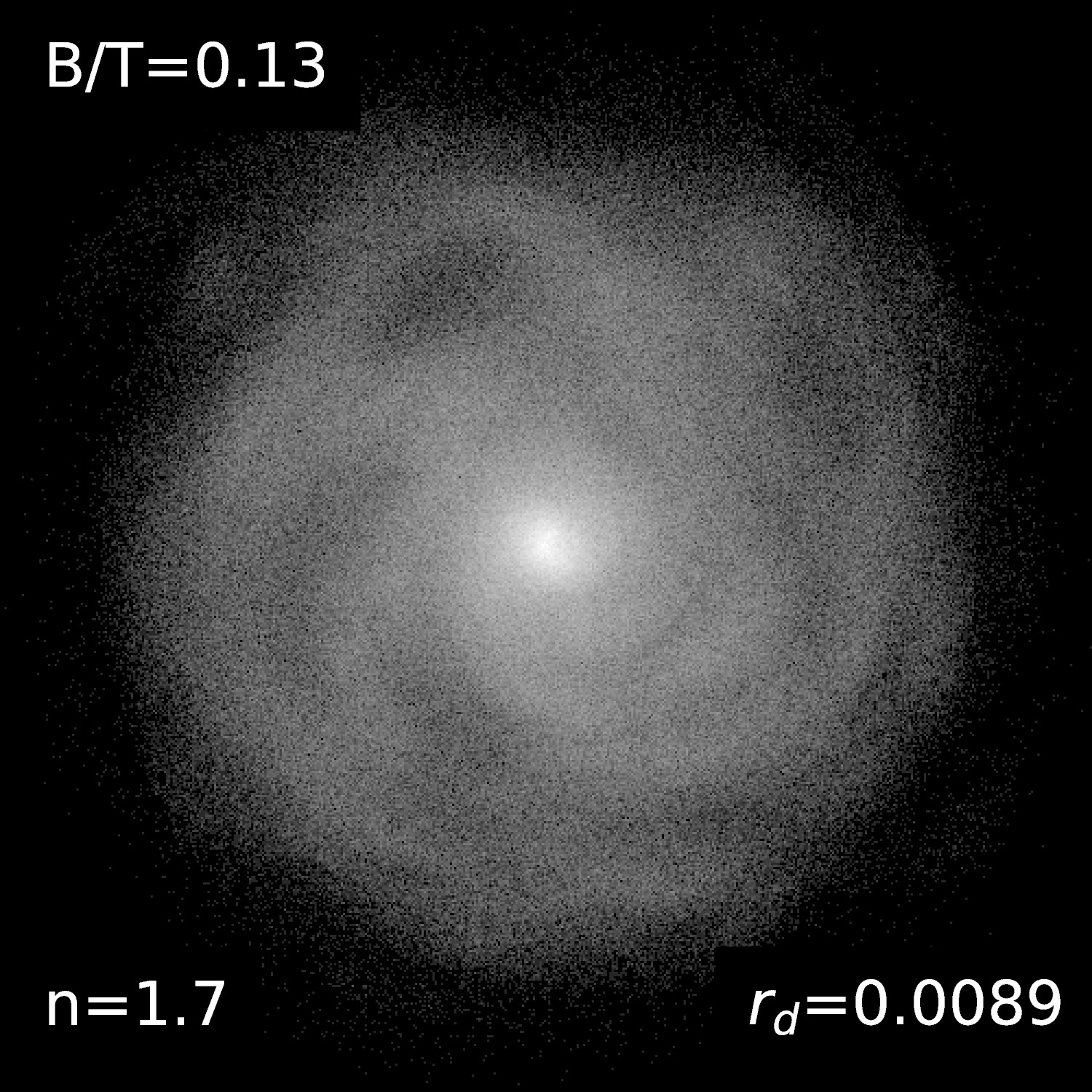
$m_{\rm d}=0.01$
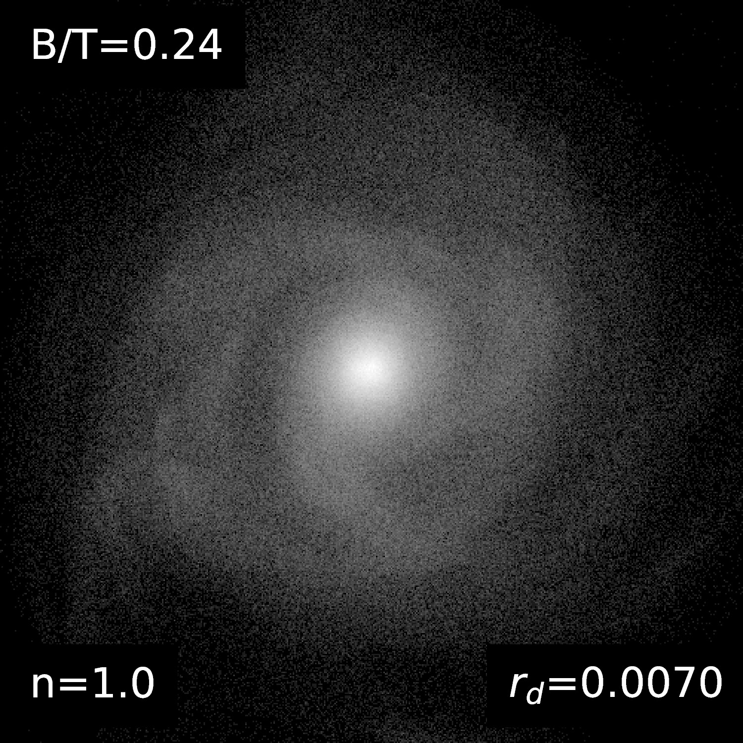
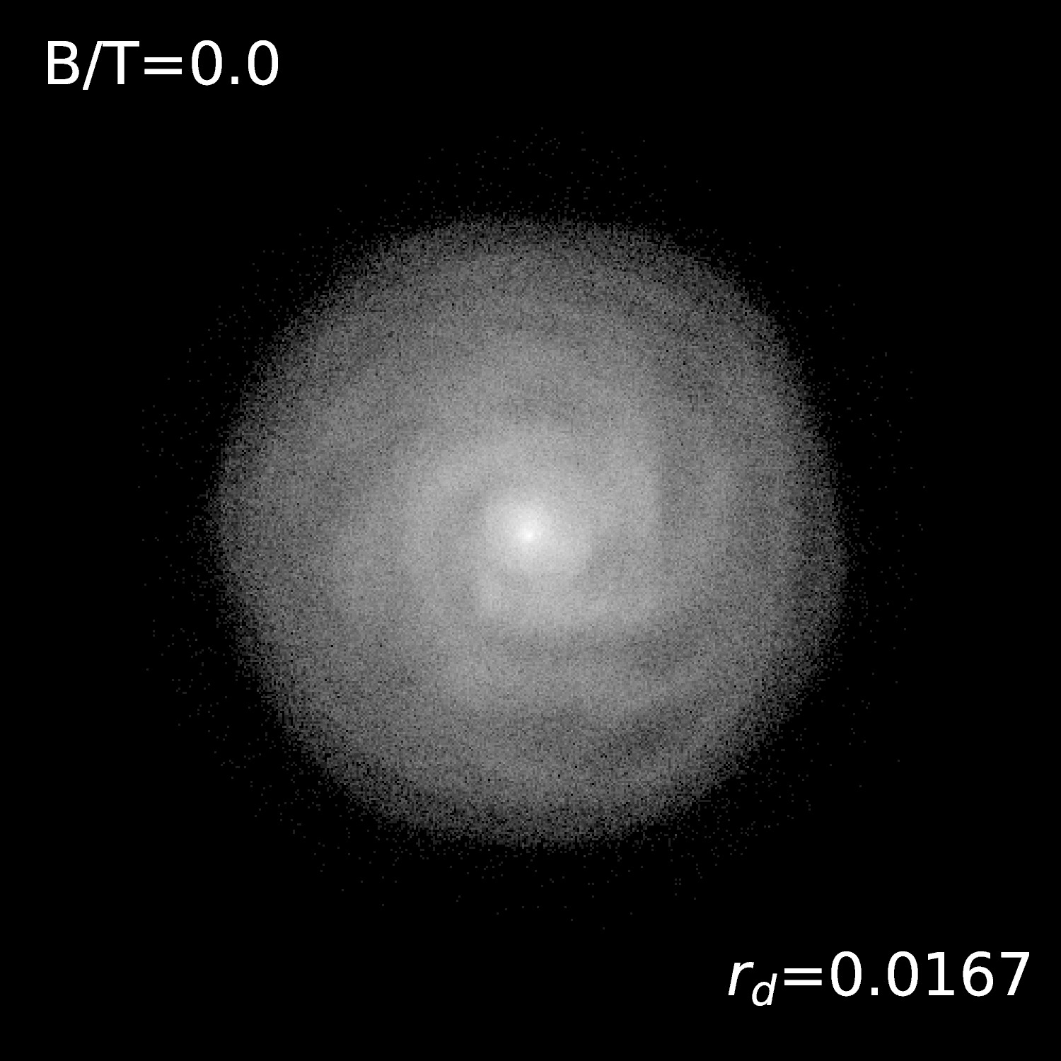
$m_{\rm d}=0.02$
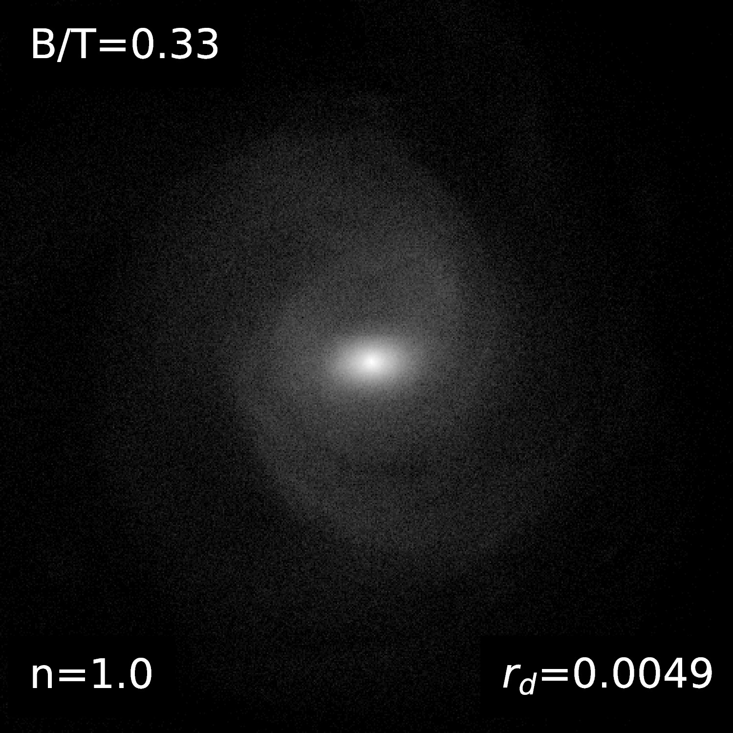
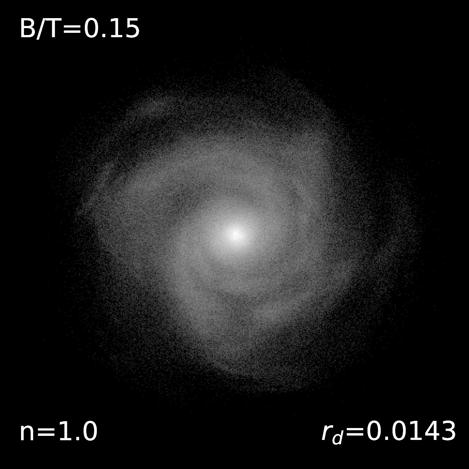
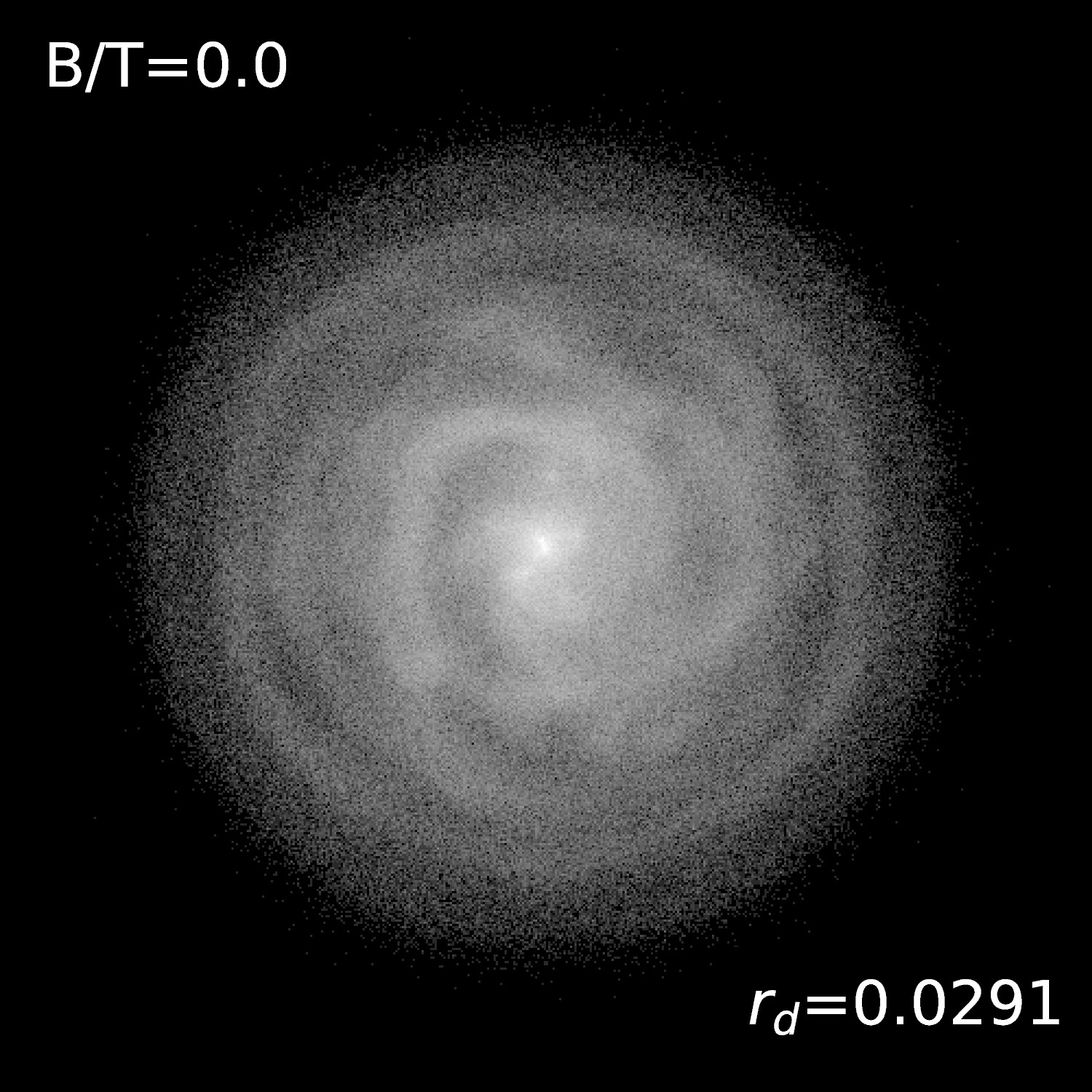
$m_{\rm d}=0.04$

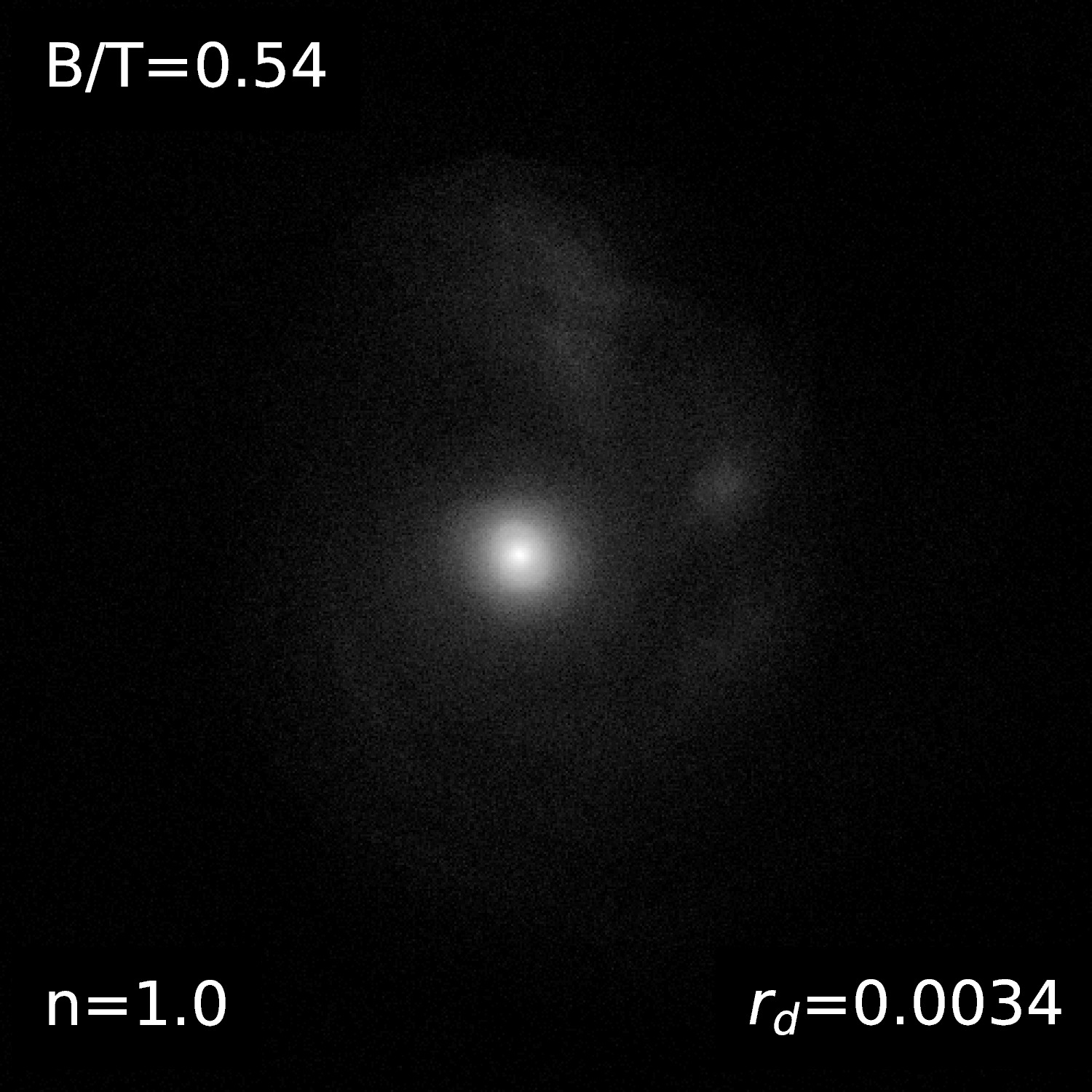
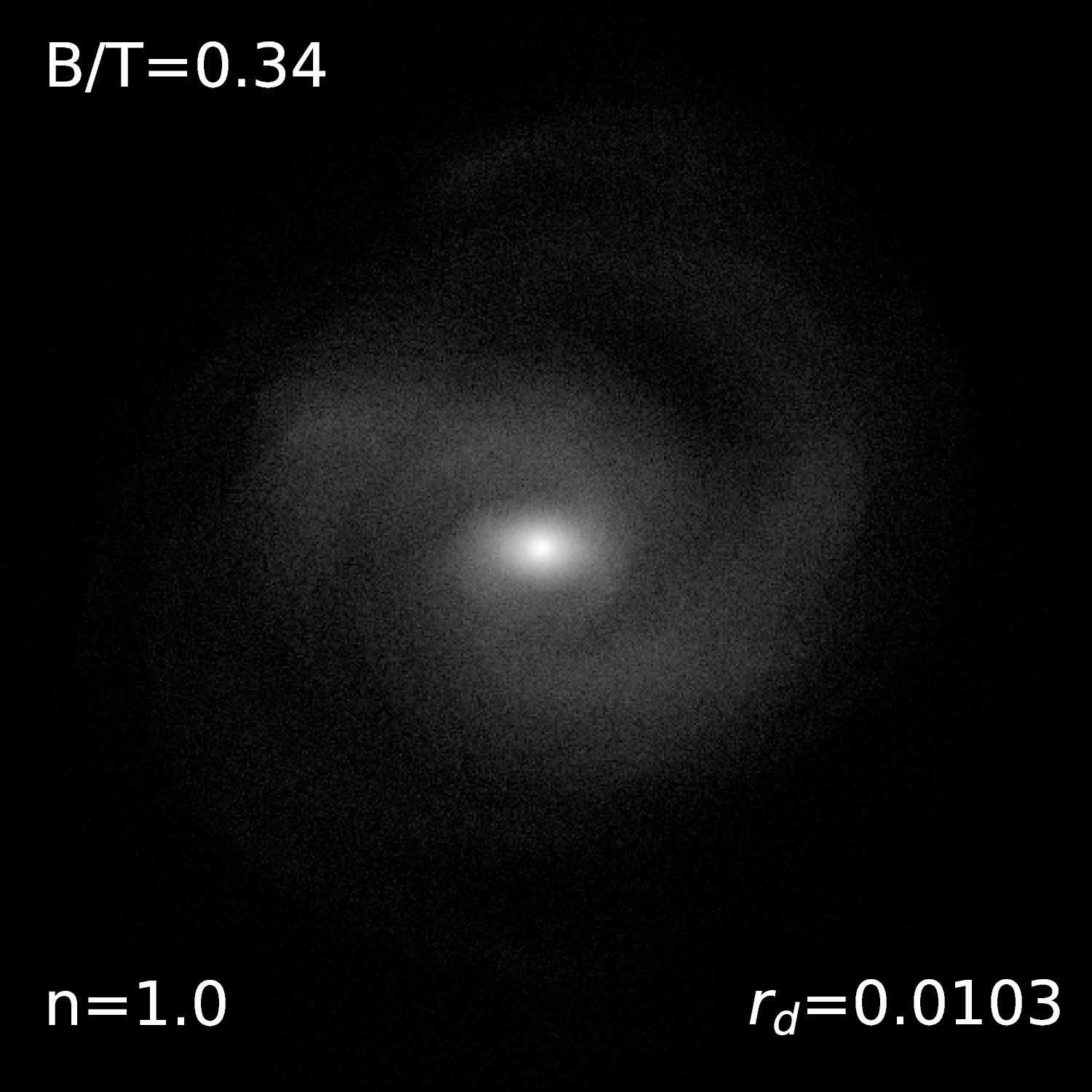
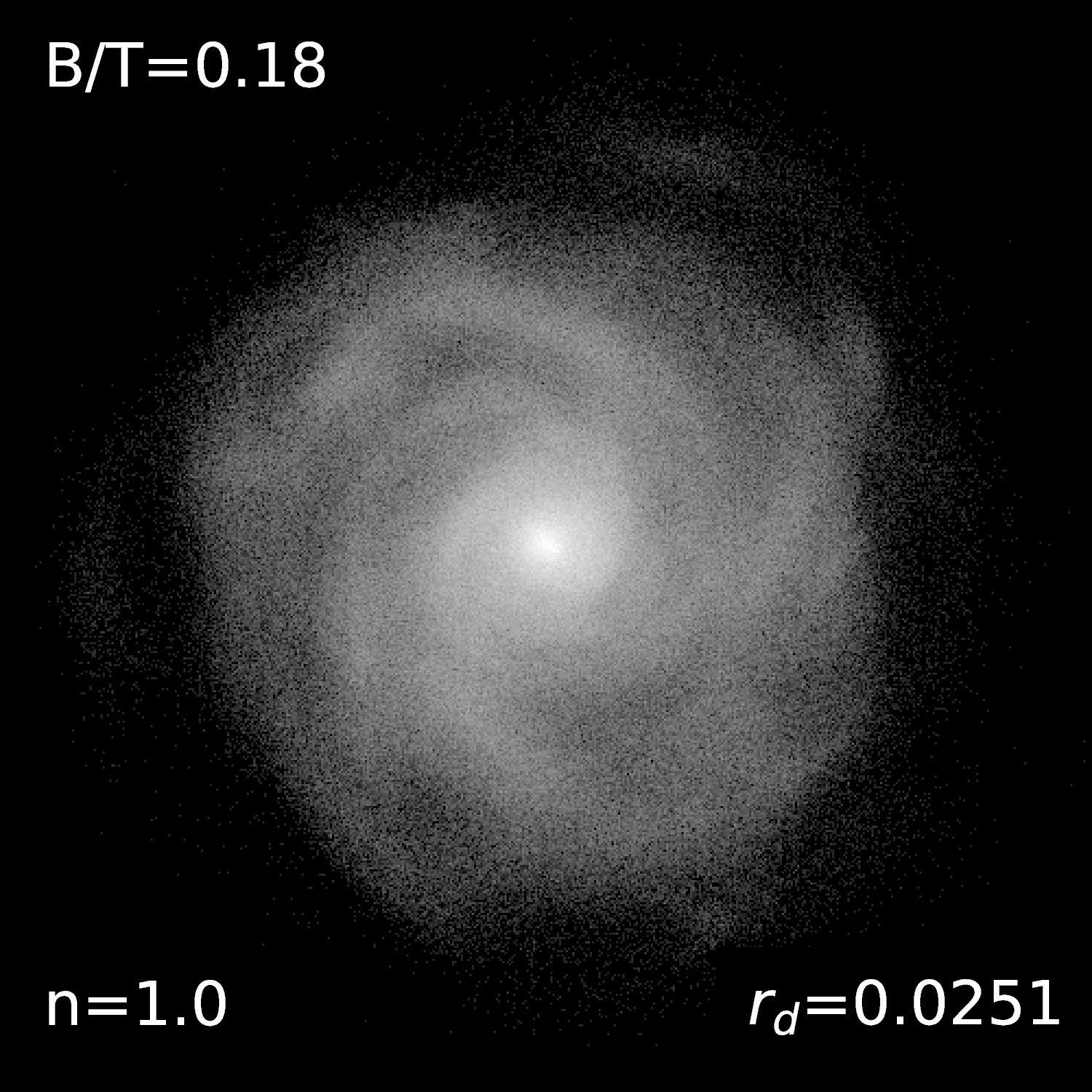
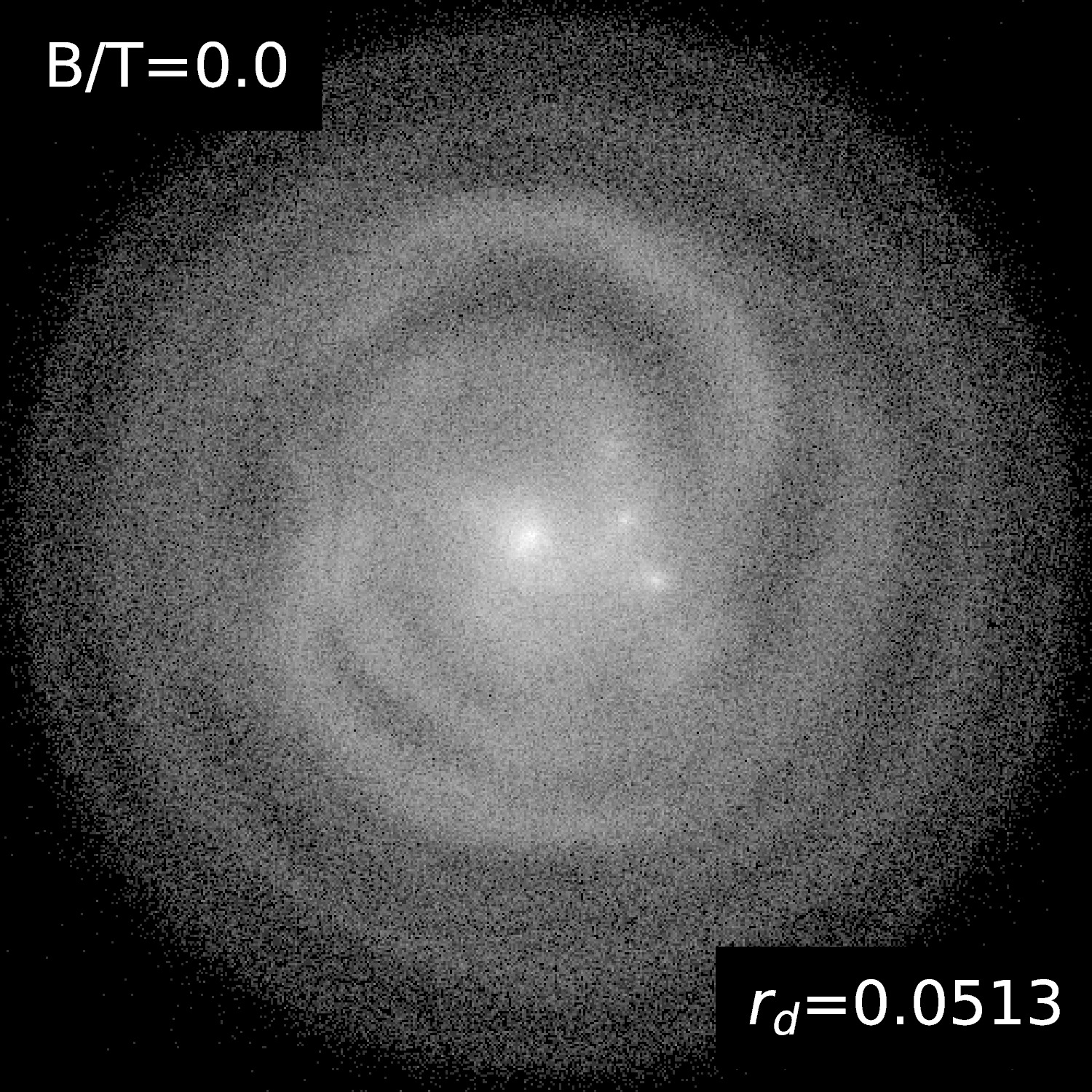
Figure 2: Face-on view of the simulated galaxies at the first time $t$ when $B/T$ has stopped growing ($2{\rm\,Gyr}<t<3{\rm\,Gyr}$). The image brightness is proportional to the logarithm of stellar surface density. This figure show the simulations with $c=5$, sorted by $m_{\rm d}=M_{\rm d}/M_{\rm vir}$ (lines) and halo spin $\lambda$ (columns). On each image, we have shown the corresponding value of $r_{\rm d}=R_{\rm d}/R_{\rm vir}$. Bulge-to-total stellar mass ratios $B/T$ have been computed by decomposing the stellar surface-density distribution into an exponential and a Sérsic (1963) profile. Galaxies that could be fitted with a single exponential profile have $B/T=0$. When the fit required a bulge component, its Sérsic index $n$ has been shown.

	$\lambda=0.011$	$\lambda=0.025$	$\lambda=0.05$	$\lambda=0.1$
$m_{\rm d}=0.005$
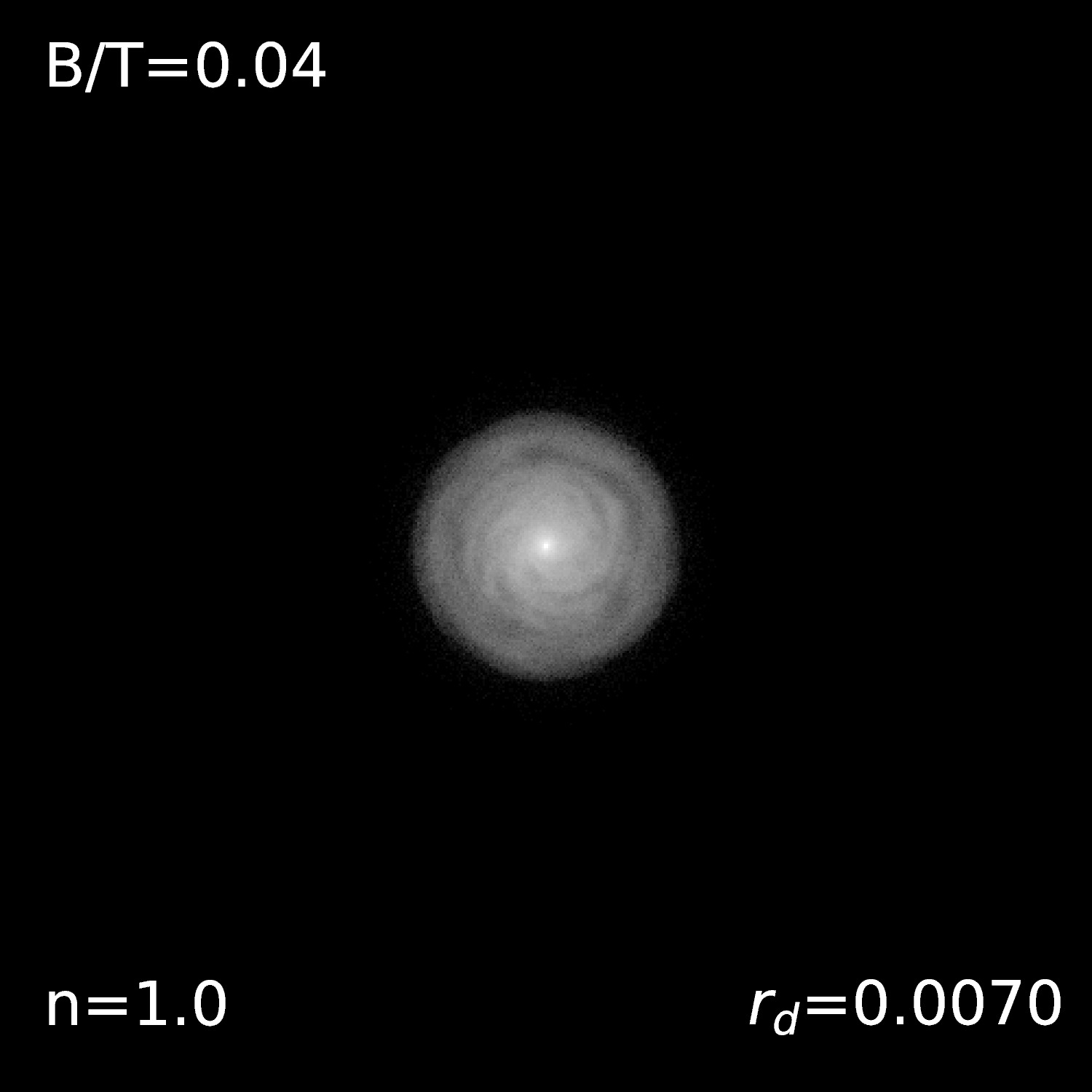
$m_{\rm d}=0.01$
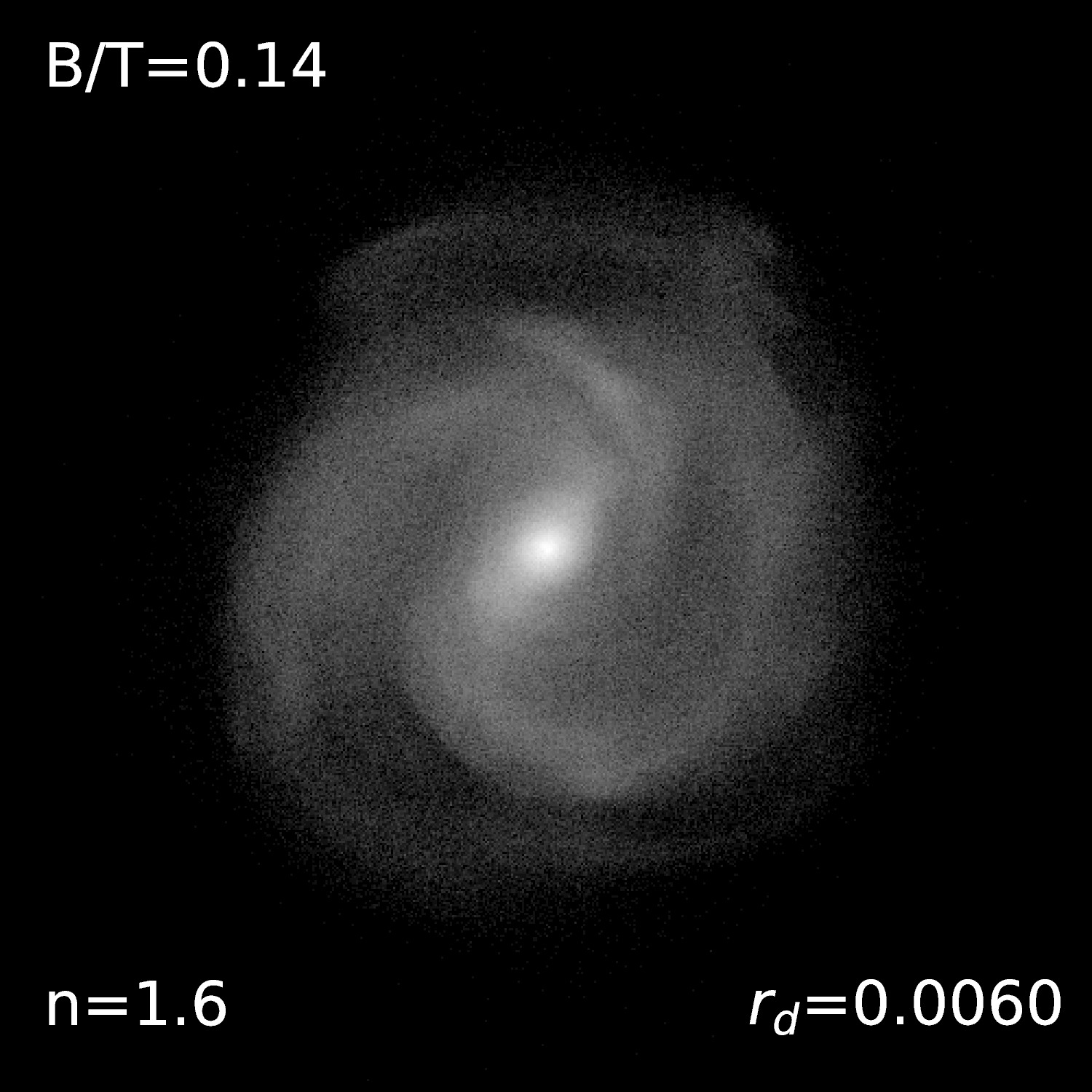
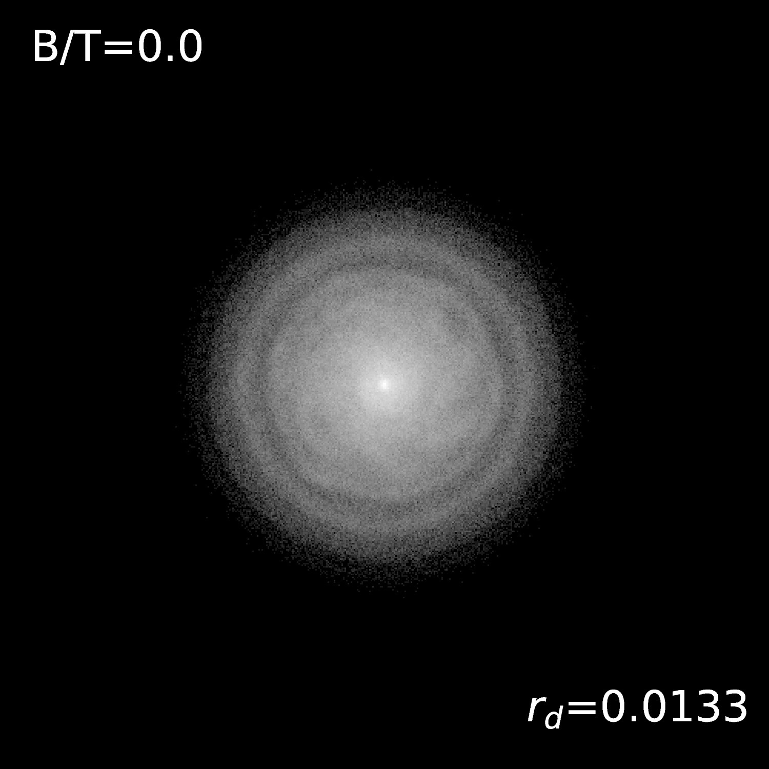
$m_{\rm d}=0.02$
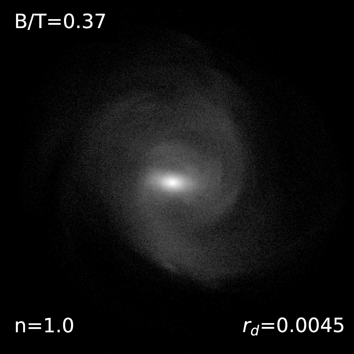
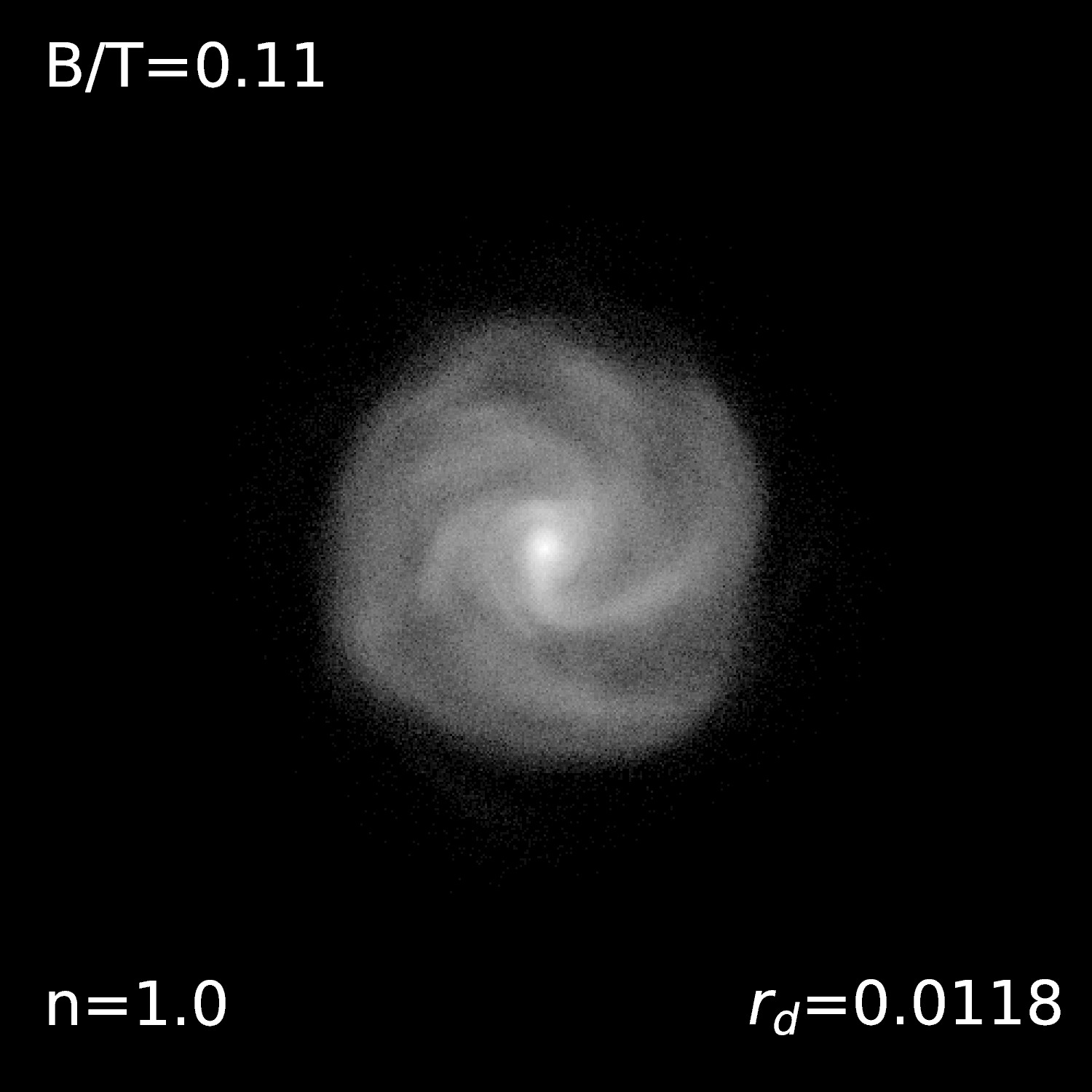
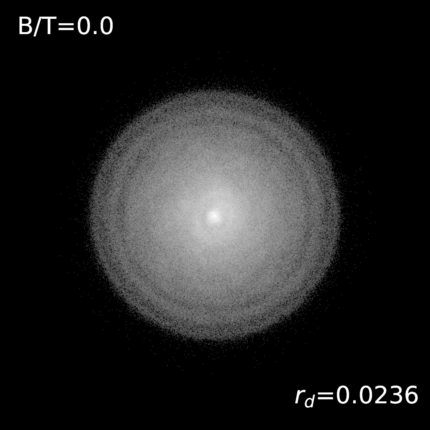
$m_{\rm d}=0.04$

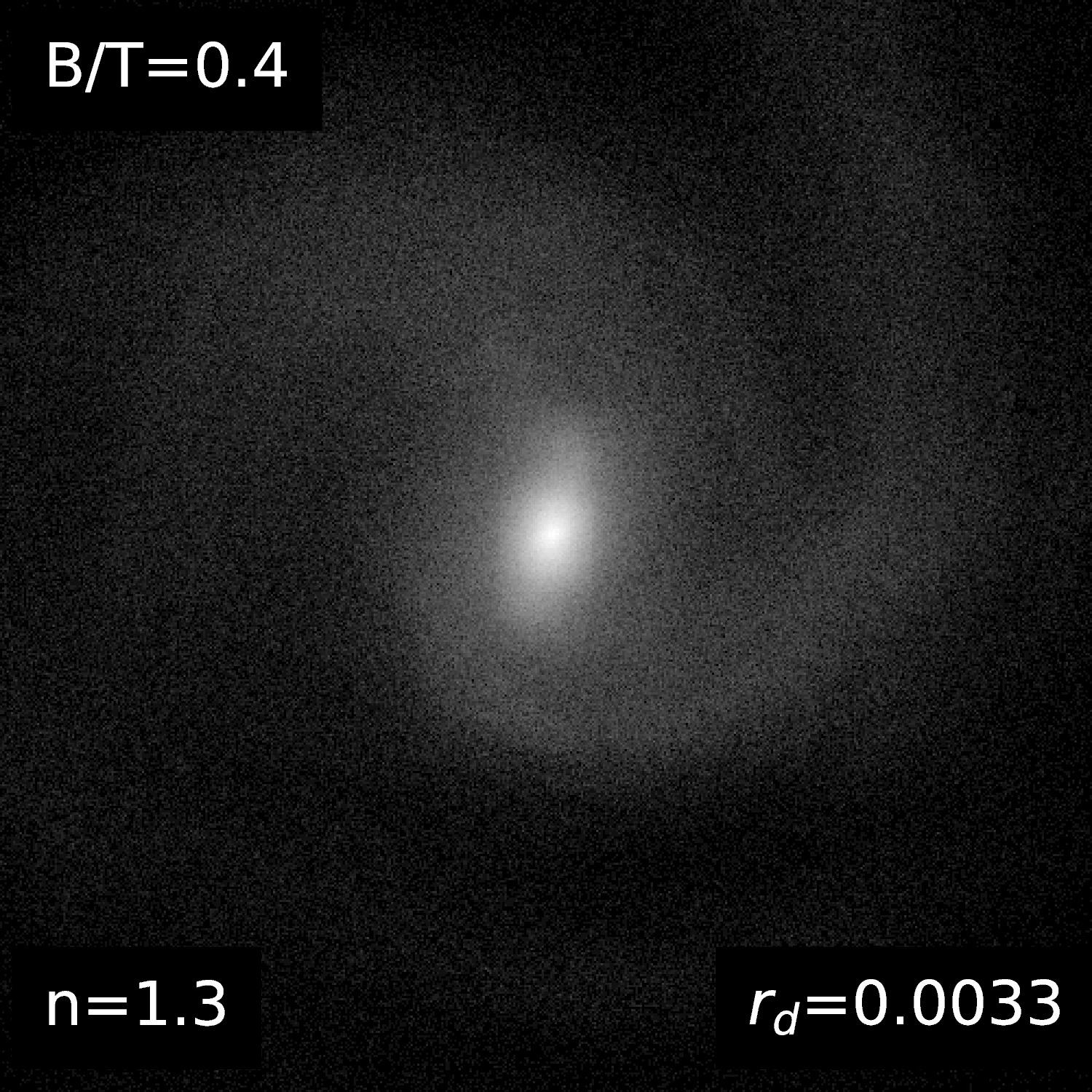
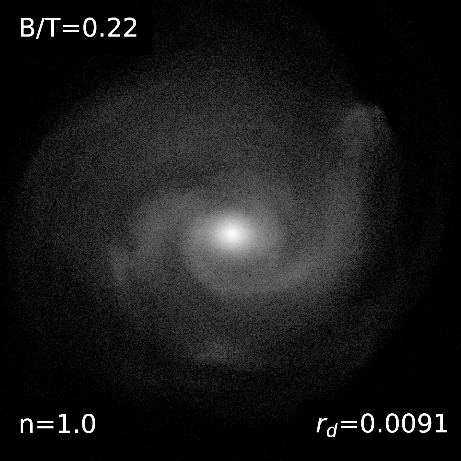
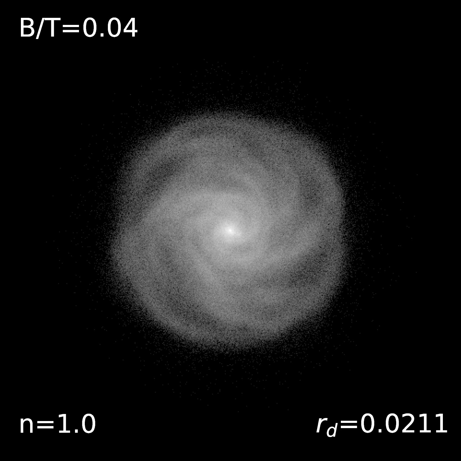
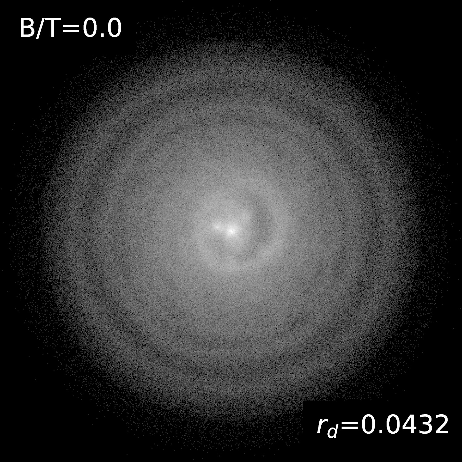
Figure 3: Same as Fig. 2 with $c=10$ instead of $c=5$. To avoid overcrowding the figure, we have not shown the simulations with $\lambda=0.018$ and $\lambda=0.35$.

	$\lambda=0.011$	$\lambda=0.025$	$\lambda=0.05$
$m_{\rm d}=0.005$
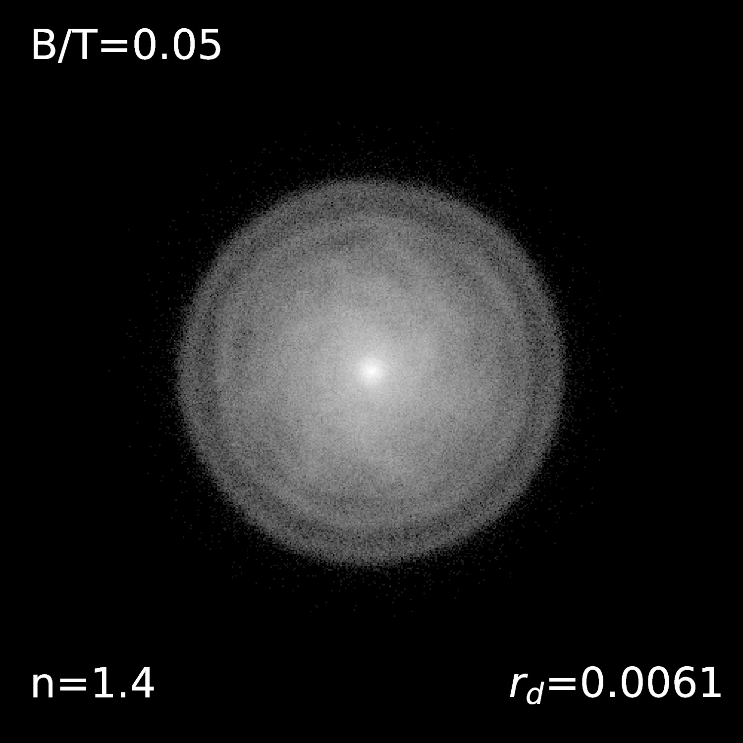
$m_{\rm d}=0.01$
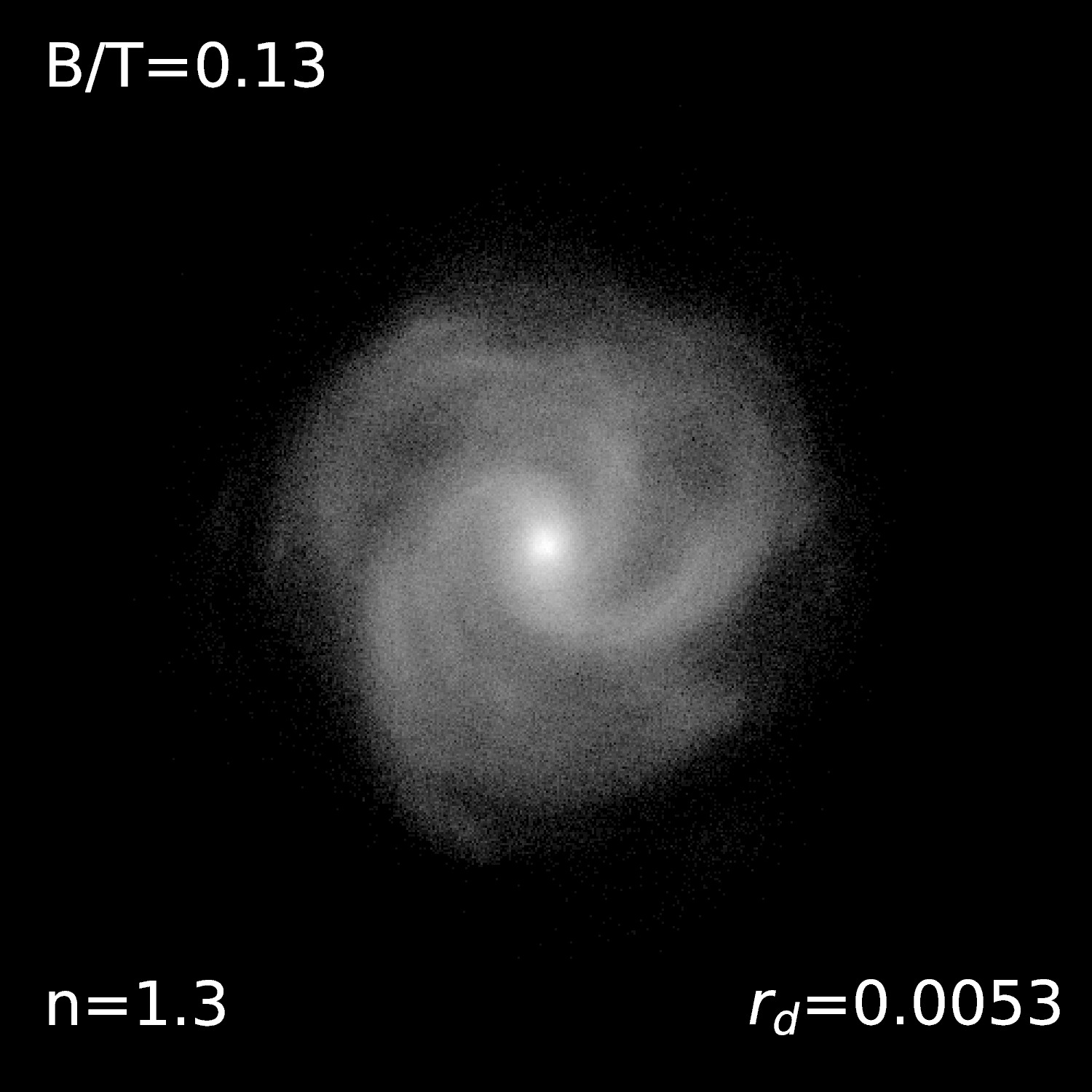
$m_{\rm d}=0.02$
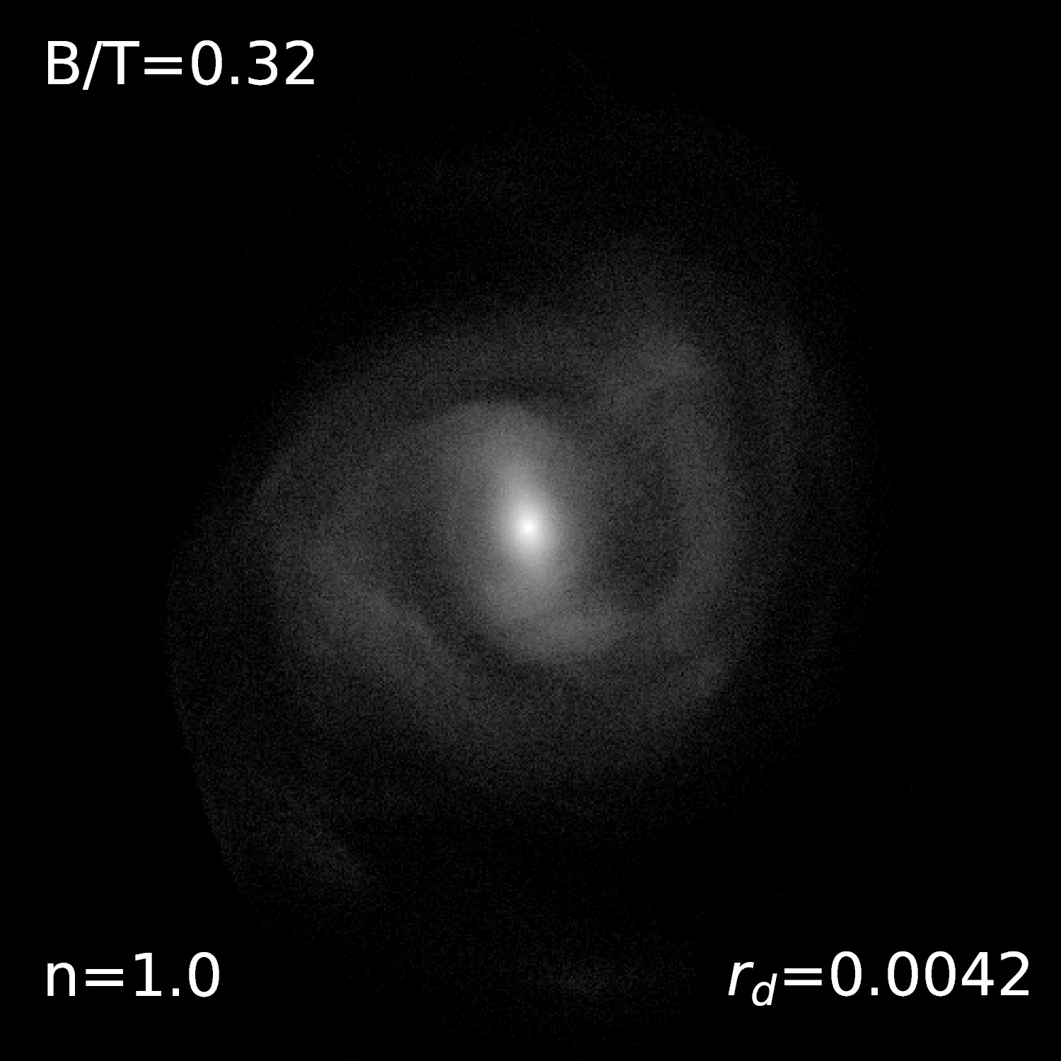
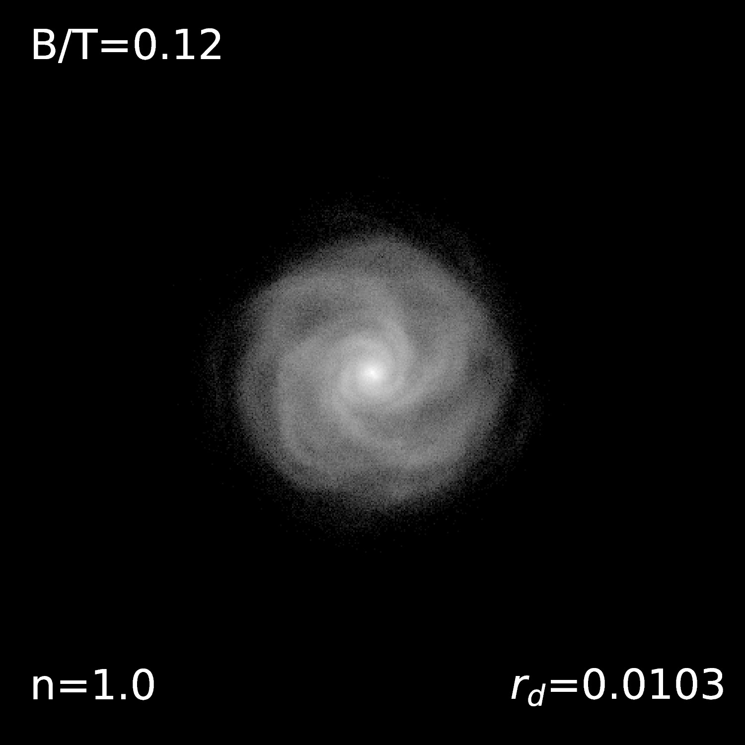
$m_{\rm d}=0.04$

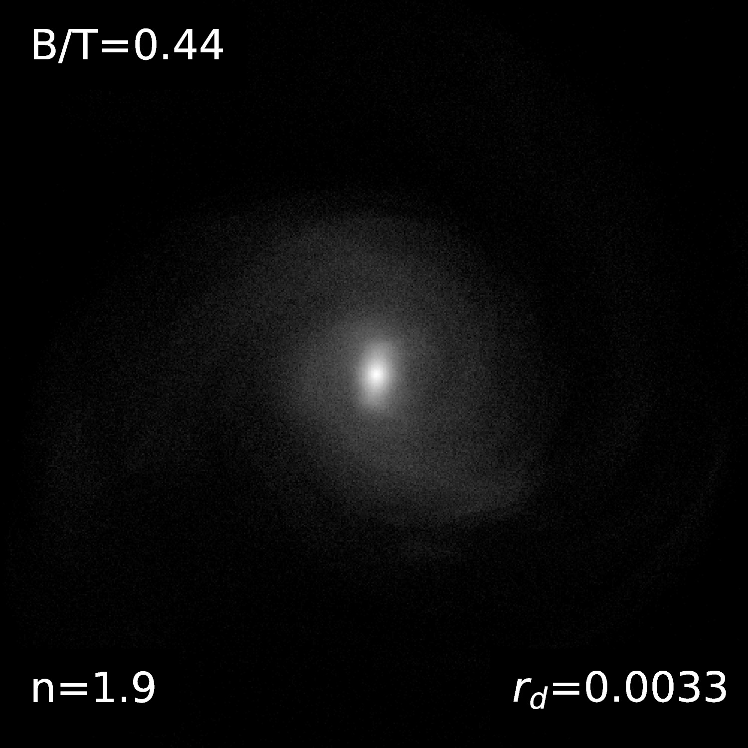
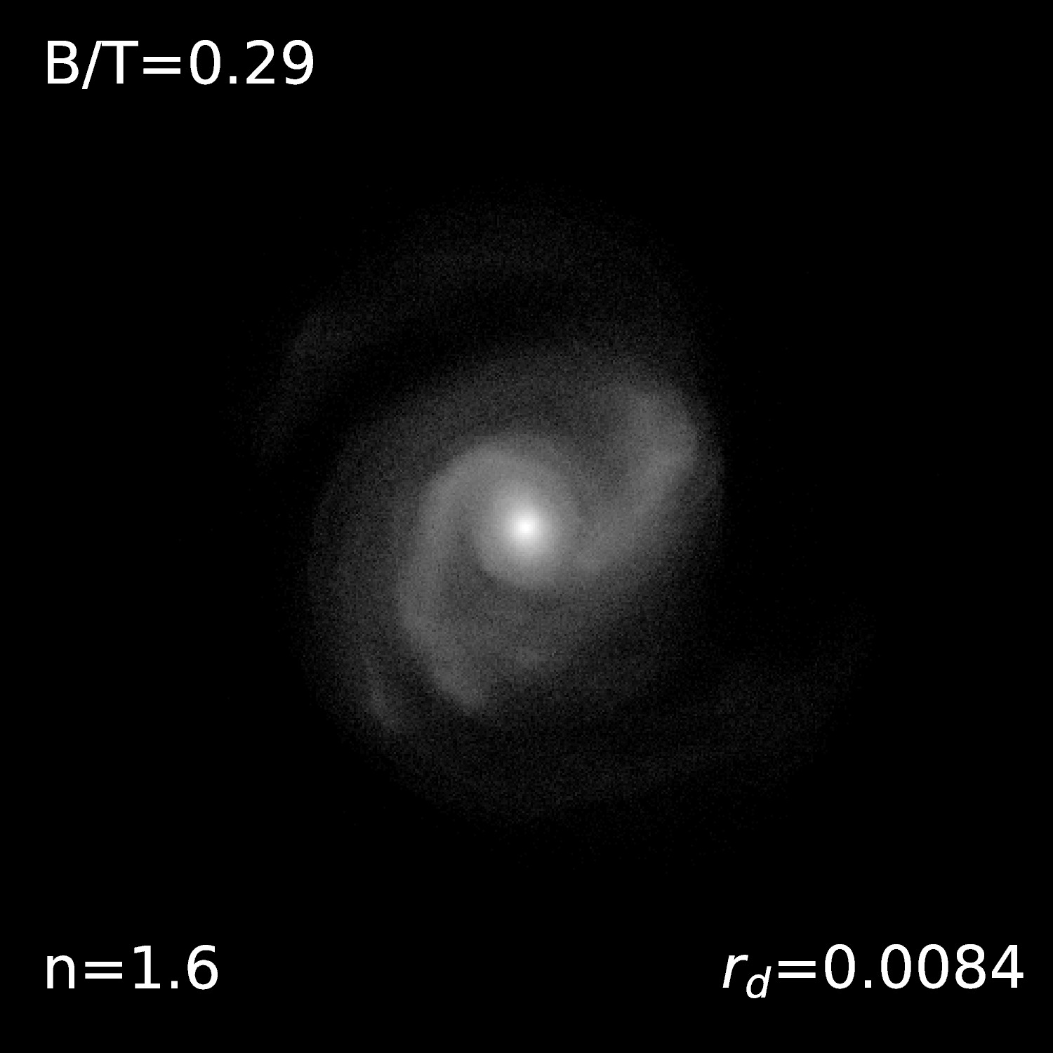
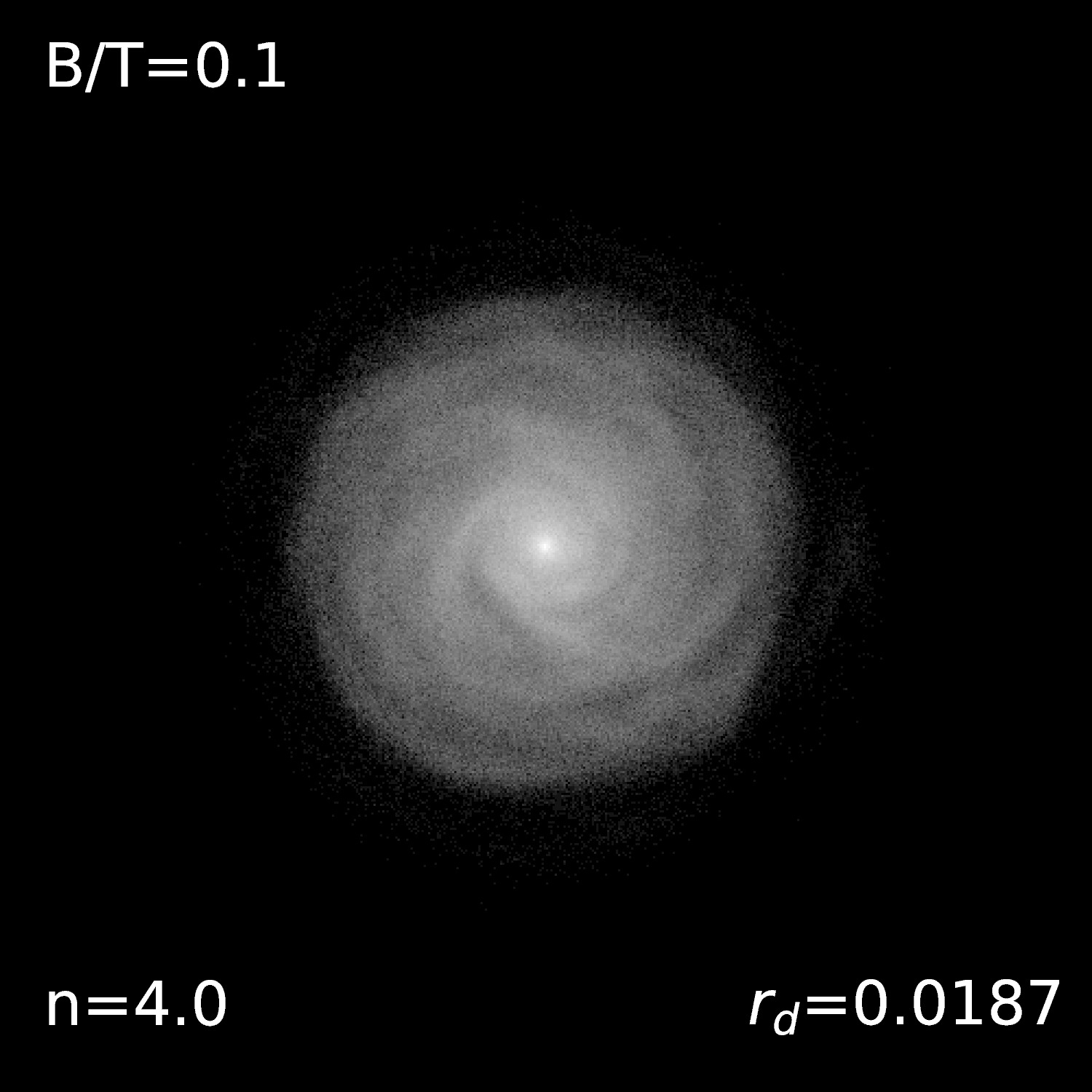
Figure 4: Same as Fig. 2 with $c=15$ instead of $c=5$. The column $\lambda=0.1$ is now missing because we know that simulations with $\lambda=0.1$ will not form any (pseudo)bulge.

The dimensionless radius of a thin exponential disc of dimensionless mass $m_{\rm d}$ embedded in an NFW halo with concentration $c$,

$$r_{\rm d}={\lambda\over\int_{0}^{\infty}e^{-x}v_{\rm c}x^{2}{\rm\,d}x},$$ (10)

(Cattaneo et al., 2017) is completely determined by the disc’s spin parameter

$$\lambda={J_{\rm d}\over M_{\rm d}R_{\rm vir}V_{\rm vir}},$$ (11)

which is identical to the halo’s spin parameter if we follow Mo, Mao, & White (1998) and we assume that the disc and the halo have the same specific angular momentum (for $J_{\rm d}/M_{\rm d}=J_{\rm vir}/M_{\rm vir}$, Eq. 11 corresponds to the Bullock et al., 2001 definition of the spin parameter).

Eq. (10) implies that we can use the spin distribution of DM haloes from cosmological N-body simulations to derive plausible values for $r_{\rm d}$. This is true even if conservation of angular momentum is a crude approximation (Kimm et al., 2011; Stewart et al., 2013; Jiang et al. 2018) because the model by Mo, Mao, & White (1998) reproduces the correct mass – relation for disc galaxies (for example, Cattaneo et al., 2017).

For a flat rotation curve with $v_{\rm c}=1$, Eq. (10) gives $r_{\rm d}=\lambda/2$. We do not make this approximation. We substitute Eq. (4) into Eq. (10) and solve Eq. (10) numerically for each combination of $\lambda$, $m_{\rm d}$, and $c$ that we wish to consider. However, we find that the approximation $r_{\rm d}\simeq\lambda/2$ is accurate at the $20\%$ level.

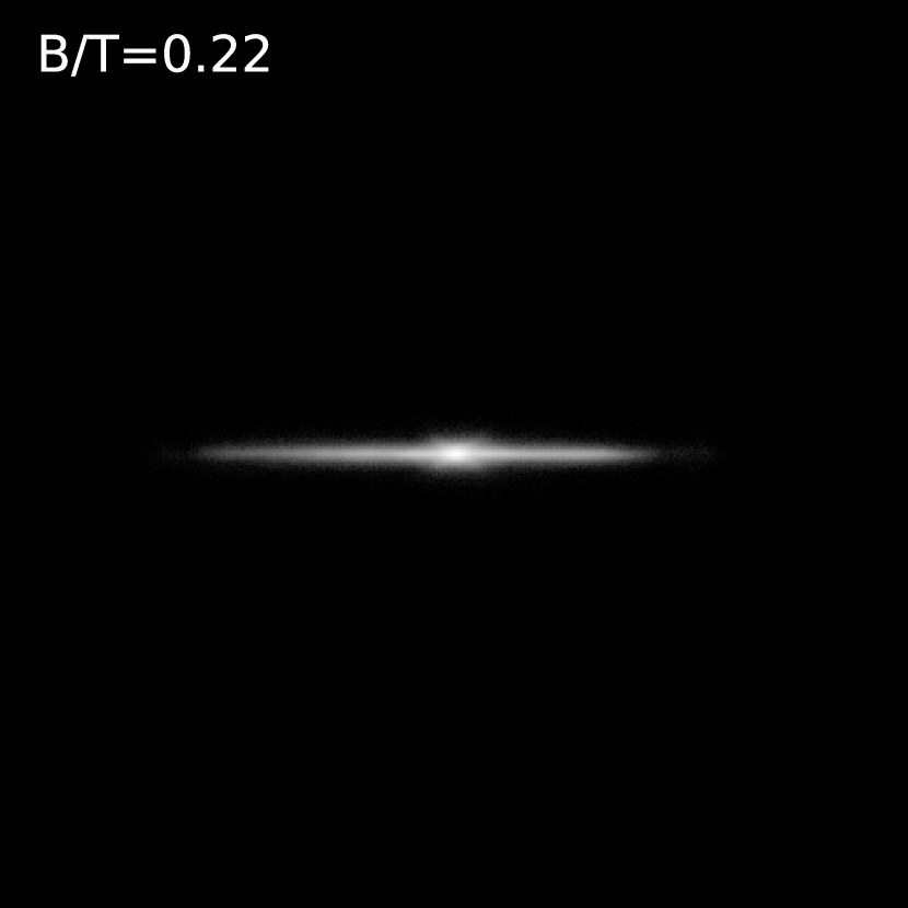
Figure 5: Galaxy in the simulation with $c=10$, $m_{\rm d}=0.04$, $\lambda=0.025$, viewed edge-on. An X-shaped pseudobulge is clearly visible. This galaxy has been chosen as an example and is by no means atypical. The face-on image (Fig. 3) shows that this galaxy has a bar, but not a prominent one.

Muñoz-Cuartas et al. (2011) found that $\lambda$ follows a log-normal distribution with $\bar{\lambda}=0.044$ and $\sigma_{{\rm ln}\,\lambda}=0.57$. Burkert et al. (2016) found a similar distribution with $\bar{\lambda}=0.052$ and $\sigma_{{\rm ln}\,\lambda}=0.46$. So did Cattaneo et al. (2017) with $\bar{\lambda}=0.049$ and $\sigma_{{\rm ln}\,\lambda}=0.57$ (we use the same symbol $\lambda$ for the spin of the halo and the spin of the disc because we have assumed they are identical). From these figures, we conclude that $\lambda=0.05$ corresponds to a typical value and that $\sim 80\%$ of all haloes lie in the interval $0.025<\lambda<0.1$. Haloes with $\lambda<0.0125$ comprise less than $2\%$ of all systems. Based on these considerations and the fact that $r_{\rm d}$ is the parameter to which our results are most sensitive, we have explored six values of $\lambda$ (0.011, 0.018, 0.025, 0.035, 0.05, 0.1).

We sample the parameter space by $\lambda$ rather than $r_{\rm d}$ because we started this research to find a prescription that may be useful to assign morphologies to galaxies in both semianalytic and halo-occupation-distribution models (for example, Behroozi et al., 2013, 2019; Moster et al., 2013, 2018; Tollet et al., 2017). If the objective is to find a recipe to populate haloes with galaxies, then $\lambda$ and $c$ are the quantities that we directly measure in N-body simulations, and we should like to find $B/T$ as a function of them. However, the halo spin has no direct effect on our simulations because our haloes are spherical and static. Hence, it is the dependence of $B/T$ on $r_{\rm d}$ that we probe in reality.

In contrast to $\lambda$, which appears to be a true random quantity, $m_{\rm d}$ strongly correlates with $M_{\rm vir}$. Considerable observational evidence shows that the stellar-to-halo mass ratio increases with $M_{\rm vir}$ over the range of halo masses where spiral morphologies are prevalent (Papastergis et al., 2012; Leauthaud et al., 2012; Reyes et al., 2012; Behroozi et al., 2013; Moster et al., 2013; Wojtak & Mamon, 2013; Cattaneo et al., 2017; Tollet et al., 2017). In a halo with $M_{\rm vir}=10^{12}\,M_{\odot}$, the typical stellar mass of the central galaxy is $M_{\star}=4\times 10^{10}\,M_{\odot}$ ($m_{\rm d}=0.04$ if we assume that the galaxy started as a pure disc). In a halo with $M_{\rm vir}=10^{11}\,M_{\odot}$, the typical stellar mass is two orders of magnitudes lower and $m_{\rm d}$ is lower by about a factor of ten. Hence, we explore four values of $m_{\rm d}$ (0.005, 0.01, 0.02, 0.04) that cover the typical range of $M_{\star}/M_{\rm vir}$ from dwarf to Milky-Way-type galaxies.

$\begin{array}[]{cc}\includegraphics[width=208.13574pt]{bulge.eps}\includegraphics[width=208.13574pt]{nobulge.eps}\end{array}$

Figure 6: Stellar surface-density for two of our simulated galaxies (black symbols). Galaxy $a$ has been fitted with the sum of an exponential profile (blue line) and a Sérsic profile, with $n=1$ in this particular case (red line). Its bulge-to-total mass ratio is $B/T=0.22$. The black curve shows the sum of the two components. Galaxy $b$ is consistent with a single exponential profile (blue line).

Concentration has a much weaker dependence on halo mass. Dutton & Macciò (2014) find $c=10.2M_{12}^{-0.097}$ with $M_{12}=M_{\rm vir}/10^{12}M_{\odot}$ at redshift zero (also see Muñoz-Cuartas et al., 2011). Thus, we expect the mean concentration to vary from $c=13$ for a dwarf galaxy to $c=10$ for a Milky-Way-type one. The real concentration range is larger because the scatter is significant. We thus consider three concentration values (5, 10, 15) such that the interval $5<c<15$ contains $\sim 80\%$ of the haloes with $M_{\rm vir}>10^{11}\,M_{\odot}$.

Six values for $\lambda$, four values for $m_{\rm d}$ and three values for $c$ make $72$ combinations in total. We have simulated only $34$ of these $72$ combinations because we have explored the cases $\lambda=0.018$ and $\lambda=0.035$ only for $c=10$ and because during our work it became obvious that certain sets of parameters would not form a bulge (Section 3). Hence, it would have been pointless to study them.

In addition to these $34$ simulations, we have run another $14$ simulations to address specific issues, such as: 1) relaxation effects due to the assumption of a razor-thin disc, 2) the assumption of a static halo, and 3) the impact of a small gas fraction. The parameter values for these simulations are listed in Tables 1, 2, and 3, respectively. The simulations run for this study are $34+14=48$ in total.

2.3 Refinement strategy

We evolved our initial conditions with the AMR code ramses (Teyssier, 2002) until the galaxies converged to a stable configuration. This usually occurs within $2\,$Gyr.

As we use a Eulerian code, the most important numerical aspect of our work is the choice of the grid on which we integrate the equations of motion for the stellar fluid. We centre our discs on a cubical grid with $128^{3}$ cells and side length $32\,r_{\rm d}$. Hence, the resolution on the scale of the entire computational volume is $l=0.25\,r_{\rm d}$. The resolution is increased within six nested cylinders by a factor of two each time (Fig. 1). The radii $r/r_{\rm d}\simeq 3.8,\,3.2,\,2.7,\,2.3,\,1.9$, and $1.7$ of the six cylinders enclose the isodensity contours that contain 80, 70, 60, 50, 40, and 30$\%$ of the disc mass and correspond to $l/r_{\rm d}=1/8,\,1/16,\,1/32,\,1/64,\,1/128$, and $1/256$, respectively.

Height equals radius in all cylinders except the innermost one, which has a height-to-radius ratio of $1:5$ to ensure than the vertical structure of the thin gaseous disc is well resolved even though the gas fraction in our simulations is so small that it has no dynamical effects. The second innermost cylinder (the one marked in yellow in Fig. 1) has a semi-height ($0.95\,r_{\rm d}$) large enough to ensure that the disc remains well resolved when it buckles up, since the scale-length (and therefore the scale-height) of a pseudobulge is usually several times smaller than $r_{\rm d}$ (Gadotti, 2009).

3 Results

Some of our discs our stable. They do not show any bar or pseudobulge even after $2\,$Gyr. In unstable discs, a bar forms rapidly, but after $2\,$Gyr the growth of $B/T$ becomes very slow and, in many cases, almost inexistent (see below for details of how we measure $B/T$). Figs. 2 to 4 show $27$ simulated galaxies from our main sample of $34$ galaxies in total (we have not shown the simulations $\lambda=0.018$ or $\lambda=0.035$). The galaxies are shown face-on at the first time $t>2\,$Gyr when the growth of $B/T$ has stabilised. In most galaxies, $B/T$ has converged at $t<2.5\,$Gyr.

Figs. 2, 3, 4 correspond to $c=5,\,10,\,15$, respectively. They portray the variety of morphologies that we can reproduce, from Scd to SBa types, simply by changing the values of our parameters. Since our galaxies are isolated and the gas fraction is very small, bar instabilities are the only physical mechanisms through which we expect that a bulge should form in our simulations (see the discussion of this article). In agreement with this expectation, 10 out of 17 galaxies with $B/T>0.1$ display morphologies that are clearly barred. We have also looked at our galaxies edge-on. In most bulges, an X-shaped peanut is clearly visible (Fig. 5).

The galaxy with $m_{\rm d}=0.01$ and $\lambda=0.011$ on Fig. 2 is the most conspicuous example of a prominent bulge ($B/T=0.24$) without any evidence for a bar. Such cases are rare. We have looked at this galaxy edge on. The bulge looks boxy, although the peanut shape is much less obvious than in Fig. 5.

The stellar surface-density profile $\Sigma_{*}(r)$ of each galaxy has been fitted with the sum of an exponential and a Sérsic (1963) profile (Fig. 6a). This decomposition has been used to compute a $B/T$ ratio for each galaxy and a Sérsic index $n$ for the pseudobulges of all galaxies with $B/T>0$. We assume $B/T=0$ when a visual inspection shows the surface-density profile is consistent with a single exponential function (Fig. 6b).

The decrease in $\Sigma_{*}$ in the central region (Fig. 6a) is an artefact due to how we set up the initial conditions for the velocity field. Its cause is the relaxation effect discussed in Section 2.1 after Eq. (9) coupled to the lower resolution in the central region. The radius $r\sim 0.1\,r_{\rm d}$ within which $\Sigma_{*}$ begins to decline is so small that it does not affect our results, except when $B/T$ is very low, in which case it limits our accuracy in fitting the surface-density profile of the bulge component.

All galaxies with $B/T>0.1$ have $n\lower 2.15277pt\hbox{$\;\buildrel<\over{\sim}\;$}1.2$, as expected for pseudobulges. In systems with $B/T\leq 0.1$, the bulge is small and the Sérsic index may not be robust, also because of the effect mentioned above. The galaxy with $m_{\rm d}=0.04$ and $\lambda=0.05$ on Fig. 4 exemplifies this situation. Bulges with $n>2$ are usually classical bulges and are seldom encountered in galaxies with $B/T\lower 2.15277pt\hbox{$\;\buildrel<\over{\sim}\;$}0.1$ (Fisher & Drory, 2008). Hence, our simulations should not form any bulges with $n=4$, let alone one with $B/T=0.1$. A visual inspection of the bulge/disc decomposition shows a poor fit to the stellar surface density in the central region. The Sérsic index $n=4$ measured for this galaxy cannot be considered meaningful.

For given $c$ and $\lambda$, higher values of $m_{\rm d}$ correspond to earlier-type morphologies in the Hubble sequence and to higher $B/T$ (Figs. 2 to 4). We can also increase $B/T$ by reducing $\lambda$ at constant $c$ and $m_{\rm d}$. At constant $\lambda$ and $m_{\rm d}$, $B/T$ usually decreases with $c$. Hence, if a simulation does not form a pseudobulge, simulations with lower $m_{\rm d}$, higher $\lambda$ or higher $c$ will not form one either (supposing the other two parameters were kept fixed). Thanks to this finding, which we have verified in a few cases, we could nearly half the simulations required for this work (there is no need to simulate galaxies for which we know in advance that we shall find $B/T=0$).

The qualitative findings above have a simple interpretation, which will become apparent once we have examined the ELN criterion in greater detail.

For an exponential disc:

$$v_{\rm d}(2.2r_{\rm d})=0.62\sqrt{m_{\rm d}\over r_{\rm d}}=\sqrt{1.3{m_{\rm d}(2.2r_{\rm d})\over 2.2r_{\rm d}}},$$ (12)

where $m_{\rm d}(2.2r_{\rm d})=0.65m_{\rm d}$ is the disc mass within $2.2r_{\rm d}$ (Freeman, 1970). The first equality in Eq.(12) implies that Eq. (1) can be rewritten as:

$${v_{\rm d}(2.2r_{\rm d})\over v_{\rm c}(2.2r_{\rm d})}>{0.62\over\epsilon}.$$ (13)

By introducing the new parameter $\alpha=0.31/\epsilon$, Eq. (13) can be written in the alternative form:

$${v_{\rm d}(2.2r_{\rm d})\over v_{\rm c}(2.2r_{\rm d})}>2\alpha,$$ (14)

where $\alpha=0.28$ for $\epsilon=1.1$ (ELN) and $\alpha=0.26$ for $\epsilon=1.2$ (Christodoulou et al., 1995).

The second equality in Eq. (12) shows that Eq. (14) is equivalent to a criterion on the disc fraction within $2.2r_{\rm d}$ because $v_{\rm c}^{2}(2.2r_{\rm d})/(2.2r_{\rm d})$ is the total gravitational acceleration at $r=2.2r_{\rm d}$ in dimensionless units and $v_{\rm d}^{2}(2.2r_{\rm d})/(2.2r_{\rm d})$ is the disc’s contribution. Therefore,

$$f_{\rm d}(2.2r_{\rm d})=\left[{v_{\rm d}(2.2r_{\rm d})\over v_{\rm c}(2.2r_{\rm d})}\right]^{2}.$$ (15)

is the disc’s fractional contribution to the gravitational acceleration at $r=2.2r_{\rm d}$ and is related to disc’s mass fraction within $2.2r_{\rm d}$ by the equation:

$$f_{\rm d}(2.2r_{\rm d})={1.3m_{\rm d}(2.2r_{\rm d})\over 1.3m_{\rm d}(2.2r_{\rm d})+m_{\rm DM}(2.2r_{\rm d})}.$$ (16)

Van den Bosch (1998) was the first to use the ELN criterion to predict disc stability in a SAM, but he applied Eq. (14) at $r=3r_{\rm d}$ rather than at $r=2.2r_{\rm d}$ for the reason that the rotation curve $v_{\rm c}(r)$ peaks at larger radii when the halo’s contribution is considered. We have verified that Eq. (16) keeps holding at $r=3.2r_{\rm d}$ (the factor $1.3$ does not change to the first decimal digit).

Eqs. (12) and (14) explain why $B/T$ increases with $m_{\rm d}$ and why it decreases with $\lambda$ and $c$ (Figs. 2, 3, and 4). The higher $m_{\rm d}$, the higher the disc fraction within a given radius. The larger the disc, the more DM it will contain. The more concentrated the halo is, the more DM there will be within the disc. Our next step is to go beyond these semi-qualitative considerations and to explore the relation between $B/T$ and $f_{\rm d}$ in quantitative detail.

$\begin{array}[]{cc}\includegraphics[width=208.13574pt]{BT22.eps}\includegraphics[width=208.13574pt]{BT32.eps}\end{array}$

Figure 7: Relation between bulge-to-total mass ratio $B/T$ and initial disc fraction $f_{\rm d}(r)$ for $r=2.2r_{\rm d}$ (left) and $r=3.2r_{\rm d}$ (right). Triangles pointing up, circles, and triangles pointing down correspond to simulations with $c=5$, $c=10$, and $c=15$, respectively. The colours correspond to different disc-to-virial mass ratios: $m_{\rm d}=0.005$ (green), $m_{\rm d}=0.01$ (black), $m_{\rm d}=0.02$ (blue), and $m_{\rm d}=0.04$ (red). Symbols with $B/T=0.01$ correspond to bulgeless galaxies. They have been assigned $B/T=0.01$ merely to be able to show them on a logarithmic diagram. The thick solid black lines are log-log linear least-squares fits to the symbols with $B/T>0.01$. They correspond to Eqs. (18) and (19). The vertical blue lines show the critical $f_{\rm d}$ that corresponds to the $\alpha=0.28$ (equivalent to assuming $\epsilon=1.1$ in Eq. 1) The coloured curves compare our results to previous models (Cole et al., 2000; Hatton et al., 2003; Shen et al., 2003; Cacciato et al., 2012).

Fig. 7 shows $B/T$ versus $f_{\rm d}$ at $r=2.2r_{\rm d}$ (where the rotation curve of an exponential disc peaks) and at the optical radius $r_{\rm opt}=3.2r_{\rm d}$, although we have investigated the relation at other radii down to $r=0.5r_{\rm d}$. The vertical blue lines correspond to:

$$f_{\rm d}^{\rm crit}=(2\alpha)^{2}\simeq 0.31$$ (17)

for $\alpha\simeq 0.28$.

The qualitative picture is the same at $r=2.2r_{\rm d}$ and $r=3.2r_{\rm d}$. At $f_{\rm d}\ll f_{\rm d}^{\rm crit}$, all galaxies are pure discs (the galaxies with $B/T=0.01$ in Fig. 7 are bulgeless galaxies; we have assigned them $B/T=0.01$ merely to be able to show them on a logarithmic plot). At $f_{\rm d}\gg f_{\rm d}^{\rm crit}$, all galaxies develop a pseudobulge and display a tight correlation between $B/T$ and $f_{\rm d}$. At intermediate $f_{\rm d}$, galaxies with $B/T=0$ and $B/T>0$ coexist. Therefore, the ELN criterion may fail to discriminate between stable and unstable discs (Athanassoula, 2008; Fujii et al., 2018). Nevertheless, the notion of a critical $f_{\rm d}$ that separates the two populations remains fundamentally valid.

If we restrict our attention to galaxies with $B/T>0$ and apply a linear least-squares fit to the relation between $\log(B/T)$ and $\log f_{\rm d}$, we find:

$${B\over T}=0.47f_{\rm d}^{2.1}(2.2r_{\rm d})$$ (18)

and

$${B\over T}=0.50f_{\rm d}^{1.8}(3.2r_{\rm d})$$ (19)

(thick black solid lines in Figs. 7a and b, respectively).

Eq. (18) implies $B/T=0.04$ for $f_{\rm d}=f_{\rm d}^{\rm crit}=0.31$. With Eq. (19), $B/T=0.04$ is attained for the slightly lower value $f_{\rm d}=f_{\rm d}^{\rm crit}=0.25$. If we use $B/T=0.04$ as the minimum bulge-to-total stellar mass ratio below which galaxies are effectively bulgeless, then these figures imply that the critical $f_{\rm d}$ is lower at $3.2r_{\rm d}$ than it is at $2.2r_{\rm d}$. This makes sense because $f_{\rm d}(r)$ decreases at large radii in both stable and unstable discs (the density of the baryons in the disc decreases faster than the density of the DM). Hence, it is logical that the critical $f_{\rm d}$ that separates them should decrease with radius, too.

The standard deviation of $\log(B/T)$ from the linear least-squares fit of $B/T$ versus $f_{\rm d}(r)$ (that is, the root-mean-square residuals) decreases slowly but systematically from $0.12\,$dex at $r=0.5r_{\rm d}$ to $0.11\,$dex at $r=3.2r_{\rm d}$. Hence, the ELN criterion is fairly insensitive to the radius at which it is applied, but a criterion at $r=3.2r_{\rm d}$ appears to be preferable.

If the condition $f_{\rm d}^{\rm crit}\simeq 0.31$ is applied at $r=3.2r_{\rm d}$, then all discs with $f_{\rm d}(3.2r_{\rm d})>f_{\rm d}^{\rm crit}$ are correctly identified as unstable (Fig. 7b). For these galaxies, Eq. (19) gives $B/T$ with an accuracy of $\sim 30\%$. In contrast, we find four galaxies with $f_{\rm d}(3.2r_{\rm d})<f_{\rm d}^{\rm crit}$ where the ELN criterion failed to predict instability. However, all these galaxies have $B/T<0.06$. To assume that galaxies with $B/T\lower 2.15277pt\hbox{$\;\buildrel<\over{\sim}\;$}0.06$ are bulgeless is not such a great approximation. Even observers may not be able to detect bulges that small, particularly for galaxies at distances $\lower 2.15277pt\hbox{$\;\buildrel>\over{\sim}\;$}100\,$Mpc.

4 Comparison with previous models

The blue curves and the red curves in Fig. 7 compare our results to the two most common assumptions encontered in SAMs. The blue curves correspond to the model by Cole et al. (2000): as soon as a disc becomes unstable, it collapses into a bulge. The difference from the black lines is plainly obvious. The red solid curves correspond to the model by Hatton et al. (2003) and Shen et al. (2003): as soon as a disc becomes unstable, matter is transferred from the disc to the bulge until the disc is marginally stable.

We compute the analytic form of the red curves by assuming that initially all the stars are in the disc, so that the stellar masses within $2.2\,r_{\rm d}$ and $3.2\,r_{\rm d}$ are $0.65\,m_{*}$ and $0.83\,m_{*}$, respectively. Eq. (16) gives:

$${\beta m_{*}\over\beta m_{*}+m_{\rm DM}}=f_{\rm d},$$ (20)

with $\beta=1.3\times 0.65=0.85$ or $\beta=1.3\times 0.83=1.1$, depending on the radius at which the instability condition is considered ($m_{\rm DM}$ is the mass of the DM within this radius). The disc becomes marginally stable when:

$${\beta(m_{*}-m_{\rm b})\over\beta(m_{*}-m_{\rm b)})+m_{\rm b}+m_{\rm DM}}=f_{\rm d}^{\rm crit},$$ (21)

where $m_{\rm b}$ and $m_{*}-m_{\rm b}$ are the final bulge mass and the final disc mass, respectively. We compute the final bulge fraction $B/T=m_{\rm b}/m_{*}$ by solving Eqs. (20) and (21), and find:

$${B\over T}={1\over 1+(\beta^{-1}-1)f_{\rm d}^{\rm crit}}\left(1-{f_{\rm d}^{\rm crit}\over f_{\rm d}}\right),$$ (22)

where $f_{\rm d}^{\rm crit}\leq f_{\rm d}\leq 1$. Eq. (22) shows that $B/T\rightarrow 0$ for $f_{\rm d}\rightarrow f_{\rm d}^{\rm crit}$ and that:

$${B\over T}\rightarrow{1-f_{\rm d}^{\rm crit}\over 1+(\beta^{-1}-1)f_{\rm d}^{\rm crit}}$$ (23)

for $f_{\rm d}\rightarrow 1$. The limit for $f_{\rm d}\rightarrow 1$ reduces to $B/T\rightarrow 0.71$ for $f_{\rm d}^{\rm crit}=0.31$ and $\beta=1.1$.

The red solid curves are in better agreement with the symbols than the blue curves, but they systematically overestmate $B/T$ at high masses and underestimate it at low masses. The red dashed curves show that increasing $f_{\rm d}^{\rm crit}$ does not improve the overall agreement between Eq. (22) and the simulations because it reduces the discrepancy with the symbols at high $f_{\rm d}$, but it makes it worse at low $f_{\rm d}$.

We have also compared our results to a third model based on the conservation of energy (Cacciato et al., 2012). The specific energy of the stars in a cold disc is:

$$e={1\over 2}v_{\rm c}^{2}+\Phi,$$ (24)

where $\Phi$ is the gravitational potential. When stars migrate from the disc to the bulge, they move to a lower energy level. The gravitational energy released by this process increases the stellar velocity dispersion $\sigma$. Cacciato et al. (2012) used the conservation of energy to study the evolution of two-component discs (gas plus stars) in a cosmological context. Here, we consider a simpler version of their model, in which the disc is isolated (there is no accretion) and purely stellar (there is no gas and thus no star formation). The internal energy of the stars, ${3\over 2}M_{*}\sigma^{2}$, equals the energy released by the formation of a bulge, $M_{\rm b}\Delta e$.

To compute $\Delta e$, one should know the initial and final radii of the stars that migrated to bulge, but one can expect $\Delta e\sim V_{\rm c}^{2}$ within a factor of order unity (Cacciato et al., 2012) and compute $B/T=M_{\rm b}/M_{*}$ by solving the equation:

$$M_{\rm b}V_{\rm c}^{2}\simeq{3\over 2}M_{*}\sigma^{2}.$$ (25)

The calculation of $\sigma$ is based on the assumption that $\sigma$ self-regulates so that the Toomre (1964) stability parameter is always close to critical value $Q_{\rm c}$ for local stability. This assumption gives:

$${\sigma\Omega\over{\rm G}\Sigma}=Q_{\rm c},$$ (26)

with $Q_{\rm c}=1.68$ for a razor-thin sheet of stars with a Maxwellian velocity distribution (see Binney & Tremaine, 2008).

Let expand Eq. (26) by using $\Omega=V_{\rm c}/R$:

$$\sigma={{\rm G}\Sigma R\over V_{\rm c}}Q_{\rm c}={{{\rm G}\Sigma R^{2}\over R^{2}}\over{V_{\rm c}^{2}\over R}}Q_{\rm c}V_{\rm c}.$$ (27)

$V_{\rm c}^{2}(R)/R$ is the total gravitational acceleration at radius $R$. The numerator measures the disc’s contribution after the formation of a bulge (the mass of the disc within $R$ scales as $\Sigma R^{2}$). This contribution can be decomposed into the product of two terms: the stellar contribution relative to the total stars plus DM (the $f_{\rm d}$ factor, since all the stars are in the disc at $t=0$) and the stellar fraction in the disc after a bulge has formed, $M_{\rm d}/M_{*}$. The product is not exact because matter changes geometry when it migrates from the disc to the bulge, but neglecting that has a small effect. Eq. (27) can thus be rewritten:

$$\sigma\simeq\eta f_{\rm d}(R){M_{\rm d}\over M_{*}}Q_{\rm c}V_{\rm c},$$ (28)

where $\eta$ is a fudge factor (the disc mass within $R$ scales as, but is not equal to, $\Sigma R^{2}$).

By substituting Eq. (28) into Eq. (25) and using $M_{\rm d}=M_{*}-M_{\rm b}$, we find:

$${M_{\rm b}\over M_{*}}\simeq{3\over 2}\eta^{2}Q_{\rm c}^{2}f_{\rm d}^{2}\left(1-{M_{\rm b}\over M_{*}}\right)^{2},$$ (29)

where all uncertainties, and notably the one on $\Delta e/V_{\rm c}^{2}$, are reabsorbed in the value of $\eta$.

It is straightforward to solve the second-degree Eq. (29) and compute $B/T$ as a function of $f_{\rm d}$. The results are shown by the green curves on Fig. 7. The best agreement with our simulations is for $\eta=0.41$.

The model by Cacciato et al. (2012) predicts a shallower slope for $B/T$ versus $f_{\rm d}$ than what we find in our simulations, especially at high $f_{\rm d}$ and when it is applied at $r=2.2\,r_{\rm d}$. However, it is the model that works best.

5 Comparison with observations

Our simulations predict that $B/T$ is related to $V_{\rm d}/V_{\rm c}$. Persic & Salucci (1995) and Persic et al. (1996) used 967 galaxies with $I$-band photometry and H$\alpha$ data from Mathewson et al. (1992) to conduct one of the most careful and systematic study of the rotation curves of galaxies. The main result from Persic et al. (1996) was that $V_{\rm d}/V_{\rm c}$ increases with $I$-band luminosity from $V_{\rm d}(R_{\rm opt})/V_{\rm c}(R_{\rm opt})=0.4$ at $M_{I}=-18.5$ to $V_{\rm d}(R_{\rm opt})/V_{\rm c}(R_{\rm opt})=0.96$ at $M_{I}=-23.2$, where $R_{\rm opt}=3.2R_{\rm d}$ (the brightest discs are close to being maximal). This finding is just another way to say that the stellar-to-total mass ratio increases with stellar mass (for example, Dekel & Silk, 1986; Papastergis et al., 2012; Behroozi et al., 2013; Moster et al., 2013). We can use it to transform Eq. (19) into a prediction for how $B/T$ grows with $I$-band luminosity (Fig. 8, black curve). In this section, we use three data sets to compare this prediction with observations.

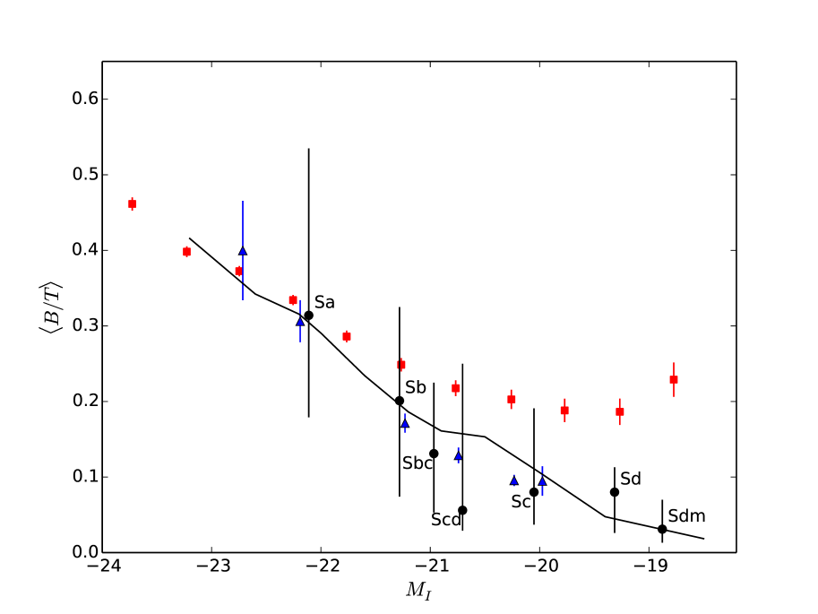
Figure 8: $\langle B/T\rangle$ versus $I$-band magnitude $M_{I}$. The black curve shows our prediction. The black circles are from Mathewson et al. (1992) when we assign to each Hubble type the $\langle B/T\rangle$ from Graham & Worley (2008; the uncertainty of estimating $B/T$ determines the size of the error bars). The red squares are from Simard et al. (2011) after removing all galaxies with $B/T>0.7$. The up-pointing filled blue triangles and the down-pointing empty blue triangles are from Salo et al. (2015, S⁴G) when we assign the bar to the bulge and the disc, respectively. The error bars on the red squares and the blue filled triangles show the standard error on the mean. We have not shown the error bars on the empty triangles so that they do not overlap with those on the filled triangles, but their width is comparable.

The catalogue in Mathewson et al. (1992) contains only 1355 galaxies and no quantitative morphologies, but it has the advantage of being the parent sample in Persic & Salucci (1995): using the morphology – luminosity relation from the same data set that we have used to pass from $V_{\rm d}(R_{\rm opt})/V_{\rm c}(R_{\rm opt})$ to $M_{I}$ ensures that our analysis is internally consistent.

Hubble-type information can obviate the lack of quantitative morphologies. In Fig. 8, the black circles with error bars show the mean $B/T$ from Graham & Worley (2008) and the mean $I$-band magnitude $M_{I}$ in the catalogue from Mathewson et al. (1992) for each Hubble type. Our predictions are in good agreement with the black circles within the observational uncertainties. The analysis by Hubble type has two limitations, however. First, Hubble type is not a quantitative measurement of $B/T$. Second, we have not considered the frequency of different Hubble types in Mathewson et al. (1992)’s catalogue (Table 4).

Simard et al. (2011) fitted the $r$-band surface-brightness profiles of $1.12$ million galaxies from the SDSS with a Sérsic plus exponential model. Their $B/T$ values are therefore directly comparable to ours (to the extent that $r$-band luminosity traces stellar mass).

To pass from $r$ to $I$-band, we use Lupton’s formula:

$$M_{I}=M_{i}-0.3780(M_{i}-M_{z})-0.3974.$$ (30)

We retrieve $M_{i}$ and $M_{z}$ for galaxies in the SDSS Data Release 7 (DR7) by using the selection query:

SELECT
  objid, ra, dec, run, camcol, rerun,
  petromag_i, petromag_z,
  extinction_i, extinction_z
FROM
  PhotoPrimary
WHERE
  flags
  AND (dbo.fPhotoFlags(’SATURATED’)+
  dbo.fPhotoFlags(’DEBLENDED_AS_PSF’))= 0
  AND (petroMag_r- extinction_r)
  BETWEEN 14.0 and 18.0
  AND Type=3

and by cross-correlating the results with the catalogue from Simard et al. (2011).

Table 4: Morphological composition of the catalogue in Mathewson et al. (1992). Hubble types $T$ are from de Vaucouleurs et al. (1976).

Class	$T$	$N_{\rm gal}$
Sa	1	1
Sab	2	0
Sb	3	362
Sbc	4	124
Sc	5	114
Scd	6	558
Sd	7	34
Sdm	8	66
Sm	9	0
Im	10	1

This sample selection includes elliptical galaxies, while we are interested in the $B/T$ – $M_{I}$ relation for spiral galaxies. We circumvent this problem by removing all bona fide ellipticals with $B/T>0.8$ and $n>2$. This selection is based on the distribution of galaxies on a $B/T$ versus $n$ diagram (Fig. 14 of Simard et al., 2011), which shows two main populations: a spiral/S0 population with $0<B/T<0.7$ and $0<n<7$ (the mean $B/T$ grows with $n$), and an elliptical population with $B/T>0.8$ and $n>2$. The diagram also shows a third population with $B/T>0.7$ and $n<1.5$ (most of these galaxies have $B/T\sim 1$). Visual inspection (for example, Fig. 9) suggests that the bulges of these galaxies are misclassified discs (discs for which a Sérsic model with $n<1$ worked better than an exponential fit). We therefore assign $B/T=0$ to galaxies for which Simard et al. (2011) find $B/T>0.7$ and $n<1.5$.

The red squares in Fig. 8 show the $B/T$ – $M_{I}$ relation for the subsample from Simard et al. (2011) selected according to the above criteria. The error bars are small because they show the error on the mean:

$${\sigma_{B/T}\over\sqrt{N-1}}=\sqrt{\Sigma_{i=1}^{N}[(B/T)_{i}-\overline{B/T}]^{2}\over N(N-1)},$$ (31)

which is much smaller than the standard deviation $\sigma_{B/T}$ ($N$ is the number of galaxies per magnitude bin).

Our predictions are in good agreement with the red squares at $M_{I}\lower 2.15277pt\hbox{$\;\buildrel<\over{\sim}\;$}-20.5$. At $M_{I}>-20.5$, the $B/T$ measured by Simard et al. (2011) are larger than those measured by Graham & Worley (2008) for galaxies with Hubble type $T\geq 5$, which comprise the dominant population in this luminosity range. One explanation for this discrepancy is the challenge of fitting correctly a faint bulge component that contributes to $\lower 2.15277pt\hbox{$\;\buildrel<\over{\sim}\;$}10\%$ of the total light when the uncertainty on $B/T$ can be as large as $20\%$ (see Figs. 18 and 19 of Simard et al., 2011). Another explanation is that bulge/disc decompositions based on a single photometric band are not reliable (observations discussed in the next section suggest that this may be the case).

Salo et al. (2015) used the Spitzer Survey of Stellar Structure in Galaxies (S⁴G) to study the morphologies of $2352$ with distances $<40\,$Mpc. The S⁴G’s excellent image quality allowed Salo et al. (2015) to fit three components: an exponential disc, a Sérsic bulge, and a bar modelled with a Ferrer profile. The drawback is a smaller sample and thus poorer statistics.

In Fig. 8, the filled blue triangles with error bars show $B/T$ in the S⁴G when the bar is assigned to the bulge. The down-pointing open triangles show the difference when the bulge is identified with the Sérsic component only.

We note that Salo et al. (2015) published stellar masses. We converted them to baryonic masses using the relation between gas fraction and stellar mass from Boselli et al. (2014) and we used the relation between baryonic mass and $M_{I}$ relation for the galaxies of Persic & Salucci (1995) to obtain a final result in $I$-band magnitudes (the baryonic masses for the galaxies of Persic & Salucci, 1995 were measured dynamically by performing a galaxy/halo decomposition, they were not inferred by fitting a stellar population synthesis model).

The higher-quality measurements of $B/T$ from Salo et al. (2015) are in agreement with those by Simard et al. (2011) at $M_{I}<-22$ and confirm our suspicion that the latter are probably overestimated at low luminosities. Our agreement with the filled blue triangles is very good over the entire luminosity range $-23<M_{I}<-20$, especially given the simplifying assumptions we have made (isolated system, axisymmetric initial conditions, purely stellar disc). The fact that the agreement with the filled triangles is better than the agreement with the open ones suggests that our two-component fit effectively assigns most of the bar mass to the bulge component.

We have also checked if our predictions are consistent with the data for the Milky Way. Bland-Hawthorn & Gerhard (2016) studied the disc’s contribution $f_{\rm d}$ to the gravitational acceleration at $2.2\,R_{\rm d}$ and found $f_{\rm d}=0.42$–$0.74$. The main uncertainty is value of $R_{\rm d}$. We predict $B/T=0.09$–$0.16$ for $f_{\rm d}=0.53$ ($R_{\rm d}=2.6\,$kpc; Robin et al., 2003; Jurić et al., 2008) and $B/T=0.19$–$0.33$ for $f_{\rm d}=0.74$ ($R_{\rm d}=2.15\,$kpc; Bissantz & Gerhard, 2002; Bovy & Rix, 2013). Observationally, $B/T$ ranges between $0.19$ and $0.32$ depending on whether the long bar is assigned to the disc or the bulge (Bland-Hawthorn & Gerhard, 2016). Hence, our predictions are consistent with the data for the Milky Way within the observational uncertainties.

Figure 9: Composite image of SDSS J141007.94-002348.4 from skyserver.sdss.org. SDSS J141007.94-002348.4 is a spiral galaxy with $M_{I}=-21.8$. Simard et al. (2011) assign to it $B/T=0.93$ but a bulge Sérsic index of only $n=0.5$.

6 Application to SAMs

$\begin{array}[]{cc}\includegraphics[width=216.81pt]{MergersOnly.pdf}\includegraphics[width=216.81pt]{MergInst.pdf}\end{array}$

Figure 10: $B/T$ versus $M_{*}$ for all galaxies (black), spiral galaxies ($B/T<0.7$, blue), and elliptical galaxies ($B/T>0.7$, red). The curves are medians in bins of stellar mass. They refer to GalICS 2.0 without (left) and with (right) disc instabilities. The data points are the observations by Mendel et al. (2014). The width of the shaded areas around the curves shows the standard error on the median.

Our key result is a model for $B/T$ as a function of $f_{\rm d}$, the disc’s contribution to the total gravitational acceleration. To use this model predictively, we must know how $f_{\rm d}$ depends on observable quantities such as luminosity or stellar mass. In Section 4, we followed a semi-empirical approach. The conversion from $M_{I}$ to $f_{\rm d}$ was based on observational data. Here, Eq. (19) is incorporared into the GalICS 2.0 SAM (Cattaneo et al., 2017; Koutsouridou & Cattaneo, 2019). Hence, the values of $f_{\rm d}$ used to compute $B/T$ are those predicted by our SAM.

The main difference with the semi-empirical approach is that, in our SAM, mergers cannot be switched off. Hence, we must consider two mechanisms for the formation of bulges: mergers and disc instabilities. GalICS 2.0 accounts for these two mechanisms by separating galaxies into four components: the disc, the pseudobulge, the classical bulge, and the central cusp. The cusp is composed of baryons that fell to the centre at the last major merger. It is absent in core ellipticals, which were formed in dissipationless mergers (Kormendy et al., 2009). The cusp component is irrelevant for this article. Relevant is the distinction between classical bulges formed through mergers and pseudobulges formed through disc instabilities (GalICS 2.0 is the only SAM to operate such a distinction to the best of our knowledge).

In GalICS 2.0, the distinction between major and minor mergers is based on the mass ratio ${\cal M}_{1}/{\cal M}_{2}$, where ${\cal M}_{1}$ and ${\cal M}_{2}$ are the total masses of the merging galaxies within their respective baryonic half-mass radii (${\cal M}_{1}>{\cal M}_{2}$). Cattaneo et al. (2017) assumed a sharp transition at a critical mass ratio ${\cal M}_{1}/{\cal M}_{2}=\epsilon_{\rm m}=4$. In major mergers (${\cal M}_{1}/{\cal M}_{2}<\epsilon_{\rm m}$), all stars go into a classical bulge and all gas goes into the central cusp (Toomre & Toomre, 1972; Barnes, 1992; Negroponte & White, 1983; Barnes & Hernquist, 1991; Springel et al., 2005; but also see Hopkins et al., 2009 and Hammer et al., 2018). In minor mergers (${\cal M}_{1}/{\cal M}_{2}>\epsilon_{\rm m}$), the merging galaxies are added component by component.

Our assumptions for minor mergers are the same as in Cattaneo et al. (2017). Based on N-body simulations by Eliche-Moral et al. (2012), we assume thay the scale-lengths of the disc and the bulge of the larger galaxy are not affected by minor-merging events. The difference is in major mergers. The model by Cattaneo et al. (2017) had the shortcoming of predicting too many pure ellipticals. The median $B/T$ for early-type galaxies with $B/T>0.7$ was close to unity in the model while it is $B/T\sim 0.85$ in the observations (the red symbols with error bars in Fig. 10, data from Mendel et al., 2014). We obviate to this shortcoming by assuming that the mass fraction $f_{\rm tr}$ transferrred to the bulge (or the cusp in the case of gas) is not always unity but varies gradually from $f_{\rm tr}=0$ for ${\cal M}_{1}/{\cal M}_{2}=\epsilon_{\rm m}$ to $f_{\rm tr}=0$ for ${\cal M}_{1}/{\cal M}_{2}=1$. We assume:

$$f_{\rm tr}={\epsilon_{\rm m}-{\cal M}_{1}/{\cal M}_{2}\over\epsilon_{\rm m}-1},$$ (32)

where $\epsilon_{\rm m}=3$. Using $\epsilon_{\rm m}=4$ would increase $B/T$ at $10^{10.5}\,M_{\odot}<M_{*}<10^{11}\,M_{\odot}$ but also at $M_{*}<10^{11}\,M_{\odot}$, where there is no need for such an increase (Fig. 10).

The reader should keep in mind that the choice of a linear relation in Eq. (32) is motivated by its simplicity rather than physical considerations. The study of the dependence of $f_{\rm tr}$ on ${\cal M}_{1}/{\cal M}_{2}$ would be a major project in its own right and would require an extensive campaign of numerical simulations. The GalMer database of major and minor mergers experiments (Chilingarian et al., 2010) has been the most significant effort in this direction but does not answer our question because the questions that were important for those who have analysed the GalMer database (for example, Eliche-Moral et al., 2018 for a recent study) are not those that are important for our SAM.

Besides the model for major mergers, the only other differences with the version of GalICS 2.0 described in Koutsouridou & Cattaneo (2019) are the model for disc instabilities and a detail in the calculation of disc sizes. Disc radii are important because compact discs are less stable (Section 3). In GalICS 2.0, $r_{\rm d}$ is determined by the spin parameter $\lambda$ of the DM halo (Eq. 10), which we measure from the N-body simulation used to construct the merger trees. The gaseous disc and the stellar disc are assumed to have the same exponential scale-length. If $\lambda$ fluctuates from one timestep to the next, so does $r_{\rm d}$. The effect is small for central galaxies, but it can be significant for satellites and is particularly strong in the central regions of groups and clusters, where the halo finder may incorrectly assign to the host system particles that in reality belong to a subhalo. Koutsouridou & Cattaneo (2019) showed that this numerical effect causes the discs of satellite galaxies to shrink at pericentric passages. Discs regain their previous sizes after moving away from their orbital pericentres, but the temporary contraction affects their stability and drives the formation of spurious bulges. In this article, we prevent this phenomenon by requiring that the sizes of discs cannot decrease.

Our model for disc instability is based on Eq. (19); $f_{\rm d}$ is the contribution of the disc to the total gravitational acceleration at $r=3.2r_{\rm d}$. The other two contributions are those of the bulge and the halo. Let $M_{\rm d}$, $M_{\rm cb}$, and $M_{\rm bar}$ be the masses of the disc, the classical bulge inclusive of the cusp, and the bar inclusive of the pseudobulge, respectively, where $M_{\rm bar}=0$ initially. If the $B/T$ computed with Eq. (19) is $B/T>M_{\rm cb}/(M_{\rm cb}+M_{\rm bar})$, then a bar will form until:

$${B\over T}={M_{\rm cb}+M_{\rm bar}\over M_{\rm cb}+M_{\rm bar}+M_{\rm d}}.$$ (33)

To understand how $f_{\rm d}$ is computed in the case of a galaxy that already has a bar, one should consider that, in our SAM, the bar is the disc’s inner part. The formation of a bar changes the azimuthal distribution of stars in the inner disc and causes the inner disc to buckle, but does not change the total contribution of the disc-plus-bar system to the circular velocity at $r=3.2r_{\rm d}$. We therefore compute $f_{\rm d}$ as if the mass in the bar belonged to the disc (in the beginning this mass will be zero because all galaxies start as pure discs). $M_{\rm bar}$ does not change the $B/T$ computed with Eq. (19) but affects the right-hand side of Eq. (33). If the right-hand side is larger than the left-hand side, the disc is stable and there is no need for any further increases in $M_{\rm bar}$. A classical bulge from a previous major merger lowers $f_{\rm d}$, makes the disc more stable and can prevent the formation of a bar.

The black, blue, and red curves in Fig. 10 show $B/T$ versus stellar mass $M_{*}$ in GalICS 2.0 for all galaxies, galaxies with $B/T<0.7$, and galaxies with $B/T>0.7$, respectively. The shaded area around each curve shows the standard error on the median. The left panel refers to a model with mergers only. The right panel shows a model that contains both mergers and disc instabilities.

We now focus on the blue curves ($B/T<0.7$) and compare them to the SDSS data by Mendel et al. (2014, blue symbols with error bars). The model without disc instabilities is in reasonably good agreement with the data points for $M_{*}>10^{11}\,M_{\odot}$ but fails completely at lower masses, where mergers make a negligible contribution to the mass growth of galaxies (Cattaneo et al., 2011; also see Cattaneo et al., 2017).

Including disc instabilities improves the SAM considerably. The agreement with the observations by Mendel et al. (2014, data points with error bars) is reasonably good at all masses but especially at $M_{*}<10^{10.5}\,M_{\odot}$. The transition from pseudobulges formed at low masses to classical bulges formed by mergers at high masses is not only a theoretical predictions. The data themselves show that the $B/T$ – $M_{*}$ relation changes slope at $M_{*}\sim 10^{10}\,M_{\odot}$

We remark that a model could reproduce the mean $B/T$ galaxies with $B/T<0.7$ (blue symbols) and with $B/T>0.7$ (red symbols) separately and still not reproduce the mean $B/T$ of the total galaxy population (black symbols) if the fraction of galaxies with $B/T>0.7$ is not reproduced correctly. The reasonably good agreement between the black curve and the black symbols suggests that the fraction of galaxies with $B/T>0.7$ is reproduced reasonably well at both low ($M_{*}\lower 2.15277pt\hbox{$\;\buildrel<\over{\sim}\;$}10^{10}\,M_{\odot}$) and high ($M_{*}\lower 2.15277pt\hbox{$\;\buildrel>\over{\sim}\;$}10^{11}\,M_{\odot}$) masses. It is only in the intermediate mass-range $M_{*}\sim 10^{10.5}\,M_{\odot}$ that mergers seem to struggle to form enough elliptical and S0 galaxies compared to what the observations suggest they should be doing.

We note that the catalogue by Mendel et al. (2014; 660000 galaxies) is based on the one by Simard et al. (2011) used to produce the red squares in Fig. 8. The difference is the use of additional photometric bands, which allows a more accurate fitting of the spectral energy distributions and thus more accurate mass estimates, as well as a more detailed analysis of the effects of dust absorption. Comparing the red squares in Fig. 8 with the blue circles in Fig. 10 shows that the bulge-to-total mass ratios of faint galaxies in Fig. 8 are almost certainly overestimated and highlights the danger of $B/T$ decompositions based on one photometric band only.

7 Discussion and conclusion

Our simulations of the stability of a thin disc embedded in a static spherical halo improve the classical work by ELN because they are three-dimensional and have higher resolution, but the underlying assumptions are very similar. The only substantial difference is the density distribution of the DM. Hence, it is unsurprising and reassuring that our results and those by ELN are in substantial agreement.

However, not only do our simulations confirm that all discs with $v_{\rm d}/v_{\rm c}>0.6$ are unstable unless the threshold is exceeded by a narrow margin. They also take the work by ELN one step forwards and show that $v_{\rm d}/v_{\rm c}$ can be used to predict a galaxy’s bulge-to-total mass ratio $B/T$. This is the main difference between our work and that of ELN. They used $f_{\rm d}=(v_{\rm d}/v_{\rm c})^{2}$ to decide whether an instability would develop. We use the same parameter to compute $B/T$, so that our answer is more than yes or no. A pseudobulge may form, but its mass may be very small. Therefore, it is completely unrealistic to assume as Cole et al. (2000) that the entire disc collapses into a bulge whenever ELN’s stability criterion is not satisfied.

Cattaneo et al. (2017) computed the sizes and masses of pseudobulges by solving the equation:

$${v_{\rm d}(r)\over v_{\rm c}(r)}=2\alpha,$$ (34)

where $\alpha$ was treated as an input parameter of the SAM. Discs were bulgeless when the equation admitted no solution for $r$. This approach has no physical justification because the ELN criterion is a global one and the stability threshold depends on the radius at which it is applied. A disc with $f_{\rm d}(2.2r_{\rm d})<2\alpha$ is likely to be globally stable and should not form any pseudobulge, statistically at least. However, it is possible that $f_{\rm d}(r)=2\alpha$ for $r<2.2r_{\rm d}$, in which case the SAM of Cattaneo et al. (2017) would attribute to it a pseudobulge of radius $r$. Cattaneo et al. (2017) compensated this overpropensity of their model to form pseudobulges by using $\alpha=0.45$ instead of $\alpha=0.28$ (it is more difficult to form pseudobulges when the instability threshold is set to a higher level) and none of their key results (stellar mass function of galaxies, disc sizes, and the Tully-Fisher relation) are sensitive to their model for disc instabilities. Still, Eq. (34) should not be regarded as a physically correct model for the formation of pseudobulges. In contrast, using Eq. (19) would represent a major step forwards with respect to the prescriptions currently used in SAMs.

Having summarised the main results of our simulations, we now discuss a number of caveats. The first is the cell size. We have run some of our simulations at lower resolution and we did not see substantial differences that would alter our conclusions.

Another potential issue is the local stability of our initial conditions. The local stability of a stellar thin disc is determined by the Toomre (1964) parameter:

$$Q={\sigma\kappa\over 3.36{\rm G}\Sigma},$$ (35)

where $\sigma$ is the radial one-dimensional velocity dispersion, $\Sigma$ is the stellar surface density and

$$\kappa=\sqrt{R{{\rm d}\over{\rm d}R}\Omega^{2}+4\Omega^{2}}$$ (36)

is the epicyclic frequency. The disc is stable for $Q>1$. In our razor-thin discs:

$${\sigma^{2}\over{\rm G}\Sigma}=\pi{h\over r_{\rm d}}R_{\rm d}\simeq 0.138R_{\rm d}$$ (37)

(Section 2.1). By substituting the $\sigma$ from Eq. (37) and $\Omega=V_{\rm c}/R$ with $V_{\rm c}$ from Eq. (4) into Eq. (35), we find that our discs have $Q=0.3$–$0.4$ over most of their surface and that $Q>1$ only at the centre. Hence, our initial conditions do not satisfy Toomre’s stability criterion. When $Q<1$, spiral shocks heat the disc and contribute to its global stability, but a disc with $Q<1$ can also develop clumps (Hockney & Hohl, 1969), which can sink and merge to the centre because of dynamical friction. Relaxation effects will also lead to a redistribution of mass that could increase the central density.

To explore how this may affect our results, we have run six simulations in which we have let our initial conditions relax before we let them evolve. The relaxation procedure is as follows. We compute the initial gravitational potential and let the disc evolve in this fixed potential for one orbital time at the disc’s half-mass radius. We recompute the gravitational potential and perform a second iteration, then a third one. After three orbital times we let the disc’s potential become live and we run the simulations as usual. Table 1 lists the simulations that we have rerun in this manner and the final difference in $B/T$ with respect to the values presented in Section 3.

The difference for relaxed and unrelaxed initial conditions is fairly random: $\Delta(B/T)=({B/T})_{\rm rel}-({B/T})_{\rm unrel}$ is sometimes negative and sometimes positive. Statistically, there is a systematic trend towards lower $B/T$ when relaxed initial conditions are used, but the difference is small: $-6\%$ on average. No observer can reliably distinguish between $B/T=0.2$ and $B/T=0.18$, and certainly no model can claim to predict $B/T$ with such accuracy. Hence, the effect of using unrelaxed, locally unstable initial conditions has no bearing on our conclusions within the precision that we aim to achieve (we remind the reader that the fit in Eq. 19 is accurate within to $30\%$).

This conclusion appears at odds with recent simulations of the dynamical evolution of cold stellar discs. Saha & Cortesi (2018) studied how such discs evolve for different stellar velocity dispersions when all other parameters are kept the same. Discs with higher $\sigma$ and $Q\sim 1$ formed a bar. They did not fragment into clumps. Discs with very low $\sigma$ and $Q<0.5$ fragmented in less than $1\,$Gyr. The stellar clumps migrated to the centre via dynamical friction and there coalesced into a bulge that reached $B/T\simeq 0.35$ at the end of the simulations. We shall argue that the simulations by Saha & Cortesi (2018) are more physical than ours, but also that their finding does not invalidate our results.

The key point is how dynamical friction works. Stellar clumps sink to the centre because they move with respect to the DM and dynamical friction transfers their angular momentum to the halo. We assume a static halo. Hence, this process cannot occur in our simulations. The disc can fragment into clumps, but the clumps do not migrate to the centre. One can see this as a limitation of our simulations. If some stellar discs really started with $Q\ll 1$, their evolution into lenticular galaxies through the process described by Saha & Cortesi (2018) will not captured by our analysis. One can also see it as a justification for our assumption of a static spherical halo. We find that discs that start with $Q\sim 0.5$ reach $Q\sim 0.8$–$1.1$ in just one rotation time (measured at the half-mass radius). By assuming a static halo, we avoid that our final results are too contaminated by relaxation effects due to the Toomre instability. The latter view makes more sense if we consider that our initial conditions are artificial and that stellar discs did not start with $Q\ll 1$.

To check that this explanation is correct, we have rerun four simulations with a live halo (Table 2). Orbital decay and coalescence of clumps through dynamical friction increase $B/T$ by 12$\%$ on average. The effect is strongest in galaxies where clumps are clearly visible (those with $m_{\rm d}=0.04$ and $\lambda=0.1$ in Figs. 2 and 3).

An effect of 10–20$\%$ (Table 2) is ultimately small. Saha & Cortesi (2018) did not report the final $B/T$ for the simulations with $Q>0.5$. Hence, we cannot make a quantitative comparison with their results. However, a glance at their images shows that the simulations with $Q>0.5$ display a significant bulge component, too. Hence, there is no reason to suppose that our final $B/T$ are inconsistent with theirs.

That is not to say that the final visual morphologies look identical in the simulations with $Q<0.5$ and the simulation with $Q\sim 1$ (Fig. 2 of Saha & Cortesi, 2018). The simulations with $Q<0.5$ form S0 galaxies with a prominent bulge but no bar or spiral structure. In the simulation with $Q\sim 1$, the final galaxy is clearly barred. This is a case where a two-component bulge/disc fit and a fit with an additional bar component may give substantially different $B/T$ and show a much stronger dependence on $Q$. We do not perform such an analysis, which would be more accurate in reality, because it would then be difficult to compare our results to SDSS studies based on a two-component analysis (for example, Mendel et al., 2014).

Finally, to understand the extent to which $2\%$ gas could affect our results, we have run four simulations in which the gas fraction is exactly zero (Table 3) and we have analysed them at $t=1$,1.5, 2, 2.5 and $3\,$Gyr. The mean variation in $B/T$ without gas was $(-2.7\pm 1.8)\%$ with minimum and maximum variations with respect to the case with gas of $-9.3\%$ and $+3.2\%$, respectively. These variations show that gas tends to concentrate in the inner regions and thus to increase $B/T$, but the effect is negligible for the $2\%$ gas fraction assumed in this article, especially since the scatter in $B/T$ for a given $f_{\rm d}(3.2r_{\rm d})$ is much larger ($\sim 30\%$).

Based on the numerical tests above, we are confident that Eq. (19) provides the correct answer to our problem within the approximations that we have made. The adequacy of these approximations is another problem, the one that we now discuss.

Already ten years ago, Athanassoula (2008) had run more realistic simulations with a live halo and she found that supposedly stable discs (according to the ELN criterion) could still form a pseudobulge by transferring angular momentum to the DM through resonances. Conversely, supposedly unstable discs could still be stabilised by random motions in the disc or the halo or by a central DM concentration (the effects of the latter have been considered in this article). She concluded that the ELN criterion is too simplistic to describe a complex process such as the formation of pseudobulges.

Fujii et al. (2018) ran simulations with a live halo at extremely high resolution and they confirmed cases (6 out of 18) where the ELN criterion failed to predict the formation of a bar, although, in all those cases, $V_{\rm c}(2.2R_{\rm d})/\sqrt{{\rm G}M_{\rm d}/R_{\rm d}}$ exceeded the threshold value $\epsilon=1.1$ by only $30\%$ on average. Their result is not inconsistent with ours (we, too, find a pseudobulge in a galaxy with $v_{\rm d}/v_{\rm c}<0.5$ at $r=2.2r_{\rm d}$, which should not have one according to the ELN criterion) and it does not surprise us given the additional possibilities (such as resonances) that come into play when a live halo is considered. Our simulations with a live halo (Table 2) confirms that it can make a difference, but also that the bulge-to-total mass ratios measured with a two-component fit are not too affected by it.

The comparison with Fujii et al. (2018) is interesting also in relation to two specific claims they make. Fujii et al. claim that all discs will develop a bar if one waits long enough and that what $f_{\rm d}(2.2r_{\rm d})$ really measures is the timescale $t_{\rm b}$ for bar formation. The discs with $f_{\rm d}(2.2r_{\rm d})<f_{\rm d}^{\rm crit}\simeq 0.31$ are simply those with $t_{\rm b}>10\,$Gyr. They also claim that the shear rate:

$$\Gamma(r)=-{{\rm d\,ln}\Omega\over{\rm d\,ln}r}=1-{{\rm d\,ln}v_{\rm c}\over{\rm d\,ln}r},$$ (38)

is the physical quantity that is most relevant to determining $B/T$ ($\Omega=v_{\rm c}/r$; also see D’Onghia, 2015), and demonstrate a tight correlation between $B/T$ and $\Gamma(2.2r_{\rm d})$.

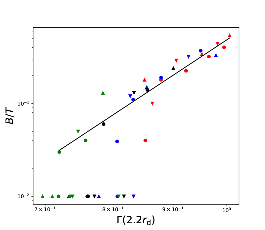
Figure 11: $B/T$ versus the exponent $\Gamma$ of $\Omega(r)$ at $r=2.2r_{\rm d}$. Symbols of the same shape and colour correspond to the same galaxies as in Fig. 7. The black line is a log-log linear least-square fit to the symbols with $B/T>0.01$.

We cannot comment on the long-term evolution of our galaxies because we have not run any simulations for more than $3\,$Gyr and since our resolution is lower than that of Fujii et al. (2018) anyway (the originality of our study is rather in our systematic exploration of the parameter space). However, we have verifed that our discs evolved very little in the last gigayear before we stopped following them, in agreement with Debattista et al. (2017) and Martinez-Valpuesta et al. (2017), who find that the bar strength grows slowly after the initial rapid growth and the formation of a pseudobulge in the first $2\,$Gyr. Furthermore, any result for isolated discs is purely academical when used to discuss the evolution of galaxies on timescales comparable to the Hubble time.

In relation to the second claim, our simulations confirm that $B/T$ and $\Gamma(2.2r_{\rm d})$ are tightly related (Fig. 11). However, we do not consider that $\Gamma$ adds substantial information with respect to $f_{\rm d}$ and the reason is simple. $\Gamma(r)$ is directly linked to the form of the rotation curve ($\Gamma<1$ for a rising rotation curve; $\Gamma>1$ for a declining one), which is the sum in quadrature of $v_{\rm d}$ and $v_{\rm h}$. Substituting Eq. (4) into Eq. (38) gives:

$$\Gamma(r)=1-\beta_{\rm d}f_{\rm d}-\beta_{\rm h}(1-f_{\rm d}),$$ (39)

where:

$$\beta_{\rm d}={{\rm d\,ln}v_{\rm d}\over{\rm d\,ln}r}$$ (40)

and:

$$\beta_{\rm h}={{\rm d\,ln}v_{\rm h}\over{\rm d\,ln}r}={1\over 2}\left({{\rm d\,ln}m_{\rm DM}\over{\rm d\,ln}r}-1\right).$$ (41)

At $r=2.2r_{\rm d}$, $v_{\rm d}$ has a maximum, so that $\beta_{\rm d}(2.2r_{\rm d})=0$; $\beta_{\rm h}(2.2r_{\rm d})$ depends on $cr_{\rm d}$, but, for reasonable values of $c$ and $r_{\rm d}$, its value is always $\beta_{\rm h}(2.2r_{\rm d})\simeq 0.4$ ($\pm 0.1$ at most). In contrast, $f_{\rm d}$ can vary by an order of magnitude from one galaxy to another. Hence, it is $f_{\rm d}$ that determines $\Gamma$, as we intended to demonstrate.

Studies such as those by Athanassoula (2008) and Fujii et al. (2018) show that the formation of a bar is sensitive to the instability threshold $\alpha$ and that $\alpha$ is not universal but depends on parameters that our crude assumption of a static spherical halo cannot capture. However, predicting the stability of individual galaxies with the highest possible accuracy is not the goal of our article. Our goal is to develop a model that may be able to make statistical predictions for the most likely $B/T$ ratios of galaxies given the halo masses, spins, concentrations, and merging histories measured in cosmological N-body simulations.

Considering the quantitative dependence of $B/T$ on $v_{\rm d}/v_{\rm c}$ helps to overcome the problem highlighted by the above studies. We may erroneously predict the formation of a pseudobulge in a galaxy with $v_{\rm d}/v_{\rm c}>\alpha$ that should not have formed one in reality. However, if $v_{\rm d}/v_{\rm c}$ is small, $B/T$ will be small, and galaxies with $B/T<0.1$ are, for many practical purposes, indistinguishable from galaxies with $B/T=0$, particularly when one considers the difficulty of obtaining accurate quantitative morphologies from observations at high redshift. In the same way, our criterion may fail to predict the formation of a pseudobulge in a galaxy with $v_{\rm d}/v_{\rm c}<\alpha$ that should develop one. However, the bulges that we miss are usually small. The clearest example is galaxy md0.3mb1 of Fujii et al. (2018). For that galaxy, the left-hand side of Eq. (1) is equal to $1.87$, so the galaxy should be stable. The simulations by Fujii et al. (2018) show that it is not. However, visual inspection of the morphology after 5 Gyr does not show any massive bulge.

The assumptions under which we have derived Eq. (19) are consistent with the spirit of the semi-analytic approximation, which is to separate the evolution of the DM from that of the baryons within haloes. Cosmological hydrodynamic simulations have shown that baryonic physics can affect the structural properties of DM haloes (Pontzen & Governato, 2012; Teyssier et al., 2013; Di Cintio et al., 2014; Tollet et al., 2016) and cause them to deviate from the NFW profile that SAMs assume, when they do not make the even cruder approximation of a singular isothermal sphere. Using Eq. (19) to assign morphologies to galaxies that have not experienced any mergers is no greater approximation than to model the DM with an NFW profile or to assume that major mergers transform discs into spheroids instantaneously. In fact, Robertson et al. (2006), Hopkins et al. (2009), and Hammer et al. (2009) have shown examples of discs that survived gas-rich major mergers. Yet, a lot has been learned about the Universe from this simple picture.

Finally, despite their simplifying assumptions, our simulations reproduce the magnitude – morphology relation observed in the catalogues from Mathewson et al. (1992), Simard et al. (2011), and Salo et al. (2015). SAMs based on our findings are in very good agreement with the $B/T$ – $M_{*}$ relation (Mendel et al., 2014), especially at $M_{*}\lower 2.15277pt\hbox{$\;\buildrel<\over{\sim}\;$}10^{10}\,M_{\odot}$, where most bulges are pseudobulges formed by disc instabilities in both our SAM and observations. Our results support models in which pseudobulges grow gradually through non-axisymmetric secular disc instabilities as opposed to violent instabilities where discs collapse rapidly into bulges (à la Cole et al., 2000).

We conclude with a note on our future plans. ‘Pseudobulge formation through bar instabilities’ might have been a more precise title for our current article, but we have chosen ‘Bulge formation through disc instabilities’ because we are planning a second article, in which explore how our results can be extended to gas-rich systems. We have seen that a $2\%$ gas fraction increases the final $B/T$ by $\sim 3\%$ on average (Section 4). For high gas fractions, the instability may be not only quantitatively but also qualitatively different. Already Noguchi & Shlosman (1994) found that unstable gas-rich discs do not develop a bar. They fragment into clumps that merge into a central bulge. Bulges formed through this process may be closer to classical bulges than to peanut-shaped pseudobulges (Bournaud et al., 2007). Hence our choice of a title that is broad enough to encompass our future projects.

References

- Abadi et al. (2003) Abadi, M. G., Navarro, J. F., Steinmetz, M., & Eke, V. R. 2003, ApJ, 597, 21
- Anglés-Alcázar et al. (2017) Anglés-Alcázar, D., Faucher-Giguère, C.-A., Kereš, D., et al. 2017, MNRAS, 470, 4698
- Athanassoula (2003) Athanassoula, E. 2003, MNRAS, 341, 1179
- Athanassoula (2005) Athanassoula, E. 2005, MNRAS, 358, 1477
- Athanassoula (2008) Athanassoula, E. 2008, MNRAS, 390, L69
- Athanassoula & Misiriotis (2002) Athanassoula, E. & Misiriotis, A. 2002, MNRAS, 330, 35
- Aubert et al. (2004) Aubert, D., Pichon, C., & Colombi, S. 2004, MNRAS, 352, 376
- Barnes (1992) Barnes, J. E. 1992, ApJ, 393, 484
- Barnes & Hernquist (1991) Barnes, J. E. & Hernquist, L. E. 1991, ApJ, 370, L65
- Baugh et al. (1996) Baugh, C. M., Cole, S., & Frenk, C. S. 1996, MNRAS, 283, 1361
- Behroozi et al. (2019) Behroozi, P., Wechsler, R. H., Hearin, A. P., & Conroy, C. 2019, MNRAS, 488, 3143
- Behroozi et al. (2013) Behroozi, P. S., Wechsler, R. H., & Conroy, C. 2013, ApJ, 770, 57
- Benson (2012) Benson, A. J. 2012, New Astronomy, 17, 175
- Berentzen et al. (1998) Berentzen, I., Heller, C. H., Shlosman, I., & Fricke, K. J. 1998, MNRAS, 300, 49
- Binney & Tremaine (2008) Binney, J. & Tremaine, S. 2008, Galactic Dynamics: Second Edition (Galactic Dynamics: Second Edition, by James Binney and Scott Tremaine. ISBN 978-0-691-13026-2 (HB). Published by Princeton University Press, Princeton, NJ USA, 2008.)
- Bissantz & Gerhard (2002) Bissantz, N. & Gerhard, O. 2002, MNRAS, 330, 591
- Bland-Hawthorn & Gerhard (2016) Bland-Hawthorn, J. & Gerhard, O. 2016, ARA&A, 54, 529
- Boselli et al. (2014) Boselli, A., Cortese, L., Boquien, M., et al. 2014, A&A, 564, A66
- Bournaud et al. (2007) Bournaud, F., Elmegreen, B. G., & Elmegreen, D. M. 2007, ApJ, 670, 237
- Bournaud et al. (2009) Bournaud, F., Elmegreen, B. G., & Martig, M. 2009, ApJ, 707, L1
- Bovy & Rix (2013) Bovy, J. & Rix, H.-W. 2013, ApJ, 779, 115
- Brook et al. (2004) Brook, C. B., Kawata, D., Gibson, B. K., & Freeman, K. C. 2004, ApJ, 612, 894
- Brook et al. (2012) Brook, C. B., Stinson, G., Gibson, B. K., Wadsley, J., & Quinn, T. 2012, MNRAS, 424, 1275
- Bryan et al. (2013) Bryan, S. E., Kay, S. T., Duffy, A. R., et al. 2013, MNRAS, 429, 3316
- Bullock et al. (2001) Bullock, J. S., Dekel, A., Kolatt, T. S., et al. 2001, ApJ, 555, 240
- Burkert et al. (2016) Burkert, A., Förster Schreiber, N. M., Genzel, R., et al. 2016, ApJ, 826, 214
- Cacciato et al. (2012) Cacciato, M., Dekel, A., & Genel, S. 2012, MNRAS, 421, 818
- Carollo et al. (1998) Carollo, C. M., Stiavelli, M., & Mack, J. 1998, AJ, 116, 68
- Cattaneo et al. (2017) Cattaneo, A., Blaizot, J., Devriendt, J. E. G., et al. 2017, MNRAS, 471, 1401
- Cattaneo et al. (2011) Cattaneo, A., Mamon, G. A., Warnick, K., & Knebe, A. 2011, A&A, 533, A5
- Chilingarian et al. (2010) Chilingarian, I. V., Di Matteo, P., Combes, F., Melchior, A. L., & Semelin, B. 2010, A&A, 518, A61
- Christodoulou et al. (1995) Christodoulou, D. M., Shlosman, I., & Tohline, J. E. 1995, ApJ, 443, 551
- Cole et al. (2000) Cole, S., Lacey, C. G., Baugh, C. M., & Frenk, C. S. 2000, MNRAS, 319, 168
- Combes et al. (1990) Combes, F., Debbasch, F., Friedli, D., & Pfenniger, D. 1990, A&A, 233, 82
- Combes et al. (2013) Combes, F., García-Burillo, S., Braine, J., et al. 2013, A&A, 550, A41
- Combes & Sanders (1981) Combes, F. & Sanders, R. H. 1981, A&A, 96, 164
- Comerón et al. (2011) Comerón, S., Elmegreen, B. G., Knapen, J. H., et al. 2011, ApJ, 741, 28
- Croton et al. (2016) Croton, D. J., Stevens, A. R. H., Tonini, C., et al. 2016, ApJS, 222, 22
- de Vaucouleurs et al. (1976) de Vaucouleurs, G., de Vaucouleurs, A., & Corwin, J. R. 1976, in Second reference catalogue of bright galaxies, Vol. 1976, p. Austin: University of Texas Press., Vol. 1976
- Debattista et al. (2017) Debattista, V. P., Ness, M., Gonzalez, O. A., et al. 2017, MNRAS, 469, 1587
- Dekel & Silk (1986) Dekel, A. & Silk, J. 1986, ApJ, 303, 39
- Di Cintio et al. (2014) Di Cintio, A., Brook, C. B., Macciò, A. V., et al. 2014, MNRAS, 437, 415
- Dimauro et al. (2018) Dimauro, P., Huertas-Company, M., Daddi, E., et al. 2018, MNRAS, 478, 5410
- D’Onghia (2015) D’Onghia, E. 2015, ApJ, 808, L8
- Dutton & Macciò (2014) Dutton, A. A. & Macciò, A. V. 2014, MNRAS, 441, 3359
- Efstathiou (2000) Efstathiou, G. 2000, MNRAS, 317, 697
- Efstathiou et al. (1982) Efstathiou, G., Lake, G., & Negroponte, J. 1982, MNRAS, 199, 1069
- Eliche-Moral et al. (2012) Eliche-Moral, M. C., González-García, A. C., Aguerri, J. A. L., et al. 2012, A&A, 547, A48
- Eliche-Moral et al. (2018) Eliche-Moral, M. C., Rodríguez-Pérez, C., Borlaff, A., Querejeta, M., & Tapia, T. 2018, A&A, 617, A113
- Erwin (2018) Erwin, P. 2018, MNRAS, 474, 5372
- Erwin (2019) Erwin, P. 2019, MNRAS, 489, 3553
- Fall & Efstathiou (1980) Fall, S. M. & Efstathiou, G. 1980, MNRAS, 193, 189
- Fisher & Drory (2008) Fisher, D. B. & Drory, N. 2008, AJ, 136, 773
- Fisher & Drory (2011) Fisher, D. B. & Drory, N. 2011, ApJ, 733, L47
- Freeman (1970) Freeman, K. C. 1970, ApJ, 160, 811
- Fujii et al. (2011) Fujii, M. S., Baba, J., Saitoh, T. R., et al. 2011, ApJ, 730, 109
- Fujii et al. (2018) Fujii, M. S., Bédorf, J., Baba, J., & Portegies Zwart, S. 2018, MNRAS, 477, 1451
- Gadotti (2009) Gadotti, D. A. 2009, MNRAS, 393, 1531
- Gargiulo et al. (2015) Gargiulo, I. D., Cora, S. A., Padilla, N. D., et al. 2015, MNRAS, 446, 3820
- Gonzalez-Perez et al. (2014) Gonzalez-Perez, V., Lacey, C. G., Baugh, C. M., et al. 2014, MNRAS, 439, 264
- Graham & Worley (2008) Graham, A. W. & Worley, C. C. 2008, MNRAS, 388, 1708
- Hammer et al. (2009) Hammer, F., Flores, H., Puech, M., et al. 2009, A&A, 507, 1313
- Hammer et al. (2018) Hammer, F., Yang, Y. B., Wang, J. L., et al. 2018, MNRAS, 475, 2754
- Hatton et al. (2003) Hatton, S., Devriendt, J. E. G., Ninin, S., et al. 2003, MNRAS, 343, 75
- Henriques et al. (2015) Henriques, B. M. B., White, S. D. M., Thomas, P. A., et al. 2015, MNRAS, 451, 2663
- Hockney & Hohl (1969) Hockney, R. W. & Hohl, F. 1969, AJ, 74, 1102
- Hohl (1971) Hohl, F. 1971, ApJ, 168, 343
- Hopkins et al. (2009) Hopkins, P. F., Cox, T. J., Younger, J. D., & Hernquist, L. 2009, ApJ, 691, 1168
- Hubble (1926) Hubble, E. P. 1926, ApJ, 64, 321
- Jiang et al. (2019) Jiang, F., Dekel, A., Kneller, O., et al. 2019, MNRAS, 488, 4801
- Jurić et al. (2008) Jurić, M., Ivezić, Ž., Brooks, A., et al. 2008, ApJ, 673, 864
- Kalnajs (1972) Kalnajs, A. J. 1972, ApJ, 175, 63
- Kauffmann et al. (1993) Kauffmann, G., White, S. D. M., & Guiderdoni, B. 1993, MNRAS, 264, 201
- Kimm et al. (2011) Kimm, T., Devriendt, J., Slyz, A., et al. 2011, ArXiv e-prints [arXiv:1106.0538]
- Kormendy (1982) Kormendy, J. 1982, ApJ, 257, 75
- Kormendy (1993) Kormendy, J. 1993, in IAU Symposium, Vol. 153, Galactic Bulges, ed. H. Dejonghe & H. J. Habing, 209
- Kormendy et al. (2010) Kormendy, J., Drory, N., Bender, R., & Cornell, M. E. 2010, ApJ, 723, 54
- Kormendy et al. (2009) Kormendy, J., Fisher, D. B., Cornell, M. E., & Bender, R. 2009, ApJS, 182, 216
- Kormendy & Kennicutt (2004) Kormendy, J. & Kennicutt, Robert C., J. 2004, ARA&A, 42, 603
- Koutsouridou & Cattaneo (2019) Koutsouridou, I. & Cattaneo, A. 2019, MNRAS, 490, 5375
- Leauthaud et al. (2012) Leauthaud, A., Tinker, J., Bundy, K., et al. 2012, ApJ, 744, 159
- Lee & Yi (2013) Lee, J. & Yi, S. K. 2013, ApJ, 766, 38
- Libeskind et al. (2010) Libeskind, N. I., Yepes, G., Knebe, A., et al. 2010, MNRAS, 401, 1889
- Lo Faro et al. (2009) Lo Faro, B., Monaco, P., Vanzella, E., et al. 2009, MNRAS, 399, 827
- Macciò et al. (2012) Macciò, A. V., Stinson, G., Brook, C. B., et al. 2012, ApJ, 744, L9
- Martinez-Valpuesta et al. (2017) Martinez-Valpuesta, I., Aguerri, J. A. L., González-García, A. C., Dalla Vecchia, C., & Stringer, M. 2017, MNRAS, 464, 1502
- Mathewson et al. (1992) Mathewson, D. S., Ford, V. L., & Buchhorn, M. 1992, ApJS, 81, 413
- Meert et al. (2015) Meert, A., Vikram, V., & Bernardi, M. 2015, MNRAS, 446, 3943
- Meert et al. (2016) Meert, A., Vikram, V., & Bernardi, M. 2016, MNRAS, 455, 2440
- Mendel et al. (2014) Mendel, J. T., Simard, L., Palmer, M., Ellison, S. L., & Patton, D. R. 2014, ApJS, 210, 3
- Mo et al. (1998) Mo, H. J., Mao, S., & White, S. D. M. 1998, MNRAS, 295, 319
- Moster et al. (2013) Moster, B. P., Naab, T., & White, S. D. M. 2013, MNRAS, 428, 3121
- Moster et al. (2018) Moster, B. P., Naab, T., & White, S. D. M. 2018, MNRAS, 477, 1822