A theoretical framework of BL Her stars. I. Effect of metallicity and convection parameters on period-luminosity and period-radius relations

Abstract

We present a new grid of convective BL Herculis models using the state-of-the-art 1D non-linear radial stellar pulsation tool mesa-rsp. We investigate the impact of metallicity and four sets of different convection parameters on multi-wavelength properties. Non-linear models were computed for periods typical for BL Her stars, i.e. $1\leq\mathrm{P(days)}\leq 4$ covering a wide range of input parameters - metallicity ($-2.0\;\mathrm{dex}\leq\mathrm{[Fe/H]}\leq 0.0\;\mathrm{dex}$), stellar mass (0.5M_⊙-0.8M_⊙), luminosity (50L_⊙-300L_⊙) and effective temperature (full extent of the instability strip; in steps of 50K). The total number of BL Her models with full-amplitude stable pulsations used in this study is 10280 across the four sets of convection parameters. We obtain their multiband ($UBVRIJHKLL^{\prime}M$) light curves and derive new theoretical period-luminosity ($PL$), period-Wesenheit ($PW$) and period-radius ($PR$) relations at mean light. We find that the models computed with radiative cooling show statistically similar slopes for $PL$, $PW$ and $PR$ relations. Most empirical relations match well with the theoretical $PL$, $PW$ and $PR$ relations from the BL Her models computed using the four sets of convection parameters. However, $PL$ slopes of the models with radiative cooling provide a better match to empirical relations for BL Her stars in the LMC in the $HK_{S}$ bands. For each set of convection parameters, the effect of metallicity is significant in $U$ and $B$-bands and negligible in infrared bands, which is consistent with empirical results. No significant metallicity effects are seen in the $PR$ relations.

1 Introduction

Type II Cepheids (T2Cs) are pulsating stars located in the instability strip of the Hertzsprung-Russell diagram (HRD). T2Cs are brighter than the RR Lyrae stars but fainter than the classical Cepheids. Based on their pulsational period, T2Cs are divided into the following subclasses: the BL Herculis (BL Her: $1\lesssim P\textrm{(days)}\lesssim 4$), the W Virginis (W Vir: $4\lesssim P\textrm{(days)}\lesssim 20$) and the RV Tauris (RV Tau: $P\gtrsim 20$ days) (Soszyński et al., 2018). However, the period separation for different subclasses is not strict, for example, the upper limit on the period of BL Her stars is set at 4 days in the Magellanic Clouds Soszyński et al. (2018) and 5 days in the Galactic bulge Soszyński et al. (2017). Similar to RR Lyrae stars and classical Cepheids, T2Cs follow well-defined period-luminosity ($PL$) relationships (Matsunaga et al., 2006; Groenewegen et al., 2008; Matsunaga et al., 2009; Ciechanowska et al., 2010; Matsunaga et al., 2011; Ripepi et al., 2015; Bhardwaj et al., 2017a; Bhardwaj et al., 2017b; Groenewegen & Jurkovic, 2017b; Braga et al., 2018), which makes them useful distance indicators (see reviews, Beaton et al., 2018; Bhardwaj, 2020).

T2Cs are population II stars and trace low mass, metal-poor, old-age stellar populations. However, recent studies suggest that W Vir stars may have their origin in binary systems (Groenewegen & Jurkovic, 2017a) and that RV Tau stars may also have massive and younger progenitors (Manick et al., 2018). T2Cs have a wide range of metallicities (Welch, 2012). While Clement et al. (2001) noted that all the Galactic Globular Clusters (GGCs) containing T2Cs have $\mathrm{[Fe/H]}<-1.0$ dex, Galactic field T2Cs were found to have metallicities in the range $-1.0\;\mathrm{dex}<\mathrm{[Fe/H]}<0\;\mathrm{dex}$ (Schmidt et al., 2011). T2Cs in the Bulge have photometric metallicities ranging from $-1.4$ dex to $+0.6$ dex, with $\mathrm{[Fe/H]_{mean}}=-0.6\pm 0.17$ dex (Harris & Wallerstein, 1984; Wallerstein, 2002). In a recent study to understand the origin of the Galactic Halo, Wallerstein & Farrell (2018) found $\mathrm{[Fe/H]}>-0.9$ dex for a majority of the field T2Cs. We therefore adopt a broad range of metallicities, $-2\;\mathrm{dex}<\mathrm{[Fe/H]}<0\;\mathrm{dex}$ for computing BL Her models in the present study.

Empirical $PL$ relations of T2Cs have been studied extensively in the last few decades. Nemec et al. (1994) provided $P-L-\mathrm{[Fe/H]}$ relations for T2Cs in the GGCs in the optical $BV$ bands. Matsunaga et al. (2006) did not find any significant metallicity effect on the $PL$ relations in their study of $PL$ relations using 46 T2Cs in 26 GGCs; the observations were obtained from the Infrared Survey Facility (IRSF) 1.4-m telescope in the near-infrared $JHK_{S}$ bands. Using 39 T2Cs in the Galactic Bulge monitored with the SOFI infrared camera on the 3.5-m NTT on ESO/La Silla, Groenewegen et al. (2008) provided $PL$ relations in the $K$-band and estimated a distance modulus of $14.51\pm 0.12\pm 0.07$ (systematic) mag to the Galactic Centre. The $PL$ relations for Galactic T2Cs in the Gaia $G$-band have been provided by Clementini et al. (2016). In a series of papers, Matsunaga et al. (2009, 2011) presented near-infrared ($JHK_{S}$) $PL$ and Wesenheit relations for T2Cs in the Large (LMC) and Small (SMC) Magellanic Clouds obtained using data from IRSF and SIRIUS. Near-infrared $PL$ and period-Wesenheit ($PW$) relations for T2Cs in the LMC have been presented by Ripepi et al. (2015) using the VISTA Magellanic Cloud survey (VMC, Cioni et al., 2011) and by Bhardwaj et al. (2017a) using observations obtained by the Large Magellanic Cloud Near-infrared Synoptic Survey (LMCNISS, Macri et al., 2015). Recently, Manick et al. (2017) published $PW$ relations for T2Cs in the LMC using the Optical Gravitational Lensing Experiment (OGLE-III, Soszyński et al., 2008) data, while Groenewegen & Jurkovic (2017b) presented $PL$ relations of the Magellanic Cloud T2Cs based on OGLE-III data reporting no dependence on metallicity.

Burki & Meylan (1986) and Balog et al. (1997) are few of the earlier studies where the empirical period-radius ($PR$) relations of T2Cs were investigated. A detailed study of the $PR$ relations of T2Cs in the Magellanic Clouds has been carried out by Groenewegen & Jurkovic (2017b) based on OGLE-III data. They found the $PR$ relations to have little or no dependence on metallicity.

On the theoretical front, several linear and non-linear convective T2C models, in particular, BL Her models have been computed by Bono et al. (1995); Bono et al. (1997a); Bono et al. (1997b); Marconi & Di Criscienzo (2007); Smolec et al. (2012); Smolec & Moskalik (2012, 2014); Smolec (2016). Buchler & Moskalik (1992) had predicted period doubling in BL Her stars which is caused by the 3:2 resonance between the fundamental mode and the first overtone. This was confirmed almost 20 years later when the period doubling behaviour was observed in a 2.4-d BL Her type variable in the Galactic bulge and consistently modeled with the observed light curves (Soszyński et al., 2011; Smolec et al., 2012). Few theoretical studies have provided $PL$ and $PR$ relations for BL Her models. Theoretical near-infrared period-magnitude and $PW$ relations for BL Her models in the metal abundance range of $Z=0.0001$ to $Z=0.004$ were derived by Di Criscienzo et al. (2007) while Marconi & Di Criscienzo (2007) presented theoretical $PR$ relation for BL Her models and found it to be in excellent agreement with the empirical relation from Burki & Meylan (1986).

The recently released non-linear Radial Stellar Pulsation (rsp) tool in Modules for Experiments in Stellar Astrophysics (mesa, Paxton et al., 2011; Paxton et al., 2013, 2015, 2018, 2019) may be used for generating multi-wavelength light curves of classical pulsators. Along with being an open-source code, mesa-rsp offers the advantage of testing how properties of the models depend on the details of convection model used, by varying convective parameters. Das et al. (2020) computed a few RR Lyrae, BL Her and classical Cepheid models using mesa-rsp and found the theoretical period-colour (PC) relations to be in good agreement with the empirical PC relations. The aim of this project is to compute a very fine grid of BL Her models, encompassing a wide range of metallicity, mass, luminosity and effective temperature using the most recent, state-of-the-art stellar pulsation code, the mesa-rsp. We also obtain theoretical $PL$ and $PR$ relations for these stars and test the effect of convection parameters and metallicity on these relations. The reason for choosing BL Her stars only (and not the other subclasses of T2Cs) for our study is two-fold: (i) Matsunaga et al. (2011) found evidence that $PL$ relations of BL Her and W Vir stars should be discussed independently (ii) The highly non-adiabatic longer-period T2Cs (W Vir and RV Tau stars) pose problems for the existing pulsation codes and are current limitations of mesa-rsp (Smolec, 2016; Paxton et al., 2019). However, mesa-rsp may be reliably used for modelling the shortest-period class of T2Cs, the BL Her stars.

The structure of this paper is as follows: The BL Her models computed using mesa-rsp are described in Section 2. In Sections 3 and 4, we study the $PL$ and $PR$ relations of these models and investigate any possible dependence of these relations on metallicity and convection parameters. Finally, we summarise the results of this study in Section 6.

2 The stellar pulsation models

Since mesa-rsp offers the possibility of using different convection parameter sets, we explore the effect of different convection parameters on the multi-wavelength $PL$ and $PR$ relations of a finely computed grid of BL Her models. We note here that mesa-rsp uses the theory of turbulent convection as outlined in Kuhfuss (1986) and follows Smolec & Moskalik (2008) in its treatment of stellar pulsation. The free parameters that enter the convective model are provided in Tables 3 and 4 of Paxton et al. (2019). For convenience, they are listed in Table 1. Set A corresponds to the simplest convection model, set B adds radiative cooling, set C adds turbulent pressure and turbulent flux, and set D includes these effects simultaneously. A detailed description of the free parameters and their standard values is provided in Smolec & Moskalik (2008). In brief, parameters $\alpha_{p}$ and $\alpha_{c}$ were introduced by Yecko et al. (1998) and their values were set at $\alpha_{p}$=2/3 and $\alpha_{c}$=$\alpha_{s}$. The value for $\gamma_{r}$=$2\sqrt{3}$ is obtained from Wuchterl & Feuchtinger (1998). Neglecting radiative cooling and turbulent pressure reduces the time-independent version of the convection model (Kuhfuss, 1986) to the standard mixing-length theory (MLT), provided the values for $\alpha_{s}$, $\alpha_{c}$ and $\alpha_{d}$ are kept the same as in Table 1. Paxton et al. (2019) suggest $\alpha_{t}\simeq 0.01$, $\alpha_{m}\lesssim 1$, and $\alpha\lesssim 2$ as useful starting choices. We stress here that we have not made any changes to the free parameters in this work and have used the four sets of convection parameters as provided in Paxton et al. (2019). We use mesa r$11701$ for our present study. OPAL opacity tables (Iglesias & Rogers, 1996) supplemented at low temperatures with Ferguson et al. (2005) opacity data were adopted.

Table 1: The free parameters and their associated values in the convective parameter sets A, B, C and D of the mesa-rsp convection model.

Name	Parameter description	Set A	Set B	Set C	Set D
$\alpha$	Mixing-length parameter	1.5	1.5	1.5	1.5
$\alpha_{m}$	Eddy-viscous dissipation parameter	0.25	0.50	0.40	0.70
$\alpha_{s}$	Turbulent source parameter	$\frac{1}{2}\sqrt{\frac{2}{3}}$	$\frac{1}{2}\sqrt{\frac{2}{3}}$	$\frac{1}{2}\sqrt{\frac{2}{3}}$	$\frac{1}{2}\sqrt{\frac{2}{3}}$
$\alpha_{c}$	Convective flux parameter	$\frac{1}{2}\sqrt{\frac{2}{3}}$	$\frac{1}{2}\sqrt{\frac{2}{3}}$	$\frac{1}{2}\sqrt{\frac{2}{3}}$	$\frac{1}{2}\sqrt{\frac{2}{3}}$
$\alpha_{d}$	Turbulent dissipation parameter	$\frac{8}{3}\sqrt{\frac{2}{3}}$	$\frac{8}{3}\sqrt{\frac{2}{3}}$	$\frac{8}{3}\sqrt{\frac{2}{3}}$	$\frac{8}{3}\sqrt{\frac{2}{3}}$
$\alpha_{p}$	Turbulent pressure parameter	0	0	$\frac{2}{3}$	$\frac{2}{3}$
$\alpha_{t}$	Turbulent flux parameter	0	0	0.01	0.01
$\gamma_{r}$	Radiative cooling parameter	0	$2\sqrt{3}$	0	$2\sqrt{3}$

2.1 Linear computations

We compute a fine grid of BL Her models for each of the four convection sets with the following input parameters:

1. Metallicity (Corresponding $ZX$ values are provided in Table 2)
   

   $\mathrm{[Fe/H]\;\mathrm{(in\;dex)}}=-2,-1.5,-1.35,-1,-0.5,-0.2,0$
   

   Table 2: Chemical compositions of the adopted pulsation models^∗.

   [Fe/H]	$Z$	$X$
   -2.00	0.00014	0.75115
   -1.50	0.00043	0.75041
   -1.35	0.00061	0.74996
   -1.00	0.00135	0.74806
   -0.50	0.00424	0.74073
   -0.20	0.00834	0.73032
   0.00	0.01300	0.71847

   • ^∗ The $Z$ and $X$ values are estimated from the $\mathrm{[Fe/H]}$ values by assuming the primordial helium value of 0.2485 from the WMAP CMB observations (Hinshaw et al., 2013) and the helium enrichment parameter value of 1.54 (Asplund et al., 2009). The solar mixture is adopted from Asplund et al. (2009).

2. Stellar mass ($M$)

   1. Low-mass range = 0.5M_⊙, 0.55M_⊙, 0.6M_⊙

   2. High-mass range = 0.65M_⊙, 0.7M_⊙, 0.75M_⊙, 0.8M_⊙

3. Stellar luminosity ($L$)

   1. For low-mass range = 50L_⊙ to 200L_⊙, in steps of 50L_⊙

   2. For high-mass range = 50L_⊙ to 300L_⊙, in steps of 50L_⊙

4. Effective temperature ($T_{\rm{eff}}$) = 4000K to 8000K, in steps of 50K.

This results in a combination of 20412 models per convective parameter set. BL Her stars belong to the low-mass population with masses $\sim 0.5M_{\odot}-0.6M_{\odot}$ (Bhardwaj, 2020). However, we also explore the possibility of higher mass BL Her stars in this study. In his survey of non-linear convective T2C models, Smolec (2016) computed a grid using $0.6M_{\odot}$ and $0.8M_{\odot}$. The effective temperature range chosen in the present study is much broader than the actual width of the instability strip to accurately estimate the edges of the instability strip. mesa-rsp may be used to compute models where the structure of the stellar envelope determines the pulsations (Paxton et al., 2019), without taking into consideration the detailed structure of the core. We begin with a computation of linear properties of the models with the same method as described in Smolec (2016) and Paxton et al. (2019). To this end, equilibrium static models are constructed with $ZXMLT_{\rm{eff}}$ as the input stellar parameters and their linear stability analysis is conducted, which yields linear periods of the radial pulsation modes and their growth rates. The latter may be used to delineate the boundaries of the instability strip. The static models also serve as input for non-linear model integration. Fig. 1 shows the HRD of the grid of computed BL Her models with the convection parameter set A, showing the edges of the instability strip and the lines of constant fundamental mode period (linear value) equal to 1 and 4 days. The other convective parameter sets (B, C and D) show similar HRDs. A future paper will investigate linear results in greater detail.

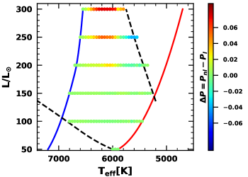
Figure 1: The Hertzsprung-Russell diagram of the grid of computed BL Her models with the convection parameter set A. The edges of the instability strip are estimated from the linear stability analysis and are shown with the blue and red solid lines. The dashed lines are lines of constant fundamental mode period (linear value) equal to 1 day (bottom) and 4 days (top). The dots represent the BL Her models used in this analysis while the colourbar shows the difference between the non-linear and linear period of the computed models, i.e., $\Delta P=P_{nl}-P_{l}$. The mean difference between the linear and non-linear periods in our models is $\sim$0.02 days.

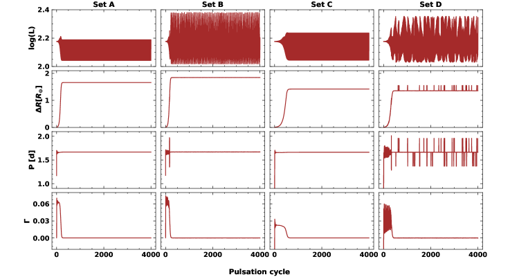
Figure 2: Luminosity $\log(L)$, amplitude of radius variation $\Delta R$, period $P$ and fractional growth rate $\Gamma$ during 4000-cycle integrations of the BL Her model with input parameters, $Z=0.013$, $X=0.71847$, $M=0.7$M_⊙, $L=150$L_⊙, $T=6350$K. The models with the same input parameters computed using sets A, B and C satisfy the condition of full-amplitude stable pulsation ($\Delta R$, $P$ and $\Gamma$ do not vary by more than 0.01 over the last $\sim$100-cycles of the total 4000-cycle integrations) and are accepted for the analysis while the model computed using Set D is rejected.

2.2 Non-Linear computations

We proceed with the non-linear computations for models that have positive growth rates of the radial fundamental mode and linear periods between 0.8 and 4.2 days. The period range is larger than considered for BL Her stars due to non-linear period changes. While non-linear period shifts expected for BL Her models are well below 0.05 days (see Fig. 6 in Smolec, 2016), the changes of up to 0.2 days are noted for more luminous type II Cepheid models. Finally, we only select models with non-linear periods between 1 and 4 days as BL Her models, considering the typical period range of BL Her stars (Soszyński et al., 2018). We also confirm that non-linear period shifts are below 0.09 days in our models, with a mean non-linear period shift of $\sim$0.02 days.

Note that the quantities that enter into energy and momentum equations of the mesa-rsp convection model depend on the free parameters described in Table 1; Paxton et al. (2019) found that the pulsation periods of the models weakly depend on the values of these free parameters. Therefore, a model with the same input parameters $ZXMLT_{\rm{eff}}$ may have different non-linear periods across the different sets of convection parameters.

The non-linear model integration is carried for 4000 pulsation cycles; the control used for this terminating condition is RSP_max_num_periods in mesa-rsp. It is essential to check for full-amplitude stable pulsations of the models before obtaining the theoretical $PL$ and $PR$ relations. The model reaches full amplitude pulsation state when its kinetic energy per pulsation period remains constant. We can quantify that using the fractional growth of the kinetic energy per pulsation period $\Gamma$ which should approach zero once stable pulsation state is reached. These pulsations may show some irregularities, e.g. period doubling effect or chaotic oscillations (Smolec et al., 2012; Smolec & Moskalik, 2012, 2014). Since we are interested in stable single periodic oscillation, we also investigate whether the amplitude of radius variation $\Delta R$ and the pulsation period $P$ computed on a cycle to cycle basis is stable. For our study, the condition of full-amplitude stable pulsation is satisfied and the model is accepted when its $\Delta R$, $P$ and $\Gamma$ do not vary by more than 0.01 over the last $\sim$100-cycles of the total 4000-cycle integrations, failing which the model is rejected from further analysis. Fig. 2 shows an example for one particular model- while sets A, B and C exhibit full-amplitude stable pulsations and are accepted, the set D model is most likely chaotic and is rejected from our analysis. The number of models accepted in sets B and D is much less than in sets A and C. The sets B and D include radiative cooling with the parameter $\gamma_{r}=2\sqrt{3}$, while this parameter is set to zero in the sets A and C. Table 3 summarises the number of BL Her models for each convection parameter set.

We note that the higher stellar mass (>0.6$M_{\odot}$) and lower metallicity (Z=0.00014) considered in our work is typical of Zero Age Horizontal Branch or evolved RR Lyrae stars. However, as discussed in Braga et al. (2020), the separation between RR Lyrae and T2Cs is a long-standing problem. A threshold of period $\sim$1 day typically separates the two classes of pulsating variable stars (Soszyński et al., 2008, 2014). Braga et al. (2020) report the star V92 in $\omega$-Cen (with a period of 1.3 days) to be a candidate RR Lyrae star because its core is likely in the helium-burning phase. Given the evidence, it is rather difficult to separate completely unambiguously the two different classes of pulsating variables based on their chemical composition. It might be possible to separate RR Lyrae and BL Her stars based on their evolutionary status, although this is not easily done for field stars. However, in this work, we use the conventional classification for BL Her variables as population II stars with pulsation period between 1 and 4 days (Soszyński et al., 2018).

Table 3: A summary of the number of BL Her models in each convection parameter set finally used in the analysis.

Condition	Set A	Set B	Set C	Set D
Total $ZXMLT_{\rm{eff}}$ combinations	20412	20412	20412	20412
(Models computed in the linear grid)
Models with positive growth rate of the F-mode	4481	4356	4061	4192
and with linear period: $0.8\leq P\leq 4.2$
(Models computed in the non-linear grid)
Models with non-linear period: $1\leq P\leq 4$	4049	3854	3629	3678
Models with full-amplitude stable pulsation†	3266	2260	2632	2122

• ^† Satisfies the condition that the amplitude of radius variation $\Delta R$, period $P$ and fractional growth rate $\Gamma$ do not vary by more than 0.01 over the last $\sim$100-cycles of the total 4000-cycle integrations. For a clear, pictorial representation of full-amplitude stable pulsation, the reader may refer to Fig. 2.

2.3 Processing the data

The details on the transformation of bolometric light curves into optical and NIR bands is given in Paxton et al. (2018) and is briefly summarised here. The luminosity $\rm{\log_{10}(L/L_{\odot})}$ obtained from the non-linear computations of the models is converted to the absolute bolometric magnitude ($\rm{M_{bol}}$) of the model using:

$$\rm{M_{bol}=M_{bol,\odot}-2.5\log_{10}(L/L_{\odot})},$$ (1)

where $\rm{M_{bol,\odot}}=4.74$ (Mamajek et al., 2015) is the absolute bolometric magnitude of the Sun. The absolute bolometric magnitude is then transformed into the absolute magnitude $\rm{M_{\lambda}}$ in a given band $\lambda$ using:

$$\rm{M_{\lambda}=M_{bol}-BC_{\lambda}},$$ (2)

where $\rm{BC_{\lambda}}$ is the bolometric correction for band $\lambda$. mesa provides pre-computed bolometric correction tables where the bolometric correction is defined as a function of the stellar photosphere. For given stellar photosphere parameters, the bolometric correction table is interpolated over $\log(T)$, $\log(g)$ and the metallicity [M/H] within the parameter range of that table. We use the pre-processed table from Lejeune et al. (1998) which provides bolometric corrections over the parameter range $2000\leq T_{\rm{eff}}\rm{(K)}\leq 50,000$, $-1.02\leq\log(g)\rm{(cms^{-2})}\leq 5.0$, and $-5.0\leq[M/H]\leq 1.0$ and for the Johnson-Cousins-Class bands $UBVR_{c}I_{c}JHKLL^{\prime}M$. The minimal impact of adopted transformations on the mean-light properties at wavelengths longer than $V$-band is discussed in Appendix A.

The multi-wavelength theoretical light-curves of the accepted models are fitted with the Fourier sine series (see example, Deb & Singh, 2009; Bhardwaj et al., 2015; Das et al., 2018) of the form:

$$m(x)=m_{0}+\sum_{k=1}^{N}A_{k}\sin(2\pi kx+\phi_{k}),$$ (3)

where $x$ is the pulsation phase, $m_{0}$ is the mean magnitude and $N$ is the order of the fit ($N=20$). Table 4 summarises the input stellar parameters of the BL Her models used in this analysis, alongwith the multi-wavelength absolute mean magnitudes obtained from the Fourier fitting. An example of light-curves for a BL Her model obtained using mesa-rsp over multiple wavelengths is presented in Fig. 3.

Table 4: A summary of the BL Her models used in this analysis computed using mesa-rsp. The columns provide the input parameters ($ZXMLT_{\rm{eff}}$), the convection parameter set used, logarithmic pulsation period, logarithmic radius and the absolute mean magnitudes in the bands $UBVR_{c}I_{c}JHKLL^{\prime}M$ and the bolometric.

$Z$	$X$	$M/M_{\odot}$	$L/L_{\odot}$	$\rm{T_{eff}(K)}$	Convection Set	$\log(P)$	$\log(R)$	$M_{U}$	$M_{B}$	$M_{V}$	$M_{R}$	$M_{I}$	$M_{J}$	$M_{H}$	$M_{K}$	$M_{L}$	$M_{L^{\prime}}$	$M_{M}$	$M_{Bol}$
0.00014	0.75115	0.50	50	5950	A	0.011	0.826	0.971	1.087	0.660	0.350	0.033	-0.412	-0.793	-0.732	-0.867	-0.870	-1.242	0.493
0.00014	0.75115	0.50	100	5650	A	0.367	1.024	0.382	0.452	-0.051	-0.411	-0.774	-1.259	-1.700	-1.627	-1.782	-1.787	-2.223	-0.257
…	…	…	…	…	…	…	…	…	…	…	…	…	…	…	…	…	…	…	…
0.00014	0.75115	0.50	100	5700	B	0.355	1.018	0.351	0.428	-0.060	-0.413	-0.770	-1.246	-1.677	-1.606	-1.757	-1.762	-2.187	-0.258
0.00014	0.75115	0.50	100	5750	B	0.336	1.013	0.342	0.417	-0.064	-0.411	-0.761	-1.230	-1.653	-1.583	-1.733	-1.737	-2.155	-0.256
…	…	…	…	…	…	…	…	…	…	…	…	…	…	…	…	…	…	…	…
0.00014	0.75115	0.50	50	5850	C	0.059	0.857	1.036	1.159	0.689	0.346	-0.003	-0.463	-0.879	-0.813	-0.957	-0.961	-1.370	0.493
0.00014	0.75115	0.50	50	5900	C	0.038	0.848	1.015	1.137	0.681	0.348	0.009	-0.446	-0.850	-0.786	-0.927	-0.931	-1.328	0.493
…	…	…	…	…	…	…	…	…	…	…	…	…	…	…	…	…	…	…	…
0.00014	0.75115	0.50	50	5900	D	0.039	0.848	1.012	1.135	0.680	0.347	0.008	-0.445	-0.849	-0.786	-0.926	-0.930	-1.325	0.493
0.00014	0.75115	0.50	50	5950	D	0.019	0.839	0.994	1.114	0.672	0.349	0.020	-0.430	-0.823	-0.761	-0.899	-0.902	-1.287	0.493
…	…	…	…	…	…	…	…	…	…	…	…	…	…	…	…	…	…	…	…

• Note: This table is available entirely in a machine-readable form in the online journal as supporting information.

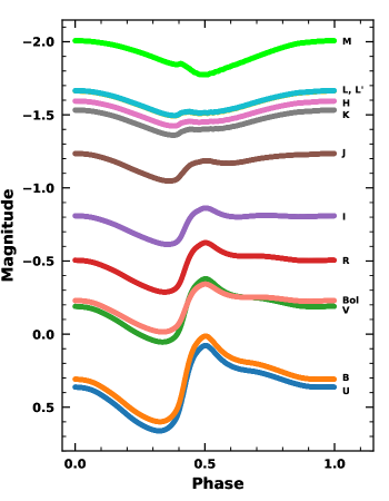
Figure 3: An example of the multi-wavelength light-curves for the BL Her model with input parameters, $Z=0.00424$, $X=0.74073$, $M=0.80$M_⊙, $L=100$L_⊙, $T=6050$K using convective parameter set A.

3 Period-luminosity relations

The mean magnitudes obtained from Fourier fitting of the theoretical light-curves of the BL Her models are used to derive multi-wavelength $PL$ relations of the mathematical form:

$$M_{\lambda}=a\log(P)+b,$$ (4)

where, $M_{\lambda}$ refers to the absolute magnitude in a given band, $\lambda$.

3.1 Effect of convection parameters on $PL$ relations

To study the effect of convection parameters on the $PL$ relations, we use the standard $t$-test to check the statistical equivalence of the slopes from $PL$ relations of the BL Her models obtained using different convective parameter sets. A detailed description of the test is provided in Ngeow et al. (2015) and Das et al. (2020) and is summarised here briefly. The $T$ statistic to compare slopes, $\hat{W}$ of two linear regressions with sample sizes, $n$ and $m$, respectively is defined as:

$$T=\frac{\hat{W}_{n}-\hat{W}_{m}}{\sqrt{\mathrm{Var}(\hat{W}_{n})+\mathrm{Var}(\hat{W}_{m})}},$$ (5)

where $\mathrm{Var}(\hat{W})$ is the variance of the slope. We reject the null hypothesis of equivalent slopes if $T>t_{\alpha/2,\nu}$ or the probability of the observed value of the $T$ statistic is $p<0.05$. $t_{\alpha/2,\nu}$ is the critical value under the two-tailed $t$-distribution with 95% confidence limit ($\alpha$=0.05) and degrees of freedom, $\nu=n+m-4$.

Table 5 lists the statistical comparison of the multi-wavelength $PL$ relation slopes of the BL Her models with respect to literature values. The BL Her models with radiative cooling (sets B and D) exhibit statistically similar $PL$ slopes at any given wavelength, except in the $U$-band while those without radiative cooling (sets A and C) have statistically similar $PL$ slopes only in the $HLL^{\prime}$ bands. BL Her models computed with different convection parameters do show differences in the slopes of the $PL$ relations at a given wavelength. However, most empirical $PL$ relations are consistent with theoretical $PL$ relations based on any set of convection parameter. The $PL$ slopes obtained for the BL Her stars in the Galactic bulge by Bhardwaj et al. (2017b) and in the SMC by Matsunaga et al. (2009) are statistically similar with those obtained from the BL Her models using all four sets of convection parameters and across $JHK_{S}$ bands. Our models in all four convection parameter sets show statistically different $PL$ slopes from the $PL$ slope obtained by Matsunaga et al. (2006) for BL Her stars in the Globular clusters in the $J$-band; however, they exhibit statistically similar $PL$ slopes in the $HK_{S}$ bands. For the BL Her stars in the LMC, $PL$ relations in the $J$-band show similar slopes between empirical data and models using all four sets of convection parameters; however, $PL$ slopes of the models with sets B and D seem to match better with empirical relations in the $HK_{S}$ bands. The bolometric $PL$ relations obtained by Groenewegen & Jurkovic (2017b) for BL Her stars in the Magellanic Clouds show statistically similar slopes with models of different convection parameter sets, except for models computed with set A when the observed BL Her stars in the LMC and the SMC are considered together. The fact that the $PL$ slopes are statistically different between different sets of models, but empirically determined $PL$ slopes are still compatible with all four sets of model $PL$ slopes tells us that the models have lower uncertainty and scatter. Larger and more precise observational datasets are necessary to constrain the best fitting model parameters. From Table 5, we find that the $PL$ slopes from the BL Her models become steeper with increasing wavelengths. This is similar to RR Lyrae as shown empirically in Beaton et al. (2018); Neeley et al. (2017); Bhardwaj et al. (2020). The dispersion in the theoretical $PL$ relations for BL Hers decreases significantly on moving from optical to infrared wavelengths and becomes statistically similar for wavelengths longer than $H$-band. A similar decrease of intrinsic dispersion of the $PL$ relations when changing from the optical to infrared bands has been reported by Neeley et al. (2017) based on RR Lyrae models from Marconi et al. (2015), and is also seen in empirical $PL$ relations of RR Lyrae (e.g. Bhardwaj et al., 2020). This trend in dispersion is expected because of the stronger temperature sensitivity of the bolometric correction in the near-infrared, resulting in brighter magnitudes of BL Hers at cooler effective temperatures (Bono et al., 2003) and a marginal effect of the intrinsic temperature width of the instability strip on the infrared $PL$ relations. In addition, the width of the instability strip itself decreases at longer wavelengths, resulting in smaller dispersion of $PL$ relations (Catelan et al., 2004; Madore & Freedman, 2012; Marconi et al., 2015). We also observe that the models computed using set B have the smallest dispersion in their $PL$ relations in all the bands.

Table 5: Comparison of the slopes of the period-luminosity relations for BL Her stars of the mathematical form $M_{\lambda}=a\log(P)+b$. $N$ is the total number of stars and the number in parentheses indicates the number of outliers. |$T$| represents the observed value of the $t$-statistic, and $p(t)$ gives the probability of acceptance of the null hypothesis (equal slopes). The bold-faced entries indicate that the null hypothesis of the equivalent $PL$ slopes can be rejected.

Band	Source	$a$	$b$	$\sigma$	$N$	Reference‡	Theoretical/ Empirical	(|$T$|, $p(t)$) w.r.t.
								Set A	Set B	Set C	Set D
U	$\rm{Z_{all}}$ (Set A)	-0.841$\pm$0.044	0.185$\pm$0.015	0.391	3266	TW	Theoretical	…	…	…	…
U	$\rm{Z_{all}}$ (Set B)	-0.596$\pm$0.046	0.215$\pm$0.015	0.353	2260	TW	Theoretical	(3.846,0.0)	…	…	…
U	$\rm{Z_{all}}$ (Set C)	-0.422$\pm$0.051	0.298$\pm$0.018	0.428	2632	TW	Theoretical	(6.219,0.0)	(2.512,0.006)	…	…
U	$\rm{Z_{all}}$ (Set D)	-0.369$\pm$0.053	0.309$\pm$0.018	0.409	2122	TW	Theoretical	(6.851,0.0)	(3.213,0.001)	(0.722,0.235)	…
B	$\rm{Z_{all}}$ (Set A)	-1.166$\pm$0.04	0.187$\pm$0.014	0.351	3266	TW	Theoretical	…	…	…	…
B	$\rm{Z_{all}}$ (Set B)	-0.896$\pm$0.041	0.209$\pm$0.013	0.311	2260	TW	Theoretical	(4.764,0.0)	…	…	…
B	$\rm{Z_{all}}$ (Set C)	-0.942$\pm$0.043	0.33$\pm$0.015	0.359	2632	TW	Theoretical	(3.843,0.0)	(0.791,0.214)	…	…
B	$\rm{Z_{all}}$ (Set D)	-0.805$\pm$0.044	0.324$\pm$0.015	0.339	2122	TW	Theoretical	(6.1,0.0)	(1.508,0.066)	(2.235,0.013)	…
V	$\rm{Z_{all}}$ (Set A)	-1.616$\pm$0.032	-0.14$\pm$0.011	0.284	3266	TW	Theoretical	…	…	…	…
V	$\rm{Z_{all}}$ (Set B)	-1.374$\pm$0.034	-0.134$\pm$0.011	0.256	2260	TW	Theoretical	(5.221,0.0)	…	…	…
V	$\rm{Z_{all}}$ (Set C)	-1.487$\pm$0.034	-0.031$\pm$0.012	0.288	2632	TW	Theoretical	(2.761,0.003)	(2.343,0.01)	…	…
V	$\rm{Z_{all}}$ (Set D)	-1.337$\pm$0.036	-0.043$\pm$0.012	0.275	2122	TW	Theoretical	(5.829,0.0)	(0.757,0.225)	(3.023,0.001)	…
R	$\rm{Z_{all}}$ (Set A)	-1.853$\pm$0.028	-0.364$\pm$0.01	0.248	3266	TW	Theoretical	…	…	…	…
R	$\rm{Z_{all}}$ (Set B)	-1.634$\pm$0.03	-0.365$\pm$0.01	0.227	2260	TW	Theoretical	(5.357,0.0)	…	…	…
R	$\rm{Z_{all}}$ (Set C)	-1.739$\pm$0.03	-0.281$\pm$0.01	0.254	2632	TW	Theoretical	(2.774,0.003)	(2.463,0.007)	…	…
R	$\rm{Z_{all}}$ (Set D)	-1.6$\pm$0.032	-0.293$\pm$0.011	0.243	2122	TW	Theoretical	(5.995,0.0)	(0.783,0.217)	(3.169,0.001)	…
I	$\rm{Z_{all}}$ (Set A)	-2.043$\pm$0.025	-0.592$\pm$0.008	0.219	3266	TW	Theoretical	…	…	…	…
I	$\rm{Z_{all}}$ (Set B)	-1.848$\pm$0.027	-0.599$\pm$0.009	0.203	2260	TW	Theoretical	(5.386,0.0)	…	…	…
I	$\rm{Z_{all}}$ (Set C)	-1.932$\pm$0.027	-0.534$\pm$0.009	0.226	2632	TW	Theoretical	(3.05,0.001)	(2.223,0.013)	…	…
I	$\rm{Z_{all}}$ (Set D)	-1.81$\pm$0.028	-0.545$\pm$0.01	0.218	2122	TW	Theoretical	(6.225,0.0)	(0.976,0.165)	(3.129,0.001)	…
J	$\rm{Z_{all}}$ (Set A)	-2.303$\pm$0.021	-0.914$\pm$0.007	0.186	3266	TW	Theoretical	…	…	…	…
J	$\rm{Z_{all}}$ (Set B)	-2.131$\pm$0.023	-0.928$\pm$0.008	0.177	2260	TW	Theoretical	(5.505,0.0)	…	…	…
J	$\rm{Z_{all}}$ (Set C)	-2.239$\pm$0.023	-0.877$\pm$0.008	0.19	2632	TW	Theoretical	(2.067,0.019)	(3.332,0.0)	…	…
J	$\rm{Z_{all}}$ (Set D)	-2.122$\pm$0.024	-0.89$\pm$0.008	0.187	2122	TW	Theoretical	(5.617,0.0)	(0.243,0.404)	(3.497,0.0)	…
J	Globular clusters	-2.959$\pm$0.313	-1.541$\pm$0.041 (@0.3)∗	0.11	7	M06	Empirical	(2.091,0.018)	(2.638,0.004)	(2.294,0.011)	(2.666,0.004)
J	Galactic bulge	-2.387$\pm$0.164	11.393$\pm$0.132 (@1.0)†	0.347	106	B17b	Empirical	(0.508,0.306)	(1.546,0.061)	(0.894,0.186)	(1.599,0.055)
J	LMC	-2.164$\pm$0.240	17.131$\pm$0.038 (@0.3)∗	0.25	55	M09	Empirical	(0.577,0.282)	(0.137,0.446)	(0.311,0.378)	(0.174,0.431)
J	LMC	-2.294$\pm$0.153	15.375$\pm$0.113 (@1.0)†	0.202	55	B17a	Empirical	(0.058,0.477)	(1.054,0.146)	(0.355,0.361)	(1.111,0.133)
J	SMC (IRSF only)	-2.545$\pm$0.764	17.393$\pm$0.112 (@0.3)∗	0.41	15	M11	Empirical	(0.317,0.376)	(0.542,0.294)	(0.4,0.345)	(0.553,0.29)
J	SMC (IRSF+NTT)	-2.690$\pm$0.488	17.325$\pm$0.069 (@0.3)∗	0.36	31	M11	Empirical	(0.792,0.214)	(1.144,0.126)	(0.923,0.178)	(1.163,0.122)
H	$\rm{Z_{all}}$ (Set A)	-2.57$\pm$0.018	-1.17$\pm$0.006	0.157	3266	TW	Theoretical	…	…	…	…
H	$\rm{Z_{all}}$ (Set B)	-2.429$\pm$0.02	-1.192$\pm$0.007	0.154	2260	TW	Theoretical	(5.236,0.0)	…	…	…
H	$\rm{Z_{all}}$ (Set C)	-2.529$\pm$0.019	-1.162$\pm$0.007	0.16	2632	TW	Theoretical	(1.568,0.058)	(3.587,0.0)	…	…
H	$\rm{Z_{all}}$ (Set D)	-2.432$\pm$0.021	-1.175$\pm$0.007	0.162	2122	TW	Theoretical	(5.048,0.0)	(0.081,0.468)	(3.439,0.0)	…
H	Globular clusters	-2.335$\pm$0.335	-1.847$\pm$0.044 (@0.3)∗	0.12	7	M06	Empirical	(0.7,0.242)	(0.28,0.39)	(0.578,0.282)	(0.289,0.386)
H	Galactic bulge	-2.591$\pm$0.163	11.019$\pm$0.130 (@1.0)†	0.353	104	B17b	Empirical	(0.128,0.449)	(0.986,0.162)	(0.378,0.353)	(0.967,0.167)
H	LMC	-2.259$\pm$0.248	16.857$\pm$0.039 (@0.3)∗	0.26	54	M09	Empirical	(1.251,0.106)	(0.683,0.247)	(1.086,0.139)	(0.695,0.244)
H	LMC	-2.088$\pm$0.214	15.218$\pm$0.163 (@1.0)†	0.296	52	B17a	Empirical	(2.244,0.012)	(1.587,0.056)	(2.053,0.02)	(1.6,0.055)
H	SMC (IRSF only)	-2.765$\pm$0.731	17.080$\pm$0.108 (@0.3)∗	0.40	15	M11	Empirical	(0.267,0.395)	(0.459,0.323)	(0.323,0.373)	(0.455,0.325)
K	$\rm{Z_{all}}$ (Set A)	-2.528$\pm$0.018	-1.124$\pm$0.006	0.16	3266	TW	Theoretical	…	…	…	…
K	$\rm{Z_{all}}$ (Set B)	-2.383$\pm$0.021	-1.144$\pm$0.007	0.157	2260	TW	Theoretical	(5.308,0.0)	…	…	…
K	$\rm{Z_{all}}$ (Set C)	-2.483$\pm$0.02	-1.112$\pm$0.007	0.164	2632	TW	Theoretical	(1.7,0.045)	(3.526,0.0)	…	…
K	$\rm{Z_{all}}$ (Set D)	-2.383$\pm$0.021	-1.125$\pm$0.007	0.165	2122	TW	Theoretical	(5.194,0.0)	(0.008,0.497)	(3.453,0.0)	…
KS	Globular clusters	-2.294$\pm$0.294	-1.864$\pm$0.039 (@0.3)∗	0.10	7	M06	Empirical	(0.794,0.214)	(0.302,0.381)	(0.641,0.261)	(0.302,0.381)
KS	Galactic bulge	-2.362$\pm$0.170	11.071$\pm$0.133 (@1.0)†	0.294	108	B17b	Empirical	(0.971,0.166)	(0.123,0.451)	(0.707,0.24)	(0.123,0.451)
KS	LMC	-1.992$\pm$0.278	16.733$\pm$0.040 (@0.3)∗	0.26	47	M09	Empirical	(1.924,0.027)	(1.402,0.081)	(1.762,0.039)	(1.402,0.081)
KS	LMC	-2.083$\pm$0.154	15.162$\pm$0.114 (@1.0)†	0.262	47	B17a	Empirical	(2.87,0.002)	(1.93,0.027)	(2.576,0.005)	(1.93,0.027)
KS	SMC (IRSF only)	-2.096$\pm$0.732	16.933$\pm$0.104 (@0.3)∗	0.37	13	M11	Empirical	(0.59,0.278)	(0.392,0.348)	(0.528,0.299)	(0.392,0.348)
KS	SMC (IRSF+NTT)	-2.553$\pm$0.444	16.924$\pm$0.061 (@0.3)∗	0.32	29	M11	Empirical	(0.056,0.478)	(0.382,0.351)	(0.157,0.438)	(0.382,0.351)
L	$\rm{Z_{all}}$ (Set A)	-2.599$\pm$0.017	-1.231$\pm$0.006	0.155	3266	TW	Theoretical	…	…	…	…
L	$\rm{Z_{all}}$ (Set B)	-2.461$\pm$0.02	-1.253$\pm$0.007	0.153	2260	TW	Theoretical	(5.195,0.0)	…	…	…
L	$\rm{Z_{all}}$ (Set C)	-2.56$\pm$0.019	-1.226$\pm$0.007	0.158	2632	TW	Theoretical	(1.509,0.066)	(3.607,0.0)	…	…
L	$\rm{Z_{all}}$ (Set D)	-2.464$\pm$0.021	-1.238$\pm$0.007	0.16	2122	TW	Theoretical	(4.977,0.0)	(0.113,0.455)	(3.427,0.0)	…
L’	$\rm{Z_{all}}$ (Set A)	-2.599$\pm$0.017	-1.234$\pm$0.006	0.155	3266	TW	Theoretical	…	…	…	…
L’	$\rm{Z_{all}}$ (Set B)	-2.461$\pm$0.02	-1.256$\pm$0.007	0.153	2260	TW	Theoretical	(5.173,0.0)	…	…	…
L’	$\rm{Z_{all}}$ (Set C)	-2.561$\pm$0.019	-1.229$\pm$0.007	0.158	2632	TW	Theoretical	(1.477,0.07)	(3.617,0.0)	…	…
L’	$\rm{Z_{all}}$ (Set D)	-2.465$\pm$0.021	-1.241$\pm$0.007	0.16	2122	TW	Theoretical	(4.933,0.0)	(0.134,0.447)	(3.416,0.0)	…
M	$\rm{Z_{all}}$ (Set A)	-2.802$\pm$0.016	-1.492$\pm$0.006	0.144	3266	TW	Theoretical	…	…	…	…
M	$\rm{Z_{all}}$ (Set B)	-2.695$\pm$0.019	-1.519$\pm$0.006	0.145	2260	TW	Theoretical	(4.277,0.0)	…	…	…
M	$\rm{Z_{all}}$ (Set C)	-2.759$\pm$0.018	-1.514$\pm$0.006	0.148	2632	TW	Theoretical	(1.81,0.035)	(2.449,0.007)	…	…
M	$\rm{Z_{all}}$ (Set D)	-2.692$\pm$0.02	-1.523$\pm$0.007	0.151	2122	TW	Theoretical	(4.316,0.0)	(0.118,0.453)	(2.524,0.006)	…
Bolometric	$\rm{Z_{all}}$ (Set A)	-1.799$\pm$0.028	-0.181$\pm$0.01	0.253	3266	TW	Theoretical	…	…	…	…
Bolometric	$\rm{Z_{all}}$ (Set B)	-1.581$\pm$0.03	-0.18$\pm$0.01	0.231	2260	TW	Theoretical	(5.245,0.0)	…	…	…
Bolometric	$\rm{Z_{all}}$ (Set C)	-1.693$\pm$0.031	-0.094$\pm$0.011	0.256	2632	TW	Theoretical	(2.532,0.006)	(2.609,0.005)	…	…
Bolometric	$\rm{Z_{all}}$ (Set D)	-1.559$\pm$0.032	-0.103$\pm$0.011	0.246	2122	TW	Theoretical	(5.625,0.0)	(0.512,0.304)	(3.051,0.001)	…
Bolometric	LMC	-1.749$\pm$0.200	0.141$\pm$0.051	0.274	57(4)	G17	Empirical	(0.248,0.402)	(0.831,0.203)	(0.277,0.391)	(0.938,0.174)
Bolometric	SMC	-0.691$\pm$0.717	-0.250$\pm$0.176	0.302	15(2)	G17	Empirical	(1.544,0.061)	(1.24,0.108)	(1.396,0.081)	(1.209,0.113)
Bolometric	MCs	-1.326$\pm$0.257	-0.027$\pm$0.065	0.282	72(6)	G17	Empirical	(1.83,0.034)	(0.986,0.162)	(1.418,0.078)	(0.9,0.184)

• ^‡ TW=This work; M06=Matsunaga et al. (2006); M09=Matsunaga et al. (2009); M11=Matsunaga et al. (2011); B17a=Bhardwaj et al. (2017a); B17b=Bhardwaj et al. (2017b); G17=Groenewegen & Jurkovic (2017b)

• ^∗ Zero point at $\log(P)=0.3$

• ^† Zero point at $\log(P)=1.0$

3.2 Effect of metallicity on $PL$ relations

To quantify the effect of metallicity on the $PL$ relations, we obtain $PLZ$ relations for the BL Her models of the mathematical form:

$$M_{\lambda}=a+b\log(P)+c\mathrm{[Fe/H]}$$ (6)

The results of the $PLZ$ relations from the BL Her models for different wavelengths using different convective parameter sets is summarised in Table 6. The coefficients for the metallicity term from these relations suggest strong dependence of $PL$ relations on metallicity in $U$ and $B$ bands but only modest effect at longer wavelengths. This result holds true for the four different convective parameter sets A, B, C and D. The weak or no dependence of $PL$ relations on metallicity, especially at longer wavelengths is in agreement with earlier empirical evidence from Matsunaga et al. (2006) and Groenewegen & Jurkovic (2017b). Matsunaga et al. (2006) had studied the effect of metallicity on the $PL$ relations of T2Cs in the GGCs in the NIR $JHK_{S}$ bands while Groenewegen & Jurkovic (2017b) had investigated the bolometric relations for T2Cs in the Magellanic Clouds. Table 6 also shows the theoretical $PLZ$ relations obtained by Di Criscienzo et al. (2007) for BL Her models in the $IJHK$ bands. However, we note here that Di Criscienzo et al. (2007) use BL Her models with $-2.62\;\mathrm{dex}\leq\mathrm{[Fe/H]}\leq-0.66\;\mathrm{dex}$ and $0.8<\mathrm{P(days)}<8$ in their study.

The minimal dependence of metallicity on the $PL$ relation in the $V$-band onward is very interesting. A possible reason for significant metallicity dependence in $U$ and $B$-band could be that the effect of adopted model atmospheres on the transformations of bolometric light curves is significant at these wavelengths, as discussed in Appendix A. To further investigate the dependence on metallicity, we separated models in low-metallicity ($Z=0.00014,0.00043,0.00061,0.00135$) and high-metallicity ($Z=0.00424,0.00834,0.01300$) regime. The results of $PLZ$ relations for different convection sets are listed in Appendix Tables 11 and 12. For the convection set A, we find that in the low-metallicity regime, only the $U$-band $PL$ relation displays a statistically significant dependence on metallicity. However, both $U$ and $B$-band $PL$ relations display a clear dependence on metallicity in the high-metallicity regime. The metallicity coefficient of $V$-band $PL$ relation is consistent with zero even for high metallicities. However, the $PL$ relations based on bolometric magnitudes show a marginal dependence on metallicity for convection set A which becomes consistent with zero for convection set D. This hints that the metallicity effects become significant in $U$ and $B$-bands because of the increasing sensitivity of bolometric corrections to metallicities at wavelengths shorter than $V$-band (Gray, 2005; Kudritzki et al., 2008). Furthermore, the zero-point of $PL$ relations based on $V$-band and bolometric magnitudes are similar but the difference in slopes is significant at the 3$\sigma$ level indicating a possible dependence on period. This could be because bolometric corrections depend not only on metallicities but also on gravity and temperature (or colour) (Kudritzki et al., 2008) where the latter may contribute to the dependence on the period through period-colour relations. We emphasize that the bolometric corrections of Lejeune et al. (1998) essentially come from the theoretical SEDs where the full coverage of the atmospheric parameters is ensured by combining the synthetic spectra from the Kurucz (1970) atmospheric models, supplemented with M giants spectra from Fluks et al. (1994) and Bessell et al. (1989, 1991) and spectra of M dwarfs from Allard & Hauschildt (1995) at low temperatures. However, a detailed investigation of the impact of different model atmospheres and the adopted bolometric corrections on the $PL$ relations is beyond the scope of the present study.

Table 6: $PLZ$ relations for BL Her models of the mathematical form $M_{\lambda}=a+b\log(P)+c\mathrm{[Fe/H]}$ for different wavelengths using different convective parameter sets.

Band	$a$	$b$	$c$	$\sigma$	$N$
Convection set A
U	0.438 $\pm$ 0.017	-0.998 $\pm$ 0.041	0.234 $\pm$ 0.009	0.357	3266
B	0.276 $\pm$ 0.016	-1.221 $\pm$ 0.04	0.082 $\pm$ 0.009	0.347	3266
V	-0.134 $\pm$ 0.013	-1.62 $\pm$ 0.032	0.006 $\pm$ 0.007	0.284	3266
R	-0.372 $\pm$ 0.012	-1.848 $\pm$ 0.028	-0.007 $\pm$ 0.006	0.248	3266
I	-0.593 $\pm$ 0.01	-2.043 $\pm$ 0.025	-0.001 $\pm$ 0.006	0.219	3266
J	-0.908 $\pm$ 0.009	-2.306 $\pm$ 0.021	0.005 $\pm$ 0.005	0.186	3266
H	-1.154 $\pm$ 0.007	-2.58 $\pm$ 0.018	0.015 $\pm$ 0.004	0.156	3266
K	-1.107 $\pm$ 0.008	-2.539 $\pm$ 0.018	0.015 $\pm$ 0.004	0.16	3266
L	-1.212 $\pm$ 0.007	-2.611 $\pm$ 0.018	0.017 $\pm$ 0.004	0.154	3266
L’	-1.214 $\pm$ 0.007	-2.611 $\pm$ 0.018	0.019 $\pm$ 0.004	0.155	3266
M	-1.441 $\pm$ 0.007	-2.833 $\pm$ 0.016	0.047 $\pm$ 0.004	0.14	3266
Bolometric	-0.131 $\pm$ 0.012	-1.83 $\pm$ 0.029	0.047 $\pm$ 0.006	0.251	3266
Convection set B
U	0.454 $\pm$ 0.017	-0.706 $\pm$ 0.042	0.234 $\pm$ 0.01	0.315	2260
B	0.284 $\pm$ 0.016	-0.93 $\pm$ 0.04	0.073 $\pm$ 0.009	0.307	2260
V	-0.138 $\pm$ 0.014	-1.372 $\pm$ 0.034	-0.004 $\pm$ 0.008	0.256	2260
R	-0.381 $\pm$ 0.012	-1.627 $\pm$ 0.03	-0.016 $\pm$ 0.007	0.227	2260
I	-0.607 $\pm$ 0.011	-1.844 $\pm$ 0.027	-0.008 $\pm$ 0.006	0.203	2260
J	-0.931 $\pm$ 0.009	-2.129 $\pm$ 0.023	-0.003 $\pm$ 0.005	0.177	2260
H	-1.184 $\pm$ 0.008	-2.433 $\pm$ 0.02	0.008 $\pm$ 0.005	0.154	2260
K	-1.136 $\pm$ 0.008	-2.387 $\pm$ 0.021	0.008 $\pm$ 0.005	0.157	2260
L	-1.242 $\pm$ 0.008	-2.466 $\pm$ 0.02	0.011 $\pm$ 0.005	0.153	2260
L’	-1.244 $\pm$ 0.008	-2.467 $\pm$ 0.02	0.012 $\pm$ 0.005	0.153	2260
M	-1.475 $\pm$ 0.008	-2.715 $\pm$ 0.019	0.043 $\pm$ 0.004	0.142	2260
Bolometric	-0.141 $\pm$ 0.012	-1.599 $\pm$ 0.03	0.037 $\pm$ 0.007	0.229	2260
Convection set C
U	0.589 $\pm$ 0.02	-0.646 $\pm$ 0.047	0.271 $\pm$ 0.011	0.387	2632
B	0.423 $\pm$ 0.018	-1.014 $\pm$ 0.043	0.087 $\pm$ 0.01	0.354	2632
V	-0.029 $\pm$ 0.015	-1.488 $\pm$ 0.035	0.002 $\pm$ 0.008	0.288	2632
R	-0.294 $\pm$ 0.013	-1.729 $\pm$ 0.031	-0.012 $\pm$ 0.007	0.253	2632
I	-0.537 $\pm$ 0.012	-1.929 $\pm$ 0.027	-0.003 $\pm$ 0.007	0.226	2632
J	-0.878 $\pm$ 0.01	-2.238 $\pm$ 0.023	-0.001 $\pm$ 0.006	0.19	2632
H	-1.15 $\pm$ 0.008	-2.539 $\pm$ 0.019	0.011 $\pm$ 0.005	0.16	2632
K	-1.1 $\pm$ 0.008	-2.492 $\pm$ 0.02	0.011 $\pm$ 0.005	0.164	2632
L	-1.21 $\pm$ 0.008	-2.572 $\pm$ 0.019	0.015 $\pm$ 0.005	0.158	2632
L’	-1.211 $\pm$ 0.008	-2.574 $\pm$ 0.019	0.016 $\pm$ 0.005	0.158	2632
M	-1.456 $\pm$ 0.007	-2.803 $\pm$ 0.017	0.054 $\pm$ 0.004	0.143	2632
Bolometric	-0.047 $\pm$ 0.013	-1.729 $\pm$ 0.031	0.043 $\pm$ 0.007	0.254	2632
Convection set D
U	0.588 $\pm$ 0.02	-0.527 $\pm$ 0.048	0.273 $\pm$ 0.012	0.364	2122
B	0.411 $\pm$ 0.018	-0.855 $\pm$ 0.044	0.086 $\pm$ 0.011	0.334	2122
V	-0.043 $\pm$ 0.015	-1.337 $\pm$ 0.036	-0.0 $\pm$ 0.009	0.275	2122
R	-0.307 $\pm$ 0.013	-1.593 $\pm$ 0.032	-0.013 $\pm$ 0.008	0.243	2122
I	-0.549 $\pm$ 0.012	-1.808 $\pm$ 0.029	-0.004 $\pm$ 0.007	0.218	2122
J	-0.892 $\pm$ 0.01	-2.122 $\pm$ 0.025	-0.002 $\pm$ 0.006	0.187	2122
H	-1.164 $\pm$ 0.009	-2.438 $\pm$ 0.021	0.011 $\pm$ 0.005	0.161	2122
K	-1.114 $\pm$ 0.009	-2.389 $\pm$ 0.022	0.01 $\pm$ 0.005	0.165	2122
L	-1.224 $\pm$ 0.009	-2.472 $\pm$ 0.021	0.014 $\pm$ 0.005	0.16	2122
L’	-1.225 $\pm$ 0.009	-2.474 $\pm$ 0.021	0.016 $\pm$ 0.005	0.16	2122
M	-1.468 $\pm$ 0.008	-2.723 $\pm$ 0.019	0.054 $\pm$ 0.005	0.147	2122
Bolometric	-0.062 $\pm$ 0.013	-1.582 $\pm$ 0.032	0.04 $\pm$ 0.008	0.244	2122
Theoretical relations from Di Criscienzo et al. (2007)†
I	-0.26$\pm$0.19	-2.10$\pm$0.06	0.04$\pm$0.01	-	-
J	-0.64$\pm$0.13	-2.29$\pm$0.04	0.04$\pm$0.01	-	-
H	-0.95$\pm$0.06	-2.34$\pm$0.02	0.06$\pm$0.01	-	-
K	-0.97$\pm$0.06	-2.38$\pm$0.02	0.06$\pm$0.01	-	-

• ^† For BL Her models with $-2.62\;\mathrm{dex}\leq\mathrm{[Fe/H]}\leq-0.66\;\mathrm{dex}$ and $0.8<\mathrm{P(days)}<8$

Fig. 4 presents the $PL$ relations of the BL Her models with different chemical compositions across different wavelengths for the convective parameter set A. The other convection parameter sets (B, C and D) show similar $PL$ relations as a function of metallicity and wavelength. From Fig. 4, we find that the different chemical compositions lead to statistically similar slopes of $PL$ relations.

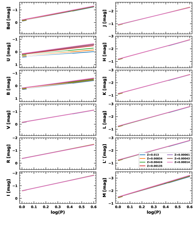
Figure 4: $PL$ relations of the BL Her models with different chemical compositions across different wavelengths for the convective parameter set A. The y-scale is same (2.5 mag) in each panel for a relative comparison. The other convection parameter sets (B, C and D) show similar $PL$ relations as a function of metallicity and wavelength.

3.3 Period-Wesenheit relations

Wesenheit indices (Madore, 1982) may be used as pseudo-magnitudes but with the added advantage that they are minimally affected by the uncertainties related to reddening corrections. A few empirical studies provide $PW$ relations instead of $PL$ relations (see example, Bhardwaj et al., 2017a). To facilitate the ease of comparison with empirical results, we provide theoretical $PW$ relations for our models. For the magnitudes ($m_{\lambda_{1}}$ and $m_{\lambda_{2}}$) in two bands ($\lambda_{1}$ and $\lambda_{2}$), the Wesenheit index may be defined as (Inno et al., 2013; Bhardwaj et al., 2016):

$$W(\lambda_{2},\lambda_{1})=m_{\lambda_{1}}-\left[\frac{A(\lambda_{1})}{E(m_{\lambda_{2}}-m_{\lambda_{1}})}\right]\times(m_{\lambda_{2}}-m_{\lambda_{1}}),$$ (7)

where $\lambda_{1}>\lambda_{2}$ and $A(\lambda_{1})/E(m_{\lambda_{2}}-m_{\lambda_{1}})$ is the total-to-selective extinction for the given filters using a particular reddening law. We adopt the reddening law from Cardelli et al. (1989) and assume $R_{V}=A(V)/(A(B)-A(V))=3.23$. For our study, we combine five optical-NIR ($VIJHK$) mean magnitudes to obtain 10 Wesenheit indices using the selective absorption ratios (Inno et al., 2013): $A_{I}/A_{V}=0.61$, $A_{J}/A_{V}=0.29$, $A_{H}/A_{V}=0.18$ and $A_{K}/A_{V}=0.12$. We derive the corresponding $PW$ relations of the mathematical form $W=a\log(P)+b$ for the BL Her models. The statistical comparison of the slopes from the theoretical NIR and optical-NIR $PW$ relations of the BL Her models using different convection parameter sets and those from previous literature is provided in Table 7. Similar to the $PL$ slopes, the BL Her models with radiative cooling (sets B and D) exhibit statistically similar $PW$ slopes across all 10 Wesenheit indices, while the models without radiative cooling (sets A and C) present larger differences for $W_{VI}$ and $W_{HK}$ indices. The theoretical $PW$ relations from the models are consistent with the empirical relations for BL Her stars in the LMC and the SMC (Matsunaga et al., 2009, 2011; Groenewegen & Jurkovic, 2017b). We note here that the differences between the theoretical $PW$ relations from the models are smaller than empirical uncertainties from the data.

Table 7: Comparison of the slopes of the NIR and optical-NIR $PW$ relations for BL Her stars of the mathematical form $W=a\log(P)+b$. $N$ is the total number of stars and the number in parentheses indicates the number of outliers. |$T$| represents the observed value of the $t$-statistic, and $p(t)$ gives the probability of acceptance of the null hypothesis (equal slopes). The bold-faced entries indicate that the null hypothesis of the equivalent $PL$ slopes can be rejected.

Band	Source	$a$	$b$	$\sigma$	$N$	Reference‡	Theoretical/ Empirical	(|$T$|, $p(t)$) w.r.t.
								Set A	Set B	Set C	Set D
$\rm{W_{VI}}$	$\rm{Z_{all}}$ (Set A)	-2.705$\pm$0.017	-1.292$\pm$0.006	0.147	3266	TW	Theoretical	…	…	…	…
$\rm{W_{VI}}$	$\rm{Z_{all}}$ (Set B)	-2.582$\pm$0.019	-1.32$\pm$0.006	0.147	2260	TW	Theoretical	(4.877,0.0)	…	…	…
$\rm{W_{VI}}$	$\rm{Z_{all}}$ (Set C)	-2.622$\pm$0.018	-1.314$\pm$0.006	0.153	2632	TW	Theoretical	(3.376,0.0)	(1.528,0.063)	…	…
$\rm{W_{VI}}$	$\rm{Z_{all}}$ (Set D)	-2.542$\pm$0.02	-1.325$\pm$0.007	0.155	2122	TW	Theoretical	(6.273,0.0)	(1.417,0.078)	(2.945,0.002)	…
$\rm{W_{VI}}$	LMC	-2.598$\pm$0.094	16.597$\pm$0.017 (@0.3)∗	0.10	55	M09	Empirical	(1.125,0.13)	(0.169,0.433)	(0.253,0.4)	(0.579,0.281)
$\rm{W_{VI}}$	LMC	-2.576$\pm$0.080	17.359$\pm$0.022	0.089	55(6)	G17	Empirical	(1.584,0.057)	(0.07,0.472)	(0.564,0.286)	(0.408,0.342)
$\rm{W_{VI}}$	@LMC†	-2.669$\pm$0.137	17.347$\pm$0.038	0.170	74(4)	G17	Empirical	(0.263,0.396)	(0.631,0.264)	(0.338,0.368)	(0.915,0.18)
$\rm{W_{VI}}$	SMC	-2.421$\pm$0.479	16.832$\pm$0.069 (@0.3)∗	0.26	17	M11	Empirical	(0.593,0.277)	(0.335,0.369)	(0.42,0.337)	(0.253,0.4)
$\rm{W_{VI}}$	SMC	-2.429$\pm$0.480	17.558$\pm$0.134	0.241	17(0)	G17	Empirical	(0.575,0.283)	(0.318,0.375)	(0.402,0.344)	(0.236,0.407)
$\rm{W_{VJ}}$	$\rm{Z_{all}}$ (Set A)	-2.584$\pm$0.018	-1.23$\pm$0.006	0.156	3266	TW	Theoretical	…	…	…	…
$\rm{W_{VJ}}$	$\rm{Z_{all}}$ (Set B)	-2.441$\pm$0.02	-1.254$\pm$0.007	0.154	2260	TW	Theoretical	(5.349,0.0)	…	…	…
$\rm{W_{VJ}}$	$\rm{Z_{all}}$ (Set C)	-2.547$\pm$0.019	-1.224$\pm$0.007	0.16	2632	TW	Theoretical	(1.422,0.078)	(3.831,0.0)	…	…
$\rm{W_{VJ}}$	$\rm{Z_{all}}$ (Set D)	-2.444$\pm$0.021	-1.238$\pm$0.007	0.161	2122	TW	Theoretical	(5.11,0.0)	(0.127,0.449)	(3.631,0.0)	…
$\rm{W_{VH}}$	$\rm{Z_{all}}$ (Set A)	-2.78$\pm$0.016	-1.396$\pm$0.005	0.142	3266	TW	Theoretical	…	…	…	…
$\rm{W_{VH}}$	$\rm{Z_{all}}$ (Set B)	-2.662$\pm$0.019	-1.424$\pm$0.006	0.143	2260	TW	Theoretical	(4.801,0.0)	…	…	…
$\rm{W_{VH}}$	$\rm{Z_{all}}$ (Set C)	-2.759$\pm$0.017	-1.411$\pm$0.006	0.144	2632	TW	Theoretical	(0.907,0.182)	(3.82,0.0)	…	…
$\rm{W_{VH}}$	$\rm{Z_{all}}$ (Set D)	-2.673$\pm$0.019	-1.424$\pm$0.007	0.148	2122	TW	Theoretical	(4.296,0.0)	(0.411,0.341)	(3.343,0.0)	…
$\rm{W_{VK}}$	$\rm{Z_{all}}$ (Set A)	-2.647$\pm$0.017	-1.251$\pm$0.006	0.15	3266	TW	Theoretical	…	…	…	…
$\rm{W_{VK}}$	$\rm{Z_{all}}$ (Set B)	-2.514$\pm$0.02	-1.276$\pm$0.006	0.15	2260	TW	Theoretical	(5.132,0.0)	…	…	…
$\rm{W_{VK}}$	$\rm{Z_{all}}$ (Set C)	-2.613$\pm$0.018	-1.253$\pm$0.006	0.153	2632	TW	Theoretical	(1.378,0.084)	(3.68,0.0)	…	…
$\rm{W_{VK}}$	$\rm{Z_{all}}$ (Set D)	-2.519$\pm$0.02	-1.266$\pm$0.007	0.156	2122	TW	Theoretical	(4.854,0.0)	(0.181,0.428)	(3.436,0.0)	…
$\rm{W_{IJ}}$	$\rm{Z_{all}}$ (Set A)	-2.541$\pm$0.018	-1.209$\pm$0.006	0.161	3266	TW	Theoretical	…	…	…	…
$\rm{W_{IJ}}$	$\rm{Z_{all}}$ (Set B)	-2.391$\pm$0.021	-1.231$\pm$0.007	0.158	2260	TW	Theoretical	(5.471,0.0)	…	…	…
$\rm{W_{IJ}}$	$\rm{Z_{all}}$ (Set C)	-2.521$\pm$0.019	-1.193$\pm$0.007	0.163	2632	TW	Theoretical	(0.758,0.224)	(4.587,0.0)	…	…
$\rm{W_{IJ}}$	$\rm{Z_{all}}$ (Set D)	-2.41$\pm$0.021	-1.208$\pm$0.007	0.165	2122	TW	Theoretical	(4.685,0.0)	(0.648,0.259)	(3.843,0.0)	…
$\rm{W_{IH}}$	$\rm{Z_{all}}$ (Set A)	-2.792$\pm$0.016	-1.412$\pm$0.005	0.142	3266	TW	Theoretical	…	…	…	…
$\rm{W_{IH}}$	$\rm{Z_{all}}$ (Set B)	-2.674$\pm$0.019	-1.44$\pm$0.006	0.143	2260	TW	Theoretical	(4.779,0.0)	…	…	…
$\rm{W_{IH}}$	$\rm{Z_{all}}$ (Set C)	-2.78$\pm$0.017	-1.426$\pm$0.006	0.143	2632	TW	Theoretical	(0.479,0.316)	(4.203,0.0)	…	…
$\rm{W_{IH}}$	$\rm{Z_{all}}$ (Set D)	-2.693$\pm$0.019	-1.439$\pm$0.007	0.147	2122	TW	Theoretical	(3.949,0.0)	(0.721,0.235)	(3.404,0.0)	…
$\rm{W_{IK}}$	$\rm{Z_{all}}$ (Set A)	-2.645$\pm$0.017	-1.251$\pm$0.006	0.151	3266	TW	Theoretical	…	…	…	…
$\rm{W_{IK}}$	$\rm{Z_{all}}$ (Set B)	-2.511$\pm$0.02	-1.275$\pm$0.006	0.15	2260	TW	Theoretical	(5.143,0.0)	…	…	…
$\rm{W_{IK}}$	$\rm{Z_{all}}$ (Set C)	-2.615$\pm$0.018	-1.251$\pm$0.006	0.153	2632	TW	Theoretical	(1.18,0.119)	(3.88,0.0)	…	…
$\rm{W_{IK}}$	$\rm{Z_{all}}$ (Set D)	-2.521$\pm$0.02	-1.264$\pm$0.007	0.156	2122	TW	Theoretical	(4.706,0.0)	(0.334,0.369)	(3.477,0.0)	…
$\rm{W_{JH}}$	$\rm{Z_{all}}$ (Set A)	-3.006$\pm$0.015	-1.587$\pm$0.005	0.137	3266	TW	Theoretical	…	…	…	…
$\rm{W_{JH}}$	$\rm{Z_{all}}$ (Set B)	-2.917$\pm$0.018	-1.621$\pm$0.006	0.139	2260	TW	Theoretical	(3.762,0.0)	…	…	…
$\rm{W_{JH}}$	$\rm{Z_{all}}$ (Set C)	-3.003$\pm$0.016	-1.627$\pm$0.006	0.136	2632	TW	Theoretical	(0.146,0.442)	(3.544,0.0)	…	…
$\rm{W_{JH}}$	$\rm{Z_{all}}$ (Set D)	-2.936$\pm$0.018	-1.639$\pm$0.006	0.142	2122	TW	Theoretical	(2.919,0.002)	(0.753,0.226)	(2.722,0.003)	…
$\rm{W_{JK}}$	$\rm{Z_{all}}$ (Set A)	-2.684$\pm$0.017	-1.268$\pm$0.006	0.148	3266	TW	Theoretical	…	…	…	…
$\rm{W_{JK}}$	$\rm{Z_{all}}$ (Set B)	-2.557$\pm$0.019	-1.294$\pm$0.006	0.147	2260	TW	Theoretical	(4.991,0.0)	…	…	…
$\rm{W_{JK}}$	$\rm{Z_{all}}$ (Set C)	-2.652$\pm$0.018	-1.275$\pm$0.006	0.15	2632	TW	Theoretical	(1.329,0.092)	(3.597,0.0)	…	…
$\rm{W_{JK}}$	$\rm{Z_{all}}$ (Set D)	-2.563$\pm$0.02	-1.287$\pm$0.007	0.153	2122	TW	Theoretical	(4.682,0.0)	(0.218,0.414)	(3.32,0.0)	…
$\rm{W_{HK}}$	$\rm{Z_{all}}$ (Set A)	-2.448$\pm$0.019	-1.035$\pm$0.006	0.168	3266	TW	Theoretical	…	…	…	…
$\rm{W_{HK}}$	$\rm{Z_{all}}$ (Set B)	-2.293$\pm$0.021	-1.054$\pm$0.007	0.163	2260	TW	Theoretical	(5.421,0.0)	…	…	…
$\rm{W_{HK}}$	$\rm{Z_{all}}$ (Set C)	-2.394$\pm$0.02	-1.016$\pm$0.007	0.172	2632	TW	Theoretical	(1.932,0.027)	(3.407,0.0)	…	…
$\rm{W_{HK}}$	$\rm{Z_{all}}$ (Set D)	-2.289$\pm$0.022	-1.029$\pm$0.008	0.171	2122	TW	Theoretical	(5.441,0.0)	(0.124,0.451)	(3.468,0.0)	…

• ^‡ TW=This work; M09=Matsunaga et al. (2009); M11=Matsunaga et al. (2011); G17=Groenewegen & Jurkovic (2017b)

• ^∗ Zero point at $\log(P)=0.3$

• ^† The stars in the LMC plus the stars in the SMC placed at the distance of the LMC by a shift of 0.432 mag

4 Period-radius relations

The mean radius obtained from averaging the radius of the BL Her model over a pulsation cycle may be used for deriving theoretical $PR$ relations for BL Her models of the mathematical form (Burki & Meylan, 1986; Marconi & Di Criscienzo, 2007):

$$\log(R/R_{\odot})=\alpha\log(P)+\beta$$ (8)

4.1 Effect of convection parameters on $PR$ relations

The $PR$ relations for BL Her models for different chemical compositions using different convective parameter sets are summarised in Table 8. The slopes and intercepts of the $PR$ relations obtained using different chemical compositions are found to be similar.

Table 8: Period-radius relations for BL Her models of the mathematical form $\log(R/R_{\odot})=\alpha\log(P)+\beta$ for different chemical compositions using different convective parameter sets.

Source	$\alpha$	$\beta$	$\sigma$	$N$
Convection set A
Z=0.00014	0.574$\pm$0.009	0.892$\pm$0.003	0.029	434
Z=0.00043	0.572$\pm$0.009	0.891$\pm$0.003	0.029	432
Z=0.00061	0.574$\pm$0.009	0.89$\pm$0.003	0.029	431
Z=0.00135	0.576$\pm$0.009	0.887$\pm$0.003	0.029	437
Z=0.00424	0.584$\pm$0.009	0.882$\pm$0.003	0.029	466
Z=0.00834	0.594$\pm$0.008	0.876$\pm$0.003	0.028	515
Z=0.01300	0.588$\pm$0.007	0.875$\pm$0.003	0.027	551
Convection set B
Z=0.00014	0.534$\pm$0.011	0.902$\pm$0.003	0.03	302
Z=0.00043	0.536$\pm$0.011	0.9$\pm$0.003	0.029	299
Z=0.00061	0.535$\pm$0.01	0.9$\pm$0.003	0.029	302
Z=0.00135	0.535$\pm$0.01	0.896$\pm$0.003	0.029	314
Z=0.00424	0.545$\pm$0.01	0.891$\pm$0.003	0.028	319
Z=0.00834	0.57$\pm$0.01	0.882$\pm$0.003	0.029	340
Z=0.01300	0.572$\pm$0.009	0.88$\pm$0.003	0.029	384
Convection set C
Z=0.00014	0.56$\pm$0.011	0.897$\pm$0.003	0.029	314
Z=0.00043	0.563$\pm$0.011	0.895$\pm$0.003	0.029	321
Z=0.00061	0.565$\pm$0.01	0.894$\pm$0.003	0.029	324
Z=0.00135	0.572$\pm$0.01	0.891$\pm$0.003	0.028	333
Z=0.00424	0.576$\pm$0.009	0.885$\pm$0.003	0.028	380
Z=0.00834	0.598$\pm$0.008	0.876$\pm$0.003	0.027	444
Z=0.01300	0.599$\pm$0.008	0.872$\pm$0.003	0.028	516
Convection set D
Z=0.00014	0.53$\pm$0.011	0.902$\pm$0.003	0.03	262
Z=0.00043	0.534$\pm$0.011	0.901$\pm$0.004	0.031	275
Z=0.00061	0.541$\pm$0.01	0.898$\pm$0.003	0.029	280
Z=0.00135	0.543$\pm$0.01	0.894$\pm$0.003	0.029	277
Z=0.00424	0.559$\pm$0.01	0.886$\pm$0.003	0.028	289
Z=0.00834	0.57$\pm$0.01	0.882$\pm$0.004	0.029	336
Z=0.01300	0.59$\pm$0.009	0.874$\pm$0.003	0.028	403

We use the statistical $t$-test (Eq. 5) to compare the slopes from the theoretical $PR$ relations across different convection parameter sets with those obtained from previous studies. The results from this test are presented in Table 9. Models with sets A and C have statistically similar $PR$ slopes while those with sets B and D show similar $PR$ slopes. We also find the slopes from the theoretical $PR$ relations of the BL Her models to be similar with those from the empirical results for the LMC and the SMC from Groenewegen & Jurkovic (2017b). Fig.5 presents a comparison of the slopes and intercepts of the $PR$ relations for the BL Her stars obtained from this work using four different convective parameter sets with those obtained from previous literature. We also use a subset of our BL Her models with the same input parameter space as that of Marconi & Di Criscienzo (2007) to compare the theoretical $PR$ relations; the results are displayed in Fig.5.

Table 9: Comparison of the slopes of the $PR$ relations for BL Her stars of the mathematical form $\log(R/R_{\odot})=\alpha\log(P)+\beta$. $N$ is the total number of stars and the number in parentheses indicates the number of outliers. |$T$| represents the observed value of the $t$-statistic, and $p(t)$ gives the probability of acceptance of the null hypothesis (equal slopes). The bold-faced entries indicate that the null hypothesis of the equivalent $PR$ slopes can be rejected.

Source	$\alpha$	$\beta$	$\sigma$	$N$	Reference‡	Theoretical/ Empirical	(|$T$|, $p(t)$) w.r.t.
							Set A	Set B	Set C	Set D
$\rm{Z_{all}}$ (Set A)	0.576$\pm$0.003	0.886$\pm$0.001	0.029	3266	TW	Theoretical	…	…	…	…
$\rm{Z_{all}}$ (Set B)	0.545$\pm$0.004	0.893$\pm$0.001	0.029	2260	TW	Theoretical	(6.278,0.0)	…	…	…
$\rm{Z_{all}}$ (Set C)	0.574$\pm$0.003	0.888$\pm$0.001	0.029	2632	TW	Theoretical	(0.588,0.278)	(5.595,0.0)	…	…
$\rm{Z_{all}}$ (Set D)	0.55$\pm$0.004	0.891$\pm$0.001	0.029	2122	TW	Theoretical	(5.17,0.0)	(1.046,0.148)	(4.509,0.0)	…
LMC	0.564$\pm$0.049	0.830$\pm$0.013	0.047	57(4)	G17	Empirical	(0.253,0.4)	(0.39,0.348)	(0.197,0.422)	(0.275,0.392)
SMC	0.574$\pm$0.117	0.852$\pm$0.028	0.056	17(0)	G17	Empirical	(0.021,0.492)	(0.249,0.402)	(0.003,0.499)	(0.201,0.42)
MCs	0.551$\pm$0.052	0.847$\pm$0.013	0.058	76(2)	G17	Empirical	(0.488,0.313)	(0.119,0.453)	(0.435,0.332)	(0.01,0.496)
Galactic T2Cs	0.54	0.87	-	-	B86∗	Empirical	-	-	-	-
$\rm{Z_{all}}$	0.529$\pm$0.006	0.87$\pm$0.01	-	-	M07∗	Theoretical	-	-	-	-

• ^‡ TW=This work; G17=Groenewegen & Jurkovic (2017b); B86=Burki & Meylan (1986); M07=Marconi & Di Criscienzo (2007)

• ^∗ Data insufficient to determine the value of the $t$-statistic and the associated probability value.

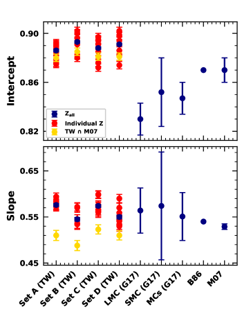
Figure 5: A comparison of the slopes and intercepts of the $PR$ relations for the BL Her stars obtained from this work (TW) using four different convective parameter sets with those obtained from previous literature. The red dots refer to the slopes and intercepts of the $PR$ relations obtained for the different chemical compositions individually, while the blue dots refer to the results obtained from considering the entire range of chemical compositions ($Z=0.00014-Z=0.013$) together. The yellow dots represent the subset of the model grid of this work with the same parameter space as that of Marconi & Di Criscienzo (2007). G17, B86 and M07 refer to Groenewegen & Jurkovic (2017b), Burki & Meylan (1986) and Marconi & Di Criscienzo (2007), respectively.

4.2 Effect of metallicity on $PR$ relations

To test for the effect of metallicity on the $PR$ relations, we derive $PRZ$ relations of the form:

$$\log(R/R_{\odot})=\alpha+\beta\log(P)+\gamma\mathrm{[Fe/H]}$$ (9)

for the four different convection parameter sets. We find the following relations for set A:

$$\log(R/R_{\odot})={} (0.879\pm 0.001)+(0.581\pm 0.003)\log(P)$$ (10)

$$-(0.006\pm 0.001)\mathrm{[Fe/H]}\>(N=3266;\sigma=0.029),$$

for set B:

$$\log(R/R_{\odot})={} (0.888\pm 0.002)+(0.548\pm 0.004)\log(P)$$ (11)

$$-(0.006\pm 0.001)\mathrm{[Fe/H]}\>(N=2260;\sigma=0.029),$$

for set C:

$$\log(R/R_{\odot})= {}(0.881\pm 0.001)+(0.579\pm 0.003)\log(P)$$ (12)

$$-(0.006\pm 0.001)\mathrm{[Fe/H]}\>(N=2632;\sigma=0.028),$$

and for set D:

$$\log(R/R_{\odot})= {}(0.886\pm 0.002)+(0.554\pm 0.004)\log(P)$$ (13)

$$-(0.006\pm 0.001)\mathrm{[Fe/H]}\>(N=2122;\sigma=0.029)$$

From Eqs. 10-13, we find the coefficients of the metallicity term to be very small for all four convection parameter sets and thus, we may conclude that there is weak dependence of $PR$ relations on metallicity. This is in agreement with previous empirical results from Burki & Meylan (1986), Balog et al. (1997) and Groenewegen & Jurkovic (2017b). We also find that the dependency of $PR$ relations on metallicity is identical for all four sets of convection parameters.

5 Comparison with RR Lyrae models

RR Lyrae and BL Her stars are pulsating variables that belong to old stellar populations of similar chemical compositions. Both classes are population II pulsating stars and offer an important alternative tool to classical Cepheids to calibrate the cosmic distance scale and evaluate the Hubble constant. Majaess (2010) presented preliminary evidence of a common $PL$ relation for RR Lyrae and T2Cs. Bhardwaj et al. (2017a) showed that the $PL$ relation of T2Cs in $K$-band when extended to periods less than 1 day follow the same $PL$ relation as RR Lyrae stars. They also demonstrated that distances to the GGCs based on T2Cs are consistent with those based on horizontal branch (HB) stars. In the most recent study, Braga et al. (2020) derived $PL$ relations of RR Lyrae and T2Cs in $\omega$ Cen and found empirical evidence that RRab and T2Cs indeed obey the same $JHK_{S}$ $PL$ relations.

To test this equivalence between RR Lyrae and T2Cs, we compare the theoretical relations from our BL Her models with the most recent grid of RR Lyrae models from Marconi et al. (2015). Table 10 presents the comparison of the $PL$ slopes in $RIJHK_{S}$ bands for RR Lyrae models from Marconi et al. (2015) with those obtained from the BL Her models of our work. The RR Lyrae models exhibit statistically similar $PL$ slopes in the bands, $RIJK_{S}$ with those from the BL Her models computed using sets A and C. A possible explanation for the slopes not being statistically similar with BL Her models computed using sets B and D is that the RR Lyrae models from Marconi et al. (2015) are computed without radiative cooling. Our grid of BL Her models therefore supports the claim by Braga et al. (2020) that the equivalence of the $PL$ relations of RR Lyrae and T2Cs gives us the opportunity of adopting RRLs+T2Cs together as an alternative to classical Cepheids for the extragalactic distance scale calibration.

From Table 10, we also find that the $PR$ slope of the RR Lyrae models from Marconi et al. (2015) is statistically similar with those obtained from the BL Her models in all four sets of convection parameters. This is in support of the result obtained by Marconi et al. (2015) where they found similar $PR$ slopes for RR Lyrae models with theoretical and empirical BL Her $PR$ slopes from Marconi & Di Criscienzo (2007) and Burki & Meylan (1986), respectively. This therefore suggests tight correlation of evolutionary and pulsational properties of the two classes of evolved low-mass radial variables. A detailed comparison of RR Lyrae and BL Her pulsation properties could be useful to probe an evolutionary scenario where BL Hers are HB stars that have evolved off the HB and are moving up the Asymptotic Giant Branch (AGB). BL Her stars may then be considered as the evolved component of RR Lyrae stars Marconi et al. (2011); Marconi et al. (2015). Marconi et al. (2015) cautions that this similarity between BL Her and RR Lyrae may not be extended over the entire metallicity range. We note here that Marconi et al. (2015) uses the convection formulation outlined in Stellingwerf (1982a, b) while mesa-rsp uses Kuhfuss (1986) turbulent convection theory; it is therefore interesting to obtain similar $PL$ and $PR$ results for RR Lyrae and BL Her models using different theories of convection.

Table 10: Comparison of the slopes of the period-luminosity and period-radius relations of the mathematical forms $M_{\lambda}=a\log(P)+b$ and $\log(R/R_{\odot})=\alpha\log(P)+\beta$, respectively for RR Lyrae models from Marconi et al. (2015). $N$ is the total number of models. |$T$| represents the observed value of the $t$-statistic, and $p(t)$ gives the probability of acceptance of the null hypothesis (equal slopes). The bold-faced entries indicate that the null hypothesis of the equivalent $PL$ slopes can be rejected.

Band	Source	Slope	Intercept	$\sigma$	$N$	Reference‡	Theoretical/ Empirical	(|$T$|, $p(t)$) w.r.t. This work
								Set A	Set B	Set C	Set D
Period-luminosity relation
R	$\rm{Z_{all}}$	-1.756$\pm$0.077	-0.114$\pm$0.014	0.196	226	M15	Theoretical	(1.19,0.117)	(1.485,0.069)	(0.208,0.418)	(1.882,0.03)
I	$\rm{Z_{all}}$	-1.973$\pm$0.068	-0.415$\pm$0.013	0.175	226	M15	Theoretical	(0.966,0.167)	(1.709,0.044)	(0.561,0.287)	(2.217,0.013)
J	$\rm{Z_{all}}$	-2.245$\pm$0.06	-0.778$\pm$0.011	0.155	226	M15	Theoretical	(0.902,0.184)	(1.769,0.039)	(0.098,0.461)	(1.898,0.029)
H	$\rm{Z_{all}}$	-2.206$\pm$0.118	-1.043$\pm$0.022	0.302	226	M15	Theoretical	(3.056,0.001)	(1.867,0.031)	(2.708,0.003)	(1.889,0.03)
K	$\rm{Z_{all}}$	-2.514$\pm$0.057	-1.11$\pm$0.011	0.147	226	M15	Theoretical	(0.24,0.405)	(2.149,0.016)	(0.507,0.306)	(2.149,0.016)
Period-radius relation
$-$	$\rm{Z_{all}}$	0.557$\pm$0.011	0.871$\pm$0.002	0.029	226	M15	Theoretical	(1.622,0.052)	(1.015,0.155)	(1.45,0.074)	(0.596,0.276)

• ^‡ M15=Marconi et al. (2015)

• The $PL$ and $PR$ relations for the RR Lyrae models have been obtained using Table 3 of Marconi et al. (2015). The $PL$ and $PR$ relations for the BL Her models computed in this work using the four sets of convection parameters are available in Table 5 and Table 9, respectively.

6 Summary and Conclusion

We computed a very fine grid of BL Her models using the most recent, state-of-the-art stellar pulsation code, the mesa-rsp (Paxton et al., 2019). The grid encompasses a wide range of metallicity, mass, luminosity and effective temperature with four different sets of convection parameters, A, B, C and D as outlined in Paxton et al. (2019) and Table 1. The metallicity varies from [Fe/H]=-2.0 dex ($Z$=0.00014) to [Fe/H]=0.0 dex ($Z$=0.013). The stellar masses vary from 0.5M_⊙ to 0.8M_⊙, while the stellar luminosity varies from 50L_⊙ to 300L_⊙, typical for BL Her stars. Effective temperature is in steps of 50 K inside the instability strip. Non-linear models were computed for 4000 pulsation cycles for periods typical for BL Her stars, i.e. $1\leq\mathrm{P(days)}\leq 4$. The non-linear models analysed in this study fulfil the condition of full-amplitude stable pulsations, i.e., amplitude of radius variation $\Delta R$, period $P$ and fractional growth rate $\Gamma$ do not vary by more than 0.01 over the last $\sim$100-cycles of the total 4000-cycle integrations. The total number of BL Her models accepted are 3266 in set A, 2260 in set B, 2632 in set C and 2122 in set D. We have theoretical lightcurves in multiple wavelengths, $UBVRIJHKLL^{\prime}M$ from the computed non-linear models.

We obtain theoretical multi-wavelength $PL$, $PW$ and $PR$ relations for these models using the four different sets of convection parameters. We test for the effect of metallicity and convection parameters on the $PL$ and $PR$ relations. We summarise the important results below:

1. Models computed with sets B and D show statistically similar slopes for $PL$, $PW$ and $PR$ relations while those with sets A and C exhibit similar slopes for most cases. Sets B and D are the models computed with radiative cooling; sets A and C are computed without radiative cooling.

2. Most empirical relations match well with the theoretical $PL$, $PW$ and $PR$ relations derived using our BL Her models and over all the four sets of convection parameters.

3. An exception to this are the $PL$ relations for BL Her stars in the LMC where $PL$ slopes of the models with sets B and D seem to match better with empirical relations in the $HK_{S}$ bands.

4. We find that the $PL$ slopes from the BL Her models become steeper with increasing wavelengths. The dispersion in the theoretical $PL$ relations for BL Hers decreases significantly moving from optical to infrared wavelengths and becomes statistically similar for wavelengths longer than $H$-band. We also observe that the models computed using set B have the smallest dispersion in their $PL$ relations in all the bands.

5. For each set of convection parameters, the effect of metallicity is significant in $U$ and $B$-bands, and appreciable for bolometric $PL$ relations. It is much weaker in redder bands, consistent with empirical data and previous studies (Matsunaga et al., 2006; Groenewegen & Jurkovic, 2017b).

6. There is a weak dependence of the $PR$ relations on metallicity with identical coefficient (0.006 $\pm$ 0.001) for all 4 sets of convection parameters. The inclusion of the metallicity term does not lead to a significant decrease in dispersion for the relations. This is consistent with the empirical evidence from Burki & Meylan (1986), Balog et al. (1997) and Groenewegen & Jurkovic (2017b).

7. The RR Lyrae models from Marconi et al. (2015) exhibit statistically similar $PL$ relations in the $RIJK_{S}$ bands with those obtained from BL Her models computed using sets A and C while the $PR$ slopes from the RR Lyrae models are statistically similar with the relations from the BL Her models using all four sets of convection parameters.

However, it is important to note here that both the $PL$ and the $PR$ relations derived in this study are at mean light, which averages out the effect of the pulsation cycle. We also note that the comparison among the models computed using different sets of convection parameters has higher precision than when comparing with empirical $PL$ and $PW$ relations. It would seem that observations are not yet sufficiently precise to distinguish fully among the models, although there is a preference for the models that include radiative cooling. It would be interesting to study the effect of different convective parameter sets on the light curve structures of the BL Her models during the pulsation cycle, which we plan to investigate in a future project. The large number of models computed in this study ushers in the era of large number statistics in the analysis of theoretical models.

Data Availability

The data underlying this article are available in the article and in its online supplementary material.

Appendix A $PL$ relations using different model atmospheres

mesa provides two sets of pre-processed tables of bolometric corrections (Paxton et al., 2018). The results discussed in this work are using the pre-processed table ($\rm{BC_{1}}$) from Lejeune et al. (1998). To test the impact of the adopted model atmospheres used to transform bolometric light curves to observational bands, we use another pre-processed table ($\rm{BC_{2}}$) which provides a set of blackbody bolometric corrections for the bands $UBVR_{c}I_{c}$ over the range $100\leq T_{\rm{eff}}\rm{(K)}\leq 50,000$, in steps of 100 K. For the exact same set of models, we compare the slopes of the $PL$ relations in the $V$ and $I$ bands of the mathematical form $\rm{\log_{10}(L_{V/I}/L_{\odot})}=a\log(P)+b$ using the two different sets of bolometric corrections, $\rm{BC_{1}}$ and $\rm{BC_{2}}$. We find the $PL_{V}$ slopes to be $0.657\pm 0.013$ and $0.68\pm 0.012$ for 3266 BL Her models in set A, $0.552\pm 0.014$ and $0.584\pm 0.013$ for 2260 models in set B, $0.6\pm 0.014$ and $0.616\pm 0.013$ for 2633 models in set C and $0.535\pm 0.014$ and $0.559\pm 0.014$ for 2122 models in set D using the two different bolometric correction sets $\rm{BC_{1}}$ and $\rm{BC_{2}}$, respectively. The slopes of the $PL$ relations in the $V$ band differ by less than 6% when a different model atmosphere incorporated in mesa is adopted. For the $I$-band, the $PL$ slopes are $0.825\pm 0.01$ and $0.809\pm 0.01$ in set A, $0.741\pm 0.011$ and $0.728\pm 0.011$ in set B, $0.777\pm 0.011$ and $0.763\pm 0.011$ in set C and $0.724\pm 0.011$ and $0.712\pm 0.011$ in set D using the different bolometric correction sets $\rm{BC_{1}}$ and $\rm{BC_{2}}$, respectively. The slopes of the $PL$ relations in the $I$ band therefore differ by less than 2% when a different model atmosphere is adopted. We find significant variation in $PL$ slopes in $U$ and $B$-band when the two different bolometric sets are adopted. The effect of different model atmospheres on transformations of bolometric light curves to observational bands reduces as we move to longer wavelengths. We note here that the mean luminosity used for these relations have been obtained from averaging the luminosity of the BL Her model over a pulsation cycle, unlike the mean magnitudes obtained from Fourier fitting as discussed in Section 3.

The reason for adopting the bolometric correction set $\rm{BC_{1}}$ in our present work is that it provides bolometric corrections for the Johnson-Cousins-Class bands $UBVRIJHKLL^{\prime}M$ while $\rm{BC_{2}}$ only provides bolometric corrections for $UBVR_{c}I_{c}$. $\rm{BC_{1}}$ defines the bolometric correction as a function of the stellar photosphere; $T_{\rm{eff}}\rm{(K)}$, $\log(g)\rm{(cms^{-2})}$, and the metallicity $[M/H]$. Since $\rm{BC_{2}}$ involves blackbody corrections, there is no $g$ or $[M/H]$ dependence. While a more detailed and quantitative comparison using other model atmospheres is important, it is beyond the scope of this paper and we do not anticipate much difference since we are primarily concerned with $PL$ relations at mean light. Using the two different bolometric correction sets provided by mesa also suggests that the change in $PL$ slopes due to different adopted model transformations is minimal at wavelengths longer than $V$-band. In addition, Paxton et al. (2019) demonstrates that the mesa-rsp code produces stable, multi-wavelength light curve models with reasonable comparison with observations for a wide class of radially pulsating stars. Further, Das et al. (2020) obtained theoretical period-colour relations for a broad spectrum of variable stars, including BL Hers which were in broad agreement with observations.

Appendix B $PLZ$ relations in the low and high-metallicity regimes

To investigate the dependence of $PL$ relations on metallicity, we separated models in low-metallicity ($Z=0.00014,0.00043,0.00061,0.00135$) and high-metallicity ($Z=0.00424,0.00834,0.01300$) regime. The results of $PLZ$ relations for the models in the low and high-metallicity regimes using different convection sets are listed in Tables 11 and 12, respectively and discussed in Section 3.2.

Table 11: $PLZ$ relations of the mathematical form $M_{\lambda}=a+b\log(P)+c\mathrm{[Fe/H]}$ for BL Her models in the low-metallicity regime ($Z=0.00014,0.00043,0.00061,0.00135$) for different wavelengths using different convective parameter sets.

Band	$a$	$b$	$c$	$\sigma$	$N$
Convection set A
U	0.305 $\pm$ 0.036	-1.217 $\pm$ 0.052	0.105 $\pm$ 0.022	0.324	1734
B	0.207 $\pm$ 0.038	-1.273 $\pm$ 0.055	0.027 $\pm$ 0.023	0.34	1734
V	-0.163 $\pm$ 0.032	-1.605 $\pm$ 0.046	-0.01 $\pm$ 0.019	0.285	1734
R	-0.39 $\pm$ 0.028	-1.827 $\pm$ 0.04	-0.015 $\pm$ 0.017	0.25	1734
I	-0.611 $\pm$ 0.024	-2.024 $\pm$ 0.035	-0.009 $\pm$ 0.015	0.22	1734
J	-0.93 $\pm$ 0.021	-2.268 $\pm$ 0.03	-0.003 $\pm$ 0.013	0.189	1734
H	-1.179 $\pm$ 0.018	-2.543 $\pm$ 0.026	0.005 $\pm$ 0.011	0.159	1734
K	-1.134 $\pm$ 0.018	-2.499 $\pm$ 0.026	0.005 $\pm$ 0.011	0.163	1734
L	-1.239 $\pm$ 0.017	-2.574 $\pm$ 0.025	0.006 $\pm$ 0.01	0.157	1734
L’	-1.242 $\pm$ 0.017	-2.576 $\pm$ 0.025	0.007 $\pm$ 0.01	0.157	1734
M	-1.482 $\pm$ 0.015	-2.842 $\pm$ 0.022	0.018 $\pm$ 0.009	0.14	1734
Bolometric	-0.176 $\pm$ 0.028	-1.806 $\pm$ 0.041	0.022 $\pm$ 0.017	0.253	1734
Convection set B
U	0.344 $\pm$ 0.035	-0.958 $\pm$ 0.049	0.117 $\pm$ 0.022	0.271	1217
B	0.245 $\pm$ 0.037	-1.006 $\pm$ 0.051	0.035 $\pm$ 0.023	0.286	1217
V	-0.14 $\pm$ 0.032	-1.372 $\pm$ 0.044	-0.005 $\pm$ 0.02	0.246	1217
R	-0.375 $\pm$ 0.028	-1.616 $\pm$ 0.039	-0.01 $\pm$ 0.017	0.22	1217
I	-0.605 $\pm$ 0.026	-1.833 $\pm$ 0.035	-0.005 $\pm$ 0.016	0.198	1217
J	-0.935 $\pm$ 0.023	-2.09 $\pm$ 0.031	0.002 $\pm$ 0.014	0.174	1217
H	-1.195 $\pm$ 0.02	-2.386 $\pm$ 0.027	0.009 $\pm$ 0.012	0.153	1217
K	-1.148 $\pm$ 0.02	-2.338 $\pm$ 0.028	0.009 $\pm$ 0.012	0.156	1217
L	-1.255 $\pm$ 0.02	-2.419 $\pm$ 0.027	0.01 $\pm$ 0.012	0.152	1217
L’	-1.258 $\pm$ 0.02	-2.421 $\pm$ 0.027	0.011 $\pm$ 0.012	0.152	1217
M	-1.508 $\pm$ 0.018	-2.709 $\pm$ 0.025	0.022 $\pm$ 0.011	0.14	1217
Bolometric	-0.162 $\pm$ 0.029	-1.58 $\pm$ 0.04	0.027 $\pm$ 0.018	0.222	1217
Convection set C
U	0.414 $\pm$ 0.041	-0.792 $\pm$ 0.056	0.129 $\pm$ 0.025	0.318	1292
B	0.327 $\pm$ 0.041	-0.935 $\pm$ 0.057	0.039 $\pm$ 0.025	0.323	1292
V	-0.077 $\pm$ 0.035	-1.362 $\pm$ 0.048	-0.008 $\pm$ 0.021	0.273	1292
R	-0.328 $\pm$ 0.031	-1.618 $\pm$ 0.043	-0.014 $\pm$ 0.019	0.242	1292
I	-0.57 $\pm$ 0.028	-1.843 $\pm$ 0.038	-0.009 $\pm$ 0.017	0.217	1292
J	-0.91 $\pm$ 0.024	-2.142 $\pm$ 0.033	-0.005 $\pm$ 0.015	0.188	1292
H	-1.184 $\pm$ 0.02	-2.472 $\pm$ 0.028	0.002 $\pm$ 0.012	0.16	1292
K	-1.136 $\pm$ 0.021	-2.415 $\pm$ 0.029	0.002 $\pm$ 0.013	0.164	1292
L	-1.246 $\pm$ 0.02	-2.506 $\pm$ 0.028	0.003 $\pm$ 0.012	0.158	1292
L’	-1.248 $\pm$ 0.02	-2.509 $\pm$ 0.028	0.004 $\pm$ 0.012	0.157	1292
M	-1.507 $\pm$ 0.018	-2.823 $\pm$ 0.025	0.017 $\pm$ 0.011	0.14	1292
Bolometric	-0.111 $\pm$ 0.031	-1.606 $\pm$ 0.043	0.024 $\pm$ 0.019	0.245	1292
Convection set D
U	0.429 $\pm$ 0.038	-0.762 $\pm$ 0.05	0.127 $\pm$ 0.024	0.28	1094
B	0.334 $\pm$ 0.04	-0.87 $\pm$ 0.052	0.033 $\pm$ 0.025	0.29	1094
V	-0.075 $\pm$ 0.034	-1.28 $\pm$ 0.045	-0.01 $\pm$ 0.021	0.251	1094
R	-0.327 $\pm$ 0.031	-1.536 $\pm$ 0.04	-0.015 $\pm$ 0.019	0.226	1094
I	-0.569 $\pm$ 0.028	-1.76 $\pm$ 0.037	-0.008 $\pm$ 0.017	0.205	1094
J	-0.912 $\pm$ 0.025	-2.047 $\pm$ 0.033	-0.001 $\pm$ 0.016	0.183	1094
H	-1.188 $\pm$ 0.022	-2.369 $\pm$ 0.029	0.008 $\pm$ 0.014	0.161	1094
K	-1.139 $\pm$ 0.023	-2.314 $\pm$ 0.029	0.008 $\pm$ 0.014	0.164	1094
L	-1.25 $\pm$ 0.022	-2.402 $\pm$ 0.029	0.01 $\pm$ 0.014	0.16	1094
L’	-1.252 $\pm$ 0.022	-2.405 $\pm$ 0.029	0.011 $\pm$ 0.014	0.16	1094
M	-1.513 $\pm$ 0.02	-2.715 $\pm$ 0.026	0.026 $\pm$ 0.012	0.146	1094
Bolometric	-0.109 $\pm$ 0.031	-1.511 $\pm$ 0.041	0.023 $\pm$ 0.019	0.227	1094

Table 12: $PLZ$ relations of the mathematical form $M_{\lambda}=a+b\log(P)+c\mathrm{[Fe/H]}$ for BL Her models in the high-metallicity regime ($Z=0.00424,0.00834,0.01300$) for different wavelengths using different convective parameter sets.

Band	$a$	$b$	$c$	$\sigma$	$N$
Convection set A
U	0.432 $\pm$ 0.026	-0.816 $\pm$ 0.062	0.442 $\pm$ 0.048	0.382	1532
B	0.288 $\pm$ 0.024	-1.187 $\pm$ 0.057	0.173 $\pm$ 0.045	0.353	1532
V	-0.118 $\pm$ 0.019	-1.642 $\pm$ 0.046	0.043 $\pm$ 0.036	0.282	1532
R	-0.358 $\pm$ 0.017	-1.873 $\pm$ 0.04	0.015 $\pm$ 0.031	0.245	1532
I	-0.579 $\pm$ 0.015	-2.066 $\pm$ 0.035	0.027 $\pm$ 0.027	0.217	1532
J	-0.89 $\pm$ 0.012	-2.347 $\pm$ 0.03	0.025 $\pm$ 0.023	0.182	1532
H	-1.135 $\pm$ 0.01	-2.621 $\pm$ 0.025	0.039 $\pm$ 0.019	0.153	1532
K	-1.086 $\pm$ 0.011	-2.583 $\pm$ 0.025	0.041 $\pm$ 0.02	0.157	1532
L	-1.192 $\pm$ 0.01	-2.652 $\pm$ 0.025	0.044 $\pm$ 0.019	0.152	1532
L’	-1.193 $\pm$ 0.01	-2.652 $\pm$ 0.025	0.048 $\pm$ 0.019	0.152	1532
M	-1.427 $\pm$ 0.01	-2.833 $\pm$ 0.023	0.103 $\pm$ 0.018	0.14	1532
Bolometric	-0.108 $\pm$ 0.017	-1.864 $\pm$ 0.04	0.092 $\pm$ 0.031	0.248	1532
Convection set B
U	0.411 $\pm$ 0.027	-0.428 $\pm$ 0.069	0.385 $\pm$ 0.053	0.35	1043
B	0.269 $\pm$ 0.025	-0.847 $\pm$ 0.064	0.1 $\pm$ 0.05	0.328	1043
V	-0.141 $\pm$ 0.02	-1.372 $\pm$ 0.052	-0.02 $\pm$ 0.04	0.267	1043
R	-0.383 $\pm$ 0.018	-1.638 $\pm$ 0.046	-0.041 $\pm$ 0.036	0.235	1043
I	-0.606 $\pm$ 0.016	-1.856 $\pm$ 0.041	-0.021 $\pm$ 0.032	0.21	1043
J	-0.921 $\pm$ 0.014	-2.175 $\pm$ 0.035	-0.02 $\pm$ 0.027	0.18	1043
H	-1.168 $\pm$ 0.012	-2.488 $\pm$ 0.03	0.002 $\pm$ 0.024	0.155	1043
K	-1.119 $\pm$ 0.012	-2.445 $\pm$ 0.031	0.002 $\pm$ 0.024	0.158	1043
L	-1.225 $\pm$ 0.012	-2.522 $\pm$ 0.03	0.008 $\pm$ 0.023	0.153	1043
L’	-1.227 $\pm$ 0.012	-2.522 $\pm$ 0.03	0.011 $\pm$ 0.023	0.154	1043
M	-1.462 $\pm$ 0.011	-2.727 $\pm$ 0.028	0.076 $\pm$ 0.022	0.143	1043
Bolometric	-0.134 $\pm$ 0.018	-1.622 $\pm$ 0.046	0.032 $\pm$ 0.036	0.237	1043
Convection set C
U	0.605 $\pm$ 0.031	-0.553 $\pm$ 0.074	0.46 $\pm$ 0.06	0.438	1340
B	0.465 $\pm$ 0.027	-1.097 $\pm$ 0.064	0.143 $\pm$ 0.052	0.38	1340
V	0.012 $\pm$ 0.021	-1.602 $\pm$ 0.05	0.009 $\pm$ 0.041	0.3	1340
R	-0.261 $\pm$ 0.019	-1.828 $\pm$ 0.044	-0.016 $\pm$ 0.036	0.263	1340
I	-0.509 $\pm$ 0.017	-2.008 $\pm$ 0.039	0.003 $\pm$ 0.032	0.234	1340
J	-0.849 $\pm$ 0.014	-2.324 $\pm$ 0.032	-0.003 $\pm$ 0.026	0.192	1340
H	-1.127 $\pm$ 0.011	-2.601 $\pm$ 0.027	0.02 $\pm$ 0.022	0.16	1340
K	-1.074 $\pm$ 0.012	-2.563 $\pm$ 0.027	0.019 $\pm$ 0.022	0.163	1340
L	-1.186 $\pm$ 0.011	-2.634 $\pm$ 0.026	0.024 $\pm$ 0.021	0.158	1340
L’	-1.187 $\pm$ 0.011	-2.635 $\pm$ 0.027	0.028 $\pm$ 0.021	0.158	1340
M	-1.447 $\pm$ 0.01	-2.796 $\pm$ 0.024	0.101 $\pm$ 0.02	0.145	1340
Bolometric	-0.004 $\pm$ 0.019	-1.843 $\pm$ 0.044	0.06 $\pm$ 0.036	0.262	1340
Convection set D
U	0.545 $\pm$ 0.034	-0.275 $\pm$ 0.083	0.399 $\pm$ 0.066	0.428	1028
B	0.412 $\pm$ 0.03	-0.844 $\pm$ 0.073	0.078 $\pm$ 0.058	0.375	1028
V	-0.028 $\pm$ 0.023	-1.403 $\pm$ 0.058	-0.043 $\pm$ 0.046	0.297	1028
R	-0.294 $\pm$ 0.02	-1.659 $\pm$ 0.05	-0.06 $\pm$ 0.04	0.26	1028
I	-0.536 $\pm$ 0.018	-1.862 $\pm$ 0.045	-0.034 $\pm$ 0.036	0.231	1028
J	-0.87 $\pm$ 0.015	-2.208 $\pm$ 0.037	-0.034 $\pm$ 0.03	0.191	1028
H	-1.14 $\pm$ 0.013	-2.519 $\pm$ 0.031	-0.003 $\pm$ 0.025	0.16	1028
K	-1.089 $\pm$ 0.013	-2.477 $\pm$ 0.032	-0.005 $\pm$ 0.025	0.164	1028
L	-1.199 $\pm$ 0.012	-2.554 $\pm$ 0.031	0.003 $\pm$ 0.025	0.158	1028
L’	-1.2 $\pm$ 0.012	-2.555 $\pm$ 0.031	0.006 $\pm$ 0.025	0.158	1028
M	-1.454 $\pm$ 0.012	-2.739 $\pm$ 0.028	0.088 $\pm$ 0.023	0.147	1028
Bolometric	-0.038 $\pm$ 0.02	-1.667 $\pm$ 0.05	0.011 $\pm$ 0.04	0.26	1028

References

- Allard & Hauschildt (1995) Allard F., Hauschildt P. H., 1995, ApJ, 445, 433
- Asplund et al. (2009) Asplund M., Grevesse N., Sauval A. J., Scott P., 2009, ARA&A, 47, 481
- Balog et al. (1997) Balog Z., Vinko J., Kaszas G., 1997, AJ, 113, 1833
- Beaton et al. (2018) Beaton R. L., et al., 2018, SSRv, 214, 113
- Bessell et al. (1989) Bessell M. S., Brett J. M., Scholz M., Wood P. R., 1989, A&AS, 77, 1
- Bessell et al. (1991) Bessell M. S., Brett J. M., Scholz M., Wood P. R., 1991, A&AS, 89, 335
- Bhardwaj (2020) Bhardwaj A., 2020, Journal of Astrophysics and Astronomy, 41, 23
- Bhardwaj et al. (2015) Bhardwaj A., Kanbur S. M., Singh H. P., Macri L. M., Ngeow C.-C., 2015, MNRAS, 447, 3342
- Bhardwaj et al. (2016) Bhardwaj A., Kanbur S. M., Macri L. M., Singh H. P., Ngeow C.-C., Wagner-Kaiser R., Sarajedini A., 2016, AJ, 151, 88
- Bhardwaj et al. (2017a) Bhardwaj A., Macri L. M., Rejkuba M., Kanbur S. M., Ngeow C.-C., Singh H. P., 2017a, AJ, 153, 154
- Bhardwaj et al. (2017b) Bhardwaj A., et al., 2017b, A&A, 605, A100
- Bhardwaj et al. (2020) Bhardwaj A., Rejkuba M., de Grijs R., Herczeg G. J., Singh H. P., Kanbur S., Ngeow C.-C., 2020, AJ, 160, 220
- Bono et al. (1995) Bono G., Castellani V., Stellingwerf R. F., 1995, ApJL, 445, L145
- Bono et al. (1997a) Bono G., Caputo F., Santolamazza P., 1997a, A&A, 317, 171
- Bono et al. (1997b) Bono G., Caputo F., Cassisi S., Castellani V., Marconi M., 1997b, ApJ, 489, 822
- Bono et al. (2003) Bono G., Caputo F., Castellani V., Marconi M., Storm J., Degl’Innocenti S., 2003, MNRAS, 344, 1097
- Braga et al. (2018) Braga V. F., Bhardwaj A., Contreras Ramos R., Minniti D., Bono G., de Grijs R., Minniti J. H., Rejkuba M., 2018, A&A, 619, A51
- Braga et al. (2020) Braga V. F., et al., 2020, arXiv e-prints, p. arXiv:2010.06368
- Buchler & Moskalik (1992) Buchler J. R., Moskalik P., 1992, ApJ, 391, 736
- Burki & Meylan (1986) Burki G., Meylan G., 1986, A&A, 159, 261
- Cardelli et al. (1989) Cardelli J. A., Clayton G. C., Mathis J. S., 1989, ApJ, 345, 245
- Catelan et al. (2004) Catelan M., Pritzl B. J., Smith H. A., 2004, ApJS, 154, 633
- Ciechanowska et al. (2010) Ciechanowska A., Pietrzyński G., Szewczyk O., Gieren W., Soszyński I., 2010, AcA, 60, 233
- Cioni et al. (2011) Cioni M. R. L., et al., 2011, A&A, 527, A116
- Clement et al. (2001) Clement C. M., et al., 2001, AJ, 122, 2587
- Clementini et al. (2016) Clementini G., et al., 2016, A&A, 595, A133
- Das et al. (2018) Das S., Bhardwaj A., Kanbur S. M., Singh H. P., Marconi M., 2018, MNRAS, 481, 2000
- Das et al. (2020) Das S., et al., 2020, MNRAS, 493, 29
- Deb & Singh (2009) Deb S., Singh H. P., 2009, A&A, 507, 1729
- Di Criscienzo et al. (2007) Di Criscienzo M., Caputo F., Marconi M., Cassisi S., 2007, A&A, 471, 893
- Ferguson et al. (2005) Ferguson J. W., Alexander D. R., Allard F., Barman T., Bodnarik J. G., Hauschildt P. H., Heffner-Wong A., Tamanai A., 2005, ApJ, 623, 585
- Fluks et al. (1994) Fluks M. A., Plez B., The P. S., de Winter D., Westerlund B. E., Steenman H. C., 1994, A&AS, 105, 311
- Gray (2005) Gray D. F., 2005, The Observation and Analysis of Stellar Photospheres
- Groenewegen & Jurkovic (2017a) Groenewegen M. A. T., Jurkovic M. I., 2017a, A&A, 603, A70
- Groenewegen & Jurkovic (2017b) Groenewegen M. A. T., Jurkovic M. I., 2017b, A&A, 604, A29
- Groenewegen et al. (2008) Groenewegen M. A. T., Udalski A., Bono G., 2008, A&A, 481, 441
- Harris & Wallerstein (1984) Harris H. C., Wallerstein G., 1984, AJ, 89, 379
- Hinshaw et al. (2013) Hinshaw G., et al., 2013, ApJS, 208, 19
- Iglesias & Rogers (1996) Iglesias C. A., Rogers F. J., 1996, ApJ, 464, 943
- Inno et al. (2013) Inno L., et al., 2013, ApJ, 764, 84
- Kudritzki et al. (2008) Kudritzki R.-P., Urbaneja M. A., Bresolin F., Przybilla N., Gieren W., Pietrzyński G., 2008, ApJ, 681, 269
- Kuhfuss (1986) Kuhfuss R., 1986, A&A, 160, 116
- Kurucz (1970) Kurucz R. L., 1970, SAO Special Report, 309
- Lejeune et al. (1998) Lejeune T., Cuisinier F., Buser R., 1998, A&AS, 130, 65
- Macri et al. (2015) Macri L. M., Ngeow C.-C., Kanbur S. M., Mahzooni S., Smitka M. T., 2015, AJ, 149, 117
- Madore (1982) Madore B. F., 1982, ApJ, 253, 575
- Madore & Freedman (2012) Madore B. F., Freedman W. L., 2012, ApJ, 744, 132
- Majaess (2010) Majaess D. J., 2010, Journal of the American Association of Variable Star Observers (JAAVSO), 38, 100
- Mamajek et al. (2015) Mamajek E. E., et al., 2015, arXiv e-prints, p. arXiv:1510.06262
- Manick et al. (2017) Manick R., Van Winckel H., Kamath D., Hillen M., Escorza A., 2017, A&A, 597, A129
- Manick et al. (2018) Manick R., Van Winckel H., Kamath D., Sekaran S., Kolenberg K., 2018, A&A, 618, A21
- Marconi & Di Criscienzo (2007) Marconi M., Di Criscienzo M., 2007, A&A, 467, 223
- Marconi et al. (2011) Marconi M., Bono G., Caputo F., Piersimoni A. M., Pietrinferni A., Stellingwerf R. F., 2011, ApJ, 738, 111
- Marconi et al. (2015) Marconi M., et al., 2015, ApJ, 808, 50
- Matsunaga et al. (2006) Matsunaga N., et al., 2006, MNRAS, 370, 1979
- Matsunaga et al. (2009) Matsunaga N., Feast M. W., Menzies J. W., 2009, MNRAS, 397, 933
- Matsunaga et al. (2011) Matsunaga N., Feast M. W., Soszyński I., 2011, MNRAS, 413, 223
- Neeley et al. (2017) Neeley J. R., et al., 2017, ApJ, 841, 84
- Nemec et al. (1994) Nemec J. M., Nemec A. F. L., Lutz T. E., 1994, AJ, 108, 222
- Ngeow et al. (2015) Ngeow C.-C., Sarkar S., Bhardwaj A., Kanbur S. M., Singh H. P., 2015, ApJ, 813, 57
- Paxton et al. (2011) Paxton B., Bildsten L., Dotter A., Herwig F., Lesaffre P., Timmes F., 2011, ApJS, 192, 3
- Paxton et al. (2013) Paxton B., et al., 2013, ApJS, 208, 4
- Paxton et al. (2015) Paxton B., et al., 2015, ApJS, 220, 15
- Paxton et al. (2018) Paxton B., et al., 2018, ApJS, 234, 34
- Paxton et al. (2019) Paxton B., et al., 2019, ApJS, 243, 10
- Ripepi et al. (2015) Ripepi V., et al., 2015, MNRAS, 446, 3034
- Schmidt et al. (2011) Schmidt E. G., Rogalla D., Thacker-Lynn L., 2011, AJ, 141, 53
- Smolec (2016) Smolec R., 2016, MNRAS, 456, 3475
- Smolec & Moskalik (2008) Smolec R., Moskalik P., 2008, AcA, 58, 193
- Smolec & Moskalik (2012) Smolec R., Moskalik P., 2012, MNRAS, 426, 108
- Smolec & Moskalik (2014) Smolec R., Moskalik P., 2014, MNRAS, 441, 101
- Smolec et al. (2012) Smolec R., et al., 2012, MNRAS, 419, 2407
- Soszyński et al. (2008) Soszyński I., et al., 2008, AcA, 58, 293
- Soszyński et al. (2011) Soszyński I., et al., 2011, AcA, 61, 285
- Soszyński et al. (2014) Soszyński I., et al., 2014, AcA, 64, 177
- Soszyński et al. (2017) Soszyński I., et al., 2017, AcA, 67, 297
- Soszyński et al. (2018) Soszyński I., et al., 2018, AcA, 68, 89
- Stellingwerf (1982a) Stellingwerf R. F., 1982a, ApJ, 262, 330
- Stellingwerf (1982b) Stellingwerf R. F., 1982b, ApJ, 262, 339
- Wallerstein (2002) Wallerstein G., 2002, PASP, 114, 689
- Wallerstein & Farrell (2018) Wallerstein G., Farrell E. M., 2018, AJ, 156, 299
- Welch (2012) Welch D. L., 2012, JAVSO, 40, 492
- Wuchterl & Feuchtinger (1998) Wuchterl G., Feuchtinger M. U., 1998, A&A, 340, 419
- Yecko et al. (1998) Yecko P. A., Kollath Z., Buchler J. R., 1998, A&A, 336, 553