Left orderability of cyclic branched covers of rational knots $\bm{C(2n+1,2m,2)}$

Abstract.

We compute the nonabelian $\mathrm{SL_{2}}(\mathbb{C})$-character varieties of the rational knots $C(2n+1,2m,2)$ in the Conway notation, where $m$ and $n$ are non-zero integers. By studying real points on these varieties, we determine the left orderability of the fundamental groups of the cyclic branched covers of $C(2n+1,2m,2)$.

1. Introduction

We consider an important class of knots/links called rational knots/links. These are also known as two-bridge knots/links. In the Conway notation, a rational knot/link corresponds to a continued fraction

$$[a_{1},a_{2},\dots,a_{k}]=a_{1}+\dfrac{1}{a_{2}+\dfrac{1}{\ddots\dfrac{1}{a_{k}}}}$$

and it is denoted by $C(a_{1},a_{2},\ldots,a_{k})$. This knot/link is the two-bridge knot/link $\mathfrak{b}(p,q)$ in the Schubert notation, where $\frac{p}{q}=[a_{1},a_{2},\dots,a_{k}]$, and so it is a knot if $p$ is odd and is a link if $p$ is even. Its knot/link diagram is depicted as in Figure 1, where $a_{i}$ denotes the number of twists with sign in the $a_{i}$ box. Here the sign of the twist     in the $a_{i}$ box is positive/negative for odd/even $i$.

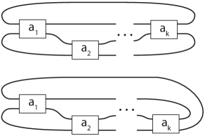
Figure 1. Rational knot/link $C(a_{1},a_{2},\ldots,a_{k})$. The upper/lower one corresponds to odd/even $k$.

A non-trivial group $G$ is left orderable if there is a total ordering $<$ on $G$ such that $g<h$ implies $fg<fh$ for every $f,g,h\in G$. A motivation for studying left orderable groups in topology is a conjectured connection with L-spaces. An L-space is a rational homology sphere $M$ with rank of $\mathrm{\widehat{HF}}(M)$ equal to $|H_{1}(M,\mathbb{Z})|$ [OS]. The L-space conjecture of Boyer-Gordon-Watson [BGW] states that an irreducible rational homology 3-sphere is an L-space if and only if its fundamental group is not left orderable.

We consider cyclic branched covers of knots in $S^{3}$ and study the left orderability of their fundamental groups. A sufficient condition for the fundamental group of the $r$-th cyclic branched cover of a prime knot to be left orderable was given in [BGW, Hu]. As an application, it was proved that for any rational knot $K$ with non-zero signature the fundamental group of the $r$-th cyclic branched cover of $K$ is left orderable for sufficiently large $r$, see [Hu, Tr1, Go]. For rational knots $C(k,2l)$, the left orderability of the fundamental groups of their cyclic branched covers was determined in [DPT, Tr2, Tu]. Moreover, Turner [Tu] also determined the left orderability of the fundamental groups of the cyclic branched covers of the rational knots $C(2n+1,2,2)$ for positive integers $n$.

In this paper, we will generalize Turner’s result to all rational knots $C(2n+1,2m,2)$ where $m$ and $n$ are non-zero integers. By studying real points on the nonabelian $\mathrm{SL_{2}}(\mathbb{C})$-character varieties of knot groups, we will prove the following.

Theorem 1.

The fundamental group of the $r$-th cyclic branched cover of the rational knot $C(2n+1,2m,2)$ is left orderable if

1. $r\geq 3$ when $n\geq 3$ or $n\leq-4$.

2. $r\geq 4$ when $n=2$ or $n=-3$.

3. $r\geq 5$ when $n=1$ and $m=1,2$, or $n=-2$ and $m=-1$.

4. $r\geq 6$ when $n=1$ and $m\geq 3$, or $n=-2$ and $m\leq-2$.

5. $r\geq 7$ when $n=1$ and $m\leq-4$ or $n=-2$ and $m\geq 6$.

6. $r\geq 8$ when $n=1$ and $m=-2,-3$.

7. $r\geq 9$ when $n=1$ and $m=-1$.

Figure 2. Rational knot $C(2n+1,2m,2)$.

This paper is organized as follows. In Section 2, we compute the nonabelian $\mathrm{SL_{2}}(\mathbb{C})$-character varieties of the rational knots $C(2n+1,2m,2)$. In Section 3, we prove some properties of the Chebychev polynomials of the second kind and character varieties of $C(2n+1,2m,2)$. Finally, in Section 4 we study real points on these character varieties and give a proof of Theorem 1.

2. Character varieties

In this section we will compute the nonabelian $\mathrm{SL_{2}}(\mathbb{C})$-character variety, i.e. the Riley polynomial, of $C(2n+1,2m,2)$ for non-zero integers $m$ and $n$.

For a knot $K$ in $S^{3}$ we denote by $G(K)$ the knot group of $K$, which is the fundamental group of the knot complement $X_{K}=S^{3}\setminus K$.

2.1. Knot group

Let $K_{n,m}$ denote the rational knot $C(2n+1,2m,2)$.

Proposition 2.1.

We have

$$G(K_{n,m})=\langle a,b\mid wa=bw\rangle$$

where $w=v^{n}(aba^{-1}b^{-1})^{m}ab$ and $v=(aba^{-1}b^{-1})^{m}a(aba^{-1}b^{-1})^{-m}b$.

Proof.

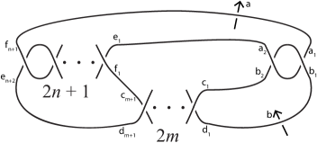
Figure 3. Generators $a,b$ of the knot group.

Starting from the right hand side of the knot diagram, we have the following two relations:

$$a_{1} =b_{1}a_{2}b_{1}^{-1},$$

$$b_{1} =a_{2}b_{2}a_{2}^{-1}.$$

In the middle section of $2m$ crossings we have, by induction,

$$c_{m+1} =(d_{1}c_{1}^{-1})^{-m}c_{1}(d_{1}c_{1}^{-1})^{m},$$

$$d_{m+1} =(d_{1}c_{1}^{-1})^{-m}d_{1}(d_{1}c_{1}^{-1})^{m}.$$

In the left hand section of $2n+1$ crossings we have, by induction,

$$e_{n+1} =(e_{1}f_{1})^{-n}e_{1}(e_{1}f_{1})^{n},$$

$$f_{n+1} =(e_{1}f_{1})^{-n}f_{1}(e_{1}f_{1})^{n}.$$

We have the following identifications:

$$a_{1}=f_{n+1},$$

$$e_{1}=a_{2},$$

$$f_{1}=c_{m+1},$$

$$d_{1}=b_{1},$$

$$c_{1}=b_{2}.$$

Let $a_{1}=a$ and $b_{1}=b$. Using the identity $a=f_{n+1}$ and the relations listed above, we have

$$a=(a_{2}c_{m+1})^{-n}(a^{-1}b^{-1}ab)^{-m}b^{-1}a^{-1}bab(a^{-1}b^{-1}ab)^{m}(a_{2}c_{m+1})^{n}.$$

This implies that $wa=bw$ where

$$w=ab(a^{-1}b^{-1})^{m}(a_{2}c_{m+1})^{n}.$$

Writing $a_{2}c_{m+1}$ in terms of $a$ and $b$, we have

$$a_{2}c_{m+1}=b^{-1}ab(a^{-1}b^{-1}ab)^{-m}b^{-1}a^{-1}bab(a^{-1}b^{-1}ab)^{m}.$$

Now we have

$$w =ab(a^{-1}b^{-1}ab)^{m}(b^{-1}ab(a^{-1}b^{-1}ab)^{-m}b^{-1}a^{-1}bab(a^{-1}b^{-1}ab)^{m})^{n}$$

$$=(ab(a^{-1}b^{-1}ab)^{m}b^{-1}ab(a^{-1}b^{-1}ab)^{-m}b^{-1}a^{-1}b)^{n}(aba^{-1}b^{-1})^{m}ab$$

$$=((aba^{-1}b^{-1})^{m}a(aba^{-1}b^{-1})^{-m}b)^{n}(aba^{-1}b^{-1})^{m}ab.$$

This completes the proof of Proposition 2.1. ∎

2.2. Nonabelian representations

Suppose $\rho\colon G(K_{n,m})\to\mathrm{SL}_{2}(\mathbb{C})$ is a nonabelian representation. Up to conjugation, we may assume that

(2.1) $$\rho(a)=\left[\begin{array}[]{cc}t&1\\ 0&t^{-1}\end{array}\right]\quad\text{and}\quad\rho(b)=\left[\begin{array}[]{cc}t&0\\ -u&t^{-1}\end{array}\right]$$

where $(t,u)\in\mathbb{C}^{2}$ satisfies the matrix equation $\rho(wa)=\rho(bw)$. It is known that this matrix equation is equivalent to a single polynomial equation $R_{K_{n,m}}(x,y)=0$, where $x=\operatorname{\mathrm{t}r}\rho(a)=t+t^{-1}$, $y=\operatorname{\mathrm{t}r}\rho(ab^{-1})=u+2$ and $R_{K}(x,y)$ is the Riley polynomial of a rational knot $K$, see [Ri]. This polynomial can be computed via the formula $R_{K}=w_{11}+(t^{-1}-t)w_{12}$, where $w_{ij}$ is the $ij$-th entry of the matrix $\rho(w)$. For the rational knot $K_{n,m}=C(2n+1,2m,2)$, the Riley polynomial can be described via the Chebyshev polynomials as follows.

Let $S_{k}(z)$ be the Chebyshev polynomials of the second kind defined by $S_{0}(z)=1$, $S_{1}(z)=z$ and $S_{k}(z)=zS_{k-1}(z)-S_{k-2}(z)$ for all integers $k$.

The following lemmas are elementary, see e.g [Tr3].

Lemma 2.2.

For any integer $k$ we have

$$S^{2}_{k}(z)+S^{2}_{k}(z)-zS_{k}(z)S_{k-1}(z)=S^{2}_{k}(z)-S_{k+1}(z)S_{k-1}(z)=1.$$

Lemma 2.3.

Suppose $V=\left[\begin{array}[]{cc}e&f\\ g&h\end{array}\right]\in\mathrm{SL}_{2}(\mathbb{C})$ and $z=\operatorname{\mathrm{t}r}V.$ For any integer $k$ we have

$$V^{k} = \left[\begin{array}[]{cc}S_{k}(z)-hS_{k-1}(z)&fS_{k-1}(z)\\ gS_{k-1}(z)&S_{k}(z)-eS_{k-1}(z)\end{array}\right].$$

Let $\alpha=\operatorname{\mathrm{t}r}\rho(aba^{-1}b^{-1})$ and $\beta=\operatorname{\mathrm{t}r}\rho(v)$.

Proposition 2.4.

We have

$$\alpha = y^{2}-x^{2}y+2x^{2}-2,$$

$$\beta = 2+(x^{2}-y-2)\big{(}S_{m}(\alpha)+(1-y)S_{m-1}(\alpha)\big{)}^{2}.$$

Proof.

By a direct calculation we have

$$\rho(aba^{-1}b^{-1})=\left[\begin{array}[]{cc}u^{2}-u(t^{2}+t^{-2}-1)+1&t(u-t^{2}+1)\\ t^{-1}u(u-t^{-2}+1)&u+1\\ \end{array}\right].$$

Hence

$$\alpha=\operatorname{\mathrm{t}r}\rho(aba^{-1}b^{-1})=u^{2}-u(t^{2}+t^{-2}-2)+2.$$

By Lemma 2.3 we have $\rho((aba^{-1}b^{-1})^{m})=\left[\begin{array}[]{cc}e&f\\ g&h\\ \end{array}\right]$ where

$$e = S_{m}(\alpha)-(u+1)S_{m-1}(\alpha),$$

$$f = t(u-t^{2}+1)S_{m-1}(\alpha),$$

$$g = t^{-1}u(u-t^{-2}+1)S_{m-1}(\alpha),$$

$$h = S_{m}(\alpha)-\big{(}u^{2}-u(t^{2}+t^{-2}-1)+1\big{)}S_{m-1}(\alpha).$$

By a direct calculation we have

$$\rho(v) = \rho\big{(}(aba^{-1}b^{-1})^{m}a(aba^{-1}b^{-1})^{-m}b\big{)}$$

$$= \left[\begin{array}[]{cc}e&f\\ g&h\\ \end{array}\right]\left[\begin{array}[]{cc}t&1\\ 0&t^{-1}\end{array}\right]\left[\begin{array}[]{cc}h&-f\\ -g&e\\ \end{array}\right]\left[\begin{array}[]{cc}t&0\\ -u&t^{-1}\end{array}\right]=\left[\begin{array}[]{cc}v_{11}&v_{12}\\ v_{21}&v_{22}\\ \end{array}\right]$$

where

$$v_{11} = t^{2}eh-teg-fg+ue((t-t^{-1})f-e),$$

$$v_{12} = -t^{-1}e((t-t^{-1})f-e),$$

$$v_{21} = tg((t-t^{-1})h-g)+u(tfg-t^{-1}eh-eg),$$

$$v_{22} = t^{-1}eg+t^{-2}eh-fg.$$

With $\beta=\operatorname{\mathrm{t}r}\rho(v)=v_{11}+v_{22}$ we have

$$\beta = (t^{2}+t^{-2})eh-(t-t^{-1})eg-2fg+ue((t-t^{-1})f-e)$$

$$= 2(eh-fg)+e\big{[}(t^{2}+t^{-2}-2)h+(t-t^{-1})(uf-g)-ue\big{]}.$$

Since $eh-fg=1$ and $uf-g=(t-t^{-1})u(u-t^{2}-t^{-2})S_{m-1}(\alpha)=(t-t^{-1})(e-h),$ we obtain

$$\beta=2+(t^{2}+t^{-2}-2-u)e^{2}=2+(t^{2}+t^{-2}-2-u)\big{(}S_{m}(\alpha)-(u+1)S_{m-1}(\alpha)\big{)}^{2}.$$

Finally, since $t^{2}+t^{-2}=x^{2}-2$ and $u=y-2$, Proposition 2.4 follows. ∎

Let $R_{n,m}(x,y)$ denote the Riley polynomial of $C(2n+1,2m,2)$.

Proposition 2.5.

We have

$$R_{n,m}(x,y)=\big{(}(x^{2}-y-1)S_{m}(\alpha)-S_{m-1}(\alpha)\big{)}S_{n}(\beta)-\big{(}(x^{2}-y-1)S_{m-1}(\alpha)-S_{m-2}(\alpha)\big{)}S_{n-1}(\beta).$$

Proof.

By Lemma 2.3 we have $\rho(v^{n})=\left[\begin{array}[]{cc}p&q\\ r&s\\ \end{array}\right]$ where

$$p = S_{n}(\beta)-v_{22}S_{n-1}(\beta),\qquad q=v_{12}S_{n-1}(\beta),$$

$$r = v_{21}S_{n-1}(\beta),\qquad\qquad\quad\,\,\,\,s=S_{n}(\beta)-v_{11}S_{n-1}(\beta).$$

By a direct calculation we have

$$\rho(w) = \rho(v^{n}(aba^{-1}b^{-1})^{m}ab)$$

$$= \left[\begin{array}[]{cc}p&q\\ r&s\\ \end{array}\right]\left[\begin{array}[]{cc}e&f\\ g&h\\ \end{array}\right]\left[\begin{array}[]{cc}t&1\\ 0&t^{-1}\end{array}\right]\left[\begin{array}[]{cc}t&0\\ -u&t^{-1}\end{array}\right]=\left[\begin{array}[]{cc}w_{11}&w_{12}\\ w_{21}&w_{22}\\ \end{array}\right]$$

where

$$w_{11} = (t^{2}-u)(ep+gq)-t^{-1}u(fp+hq),$$

$$w_{12} = t^{-2}(fp+hq)+t^{-1}(ep+gq),$$

$$w_{21} = (t^{2}-u)(er+gs)-t^{-1}u(fr+hs),$$

$$w_{22} = t^{-2}(fr+hs)+t^{-1}(er+gs).$$

The Riley polynomial is

$$R_{n,m}=w_{11}+(t^{-1}-t)w_{12}=(t^{2}+t^{-2}-u-1)(ep+gq)-t^{-1}(u+1-t^{-2})(fp+hq).$$

Since $p=S_{n}(\beta)-v_{22}S_{n-1}(\beta)$ and $q=v_{12}S_{n-1}(\beta)$ we have

$$ep+gq = e(S_{n}(\beta)-v_{22}S_{n-1}(\beta))+gv_{12}S_{n-1}(\beta)=eS_{n}(\beta)+(gv_{12}-ev_{22})S_{n-1}(\beta),$$

$$fp+hq = f(S_{n}(\beta)-v_{22}S_{n-1}(\beta))+hv_{12}S_{n-1}(\beta)=fS_{n}(\beta)+(hv_{12}-fv_{22})S_{n-1}(\beta).$$

With $v_{22}=t^{-1}eg+t^{-2}eh-fg$ and $v_{12}=-t^{-1}e((t-t^{-1})f-e)$, we have

$$gv_{12}-ev_{22} = t^{-2}e(fg-eh)=-t^{-2}e,$$

$$hv_{12}-fv_{22} = t^{-1}(eh-fg)(ft-e)=t^{-1}(ft-e).$$

Hence

$$R_{n,m} = \big{[}(t^{2}+t^{-2}-u-1)e-t^{-1}(u+1-t^{-2})f\big{]}S_{n}(\beta)$$

$$\qquad-\,t^{-2}\big{[}(t^{2}+t^{-2}-u-1)e-(u+1-t^{-2})(ft-e)\big{]}S_{n-1}(\beta)$$

$$= \big{[}(t^{2}+t^{-2}-u-1)e-t^{-1}(u+1-t^{-2})f\big{]}S_{n}(\beta)$$

$$\qquad-\,\big{[}e-t^{-1}(u+1-t^{-2})f\big{]}S_{n-1}(\beta).$$

Then, with $e=S_{m}(\alpha)-(u+1)S_{m-1}(\alpha)$ and $f=t(u-t^{2}+1)S_{m-1}(\alpha)$, we obtain

$$R_{n,m} = \big{[}(t^{2}+t^{-2}-u-1)S_{m}(\alpha)-S_{m-1}(\alpha)\big{]}S_{n}(\beta)$$

$$\qquad+\,\big{[}(u^{2}-(t^{2}+t^{-2}-3)u+t^{2}+t^{-2}-3)S_{m-1}(\alpha)-S_{m}(\alpha)\big{]}S_{n-1}(\beta).$$

Since $\alpha=u^{2}-u(t^{2}+t^{-2}-2)+2$ we have

$$(u^{2}-(t^{2}+t^{-2}-3)u-t^{2}-t^{-2}+3)S_{m-1}(\alpha)-S_{m}(\alpha)$$

$$= (\alpha+u-t^{2}-t^{-2}+1)S_{m-1}(\alpha)-S_{m}(\alpha)$$

$$= S_{m-2}(\alpha)-(t^{2}+t^{-2}-u-1)S_{m-1}(\alpha).$$

The formula for $R_{n,m}(x,y)$ follows, since $t^{2}+t^{-2}=x^{2}-2$ and $u=y-2$. ∎

3. Properties of the Riley polynomial

In this section we will prove some properties of the Chebychev polynomials of the second kind and Riley polynomials of the rational knots $C(2n+1,2m,2)$. We will make use of these properties in Section 4.

3.1. Chebychev polynomials

Recall that $S_{k}(z)$’s are the Chebyshev polynomials defined by $S_{0}(z)=1$, $S_{1}(z)=z$ and $S_{k}(z)=zS_{k-1}(z)-S_{k-2}(z)$ for all integers $k$.

Lemma 3.1.

The followings hold true:

1. For $k\geq 0$, the polynomial $S_{k}(z)$ has degree $k$ and leading term $z^{k}$.

2. For $k\geq 1$ we have $S_{-k}(z)=-S_{k-2}(z)$.

3. $S_{k}(\pm 2)=(\pm 1)^{k}(k+1)$ and $S_{k}(z)=(t^{k+1}-t^{-k-1})/(t-t^{-1})$ if $z=t+t^{-1}\not=\pm 2$. In particular we have $S_{k}(2\cos\theta)=\frac{\sin(k+1)\theta}{\sin\theta}$ for $\theta\in\mathbb{R}\setminus\mathbb{Z}\pi$.

Proof.

All the equalities in the lemma can be proved by induction on $k\geq 0$. For the last equality, note that $2\cos\theta=e^{i\theta}+e^{-i\theta}$. ∎

Lemma 3.2.

Suppose $k\geq 1$. Then the polynomial $S_{k}(z)-S_{k-1}(z)=0$ has $k$ roots given by $z=2\cos\theta_{j}$ where $\theta_{j}=\frac{(2j-1)\pi}{2k+1}$ for $1\leq j\leq k$. Moreover, at $z=2\cos\theta_{j}$ we have $(-1)^{j+1}S_{k}(z)>0$.

Proof.

By Lemma 3.1(3), at $z=2\cos\theta_{j}$ we have

$$S_{k}(z) =\frac{\sin(k+1)\theta_{j}}{\sin\theta_{j}}=\frac{\sin((j-\frac{1}{2})\pi+\frac{\theta_{j}}{2})}{\sin\theta_{j}}=\frac{(-1)^{j+1}\cos\frac{\theta_{j}}{2}}{\sin\theta_{j}}=\frac{(-1)^{j+1}}{2\sin\frac{\theta_{j}}{2}},$$

$$S_{k-1}(z) =\frac{\sin k\theta_{j}}{\sin\theta_{j}}=\frac{\sin((j-\frac{1}{2})\pi-\frac{\theta_{j}}{2})}{\sin\theta_{j}}=\frac{(-1)^{j+1}\cos\frac{\theta_{j}}{2}}{\sin\theta_{j}}=\frac{(-1)^{j+1}}{2\sin\frac{\theta_{j}}{2}}.$$

This implies that $S_{k}(z)=S_{k-1}(z)$ and $(-1)^{j+1}S_{k}(z)>0$. Hence the polynomial $S_{k}(z)-S_{k-1}(z)$ has at least $k$ roots given by $z=2\cos\theta_{j}$ for $1\leq j\leq k$. Since the degree of $S_{k}(z)-S_{k-1}(z)$ is exactly $k$, those are all the roots. ∎

3.2. Riley poynomial

Recall from Propositions 2.4 and 2.5 that

$$\alpha = y^{2}-x^{2}y+2x^{2}-2,$$

$$\beta = 2+(x^{2}-y-2)\big{(}S_{m}(\alpha)+(1-y)S_{m-1}(\alpha)\big{)}^{2}.$$

and

$$R_{n,m}(x,y)=\big{(}(x^{2}-y-1)S_{m}(\alpha)-S_{m-1}(\alpha)\big{)}S_{n}(\beta)-\big{(}(x^{2}-y-1)S_{m-1}(\alpha)-S_{m-2}(\alpha)\big{)}S_{n-1}(\beta).$$

Lemma 3.3.

For any fixed number $x\in\mathbb{R}$, we have

$$\lim_{y\to\infty}(-1)^{n}R_{n,m}(x,y)=\begin{cases}-\infty&\mbox{if }n\geq 1,m\geq 1,\\ \infty&\mbox{if }n\geq 1,m\leq-1,\\ \infty&\mbox{if }n\leq-1,m\geq 1,\\ -\infty&\mbox{if }n\leq-1,m\leq-1.\end{cases}$$

Proof.

We will prove the lemma for the case $n\geq 1$. The case $n\leq-1$ is proved similarly.

By Lemma 3.1(1), when $k\geq 0$ the leading term of $S_{k}(z)$ is $z^{k}$. Moreover, by Lemma 3.1(2) we have $S_{-1}(z)=0$ and $S_{-k}(z)=-S_{k-2}(z)$ for $k\geq 2$. Hence when $k\geq 2$ the leading term of $S_{-k}(z)$ is $-z^{k-2}$.

Fix $x\in\mathbb{R}$. Since the leading term of $\alpha$ is $y^{2}$, we see that the leading term of $(x^{2}-y-1)S_{m}(\alpha)-S_{m-1}(\alpha)$ is $\begin{cases}-y^{2m+1}&\mbox{if }m\geq 1,\\ y^{-2(m+1)}&\mbox{if }m\leq-1.\end{cases}$

Similarly, the leading term of $(x^{2}-y-1)S_{m-1}(\alpha)-S_{m-2}(\alpha)$ is $\begin{cases}-y^{2m-1}&\mbox{if }m\geq 1,\\ y^{-2m}&\mbox{if }m\leq-1,\end{cases}$ and the leading term of $\beta=2+(x^{2}-y-2)\big{(}S_{m}(\alpha)+(1-y)S_{m-1}(\alpha)\big{)}^{2}$ is $-y^{|4m+1|}$.

Since $n\geq 1$, the leading term of $S_{n}(\beta)$ is equal to that of $\beta^{n}$, which is $(-y^{|4m+1|})^{n}$. Similarly, the leading term of $S_{n-1}(\beta)$ is equal to that of $\beta^{n-1}$, which is $(-y^{|4m+1|})^{n-1}$.

If $m\geq 1$, the leading term of $R_{n,m}(x,y)$ is equal to that of $\big{(}(x^{2}-y-1)S_{m}(\alpha)-S_{m-1}(\alpha)\big{)}S_{n}(\beta)$, which is $-y^{2m+1}(-y^{4m+1})^{n}=(-1)^{n+1}y^{2m+1+(4m+1)n}$.

If $m\leq-1$, the leading term of $R_{n,m}(x,y)$ is equal to that of $\big{(}(x^{2}-y-1)S_{m}(\alpha)-S_{m-1}(\alpha)\big{)}S_{n}(\beta)$, which is $y^{-2(m+1)}(-y^{-4m-1})^{n}=(-1)^{n}y^{-2(m+1)+(-4m-1)n}$.

This completes the proof of the lemma for the case $n\geq 1$. ∎

Lemma 3.4.

Suppose $S_{n}(\beta)=S_{n-1}(\beta)$. Then

$$R_{n,m}(x,y)=(x^{2}-y-2)[S_{m}(\alpha)+(1-y)S_{m-1}(\alpha)]S_{n}(\beta).$$

Proof.

If $S_{n}(\beta)=S_{n-1}(\beta)$ then

$$R_{n,m}(x,y) =[(x^{2}-y-1)S_{m}(\alpha)-S_{m-1}(\alpha)-(x^{2}-y-1)S_{m-1}(\alpha)+S_{m-2}(\alpha)]S_{n}(\beta)$$

$$=[(x^{2}-y-1)(S_{m}(\alpha)-S_{m-1}(\alpha))+(\alpha-1)S_{m-1}(\alpha)-S_{m}(\alpha)]S_{n}(\beta)$$

$$=[(x^{2}-y-1)(S_{m}(\alpha)-S_{m-1}(\alpha))$$

$$\hskip 85.35826pt-(\alpha-1)(S_{m}(\alpha)-S_{m-1}(\alpha))+(\alpha-2)S_{m}(\alpha)]S_{n}(\beta)$$

$$=[(\alpha-2)S_{m}(\alpha)+(x^{2}-y-\alpha)(S_{m}(\alpha)-S_{m-1}(\alpha))]S_{n}(\beta).$$

Since $\alpha=y^{2}-x^{2}y+2x^{2}-2$, we have $\alpha-2=(y-2)(y+2-x^{2})$ and $x^{2}-y-\alpha=(1-y)(y+2-x^{2})$. Hence

$$R_{n,m}(x,y) =(y+2-x^{2})[(y-2)S_{m}(\alpha)+(1-y)(S_{m}(\alpha)-S_{m-1}(\alpha))]$$

$$=(x^{2}-y-2)[S_{m}(\alpha)+(1-y)S_{m-1}(\alpha)]S_{n}(\beta).$$

∎

Lemma 3.5.

Suppose $y=2$. Then $\alpha=2$, $\beta=x^{2}-2$ and

$$R_{n,m}(x,y)=m(\beta-2)(S_{n}(\beta)-S_{n-1}(\beta))+S_{n+1}(\beta)-S_{n}(\beta).$$

Moreover, if we also have $x=2\cos\theta$ for some $\theta\in\mathbb{R}\setminus\mathbb{Z}\frac{\pi}{2}$ then

$$R_{n,m}(x,y)=m(2\cos 2\theta-2)\frac{\cos(2n+1)\theta}{\cos\theta}+\frac{\cos(2n+3)\theta}{\cos\theta}.$$

Proof.

Since $y=2$ we have $\alpha=y^{2}-x^{2}y+2x^{2}-2=2$ and so $S_{k}(\alpha)=k+1$ for all $k\in\mathbb{Z}$. This implies that $\beta=2+(x^{2}-y-2)\big{(}S_{m}(\alpha)+(1-y)S_{m-1}(\alpha)\big{)}^{2}=x^{2}-2$ and

$$R_{n,m}(x,y) =[(x^{2}-3)S_{m}(\alpha)-S_{m-1}(\alpha)]S_{n}(\beta)-[(x^{2}-3)S_{m-1}(\alpha)-S_{m-2}(\alpha)]S_{n-1}(\beta)$$

$$=[(\beta-1)(m+1)-m]S_{n}(\beta)-[(\beta-1)m-(m-1)]S_{n-1}(\beta)$$

$$=m(\beta-2)(S_{n}(\beta)-S_{n-1}(\beta))+(\beta-1)S_{n}(\beta)-S_{n-1}(\beta)$$

$$=m(\beta-2)(S_{n}(\beta)-S_{n-1}(\beta))+S_{n+1}(\beta)-S_{n}(\beta).$$

If we also have $x=2\cos\theta$ for some $\theta\in\mathbb{R}\setminus\mathbb{Z}\frac{\pi}{2}$ then $\beta=x^{2}-2=2\cos 2\theta$. Since $2\theta\in\mathbb{R}\setminus\mathbb{Z}\pi$, by Lemma 3.1(3) we have $S_{k}(\beta)=\frac{\sin(2k+2)\theta}{\sin 2\theta}$ for all $k\in\mathbb{Z}$. Hence

$$R_{n,m}(x,y) =m(2\cos 2\theta-2)\frac{\sin(2n+2)\theta-\sin 2n\theta}{\sin 2\theta}+\frac{\sin(2n+4)\theta-\sin(2n+2)\theta}{\sin 2\theta}$$

$$=m(2\cos 2\theta-2)\frac{\cos(2n+1)\theta}{\cos\theta}+\frac{\cos(2n+3)\theta}{\cos\theta}.$$

∎

4. Left orderability of cyclic branched covers

In this section we will study real roots of the Riley polynomial of the rational knot $C(2n+1,2m,2)$. We then use the properties of real roots to make a conclusion about the left orderability of the fundamental groups of the cyclic branched covers of $C(2n+1,2m,2)$.

4.1. Real roots of the Riley polynomial

There are four cases to consider: when both $n$ and $m$ are the same sign and when $n$ and $m$ are opposite in sign. We will carefully study real roots of the Riley polynomial for the cases $n\geq 1$, $m\geq 1$ and $n\geq 2$, $m\leq-1$. The other two cases are similar. Additionally, the cases $n=1$, $m\leq-1$ and $n=-2$, $m\geq 1$ differ slightly from the others. So we will consider them separately.

4.1.1.

Case $\bf{1}$: $n\geq 1$, $m\geq 1$.

Lemma 4.1.

Suppose $y>2$ and $x\in\mathbb{R}$ satisfies $x^{2}\leq 4$. Then

$$S_{m}(\alpha)+(1-y)S_{m-1}(\alpha)>0.$$

Proof.

Let $u=y-2$, then $\alpha=2+u^{2}+(4-x^{2})u$. Since $u>0$ and $4\geq x^{2}$, we have $\alpha\geq 2+u^{2}:=\alpha_{0}.$ Choose $v>1$ such that $u=v-v^{-1}$, and so $\alpha_{0}=v^{2}+v^{-2}$. Then

$$\frac{S_{m}(\alpha_{0})}{S_{m-1}(\alpha_{0})}-u-1 = \frac{v^{2m+2}-v^{-2m-2}}{v^{2m}-v^{-2m}}-(v-v^{-1})-1$$

$$= \frac{(v^{2}-1)(v+1+v^{1+4m}(v-1))}{v^{2}(v^{4m}-1)}>0.$$

Since $S_{m}(\alpha)/S_{m-1}(\alpha)$ is increasing in $\alpha\in(2,\infty)$ and $\alpha\geq\alpha_{0}$, we have

$$\frac{S_{m}(\alpha)}{S_{m-1}(\alpha)}\geq\frac{S_{m}(\alpha_{0})}{S_{m-1}(\alpha_{0})}>u+1=y-1.$$

Therefore $S_{m}(\alpha)+(1-y)S_{m-1}(\alpha)>0$. ∎

Proposition 4.2.

Suppose $x\in\mathbb{R}$ satisfies $4\geq x^{2}>2+2\cos\frac{(2n-1)\pi}{2n+1}$. Then $R_{n,m}(x,y)=0$ has at least one real solution $y>2$.

Proof.

By Lemma 3.3 we have $(-1)^{n}R_{n,m}(x,y)\to-\infty$ as $y\to\infty$. To prove the proposition, it suffices to show that there exists $y_{0}\geq 2$ such that $(-1)^{n}R_{n,m}(x,y_{0})>0$.

If we let $y=2$, then by Lemma 3.5 we have $\beta=x^{2}-2>2\cos\frac{(2n-1)\pi}{2n+1}$. Since the leading term of $\beta$ is $-y^{4m+1}$, we have $\beta\to-\infty$ as $y\to\infty$. Hence there exists $y_{0}\in(2,\infty)$ such that $\beta=2\cos\frac{(2n-1)\pi}{2n+1}$. Lemma 3.2 implies that $S_{n}(\beta)=S_{n-1}(\beta)$ and $(-1)^{n+1}S_{n}(\beta)>0$. Then by Lemma 3.4 we have

$$R_{n,m}(x,y_{0})=(x^{2}-y_{0}-2)[S_{m}(\alpha)+(1-y_{0})S_{m-1}(\alpha)]S_{n}(\beta).$$

Since $y_{0}>2$ and $x\in\mathbb{R}$ satisfies $4\geq x^{2}$, by Lemma 4.1 we have $S_{m}(\alpha)+(1-y_{0})S_{m-1}(\alpha)>0$. Note that $x^{2}-y_{0}-2<0$ and the sign of $S_{n}(\beta)$ is $(-1)^{n+1}$. So the sign of $R_{n,m}(x,y_{0})$ is $(-1)^{n}$, which means that $(-1)^{n}R_{n,m}(x,y_{0})>0$. ∎

If we let $x=2\cos\frac{\pi}{r}$ for some integer $r\geq 2$, then the condition $x^{2}>2+2\cos\frac{\pi(2n-1)}{2n+1}$ is equivalent to $\cos\frac{2\pi}{r}>\cos\frac{\pi(2n-1)}{2n+1}$ and so $r>\frac{2(2n+1)}{2n-1}=2+\frac{4}{2n-1}$. This gives the following lower bound for $r$:

• $r\geq 3$ if $n\geq 3$.

• $r\geq 4$ if $n=2$.

• $r\geq 7$ if $n=1$.

In the case $n=1$, we can slightly improve the lower bound for $r$.

Proposition 4.3.

$R_{1,m}(2\cos\frac{\pi}{r},y)=0$ has at least one real solution $y>2$ in the following cases:

1. $r=5,6$ when $m=1,2$.

2. $r=6$ when $m\geq 3$.

Proof.

Since $m\geq 1$, by Lemma 3.3 we have $R_{1,m}(2\cos\frac{\pi}{r},y)\to\infty$ as $y\to\infty$. To prove the proposition, it suffices to check that $R_{1,m}(2\cos\frac{\pi}{r},2)<0$.

By Lemma 3.5 we have $R_{1,m}(2\cos\frac{\pi}{r},2)=m(2\cos\frac{2\pi}{r}-2)\frac{\cos\frac{3\pi}{r}}{\cos\frac{\pi}{r}}+\frac{\cos\frac{5\pi}{r}}{\cos\frac{\pi}{r}}$.

If $r=6$, then $R_{1,m}(2\cos\frac{\pi}{r},2)=-1<0$.

If $r=5$, then by a direct calculation we have

$$R_{1,m}(2\cos\frac{\pi}{r},2)=(5-2\sqrt{5})m+1-\sqrt{5}=\begin{cases}6-3\sqrt{5}&\mbox{if }m=1,\\ 11-5\sqrt{5}&\mbox{if }m=2,\end{cases}$$

which is negative when $m=1,2$. ∎

4.1.2.

Case $\bf{2}$: $n\geq 2$, $m\leq-1$.

Proposition 4.4.

Suppose $x\in\mathbb{R}$ satisfies $4\geq x^{2}>2+2\cos\frac{(2n-3)\pi}{2n+1}$. Then $R_{n,m}(x,y)=0$ has at least one real solution $y>2$.

Proof.

By Lemma 3.3 we have $(-1)^{n}R_{n,m}(x,y)\to\infty$ as $y\to\infty$. To prove the proposition, it suffices to show that there exists $y_{0}\geq 2$ such that $(-1)^{n}R_{n,m}(x,y_{0})<0$.

If we let $y=2$, then by Lemma 3.5 we have $\beta=x^{2}-2>2\cos\frac{(2n-3)\pi}{2n+1}$. Since the leading term of $\beta$ is $-y^{|4m+1|}$, we have $\beta\to-\infty$ as $y\to\infty$. Hence there exists $y_{0}>2$ such that $\beta=2\cos\frac{(2n-3)\pi}{2n+1}$. Lemma 3.2 implies that $S_{n}(\beta)=S_{n-1}(\beta)$ and $(-1)^{n}S_{n}(\beta)>0$. Then by Lemma 3.4 we have

$$R_{n,m}(x,y_{0}) =(x^{2}-y_{0}-2)[S_{m}(\alpha)+(1-y_{0})S_{m-1}(\alpha)]S_{n}(\beta)$$

$$=(x^{2}-y_{0}-2)[(y_{0}-1)S_{-m-1}(\alpha)-S_{-m-2}(\alpha)]S_{n}(\beta).$$

Since $y_{0}>2$ and $x^{2}\leq 4$, we have $\alpha=2+(y_{0}-2)(y_{0}+2-x^{2})>2$. This implies that

$$(y_{0}-1)S_{-m-1}(\alpha)-S_{-m-2}(\alpha)>S_{-m-1}(\alpha)-S_{-m-2}(\alpha)>0.$$

So the sign of $R_{n,m}(x,y_{0})$ is $(-1)^{n+1}$, which means that $(-1)^{n}R_{n,m}(x,y_{0})<0$. ∎

If we let $x=2\cos\frac{\pi}{r}$ for some integer $r\geq 2$, then the condition $x^{2}>2+2\cos\frac{\pi(2n-3)}{2n+1}$ becomes $\cos\frac{2\pi}{r}>\cos\frac{\pi(2n-3)}{2n+1}$ and so $r>\frac{2(2n+1)}{2n-3}=2+\frac{8}{2n-3}$. This gives the following lower bound for $r$:

• $r\geq 3$ if $n\geq 6$.

• $r\geq 4$ if $n=4,5$.

• $r\geq 5$ if $n=3$.

• $r\geq 11$ if $n=2$.

In the cases $n=2,3,4,5$, we can slightly improve these lower bounds.

Proposition 4.5.

$R_{n,m}(2\cos\frac{\pi}{r},y)=0$ has at least one real solution $y>2$ in the following cases:

1. $r=3$ when $n=4,5$.

2. $r=3,4$ when $n=3$.

3. $4\leq r\leq 10$ when $n=2$.

Proof.

Since $m\leq-1$, by Lemma 3.3 we have $(-1)^{n}R_{n,m}(2\cos\frac{\pi}{r},y)\to\infty$ as $y\to\infty$. To prove the proposition, it suffices to check that $(-1)^{n}R_{n,m}(2\cos\frac{\pi}{r},2)<0$.

By Lemma 3.5 we have

$$R_{n,m}(2\cos\frac{\pi}{r},2)=m(2\cos\frac{2\pi}{r}-2)\frac{\cos\frac{(2n+1)\pi}{r}}{\cos\frac{\pi}{r}}+\frac{\cos\frac{(2n+3)\pi}{r}}{\cos\frac{\pi}{r}}.$$

If $r=3$ then $R_{n,m}(2\cos\frac{\pi}{r},2)=-6m\cos\frac{(2n+1)\pi}{3}+2\cos\frac{(2n+3)\pi}{3}=\begin{cases}-2-3m&\mbox{if }n=3,\\ 1+6m&\mbox{if }n=4,\\ 1-3m&\mbox{if }n=5,\end{cases}$ which has the sign $(-1)^{n+1}$ when $n=3,4,5$.

If $r=4$ then $R_{n,m}(2\cos\frac{\pi}{r},2)=-2\sqrt{2}m\cos\frac{(2n+1)\pi}{4}+\sqrt{2}\cos\frac{(2n+3)\pi}{4}=\begin{cases}1+2m&\mbox{if }n=2,\\ 1-2m&\mbox{if }n=3,\end{cases}$ which has the sign $(-1)^{n+1}$ when $n=2,3$.

If $n=2$ and $5\leq r\leq 10$ then by direct calculations we have

$$R_{n,m}(2\cos\frac{\pi}{r},2) = m(2\cos\frac{2\pi}{r}-2)\frac{\cos\frac{5\pi}{r}}{\cos\frac{\pi}{r}}+\frac{\cos\frac{7\pi}{r}}{\cos\frac{\pi}{r}}$$

$$\leq -(2\cos\frac{2\pi}{r}-2)\frac{\cos\frac{5\pi}{r}}{\cos\frac{\pi}{r}}+\frac{\cos\frac{7\pi}{r}}{\cos\frac{\pi}{r}}$$

$$< 0.$$

So $R_{n,m}(2\cos\frac{\pi}{r},2)$ has the sign $(-1)^{n+1}$. ∎

The cases $n\leq-3$, $m\geq 1$ and $n\leq-2$, $m\leq-1$ can be proved in a similar way as Cases $1$ and $2$ above. However, this method of proof does not include the cases $n=1$, $m\leq-1$ and $n=-2$, $m\geq 1$. We will consider them next.

4.1.3.

Case $\bf{3}$: $n=1$, $m\leq-1$.

Proposition 4.6.

$R_{1,m}(2\cos\frac{\pi}{r},y)=0$ has at least one real solution $y>2$ in the following cases:

1. $r\geq 7$ when $m\leq-4$.

2. $r\geq 8$ when $m=-2,-3$.

3. $r\geq 9$ when $m=-1$.

Proof.

Since $m\leq-1$, by Lemma 3.3 we have $R_{1,m}(2\cos\frac{\pi}{r},y)\to-\infty$ as $y\to\infty$. To prove the proposition, it suffices to check that $R_{1,m}(2\cos\frac{\pi}{r},2)>0$.

By Lemma 3.5 we have

$$R_{1,m}(2\cos\frac{\pi}{r},2) =m(\beta-2)(S_{1}(\beta)-S_{0}(\beta))+S_{2}(\beta)-S_{1}(\beta)$$

$$=m(\beta-2)(\beta-1)+\beta^{2}-\beta-1,$$

where $\beta=x^{2}-2=2\cos\frac{2\pi}{r}$.

For $m\leq-2$, the inequality $R_{1,m}(2\cos\frac{\pi}{r},2)>0$ is equivalent to

$$\frac{3m+1-\sqrt{m^{2}+2m+5}}{2(m+1)}>\beta=2\cos\frac{2\pi}{r}>\frac{3m+1+\sqrt{m^{2}+2m+5}}{2(m+1)}.$$

Note that $\frac{3m+1-\sqrt{m^{2}+2m+5}}{2(m+1)}>\frac{3m+3-\sqrt{m^{2}+2m+1}}{2(m+1)}=2$. Hence we only need

$$2\cos\frac{2\pi}{r}>\frac{3m+1+\sqrt{m^{2}+2m+5}}{2(m+1)}=\frac{3}{2}-\left(\frac{1}{m+1}+\sqrt{\frac{1}{4}+\frac{1}{(m+1)^{2}}}\,\right).$$

For $m=-2$, we have $2\cos\frac{2\pi}{r}>\frac{5-\sqrt{5}}{2}$ if $r\geq 8$.

For $m=-3$, we have $2\cos\frac{2\pi}{r}>1-\frac{\sqrt{2}}{4}$ if $r\geq 8$.

For $m\leq-4$, we have

$$\frac{1}{m+1}+\sqrt{\frac{1}{4}+\frac{1}{(m+1)^{2}}}=\frac{1/4}{\frac{1}{-(m+1)}+\sqrt{\frac{1}{4}+\frac{1}{(m+1)^{2}}}}\geq\frac{1/4}{\frac{2+\sqrt{13}}{6}}=\frac{\sqrt{13}-2}{6}.$$

So we only need $2\cos\frac{2\pi}{r}>\frac{3}{2}-\frac{\sqrt{13}-2}{6}$. This holds true if $r\geq 7$.

Finally, when $m=-1$ we have $R_{1,m}(2\cos\frac{\pi}{r},2)=4\cos\frac{2\pi}{r}-3<0$ if $r\geq 9$. ∎

4.1.4.

Case $\bf{4}$: $n=-2$, $m\geq 1$.

Lemma 4.7.

Suppose $m\geq 1$ and $x\in\mathbb{R}$ such that $4\geq x^{2}>2+\frac{2m}{m+1}$. Then there exists a unique $y_{0}>2$ such that $S_{m}(\alpha)+(1-y_{0})S_{m-1}(\alpha)=1$.

Proof.

Consider $y>2$. Note that $S_{m}(\alpha)+(1-y)S_{m-1}(\alpha)>0$ (by Lemma 4.1) and $S^{2}_{m}(\alpha)+S^{2}_{m-1}(\alpha)-\alpha S_{m}(\alpha)S_{m-1}(\alpha)=1$ (by Lemma 2.2). This implies that the equation $S_{m}(\alpha)+(1-y_{0})S_{m-1}(\alpha)=1$ is equivalent to

$$(S_{m}(\alpha)+(1-y)S_{m-1}(\alpha))^{2}=S^{2}_{m}(\alpha)+S^{2}_{m-1}(\alpha)-\alpha S_{m}(\alpha)S_{m-1}(\alpha).$$

With $\alpha=2+(y-2)(2+y-x^{2})$, the above equation becomes $(y-2)S_{m-1}(y)[(x^{2}-y)S_{m}(\alpha)-yS_{m-1}(\alpha)]=0$, i.e. $(x^{2}-y)S_{m}(\alpha)-yS_{m-1}(\alpha)=0$. We have shown that for $y>2$, the equation $S_{m}(\alpha)+(1-y)S_{m-1}(\alpha)=1$ is equivalent to $(x^{2}-y)S_{m}(\alpha)-yS_{m-1}(\alpha)=0$, which is also equivalent to $P(y):=(y^{2}-yx^{2}+x^{2})S_{m-1}(\alpha)+y-x^{2}=0$.

It is easy to see that $P(y)$ is an increasing function on $(2,\infty)$ and $\lim_{y\to\infty}P(y)=\infty$. Moreover $P(2)=(4-x^{2})m+2-x^{2}=2m-(x^{2}-2)(m+1)<0$, since $x^{2}-2>\frac{2m}{m+1}$. Hence there exists a unique $y_{0}>2$ such that $S_{m}(\alpha)+(1-y)S_{m-1}(\alpha)=1$. ∎

Proposition 4.8.

$R_{-2,m}(2\cos\frac{\pi}{r},y)=0$ has at least one real solution $y>2$ if $r\geq 7$ and $m\geq 6$.

Proof.

Suppose $r\geq 7$ and $m\geq 6$. By Lemma 3.3 we have $R_{-2,m}(2\cos\frac{\pi}{r},y)\to\infty$ as $y\to\infty$. To prove the proposition, it suffices to show that there exists $y_{0}\geq 2$ such that $R_{-2,m}(2\cos\frac{\pi}{r},y_{0})<0$.

We first consider the case $y_{0}=2$. By Lemma 3.5 we have

$$R_{-2,m}(2\cos\frac{\pi}{r},2) = m(\beta-2)(S_{-2}(\beta)-S_{-3}(\beta))+S_{-1}(\beta)-S_{-2}(\beta)$$

$$= m(\beta-2)(-1+\beta)+1,$$

where $\beta=x^{2}-2=2\cos\frac{2\pi}{r}$.

For $m\geq 6$, the inequality $R_{-2,m}(2\cos\frac{\pi}{r},2)<0$ is equivalent to

$$\frac{3-\sqrt{1-4/m}}{2}<2\cos\frac{2\pi}{r}<\frac{3+\sqrt{1-4/m}}{2}.$$

By a direct calculation we have $\frac{3-\sqrt{1-4/m}}{2}\leq\frac{3-\sqrt{1/3}}{2}<2\cos\frac{2\pi}{7}\leq 2\cos\frac{2\pi}{r}$. Hence $R_{-2,m}(2\cos\frac{\pi}{r},2)<0$ if $2\cos\frac{2\pi}{r}<\frac{3+\sqrt{1-4/m}}{2}$.

It remains to consider the case $2\cos\frac{2\pi}{r}\geq\frac{3+\sqrt{1-4/m}}{2}$. Note that $\frac{3+\sqrt{1-4/m}}{2}>\frac{2m}{m+1}$. In fact, this is equivalent to $\frac{m-3}{m+1}<\sqrt{1-\frac{4}{m}}$ which holds true since $(\frac{m-3}{m+1})^{2}-(1-\frac{4}{m})=\frac{-4(m^{2}-4m-1)}{m(m+1)^{2}}<0$. Hence $2\cos\frac{2\pi}{r}>\frac{2m}{m+1}$. By Lemma 4.7 there exists $y_{0}>2$ such that $S_{m}(\alpha)+(1-y)S_{m-1}(\alpha)=1$. We claim that $R_{-2,m}(2\cos\frac{\pi}{r},y_{0})<0$.

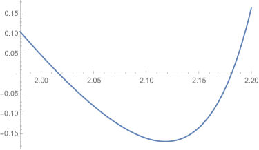
Figure 4. Plot of $R_{-2,m}(2\cos\frac{\pi}{r},y)$ for $m=6$ and $r=14$.

When $y=y_{0}$ we have $\beta=2+(x^{2}-y_{0}-2)\big{(}S_{m}(\alpha)+(1-y_{0})S_{m-1}(\alpha)\big{)}^{2}=x^{2}-y_{0}$. Since $S_{m-2}(\alpha)=\alpha S_{m-1}(\alpha)-S_{m}(\alpha)$ and $S_{m}(\alpha)=1+(y_{0}-1)S_{m-1}(\alpha)$ we get

$$R_{-2,m}(2\cos\frac{\pi}{r},y_{0}) = ((x^{2}-y_{0}-1)S_{m}(\alpha)-S_{m-1}(\alpha))S_{-2}(\beta)$$

$$\qquad\qquad-\,((x^{2}-y_{0}-1)S_{m-1}(\alpha)-S_{m-2}(\alpha))S_{-3}(\beta)$$

$$= -((\beta-1)S_{m}(\alpha)-S_{m-1}(\alpha))+\beta((\beta-1)S_{m-1}(\alpha)-S_{m-2}(\alpha))$$

$$= (\beta^{2}-\beta+1-\beta\alpha)S_{m-1}(\alpha)+S_{m}(\alpha)$$

$$= (\beta^{2}-\beta+1-\beta\alpha+y_{0}-1)S_{m-1}(\alpha)+1.$$

With $\alpha=2+(y_{0}-2)(y_{0}+2-x^{2})=2+(y_{0}-2)(2-\beta)$, by a direct calculation we have $\beta^{2}-\beta+1-\beta\alpha+y_{0}-1=-(\beta-1)(\beta+y_{0}-\beta y_{0})$.

By Lemma 4.7 we have $P(y_{0})=(y_{0}^{2}-y_{0}x^{2}+x^{2})S_{m-1}(\alpha)+y_{0}-x^{2}=0$, which implies that $S_{m-1}(\alpha)=\frac{x^{2}-y_{0}}{y_{0}^{2}-y_{0}x^{2}+x^{2}}=\frac{\beta}{\beta+y_{0}-\beta y_{0}}.$ Hence

$$R_{-2,m}(2\cos\frac{\pi}{r},y_{0})=-(\beta-1)(\beta+y_{0}-\beta y_{0})\frac{\beta}{\beta+y_{0}-\beta y_{0}}+1=1+\beta-\beta^{2}.$$

Hence $R_{-2,m}(2\cos\frac{\pi}{r},y_{0})<0$ if we can show that $\beta>\frac{1+\sqrt{5}}{2}$, i.e. $y_{0}<x^{2}-\frac{1+\sqrt{5}}{2}$.

Let $z:=x^{2}-2=2\cos\frac{2\pi}{r}\geq\frac{3+\sqrt{1-4/m}}{2}$. Then $x^{2}-\frac{1+\sqrt{5}}{2}=z+\frac{3-\sqrt{5}}{2}\geq\frac{3+\sqrt{1-4/m}}{2}+\frac{3-\sqrt{5}}{2}>2$ for $m\geq 6$. Since $P$ is an increasing function on $(2,\infty)$ with a unique root $y_{0}>2$, we conclude that $y_{0}<x^{2}-\frac{1+\sqrt{5}}{2}=z+\frac{3-\sqrt{5}}{2}$ is equivalent to $P(z+\frac{3-\sqrt{5}}{2})>0$.

At $y=y_{1}:=z+\frac{3-\sqrt{5}}{2}$ we have $y^{2}-yx^{2}+x^{2}=\frac{\sqrt{5}-1}{2}(\sqrt{5}-z)$ and $\alpha=\frac{5-\sqrt{5}+(3-\sqrt{5})z}{2}$. This implies that $P(y_{1})=\frac{\sqrt{5}-1}{2}(\sqrt{5}-z)S_{m-1}(\alpha)-\frac{1+\sqrt{5}}{2}$.

If $m\geq 7$ then $z\geq\frac{3+\sqrt{1-4/m}}{2}\geq\frac{3+\sqrt{3/7}}{2}>1.827$ and so $\alpha=\frac{5-\sqrt{5}+(3-\sqrt{5})z}{2}>2.0798$. This implies that $S_{m-1}(\alpha)>S_{6}(2.0798)>12$. Hence

$$P(y_{1})>\frac{\sqrt{5}-1}{2}(\sqrt{5}-2)(12)-\frac{1+\sqrt{5}}{2}=\frac{83-37\sqrt{5}}{2}>0.$$

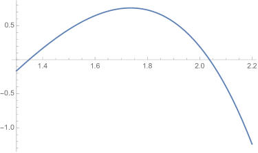
Figure 5. Plot of $P(y)=0$ for $m=6$.

If $m=6$ then $z\geq\frac{3+\sqrt{1-4/m}}{2}\geq\frac{3+\sqrt{2/3}}{2}>1.788$. Since $P(y_{1})=\frac{\sqrt{5}-1}{2}(\sqrt{5}-z)S_{5}(\alpha)-\frac{1+\sqrt{5}}{2}$ where $\alpha=\frac{5-\sqrt{5}+(3-\sqrt{5})z}{2}$, $P(y_{1})$ is a polynomial in $z$ of degree 6 with negative leading coefficient. This polynomial has exactly 6 real roots and the two largest ones are approximately $1.34811$ and $2.03784$ (see Figure 5). Since $z$ lies in the interval between these two roots, we conclude that $P(y_{1})>0$. ∎

Remark 4.9.

In the case $n=-2$ and $m=5$, the bounds $8\leq r\leq 26$ can be checked directly by Mathematica. By numerical experiments, $R_{-2,m}(2\cos\frac{\pi}{r},y)$ does not have any real root $y>2$ if $m=5$ and $r\geq 27$, or $1\leq m\leq 4$ and $r\geq 1$.

4.1.5. Conclusion

We combine the results from all cases to get the following:

Proposition 4.10.

$R_{n,m}(2\cos\frac{\pi}{r},y)=0$ has at least one real solution $y>2$ if:

1. $r\geq 3$ when $n\geq 3$ or $n\leq-4$.

2. $r\geq 4$ when $n=2$ or $n=-3$.

3. $r\geq 5$ when $n=1$ and $m=1,2$, or $n=-2$ and $m=-1$.

4. $r\geq 6$ when $n=1$ and $m\geq 3$, or $n=-2$ and $m\leq-2$.

5. $r\geq 7$ when $n=1$ and $m\leq-4$, or $n=-2$ and $m\geq 6$.

6. $r\geq 8$ when $n=1$ and $m=-2,-3$.

7. $r\geq 9$ when $n=1$ and $m=-1$.

4.2. Proof of Theorem 1

Let $X^{(r)}_{K}$ denote the $r$-th cyclic branched cover of a knot $K$ in $S^{3}$. We will apply the following theorem.

Theorem 4.11 ([BGW, Hu]).

Given any prime knot $K$ in $S^{3}$, denote by $\mu$ a meridional element of the knot group $G(K)$. If there exists a nonabelian representation $\rho:G(K)\to\mathrm{SL}_{2}(\mathbb{R})$ such that $\rho(\mu^{r})=\pm I$, then the fundamental group $\pi_{1}(X^{(r)}_{K})$ is left orderable.

We are now ready to prove Theorem 1. We will prove the case when $n\geq 3$ or $n\leq-4$. The other cases are proved similarly.

Suppose $r\in\mathbb{N}$ satisfies $r\geq 3$ and let $x=2\cos\frac{\pi}{r}$. By Proposition 4.10 there exists $y\in\mathbb{R}$ with $y>2$ such that $R_{n,m}(x,y)=0$. Therefore, we have a nonabelian representation $\rho:G(K_{n,m})\to\mathrm{SL}_{2}(\mathbb{C})$ of the form

$$\rho(a)=\begin{bmatrix}e^{i(\pi/r)}&1\\ 0&e^{-i(\pi/r)}\end{bmatrix},\qquad\rho(b)=\begin{bmatrix}e^{i(\pi/r)}&0\\ -u&e^{-i(\pi/r)}\end{bmatrix}.$$

Note that $x=\text{tr}\rho(a)=2\cos\frac{\pi}{r}$.

Since $y=\text{tr}\rho(ab^{-1})=2+u>2$, we have $u>0$. By [Kh, page 786], the representation $\rho$ can be conjugated to an $\mathrm{SL}_{2}(\mathbb{R})$ representation, denoted by $\rho^{\prime}$. Note that $\rho^{\prime}(a^{r})=-I$ since $\rho(a^{r})=-I$. Therefore, by Theorem 4.11, $\pi_{1}(X^{(r)}_{K_{n,m}})$ is left-orderable.

References

- [1]
- [BGW] S. Boyer, C. Gordon and L. Watson, On L-spaces and left-orderable fundamental groups, Math. Ann., 356 (2013), 1213-1245.
- [DPT] M. Dabkowski, J. Przytycki and A. Togha, Non-left-orderable 3-manifold groups, Canad. Math. Bull., 48 (2005), 32–40.
- [Go] C. Gordon, Riley’s conjecture on representations of 2-bridge knots, J. Knot Theory Ramifications, 26 (2017), 1740003.
- [Hu] Y. Hu, The left-orderability and cycle branched coverings, Algebr. Geom. Topol., 15 (2015), 399-413.
- [Kh] V. Khoi, A cut-and-paste method for computing the Seifert volumes, Math. Ann., 326 (2003), 759-801.
- [OS] P. Ozsváth and Z. Szabó On knot Floer homology and lens space surgeries, Topology, 44 (2005), 1281–1300.
- [Ri] R. Riley, Nonabelian representations of 2-bridge knot groups, Quart. J. Math. Oxford Ser. (2), 35 (1984), 191–208.
- [Tr1] A. Tran, Nonabelian representations and signatures of double twist knots, J. Knot Theory Ramifications 25 (2016), 1640013, 9 pp.
- [Tr2] A. Tran, On left-orderability and cyclic branched coverings, J. Math. Soc. Japan 67 (2015), no. 3, 1169–1178.
- [Tr3] A. Tran, Reidemeister torsion and Dehn surgery on twist knots, Tokyo J. Math., 39 (2016), 517–526.
- [Tu] H. Turner, Left-oderability, branched covers and double twist knots, preprint, arXiv:2002.10611.