The Field Substellar Mass Function Based on the Full-sky 20-pc Census of 525 L, T, and Y Dwarfs

Abstract

We present final Spitzer trigonometric parallaxes for 361 L, T, and Y dwarfs. We combine these with prior studies to build a list of 525 known L, T, and Y dwarfs within 20 pc of the Sun, 38 of which are presented here for the first time. Using published photometry and spectroscopy as well as our own follow-up, we present an array of color-magnitude and color-color diagrams to further characterize census members, and we provide polynomial fits to the bulk trends. Using these characterizations, we assign each object a $T_{\rm eff}$ value and judge sample completeness over bins of $T_{\rm eff}$ and spectral type. Except for types $\geq$ T8 and $T_{\rm eff}<$ 600K, our census is statistically complete to the 20-pc limit. We compare our measured space densities to simulated density distributions and find that the best fit is a power law ($dN/dM\propto M^{-\alpha}$) with $\alpha=0.6{\pm}0.1$. We find that the evolutionary models of Saumon & Marley correctly predict the observed magnitude of the space density spike seen at 1200K $<T_{\rm eff}<$ 1350K, believed to be caused by an increase in the cooling timescale across the L/T transition. Defining the low-mass terminus using this sample requires a more statistically robust and complete sample of dwarfs $\geq$Y0.5 and with $T_{\rm eff}<$ 400K. We conclude that such frigid objects must exist in substantial numbers, despite the fact that few have so far been identified, and we discuss possible reasons why they have largely eluded detection.

1 Introduction

We now find ourselves at a moment in history where selecting parallax-based censuses of nearby objects from the hottest O stars to the coldest Y dwarfs is almost a reality. With the release of Gaia Data Release 2 (DR2; Gaia Collaboration et al. 2018) and Data Release 3 (scheduled for the first half of 2022), the astronomical community can begin extracting complete, volume-limited samples out to distances which provide exquisite statistics on the distribution of stellar types. As a result of operating at wavelengths $<$1 $\mu$m and selecting a conservative detection threshold, Gaia provides complete astrometry only for L5 dwarfs out to $\sim$24 pc (Smart et al. 2017). Extending this census to colder types, though, is more easily accomplished by ground-based or space-based astrometric monitoring at longer wavelengths, where late-L, T, and Y dwarfs are brightest. A complete, volume-limited census across all stellar and substellar types is extremely useful in a variety of investigations, including: (1) analysis of the mass function, (2) determining the frequency of binaries across all types, (3) providing a catalog of host stars around which the nearest habitable planets to our own Solar System can be searched, and (4) establishing correlations among colors, absolute magnitudes, spectral types, effective temperatures, etc. that can be applied to other samples whose parallaxes are unknown or not so easily measured.

In this paper we provide the cold dwarf complement to the complete, nearby samples being extracted from Gaia. Our contribution is twofold. One, we present analysis on a flurry of new discovereies by the Backyard Worlds: Planet 9 (hereafter, "Backyard Worlds") and CatWISE teams that in the last several months have helped to identify even more previously hidden members of the 20-pc census. Two, we present a set of 361 parallaxes measured by the Spitzer Space Telescope (hereafter, Spitzer) that, when combined with astrometric monitoring of other objects by the astronomical community, establishes a complete, full-sky, volume-limited census of L, T and Y dwarfs out to 20 pc. We use this census to establish the shape and functional form of the mass function in the substellar regime.

This paper is organized as follows. In section 2 we provide motivation for studying the mass function and describe what can be learned from the results. In section 3 we build the seed list of targets for the 20-pc L, T, and Y census and describe how this parallels historical efforts to catalog nearby stars of types M and earlier. In section 4 we discuss our Spitzer data acquisition and the subsequent astrometric reductions, and we compare our results to other published parallaxes for objects with independent measurements. In section 5 we discuss photometric and spectroscopic follow-up in support of the 20-pc seed list. In section 6 we construct the final 20-pc census, and in section 7 we examine outliers on various color-color and color-magnitude diagrams in order to more carefully characterize objects in the census. In section 8 we assign values of $T_{\rm eff}$ to each object, then calculate space densities as a function of $T_{\rm eff}$, once we have determined completeness limits and completeness corrections. In section 9 we provide the best fits of these measured space densities to predictions. These predictions simulate space densities for various forms of the mass function passed through two different sets of evolutionary models. We also discuss the value of the low-mass cutoff and ponder why so few brown dwarfs with $T_{\rm eff}<$ 400K have been uncovered to date. We conclude with future avenues of exploration in section 10.

2 Why Explore the Mass Function?

What does an analysis of the mass function tell us? The astronomical literature is replete with arguments about the functional form of the overall mass function, but what knowledge do we gain from its determination?

The two main, competing forms for the stellar mass function are the power law and the log-normal. At a fundamental level, a power law would inform us that the physical process is scale-free, meaning that the mass of the natal cloud has no bearing on the final stellar mass distribution, only on the total number of objects formed. That is, the relative distribution of masses formed from a small cloud will be the same as that from a much more massive cloud. A power law functional form would therefore imply a single physical process reigning over all of star production. If a universal power law is the correct form, then averaging results over many different star formation sites – as we do when looking at an older, well mixed, volume-limited sample near the Sun – should still result in a mass distribution with a power law form.

Even if a power law form describes the observed data, it is common in Nature to find that it applies only above some minimum value. For example, in investigations such as the peak intensity of solar flares or the magnitudes of earthquakes, a power law fits the data well only if a minimum value is imposed (Clauset et al. 2009). To employ a reductio ad absurdum of our own, there must be a minimum value for the cut-off mass of star formation because Nature cannot create a star containing only one atom.

The log-normal form, on the other hand, is the result expected when there are many processes that contribute multiplicatively to the result. (Contrast this to a normal distribution, which is the result of processes that contribute additively.) As Kapteyn (1903) elegantly argued, even if some physical processes, like the swelling in diameter of a growing blueberry (or a stellar embryo), appear to be normally distributed – i.e., a symmetric distribution centered on some mean value – other quantities, such as the growing volumes of those blueberries (or stars), would necessarily have skewed distributions. He argued that skewed forms are, in fact, favored over symmetrical ones. Many of Nature’s skewed distributions are well characterized by a log-normal form (Limpert et al. 2001), again implying that several independent processes are working together to produce the final outcome (Miller & Scalo 1979).

If a single functional form fails to describe the observed distribution over the entire mass range from O stars to Y dwarfs – and it is well known that there is a break in the shape of the mass function below 1 M_⊙ (see Figure 2 of Bastian et al. 2010, who give an overview of the stellar initial mass function) – then the inflection in the shape of the mass function roughly corresponds to the mass at which a new set of physical processes is becoming dominant. In fact, the mass function may have several inflection points, indicating that separate sets dominate in different mass regimes.

Even with solid knowledge of the mass function’s shape across the entire mass spectrum of interest – in our case, over the entirety of the brown dwarf masses – divining the physical causes responsible for that shape will be difficult. Nonetheless, knowing the shape enables a semi-empirical determination of the low-mass cutoff and allows us to build simulations that better reflect true space densities across all spectral types.

3 Building the Target List

Since the 1988 discovery of GD 165B (Becklin & Zuckerman 1988), large swaths of the astronomical community have contributed to uncovering hidden L, T and Y dwarfs in the immediate solar vicinity. New members of the 20-pc census have been announced not only by brown dwarf researchers specifically looking for examples (e.g., Kendall, et al. 2004), but also by researchers in unassociated fields who have serendipitously found others (e.g., Hall 2002, Thorstensen & Kirkpatrick 2003). New additions to the sample have been published as single-object papers (e.g., Ruiz et al. 1997, Folkes, et al. 2007); as part of large photometric (e.g., Delfosse et al. 1997, Lucas et al. 2010), spectroscopic (e.g., Schmidt, et al. 2010), proper motion (e.g., Smith et al. 2014, Meisner et al. 2020a, b), or parallax surveys (e.g., from Gaia: Reylé 2018, Scholz 2020); or as the result of dedicated searches for companions around higher mass stars (e.g., Thalmann et al. 2009, Freed et al. 2003) or around other brown dwarfs (e.g., Volk et al. 2003, Gelino et al. 2011). Construction of the census of the closest L, T, and Y dwarfs has been the effort of many dozens of lead authors presenting results in hundreds of publications.

3.1 A Nearby Census in its Historical Context

Compiling these results into a volume-limited data set is a difficult task. To place this in historical context, consider that the first parallax – that of the 3.5-pc distant 61 Cygni AB – was obtained in 1838 by Bessel (1838). Few stars were bright enough and near enough to the Sun to have accurate astrometry measured, but there was enough information seven decades later for Hertzsprung (1907) to compile what may have been the first list of nearby stars (see Batten 1998). It was not until 1913-1914 that the first M dwarfs with both a parallax and a measured spectral type were published – Groombridge 34 (Adams 1913) and Lalande 21185 (Adams & Kohlschütter 1914). This prompted Hertzsprung (1922) to update his previous paper, the new list having just under thirty stars confirmed to lie within 5 pc of the Sun. Just four years later, nearly a hundred nearby M dwarfs had been identified (Adams et al. 1926). Occasional updates on the 5.2-pc sample were made for years thereafter by van de Kamp (1930, 1940, 1945, 1953, 1955, 1969, 1971), the last update containing a total of sixty stars, including the Sun. Kuiper (1942) published a larger list, pushing out to 10.5 pc, that contained 254 individual objects. In more recent times, similar lists have appeared, such as the online list of the top one hundred closest systems – which as of the last update in 2012 extends to a radius of 6.95 pc from the Sun – by the Research Consortium On Nearby Stars (RECONS) team, or the 8-pc census presented by Kirkpatrick et al. (2012) that contained 243 individual objects.

The above lists, however, have inadequate statistics with which to perform any meaningful analysis of the mass function. Other lists, covering a more substantial volume, are clearly needed for this work, and such compilations were amassed in the latter half of the twentieth century. The 20-pc catalog of Gliese (1957) contained 1,097 individual objects, and a second catalog was produced over a decade later (Gliese 1969) to update that number to 1,890. A supplement to the second catalog was published by Gliese & Jahreiß (1979) and listed an additional 462 objects. A third catalog, produced on CD-ROM (Gliese & Jahreiß 1991) but never published in a refereed journal, contained over 3,800 entries within 25 pc. A fourth catalog, promised around 1999, never materialized. These catalogs have now been superseded by Gaia.

The list of nearby L, T, and Y dwarfs, on the other hand, has not been superseded, because Gaia can acquire accurate astrometry for L5 dwarfs out to only $\sim$24 pc, T0 dwarfs to only $\sim$12 pc, T5 dwarfs to only $\sim$10 pc, and T9 dwarfs to only $\sim$2 pc (Smart et al. 2017). As argued in Kirkpatrick et al. (2019), a 20-pc census provides adequate statistics for determining the mass function in the L, T, and Y dwarf regime, and 20 pc is also the maximum distance at which a census of Y0 dwarfs can be constructed, given the sensitivity limits of Wide-field Infrared Survey Explorer (WISE; Wright et al. 2010) data. Best et al. (2020) have argued for a partial-sky 25-pc census for low-mass mass function studies; however, their desire to perform astrometric follow-up from the United Kingdom Infrared Telescope (UKIRT) restricts them to $-30^{\circ}<\delta<+60^{\circ}$, so their increase in volume over a full-sky 20-pc census is only $\sim$33%.

In order to construct a census of nearby, low-mass dwarfs, we began constructing an archive in 2003 (Kirkpatrick 2003) to amass published discoveries of all L and T dwarfs along with their near-infrared photometry and spectral types. At the time the catalog was begun, the list of L and T dwarfs contained 277 objects. Shortly thereafter, the list had grown into a publicly available online database listing 470 L and T dwarfs (Gelino et al. 2004). By 2009 this number had grown to over 650 L and T dwarfs (Gelino et al. 2009), and by late 2012, which was the last online update, the list had grown to 1,281 L, T, and Y dwarfs. Other researchers provided their own post-2012 updates; the Mace (2014) list had 1,565 entries and the List of UltraCool Dwarfs had 1,773, although neither of those has been updated in the last 5+ years. One of us (CRG) maintains an in-house spreadsheet that captures new discoveries from the literature, and at its last update in Oct 2019, it contained 2,513 L, T and Y dwarfs.

3.2 Building a List of Probable 20-pc L, T, and Y Dwarfs

The efforts above provided the cornerstones for the building of a volume-limited census needed for this paper. For each of the known L, T, and Y dwarfs, the object’s spectral type and magnitudes in the WISE W2 band and in $H$ band, the latter of which is invariant between the 2MASS and MKO filter systems (see Kirkpatrick et al. 2019), were tabulated. Using the color/spectral type to absolute magnitude relations presented in Kirkpatrick et al. (2012) and Looper et al. (2008a), we calculated spectrophotometric distance estimates and retained all objects having d $<$ 23 pc. Separately, we combed the literature in search of published trigonometric parallaxes for each of the known L, T, and Y dwarfs, many of which were already compiled in the CRG spreadsheet noted above. Objects with trigonometric parallaxes measured to better than 10% accuracy and falling within 20 pc were kept in our official nearby census, and those lacking a parallax with 10% accuracy or lacking astrometric follow-up entirely but having distance estimates within 23 pc were retained for further astrometric monitoring with Spitzer. This limit was chosen to account for margin of error in the distance estimates, the expectation being that most objects truly within 20 pc would have estimates placing them within 23 pc.

In Kirkpatrick et al. (2019), we used the Infrared Array Camera (IRAC; Fazio et al. 2004) to measure preliminary trigonometric parallaxes for those objects having spectral types of T6 and later. These results were based on data from Spitzer programs 70062, 80109, 90007, 11059, and the first year’s data from 13012 (all with Kirkpatrick as PI). This left a gap in the L and T dwarf sequence between T6 and the latest type for which Gaia has complete coverage ($\sim$L5). The aim of Spitzer program 14000 (Kirkpatrick, PI) was to astrometrically monitor those objects in the gap that lacked published parallaxes of high quality but were believed to fall within 23 pc. An extension to provide additional data points for these objects at the end of the Spitzer mission was further approved as program 14326 (Kirkpatrick, PI).

Meanwhile, old WISE data and newer Near Earth Object WISE (NEOWISE; Mainzer et al. 2014) data were being continually processed, searched, re-processed, and re-searched in hopes of uncovering new objects at the coldest types, since Kirkpatrick et al. (2019) found that the targets in that paper were not complete to 20 pc for any of the late-T or Y dwarf types. Specifically, their measured completeness limits ranged from 19 pc at T6 to only 8 pc at Y0. Both the Backyard Worlds (Kuchner et al. 2017) and CatWISE (Eisenhardt et al. 2020) teams were continuing to identify new candidate late-T and Y dwarfs from WISE data as Spitzer hurled toward its assigned decommissioning date in late-Jan 2020. As chronicled in Meisner et al. (2020a, b), candidates lacking extant Spitzer photometry were added to Spitzer photometric programs 14034 (Meisner, PI), 14076 (Faherty, PI), and 14299 (Faherty, PI). As these new IRAC data became available, we used the new Spitzer photometry to predict a distance to each candidate using the $M_{\rm ch2}$ vs. ch1$-$ch2 color relation of Kirkpatrick et al. (2019). Such objects with spectrophotometric distance estimates $<$23 pc were the subject of yet another Spitzer astrometric follow-up program (14224; Kirkpatrick, PI).

Not all of the late-type candidates were included in programs 14034, 14076, or 14299, however, either because ch1$-$ch2 data already existed in the Spitzer Heritage Archive, mainly from our own, earlier programs (70062, 80109, or 11059), or because their discoveries occurred after the end of the Spitzer mission. These objects, which were selected by the community scientists of Backyard Worlds, team members of CatWISE, or both were uncovered via the same selection criteria discussed in Meisner et al. (2020a, b) and are listed in Table 1. Also included in this table are additional late-T and Y dwarf candidates, observed as part of Spitzer photometric program 14329 (Marocco, PI), that were discovered as part of the CatWISE2020 effort (Marocco et al. 2020b) and have not previously been published.

Table 1: New L, T, and Y Dwarf Candidates

Object	Note	Discoverer Code
(1)	(2)	(3)
CWISE J002727.44$-$012101.7	astrom	C, F, J, N, Q, R, S, W
CWISE J004143.77$-$401929.9	astrom	C, D, F, G, H, J, K, Q, R
CWISE J004311.24$-$382225.0	astrom	F, G, J, K, R, V
CWISE J011558.74$-$461620.8	—	A, F, G, J, K, Q
CWISE J011931.78$-$493750.4	—	F, G, J, K, W
CWISE J011952.82$-$450231.2	—	A, D, K, N
CWISE J014308.73$-$703359.1	—	B, F, G, J, K, Q
CWISE J014837.51$-$104805.6	astrom	F, G, K, N
CWISE J015042.24$-$462155.3	—	F, G, I, J, K, N, Q
CWISE J015349.89+613746.3	new	V
CWISE J021705.51+075849.9	new	A, D
CWISE J031021.61$-$573355.6	—	C, G, J, K, M, Q
CWISE J034146.12+471530.5	new	G, V
CWISE J041102.41+471422.6	new	A, D, N, R, W
CWISE J042335.38$-$401929.5	astrom	J
CWISE J044214.20$-$385515.7	astrom	J
CWISE J051427.35+200447.7	new	D, G, S
CWISE J054025.89$-$180240.3	astrom	C
CWISE J060149.45+141955.2	new	G
CWISE J060251.35$-$403534.4	—	C, J, K
CWISE J061348.70+480820.5	astrom	A, G
CWISE J061741.79+194512.8	new	G, Z
CWISE J062050.79$-$300620.8	new	C, G, V
CWISE J062725.28$-$373033.1	—	A, C, G
CWISE J063018.23$-$371734.3	—	A, G, J, N, Q
CWISE J063031.50$-$600221.0	—	A, C, G, J, K
CWISE J063558.52$-$322549.4	color	D, F, S, V
CWISE J063649.77$-$542429.2	new	G, V
CWISE J064128.15$-$312359.3	—	J, K, Q
CWISE J064223.54+042342.2	astrom	D, Z
CWISE J064749.87$-$160022.7	—	D, G, P, N
CWISE J074956.20$-$682722.4	—	B, F, G, J, K
CWISE J075648.34$-$600130.9	—	A, G, J, K
CWISE J075831.11+571153.9	—	F, G, J, K, N, Q, S, X, Z
CWISE J080436.67$-$000028.6	—	A, D
CWISE J080556.14+515330.4	—	D, G, L, S, V
CWISE J081606.70+482822.9	—	B, D, S
CWISE J084506.51$-$330532.7	new	G, D, S
CWISE J085401.22$-$502028.1	—	A, E, F, G, J, K
CWISE J091105.02+214645.1	astrom	C, D, F, J, K, S, T
CWISE J091735.38$-$634451.2	new	A
CWISE J092503.20$-$472013.8	new	L, S
CWISE J093823.15$-$841114.4	color	D, F, L, S
CWISE J094925.88$-$102601.9	—	A, D, F, J, N, Q
CWISE J095316.32$-$094318.9	—	A, F, J, K, Q
CWISE J105512.11+544328.3	astrom	D, G, J
CWISE J110201.76+350334.7	new	A, J, N, S, V
CWISE J112106.36$-$623221.5	new	L, S
CWISE J113019.19$-$115811.3	astrom	B, D, F, J, K
CWISE J113717.27$-$532007.9	astrom	A, F, G, J, K
CWISE J113833.47+721207.8	astrom	F, G, J, K, Q
CWISE J114120.42$-$211024.5	astrom	A, C, F, G, J, S, V
CWISE J115229.37$-$374157.8	—	A, D, G, J
CWISE J120502.74$-$180215.5	astrom	D, G, J, K, Y
CWISE J121557.87+270154.2	—	F, G, J, K, Q, S
CWISE J123228.86+225714.5	—	C, D, N, Z
CWISE J130841.31$-$032157.7	new	G, L, V
CWISE J131548.23$-$493645.4	new	C, S
CWISE J141127.70$-$481153.4	astrom	A, J
CWISE J153143.38-330657.3	new	G, S, V
CWISE J153347.50+175306.7	astrom	G, J, K, N
CWISE J163041.79$-$064338.3	new	A, D, G, U
CWISE J165013.37+565257.0	new	A, G, S, V
CWISE J170127.12+415805.3	astrom	C, D, F, G, J, N, P, Q, V, Z
CWISE J172617.09$-$484424.9	new	A, E
CWISE J174907.16+554050.3	color	A, F, Z
CWISE J175517.35+250147.3	—	F, G, J, K, L, N, Q
CWISE J175628.97+505328.5	color	F
CWISE J175800.46+555322.7	color	F, S
CWISE J182755.05+564507.8	new	G, Q
CWISE J183207.94$-$540943.3	astrom	C, Y
CWISE J185104.34$-$245232.1	new	G, S
CWISE J192537.88+290159.0	color	E, F, S
CWISE J192636.29$-$342955.7	astrom	A, B, K, J, M, Q
CWISE J193823.28+663602.7	—	J, S, Z
CWISE J193824.10+350025.0	color	F, L, S
CWISE J194201.42+534830.5	color	F, L, S
CWISE J195228.45$-$730049.4	new	B, D, G, Q
CWISE J200121.21$-$413606.8	—	A, B, C, F, J, Q, T
CWISE J201221.32+701740.2	astrom	D, J, L
CWISE J201342.27$-$032643.7	new	B, F, G, J, K
CWISE J203859.15$-$570110.3	color	F
CWISE J205701.64$-$170407.3	astrom	J, N, S, V
CWISE J234426.81$-$475502.6	—	G
CWISE J235448.04$-$814044.6	—	G, J, K, N

Note. — Reference code for discoverer: A = Andersen, B = Beaulieu, C = Colin, D = Caselden, E = Stenner, F = Marocco, G = Goodman, H = Hamlet, I = Voloshin, J = Kirkpatrick, K = Khalil, L = Gramaize, M = D. Martin, N = Ammar, P = Pendrill, Q = Hong, R = Rothermich, S = Sainio, T = Tanner, U = Hinckley, V = Thévenot, W = Walla, X = Jonkeren, Y = Pumphrey, Z = Wędracki.

Note. — Discoveries in this table were scrutinized using the online WiseView tool (Caselden et al. 2018).

Sometime after Spitzer program 14224 was selected for 246.5 hours of data collection, we were informed that, for unforeseen logistical reasons at the Spitzer Science Center, the originally planned 2019 Apr 15 start date of our observations would have to be moved to 2019 Jun 16 and that our allotted time would be halved. This had two ramifications for the intended science: (1) In order to get enough astrometric data points for a meaningful parallactic solution, we had to remove many of the original targets in the program, and (2) the later start date meant that we would only be able to obtain observations at one additional epoch for those targets with a visibility window that closed between Apr 15 and Jun 16, which was roughly one-third of the targets. As a result, we dropped most of the objects in our program with spectrophotometric distance estimates between 20 and 23 pc, along with some of those with the earliest types (around T6). We were also forced to rely more heavily on outside astrometry since our Spitzer data would now cover an insufficient time baseline to disentangle the effects of parallax and proper motion. More discussion of this can be found in section 4.

Table 2 lists all 361 targets that were eventually observed in one of our Spitzer parallax programs. In total, 98.7% of the Astronomical Observation Requests (AORs) in the table were from programs proposed by various WISE, CatWISE, and Backyard Worlds team members. We used the Spitzer Heritage Archive to supplement our 5,041 AORs with another 66 from other researchers, which primarily enabled us to extend the time baseline of the Spitzer data set. Table 3 lists the individual Spitzer programs whose data were used. Of these 66 supplementary observations, fifteen were taken during the original Spitzer cryogenic mission and were reduced using software applicable to that mission phase, as described in more detail in section 4.

Table 2: Objects on the IRAC ch2 Spitzer Parallax Programs

Object	First Obs. Date	Last Obs. Date	Baseline	Program # (and # of Epochs)
Name	(UT)	(UT)	(yr)	with ch2 Coverage
(1)	(2)	(3)	(4)	(5)
WISE 0005+3737	2012 Sep 06	2018 May 02	5.7	80109(1), 90007(12), 13012(12)
WISE 0015$-$4615	2010 Dec 17	2018 Oct 04	7.8	70062(2), 90007(12), 13012(12)
CWISE 0027$-$0121	2015 Feb 25	2019 Nov 26	4.8	10135(1), 11059(1), 14224(6)
WISE 0031+5749	2018 Nov 18	2020 Jan 15	1.2	14000(9), 14326(2)
PSO 0031+3335	2018 Nov 05	2019 Nov 25	1.1	14000(9)
WISE 0032$-$4946	2012 Jul 28	2018 Sep 23	6.2	80109(1), 90007(12), 13012(12)
2MASS 0034+0523	2012 Feb 15	2018 Apr 23	6.2	80109(2), 90007(12), 13012(12)
WISE 0038+2758	2012 Mar 22	2018 May 05	6.1	80109(2), 90007(14), 13012(12)

Note. — (This table is available in its entirety in a machine-readable form in the online journal. A portion is shown here for guidance regarding its form and content.)

Table 3: Spitzer Programs with ch2 Data Used in the Astrometric Analysis

Program	Type	# of ch2	Principal
#		AORs	Investigator
(1)	(2)	(3)	(4)
35*	GTO	1	Fazio
244*	DDT	1	Metchev
3136*	GO	2	Cruz
20514*	GO	3	Golimowski
30298*	GO	3	Luhman
40198*	GTO	4	Fazio
50059*	GO	1	Burgasser
60046	GO	10	Luhman
60093	GO	1	Leggett
551	DDT	1	Mainzer
70021	SNAP	4	Luhman
70058	GO	1	Leggett
70062	GO	175	Kirkpatrick
80077	GO	2	Leggett
80109	GO	212	Kirkpatrick
90007	GO	870	Kirkpatrick
90095	GO	4	Luhman
10135	GO	3	Pinfield
10168	DDT	4	Luhman
11059	GO	9	Kirkpatrick
13012	GO	1704	Kirkpatrick
14000	GO	1404	Kirkpatrick
14034	GO	33	Meisner
14076	GO	18	Faherty
14224	DDT	485	Kirkpatrick
14299	DDT	2	Faherty
14326	DDT	131	Kirkpatrick

Note. — An asterisk indicates a program from the Spitzer cryogenic mission (ending 2009 May).

4 Astrometric Data Acquisition and Reduction

The reduction of the Spitzer astrometry used the same methodology as that outlined in section 5.2 of Kirkpatrick et al. (2019), with the following exceptions. First, the list of possible re-registration stars was paired not against Gaia Data Release 1 (DR1) but with the newer Gaia DR2 instead, as the latter contains five-parameter ($\alpha_{0}$, $\delta_{0}$, $\varpi_{abs}$, $\mu_{\alpha}$, and $\mu_{\delta}$) solutions for $\sim$70% of cataloged objects. Second, we used these full astrometric solutions to predict the per-epoch positions of each re-registration star at the observation date of each AOR, thereby enabling us to measure absolute parallaxes and proper motions of the Spitzer targets directly. Third, to assure that we had a sufficient number of five-parameter Gaia DR2 re-registration stars per frame, we set the signal-to-noise (S/N) requirement to S/N $\geq$ 30 per frame; in Kirkpatrick et al. (2019), we used S/N $\geq$ 30 only when the field for that target was starved of S/N $\geq$ 100 background stars. As stated in that paper, however, the inclusion of re-registration stars with 30 $<$ S/N $<$ 100 does not generally degrade the $\chi^{2}$ values of the final parallax and proper motion solution compared to solutions using S/N $\geq$ 100 stars only. Fourth, one small modification to the astrometric solution was included for these new reductions. In Kirkpatrick et al. (2019), the mean epoch for all solutions was set to 2014.0 because the time span for each of the objects was similar. The time coverage of the new data set, however, varies greatly from object to object (see Table 2), so we have chosen to compute and report the mean epoch of each object separately.

For those AORs in Table 3 that came from the cryogenic portion of the Spitzer mission, we modified our reductions slightly. During the single-frame reduction step detailed in section 5.2.2 of Kirkpatrick et al. (2019), we ran the MOPEX/APEX software so that the Point Response Function (PRF) fitting made use of the PRF maps measured for cryogenic data. All data from the warm mission were, as before, reduced using PRF maps applicable to the warm phase.

As stated in section 3.2, some of our Spitzer astrometry from Cycle 14 lacked a sufficient time baseline with which to disentangle proper motion and parallax, so we supplemented the Spitzer data with positions derived from the unWISE (Lang 2014) "time-resolved" coadds of Meisner et al. (2018a, b). The methodology is the same as that described in section 8.3 of Meisner et al. (2020a), which measures the positions of our sources on the time-resolved unWISE coadds whose astrometry has been re-registered to the Gaia DR2 reference frame. The unWISE measurements used here are the NEO5 version of the time-resolved coadds, covering early 2010 through late 2018. For this current work, however, the coadds were produced on an epochal basis; that is, because we needed a clearly defined time stamp, positions were not combined across differing time-resolved sets (usually spaced by six months), as was done in Meisner et al. (2020a) to increase the S/N of the final detection.

Because our planned observations between 2019 Apr 15 and 2019 Jun 16 never materialized (see section 3.2), thirteen of our 361 sources had Spitzer observations sampling only one side of the parallactic ellipse and thus, only a proper motion measurement was possible. For these cases, the same fitting procedure outlined above was used except that the parallax term was set to zero.

For each target, a listing of all of the measured positions from our Spitzer reductions– and from the unWISE reductions, if applicable – is given in Table 4. Per the above discussion, all positions are re-registered to the Gaia DR2 reference frame and have uncertainties and time stamps attached. Additional information regarding registration of the unWISE astrometry can be found in section 8.3 of Meisner et al. (2020a).

Table 4: Astrometry on the Gaia DR2 Reference Frame

Object	RA	Dec	$\sigma_{\rm RA}$	$\sigma_{\rm Dec}$	Source	MJD	$X$	$Y$	$Z$
	(deg)	(deg)	(asec)	(asec)		(day)	(km)	(km)	(km)
(1)	(2)	(3)	(4)	(5)	(6)	(7)	(8)	(9)	(10)
0005+3737	1.323697	37.622181	0.010	0.010	ch2	56176.54	28532439.95	-137033306.05	-61329018.68
0005+3737	1.324420	37.622029	0.010	0.010	ch2	56923.88	30795904.89	-136653138.81	-61123398.32
0005+3737	1.324171	37.622031	0.010	0.010	ch2	56750.45	-57605421.64	127020923.18	56379531.75
0005+3737	1.324158	37.622036	0.010	0.010	ch2	56736.94	-24304166.88	135745713.92	60811831.23
0005+3737	1.324143	37.622043	0.010	0.010	ch2	56724.04	8722950.84	137418753.36	62061969.36
0005+3737	1.324141	37.622048	0.010	0.010	ch2	56714.29	33502880.86	134324880.85	61039865.73

Note. — The column Object includes only the first four digits of the sexagesimal RA and the first four digits (plus the sign) of the sexagesimal Dec.

Note. — References for Source: ch2 = Spitzer ch2 astrometry, W1 = WISE astrometry from the Gaia-registered unWISE time-resolved coadds in W1, W2 = WISE astrometry from the Gaia-registered unWISE time-resolved coadds in W2.

Note. — (This table is available in its entirety in a machine-readable form in the online journal. A portion is shown here for guidance regarding its form and content.)

Because the two sets of astrometry are taken from different positions within our Solar System – one from the Earth-orbiting WISE spacecraft and the other from the Sun-orbiting Spitzer spacecraft – all observations were tagged with the $XYZ$ positions within the Solar System corresponding to the Modified Julian Date (MJD) of the data. For Spitzer observations, these $XYZ$ positions are tabulated by the Spitzer Science Center in the FITS image headers; for the unWISE epochs, we used the mean MJD of each epochal coadd and assigned to them the $XYZ$ of the Earth at that time, using data available through the JPL Horizons website. Note that the use of the Earth’s position is sufficient since the unWISE epochal data themselves are an average over a few days of WISE observations near that mean epoch. Even with the inclusion of non-Spitzer astrometry into the astrometric solutions, no special modifications to the fitting routine employed in section 5.2.3 of Kirkpatrick et al. (2019) were needed. It should be noted that, with the exception of a very small number of confused observations noted in Table 2, all astrometric data points were used in the fits since no sigma clipping and refitting were performed.

In principle, the unWISE epochal astrometry was needed only for those Spitzer data sets that had observations covering fewer than three Spitzer visibility windows. In practice, however, we included unWISE data into the astrometric solutions for all objects in programs 14000, 14224, and 14326; the only exceptions were objects in common to program 13012, as these already had Spitzer observations spanning multiple years.

Plots of our astrometric measurements and their best fits are shown in Figure Set 1 for each of our 361 targets. Figures 1a, 1b, and 1c show examples of the three types of plots found within the figure set.

Fig. Set1. Astrometric fits to the 361 objects in the Spitzer parallax program

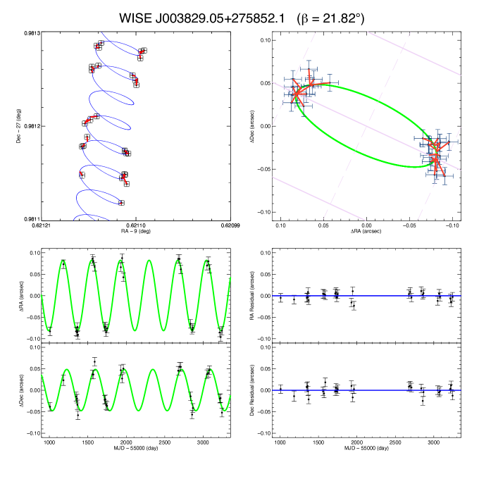
Figure 1a: Example of a target whose astrometric fit uses only Spitzer data. (Upper left) A square patch of sky showing the measured astrometry and its uncertainty at each epoch (black points with error bars) plotted in RA vs. Dec. The blue curve shows the best fit. Red lines connect each observation to its corresponding time point along the best-fit curve. (Upper right) A square patch of sky centered at the mean equatorial position of the target. The green curve is the parallactic fit, which is just the blue curve in the previous panel with the proper motion vector removed. Again, red lines connect the time of the observation with its prediction. In the background is the ecliptic coordinate grid, with lines of constant $\beta$ shown in solid pale purple and lines of constant $\lambda$ shown in dashed pale purple. Grid lines are shown at 0$\farcs$1 spacing. (Lower left) The change in RA and Dec as a function of time with the proper motion component removed. The parallactic fit is again shown in green. (Lower right) The RA and Dec residuals from the fit as a function of time.

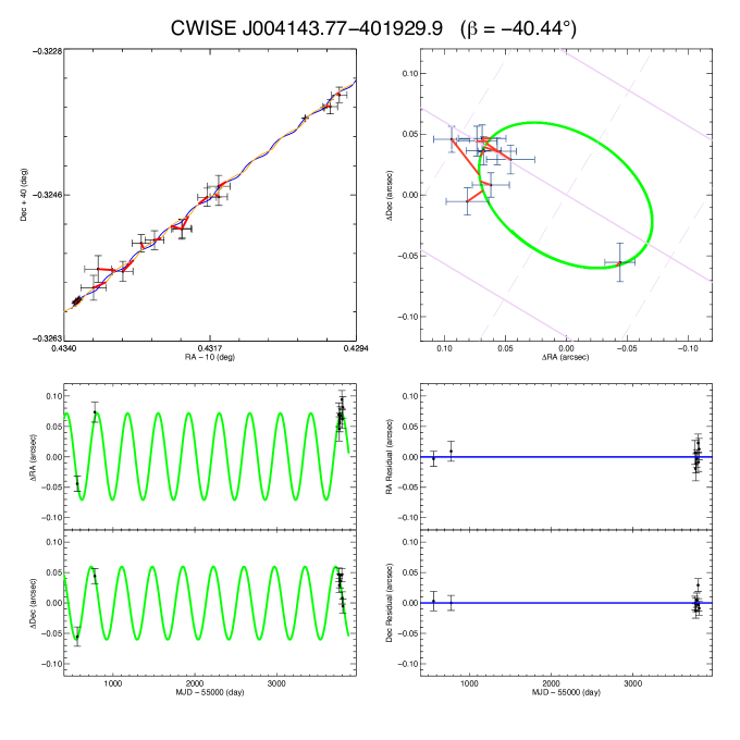
Figure 1b: Example of a target whose astrometric fit uses both Spitzer and unWISE data. (Upper left) A square patch of sky showing the measured astrometry and its uncertainty at each epoch (black points with error bars) plotted in RA vs. Dec. Points with small error bars are the Spitzer ch2 measurements; those with larger error bars are the WISE W1 and W2 measurements. The blue curve shows the best fit from the vantage point of Spitzer, and the orange curve shows this same fit as seen from the vantage point of WISE. Red lines connect each observation to its corresponding time point along the best-fit curve. (Upper right) A square patch of sky centered at the mean equatorial position of the target. The green curve is the parallactic fit, which is just the blue curve in the previous panel with the proper motion vector removed. For clarity, only the Spitzer astrometric points are shown, again with red lines connecting the time of the observation with its prediction. In the background is the ecliptic coordinate grid, with lines of constant $\beta$ shown in solid pale purple and lines of constant $\lambda$ shown in dashed pale purple. Grid lines are shown at 0$\farcs$1 spacing. (Lower left) The change in RA and Dec as a function of time with the proper motion component removed. The parallactic fit is again shown in green and only the Spitzer astrometry is shown. (Lower right) The RA and Dec residuals from the fit as a function of time. As with the lower left panel, only the Spitzer data are shown.

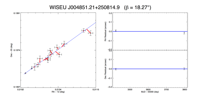
Figure 1c: Example of a target whose astrometric fit uses both Spitzer and unWISE data but for which a parallactic fit could not be attempted. (Left) A square patch of sky showing the measured astrometry and its uncertainty at each epoch (black points with error bars) plotted in RA vs. Dec. Points with small error bars are the Spitzer ch2 measurements; those with larger error bars are the WISE W1 and W2 measurements. The blue curve shows the best proper motion fit. Red lines connect each observation to its corresponding time point along the best-fit curve. (Right) The RA and Dec residuals from the fit as a function of time. Only the Spitzer data are shown since the error bars of the WISE points would otherwise dominate the plot.

Our astrometric results are summarized in Tables 5, 6, and 7. For each object, the RA and Dec position (in deg) with their uncertainties (in mas) are quoted at the mean epoch, $t_{0}$, along with the absolute parallax ($\varpi_{abs}$) and absolute proper motions ($\mu_{RA}$ and $\mu_{Dec}$) and their uncertainties. Also listed are the chi-squared value of the best fit ($\chi^{2}$), the number of degrees of freedom in the fit ($\nu$), and the reduced chi-squared value ($\chi^{2}_{\nu}$), along with the number of Spitzer (#_Spitzer) and WISE (#_WISE) astrometric epochs and the number of Gaia DR2 five-parameter re-registration stars used (#_Gaia). The two values listed in the #_WISE column refer to the number of astrometric epochs in bands W1 (3.4 $\mu$m) and W2 (4.6 $\mu$m), respectively. We find that the median $\chi^{2}_{\nu}$ value across all of our solutions in Tables 5, 6, and 7 is 1.03, indicating that our uncertainties are properly measured.

Given the wide range of parallax uncertainties found in our final astrometry, we should determine at what point the uncertainty is too large to give a credible result. Lutz & Kelker (1973) looked at populations of objects with differing parallax uncertainties to see at which values these uncertainties become so large that characterizing the true absolute magnitude of the population becomes impossible. For parallax uncertainties of 5%, the distribution of the ratio of the true parallax to the measured one resembles a Gaussian with a tight variance, but the central value is slightly less than one. This effect is predictable and thus correctable. When the astrometric uncertainty of the population reaches 15%, the effect is still correctable, but the distribution of true-to-measured parallaxes is broader and centered considerably further from unity than for the case of 5% uncertainties. Francis (2014) improves (and corrects) the formalism of Lutz & Kelker (1973), showing that the predicted absolute magnitude error is 0.1 mag for an astrometric uncertainty of $\sim$12.5%. (Lutz & Kelker 1973 state that for a magnitude error this small, an astrometric uncertainty of $<$10% is required.) Francis (2014) further demonstrates that the effect becomes uncorrectable at astrometric uncertainties between 17.5% and 20.0%. With these values in mind, we have chosen "high quality" parallaxes to be those with uncertainties $\leq$12.5%, "low quality" to be those with 12.5-17.5% uncertainties, and "poor quality (suspect)" to be those with $\geq$17.5% uncertainties.

Table 5 lists 296 targets for which the uncertainty in the parallax is $\leq$12.5%. Results in this table can be considered robust. Table 6 lists 18 targets for which the parallax uncertainty falls between 12.5% and 17.5%. Results from this table should be used with caution, as additional monitoring is needed to drive these uncertainties lower. Finally, Table 7 lists 47 targets for which the parallax uncertainties are $\geq$17.5%. For most of these objects, the $>3\sigma$ detection of a parallax and/or proper motion proves that they are nearby, but derived distances and absolute magnitudes should be regarded as suspect. For these, additional astrometric observations from post-Spitzer resources are needed to establish credible values.

Table 5: Parallax and Motion Fits for Objects with High-quality Parallaxes

Object	RA	Dec	t0	$\varpi_{abs}$	$\mu_{RA}$	$\mu_{Dec}$	$\chi^{2}$	$\nu$	$\chi_{\nu}^{2}$	#Spitzer	#WISE	#Gaia
Name	at t0	at t0	MJD	(mas)	(mas/yr)	(mas/yr)
	(deg(mas))	(deg(mas))	(day)
(1)	(2)	(3)	(4)	(5)	(6)	(7)	(8)	(9)	(10)	(11)	(12)	(13)
WISE J000517.48+373720.5	1.324667(2.0)	37.621951(2.0)	57226.89	126.9$\pm$2.1	997.3$\pm$1.0	-271.6$\pm$1.0	24.63	45	0.54	25	0,0	45
WISE J001505.87$-$461517.6	3.775538(2.4)	-46.255813(2.2)	57210.91	75.2$\pm$2.4	413.4$\pm$1.1	-687.8$\pm$1.0	42.76	47	0.91	26	0,0	18
PSO J007.9194+33.5961	7.919347(8.0)	33.596018(8.9)	57416.75	44.4$\pm$3.9	-9.2$\pm$2.5	-31.8$\pm$2.7	131.81	65	2.02	9	13,13	19
WISE J003110.04+574936.3	7.793459(4.7)	57.826711(5.1)	57500.34	71.0$\pm$3.2	521.8$\pm$1.5	-18.3$\pm$1.6	44.16	69	0.64	11	13,13	139
WISE J003231.09$-$494651.4	8.128639(2.4)	-49.782345(2.3)	57263.63	60.8$\pm$2.5	-368.6$\pm$1.2	-861.7$\pm$1.1	60.03	45	1.33	25	0,0	16
2MASS J00345157+0523050	8.717679(2.6)	5.385476(2.9)	57179.27	118.8$\pm$2.7	673.6$\pm$1.3	178.2$\pm$1.5	24.62	47	0.52	26	0,0	19
WISE J003829.05+275852.1	9.621131(1.9)	27.981211(1.9)	57166.13	88.2$\pm$2.0	-12.0$\pm$0.9	92.4$\pm$1.0	47.60	51	0.93	28	0,0	27
CWISE J004143.77$-$401929.9	10.432378(7.5)	-40.324986(5.0)	57621.97	76.7$\pm$9.6	1196.6$\pm$1.7	-958.1$\pm$1.3	26.84	37	0.72	9	0,12	14
WISE J004542.56+361139.1	11.427213(5.0)	36.193936(5.5)	57382.01	57.0$\pm$3.7	-83.6$\pm$1.5	-165.8$\pm$1.6	83.88	67	1.25	10	13,13	35
WISE J004945.61+215120.0	12.439534(2.0)	21.855377(2.0)	57182.30	140.4$\pm$2.1	-479.4$\pm$1.0	-54.0$\pm$1.0	32.72	47	0.69	26	0,0	20
WISEA J005811.69$-$565332.1	14.549325(7.7)	-56.892218(7.5)	57618.24	35.3$\pm$4.1	206.4$\pm$2.9	22.6$\pm$2.8	51.56	61	0.84	9	12,12	10
CWISEP J010527.69$-$783419.3	16.368057(21.5)	-78.572398(21.1)	57873.04	87.2$\pm$4.4	293.0$\pm$8.8	-155.1$\pm$8.6	112.25	37	3.03	9	0,12	45
WISE J011154.36$-$505343.2	17.975838(4.6)	-50.896048(4.2)	57515.54	57.3$\pm$4.7	-274.7$\pm$1.3	-416.1$\pm$1.2	53.95	65	0.83	11	12,12	14
WISEPA J012333.21+414203.9	20.890166(2.8)	41.701448(2.8)	57797.45	45.5$\pm$2.9	602.3$\pm$1.6	90.3$\pm$1.6	18.83	21	0.89	13	0,0	54
CFBDS J013302.27+023128.4	23.261157(2.6)	2.524501(2.2)	57231.44	53.1$\pm$2.6	606.1$\pm$1.4	-115.7$\pm$1.1	33.69	45	0.74	25	0,0	9
WISE J014656.66+423410.0	26.735358(2.0)	42.569399(1.9)	57131.69	51.7$\pm$2.0	-451.6$\pm$0.9	-33.1$\pm$0.9	78.47	49	1.60	27	0,0	55
WISEP J015010.86+382724.3	27.547226(4.1)	38.456577(4.0)	57409.89	44.6$\pm$3.2	881.4$\pm$1.2	-120.1$\pm$1.2	128.88	69	1.86	11	13,13	44
2MASS J01550354+0950003	28.766272(6.6)	9.833050(6.9)	57420.03	35.5$\pm$4.1	329.8$\pm$2.1	-86.3$\pm$2.1	47.95	65	0.73	9	13,13	17
WISEA J020047.29$-$510521.4	30.197466(6.0)	-51.089401(6.3)	57581.09	39.6$\pm$4.3	167.3$\pm$2.2	-63.5$\pm$2.3	53.99	65	0.83	9	13,13	11
2MASSW J0205034+125142	31.266134(8.0)	12.861627(7.0)	57423.44	45.1$\pm$3.4	364.5$\pm$2.5	-32.0$\pm$2.1	49.08	65	0.75	9	13,13	19
WISEP J022105.94+384202.9	35.275158(2.8)	38.700979(2.8)	57807.55	44.8$\pm$2.9	139.6$\pm$1.6	-24.9$\pm$1.6	47.03	21	2.24	13	0,0	62
WISEPA J022623.98$-$021142.8	36.599419(2.5)	-2.195890(2.3)	57917.68	56.3$\pm$2.5	-294.4$\pm$1.4	-432.3$\pm$1.2	487.05	43	11.32	24	0,0	14
WISE J023318.05+303030.5	38.324981(2.8)	30.508410(2.8)	57718.39	31.4$\pm$2.8	-133.2$\pm$1.7	-29.0$\pm$1.5	22.84	23	0.99	14	0,0	34
WISE J024124.73$-$365328.0	40.353521(2.3)	-36.890949(2.5)	57121.52	53.1$\pm$2.5	242.9$\pm$1.1	141.8$\pm$1.0	49.09	49	1.00	27	0,0	10
WISE J024512.62$-$345047.8	41.302353(3.8)	-34.846697(5.0)	57414.37	42.5$\pm$4.2	-101.7$\pm$1.0	-34.8$\pm$1.4	51.53	59	0.87	12	7,13	13
WISE J024714.52+372523.5	41.810724(2.0)	37.422935(2.0)	57159.04	64.4$\pm$2.1	30.0$\pm$0.9	-88.3$\pm$0.9	37.90	47	0.80	26	0,0	70
WISEA J030237.53$-$581740.3	45.656205(3.3)	-58.294736(3.1)	57901.80	59.9$\pm$3.3	52.0$\pm$3.5	-70.8$\pm$3.5	40.68	21	1.93	13	0,0	18
WISE J030449.03$-$270508.3	46.204672(2.3)	-27.084538(3.6)	58206.80	73.1$\pm$2.6	124.6$\pm$1.8	494.3$\pm$2.6	207.12	41	5.05	23	0,0	3
WISEA J030919.70$-$501614.2	47.333447(2.8)	-50.270279(2.7)	57553.58	62.2$\pm$2.8	527.5$\pm$1.4	207.3$\pm$1.3	11.51	25	0.46	15	0,0	14
WISEPA J031325.96+780744.2	48.359149(2.6)	78.129087(2.7)	57460.71	135.6$\pm$2.8	73.9$\pm$0.9	53.8$\pm$1.0	14.00	27	0.51	16	0,0	59
WISE J031614.68+382008.0	49.060978(3.8)	38.335022(3.8)	57592.96	44.2$\pm$3.1	-96.1$\pm$1.3	-308.9$\pm$1.2	81.25	69	1.17	13	12,12	63
WISE J031624.35+430709.1	49.102455(2.0)	43.118689(2.0)	57225.83	74.7$\pm$2.1	375.5$\pm$0.9	-227.4$\pm$0.9	50.80	45	1.12	25	0,0	87
2MASS J03185403$-$3421292	49.727431(7.5)	-34.357929(6.4)	57427.90	74.1$\pm$4.6	397.1$\pm$2.3	27.8$\pm$1.9	53.12	65	0.81	9	13,13	15
CWISEP J032109.59+693204.5	50.292298(25.7)	69.534458(24.8)	57796.33	68.5$\pm$4.0	923.9$\pm$10.0	-365.3$\pm$9.6	44.39	35	1.26	8	0,12	162
WISE J032301.86+562558.0	50.758879(5.3)	56.432280(5.4)	57653.23	51.9$\pm$3.0	319.8$\pm$1.9	-293.8$\pm$1.9	121.11	67	1.80	12	12,12	135
WISEA J032309.12$-$ 590751.0	50.789692(2.8)	-59.129991(3.0)	57643.18	72.1$\pm$2.9	532.5$\pm$1.3	507.5$\pm$1.7	20.29	23	0.88	14	0,0	19
WISEPC J032337.53$-$602554.9	50.907945(2.2)	-60.432034(2.3)	57167.73	71.7$\pm$2.3	517.2$\pm$1.0	-165.3$\pm$1.0	44.27	45	0.98	25	0,0	18
WISE J032517.69$-$385454.1	51.324332(2.8)	-38.915248(3.5)	57658.12	60.2$\pm$3.5	287.9$\pm$1.3	-110.6$\pm$1.6	21.26	23	0.92	14	0,0	16
WISE J032504.33$-$504400.3	51.268534(2.0)	-50.733637(1.9)	57683.01	35.6$\pm$2.0	97.5$\pm$0.9	-159.3$\pm$0.8	221.30	59	3.75	32	0,0	20
WISE J032547.72+083118.2	51.449089(2.7)	8.521631(2.9)	57210.59	76.3$\pm$2.8	125.7$\pm$1.3	-49.3$\pm$1.5	22.61	45	0.50	25	0,0	16
SDSSp J033035.13$-$002534.5	52.648217(6.9)	-0.427999(7.0)	57640.16	38.7$\pm$3.4	391.6$\pm$2.6	-343.3$\pm$2.6	40.40	67	0.60	12	12,12	21
PSO J052.7214$-$03.8409	52.721230(7.4)	-3.840830(6.6)	57639.59	59.2$\pm$3.3	-135.5$\pm$2.7	57.6$\pm$2.5	62.92	67	0.93	12	12,12	16
WISEPC J033349.34$-$585618.7	53.455274(4.5)	-58.939391(4.8)	57555.55	46.2$\pm$3.7	-121.0$\pm$1.4	-604.6$\pm$1.6	76.80	73	1.05	13	13,13	11
WISE J033515.01+431045.1	53.814680(1.6)	43.177782(1.6)	57631.01	84.8$\pm$1.7	822.7$\pm$0.6	-792.4$\pm$0.6	185.62	71	2.61	38	0,0	157
WISE J033605.05$-$014350.4	54.020761(2.0)	-1.732628(2.0)	57159.47	99.8$\pm$2.1	-251.5$\pm$0.9	-1216.1$\pm$0.9	58.58	47	1.24	26	0,0	27
WISE J033651.90+282628.8	54.216476(4.2)	28.441046(4.2)	57604.12	39.7$\pm$3.1	107.7$\pm$1.5	-173.2$\pm$1.4	62.78	69	0.91	13	12,12	46
2MASSW J0337036$-$175807	54.265981(8.1)	-17.968319(7.3)	57529.21	33.9$\pm$3.3	199.7$\pm$2.7	108.0$\pm$2.4	57.91	71	0.81	12	13,13	24
2MASS J03400942$-$6724051	55.034906(6.0)	-67.398884(5.4)	57727.97	109.4$\pm$3.5	-326.5$\pm$2.4	498.2$\pm$2.0	46.26	67	0.69	12	12,12	21
WISE J035000.32$-$565830.2	57.500868(2.2)	-56.975831(2.4)	57097.72	176.4$\pm$2.3	-208.7$\pm$1.0	-575.4$\pm$1.1	40.87	47	0.87	26	0,0	23
UGPS J03553200+4743588	58.884626(12.0)	47.732689(12.1)	57878.73	66.4$\pm$3.2	505.8$\pm$5.7	-184.9$\pm$5.7	156.40	57	2.74	12	7,12	103
2MASS J03582255$-$4116060	59.594374(6.2)	-41.267913(7.0)	57505.01	39.4$\pm$3.5	72.5$\pm$2.0	89.3$\pm$2.2	27.37	69	0.39	11	13,13	18
WISE J035934.06$-$540154.6	59.891664(1.9)	-54.033035(2.3)	57558.80	73.6$\pm$2.0	-134.1$\pm$0.7	-758.9$\pm$0.9	101.78	73	1.39	39	0,0	18
WISE J040443.48$-$642029.9	61.181088(2.1)	-64.341755(2.2)	57306.84	44.8$\pm$2.2	-38.3$\pm$1.0	-54.6$\pm$1.0	99.17	41	2.41	23	0,0	27
WISEPA J041022.71+150248.5	62.596159(1.9)	15.043733(1.9)	57064.58	151.3$\pm$2.0	960.3$\pm$0.8	-2219.4$\pm$0.8	54.66	51	1.07	28	0,0	35
WISE J041358.14$-$475039.3	63.492600(3.0)	-47.843712(3.2)	57818.46	50.7$\pm$3.3	110.9$\pm$2.2	310.3$\pm$2.6	38.58	21	1.83	13	0,0	22
2MASS J04210718$-$6306022	65.281624(5.3)	-63.099572(5.7)	57654.85	50.0$\pm$3.3	148.7$\pm$2.0	219.3$\pm$2.1	42.33	69	0.61	11	13,13	21
WISE J043052.92+463331.6	67.723058(2.8)	46.559463(2.8)	57862.37	96.1$\pm$2.9	882.5$\pm$1.8	381.5$\pm$1.8	16.02	21	0.76	13	0,0	184
2MASSI J0443058$-$320209	70.774218(4.1)	-32.034860(3.6)	57542.48	79.6$\pm$3.8	-19.1$\pm$1.4	198.8$\pm$1.1	502.78	71	7.08	14	12,12	21
WISEPA J044853.29$-$193548.5	72.223712(3.1)	-19.595535(3.1)	57518.49	57.6$\pm$3.0	901.1$\pm$0.9	761.1$\pm$0.9	75.61	73	1.03	15	12,12	20
WISE J045746.08$-$020719.2	74.442262(5.9)	-2.122197(6.1)	57661.10	95.2$\pm$3.0	99.0$\pm$2.1	-100.7$\pm$2.2	49.35	67	0.73	12	12,12	40
WISEPA J045853.89+643452.9	74.725487(2.6)	64.581763(2.6)	57554.19	106.7$\pm$2.8	210.4$\pm$1.0	289.6$\pm$1.0	10.18	25	0.40	15	0,0	78
WISEPA J050003.05$-$122343.2	75.011776(2.7)	-12.394492(2.7)	57548.43	95.2$\pm$2.8	-531.6$\pm$1.1	493.0$\pm$1.1	13.57	25	0.54	15	0,0	28
WISEA J050238.28+100750.0	75.659189(27.0)	10.130089(23.3)	57852.84	42.7$\pm$4.6	-131.1$\pm$11.3	-200.6$\pm$9.4	39.48	37	1.06	9	0,12	25
WISEU J050305.68$-$564834.0	75.776553(25.5)	-56.808684(27.5)	57714.91	98.3$\pm$3.9	759.2$\pm$9.3	288.2$\pm$10.1	48.94	39	1.25	9	0,13	36
PSO J076.7092+52.6087	76.709335(10.8)	52.608376(11.0)	57669.04	61.3$\pm$3.1	45.0$\pm$4.0	-203.4$\pm$4.1	166.51	67	2.48	12	12,12	199
2MASSI J0512063$-$294954	78.026512(4.5)	-29.831262(4.8)	57661.90	44.4$\pm$3.1	1.6$\pm$1.6	81.9$\pm$1.8	41.82	67	0.62	12	12,12	29
WISE J051208.66$-$300404.4	78.037194(2.2)	-30.067444(2.3)	57115.04	47.0$\pm$2.5	616.9$\pm$1.0	188.2$\pm$1.0	78.74	49	1.60	27	0,0	22
WISE J052126.29+102528.4	80.359997(6.7)	10.423818(6.9)	57668.72	150.2$\pm$3.0	223.7$\pm$2.5	-438.3$\pm$2.5	579.09	67	8.64	12	12,12	86
WISE J053516.80$-$750024.9	83.819290(2.0)	-75.006729(2.0)	57174.27	68.7$\pm$2.0	-120.1$\pm$0.8	23.6$\pm$0.8	72.16	45	1.60	25	0,0	179
CWISEP J053644.82$-$305539.3	84.186801(25.3)	-30.927585(24.2)	57806.18	78.1$\pm$3.8	26.4$\pm$10.0	-26.5$\pm$9.3	32.35	35	0.92	8	0,12	55
CWISE J054025.89$-$180240.3	85.107885(28.6)	-18.044550(22.6)	57808.01	57.3$\pm$4.7	-73.5$\pm$10.9	-25.8$\pm$8.8	20.97	35	0.59	8	0,12	40
WISE J054047.00+483232.4	85.196431(2.0)	48.541309(2.0)	57231.50	69.4$\pm$2.1	249.0$\pm$0.9	-631.5$\pm$0.9	68.54	45	1.52	25	0,0	158
WISE J054601.19$-$095947.5	86.504968(6.1)	-9.996528(4.2)	57629.96	57.5$\pm$3.9	-10.0$\pm$2.1	-2.6$\pm$1.4	47.54	69	0.68	13	12,12	12
2MASS J06020638+4043588	90.528061(4.2)	40.732000(4.2)	57599.94	76.4$\pm$3.1	237.6$\pm$1.5	-220.2$\pm$1.4	53.72	67	0.80	12	12,12	148
CWISE J061348.70+480820.5	93.452894(28.0)	48.139133(23.6)	57805.24	49.7$\pm$4.9	-47.4$\pm$10.6	122.1$\pm$9.3	46.74	35	1.33	8	0,12	87
WISE J061437.73+095135.0	93.657827(1.9)	9.859562(1.9)	57076.39	64.9$\pm$2.0	387.2$\pm$0.8	-153.2$\pm$0.8	46.62	51	0.91	28	0,0	228
WISEA J061557.21+152626.1	93.988341(5.4)	15.439648(5.3)	57855.87	52.8$\pm$3.1	-29.1$\pm$2.6	-532.1$\pm$2.5	61.06	43	1.42	12	0,12	250
WISE J062842.71$-$805725.0	97.179502(3.4)	-80.957735(3.5)	57553.74	48.5$\pm$3.0	142.4$\pm$1.0	-493.7$\pm$1.0	130.87	67	1.95	13	11,12	49
WISE J062905.13+241804.9	97.271327(10.7)	24.300685(10.8)	57614.42	37.5$\pm$3.3	-34.6$\pm$3.8	-367.7$\pm$3.9	92.46	63	1.46	10	12,12	193
CWISEP J063428.10+504925.9	98.617026(35.2)	50.823248(35.2)	57742.77	62.0$\pm$4.2	285.9$\pm$13.6	-1157.6$\pm$13.6	37.93	33	1.14	7	0,12	67
WISE J064205.58+410155.5	100.523307(3.7)	41.031413(3.7)	57561.51	62.6$\pm$3.1	-2.0$\pm$1.2	-383.1$\pm$1.2	77.62	65	1.19	11	12,12	74
WISEA J064503.72+524054.1	101.264364(29.5)	52.680156(30.0)	57744.20	53.5$\pm$4.2	-298.5$\pm$11.4	-935.6$\pm$11.6	28.42	33	0.86	7	0,12	55
WISEA J064528.39$-$030247.9	101.368294(2.9)	-3.047350(2.8)	57884.01	54.1$\pm$3.0	-1.4$\pm$1.4	-322.2$\pm$1.7	36.11	21	1.72	13	0,0	228
2MASS J06453153$-$6646120	101.371025(6.5)	-66.763941(6.5)	57216.69	53.8$\pm$2.9	-885.2$\pm$1.8	1311.5$\pm$1.8	179.19	133	1.34	11	29,29	63
WISE J064723.23$-$623235.5	101.846799(1.7)	-62.542541(1.7)	57620.04	99.5$\pm$1.7	2.2$\pm$0.6	393.9$\pm$0.6	134.49	67	2.00	36	0,0	58
WISEA J064750.85$-$154616.4	101.962110(6.2)	-15.771033(5.9)	57578.67	62.7$\pm$3.3	119.6$\pm$2.2	132.4$\pm$2.1	222.59	61	3.64	9	12,12	220
PSO J103.0927+41.4601	103.092698(6.2)	41.459964(6.3)	57580.22	57.6$\pm$3.3	1.7$\pm$2.2	-41.0$\pm$2.3	65.56	61	1.07	9	12,12	78
WISE J070159.79+632129.2	105.499114(3.2)	63.357673(3.3)	57542.77	52.6$\pm$3.0	-23.3$\pm$0.9	-262.0$\pm$1.0	90.69	69	1.31	13	12,12	34
WISEA J071301.86$-$585445.2	108.258010(2.8)	-58.911799(2.8)	57971.79	82.1$\pm$3.0	78.3$\pm$1.7	364.0$\pm$1.8	35.50	21	1.69	13	0,0	71
WISE J071322.55$-$291751.9	108.344602(2.0)	-29.298377(2.0)	57259.08	109.3$\pm$2.1	354.1$\pm$0.9	-410.3$\pm$0.9	37.28	45	0.82	25	0,0	236
WISE J072312.44+340313.5	110.802002(2.1)	34.053026(2.1)	57966.21	60.8$\pm$2.1	-3.2$\pm$0.8	-348.1$\pm$0.9	46.44	43	1.08	24	0,0	50
WISE J073444.02$-$715744.0	113.680052(1.7)	-71.962381(1.7)	57712.17	74.5$\pm$1.7	-565.0$\pm$0.6	-67.5$\pm$0.6	132.38	65	2.03	35	0,0	72
2MASS J07414279-0506464	115.427625(5.3)	-5.112797(5.3)	57581.76	32.7$\pm$3.2	-152.0$\pm$2.0	74.6$\pm$2.0	773.14	61	12.67	9	12,12	171
SDSS J074149.15+235127.5	115.453611(4.5)	23.856717(4.3)	57580.03	73.2$\pm$3.4	-264.1$\pm$1.6	-220.1$\pm$1.5	62.85	59	1.06	10	11,11	48
SDSS J074201.41+205520.5	115.503627(3.0)	20.920997(2.9)	57417.17	63.5$\pm$3.1	-327.3$\pm$0.8	-230.4$\pm$0.7	48.70	63	0.77	12	11,11	44
WISEPA J074457.15+562821.8	116.238936(1.9)	56.471453(2.0)	57145.12	65.3$\pm$2.0	149.3$\pm$0.8	-767.3$\pm$0.8	69.28	49	1.41	27	0,0	32
2MASS J07555430$-$3259589	118.975554(6.0)	-32.998918(5.5)	57589.28	40.5$\pm$3.5	-127.8$\pm$2.2	162.2$\pm$2.1	32.70	61	0.53	9	12,12	214
2MASSI J0755480+221218	118.949721(3.7)	22.203511(3.2)	57477.06	67.4$\pm$3.2	-20.6$\pm$1.1	-256.3$\pm$0.8	65.02	61	1.06	11	11,11	45
SDSS J075840.33+324723.4	119.666932(3.9)	32.788510(3.7)	57436.19	101.3$\pm$3.3	-227.4$\pm$1.1	-330.2$\pm$1.0	72.18	61	1.18	11	11,11	36
WISEPC J075946.98$-$490454.0	119.944966(2.0)	-49.081344(2.0)	57212.75	90.7$\pm$2.1	-370.7$\pm$0.8	250.0$\pm$0.8	34.96	45	0.77	25	0,0	184
WISEA J080622.22$-$082046.5	121.593013(68.5)	-8.348917(46.5)	57809.47	82.2$\pm$9.0	300.1$\pm$30.7	-1296.8$\pm$19.4	60.84	35	1.73	8	0,12	116
WISE J080700.23+413026.8	121.750978(3.9)	41.506828(3.8)	57571.40	50.7$\pm$3.3	-5.1$\pm$1.3	-346.6$\pm$1.2	61.52	59	1.04	10	11,11	30
SDSS J080959.01+443422.2	122.494847(7.0)	44.571699(7.0)	57630.85	39.8$\pm$3.4	-167.5$\pm$2.7	-216.9$\pm$2.8	72.79	57	1.27	9	11,11	24
WISE J081220.04+402106.2	123.084256(2.1)	40.351706(1.7)	57504.83	34.3$\pm$2.1	253.0$\pm$0.8	17.3$\pm$0.7	119.96	67	1.79	36	0,0	27
WISE J082000.48$-$662211.9	125.001344(6.7)	-66.369487(6.4)	57396.81	56.1$\pm$3.4	-161.6$\pm$2.1	317.1$\pm$2.0	82.16	65	1.26	9	13,13	131
WISE J082507.35+280548.5	126.280525(2.0)	28.096445(2.0)	57215.77	152.6$\pm$2.0	-66.7$\pm$0.9	-235.8$\pm$0.9	46.42	47	0.98	26	0,0	28
WISEA J082640.45$-$164031.8	126.667106(7.2)	-16.674676(6.8)	57590.91	67.8$\pm$3.5	-840.9$\pm$2.7	514.5$\pm$2.6	34.42	61	0.56	9	12,12	122
WISE J083337.83+005214.2	128.409249(2.8)	0.867492(2.8)	57937.66	79.7$\pm$3.1	786.8$\pm$2.1	-1593.7$\pm$2.0	14.86	21	0.70	13	0,0	48
WISEPC J083641.12$-$185947.2	129.171411(2.0)	-18.996628(2.1)	57996.15	44.2$\pm$2.2	-52.5$\pm$0.8	-153.0$\pm$0.8	161.56	43	3.75	24	0,0	103
SDSS J085234.90+472035.0	133.145121(7.5)	47.341299(8.1)	57631.30	52.5$\pm$3.7	-48.3$\pm$2.9	-384.7$\pm$3.2	51.51	57	0.90	9	11,11	18
WISE J085510.83$-$071442.5	133.780984(2.3)	-7.243932(2.3)	57633.39	439.0$\pm$2.4	-8123.7$\pm$1.3	673.2$\pm$1.3	19.56	33	0.59	19	0,0	46
WISEPA J085716.25+560407.6	134.315810(2.1)	56.068427(2.0)	57139.00	85.3$\pm$2.1	-714.7$\pm$0.9	-243.1$\pm$0.9	43.31	49	0.88	27	0,0	14
SDSSp J085758.45+570851.4	134.490295(3.9)	57.145869(4.1)	57472.47	77.2$\pm$3.5	-405.1$\pm$1.2	-387.4$\pm$1.2	43.32	63	0.68	10	12,12	18
SDSS J085834.42+325627.7	134.640739(3.8)	32.941248(3.4)	57425.54	50.3$\pm$3.7	-626.0$\pm$1.2	56.2$\pm$0.9	42.64	65	0.65	11	12.12	26
2MASS J09054654+5623117	136.444051(6.0)	56.387076(6.6)	57629.62	47.9$\pm$3.6	8.6$\pm$2.3	103.2$\pm$2.7	174.68	57	3.06	9	11,11	16
WISEPA J090649.36+473538.6	136.704326(2.8)	47.592884(2.6)	57504.05	47.0$\pm$2.9	-550.7$\pm$1.1	-713.8$\pm$1.1	23.46	27	0.86	16	0,0	16
SDSS J090900.73+652527.2	137.251186(4.5)	65.423798(4.0)	57471.73	63.9$\pm$3.9	-222.9$\pm$1.3	-119.6$\pm$1.2	53.50	61	0.87	11	11,11	27
WISE J091408.96$-$345941.5	138.537197(2.8)	-34.994618(2.9)	57946.67	48.0$\pm$3.0	-23.6$\pm$1.8	174.1$\pm$1.8	29.58	21	1.40	13	0,0	170
WISE J092055.40+453856.3	140.230653(6.5)	45.647468(6.7)	57584.32	88.9$\pm$4.7	-74.5$\pm$2.5	-852.3$\pm$2.6	96.79	61	1.58	9	12,12	18
WISEA J094020.09$-$220820.5	145.083479(2.8)	-22.138820(2.8)	57936.82	36.7$\pm$3.1	-150.2$\pm$1.8	172.6$\pm$1.7	27.20	21	1.29	13	0,0	47
WISE J094305.98+360723.5	145.776141(2.8)	36.122541(3.0)	57155.77	97.1$\pm$2.9	669.5$\pm$1.2	-501.2$\pm$1.4	35.00	49	0.71	27	0,0	12
WISEPC J095259.29+195507.3	148.246978(3.3)	19.918957(2.6)	57525.01	40.0$\pm$3.0	-37.8$\pm$1.6	-37.4$\pm$1.1	23.06	27	0.85	16	0,0	15
PSO J149.0341$-$14.7857	149.034247(7.0)	-14.785896(7.3)	57613.53	69.2$\pm$3.9	86.5$\pm$2.6	-146.3$\pm$2.8	58.02	61	0.95	9	12,12	30
2MASSI J1010148$-$040649	152.560123(6.7)	-4.113904(6.7)	57612.39	57.7$\pm$3.6	-319.6$\pm$2.5	-15.2$\pm$2.6	35.96	61	0.59	9	12,12	18
ULAS J101243.54+102101.7	153.180361(5.3)	10.349085(6.0)	57528.95	59.7$\pm$4.8	-400.2$\pm$1.7	-538.0$\pm$1.9	68.96	65	1.06	11	12,12	15
WISEPC J101808.05$-$244557.7	154.533610(2.6)	-24.767531(2.6)	57667.84	83.0$\pm$2.8	49.6$\pm$1.1	-821.0$\pm$1.0	21.17	25	0.84	15	0,0	31
WISE J102557.72+030755.7	156.488602(2.2)	3.131989(2.1)	57323.51	83.6$\pm$2.3	-1203.0$\pm$1.0	-143.6$\pm$1.0	28.23	43	0.65	24	0,0	21
CFBDS J102841.01+565401.9	157.171642(2.5)	56.900357(2.3)	57259.03	46.6$\pm$2.6	197.1$\pm$1.2	-17.9$\pm$1.0	39.40	45	0.87	25	0,0	19
2MASSW J1036530$-$344138	159.220852(7.0)	-34.696057(6.0)	57523.09	75.4$\pm$3.5	-41.0$\pm$2.4	-461.1$\pm$2.1	61.34	61	1.00	9	12,12	58
WISE J103907.73$-$160002.9	159.781943(2.1)	-16.000967(2.0)	57249.83	54.2$\pm$2.2	-199.8$\pm$1.0	-121.2$\pm$0.9	45.12	47	0.96	26	0,0	17
2MASS J10430758+2225236	160.780878(8.0)	22.423127(9.6)	57610.48	55.7$\pm$5.0	-114.9$\pm$3.1	-13.1$\pm$3.7	71.44	61	1.17	9	12,12	16
SDSS J104335.08+121314.1	160.896243(7.7)	12.219606(7.2)	57614.12	63.1$\pm$5.7	7.7$\pm$2.8	-250.4$\pm$2.8	30.03	61	0.49	9	12,12	17
WISE J105047.90+505606.2	162.698098(2.7)	50.934797(2.4)	58219.40	42.2$\pm$2.7	-434.9$\pm$1.8	-71.5$\pm$1.5	45.39	39	1.16	22	0,0	11
WISE J105130.01$-$213859.7	162.875304(2.1)	-21.650122(2.1)	57321.04	64.0$\pm$2.3	130.0$\pm$1.0	-154.9$\pm$0.9	82.14	43	1.91	24	0,0	26
WISE J105257.95$-$194250.2	163.242099(2.8)	-19.714614(2.8)	57922.49	64.9$\pm$3.1	320.6$\pm$1.8	-315.7$\pm$1.5	19.18	21	0.91	13	0,0	31
WISEA J105553.62$-$165216.5	163.971935(2.2)	-16.870689(2.1)	57427.85	71.7$\pm$2.3	-1000.4$\pm$1.0	417.7$\pm$1.0	84.26	39	2.16	22	0,0	28
CWISE J105512.11+544328.3	163.799544(10.5)	54.724527(10.1)	57580.05	145.0$\pm$14.7	-1518.7$\pm$2.1	-222.7$\pm$2.0	24.05	37	0.65	9	0,12	12
2MASSI J1104012+195921	166.005599(6.6)	19.989927(7.3)	57616.50	59.1$\pm$5.7	54.9$\pm$2.4	125.0$\pm$2.8	63.77	61	1.04	9	12,12	13
WISE J111239.24$-$385700.7	168.164941(4.7)	-38.949060(4.2)	57687.51	102.6$\pm$3.7	671.5$\pm$1.6	674.0$\pm$1.5	35.54	39	0.91	10	0,12	93
WISE J112438.12$-$042149.7	171.157926(2.9)	-4.363702(2.5)	57340.54	59.4$\pm$2.9	-569.3$\pm$1.4	64.1$\pm$1.2	23.68	43	0.55	24	0,0	18
SIMP J11322058$-$3809562	173.086824(7.9)	-38.166327(8.0)	57404.35	59.0$\pm$3.5	177.9$\pm$2.4	-155.2$\pm$2.4	60.36	65	0.92	9	13,13	61
CWISE J113717.27$-$532007.9	174.322097(4.6)	-53.335547(4.9)	57521.83	47.6$\pm$4.9	238.7$\pm$1.4	-124.0$\pm$1.4	27.33	37	0.73	8	0,13	162
WISE J113949.24$-$332425.1	174.954892(2.8)	-33.407144(2.8)	57928.60	28.3$\pm$3.0	-104.2$\pm$1.9	-51.1$\pm$1.9	29.79	21	1.41	13	0,0	142
WISEA J114156.67$-$332635.5	175.484176(2.8)	-33.443308(2.8)	57928.92	104.0$\pm$2.9	-910.9$\pm$1.9	-76.4$\pm$1.8	27.76	21	1.32	13	0,0	151
WISE J114340.22+443123.8	175.917804(3.8)	44.523266(4.4)	57936.96	32.6$\pm$4.0	81.1$\pm$4.0	-88.9$\pm$3.3	16.67	21	0.79	13	0,0	7
WISEP J115013.88+630240.7	177.558965(2.8)	63.044112(2.3)	57159.28	121.4$\pm$2.7	407.2$\pm$1.1	-540.4$\pm$0.9	25.40	49	0.51	27	0,0	9
ULAS J115239.94+113407.6	178.165234(2.5)	11.568659(2.3)	58254.13	56.7$\pm$2.7	-488.2$\pm$1.7	-35.6$\pm$1.5	59.73	39	1.53	22	0,0	16
SDSS J115553.86+055957.5	178.972562(7.4)	5.999079(4.0)	57350.10	54.7$\pm$6.4	-454.1$\pm$2.2	-66.0$\pm$1.0	35.62	65	0.54	11	12,12	9
SDSSp J120358.19+001550.3	180.986678(7.1)	0.262636(8.9)	57527.77	71.4$\pm$4.9	-1217.4$\pm$2.4	-283.2$\pm$3.2	19.91	61	0.32	9	12,12	20
WISE J120604.38+840110.6	181.510437(2.2)	84.019183(2.0)	57158.53	84.7$\pm$2.1	-577.5$\pm$1.0	-263.1$\pm$0.8	65.17	49	1.33	27	0,0	19
2MASSI J1213033$-$043243	183.262300(4.7)	-4.545637(4.9)	57352.79	66.0$\pm$5.2	-367.4$\pm$1.3	-34.5$\pm$1.4	31.94	65	0.49	11	12,12	10
SDSS J121440.95+631643.4	183.671853(6.0)	63.278779(4.8)	57419.99	55.8$\pm$4.6	131.1$\pm$1.8	22.0$\pm$1.4	65.52	65	1.00	11	12,12	9
WISEPC J121756.91+162640.2	184.488710(3.8)	16.442057(2.7)	58058.35	107.4$\pm$3.5	754.9$\pm$1.2	-1249.8$\pm$1.8	293.57	43	6.82	24	0,0	13
SDSS J121951.45+312849.4	184.963351(10.6)	31.480344(8.6)	57570.78	63.9$\pm$7.2	-249.5$\pm$3.8	-17.4$\pm$3.2	52.03	65	0.80	9	13,13	7
WISEA J122036.38+540717.3	185.152201(5.2)	54.120783(3.6)	58017.58	47.6$\pm$5.1	181.7$\pm$4.5	-322.0$\pm$4.5	32.40	21	1.54	13	0,0	14
WISE J122152.28$-$313600.8	185.468814(2.1)	-31.599679(2.1)	57282.08	76.8$\pm$2.2	590.9$\pm$1.1	403.0$\pm$1.0	50.18	45	1.11	25	0,0	39
WISE J122558.86$-$101345.0	186.495053(2.3)	-10.229728(2.2)	57333.53	39.4$\pm$2.3	-160.6$\pm$1.1	-332.7$\pm$1.0	47.57	45	1.05	25	0,0	15
2MASS J12314753+0847331	187.942429(4.4)	8.787544(3.7)	57862.84	70.6$\pm$4.4	-1178.7$\pm$2.4	-1044.0$\pm$2.9	11.95	23	0.52	14	0,0	9
CWISEP J124138.41$-$820051.9	190.410770(20.5)	-82.014242(19.3)	57836.79	69.1$\pm$3.8	280.0$\pm$8.4	-20.8$\pm$7.8	77.80	37	2.10	9	0,12	105
WISE J124309.61+844547.8	190.777710(2.8)	84.762231(2.8)	57877.19	54.5$\pm$3.1	-531.9$\pm$1.8	-524.0$\pm$1.8	43.93	21	2.09	13	0,0	33
WISE J125015.56+262846.9	192.563971(30.1)	26.478708(24.1)	57526.91	61.1$\pm$5.9	-480.4$\pm$10.7	-570.6$\pm$8.3	48.31	61	0.79	9	12,12	15
WISE J125448.52$-$072828.4	193.702040(3.9)	-7.474871(3.4)	57868.24	45.6$\pm$3.9	2.9$\pm$3.2	-129.6$\pm$2.3	15.72	21	0.74	13	0,0	18
WISE J125715.90+400854.2	194.316970(8.3)	40.148605(3.4)	57921.99	53.8$\pm$5.8	303.2$\pm$5.6	170.3$\pm$2.4	9.98	21	0.47	13	0,0	10
VHS J125804.89$-$441232.4	194.520761(2.8)	-44.209315(2.8)	57824.89	67.0$\pm$2.9	135.8$\pm$1.8	-151.7$\pm$1.8	30.93	21	1.47	13	0,0	123
WISE J130141.62$-$030212.9	195.423723(4.5)	-3.037427(2.8)	57879.36	54.5$\pm$4.5	229.2$\pm$3.2	-299.3$\pm$2.0	17.35	21	0.82	13	0,0	19
WISE J131833.98$-$175826.5	199.640853(2.2)	-17.973998(2.0)	57181.71	63.5$\pm$2.2	-526.2$\pm$1.0	0.9$\pm$1.0	64.85	49	1.32	27	0,0	27
PSO J201.0320+19.1072	201.031798(14.8)	19.107064(16.6)	57405.04	42.5$\pm$5.1	-107.8$\pm$4.6	-99.9$\pm$5.1	60.12	65	0.92	9	13,13	9
2MASS J13243559+6358284	201.144281(6.3)	63.974174(6.1)	57529.71	99.7$\pm$5.6	-364.4$\pm$2.2	-72.4$\pm$2.1	48.89	63	0.77	10	12,12	15
SDSSp J132629.82$-$003831.5	201.623104(9.2)	-0.642599(8.9)	57413.04	49.4$\pm$5.2	-232.5$\pm$2.9	-100.3$\pm$2.9	44.94	65	0.69	9	13,13	13
WISEA J133300.03$-$160754.4	203.249437(3.5)	-16.132061(2.9)	57836.32	52.8$\pm$3.5	-329.0$\pm$1.9	-131.9$\pm$1.6	32.50	21	1.54	13	0,0	20
SDSS J135852.68+374711.9	209.719370(20.8)	37.784993(19.0)	57467.12	53.2$\pm$5.6	-38.6$\pm$6.7	-463.5$\pm$6.1	80.95	63	1.28	9	12,13	18
WISE J140035.40$-$385013.5	210.147455(4.5)	-38.837516(4.6)	57503.23	61.7$\pm$3.6	-15.2$\pm$1.5	-231.0$\pm$1.4	73.74	63	1.17	10	12,12	96
WISEPC J140518.40+553421.4	211.320620(2.7)	55.572896(2.2)	57249.47	158.2$\pm$2.6	-2334.8$\pm$1.2	226.8$\pm$1.0	23.31	45	0.51	25	0,0	12
CWISE J141127.70$-$481153.4	212.865225(29.5)	-48.198347(28.)1	57737.84	58.2$\pm$4.7	-354.5$\pm$10.8	-336.8$\pm$10.1	31.73	33	0.96	7	0,12	249
VHS J143311.46$-$083736.3	218.297149(2.7)	-8.627103(2.9)	57575.68	56.5$\pm$2.8	-300.0$\pm$1.2	-210.4$\pm$1.5	25.44	25	1.01	15	0,0	34
WISEPA J143602.19$-$181421.8	219.009052(2.0)	-18.239562(1.9)	57150.28	50.9$\pm$2.0	-71.4$\pm$0.9	-92.1$\pm$0.9	64.52	49	1.31	27	0,0	34
WISE J144806.48$-$253420.3	222.027156(2.0)	-25.573457(2.0)	57240.72	54.8$\pm$2.1	132.2$\pm$1.0	-745.5$\pm$1.0	78.15	45	1.73	25	0,0	67
WISE J150115.92$-$400418.4	225.317599(2.1)	-40.072524(2.1)	58169.67	72.8$\pm$2.3	366.7$\pm$1.3	-342.7$\pm$1.3	51.92	39	1.33	22	0,0	198
PSO J226.2599$-$28.8959	226.260163(4.1)	-28.896742(4.1)	57500.87	42.5$\pm$3.5	101.3$\pm$1.3	-432.8$\pm$1.2	69.00	63	1.09	10	12,12	96
WISE J151721.13+052929.3	229.337830(2.9)	5.491797(2.9)	57833.97	47.9$\pm$3.0	-60.3$\pm$2.0	189.2$\pm$2.3	22.30	21	1.06	13	0,0	33
WISEPC J151906.64+700931.5	229.778957(3.1)	70.157986(2.2)	57213.77	78.5$\pm$2.6	318.3$\pm$1.3	-501.5$\pm$0.9	31.06	45	0.69	25	0,0	22
SDSS J152039.82+354619.8	230.167284(7.4)	35.770834(6.9)	57256.43	73.6$\pm$5.7	314.9$\pm$2.1	-377.9$\pm$1.7	101.87	69	1.47	11	13,13	12
WISE J152305.10+312537.6	230.771434(3.3)	31.426212(3.3)	57577.50	65.0$\pm$3.5	95.1$\pm$1.8	-513.8$\pm$1.7	15.66	25	0.62	15	0,0	19
2MASSI J1526140+204341	231.557286(7.4)	20.726269(8.0)	57545.73	56.3$\pm$4.5	-210.9$\pm$2.5	-370.0$\pm$2.7	47.49	61	0.77	9	12,12	25
SDSS J153453.33+121949.2	233.722751(7.7)	12.330225(6.7)	57551.92	41.1$\pm$4.0	174.1$\pm$2.6	-37.3$\pm$2.3	133.74	61	2.19	9	12,12	27
CWISEP J153859.39+482659.1	234.747797(37.9)	48.449285(38.)7	57652.17	48.3$\pm$6.0	69.0$\pm$13.0	-470.0$\pm$13.2	59.03	37	1.59	8	0,13	17
WISEPA J154151.66$-$225025.2	235.463692(2.0)	-22.840586(1.9)	57153.85	166.9$\pm$2.0	-902.8$\pm$0.9	-91.4$\pm$0.9	55.22	49	1.12	27	0,0	88
WISE J154214.00+223005.2	235.556133(2.7)	22.500649(2.9)	57975.26	84.3$\pm$3.0	-977.3$\pm$1.4	-392.5$\pm$1.2	38.97	43	0.90	24	0,0	17
2MASS J15461461+4932114	236.562183(8.8)	49.533306(9.0)	57409.93	53.0$\pm$4.4	163.2$\pm$2.8	-713.1$\pm$2.9	241.30	65	3.71	9	13,13	23
CWISEP J160835.01-244244.7	242.146147(24.5)	-24.712500(23.)0	57829.98	36.9$\pm$3.7	295.5$\pm$10.1	-45.9$\pm$9.3	23.05	37	0.62	9	0,12	241
WISEPA J161215.94$-$342027.1	243.065771(2.6)	-34.342242(2.6)	57539.39	90.0$\pm$2.7	-292.0$\pm$1.0	-587.5$\pm$1.0	38.18	25	1.52	15	0,0	319
WISEPA J161441.45+173936.7	243.673745(2.5)	17.659099(2.6)	57457.86	98.2$\pm$2.7	550.6$\pm$1.0	-477.1$\pm$1.0	21.22	27	0.78	16	0,0	36
2MASS J16150413+1340079	243.768603(2.0)	13.667277(2.0)	57210.50	55.4$\pm$2.1	285.9$\pm$0.9	-329.9$\pm$1.0	44.32	47	0.94	26	0,0	42
SIMP J1619275+031350	244.864949(8.6)	3.229433(9.0)	57589.50	44.9$\pm$3.3	61.8$\pm$3.0	-306.1$\pm$3.1	457.05	63	7.25	10	12,12	52
WISEPA J162208.94$-$095934.6	245.537308(2.5)	-9.992965(2.5)	57465.57	37.3$\pm$2.6	41.1$\pm$0.9	-10.7$\pm$0.9	35.30	27	1.30	16	0,0	67
WISEA J162341.27$-$740230.4	245.920961(7.4)	-74.042480(7.3)	57640.95	50.6$\pm$3.1	-133.8$\pm$2.6	-390.9$\pm$2.6	207.84	65	3.19	11	12,12	194
PSO J247.3273+03.5932	247.327749(3.6)	3.592966(3.6)	57574.12	81.2$\pm$3.0	233.9$\pm$1.2	-147.0$\pm$1.1	91.06	67	1.35	12	12,12	67
SDSS J163022.92+081822.0	247.595286(4.0)	8.305705(3.4)	57499.56	55.8$\pm$3.4	-63.1$\pm$1.0	-107.2$\pm$0.9	62.13	69	0.90	13	12,12	52
WISEA J163932.75+184049.4	249.885376(25.1)	18.680308(18.)7	57824.18	61.9$\pm$4.7	-542.8$\pm$10.2	74.9$\pm$7.7	35.88	37	0.97	9	0,12	52
WISE J163940.86$-$684744.6	249.922582(2.1)	-68.798903(2.1)	57346.60	219.6$\pm$2.3	578.1$\pm$1.1	-3107.5$\pm$1.1	57.96	43	1.34	24	0,0	344
WISEPA J165311.05+444423.9	253.295757(3.7)	44.739088(3.7)	57198.24	79.1$\pm$3.8	-74.7$\pm$1.9	-395.2$\pm$1.5	11.93	47	0.25	26	0,0	13
WISE J165842.56+510335.0	254.676516(4.2)	51.059207(5.2)	57565.02	33.4$\pm$3.4	-282.8$\pm$1.4	-289.9$\pm$1.7	74.99	67	1.11	12	12,12	26
CWISE J170127.12+415805.3	255.362852(7.1)	41.968399(6.3)	57770.84	38.3$\pm$4.0	-191.9$\pm$2.7	428.0$\pm$2.5	35.76	37	0.96	9	0,12	36
WISE J170745.85$-$174452.5	256.941368(2.9)	-17.747953(2.9)	57535.51	86.0$\pm$2.8	173.3$\pm$0.9	-8.9$\pm$0.9	175.58	73	2.40	15	12,12	130
WISEPA J171104.60+350036.8	257.768816(1.7)	35.010103(1.8)	57584.13	43.3$\pm$1.9	-157.6$\pm$0.6	-76.3$\pm$0.6	244.29	71	3.44	38	0,0	42
PSO J258.2413+06.7612	258.241013(7.2)	6.761001(7.7)	57659.56	36.2$\pm$3.0	-196.5$\pm$2.7	-108.4$\pm$2.8	526.99	67	7.86	12	12,12	108
WISEPA J171717.02+612859.3	259.320958(2.7)	61.483116(3.2)	57520.68	43.9$\pm$2.9	82.3$\pm$1.1	-35.0$\pm$1.6	46.49	25	1.86	15	0,0	19
WISE J172134.46+111739.4	260.393381(2.8)	11.294536(2.8)	57868.33	50.4$\pm$2.9	-91.1$\pm$1.8	132.2$\pm$1.8	22.99	21	1.09	13	0,0	110
WISEA J173453.90$-$481357.9	263.724282(6.3)	-48.233188(6.4)	57667.51	37.9$\pm$2.9	-126.5$\pm$2.4	-230.0$\pm$2.4	47.59	67	0.71	12	12,12	258
WISEA J173551.56$-$820900.3	263.961506(2.8)	-82.150644(3.1)	57851.28	76.1$\pm$3.2	-253.9$\pm$1.6	-266.4$\pm$1.6	32.39	21	1.54	13	0,0	104
WISEPA J173835.53+273258.9	264.648568(1.9)	27.549203(2.0)	57094.49	130.9$\pm$2.1	337.1$\pm$0.8	-343.4$\pm$0.8	89.46	51	1.75	28	0,0	53
WISE J173859.27+614242.1	264.746989(3.6)	61.712104(4.0)	57354.17	44.5$\pm$3.0	23.0$\pm$1.0	259.1$\pm$1.2	97.32	119	0.81	12	25,25	28
WISE J174102.78$-$464225.5	265.261478(5.5)	-46.707769(5.7)	57669.00	50.5$\pm$2.9	-29.2$\pm$2.1	-356.5$\pm$2.1	62.94	67	0.94	12	12,12	177
WISE J174303.71+421150.0	265.765531(4.0)	42.196246(4.0)	57593.30	59.2$\pm$3.3	27.6$\pm$1.2	-513.8$\pm$1.3	91.95	67	1.37	12	12,12	44
2MASS J17461199+5034036	266.551996(5.3)	50.567706(5.2)	57643.41	50.9$\pm$3.1	287.5$\pm$1.9	19.7$\pm$1.8	46.46	65	0.71	11	12,12	35
WISE J174640.78$-$033818.0	266.669743(3.5)	-3.638490(3.5)	57469.86	39.8$\pm$3.6	-35.2$\pm$1.0	-112.8$\pm$0.9	39.85	37	1.07	9	0,12	111
WISEA J175328.55$-$590447.6	268.368270(24.3)	-59.080430(23.1)	57853.73	60.2$\pm$3.7	-138.8$\pm$10.0	-302.2$\pm$9.4	27.48	37	0.74	9	0,12	161
2MASSJ17545447+1649196	268.727516(8.1)	16.821483(8.3)	57656.92	74.0$\pm$3.1	120.1$\pm$3.1	-147.4$\pm$3.1	122.85	67	1.83	12	12,12	165
WISE J175510.28+180320.2	268.792128(3.8)	18.055655(3.8)	57603.96	53.6$\pm$3.1	-421.2$\pm$1.3	14.6$\pm$1.2	386.17	69	5.59	13	12,12	135
WISEPA J180435.40+311706.1	271.146832(2.5)	31.285127(2.6)	57471.63	62.2$\pm$2.7	-254.1$\pm$0.9	2.9$\pm$0.9	35.51	27	1.31	16	0,0	72
WISE J180952.53$-$044812.5	272.468799(7.2)	-4.804286(6.8)	57669.83	49.2$\pm$2.9	-54.0$\pm$2.7	-402.3$\pm$2.5	131.10	67	1.95	12	12,12	176
WISE J181243.14+200746.4	273.179658(2.7)	20.128523(2.7)	57717.92	48.2$\pm$2.8	2.9$\pm$0.9	-539.6$\pm$1.2	47.64	23	2.07	14	0,0	118
WISE J181329.40+283533.3	273.371944(2.0)	28.591529(2.1)	57265.69	76.6$\pm$2.2	-207.5$\pm$0.9	-469.4$\pm$0.9	44.00	45	0.97	25	0,0	129
WISEA J181849.59$-$470146.9	274.706867(24.2)	-47.030658(22.5)	57858.73	94.6$\pm$3.9	-36.9$\pm$10.1	-510.6$\pm$9.2	351.33	37	9.49	9	0,12	160
WISEPA J182831.08+265037.8	277.131096(1.9)	26.844069(2.0)	57094.09	100.3$\pm$2.0	1016.5$\pm$0.8	169.3$\pm$0.8	54.25	51	1.06	28	0,0	156
CWISE J183207.94$-$540943.3	278.032942(28.8)	-54.162165(24.3)	57878.51	57.0$\pm$4.3	-129.1$\pm$11.6	-172.1$\pm$9.7	54.25	37	1.46	9	0,12	171
WISEPA J184124.74+700038.0	280.352854(3.4)	70.011382(3.4)	57264.19	35.1$\pm$3.5	-66.6$\pm$0.8	537.1$\pm$0.8	59.60	61	0.97	9	0,24	32
WISE J185101.83+593508.6	282.757707(3.0)	59.586404(3.0)	57434.90	54.3$\pm$2.7	30.2$\pm$0.9	426.5$\pm$0.9	92.26	97	0.95	13	19,19	62
WISEA J190005.76-310810.9	285.024000(24.8)	-31.136980(21.5)	57922.90	42.5$\pm$3.6	-43.5$\pm$11.0	-312.5$\pm$9.4	28.40	35	0.81	9	0,11	156
2MASS J19010601+4718136	285.276033(4.2)	47.305813(4.1)	57624.42	67.3$\pm$3.4	122.9$\pm$1.4	405.7$\pm$1.4	67.59	67	1.00	12	12,12	96
WISE J191915.54+304558.4	289.815624(5.8)	30.767021(6.5)	57705.19	62.5$\pm$3.3	384.6$\pm$2.3	419.7$\pm$2.5	91.74	61	1.50	11	11,11	164
2MASS J19251275+0700362	291.303371(7.2)	7.011096(7.0)	57700.93	94.5$\pm$3.2	51.1$\pm$2.8	206.2$\pm$2.8	80.67	61	1.32	11	11,11	256
CWISE J192636.29$-$342955.7	291.651234(4.8)	-34.498916(4.3)	57799.88	51.6$\pm$3.9	85.1$\pm$1.5	-193.4$\pm$1.4	35.82	35	1.02	9	0,11	157
WISE J192841.35+235604.9	292.171706(1.7)	23.935048(1.8)	57623.03	154.9$\pm$1.8	-247.5$\pm$0.7	239.0$\pm$0.7	36.28	63	0.57	34	0,0	252
WISEA J193054.55$-$205949.4	292.725194(23.9)	-20.999130(18.2)	57916.15	106.3$\pm$4.9	-1047.5$\pm$10.2	-1075.9$\pm$8.0	33.00	35	0.94	9	0,11	152
CWISEP J193518.59$-$154620.3	293.827684(25.2)	-15.772363(25.1)	57939.58	69.3$\pm$3.8	290.2$\pm$11.6	43.1$\pm$11.5	18.33	33	0.55	9	0,10	157
WISENF J193656.08+040801.2	294.232524(19.9)	4.131561(20.1)	58108.70	113.9$\pm$3.8	-428.6$\pm$11.4	-1102.1$\pm$11.5	81.99	19	4.31	8	0,4	202
WISE J195500.42$-$254013.9	298.752234(2.0)	-25.670878(2.0)	57265.27	37.4$\pm$2.1	346.1$\pm$0.9	-257.8$\pm$0.9	72.19	43	1.67	24	0,0	136
WISEPA J195905.66$-$333833.7	299.773586(1.9)	-33.642980(1.9)	57103.36	83.9$\pm$2.0	-4.7$\pm$0.8	-200.7$\pm$0.8	48.93	51	0.95	28	0,0	82
WISE J200050.19+362950.1	300.209094(2.0)	36.497796(2.1)	57255.66	133.4$\pm$2.2	6.1$\pm$0.9	372.8$\pm$0.9	16.52	45	0.36	25	0,0	88
WISE J200520.38+542433.9	301.331665(2.6)	54.407888(2.6)	57552.67	53.9$\pm$2.7	-1156.2$\pm$1.0	-904.4$\pm$1.0	27.33	25	1.09	15	0,0	144
WISE J200804.71$-$083428.5	302.020104(3.7)	-8.574862(3.6)	57500.44	57.8$\pm$3.3	304.6$\pm$1.2	-156.3$\pm$1.2	82.18	65	1.26	11	12,12	132
CWISEP J201146.45$-$481259.7	302.943925(25.0)	-48.216745(23.7)	57926.22	71.0$\pm$3.7	72.4$\pm$11.0	-402.8$\pm$10.5	49.91	35	1.42	9	0,11	96
CWISE J201221.32+701740.2	303.088893(5.0)	70.294501(5.1)	57496.33	46.6$\pm$5.0	-11.3$\pm$1.4	-86.4$\pm$1.7	77.69	35	2.22	7	0,13	40
WISE J201546.27+664645.1	303.942916(2.1)	66.779662(2.0)	57226.81	39.6$\pm$2.1	290.2$\pm$0.9	429.7$\pm$0.9	93.53	43	2.17	24	0,0	82
WISEA J201748.74$-$342102.6	304.453629(2.8)	-34.350314(2.8)	57881.14	47.2$\pm$2.9	190.5$\pm$1.5	284.4$\pm$1.5	34.06	21	1.62	13	0,0	80
WISE J201920.76$-$114807.5	304.837075(2.6)	-11.802171(2.6)	57635.08	79.9$\pm$2.7	354.0$\pm$1.1	-55.7$\pm$1.1	23.55	25	0.94	15	0,0	75
WISE J203042.79+074934.7	307.679459(6.6)	7.826090(6.0)	57591.67	103.3$\pm$3.5	664.5$\pm$2.4	-108.6$\pm$2.2	60.30	61	0.98	9	12,12	148
WISE J204356.42+622048.9	310.986202(6.0)	62.347773(5.6)	57648.40	37.5$\pm$3.2	295.4$\pm$2.2	488.6$\pm$2.0	189.75	69	2.75	11	13,13	160
WISEPC J205628.90+145953.3	314.121593(1.9)	14.998858(1.9)	57130.44	140.8$\pm$2.0	825.8$\pm$0.8	528.8$\pm$0.8	63.14	51	1.23	28	0,0	123
PSO J319.3102$-$29.6682	319.310489(7.2)	-29.668453(8.5)	57591.37	76.1$\pm$3.5	149.2$\pm$2.7	-168.1$\pm$3.2	51.00	61	0.83	9	12,12	35
WISE J212100.87$-$623921.6	320.255042(6.5)	-62.656435(6.6)	57651.88	74.9$\pm$3.2	382.7$\pm$2.4	-256.9$\pm$2.5	192.42	65	2.96	11	12,12	41
WISE J212321.92$-$261405.1	320.841215(3.9)	-26.234684(3.6)	57514.57	40.5$\pm$3.3	58.0$\pm$1.3	-23.1$\pm$1.2	52.08	65	0.80	11	12,12	34
2MASS J21265916+7617440	321.761234(5.3)	76.299213(4.8)	57651.96	63.7$\pm$3.0	768.0$\pm$1.8	802.1$\pm$1.7	43.94	67	0.65	12	12,12	78
2MASS J21373742+0808463	324.409034(5.7)	8.146582(5.7)	57609.35	70.1$\pm$3.5	689.9$\pm$2.1	82.3$\pm$2.1	56.40	61	0.92	9	12,12	41
WISE J214155.85$-$511853.1	325.484604(4.0)	-51.315248(3.8)	57476.93	68.4$\pm$3.7	705.8$\pm$1.2	-259.5$\pm$1.2	82.59	65	1.27	11	12,12	28
WISE J214706.78$-$102924.0	326.778468(2.3)	-10.490353(2.5)	58092.19	51.8$\pm$2.4	96.5$\pm$1.3	-143.2$\pm$1.6	61.45	41	1.49	23	0,0	33
2MASS J21512543$-$2441000	327.857487(4.9)	-24.683544(3.8)	57540.73	37.6$\pm$4.1	269.9$\pm$1.6	-49.9$\pm$1.2	49.40	63	0.78	10	12,12	26
2MASS J21522609+0937575	328.109861(3.6)	9.633273(3.2)	57420.86	51.3$\pm$3.4	265.4$\pm$1.0	143.8$\pm$0.8	54.38	65	0.83	11	12,12	39
2MASS J21543318+5942187	328.636752(2.1)	59.703156(2.2)	57375.95	71.0$\pm$2.3	-164.9$\pm$0.7	-465.0$\pm$0.7	398.99	93	4.29	23	13,13	225
WISEPC J215751.38+265931.4	329.464069(1.9)	26.991887(1.9)	57131.54	61.2$\pm$2.0	67.9$\pm$0.8	-98.3$\pm$0.8	43.07	51	0.84	28	0,0	89
WISEA J215949.54$-$480855.2	329.957007(2.5)	-48.150396(2.4)	57159.72	73.9$\pm$2.6	322.0$\pm$1.2	-1238.4$\pm$1.1	45.93	49	0.93	27	0,0	20
PSO J330.3214+32.3686	330.321532(9.7)	32.368686(10.4)	57626.61	37.7$\pm$3.7	117.3$\pm$3.6	64.2$\pm$3.9	49.39	61	0.81	9	12,12	104
WISEA J220304.18+461923.4	330.770876(2.8)	46.322691(3.0)	57861.39	75.1$\pm$3.4	1289.1$\pm$3.3	-271.1$\pm$3.2	35.40	21	1.68	13	0,0	331
WISE J220905.73+271143.9	332.275805(1.9)	27.193641(1.9)	57170.94	161.7$\pm$2.0	1202.2$\pm$0.8	-1365.4$\pm$0.8	63.67	49	1.29	27	0,0	58
2MASS J22092183$-$2711329	332.340931(9.6)	-27.193113(11.5)	57603.74	39.0$\pm$4.8	-6.6$\pm$4.2	-150.5$\pm$4.4	74.77	61	1.22	9	12,12	27
WISEPC J220922.10$-$273439.5	332.340951(3.6)	-27.578300(3.3)	57136.13	75.5$\pm$3.6	-762.5$\pm$1.7	-435.7$\pm$1.5	15.46	49	0.31	27	0,0	12
WISEA J221140.53$-$475826.7	332.918547(3.0)	-47.974212(2.9)	57909.45	53.0$\pm$3.3	-116.1$\pm$2.3	-55.0$\pm$1.7	18.45	21	0.87	13	0,0	22
WISE J221216.33$-$693121.6	333.072046(1.8)	-69.522691(1.8)	57562.45	80.6$\pm$1.9	789.2$\pm$0.7	-62.7$\pm$0.7	120.85	65	1.85	35	0,0	41
2MASS J22153705+2110554	333.904694(7.8)	21.181255(8.2)	57624.43	57.6$\pm$3.6	50.3$\pm$2.9	-190.6$\pm$3.1	82.01	61	1.34	9	12,12	53
WISE J222055.31$-$362817.4	335.231035(2.0)	-36.471677(2.0)	57239.17	95.5$\pm$2.1	290.1$\pm$0.9	-97.1$\pm$0.9	64.60	47	1.37	26	0,0	26
WISEA J223204.53$-$573010.4	338.020044(3.2)	-57.503112(3.2)	57725.29	51.7$\pm$3.4	412.6$\pm$1.8	-106.4$\pm$1.6	29.14	23	1.26	14	0,0	20
WISE J223617.59+510551.9	339.075302(6.4)	51.098286(6.6)	57592.92	100.3$\pm$3.6	729.3$\pm$2.3	323.5$\pm$2.3	308.11	65	4.74	9	13,13	157
WISE J223720.39+722833.8	339.334582(2.1)	72.475960(2.0)	57215.38	67.3$\pm$2.2	-83.4$\pm$0.9	-100.2$\pm$0.9	42.42	43	0.98	24	0,0	98
WISEP J223937.55+161716.2	339.907080(3.8)	16.288118(4.1)	57515.62	39.9$\pm$3.5	393.4$\pm$1.1	232.7$\pm$1.2	198.88	65	3.06	11	12,12	19
2MASS J22490917+3205489	342.292227(5.6)	32.096106(6.0)	57581.68	48.9$\pm$3.4	695.5$\pm$2.0	-173.8$\pm$2.1	54.76	65	0.84	9	13,13	58
2MASS J22551861$-$5713056	343.825651(6.7)	-57.219544(5.7)	57596.48	81.8$\pm$4.7	-216.7$\pm$2.6	-270.8$\pm$2.1	120.89	61	1.98	9	12,12	24
WISEPC J225540.74$-$311841.8	343.920315(3.4)	-31.312002(4.7)	57532.21	72.8$\pm$3.5	301.9$\pm$1.5	-173.0$\pm$2.2	34.19	27	1.26	16	0,0	12
CWISEP J225628.97+400227.3	344.121593(70.3)	40.040903(50.6)	57718.07	101.8$\pm$11.2	698.4$\pm$26.0	-175.1$\pm$18.8	32.76	33	0.99	6	0,13	71
WISE J230133.32+021635.0	345.388753(2.4)	2.276313(3.0)	57386.72	54.1$\pm$2.5	-65.6$\pm$1.2	-90.9$\pm$1.5	38.23	41	0.93	23	0,0	14
WISEA J230228.66$-$713441.7	345.618905(3.1)	-71.578197(2.9)	57884.60	64.8$\pm$3.3	-98.0$\pm$2.0	24.0$\pm$1.7	10.62	21	0.50	13	0,0	38
WISEPA J231336.40$-$803700.3	348.404285(2.2)	-80.617344(2.0)	57209.26	92.6$\pm$2.2	282.4$\pm$0.9	-405.9$\pm$0.9	40.21	45	0.89	25	0,0	34
2MASS J23174712$-$4838501	349.448026(7.8)	-48.646994(5.5)	57606.70	53.3$\pm$5.9	248.3$\pm$2.9	66.3$\pm$2.1	27.70	61	0.45	9	12,12	9
WISEPC J231939.13$-$184404.3	349.913218(2.6)	-18.734416(2.7)	57184.02	80.9$\pm$2.7	76.7$\pm$1.1	134.4$\pm$1.1	44.00	49	0.89	27	0,0	8
ULAS J232035.28+144829.8	350.148046(4.7)	14.808563(4.6)	57508.54	42.0$\pm$4.7	390.5$\pm$1.5	118.0$\pm$1.5	61.29	69	0.88	11	13,13	21
ULAS J232123.79+135454.9	350.349360(2.0)	13.914050(2.1)	57095.25	82.8$\pm$2.1	77.5$\pm$0.9	-570.0$\pm$1.0	59.98	51	1.17	28	0,0	19
2MASS J23254530+4251488	351.438521(5.8)	42.862125(5.8)	57596.28	81.3$\pm$3.5	-40.9$\pm$2.0	-294.7$\pm$2.1	138.00	65	2.12	9	13,13	24
ULAS J232600.40+020139.2	351.502301(2.9)	2.027614(2.9)	57895.55	45.6$\pm$3.1	304.2$\pm$1.9	71.3$\pm$1.9	30.95	21	1.47	13	0,0	22
WISEPC J232728.75$-$273056.5	351.870343(5.8)	-27.515689(4.5)	57508.42	46.8$\pm$5.5	292.5$\pm$1.7	56.8$\pm$1.3	55.42	65	0.85	11	12,12	9
WISE J233226.49$-$432510.6	353.110885(2.0)	-43.420058(2.0)	57172.43	61.1$\pm$2.1	250.2$\pm$0.8	-262.5$\pm$0.9	54.63	49	1.11	27	0,0	25
2MASSI J2339101+135230	354.794443(15.3)	13.870292(14.9)	57584.47	51.2$\pm$4.2	371.9$\pm$5.6	-958.6$\pm$5.4	315.39	65	4.85	9	13,13	33
WISEPA J234351.20$-$741847.0	355.965700(2.1)	-74.312765(2.1)	57217.16	60.9$\pm$2.2	394.5$\pm$0.9	186.7$\pm$0.9	47.86	45	1.06	25	0,0	34
WISEPC J234446.25+103415.8	356.194542(2.7)	10.570929(2.1)	57971.07	68.0$\pm$2.6	946.5$\pm$1.3	-30.4$\pm$1.0	45.14	43	1.05	24	0,0	21
PM J23492+3458B	357.312946(4.6)	34.981810(8.6)	57596.74	48.0$\pm$3.9	0.7$\pm$0.4	-110.4$\pm$3.1	127.48	65	1.96	9	13,13	40
WISEA J235402.79+024014.1	358.512498(3.1)	2.669898(3.0)	57860.05	130.6$\pm$3.3	503.5$\pm$2.2	-399.5$\pm$2.3	27.64	21	1.31	13	0,0	16
WISE J235716.49+122741.8	359.318824(2.9)	12.460512(2.8)	57865.41	61.9$\pm$3.0	28.7$\pm$2.3	-508.3$\pm$2.0	26.51	21	1.26	13	0,0	28

Note. — The RA and Dec values are listed on the ICRS coordinate system, and the number in parentheses after each value is the uncertainty in milliarcseconds. The last three columns represent the number of Spitzer epochs (#_Spitzer) and the number of unWISE epochs (#_WISE; W1 is the first value and W2 is the second) used in the fits, along with the number of five-parameter Gaia DR2 stars used for the astrometric re-registration (#_Gaia).

Table 6: Parallax and Motion Fits for Objects with Low-quality Parallaxes

Object	RA	Dec	t0	$\varpi_{abs}$	$\mu_{RA}$	$\mu_{Dec}$	$\chi^{2}$	$\nu$	$\chi_{\nu}^{2}$	#Spitzer	#WISE	#Gaia
Name	at t0	at t0	MJD	(mas)	(mas/yr)	(mas/yr)
	(deg(mas))	(deg(mas))	(day)
(1)	(2)	(3)	(4)	(5)	(6)	(7)	(8)	(9)	(10)	(11)	(12)	(13)
CWISE J002727.44$-$012101.7	6.864471(5.6)	-1.350482(5.2)	57678.42	54.2$\pm$7.9	449.3$\pm$2.6	57.1$\pm$2.1	31.37	37	0.84	8	0,13	21
2MASSI J0103320+193536	15.885101(9.0)	19.593484(9.1)	57418.12	35.9$\pm$5.7	304.3$\pm$2.9	18.7$\pm$2.8	45.05	65	0.69	9	13,13	18
WISE J013525.64+171503.4	23.856286(5.4)	17.250637(5.4)	57370.55	65.3$\pm$10.0	-366.9$\pm$2.3	-244.3$\pm$1.4	31.58	35	0.90	7	0,13	20
WISEPC J013836.59$-$032221.2	24.652649(8.9)	-3.373114(5.9)	57367.54	38.5$\pm$6.4	116.5$\pm$2.6	-311.8$\pm$1.7	53.67	67	0.80	10	13,13	10
WISEPA J030533.54+395434.4	46.390408(3.5)	39.909622(3.5)	57459.66	28.9$\pm$4.3	277.0$\pm$1.1	6.5$\pm$0.9	30.98	37	0.83	9	0,12	71
SDSS J032553.17+042540.1	51.470985(4.5)	4.427632(4.4)	57544.73	28.3$\pm$4.8	-178.5$\pm$1.2	-66.2$\pm$1.2	33.15	35	0.94	8	0,12	13
WISEA J083011.95+283716.0	127.549578(114.9)	28.617508(74.3)	57762.10	90.6$\pm$13.7	-233.3$\pm$48.6	-2040.8$\pm$29.9	20.37	29	0.70	6	0,11	18
SDSS J104409.43+042937.6	161.039137(9.8)	4.494191(9.4)	57617.81	39.7$\pm$6.7	-41.8$\pm$3.6	94.5$\pm$3.7	32.68	61	0.53	9	12,12	17
CWISEP J104756.81+545741.6	161.985934(105.4)	54.961405(88.7)	57721.13	75.2$\pm$12.8	-447.9$\pm$41.7	-65.5$\pm$35.2	55.75	31	1.79	6	0,12	14
CWISE J113833.47+721207.8	174.639190(4.7)	72.202187(5.5)	57430.40	40.7$\pm$7.1	-484.2$\pm$1.3	183.2$\pm$1.3	29.14	37	0.78	9	0,12	12
2MASS J11582077+0435014	179.588998(9.7)	4.579811(10.7)	57523.92	39.2$\pm$6.2	566.2$\pm$3.4	-932.4$\pm$3.8	58.80	61	0.96	9	12,12	16
2MASS J14075361+1241099	211.971842(7.9)	12.686334(9.1)	57417.99	48.7$\pm$6.4	-340.2$\pm$2.5	42.0$\pm$2.8	39.38	65	0.60	9	13,13	14
CWISEP J144606.62$-$231717.8	221.526873(130.2)	-23.288846(67.6)	57750.21	95.6$\pm$13.9	-796.1$\pm$48.8	-913.0$\pm$24.3	72.96	33	2.21	7	0,12	77
PSO J224.3820+47.4057	224.382315(9.7)	47.405506(11.1)	57361.31	49.4$\pm$7.5	133.3$\pm$3.0	-75.1$\pm$3.4	43.07	67	0.64	10	13,13	10
CWISE J153347.50+175306.7	233.448007(6.0)	17.885094(4.7)	57657.10	51.3$\pm$7.0	126.4$\pm$2.0	-182.7$\pm$1.5	30.78	35	0.88	8	0,12	19
WISE J154459.27+584204.5	236.246712(10.8)	58.700516(5.3)	57319.10	61.2$\pm$8.2	-74.9$\pm$2.8	-529.8$\pm$1.6	30.25	39	0.77	9	0,13	10
WISEA J172907.10$-$753017.0	262.279884(51.0)	-75.505145(29.5)	57906.88	35.7$\pm$5.7	58.5$\pm$21.5	-159.8$\pm$12.4	22.57	39	0.57	10	0,12	176
2MASS J23312378$-$4718274	352.849652(9.0)	-47.307957(6.7)	57322.69	56.5$\pm$7.5	76.8$\pm$2.3	-65.8$\pm$1.8	55.75	67	0.83	12	12,12	9

Note. — See the comments to Table 5 for additional information.

Table 7: Astrometry for Objects with Poor-quality (or Unmeasurable) Parallaxes that Need Improvement

Object	RA	Dec	t0	$\varpi_{abs}$	$\mu_{RA}$	$\mu_{Dec}$	$\chi^{2}$	$\nu$	$\chi_{\nu}^{2}$	#Spitzer	#WISE	#Gaia
Name	at t0	at t0	MJD	(mas)	(mas/yr)	(mas/yr)
	(deg(mas))	(deg(mas))	(day)
(1)	(2)	(3)	(4)	(5)	(6)	(7)	(8)	(9)	(10)	(11)	(12)	(13)
CWISE J004311.24$-$382225.0	10.796964(13.5)	-38.373645(7.0)	57624.29	38.1$\pm$15.7	388.0$\pm$3.5	59.1$\pm$2.0	20.30	37	0.54	9	0,12	22
WISEU J004851.21+250814.9	12.213738(44.3)	25.137174(41.5)	57334.28	$\cdots$	997.2$\pm$13.2	-721.7$\pm$11.9	28.65	24	1.19	2	0,12	22
2MASSW J0051107$-$154417	12.795312(9.0)	-15.738187(9.6)	57588.15	34.0$\pm$6.6	65.2$\pm$3.4	-29.2$\pm$3.6	28.17	65	0.43	9	13,13	7
WISEA J013217.78$-$581825.9	23.075584(23.1)	-58.307239(26.6)	57906.21	27.2$\pm$7.3	437.7$\pm$9.2	-62.7$\pm$11.1	25.90	37	0.70	9	0,12	25
CWISE J014837.51$-$104805.6	27.156400(9.6)	-10.801706(5.6)	57406.74	5.4$\pm$49.3	-22.5$\pm$10.6	-251.9$\pm$4.3	41.69	33	1.26	6	0,13	9
CWISEP J021243.55+053147.2	33.181364(135.1)	5.529890(87.0)	57610.86	24.7$\pm$16.3	-59.8$\pm$45.0	57.0$\pm$27.4	32.28	33	0.97	7	0,12	17
CWISEP J023842.60$-$133210.7	39.677455(168.2)	-13.536971(140.2)	57653.49	85.8$\pm$21.4	-62.0$\pm$58.2	-768.5$\pm$44.6	59.55	29	2.05	8	0,9	15
WISEA J025756.40$-$265528.8	44.486076(74.8)	-26.924653(54.3)	57226.22	$\cdots$	520.7$\pm$18.7	98.9$\pm$14.0	29.28	24	1.22	2	0,12	22
2MASS J03101401$-$2756452	47.557763(8.7)	-27.946173(7.3)	57459.65	29.5$\pm$5.2	-122.3$\pm$2.8	-51.7$\pm$2.3	32.05	67	0.47	10	13,13	17
CWISEP J040235.55$-$265145.4	60.649091(67.7)	-26.863288(63.4)	57817.31	116.4$\pm$20.5	767.0$\pm$25.6	-532.9$\pm$23.1	101.52	35	2.90	8	0,12	20
CWISE J042335.38$-$401929.5	65.897495(8.1)	-40.324872(7.1)	57664.64	-11.7$\pm$6.9	-3.4$\pm$2.4	-1.7$\pm$2.3	33.98	35	0.97	8	0,12	15
CWISEP J042455.68+000221.4	66.232184(81.0)	0.039289(48.5)	57776.16	37.4$\pm$11.7	183.1$\pm$30.6	-100.2$\pm$16.9	31.63	33	0.95	7	0,12	39
CWISE J044214.20$-$385515.7	70.559212(5.4)	-38.921020(8.0)	57602.53	-12.4$\pm$4.9	2.6$\pm$1.3	2.5$\pm$2.3	32.06	33	0.97	7	0,12	22
CWISE J064223.54+042342.2	100.598022(8.6)	4.395140(8.6)	57395.12	$\cdots$	144.7$\pm$3.0	-134.4$\pm$3.0	44.78	26	1.72	3	0,12	341
ULAS J074502.79+233240.3	116.260603(13.4)	23.543864(13.4)	57629.28	-12.3$\pm$3.4	99.9$\pm$5.3	-85.9$\pm$5.3	4401	57	77.20	9	11,11	48
CWISEP J085938.95+534908.7	134.911948(102.7)	53.818871(70.8)	57759.66	46.9$\pm$11.5	-215.6$\pm$43.2	-327.8$\pm$29.4	25.37	29	0.87	6	0,11	11
CWISE J091105.02+214645.1	137.770876(6.6)	21.779183(6.2)	57353.74	$\cdots$	-104.4$\pm$1.8	-658.8$\pm$1.7	27.79	26	1.06	3	0,12	15
CWISEP J093852.89+063440.6	144.720858(108.5)	6.577415(68.1)	57730.01	67.9$\pm$13.8	435.3$\pm$43.3	-662.7$\pm$26.2	36.68	31	1.18	6	0,12	9
CWISEP J094005.50+523359.2	145.022593(102.4)	52.566241(84.8)	57711.66	66.4$\pm$12.2	-342.0$\pm$40.4	-352.6$\pm$32.5	19.44	31	0.62	6	0,12	18
CWISEP J100854.84+203136.6	152.228362(104.6)	20.526656(81.2)	57731.81	37.1$\pm$15.1	-118.2$\pm$41.2	-180.0$\pm$30.9	32.86	31	1.06	6	0,12	12
CWISEP J102201.27+145520.2	155.504822(125.5)	14.922147(101.0)	57789.82	76.0$\pm$16.4	-567.0$\pm$53.0	-109.8$\pm$40.1	21.50	33	0.65	7	0,12	14
WISEA J104051.77+450329.3	160.215919(49.2)	45.058069(46.0)	57897.03	18.8$\pm$9.8	50.9$\pm$23.8	-76.3$\pm$21.8	19.48	33	0.59	9	0,10	14
ULAS J104355.37+104803.4	160.980885(4.1)	10.800692(3.0)	57937.76	22.0$\pm$4.3	91.3$\pm$2.6	-108.3$\pm$1.7	24.95	21	1.18	13	0,0	12
CFBDS J111807$-$064016	169.528249(8.2)	-6.669034(11.6)	57519.99	1.4$\pm$5.2	-197.7$\pm$2.8	-38.5$\pm$4.1	47.00	61	0.77	9	12,12	23
CWISE J113019.19$-$115811.3	172.579934(6.8)	-11.969837(8.2)	57277.57	$\cdots$	-559.0$\pm$1.8	411.0$\pm$2.2	14.65	26	0.56	3	0,12	17
CWISE J114120.42$-$211024.5	175.334822(15.0)	-21.173499(16.9)	57588.67	31.5$\pm$52.5	-1001.0$\pm$19.0	-113.8$\pm$10.8	25.56	31	0.82	6	0,12	36
CWISE J120502.74$-$180215.5	181.261441(11.8)	-18.037635(7.0)	57287.56	$\cdots$	-154.2$\pm$3.0	56.8$\pm$1.9	16.94	26	0.65	3	0,12	19
WISEA J125721.01+715349.3	194.333106(41.0)	71.896932(36.3)	57507.56	$\cdots$	-928.1$\pm$14.4	85.7$\pm$12.5	28.08	26	1.08	3	0,12	15
ULAS J131943.77+120900.2	199.931750(7.7)	12.151928(10.1)	57406.20	7.8$\pm$6.5	-129.1$\pm$2.4	14.7$\pm$3.2	54.98	65	0.84	9	13,13	14
CWISEP J135937.65$-$435226.9	209.906619(129.4)	-43.874321(74.1)	57747.85	45.3$\pm$13.6	-369.5$\pm$48.4	-230.9$\pm$26.6	31.48	33	0.95	7	0,12	251
CWISEP J145837.91+173450.1	224.657708(56.5)	17.580592(46.5)	57705.35	1.3$\pm$7.2	-476.5$\pm$20.1	162.9$\pm$16.6	59.67	35	1.70	8	0,12	27
WISEA J153429.75$-$104303.3	233.622084(174.9)	-10.721453(86.2)	57498.93	47.8$\pm$14.3	-1324.4$\pm$51.7	-2435.9$\pm$24.8	37.40	17	2.20	5	0,6	56
WISEA J161940.51+134752.0	244.918914(31.2)	13.797778(24.7)	57881.70	-9.1$\pm$4.3	28.8$\pm$12.9	4.4$\pm$10.5	55.61	39	1.42	10	0,12	34
WISE J201404.13+042408.5	303.516175(6.0)	4.402821(6.0)	57326.30	$\cdots$	-611.3$\pm$1.5	313.4$\pm$1.5	26.43	26	1.01	3	0,12	122
WISEA J201833.67$-$141720.3	304.640375(55.1)	-14.288722(39.8)	57767.31	47.3$\pm$11.0	75.9$\pm$23.9	140.1$\pm$15.8	41.70	33	1.26	7	0,12	119
CWISEP J203821.53$-$064930.9	309.589591(120.7)	-6.825620(53.2)	57720.91	57.3$\pm$18.2	-221.8$\pm$48.9	-266.2$\pm$20.7	29.88	31	0.96	6	0,12	88
CWISE J205701.64$-$170407.3	314.257055(18.1)	-17.068676(8.3)	57699.57	49.5$\pm$72.3	342.1$\pm$29.8	41.1$\pm$9.5	50.43	33	1.52	7	0,12	44
CWISEP J210007.87$-$293139.8	315.033221(118.9)	-29.527825(60.1)	57719.73	43.8$\pm$18.0	414.8$\pm$48.3	-96.1$\pm$23.0	49.78	31	1.60	6	0,12	49
WISEA J211456.86$-$180519.0	318.736060(68.9)	-18.089522(44.4)	57780.13	59.0$\pm$10.7	-470.9$\pm$29.3	-454.0$\pm$17.7	48.29	33	1.46	7	0,12	36
CWISEP J213249.05+690113.7	323.204777(41.6)	69.020622(41.3)	57226.61	$\cdots$	223.4$\pm$10.9	159.4$\pm$10.8	41.15	26	1.58	2	0,13	75
CWISEP J213930.45+042721.6	324.877010(62.6)	4.455625(44.2)	57881.44	42.5$\pm$11.4	51.5$\pm$28.6	-514.8$\pm$19.9	50.13	29	1.72	6	0,11	51
CWISEP J223022.60+254907.5	337.593652(106.1)	25.818347(56.5)	57753.28	71.3$\pm$16.0	-570.3$\pm$42.0	-464.4$\pm$22.5	53.93	29	1.86	6	0,11	73
WISEA J224319.56$-$145857.3	340.831935(42.6)	-14.983549(55.1)	57537.45	$\cdots$	329.9$\pm$14.4	-532.1$\pm$16.8	10.81	26	0.41	3	0,12	27
WISEA J225404.16$-$265257.5	343.518402(47.1)	-26.882706(59.4)	57534.90	$\cdots$	614.5$\pm$16.6	10.0$\pm$19.7	29.89	26	1.15	3	0,12	21
2MASS J23440624$-$0733282	356.026048(10.5)	-7.558234(8.8)	57632.52	29.2$\pm$9.5	10.5$\pm$3.7	-85.4$\pm$3.5	63.72	61	1.04	9	12,12	8
CWISEP J235547.99+380438.9	358.950395(49.9)	38.077557(47.0)	57281.54	$\cdots$	722.8$\pm$13.6	14.2$\pm$12.7	12.28	22	0.55	2	0,11	65
CWISEP J235644.78$-$481456.3	359.187270(52.8)	-48.249206(57.3)	57537.20	$\cdots$	886.4$\pm$16.8	-35.0$\pm$18.5	46.08	26	1.77	3	0,12	14

Note. — See the comments to Table 5 for additional information.

In previous papers – Kirkpatrick et al. (2019) and Martin et al. (2018) – we compared our parallax results to those of other surveys and found excellent agreement with all of those except the Spitzer/IRAC ch1 results of Dupuy & Kraus (2013). Below we perform additional checks to assure that our newly measured Spitzer astrometry is robust.

4.1 Comparison to the Results of Kirkpatrick et al. (2019)

All 142 Spitzer targets from Kirkpatrick et al. (2019) have new measurements in this paper. A comparison between the measured astrometry for these objects is shown in Figure 2. No bias in the measured parallaxes is seen between the two sets of results, as shown in the top panel of the figure.

Figure 2: Comparison of astrometric results from this paper to those presented in Kirkpatrick et al. (2019) ("K19" in the labels) for the 142 objects (red points) in common. The $y$-axis, which shows the difference between the measurements divided by the root-sum-square of the uncertainties in those measurements, indicates the discrepancy between the two values in units of the combined $\sigma$. Mean offsets along the $y$-axis are shown by the dotted red line; the dashed black lines show 3$\sigma$ excursions. Vertical lines in the bottom two panels mark the RA and Dec values of the solar apex and antapex. Objects with $\chi^{2}_{\nu}$ values of 1.5 or greater are marked by squares and are not included in the computation of the mean. For ease of comparison across figures, the vertical scale is kept constant for Figures 2 through 6.

Biases are evident in the measured proper motions, however, in both Right Ascension (middle panel) and Declination (bottom panel). These differences are small; the offset (dotted red line) in the lower panel of Figure 2, for example, corresponds to a motion difference in Declination of $-$4.6 mas yr^-1. Other than the longer time baseline, the only difference between our new results and those of Kirkpatrick et al. (2019) is the methodology for calculating absolute parallaxes. In Kirkpatrick et al. (2019), a correction from relative to absolute was applied after the fact, whereas in this paper the Gaia DR2 parallax and motion values of the re-registration stars were used to measure the absolute astrometry of target objects directly. In Kirkpatrick et al. (2019), the post facto corrections were applied only to the parallaxes. Therefore, the differences in motion values between the two papers are just a reflection of the fact that the Kirkpatrick et al. (2019) motions were deliberately reported as relative whereas the ones in this paper are absolute.

We can illustrate this as follows. By not correcting the proper motions to absolute, the solar motion is imprinted on the values reported in Kirkpatrick et al. (2019), and this is reflected in the way the differences between the Kirkpatrick et al. (2019) relative motions and this paper’s absolute motions behave around the celestial sphere. If we were to invent a coordinate system having the solar apex and antapex as its poles, then the difference between relative and absolute motions would be smallest toward the poles and largest at locations on the sphere 90^∘ away from the poles – i.e., along this coordinate system’s equator, where the solar motion is reflected in an apparent "streaming" motion of the background stars. The solar apex is located toward (RA, Dec) = (18^h28^m, +30^∘), meaning that this invented coordinate system is within 30^∘ of orthogonal to the equatorial system.

This means that the differences between relative and absolute motions will be near zero at the apex (RA $\approx$ 277^∘) and antapex (RA $\approx$ 97^∘). Likewise, the relative proper motions will be maximally too high relative to the absolute ones near RA = 7^∘ (where the true motion and reflex solar motion add constructively) and maximally too low near RA = 187^∘ (where they add destructively). This is the same qualitative behavior exhibited in the middle panel of Figure 2. The uncorrected solar reflex motion itself will be a more constant offset along Declination, and the difference between relative and absolute motions in Declination will be negative since the solar apex lies north of the celestial equator. The bottom panel in Figure 2 qualitatively shows this behavior, too.

4.2 Comparison to Gaia Results

At the time objects were chosen for Spitzer program 14000, Gaia DR2 had not yet been released and the magnitude limit at which Gaia astrometry could be reliably measured was still unclear. Making a conservative guess resulted in an overlap of twenty-five objects that, fortunately, now enables a direct comparison to Gaia (Figure 3). As all three panels of the figure illustrate, the differences between our measured absolute astrometry and that of Gaia are only marginally significant, those differences falling at the 0.8$\sigma$ (where $\sigma$ refers to the combined value; $\Delta{\varpi_{abs}}=2.8$ mas), 0.9$\sigma$ ($\Delta{\mu_{\alpha}}=2.7$ mas yr^-1), and 0.6$\sigma$ ($\Delta{\mu_{\delta}}=-1.9$ mas yr^-1) levels for the top, middle, and bottom panels, respectively. These values of the significance would shrink even further if, for example, it were found that the Gaia astrometric uncertainties for objects this faint were underestimated. For reference, these twenty-five targets have Gaia $G$-band values between 19.1 and 20.9 mag and quoted parallax uncertainties between 0.4 and 2.1 mas, the latter of which are typically only 3-4$\times$ smaller than those we measure with Spitzer.

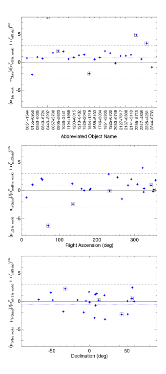
Figure 3: Comparison of the astrometric results from this paper to those presented in Gaia DR2 for the twenty-five objects (blue stars) in common. Mean offsets along the $y$-axis are shown by the dotted blue line; the dashed black lines show 3$\sigma$ excursions. Objects with $\chi^{2}_{\nu}$ values of 1.5 or greater are marked by squares and are not included in the computation of the mean.

The objects whose Gaia parallaxes we are using for comparison in Figure 3 are among the reddest and faintest objects that Gaia can detect. We can test whether the offsets seen between Gaia and our Spitzer results are pointing to an issue with the Gaia parallaxes themselves by comparing other Gaia parallaxes to independent literature values. Figure 14 illustrates this using parallaxes from Dahn et al. (2002), Dieterich et al. (2014), Winters et al. (2015), and Bartlett et al. (2017). Most of these parallaxes were measured by ground-based CCD programs, with the exception of those from Winters et al. (2015), who presented weighted parallax results using ground-based astrometry measured from photographic plates, CCDs, and infrared arrays as well as astrometry from Hipparcos. In our figure, care was taken not to double count results, so any data from Winters et al. (2015) that were included in the other references were removed.

These astrometric offsets with respect to Gaia are plotted as a function of apparent $G_{RP}$ magnitude in the top panel of Figure 14. As $G_{BP}$ is known to be systematically underestimated for the reddest objects in Gaia (Smart et al. 2019) – which in turn affects the $G_{BP}-G_{RP}$ color – we instead use absolute Gaia $G$-band magnitude in the bottom panel as a proxy for color. Colors like $B-R$ directly correlate with $M_{G}$ (or $M_{V}$) magnitudes across M and L dwarf spectral types (Pecaut & Mamajek 2013; Dieterich et al. 2014). The two panels also show a small bias between these published parallax values and those of Gaia, and the bias has the same sign as that seen in the Spitzer-to-Gaia comparison in Figure 3. Moreover, the two panels in Figure 14 suggest that there is a tendency for this bias to increase with fainter apparent magnitude and/or redder color.

The cause for this bias, and whether it highlights an unknown issue with the faintest Gaia astrometry, is unknown. Smart et al. (2019) compared a larger list of previously published parallaxes to those of Gaia DR2 and also found a difference. They concluded that the discrepancy could be reconciled if either the uncertainties in the (heterogeneous) ground-based parallaxes or the Gaia uncertainties themselves were increased. Given that our new set of homogeneous Spitzer astrometry shows a similar discrepancy as previous ground-based measurements suggests that the Gaia uncertainties are underestimated.

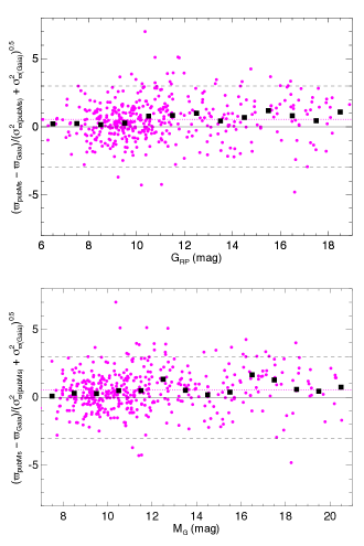
Figure 4: Comparison of the Gaia DR2 astrometric results to other published astrometry for a wider range of spectral types (M0 to L8) than that shown in Figure 3. Mean offsets along the $y$-axis are shown by the dotted magenta line; the dashed black lines show 3$\sigma$ excursions. Black squares show the median values along integral magnitude intervals in apparent $G_{RP}$ magnitude (top panel) and absolute $G$ magnitude (bottom panel). Trends suggest that the median offset increases with fainter apparent magnitude and with fainter absolute magnitude (which is used here as a proxy for color).

4.3 Comparison of Spitzer+unWISE to Pure-Spitzer Results

Above, we hypothesized that the small offset seen in the parallax differences with respect to Gaia would shrink if the Gaia uncertainties were found to be underestimated. Another possibility, which we will dispel here, is that our own measurement technique has introduced a small bias.

The Spitzer parallax measurements used in Figure 3 were supplemented with data from unWISE in order to extend the astrometric time baseline. These objects, although they are among the faintest that Gaia can measure, are the brightest objects in the Spitzer program. For this reason, their high-S/N Spitzer data alone are sufficient to obtain quality parallaxes, so we have performed a special "Spitzer only" reduction to ascertain whether or not the inclusion of the unWISE data has led to a bias. A comparison of the reductions with and without the unWISE data is shown in Figure 5. As expected, no significant difference is present, a bias having been detected only at the 0.2$\sigma$ level.

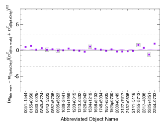
Figure 5: Comparison of the astrometric results from this paper to special astrometric runs for which the ancillary unWISE data are not used, for the twenty-five objects (purple squares) in common to this work and Gaia DR2. Mean offsets along the $y$-axis are shown by the dotted purple line; the dashed black lines show 3$\sigma$ excursions. Objects with $\chi^{2}_{\nu}$ values of 1.5 or greater are ringed by an open square and are not included in the computation of the mean.

4.4 Comparison to Best et al. (2020)

As this paper was being written, the parallax compilation of Best et al. (2020) became available, allowing us to do a comparison of our Spitzer results to another independent set of astrometry. This comparison is shown in Figure 6. The offsets seen are at the 0.8$\sigma$ ($\Delta{\varpi_{abs}}=4.3$ mas), 0.5$\sigma$ ($\Delta{\mu_{\alpha}}=1.6$ mas yr^-1), and 0.4$\sigma$ ($\Delta{\mu_{\delta}}=1.1$ mas yr^-1) levels for the top, middle, and bottom panels, respectively. Whereas our Spitzer parallaxes are slightly larger (by 0.8$\sigma$) than those of Gaia, Best et al. (2020) find that their UKIRT parallaxes are slightly smaller (by 1.6$\sigma$) than those of Gaia. Curiously, Best et al. (2020) also conclude that either their parallax uncertainties or those of Gaia are underestimated, at least the third such case in the recent literature to suggest that Gaia astrometric uncertainties may be too small for L and T dwarfs.

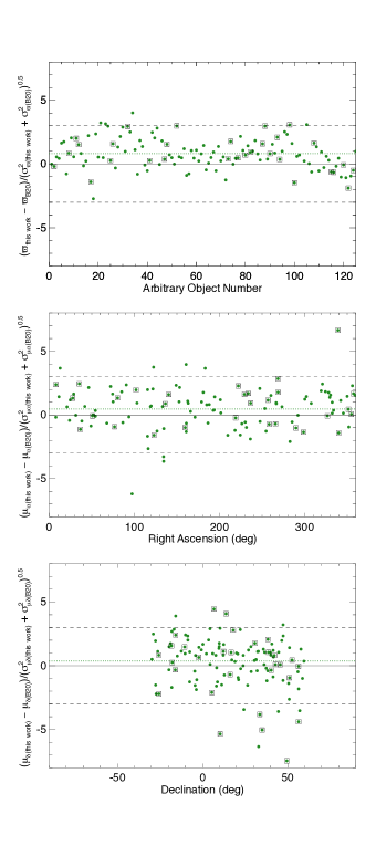
Figure 6: Comparison of the astrometric results from this paper to those from Best et al. (2020), for the 124 objects (green points) in common. Mean offsets along the $y$-axis are shown by the dotted green line; the dashed black lines show 3$\sigma$ excursions. Objects with $\chi^{2}_{\nu}$ values of 1.5 or greater in either work are marked by squares and are not included in the computation of the mean.

5 Supporting Data

Distance is only one of the important quantities needed when characterizing sources for the mass function analysis. Photometry across the optical through mid-infrared bands is needed to better assess the temperature of each source, which is needed when building a mass function that is tied to $T_{\rm eff}$ as the "observable" parameter. Spectroscopy is another powerful tool, and the most reliable one when assessing the small fraction of sources that have unusual features. These oddities complicate our ability to assign objects to the correct $T_{\rm eff}$ bins because their colors and spectral types follow relations that are different from the bulk of normal, single objects. For example, one oddity identifiable through spectroscopy is low metallicity, which may indicate an older subdwarf (e.g., Zhang et al. 2017). Another is low-gravity, which may indicate that the object is unusually young since it has yet to contract to its final, equilibrium radius (e.g., Faherty et al. 2016). Yet another is unresolved binarity, particularly at the L/T transition where spectroscopic blending of features makes composite spectra easier to distinguish (e.g., Burgasser, et al. 2010b). In the subsections that follow, we describe the data acquisition and reduction implemented for our photometric and spectroscopic follow-up campaigns. A compilation of our photometric, spectroscopic, and astrometric data is listed in Table 17, which is described in the Appendix.

5.1 Photometry

5.1.1 Facilities with 1-2.5 Micron Capability

The large-area archives searched for existing data were the Two Micron All-Sky Survey (2MASS; Skrutskie et al. 2006), the various UKIRT-based surveys being done with the Wide-field Camera (WFCAM; Casali et al. 2007) as part of the UKIRT Infrared Deep Sky Survey (UKIDSS; Lawrence et al. 2007), and the various surveys being done with the Visible and Infrared Survey Telescope for Astronomy (VISTA; Emerson et al. 2006) using the VISTA Infrared Camera (VIRCAM; Dalton et al. 2006). The WFCAM archives searched were those of the UKIDSS Large Area Survey (ULAS), the UKIDSS Galactic Plane Survey (UGPS; Lucas et al. 2008), the UKIDSS Galactic Clusters Survey (UGCS), and the UKIRT Hemisphere Survey (UHS; Dye et al. 2018). The VISTA-based survey data searched were those of the VISTA Hemisphere Survey (VHS) and the VISTA Variables in the Via Lactea (VVV; Minniti et al. 2010). Data were examined using the online WFCAM Science Archive and VISTA Science Archive.

Given the complex spectral energy distributions of L, T, and Y dwarfs, care needs to be taken with regards to filter systems. The two filter systems employed by these near-infrared surveys are those of 2MASS and the Maunakea Observatories (MKO; Tokunaga et al. 2002). Because of bandpass differences between these systems, the magnitude measured in, for example, the 2MASS $J$ filter may differ appreciably from the magnitude of the same L, T, or Y dwarf measured in MKO $J$. As a result, we report $J$ magnitudes in both. The $H$-band filter bandpasses are essentially identical between 2MASS and MKO, so a single $H$-band magnitude is reported. The 2MASS $K_{S}$-band and MKO $K$ band are also reported separately. (Note that none of these large-area surveys uses the MKO version of the $K_{S}$ filter.)

Per the recommendations given at http://horus.roe.ac.uk/vsa/ dboverview.html, we selected magnitudes with the string AperMag3 from both the WFCAM and VISTA Science Archives. For merged catalogs with multiple data sets per band, we chose the individual-epoch AperMag3 magnitude with the smallest uncertainty. Magnitudes combined over multiple epochs were avoided; because most of our objects have high motions, these combined magnitudes are generally incorrect because one epoch of blank sky has been averaged into the combined magnitude. That is, the catalog’s cross-matching between epochs is done purely on position, not on source identification.

For sources not covered or detected by these large-area surveys, we obtained follow-up photometry using the 2MASS camera (Milligan et al. 1996) on the 1.5 m Kuiper Telescope on Mt. Bigelow, Arizona; the NOAO Extremely Wide Field Infrared Imager (NEWFIRM; Swaters et al. 2009) at the 4 m Victor M. Blanco Telescope on Cerro Tololo, Chile; FLAMINGOS-2 (Eikenberry et al. 2006) on the 8.1 m Gemini-South Telescope on Cerro Pachón, Chile; the Persson’s Auxiliary Nasmyth Infrared Camera (PANIC; Martini et al. 2004) at the 6.5 m Magellan Baade Telescope at Las Campanas Observatory, Chile; the 1.3 m Peters Automated Infrared Imaging Telescope (PAIRITEL; Bloom et al. 2006) on Mt. Hopkins, Arizona; the Wide-field Infrared Camera (WIRC; Wilson et al. 2003b) at the 5 m Hale Telescope at Palomar Mountain, California; and the Ohio State Infrared Imager/Spectrometer (OSIRIS) at the 4.1 m Southern Astrophysical Research Telescope (SOAR) located at Cerro Pachón, Chile. Data acquisition and reduction from these instruments are described in Kirkpatrick et al. (2011) except those for FLAMINGOS-2, which are described in Meisner et al. (2020a).

5.1.2 Facilities with 3-5 Micron Capability

In Table 17, we have used the CatWISE2020 Catalog and Reject Table (Marocco et al. 2020) as the primary source of photometry in the 3-5 $\mu$m range. Specifically, we used the W1 and W2 magnitudes computed by the moving solutions (w1mpro_pm and w2mpro_pm) because these should be more accurate than photometry from the stationary solution given the high motions of our objects and the long, eight-year time baseline covered by the CatWISE2020 data. For comparison, we have also listed photometry (including W3) from the AllWISE Source Catalog and Reject Table. For AllWISE, we selected values from the stationary solution since these should be more stable than the moving solutions, as these were based on fragile motions measured over only a six-month time baseline. (For objects lacking AllWISE detections, the stationary solution from CatWISE2020 was used instead, as noted in the table.)

Table 17 also contains Spitzer/IRAC photometry in ch1 and ch2. Data from both our photometric follow-up and astrometric monitoring programs were used. For the latter programs, which had many epochs of ch2 data, the PRF-fit photometry from each individual epoch was used; the reported magnitude is that resulting from the weighted mean flux. We also searched for ancillary data in the Spitzer Heritage Archive to further supplement our ch1 and ch2 measurements. Those ancillary data sets are listed in Table 8. We have reduced those data using the same mosaic portion of our astrometric pipeline, and report the resulting PRF-fit magnitudes in Table 17. In these reductions, we used the PRF suite applicable to the phase of the mission, either cryogenic or warm, during which the data were taken. For targets in campaigns using IRAC’s "sweet spot" (Ingalls et al. 2012), we took only a portion of the resulting AORs since there is an enormous amount of data available; specfically, we selected a set of nine consecutive AORs toward the beginning of the campaign, another nine toward the middle, and another nine toward the end, and used those to build the mosaic needed for our pipeline.

Table 8: Ancillary Spitzer Photometry

Object	AOR	Bands	Program	PI
(1)	(2)	(3)	(4)	(5)
2MASS 0045+1634	67432448	1	14019ss	Vos
$\cdots$	67433472	2	$\cdots$	$\cdots$
WISE 0047+6803	58386688	1	12112ss	Allers
2MASS 0103+1935	43345408	1	80179ss	Metchev
$\cdots$	45626112	2	$\cdots$	$\cdots$
SDSS 0107+0041	10374912	1,2	3136*	Cruz
SIMP 0136+0933	21967360	1,2	40076*	Mainzer
2MASS 0144-0716	10375424	1,2	3136*	Cruz
2MASS 0251-0352	10376448	1,2	3136*	Cruz
WISE 0323+5625	32888832	1	61070	Whitney
$\cdots$	32902912	2	$\cdots$	$\cdots$
2MASS 0326-2102	25362944	1,2	50059*	Burgasser
2MASS 0340-6724	53291776	1	11174ss	Metchev
$\cdots$	53291520	2	$\cdots$	$\cdots$
2MASS 0355+1133	25363712	1,2	50059*	Burgasser
WISE 0401+2849	61990912	1	13006	Trilling
2MASS 0407+1514	12619008	1,2	35*	Fazio
2MASS 0421-6306	43338496	1	80179ss	Metchev
$\cdots$	45384960	2	$\cdots$	$\cdots$
2MASS 0439-2353	10377472	1,2	3136*	Cruz
2MASS 0443-3202	25363456	1,2	50059*	Burgasser
2MASS 0445-3048	10377728	1,2	3136*	Cruz
WISE 0457-0207	53278464	1	11174ss	Metchev
$\cdots$	53277952	2	$\cdots$	$\cdots$
PSO 0506+5236	67439360	1	14128ss	Faherty
2MASS 0512-2949	53291008	1	11174ss	Metchev
$\cdots$	53290752	2	$\cdots$	$\cdots$
2MASS 0523-1403	10377984	1,2	3136*	Cruz
WISE 0607+2429	50990336	1	10167ss	Gizis
$\cdots$	50990080	2	$\cdots$	$\cdots$
2MASS 0624-4521	10378240	1,2	3136*	Cruz
2MASS 0641-4322	50921984	1,2	10098	Stern
2MASS 0700+3157	10378496	1,2	3136*	Cruz
WISE 0715-1145	39058944	1	61071	Whitney
$\cdots$	39075584	2	$\cdots$	$\cdots$
2MASS 0755-3259	38996736	1	61071	Whitney
$\cdots$	39031808	2	$\cdots$	$\cdots$
SDSS 0809+4434	67435776	1,2	14128ss	Faherty
SDSS 0830+4828	10379008	1,2	3136*	Cruz
SDSS 0858+3256	21984768	1,2	40198*	Fazio
SDSS 0909+6525	21985280	1,2	40198*	Fazio
WISE 0920+4538	19064832	1,2	30854*	Uchiyama
SIPS 0921-2104	10380288	1,2	3136*	Cruz
2MASS 0949-1545	21985792	1,2	40198*	Fazio
2MASS 1022+5825	10380800	1,2	3136*	Cruz
SDSS 1043+1213	43336448	1	80179ss	Metchev
$\cdots$	45622784	2	$\cdots$	$\cdots$
SDSS 1045-0149	10381056	1,2	3136*	Cruz
SDSS 1048+0111	10381312	1,2	3136*	Cruz
WISE 1049-5319	48640512	1,2	90095	Luhman
2MASS 1051+5613	10381568	1,2	3136*	Cruz
2MASS 1122-3512	43331072	1	80179ss	Metchev
$\cdots$	45621504	2	$\cdots$	$\cdots$
2MASS 1126-5003	21981952	1,2	40198*	Fazio
2MASS 1213-0432	10382336	1,2	3136*	Cruz
SDSS 1214+6316	13778688	1,2	244*	Metchev
SDSS 1219+3128	53295104	1	11174ss	Metchev
$\cdots$	53294848	2	$\cdots$	$\cdots$
Gl 499C	53289984	1	11174ss	Metchev
$\cdots$	53289472	2	$\cdots$	$\cdots$
2MASS 1315-2649	15033856	1,2	20716*	Gizis
2MASS 1324+6358	13777920	1,2	244*	Metchev
DENIS 1425-3650	10383104	1,2	3136*	Cruz
2MASS 1448+1031	10383360	1,2	3136*	Cruz
Gaia 1713-3952	45999616	1	80253	Whitney
$\cdots$	45986304	2	$\cdots$	$\cdots$
VVV 1726-2738	21306368	1,2	30570*	Benjamin
2MASS 1731+2721	10384128	1,2	3136*	Cruz
WISE 1741-4642	67446272	1	14128ss	Faherty
2MASS 1750-0016	53283840	1	11174ss	Metchev
$\cdots$	53283072	2	$\cdots$	$\cdots$
SDSS 1750+4222	21986048	1,2	40198*	Fazio
2MASS 1753-6559	10384384	1,2	3136*	Cruz
2MASS 1807+5015	10384640	1,2	3136*	Cruz
WISE 1809-0448	54359040	1	11174ss	Metchev
$\cdots$	54358784	2	$\cdots$	$\cdots$
2MASS 1821+1414	43343616	1	80179ss	Metchev
$\cdots$	45625344	2	$\cdots$	$\cdots$
2MASS 1828-4849	12618496	1,2	35*	Fazio
Gaia 1831-0732	12109824	1	146*	Churchwell
$\cdots$	12105984	2	$\cdots$	$\cdots$
WISE 1906+4011	47929088	1	90152ss	Gizis
$\cdots$	47929344	2	$\cdots$	$\cdots$
Gaia 1955+3215	39262208	1,2	61072	Whitney
2MASS 2002-0521	67453440	1	14128ss	Faherty
WISE 2030+0749	53278208	1	11174ss	Metchev
$\cdots$	53277440	2	$\cdots$	$\cdots$
DENIS 2057-0252	10385408	1,2	3136*	Cruz
PSO 2117-2940	67446784	1	14128ss	Faherty
2MASS 2139+0220	10385664	1,2	3136*	Cruz
2MASS 2148+4003	22144256	1,2	284*	Cruz
2MASS 2151-2441	25364736	1,2	50059*	Burgasser
2MASS 2152+0937	10385920	1,2	3136*	Cruz
2MASS 2209-2711	35348480	1,2	61009	Freedman
DENIS 2252-1730	42482944	1,2	80183	Dupuy
2MASS 2331-4718	12619264	1,2	35*	Fazio

Note. — Program numbers followed by an asterisk were part of the Spitzer cryogenic mission and those with a suffix of "ss" used the IRAC "sweet spot".

5.2 Spectroscopy

We have obtained near-infrared spectra of some of the objects believed to lie within the 20-pc volume that lacked spectral types in the literature. These are listed in Table 9. Details on the observing runs and data reduction methods are given in the subsections below.

Table 9: Spectroscopic Follow-up

Object	Instrument	Obs. Date (UT)	Spec. Type
(1)	(2)	(3)	(4)
CWISE 0027$-$0121	Magellan/FIRE	2018 Dec 01	T9
CWISE 0041$-$4019	Magellan/FIRE	2018 Sep 23	T8 pec
CWISE 0115$-$4616	Magellan/FIRE	2018 Dec 01	T6
CWISE 0119$-$4937	Magellan/FIRE	2018 Dec 01	T7
CWISE 0119$-$4502	Magellan/FIRE	2018 Dec 01	T8
CWISE 0310$-$5733	Magellan/FIRE	2020 Feb 14	T5
Gaia 0412$-$0734	Keck/NIRES	2018 Sep 01	L2 pec (composite?)
$\cdots$	$\cdots$	2018 Nov 17	$\cdots$
CWISE 0424+0002	Magellan/FIRE	2019 Dec 12	T9:
CWISE 0433+1009	Keck/NIRES	2019 Dec 19	T8
CWISE 0514+2004	IRTF/SpeX	2018 Nov 25	T0.5
CWISE 0540$-$1802	CTIO/ARCoIRIS	2018 Apr 01	T5
CWISE 0601+1419	IRTF/SpeX	2018 Nov 25	T2.5
CWISE 0602$-$4035	Magellan/FIRE	2017 Dec 03	T5.5
CWISE 0613+4808	LDT/NIHTS	2019 Nov 13	T5
CWISE 0620$-$3006	Magellan/FIRE	2017 Dec 06	T2.5
Gaia 0623+2631	IRTF/SpeX	2019 Mar 16	L3 pec (composite?)
CWISE 0627$-$3730	Magellan/FIRE	2017 Dec 03	T6.5
CWISE 0630$-$6002	Magellan/FIRE	2019 Dec 11	T7
Gaia 0640$-$2352	Keck/NIRES	2018 Oct 27	L5
CWISE 0647$-$1600	Magellan/FIRE	2017 Dec 03	T6
Gaia 0734$-$4330	Magellan/FIRE	2020 Feb 13	L7 blue
CWISE 0749$-$6827	Magellan/FIRE	2017 Dec 03	T8 (pec?)
CWISE 0804$-$0000	CTIO/ARCoIRIS	2018 Apr 03	T4
CWISE 0845$-$3305	Magellan/FIRE	2020 Feb 13	T7
WISE 0902+6708	IRTF/SpeX	2019 Jan 22	L7 pec (low-g)
WISE 0911+2146	Magellan/FIRE	2020 Feb 13	T9
CWISE 0917$-$6344	Magellan/FIRE	2020 Feb 14	L7
CWISE 0953$-$0943	IRTF/SpeX	2019 Jan 23	T5.5
CWISE 1130$-$1158	CTIO/ARCoIRIS	2018 Apr 02	sdT5?
CWISE 1137$-$5320	Magellan/FIRE	2018 Feb 02	T7
CWISE 1141$-$2110	Magellan/FIRE	2019 Dec 11	T9:
CWISE 1152$-$3741	CTIO/ARCoIRIS	2018 Apr 02	T7
Gaia 1159$-$3634	IRTF/SpeX	2019 Mar 16	M9.5
CWISE 1205$-$1802	CTIO/ARCoIRIS	2018 Apr 02	T8
CWISE 1315$-$4936	Magellan/FIRE	2018 Jan 02	T3
Gaia 1331$-$6513	CTIO/ARCoIRIS	2019 Jun 19	M9
WISE 1333$-$1607	Magellan/FIRE	2018 Feb 02	T9
CWISE 1630$-$0643	Magellan/FIRE	2020 Feb 13	T5
Gaia 1648$-$2913	IRTF/SpeX	2019 Mar 16	L5 pec (composite?)
CWISE 1650+5652	IRTF/SpeX	2018 Jun 16	T0
CWISE 1726$-$4844	Magellan/FIRE	2020 Feb 13	T2.5
Gaia 1807$-$0625	IRTF/SpeX	2019 Mar 16	M9 pec (composite?)
CWISE 1832$-$5409	CTIO/ARCoIRIS	2018 Apr 02	T7
Gaia 1836+0315	IRTF/SpeX	2019 Mar 16	L6 v. red
CWISE 2001$-$4136	Magellan/FIRE	2016 Aug 09	T5
CWISE 2012+7017	LDT/NIHTS	2019 Nov 13	T4.5
CWISE 2058$-$5134	CTIO/ARCoIRIS	2019 Jun 19	T0
WISE 2126+2530	Palomar/DBSP	2019 Jul 22	M8
CWISE 2138$-$3138	Keck/NIRES	2019 Oct 28	T8
CWISE 2344$-$4755	Magellan/FIRE	2018 Dec 01	T5.5

5.2.1 Palomar/DBSP

A single object, WISE 2126+2530, was observed on 2019 Jul 22 (UT) using the Double Spectrograph (DBSP; Oke & Gunn 1982) at the Hale 5m telescope on Palomar Mountain, California. The D55 dichroic was used to split the light near 5500 Å  (0.55 $\mu$m). The blue arm utilized the 600 line mm^-1 grating blazed at 4000 Å (0.40 $\mu$m), while the red arm utilized the 316 line mm^-1 grating blazed at 7500 Å (0.75 $\mu$m), producing continuous coverage from 3400 to 10250 Å (0.340 to 1.025 $\mu$m) at a resolving power of $\sim$1500. A 600s exposure was acquired through partly cloudy conditions. Standard reduction procedures, as outlined in section 3.1.1 of Kirkpatrick et al. (2016) were employed.

5.2.2 LDT/NIHTS

Two objects were observed on 2019 Nov 13 (UT) using the Near-Infrared High Throughput Spectrograph (NIHTS; Gustafsson et al. 2019) at the 4.3-meter Lowell Discovery Telescope (LDT) at Happy Jack, Arizona. The 1$\farcs$34-wide slit was used providing an average resolving power of 62 over the 0.9–2.5 $\mu$m wavelength range. A series of ten 120s exposures was obtained of both WISE 0613$+$4808 and WISE 2012$+$7017 at two different positions along the 10$\arcsec$-long slit. Flats and xenon arcs exposures were taken at the beginning of the night and the A0 V stars, HD 45105 and HD 207646, respectively, were obtained for telluric correction purposes. The data were reduced using the Spextool data reduction package (Cushing et al. 2004), and telluric correction and flux calibration were achieved following the technique described in Vacca et al. (2003).

5.2.3 Keck/NIRES

Four objects were observed over the nights of 2018 Sep 01, Oct 27, and Nov 17, and 2019 Oct 28 and Dec 19 (UT) using the Near-Infrared Echellette Spectrometer (NIRES; see, e.g., Wilson et al. 2004) at the W.M. Keck II telescope on Maunakea, Hawaii. Setup and reductions were identical to those described in Meisner et al. (2020b) and covered a spectral range of 0.94-2.45 $\mu$m at a resolving power of $\sim$2700. Note that the spectra for Gaia 0412$-$0734 were combined across nights.

5.2.4 CTIO/ARCoIRIS

Eight objects were observed over the nights of 2018 Apr 01-03 and 2019 Jun 19 (UT) using the Astronomy Research using the Cornell Infra Red Imaging Spectrograph (ARCoIRIS) at the Victor Blanco 4m telescope at the Cerro Tololo Inter-American Observatory (CTIO), Chile. Instrument setup and data reductions are identical to those detailed in Greco et al. (2019) and covered a spectral range of 0.8-2.4 $\mu$m at a resolving power of $\sim$3500.

5.2.5 IRTF/SpeX

Ten objects were observed over the nights of 2018 Jun 16, Nov 25, and 2019 Jan 22/23 and Mar 16 (UT) using SpeX (Rayner et al. 2003) at the NASA Infrared Telescope Facility (IRTF) on Maunakea, Hawaii. SpeX was used in prism mode with a 0$\farcs$8-wide slit to achieve a resolving power of R = 100-500 over the range 0.8-2.5$\mu$m. All data were reduced using Spextool (Cushing et al. 2004). A0 stars were used for the telluric correction and flux calibration steps following the technique described in Vacca et al. (2003).

5.2.6 Magellan/FIRE

Twenty-five objects were observed over the nights of 2016 Aug 09; 2017 Dec 03 and Dec 06; 2018 Jan 02, Feb 02, Sep 23, and Dec 01; 2019 Dec 11/12; and 2020 Feb 13/14 (UT) using the Folded-port Infrared Echellette (FIRE; Simcoe et al. 2008, 2010) at the 6.5m Walter Baade (Magellan I) telescope at Las Campanas Observatory, Chile. Observations were done in high-throughput prism mode with the 0$\farcs$6 slit, which gives a resolving power of R$\approx$450 covering 0.8-2.45 $\mu$m. Reductions followed the steps described in Meisner et al. (2020b).

5.3 Spectral Classification

The spectra were classified as follows. For the single optical spectrum of WISE 2126+2530 in Figure 7, we overplotted spectral standards from Kirkpatrick et al. (1997), which are based on the optical classification system of Kirkpatrick et al. (1991) and looked for the best match over the entirety of the spectral range. For near-infrared spectra in Figures 8 and 9, we also performed a best by-eye fit, but using the near-infrared standards established by Kirkpatrick et al. (2010) for the L dwarfs, Burgasser et al. (2006) for early-T through late-T, and Cushing et al. (2011) for late-T through early-Y. In total, we classify four objects as M dwarfs, eight as L dwarfs, and 38 as T dwarfs.

Figure 7: Spectrum of WISE 2126+2530 (black) compared to the spectrum of the M8 standard van Biesbroeck 10 (red) from Kirkpatrick et al. (2010). The flux of both objects is normalized to one at 8250 Å, a high-S/N portion of the spectrum free from telluric absorption.

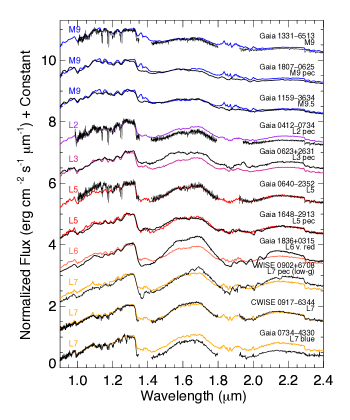
Figure 8: Spectra of M- and L-type dwarfs compared to the spectrum of the standard nearest in type. These near-infrared standards are taken from Kirkpatrick et al. (2010). The flux of all objects is normalized to one at 1.28 $\mu$m and offset by integral increments to ease comparison. Spectra of the target objects are in black and those of the standards in other colors. Our spectral classification of each target object is also shown in black and that of the nearest standard in other colors. Smoothing has been applied for some of the noisier target spectra.

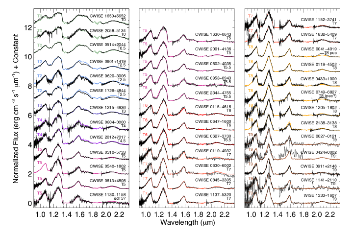
Figure 9: Spectra of WISE-selected objects compared to the spectrum of the standard nearest in type. These near-infrared standards are taken from Burgasser et al. (2006) and Cushing et al. (2011). See the caption to Figure 8 for other details.

6 Building the 20-pc Census

6.1 Objects to consider

The newly reduced Spitzer astrometry, along with published literature values, now enables a refinement of the 20-pc census. If an object has a trigonometric parallax measurement with an uncertainty $\leq$12.5%, we take that parallax at face value and retain the object if $\varpi_{obs}\geq 50$ mas. In this group there are a few objects that are worthy of special mention:

• CWISE 0536$-$3055: Based on the data available to Meisner et al. (2020a), those authors were unable to confirm the motion of this candidate. Using the Spitzer ch1 and ch2 magnitudes and color, our type and distance estimates suggest a [T9.5] dwarf at $\sim$17.4 pc. Our Spitzer astrometry from Table 5 gives a total proper motion of 37.4$\pm$13.7 mas yr^-1, which is different from zero only at the 2.7$\sigma$ level. More telling, however, is the high-quality absolute parallax, which is 78.1$\pm$3.8 mas (only 5% uncertainty; Table  5) based on Spitzer astrometric sampling with good coverage over the parallactic ellipse (Figure Set 1). CWISE 0536$-$3055 is therefore confirmed to be nearby and to fall within 20 pc of the Sun. This object represents a rare case in which the six-month parallactic motion (156.2 mas) is far (8.4$\times$) larger than the six-month proper motion (18.7 mas). Obtaining a radial velocity of this object would inform us whether CWISE 0536$-$3055 is coming toward our Solar System or away, and how that translates into a closest approach distance.

• WISE 0546$-$0959: As with CWISE 0536$-$3055 above, this T5 dwarf has an exceptionally small proper motion of 11.8$\pm$3.5 mas yr^-1 according to Best et al. (2020) or 10.3$\pm$2.5 mas yr^-1 according to our Spitzer astrometry, despite its large parallax of 50.4$\pm$3.6 (Best et al. 2020) or 57.5$\pm$3.9 mas (our Spitzer measurement). In this case, the six-month parallactic motion is $\sim$20$\times$ larger than the six-month proper motion.

• CWISE 1411$-$4811: Despite a robust Spitzer parallax value of 58.2$\pm$4.7 mas, this object has no measured spectral type. Its values of W1$-$W2 = 2.28$\pm$0.04 mag and M_ch2 = 13.10$\pm$0.18 mag (Table 17) suggest a type of [T6.5].

• WISE 1600$-$4543: This object has no measured spectral type, despite a robust parallax measurement of 74.7951$\pm$0.9190 mas from Gaia DR2. Using data in Table 17, we find that this source has M_W2 = 11.74$\pm$0.06 mag, which suggests [L9]. The color of $J_{2MASS}-$W2 = 2.62$\pm$0.04 mag suggests a type between mid-L and early-T.

• CWISE 1926$-$3429: Despite a robust Spitzer parallax value of 51.6$\pm$3.9 mas, this object has no measured spectral type. Values of ch1$-$ch2 = 0.98$\pm$0.03 mag and M_ch2 = 12.67$\pm$0.17 mag (Table 17) suggest a type of [T5.5].

In addition to objects with well measured parallaxes, there is another set of potential 20-pc members with poorer or non-existent parallax measurements that need additional scrutiny. The objects are listed in Table 10 and are (a) pulled from Table 1 or Tables 6-7, (b) are objects originally included in Spitzer program 14224 but dropped because of time restrictions, or (c) are previously published objects rediscovered by the CatWISE or Backyard Worlds teams for which initial estimates indicated distances within 23 pc of the Sun. We use a combination of photometric and spectrophotometric distance estimates to determine whether each object should be included in the 20-pc census. Namely, we use data from 20-pc census members with robust parallax measurements (uncertainties $\leq 12.5\%$) to construct three independent relations of M_J vs. $J-$W2 (valid for $J-$W2 $\geq$ 4.0 mag, or for 2.0 $\leq J-$W2 $<$ 4 mag if W1$-$W2 $\geq$ 2.2 mag), M_H vs. near-infrared spectral type (valid for all L, T, and Y spectral types), and M_ch2 vs. ch1$-$ch2 (valid for ch1$-$ch2 $\geq$ 0.4 mag). Using data provided in Table 17, we use the apparent magnitudes and colors of each object in Table 10 to estimate a distance from each relation, and then average the results to provide a final distance estimate. For some objects, there is not sufficient observational data for any of these relations – or the object has colors outside the range for which the relations are valid – so instead we use a M_W2 vs. W1$-$W2 relation (valid for W1$-$W2 $\geq$ 0.5 mag), also constructed from 20-pc members with robust parallax measurements, to provide a distance estimate.

Table 10: Other Objects Considered for the 20-pc Census

Object	Spec.	Spec.	Our	Pub.	Pub.	dest	dest	dest	dest	Final	Include	Remarks
name	type	type	$\varpi_{abs}$	$\varpi_{abs}$	$\varpi_{abs}$	$J$,W2	$H$,type	ch1,ch2	W1,W2	dest	in 20-pc
		ref.	(mas)	(mas)	ref.	(pc)	(pc)	(pc)	(pc)	(pc)	census?
(1)	(2)	(3)	(4)	(5)	(6)	(7)	(8)	(9)	(10)	(11)	(13)	(12)
CWISE 0027$-$0121	T9	T	54.2$\pm$7.9	$\cdots$	-	16.00	$\cdots$	17.47	$\cdots$	16.73	yes
2MASS 0034$-$0706	L4.3	D	$\cdots$	55.8$\pm$12.3	r	$\cdots$	32.03	$\cdots$	$\cdots$	32.03	no
CWISE 0043$-$3822	[T8.5]	T	38.1$\pm$15.7	$\cdots$	-	$\cdots$	$\cdots$	19.24	$\cdots$	19.24	yes
WISE 0048+2508	[T8.5]	m	$\cdots$	$\cdots$	-	12.48	$\cdots$	14.54	$\cdots$	13.51	yes
2MASS 0051$-$1544	L5	B	34.0$\pm$6.6	29.1$\pm$1.4	G	$\cdots$	$\cdots$	$\cdots$	$\cdots$	34.36	no
2MASS 0103+1935	L6(o)	K	35.9$\pm$5.7	46.9$\pm$7.6	F	$\cdots$	$\cdots$	$\cdots$	$\cdots$	21.32	no	see text
CWISE 0115$-$4616	T6	T	$\cdots$	$\cdots$	-	21.04	31.31	19.97	$\cdots$	24.11	no
CWISE 0119$-$4937	T7	T	$\cdots$	$\cdots$	-	18.11	39.29	20.47	$\cdots$	25.96	no
CWISE 0119$-$4502	T8	T	$\cdots$	$\cdots$	-	20.50	11.51	18.75	$\cdots$	16.92	yes
WISE 0132$-$5818	[T9]	m	27.2$\pm$7.3	$\cdots$	-	22.40	$\cdots$	21.67	$\cdots$	22.04	no
WISE 0135+1715	T6	k	65.3$\pm$10.0	46.7$\pm$3.5	W	$\cdots$	$\cdots$	$\cdots$	$\cdots$	21.41	no
WISE 0138$-$0322	T3	J	38.5$\pm$6.4	43.9$\pm$2.9	W	$\cdots$	$\cdots$	$\cdots$	$\cdots$	22.78	no

Note. — (This table is available in its entirety in a machine-readable form in the online journal. A portion is shown here for guidance regarding its form and content.)

Note. — Reference code for infrared spectral type. Values in brackets are estimates, and the types for 2MASS 0103+1935 and 2MASS 0639$-$7418 are based on optical spectra: (B) Burgasser et al. 2010, (b) Burgasser, et al. 2010b, (C) Cruz, et al. 2007, (D) Bardalez Gagliuffi, et al. 2014, (F) Faherty et al. 2016, (G) Mace et al. 2013, (g) Greco et al. 2019, (i) Kirkpatrick et al. 2016, (J) Kirkpatrick et al. 2011, (j) Kirkpatrick et al. 2010, (K) Kirkpatrick et al. 2000, (k) Kirkpatrick et al. 2012, (M) Meisner et al. 2020a, (m) Meisner et al. 2020b, (R) Reylé et al. 2014, (S) Schneider et al. 2017, (T) this paper, (U) Burningham et al. 2013, (u) Burningham et al. 2010, (W) Best et al. 2015.

Note. — Reference code for published parallax: (c) Theissen et al. 2020, (F) Faherty et al. 2012, (G) Gaia Collaboration et al. 2018, (g) Gaia Collaboration et al. 2018 parallax for the primary is cited, (r) Smart et al. 2018, (W) Best et al. 2020.

We also provide spectral types in Table  10. For objects without measured spectral types, we provide type estimates by using the final distance estimate in the table combined with the object’s ch2 magnitude to provide an estimate of $M_{ch2}$. We then take data from 20-pc census members having robust parallax measurement (uncertainties $\leq 12.5\%$) to construct a relation of spectral type vs. $M_{ch2}$ (valid over the entire range needed, 10.5 $<M_{ch2}<$ 16.0 mag), and use this to predict the type. (A value of $M_{W2}$ is used as a proxy for $M_{ch2}$ when no ch2 magnitude is available.) These estimated types are enclosed within brackets in the table.

Several objects requiring special consideration are noted by "see text" under the Remarks column in Table  10. Those objects are discussed below:

• 2MASS 0103+1935: This optical L6 dwarf (Kirkpatrick et al. 2000) has two independent parallax measurements, both low quality, of 35.9$\pm$5.7 mas (Table 6) and 46.9$\pm$7.6 mas (Faherty et al. 2012). Given that both measures suggest a parallax below 50 mas, we consider this object to fall outside of 20 pc.

• CWISE 0212+0531: This object was announced in Meisner et al. (2020a), although those authors were not able to confirm the object’s motion. Based on the Spitzer ch1 and ch2 magnitudes and color, our spectral type and distance estimates suggest [$\geq$Y1] at $<$13.3 pc. Our Spitzer astrometry from Table 7 gives a total proper motion of 82.6$\pm$52.7 mas yr^-1, which is different from zero at only the 1.6$\sigma$ level. The resulting parallax is 24.7$\pm$16.3 mas, with one parallax factor being represented by only a single Spitzer data point (Figure Set 1). Because both the motion and parallax are insignificantly different from zero, and because the measured parallax is much smaller than the expected value, we consider this to be a background object.

• CWISE 0423$-$4019: Our Spitzer photometry suggests a [T9] dwarf at $\sim$16.5 pc. Our Spitzer parallax measurement of $-$11.7$\pm$6.9 mas and total proper motion of 3.8$\pm$3.3 mas yr^-1, however, show that this is a background object and not a nearby brown dwarf.

• CWISE 0424+0002: This object was announced in Meisner et al. (2020a), although those authors were not able to confirm the object’s motion. Our Spitzer astrometry from Table 7 gives a total proper motion of 208.7$\pm$35.0 mas yr^-1, which is different from zero at the 6.0$\sigma$ level. The resulting parallax is 37.4$\pm$11.7 mas, representing a 31% uncertainty, and there is only a single Spitzer data point at one of the maximum parallax factors (Figure Set 1). Our spectrum from Figure 8 confirms that it is nearby. Because the motion is confirmed but the trigonometric parallax is not yet credible, we use our (spectro)photometric distance estimates to place this object within 20 pc.

• CWISE 0442$-$3855: Our Spitzer photometry suggests a [T8.5] dwarf at $\sim$16.8 pc. Our Spitzer parallax measurement of $-$12.4$\pm$4.9 mas and total proper motion of 3.6$\pm$2.6 mas yr^-1, however, show that this is a background object and not a nearby brown dwarf.

• CWISE 0617+1945: Using the colors of this object in Table 17, we are unable to provide a distance estimate using any of our four preferred absolute magnitude relations. Using the MKO-based $JHK$ magnitudes from Table 17, the color-color plots presented in section 7.4 suggest that this is a late-L dwarf, which would indicate M_H = 13.8 mag and a distance of $\sim$7.5 pc. As further discussed in section 7.3, the object appears to have a co-moving companion to its north-east, which is faint enough that it does not strongly affect the distance estimate. We consider this pair to fall within 20 pc.

• ULAS 0745+2332: This object, discovered by Burningham et al. (2013), lies in very close proximity to a background star that complicated our Spitzer astrometric measurements, leading to a false, negative parallax (Table 7). This object is not detected in any of the various WISE catalogs consulted for Table 17. The discovery paper lists a T8.5 spectral type and estimated distance of $<$19.4 pc, so we include this object in the 20-pc census.

• WISE 0830+2837: This candidate Y dwarf from Bardalez Gagliuffi et al. (2020) is sufficiently red in its Spitzer colors to be a possible bridge source in T_eff between spectroscopically verified early-Y dwarfs and WISE 0855$-$0714. Given its estimated distance of $\sim$8.2 pc and our low-quality parallax of 90.6$\pm$13.7 mas, we consider this object to be well within 20 pc.

• CWISE 1008+2031: This object was announced in Meisner et al. (2020a), although those authors were not able to confirm the object’s motion. Our Spitzer astrometry from Table 7 gives a total proper motion of 215.3$\pm$51.5 mas yr^-1, which is different from zero at the 4.2$\sigma$ level. The resulting parallax is 37.1$\pm$15.1 mas, representing a 41% uncertainty, with the Spitzer astrometric sampling providing only a single point at one of the maximum parallax factors (Figure Set 1). Because the motion of this object confirms it as being nearby and our photometric distance estimates place it within 20 pc, we include it in the 20-pc census.

• WISE 1040+4503: This object was announced in Meisner et al. (2020a), although those authors were not able to confirm the object’s motion. Our Spitzer astrometry from Table 7 gives a total proper motion of 91.7$\pm$32.3 mas yr^-1, which is different from zero at the 2.8$\sigma$ level. The resulting parallax is 18.8$\pm$9.8 mas, representing a 52% uncertainty, with the Spitzer astrometric sampling providing only a single point at one of the maximum parallax factors (Figure Set 1). Given that the photometric distance estimate is outside of 20 pc and that a distance within 20 pc is not suggested by the available astrometry, we exclude this object from the 20-pc census. It may, in fact, be a background object.

• CWISE 1047+5457: Meisner et al. (2020a) estimated that this is a [Y0] dwarf at $\sim$21.7 pc. Our low-quality parallax value of 75.2$\pm$12.8 suggests that it is closer. One of the maximum parallax factors is sampled with only one Spitzer data point (Figure Set 1), but this together with the other data samples strongly suggest a parallax $>$50 mas. We consider this object to lie within 20 pc, although higher quality astrometry is clearly needed.

• CFBDS 1118$-$0640: This object, which is a common proper motion companion to the mid-M dwarf 2MASS J11180698$-$0640078, was included in our Spitzer parallax program through a mistake. Its spectral type of T2 was paired up incorrectly with the WISE magnitudes of the primary, resulting in a photometric distance of $<$20 pc. The Gaia DR parallax of the primary is 9.90$\pm$0.15 mas, and our Spitzer parallax of the companion T dwarf is 1.4$\pm$5.2 mas. This object is therefore excluded from the 20-pc census.

• CWISE 1130$-$1158: This object has wildly discrepant distance estimates, with those using colors predicting a value within 20 pc and the one using spectral type indicating a value well outside 20 pc. Our spectroscopic follow-up from section 5.2 suggests that this object has a peculiar spectrum, particularly a depressed $K$-band spectrum similar to that seen in other T-type subdwarfs (e.g., Pinfield et al. 2014a). We therefore classify this object as an sdT5?. Given its possible subdwarf status, neither the color-based nor type-based relations may be accurate. For now, we consider this object to fall outside 20 pc, but additional astrometry is needed.

• 2MASS 1158+0435: This is an optical and near-infrared sdL7 (Kirkpatrick et al. 2010) placed on the parallax program because distance estimates for L subdwarfs are not yet well established. Our Spitzer parallax value of 39.2$\pm$6.2 mas is based on a well-sampled parallactic ellipse (Figure Set 1), so we consider this object to lie outside of 20 pc.

• ULAS 1319+1209: Burningham et al. (2010) classify this object as T5 pec based on a T5 fit in the $J$ band and a T3 fit in the $H$ band. In preparing our list of target objects for the Spitzer parallax program, we mistook this object to be the bright proper motion star immediately to its north, which has an AllWISE value of W2 = 12.56$\pm$0.03 mag. This led to an incorrect distance estimate of $\sim$9 pc. Our Spitzer parallax (7.8$\pm$6.5 mas) was measured for this brighter star, Gaia DR2 3739496602924096000, not of the T dwarf. Investigating this further, we find that the Gaia star, which is not listed in SIMBAD, has a Gaia DR2 parallax of 9.22$\pm$0.11 mas and motions of $\mu_{RA}$ = $-$135.2$\pm$0.2 mas yr^-1 and $\mu_{Dec}$ = 3.8$\pm$0.2 mas yr^-1. The motion measured by Burningham et al. (2013) for the T dwarf is $\mu_{RA}$ = $-$120.9$\pm$16.0 mas yr^-1 and $\mu_{Dec}$ = $-$22.9$\pm$14.6 mas yr^-1 which is consistent within the uncertainties to those of the Gaia star. Murray et al. (2011) estimate the distance of ULAS 1319+1209 to be 75$\pm$12 pc and note that it might be a halo T dwarf, although Liu et al. (2011) contend that thick disk membership is more likely. Burningham et al. (2013) estimate that the T dwarf falls between 58.6 and 99.1 pc if it is a single object, and could be as distant as 140.0 pc if a binary. These higher values are consistent with the distance to the Gaia object at 108.5 pc. The Gaia star has teff_val = 3974K, which would correspond to a late-K dwarf, whose metallicity should be easily measurable. We believe that this may be a new benchmark system and a particularly valuable one since the T dwarf shows peculiarities that may or may not be linked to a lower metallicity.

• Gaia 1331$-$6513: This is another object, like CWISE 0536$-$3055 discussed above, that has a very low motion value given its proximity to the Sun ($\sim$16.0 pc). The total motion from Gaia DR2 is 21.2$\pm$0.3 mas yr^-1, meaning that the parallactic motion over six months is twelve times larger than the proper motion. A measurement of the radial velocity would inform us whether this object is coming toward the Sun or away from it and the timescale for closest approach to the Solar System.

• WISE 1355$-$8258: This object was announced in Schneider et al. (2016), and Kirkpatrick et al. (2016) noted its unusual near-infrared spectrum, which they tentatively interpreted to be an sdL5. Bardalez Gagliuffi et al. (2018) attempted to explain the spectrum as that of an unresolved binary but were unable to find a binary fit that provided a convincing explanation. They noted, however, a possible kinematic association with the AB Doradus Moving Group, despite finding no spectroscopic evidence of low-gravity. Their best guess for the distance is 27-33 pc. Using WISE astrometry, Theissen et al. (2020) measure a fragile parallax of 60$\pm$19 mas (32% error). Using a combination of 2MASS and WISE astrometry, E. L. Wright (priv. comm.) finds a still fragile parallax of 73$\pm$16 mas (22% error). For now, we consider this object to lie outside of 20 pc but encourage future astrometric monitoring in an effort to better understanding this intriguing object.

• CWISE 1446$-$2317: Marocco et al. (2020) show that the Spitzer colors of this object place it among the coldest Y dwarfs currently known. Our Spitzer parallax measurements of 95.6$\pm$13.9 mas, though somewhat fragile based on its poorly sampled parallactic ellipse (Figure Set 1), nonetheless strongly suggests proximity to the Sun. We include this object within the 20 pc census.

• CWISE 1458+1734: This object is from Meisner et al. (2020a), who suggest a spectral type of [T8] and distance of $\sim$21.6 pc. Our Spitzer parallax measurement of 1.3$\pm$7.2 mas (Table 7) is based on a fit to a well-sampled parallactic ellipse. The proper motion of this source is measured at high significance, 503.6$\pm$26.1 mas yr^-1 (Table 7), so the lack of a measurable parallax is puzzling. We have compared the UHS $J$-band image from 2013 May to our own $J$-band image taken from Palomar/WIRC in 2020 Jul (Figure 10) and confirm a motion along nearly the same position angle indicated by our astrometric fit in Figure Set 1. We note, however that the position angle of the motion vector is almost perfectly aligned with the major axis of the parallactic ellipse, meaning that an incorrect motion magnitude could easily erase the parallactic signature. We have performed a test of this hypothesis by determining what value of the total motion is needed to create a parallactic signature matching the distance estimate in Table 10 while also assuming that the motion direction measured by our Spitzer+unWISE astrometry is correct. We get the correct result if the total proper motion is reduced from 504 mas yr^-1 to $\sim$300 mas yr^-1. This hypothesis is supported by the fact that CWISE 1458+1734 is moving between – and is bracketed by – two background objects that themselves fall along nearly the same position angle as the proper motion, and it is thus conceivable the unWISE astrometry of the T dwarf is pulled southeastward at early epochs by blending from the southeast source and northwestward at later epochs by blending from the northwest source, thereby inflating the true motion value. Crude measurements of the astrometry from the images in Figure 10 give a proper motion of $\sim$305 mas yr^-1, confirming our hypothesis. Nevertheless, the photometric distance of this source places it just outside 20 pc, so it is not included in our 20-pc census.

  

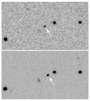
  Figure 10: Images at $J$-band for CWISE 1458+1734. (Top) The 2013 May image from UHS. (Bottom) Our 2020 Jul image from Palomar/WIRC. These images are 1$\times$0.5 arcmin with north up and east to the left. Arrows mark the location of CWISE1458+1734 and illustrate its motion over the 7.2-yr baseline.

• WISE 1534$-$1043: This object is from Meisner et al. (2020a), who note that its placement on the $J-$ch2 vs. ch1$-$ch2 color plot suggest it is a mid- to late-T subdwarf. As such, deriving a photometric distance estimate from relations that assume solar metallicity is useless. Too few late-T subdwarfs are known to enable a better distance estimate, particularly since we do not know if the object’s metallicity is similar to or more extreme than known T subdwarfs, so our Spitzer trigonometric distance measurement of 47.8$\pm$14.3 mas (Table 7) is the best current indicator, despite the large relative uncertainty of 30%. The object’s high proper motion, 2772.7$\pm$57.3 mas yr^-1, also points to an old, kinematically heated object. (At 20 pc, this would correspond to a tangential velocity of 263 km s^-1.) The $<$50mas parallax suggests that we exclude this object from the 20-pc census as we await additional astrometric measurements.

• WISE 1619+1347: This object was announced in Meisner et al. (2020b), although those authors were not able to confirm the object’s motion. Our Spitzer astrometry from Table 7 gives a total proper motion of 29.1$\pm$16.6 mas yr^-1, which is different from zero at only the 1.8$\sigma$ level. The resulting, negative parallax of $-$9.1$\pm$4.3 mas, is based on Spitzer astrometric data that sample the parallactic ellipse well (Figure Set 1). We therefore consider this to be a background object.

• CWISE 1827+5645: This object was re-discovered by high school student Justin Hong as part of the Summer Research Connection at Caltech in the summer of 2020. The object was first discovered during the original WISE mission and chosen for Spitzer follow-up in program 70062, where it was measured to have a ch1$-$ch2 color indicative of a late-T dwarf. Subsequent Palomar/WIRC $J$-band imaging indicated a magnitude of $\sim$19.0 mag, ruling out the possibility of its being a late-T dwarf. The object was rediscovered again by the Backyard Worlds team but was paired up with a $J$ = 19.33$\pm$0.17 mag UHS object – the same object seen in the Palomar imaging – and believed to be a more distant early-T dwarf based on its implied $J-$W2 color. This $J$-band source is, however, an interloper in the field and not the brown dwarf candidate itself. (The same background object also contaminates the proper motion measure from CatWISE2020.) The Spitzer photometry from 2012 is clean; this color, together with clear evidence of motion through the epochal coverage of WISE and NEOWISE images, indicates a [T9.5] dwarf just outside of the 20-pc census.

• CWISE 2058$-$5134: We are unable to provide a distance estimate to this object using any of our four preferred absolute magnitude relations. Our spectroscopic follow-up (Table 9) shows that this is a T0 dwarf, which would indicate M_JMKO = 14.5 mag using plots illustrated in the following section. This suggests a distance of $\sim$33.9 pc. We consider this object to fall outside of 20 pc.

6.2 The Resulting Census and Final Checks

Our final, full-sky census of L, T, and Y dwarfs within 20 pc of the Sun is presented in Table 11. This includes not only solivagant dwarfs within that distance but also all known L, T, and Y dwarf companions to earlier type stars within 20 pc. For objects confirmed or believed to be double or triple systems, each component that is an L, T, or Y dwarf is listed. The table lists each object’s discovery name, discovery reference, and optical and near-infrared spectral types (with reference), if measured. The table also lists the absolute parallax from Table 17 and the total proper motion, along with a reference for the astrometry. For cases in which either a spectral type or parallax is estimated, the estimated value is shown in brackets. (For the $T_{\rm eff}$ values listed in the penultimate column, the reader is referred to section 8.1.) The last column of the table is reserved for special notes. If a note of "[]" is listed, then that object’s listed parallax should be ignored in favor of the spectrophotometric estimate shown in brackets. If a note of "yng" or "sd" is listed, that object is discussed further in section 7.

Table 11: The Full-sky 20-pc Census of L, T, and Y Dwarfs (Known as of 2020 Oct)

Discovery	Disc.	Optical	Type	Infrared	Type	$\varpi_{abs}$	$\mu_{tot}$	Astrom.	$T_{\rm eff}$	Special
Designation	Ref.	Sp. Type	Ref.	Sp. Type	Ref.	(mas)	(mas yr-1)	Ref.	(K)	Note
(1)	(2)	(3)	(4)	(5)	(6)	(7)	(8)	(9)	(10)	(11)
SDSS J000013.54+255418.6	57	T5	214	T4.5	61	70.8$\pm$1.9	128.1$\pm$1.3	67	1227$\pm$95
GJ 1001B (000434$-$404405)	101	$\cdots$	$\cdots$	L5	102	82.0946$\pm$0.3768	1641.6$\pm$0.6	168	1613$\pm$134
GJ 1001C (000434$-$404405)	116	$\cdots$	$\cdots$	L5	102	82.0946$\pm$0.3768	1641.6$\pm$0.6	168	1613$\pm$134
WISE J000517.48+373720.5	8	$\cdots$	$\cdots$	T9	8	126.9$\pm$2.1	1033.6$\pm$1.4	0	555$\pm$88
2MASS J00145575$-$4844171	103	L2.5 pec	103	L2.5$\pm$1	104	50.1064$\pm$0.3898	915.1$\pm$0.5	168	1887$\pm$88
WISE J001505.87$-$461517.6	2	$\cdots$	$\cdots$	T8	2	75.2$\pm$2.4	802.5$\pm$1.5	0	656$\pm$88
2MASSW J0015447+351603	105	L2	105	L1.0	106	58.6085$\pm$0.3664	262.9$\pm$0.5	168	1898$\pm$88
CWISE J002727.44$-$012101.7	0	$\cdots$	$\cdots$	T9	0	54.2$\pm$7.9	452.9$\pm$3.3	0	566$\pm$79	[59.8]
WISE J003110.04+574936.3	20	$\cdots$	$\cdots$	L8	20	71.0$\pm$3.2	522.1$\pm$2.2	0	1460$\pm$88
WISE J003231.09$-$494651.4	2	$\cdots$	$\cdots$	T8.5	2	60.8$\pm$2.5	937.2$\pm$1.6	0	609$\pm$88
ULAS J003402.77$-$005206.7	27	$\cdots$	$\cdots$	T8.5	10	68.7$\pm$1.4	359.2$\pm$0.8	67	619$\pm$88
2MASS J00345157+0523050	3	$\cdots$	$\cdots$	T6.5	61	118.8$\pm$2.7	696.8$\pm$2.0	0	899$\pm$82
2MASSW J0036159+182110	107	L3.5	107	L4	124	114.4167$\pm$0.2088	910.0$\pm$0.4	168	1869$\pm$64
WISE J003829.05+275852.1	8	$\cdots$	$\cdots$	T9	8	88.2$\pm$2.0	93.2$\pm$1.4	0	545$\pm$88
Gl 27B (003921+211501)	28	$\cdots$	$\cdots$	T8	61	89.7891$\pm$0.0581	591.8$\pm$0.1	168	793$\pm$35
WISE J004024.88+090054.8	8	$\cdots$	$\cdots$	T7	8	69.8$\pm$1.5	74.5$\pm$2.2	1	850$\pm$88
CWISE J004143.77$-$401929.9	0	$\cdots$	$\cdots$	T8 pec	0	76.7$\pm$9.6	1532.9$\pm$2.1	0	686$\pm$79
CWISE J004311.24$-$382225.0	0	$\cdots$	$\cdots$	[T8.5]	0	[52.0]	392.5$\pm$4.0	0	624$\pm$79
2MASSW J0045214+163445	109	L2$\beta$	110	L2$\gamma$	118,175	65.0151$\pm$0.2274	362.1$\pm$0.5	168	2059$\pm$45	yng
WISE J004542.56+361139.1	8	$\cdots$	$\cdots$	T5	8	57.0$\pm$3.7	185.7$\pm$2.2	0	1021$\pm$88
WISEP J004701.06+680352.1	182	L7($\gamma$?)	175	L6-8$\gamma$	175	82.3$\pm$1.8	432.0$\pm$1.8	198	1230$\pm$27	yng
WISEU J004851.21+250814.9	233	$\cdots$	$\cdots$	[T8.5]	233	[74.0]	1231.0$\pm$17.8	0	624$\pm$79
WISEPC J004928.48+044100.1	4	$\cdots$	$\cdots$	L9	4	62.6$\pm$2.9	388.3$\pm$4.1	237	1256$\pm$88
WISE J004945.61+215120.0	8	$\cdots$	$\cdots$	T8.5	8	140.4$\pm$2.1	482.4$\pm$1.4	0	640$\pm$88
2MASS J00501994$-$3322402	29	$\cdots$	$\cdots$	T7	61	94.6$\pm$2.4	1485.1$\pm$2.1	67	836$\pm$71
CFBDS J005910.90$-$011401.3	30	$\cdots$	$\cdots$	T8.5	10	103.2$\pm$2.1	885.8$\pm$1.1	67	566$\pm$88
CWISEP J010527.69-783419.3	232	$\cdots$	$\cdots$	[T9]	232	87.2$\pm$4.4	331.5$\pm$12.3	0	566$\pm$79
SDSSp J010752.33+004156.1	122	L8	136	L6	124	64.13$\pm$4.51	634.5$\pm$7.1	68	1385$\pm$89
WISE J011154.36$-$505343.2	184	$\cdots$	$\cdots$	T1.5	184	57.3$\pm$4.7	498.6$\pm$1.8	0	1239$\pm$88
CWISE J011952.82$-$450231.2	0	$\cdots$	$\cdots$	T8	0	[59.1]	160.2$\pm$31.3	0	686$\pm$79
2MASS J01282664-5545343	111	L2	112	L1	111	54.0168$\pm$0.2345	258.7$\pm$0.8	168	1955$\pm$88
CFBDS J013302.27+023128.4	5	$\cdots$	$\cdots$	T8.5	5	53.1$\pm$2.6	617.0$\pm$1.8	0	661$\pm$88
SIMP J013656.57+093347.3	186	T2	214	T2	124	162.13$\pm$0.57	1237.9$\pm$0.2	172	1051$\pm$198	yng
CWISE J014308.73$-$703359.1	0	$\cdots$	$\cdots$	[T7.5]	0	[51.3]	271.7$\pm$32.0	0	751$\pm$79
2MASS J01443536-0716142	113	L5	113	L4.5	124	79.0319$\pm$0.6240	431.6$\pm$1.3	168	1628$\pm$88
WISE J014656.66+423410.0A	2	$\cdots$	$\cdots$	T9	2	51.7$\pm$2.0	452.8$\pm$1.3	0	566$\pm$79
WISE J014656.66+423410.0B	206	$\cdots$	$\cdots$	Y0	2	51.7$\pm$2.0	452.8$\pm$1.3	0	460$\pm$79
WISEPC J014807.25$-$720258.7	4	$\cdots$	$\cdots$	T9.5	4	91.7$\pm$3.4	1269.3$\pm$4.1	21,1	526$\pm$88
CWISE J014837.51$-$104805.6	0	$\cdots$	$\cdots$	[T8.5]	0	[66.8]	252.9$\pm$11.4	0	624$\pm$79
CWISE J015349.89+613746.3	0	$\cdots$	$\cdots$	[T0]	0	[52.4]	203.6$\pm$9.2	0	1254$\pm$79
DENIS-P J0205.4$-$1159A	138	$\cdots$	$\cdots$	[L5]	202	53.67$\pm$1.12	432.3$\pm$0.2	172	1613$\pm$134
DENIS-P J0205.4$-$1159B	203	$\cdots$	$\cdots$	[L8]	202	53.67$\pm$1.12	432.3$\pm$0.2	172	1335$\pm$134
DENIS-P J0205.4$-$1159[C]	202	$\cdots$	$\cdots$	[T0]	202	53.67$\pm$1.12	432.3$\pm$0.2	172	1254$\pm$79
WISEPA J020625.26+264023.6	4	$\cdots$	$\cdots$	L9 pec (red)	4	52.1$\pm$1.4	444.7$\pm$3.1	198	1281$\pm$88
2MASS J02132062+3648506C	80	$\cdots$	$\cdots$	T3	80	70.0180$\pm$0.2041	92.1$\pm$0.6	168	1175$\pm$88
2MASSI J0213288+444445	115	L1.5	115	$\cdots$	$\cdots$	51.6812$\pm$0.3832	154.8$\pm$0.7	168	2056$\pm$88
WISEPC J022322.39$-$293258.1	4	$\cdots$	$\cdots$	T7.5	4	80.7$\pm$2.6	946.1$\pm$1.9	1	706$\pm$88
WISEPA J022623.98$-$021142.8A	4	$\cdots$	$\cdots$	[T8]	1	51.1$\pm$2.3	522.6$\pm$2.3	237	686$\pm$79
WISEPA J022623.98$-$021142.8B	1	$\cdots$	$\cdots$	[T9.5]	1	51.1$\pm$2.3	522.6$\pm$2.3	237	511$\pm$79
CWISEP J023842.60-133210.7	232	$\cdots$	$\cdots$	[$\geq$Y1]	232	85.8$\pm$21.4	771.00$\pm$73.32	0	367$\pm$79	[55.6]
WISE J024124.73$-$365328.0	2	$\cdots$	$\cdots$	T7	2	53.1$\pm$2.5	281.3$\pm$1.5	0	868$\pm$88
2MASSI J0243137$-$245329	32	T5.5	214	T6	61	93.62$\pm$3.63	354.8$\pm$4.1	68	972$\pm$83
WISE J024714.52+372523.5	8	$\cdots$	$\cdots$	T8	8	64.8$\pm$2.0	92.6$\pm$1.8	237	656$\pm$88
2MASSI J0251148-035245	115	L3	115	L1	109	90.62$\pm$3.02	2149.7$\pm$0.9	169	1786$\pm$88
WISEPA J025409.45+022359.1	4,33	$\cdots$	$\cdots$	T8	4	146.1$\pm$1.5	2572.2$\pm$0.1	1	621$\pm$73
DENIS-P J0255$-$4700 (025503$-$470051)	81	L8	103	L9	61	205.3266$\pm$0.2545	1153.4$\pm$0.6	168	1290$\pm$78
2MASS J02572581$-$3105523	103	L8	103	L6	124	102.3651$\pm$0.6073	712.5$\pm$1.1	168	1311$\pm$88
WISEA J030237.53$-$581740.3	6	$\cdots$	$\cdots$	Y0:	6	59.9$\pm$3.3	87.8$\pm$5.0	0	460$\pm$79
WISE J030449.03$-$270508.3	7	$\cdots$	$\cdots$	Y0 pec	7	73.1$\pm$2.6	509.8$\pm$3.2	0	465$\pm$88
WISEA J030919.70$-$501614.2A	6	$\cdots$	$\cdots$	T7	236	62.2$\pm$2.8	566.8$\pm$1.9	0	819$\pm$79
WISEA J030919.70$-$501614.2[B]	1	$\cdots$	$\cdots$	[T7]	6	62.2$\pm$2.8	566.8$\pm$1.9	0	819$\pm$79
2MASS J03101401$-$2756452	194	L5:	194	L6.5	106	[50.2]	132.8$\pm$3.6	0	1465$\pm$134
WISEPA J031325.96+780744.2	4	$\cdots$	$\cdots$	T8.5	4	135.6$\pm$2.8	91.4$\pm$1.4	0	570$\pm$88
2MASS J03140344+1603056	117	L0	117	M9.4	106	73.4296$\pm$0.2757	248.6$\pm$0.5	168	2129$\pm$88
WISE J031624.35+430709.1	8	$\cdots$	$\cdots$	T8	8	74.7$\pm$2.1	439.0$\pm$1.3	0	520$\pm$88
2MASS J03185403$-$3421292	103	L7	103	L6.5	124	74.1$\pm$4.6	398.1$\pm$3.0	0	1344$\pm$107
CWISEP J032109.59+693204.5	232	$\cdots$	$\cdots$	[Y0.5]	232	68.5$\pm$4.0	993.5$\pm$13.9	0	412$\pm$79
WISE J032301.86+562558.0	184	$\cdots$	$\cdots$	L7	194	51.9$\pm$3.0	434.3$\pm$2.7	0	1493$\pm$88
WISEA J032309.12$-$590751.0	1	$\cdots$	$\cdots$	T7	236	72.1$\pm$2.9	735.6$\pm$2.1	0	819$\pm$79
WISEPC J032337.53$-$602554.9	4	$\cdots$	$\cdots$	T8.5	4	71.7$\pm$2.3	543.0$\pm$1.4	0	617$\pm$88
WISE J032517.69$-$385454.1	8	$\cdots$	$\cdots$	T9	8	60.2$\pm$3.5	308.4$\pm$2.1	0	556$\pm$88
WISE J032547.72+083118.2	8	$\cdots$	$\cdots$	T7	8	76.3$\pm$2.8	135.0$\pm$2.0	0	885$\pm$88
PSO J052.7214$-$03.8409 (033053$-$035027)	181	$\cdots$	$\cdots$	L9:	181	59.2$\pm$3.3	147.2$\pm$3.7	0	1197$\pm$88
WISE J033515.01+431045.1	8	$\cdots$	$\cdots$	T9	8	84.8$\pm$1.7	1142.3$\pm$0.9	0	495$\pm$88
WISE J033605.05$-$014350.4	8	$\cdots$	$\cdots$	Y0	22	99.8$\pm$2.1	1241.8$\pm$1.3	0	460$\pm$79
2MASS J03400942$-$6724051	120	$\cdots$	$\cdots$	L7::	120	107.1165$\pm$0.6174	598.0$\pm$2.3	168	1267$\pm$88
2MASS J03480772$-$6022270	34	$\cdots$	$\cdots$	T7	61	120.1$\pm$1.8	817.8$\pm$0.9	1	823$\pm$88
WISE J035000.32$-$565830.2	2	$\cdots$	$\cdots$	Y1	2	176.4$\pm$2.3	612.1$\pm$1.5	0	388$\pm$88
2MASS J03552337+1133437	117	L5$\gamma$	110	L3-L6$\gamma$	175	109.6451$\pm$0.7368	668.4$\pm$1.8	168	1478$\pm$58	yng
UGPS J03553200+4743588	83	$\cdots$	$\cdots$	[T6]	83	66.4$\pm$3.2	538.5$\pm$8.1	0	864$\pm$88
WISE J035934.06$-$540154.6	2	$\cdots$	$\cdots$	Y0	2	73.6$\pm$2.0	770.7$\pm$1.1	0	436$\pm$88
WISE J040137.21+284951.7	119	L3	119	L2.5	119	80.2894$\pm$0.2615	480.9$\pm$0.6	168	1816$\pm$88
CWISEP J040235.55-265145.4	232	$\cdots$	$\cdots$	[$\geq$Y1]	232	116.4$\pm$20.5	934.0$\pm$34.5	0	367$\pm$79	[82.5]
WISE J040418.01+412735.6	119	L2	119	L3 pec (red)	15	61.7516$\pm$0.4163	396.1$\pm$1.2	168	1780$\pm$88
2MASS J04070885+1514565	3	$\cdots$	$\cdots$	T5.5	124	56.74$\pm$2.07	237.7$\pm$0.7	200	1027$\pm$88
WISEPA J041022.71+150248.5	10	$\cdots$	$\cdots$	Y0	10	151.3$\pm$2.0	2418.3$\pm$1.1	0	451$\pm$88
CWISE J041102.41+471422.6	0	$\cdots$	$\cdots$	[T7]	0	[61.0]	463.1$\pm$35.8	0	819$\pm$79
Gaia J041246.85$-$073416.8	229	[L1:]	229	L2 pec	0	59.6888$\pm$0.3365	592.3$\pm$0.5	168	1963$\pm$134
WISE J041358.14$-$475039.3	8	$\cdots$	$\cdots$	T9	8	50.7$\pm$3.3	329.5$\pm$3.4	0	540$\pm$88
2MASS J04134574+3709087	133	[L1]	220	$\cdots$	$\cdots$	51.6559$\pm$0.3322	684.5$\pm$0.9	168	1965$\pm$88
2MASSI J0415195$-$093506	32	T8	197	T8	61	175.2$\pm$1.7	2278.2$\pm$1.2	67	677$\pm$56
WISEA J041743.13+241506.3	238	$\cdots$	$\cdots$	T6	236	[84.0]	470.5$\pm$16.0	0	965$\pm$79
2MASS J04210718$-$6306022	120	L5$\beta$	110	L5$\gamma$	275	50.0$\pm$3.3	265.0$\pm$2.9	0	1388$\pm$197	yng
SDSSp J042348.57$-$041403.5A	122	$\cdots$	$\cdots$	L6.5:	67	67.8584$\pm$1.5052	354.2$\pm$2.3	168	1465$\pm$134
SDSSp J042348.57$-$041403.5B	208	$\cdots$	$\cdots$	T2	67	67.8584$\pm$1.5052	354.2$\pm$2.3	168	1218$\pm$79
CWISE 042455.69+000221.5	232	$\cdots$	$\cdots$	T9:	0	[53.2]	208.7$\pm$35.0	0	566$\pm$79
2MASS J04250679$-$4255085	158	$\cdots$	$\cdots$	L8	158	[59.7]	156.1$\pm$7.2	0	1335$\pm$134
WISE J043052.92+463331.6	8	$\cdots$	$\cdots$	T8	8	96.1$\pm$2.9	961.4$\pm$2.6	0	516$\pm$88
2MASSI J0439010$-$235308	115	L6.5	115	L6	124	80.7917$\pm$0.5139	190.7$\pm$1.1	168	1290$\pm$82
2MASSI J0445538$-$304820	115	L2	115	$\cdots$	$\cdots$	61.9685$\pm$0.1843	449.7$\pm$0.5	168	1809$\pm$90
WISEPA J044853.29$-$193548.5	4	$\cdots$	$\cdots$	T5 pec	4	57.6$\pm$3.0	1179.5$\pm$1.3	0	950$\pm$88	sd
WISE J045746.08$-$020719.2	35	$\cdots$	$\cdots$	T2	35	82.0$\pm$2.9	140.4$\pm$3.7	237	1259$\pm$88
WISEPA J045853.89+643452.9A	11	$\cdots$	$\cdots$	T8.5	10	106.7$\pm$2.8	358.0$\pm$1.4	0	624$\pm$79
WISEPA J045853.89+643452.9B	56	$\cdots$	$\cdots$	T9.5	10	106.7$\pm$2.8	358.0$\pm$1.4	0	511$\pm$79
WISEPA J050003.05$-$122343.2	4	$\cdots$	$\cdots$	T8	4	84.6$\pm$2.2	724.8$\pm$2.5	237	614$\pm$88
2MASS J05002100+0330501	117	L4	117	L4.1	106	76.2093$\pm$0.3565	351.8$\pm$0.7	168	1793$\pm$72
WISEU J050305.68-564834.0	233	$\cdots$	$\cdots$	[$\geq$Y1]	233	98.3$\pm$3.9	812.1$\pm$13.7	0	367$\pm$79
PSO J076.7092+52.6087 (050650+523631)	181	$\cdots$	$\cdots$	T4.5	181	61.3$\pm$3.1	208.3$\pm$5.7	0	1135$\pm$88
WISE J050854.88+331920.8	16	L2	149	$\cdots$	$\cdots$	52.9819$\pm$0.6076	654.1$\pm$1.4	168	1850$\pm$88
2MASS J05103524$-$4208146	24	$\cdots$	$\cdots$	T5	24	53.8$\pm$2.4	592.1$\pm$1.5	200	1006$\pm$88
WISEPA J051317.28+060814.7	4	$\cdots$	$\cdots$	T6.5	4	70.8$\pm$1.5	433.0$\pm$1.0	1	916$\pm$88
CWISE J051427.35+200447.7	0	$\cdots$	$\cdots$	T0.5	0	[54.1]	103.8$\pm$10.0	0	1245$\pm$79
WISE J052126.29+102528.4	35	$\cdots$	$\cdots$	T7.5	35	150.2$\pm$3.0	492.1$\pm$3.5	0	727$\pm$88
UGPS J052127.27+364048.6	46	$\cdots$	$\cdots$	T8.5	46	122.2$\pm$1.6	1614.6$\pm$1.3	1	616$\pm$88
2MASSI J0523382-140302	115	L2.5	115	L5	109	78.3632$\pm$0.1855	193.4$\pm$0.4	168	1939$\pm$68
WISE J053516.80$-$750024.9	2	$\cdots$	$\cdots$	$\geq$Y1:	2	68.7$\pm$2.0	122.4$\pm$1.1	0	410$\pm$88
CWISEP J053644.82-305539.3	232	$\cdots$	$\cdots$	[T9.5]	0	78.1$\pm$3.8	37.4$\pm$13.7	0	511$\pm$79
SDSSp J053951.99-005902.0	121	L5	121	L5	122	78.5318$\pm$0.5707	359.9$\pm$1.1	168	1659$\pm$74
CWISE J054025.89$-$180240.3	0	$\cdots$	$\cdots$	T5	0	59.2$\pm$4.0	94.6$\pm$3.8	237	982$\pm$88
WISE J054047.00+483232.4	8	$\cdots$	$\cdots$	T8.5	8	69.4$\pm$2.1	678.8$\pm$1.3	0	606$\pm$88
WISEPA J054231.26$-$162829.1	4	$\cdots$	$\cdots$	T6.5	4	61.3$\pm$2.6	371.0$\pm$3.5	237	895$\pm$88
WISE J054601.19$-$095947.5	8	$\cdots$	$\cdots$	T5	8	50.4$\pm$3.6	11.7$\pm$3.5	237	1105$\pm$88
2MASS J05591914$-$1404488	51	T5	197	T4.5	124	97.28$\pm$0.59	661.5$\pm$0.2	172	1301$\pm$75
CWISE J060149.45+141955.2	0	$\cdots$	$\cdots$	T2.5	0	[54.3]	234.6$\pm$10.1	0	1209$\pm$79
2MASS J06020638+4043588	24	$\cdots$	$\cdots$	T4.5	24	76.4$\pm$3.1	324.0$\pm$2.1	0	985$\pm$88
LSR J0602+3910 (060230+391058)	123	L1	123	L1$\beta$	175	85.6140$\pm$0.1663	530.0$\pm$0.4	168	1857$\pm$133	yng
WISEP J060738.65+242953.4	119	L8	119	L9	20	136.9449$\pm$0.6553	572.7$\pm$1.4	168	1271$\pm$88
Gl 229B (061034$-$215200)	36	$\cdots$	$\cdots$	T7pec	61	173.6955$\pm$0.0457	731.8$\pm$0.2	168	927$\pm$77
WISEPA J061407.49+391236.4A	4	$\cdots$	$\cdots$	[T6]	1	53.7$\pm$1.7	529.3$\pm$1.2	1	965$\pm$79
WISEPA J061407.49+391236.4B	1	$\cdots$	$\cdots$	[T8]	1	53.7$\pm$1.7	529.3$\pm$1.2	1	686$\pm$79
WISE J061437.73+095135.0	8	$\cdots$	$\cdots$	T7	8	64.9$\pm$2.0	416.4$\pm$1.1	0	833$\pm$88
WISEA J061557.21+152626.1	22	$\cdots$	$\cdots$	T8.5	22	52.8$\pm$3.1	532.9$\pm$3.6	0	624$\pm$88
CWISE J061741.79+194512.8A	0	$\cdots$	$\cdots$	[L6.5]	0	[133.0]	119.8$\pm$5.5	0	1465$\pm$134
CWISE J061741.79+194512.8B	0	$\cdots$	$\cdots$	[T8:]	0	[133.0]	119.8$\pm$5.5	0	686$\pm$79
CWISE J062050.79$-$300620.8	0	$\cdots$	$\cdots$	T2.5	0	[54.6]	147.7$\pm$12.3	0	1209$\pm$79
WISEPA J062309.94$-$045624.6	4	$\cdots$	$\cdots$	T8	4	86.5$\pm$1.7	921.9$\pm$2.4	237	688$\pm$88
2MASS J06244595-4521548	117	L5	117	L5	124	81.6233$\pm$0.4986	378.4$\pm$1.5	168	1501$\pm$85
WISEPA J062720.07$-$111428.8	4	$\cdots$	$\cdots$	T6	4	74.8$\pm$3.6	338.1$\pm$1.6	1	1023$\pm$88
CWISEP J063428.10+504925.9	232	$\cdots$	$\cdots$	[Y0]	232	62.0$\pm$4.2	1192.4$\pm$19.2	0	460$\pm$79
2MASS J06411840-4322329	112	L1.5	112	L2.4:	106	51.2819$\pm$0.1930	666.6$\pm$0.5	168	1927$\pm$120
WISE J064205.58+410155.5	8	$\cdots$	$\cdots$	extr. red	8	62.6$\pm$3.1	383.1$\pm$1.7	0	1185$\pm$88
WISE J064336.71$-$022315.4	228	$\cdots$	$\cdots$	L8	228	71.9172$\pm$1.3761	223.0$\pm$3.4	168	1286$\pm$88
WISEA J064503.72+524054.1	233	$\cdots$	$\cdots$	[T8.5]	233	53.5$\pm$4.2	982.1$\pm$16.3	0	624$\pm$79
WISEA J064528.39$-$030247.9	6	$\cdots$	$\cdots$	T6	6	54.1$\pm$3.0	322.2$\pm$2.2	0	817$\pm$88
2MASS J06453153$-$6646120	133	sdL8	133	sdL8	133	53.8$\pm$2.9	1582.3$\pm$2.6	0	1369$\pm$88	sd
HD 46588B (064627+793504)	84	$\cdots$	$\cdots$	L9:	84	54.9292$\pm$0.1076	612.0$\pm$0.3	168	1257$\pm$88
WISE J064723.23$-$623235.5	12	$\cdots$	$\cdots$	Y1	12	99.5$\pm$1.7	393.9$\pm$0.9	0	393$\pm$88
WISEA J064750.85$-$154616.4	85	$\cdots$	$\cdots$	L9.5	85	62.7$\pm$3.3	178.4$\pm$3.0	0	1391$\pm$88
PSO J103.0927+41.4601 (065222+412736)	86	$\cdots$	$\cdots$	T0	86	57.6$\pm$3.3	41.0$\pm$3.2	0	1395$\pm$88
2MASSI J0652307+471034	115	L4.5	115	L6.5	124	110.31$\pm$0.29	181.7$\pm$0.1	172	1597$\pm$88
WISEPA J065609.60+420531.0	4	T2	214	T3	4	63.0$\pm$4.1	356.7$\pm$5.5	237	1235$\pm$88
2MASS J07003664+3157266A	125	L3	117	L3:	102	88.2790$\pm$0.3479	559.9$\pm$0.7	168	1838$\pm$134
2MASS J07003664+3157266B	117	L6.5	117	L6.5:	102	88.2790$\pm$0.3479	559.9$\pm$0.7	168	1465$\pm$134
2MASS J07003664+3157266[C]	180	L6.5::	180	$\cdots$	$\cdots$	88.2790$\pm$0.3479	559.9$\pm$0.7	168	1465$\pm$134
WISE J070159.79+632129.2	8	$\cdots$	$\cdots$	T3	8	52.6$\pm$3.0	263.0$\pm$1.4	0	1281$\pm$88
WISEA J071301.86$-$585445.2	6	$\cdots$	$\cdots$	T9	6	82.1$\pm$3.0	372.3$\pm$2.5	0	521$\pm$88
WISE J071322.55$-$291751.9	2	$\cdots$	$\cdots$	Y0	2	109.3$\pm$2.1	542.0$\pm$1.3	0	464$\pm$88
WISEA J071552.38-114532.9	126	$\cdots$	$\cdots$	L4 pec (blue)	126	55.5855$\pm$0.3446	803.3$\pm$0.8	168	1154$\pm$88
WISE 072003.20$-$084651.2B	238	$\cdots$	$\cdots$	[T5.5]	239	147.1$\pm$1.2	125.3$\pm$4.6	240	1183$\pm$88
UGPS J072227.51$-$054031.2	37	T9	4	T9	10	242.8$\pm$2.4	970.3$\pm$2.1	40	569$\pm$45
WISE J072312.44+340313.5	8	$\cdots$	$\cdots$	T9:	8	60.8$\pm$2.1	348.1$\pm$1.2	0	631$\pm$88
2MASSI J0727182+171001	32	T8	197	T7	61	112.5$\pm$0.9	1296.2$\pm$0.9	67	845$\pm$71
2MASS J07290002$-$3954043	24	$\cdots$	$\cdots$	T8 pec	24	126.3$\pm$8.3	1738.3$\pm$7.6	66	752$\pm$69	sd
WISE J073444.02$-$715744.0	2	$\cdots$	$\cdots$	Y0	2	74.5$\pm$1.7	569.0$\pm$0.9	0	462$\pm$88
SDSS J074149.15+235127.5	57	$\cdots$	$\cdots$	T5.5	124	73.2$\pm$3.4	343.8$\pm$2.2	0	909$\pm$88
SDSS J074201.41+205520.5	57	$\cdots$	$\cdots$	T5	124	63.5$\pm$3.1	400.3$\pm$1.1	0	958$\pm$102
WISEPA J074457.15+562821.8	4	$\cdots$	$\cdots$	T8	4	65.3$\pm$2.0	781.7$\pm$1.1	0	726$\pm$88
ULAS J074502.79+233240.3	19	$\cdots$	$\cdots$	T8.5	19	[$\geq$51.5]	$\cdots$	-	624$\pm$79
2MASSI J0746425+200032A	107	L0	128	$\cdots$	$\cdots$	81.9$\pm$0.3	378.5$\pm$0.3	170	2237$\pm$134
2MASSI J0746425+200032B	127	L1.5	128	$\cdots$	$\cdots$	81.9$\pm$0.3	378.5$\pm$0.3	170	2029$\pm$134
WISEPA J075003.84+272544.8	4	$\cdots$	$\cdots$	T8.5	4	68.4$\pm$3.4	783.2$\pm$2.7	1	583$\pm$88
WISEPA J075108.79$-$763449.6	4	$\cdots$	$\cdots$	T9	4	97.9$\pm$6.7	216.7$\pm$5.3	1	492$\pm$88
DENIS-P J0751164-253043	129	L1.5	129	L1.1	106	56.5689$\pm$0.1555	891.0$\pm$0.3	168	2083$\pm$64
WISE J075430.95+790957.8	8	$\cdots$	$\cdots$	extr. red	8	51.1$\pm$1.2	437.3$\pm$3.0	198	1248$\pm$88
2MASSI J0755480+221218	32	T6	197	T5	124	67.4$\pm$3.2	257.1$\pm$1.4	0	1001$\pm$88
HIP 38939B (075804$-$253735)	88	$\cdots$	$\cdots$	T4.5	88	54.1012$\pm$0.0386	437.8$\pm$0.1	168	1095$\pm$88
SDSS J075840.33+324723.4	57	T3	214	T2.5	124	101.3$\pm$3.3	400.9$\pm$1.5	0	1169$\pm$88
WISEPC J075946.98$-$490454.0	4	$\cdots$	$\cdots$	T8	4	90.7$\pm$2.1	447.1$\pm$1.1	0	666$\pm$88
CWISE J080556.14+515330.4	0	$\cdots$	$\cdots$	[T7.5]	0	[64.2]	578.0$\pm$28.3	0	751$\pm$79
WISEA J080622.22-082046.5	233	$\cdots$	$\cdots$	[T8]	233	82.2$\pm$9.0	1331.1$\pm$36.3	0	819$\pm$79
WISE J080700.23+413026.8	20	$\cdots$	$\cdots$	L8 pec	20	50.7$\pm$3.3	346.6$\pm$1.8	0	1383$\pm$88
WD 0806$-$661B (080714$-$661848)	65	$\cdots$	$\cdots$	[Y1]	1	51.9342$\pm$0.0195	442.8$\pm$0.1	168	377$\pm$88
WISE J081117.81$-$805141.3	8	$\cdots$	$\cdots$	T9.5:	8	99.1$\pm$7.7	293.4$\pm$6.9	21,1	479$\pm$88
DENIS J081730.0$-$615520	38	$\cdots$	$\cdots$	T6	38	191.5301$\pm$0.6037	1110.7$\pm$1.7	168	1004$\pm$91
WISEPA J081958.05$-$033529.0	4	T4	214	T4	4	71.4$\pm$2.2	250.5$\pm$1.0	200	1225$\pm$88
WISE J082000.48$-$662211.9	184	$\cdots$	$\cdots$	L9.5	184	56.1$\pm$3.4	355.9$\pm$2.9	0	1206$\pm$88
WISE J082507.35+280548.5	9	$\cdots$	$\cdots$	Y0.5	9	152.6$\pm$2.0	245.1$\pm$1.3	0	376$\pm$88
2MASSI J0825196+211552	105	L7.5	105	L7	124	93.19$\pm$0.59	581.1$\pm$0.2	172	1341$\pm$73
WISEA J082640.45$-$164031.8	15	$\cdots$	$\cdots$	L9	15	67.8$\pm$3.5	985.8$\pm$3.8	0	1263$\pm$88
SSSPM J0829-1309 (082834-130919)	130	L2	130	$\cdots$	$\cdots$	85.5438$\pm$0.1720	582.2$\pm$0.3	168	1983$\pm$88
SDSSp J083008.12+482847.4	122	L8	103	L9.5$\pm$1	124	76.42$\pm$3.43	1267.0$\pm$6.5	68	1258$\pm$97
WISEA J083011.95+283716.0	234	$\cdots$	$\cdots$	[$\geq$Y1]	234	90.6$\pm$13.7	2054.1$\pm$57.1	0	367$\pm$79	[121.4]
WISE J083337.83+005214.2	13	$\cdots$	$\cdots$	(sd)T9	13	79.7$\pm$3.1	1777.3$\pm$2.9	0	472$\pm$88	sd
2MASSI J0835425$-$081923	115	L5	115	L5	124	138.6098$\pm$0.2781	615.3$\pm$0.6	168	1754$\pm$112
CWISE J084506.51$-$330532.7	0	$\cdots$	$\cdots$	T7	0	[57.3]	1061.8$\pm$35.1	0	819$\pm$79
2MASSI J0847287-153237	115	L2	115	$\cdots$	$\cdots$	56.9235$\pm$0.3167	239.8$\pm$0.8	168	1794$\pm$81
WISE J085510.83$-$071442.5	14,16	$\cdots$	$\cdots$	[Y4]	1	439.0$\pm$2.4	8151.6$\pm$1.8	0	250$\pm$50
WISEPA J085716.25+560407.6	4	$\cdots$	$\cdots$	T8	4	85.3$\pm$2.1	754.9$\pm$1.3	0	671$\pm$88
SDSSp J085758.45+570851.4	122	L8	103	L8	175	71.2343$\pm$1.0255	565.5$\pm$2.3	168	1455$\pm$88
ULAS J085910.69+101017.1	64	$\cdots$	$\cdots$	T7	64	50.3$\pm$1.7	712.7$\pm$1.6	1	709$\pm$88
2MASSI J0859254$-$194926	115	L7:	120	L8	20	71.22$\pm$3.54	337.5$\pm$1.0	199	1374$\pm$100
CWISEP J085908.26+152527.1	232	$\cdots$	$\cdots$	[T8]	232	[53.2]	271.9$\pm$61.1	0	686$\pm$79
CWISEP J085938.95+534908.7	232	$\cdots$	$\cdots$	[Y0]	232	[53.8]	392.4$\pm$52.3	0	460$\pm$79
ULAS J090116.23$-$030635.0	39	$\cdots$	$\cdots$	T7.5	39	62.6$\pm$2.6	264.0$\pm$3.6	70	638$\pm$88
2MASSI J0908380+503208	115	L5	115	L6	124	95.8202$\pm$0.6983	628.6$\pm$2.2	168	1360$\pm$88
SDSS J090900.73+652527.2	53	$\cdots$	$\cdots$	T1.5	124	63.9$\pm$3.9	253.0$\pm$1.8	0	1146$\pm$88
CWISE J091105.02+214645.1	0	$\cdots$	$\cdots$	T9	0	[72.8]	667.0$\pm$2.5	0	566$\pm$79
2MASS J09153413+0422045A	117	L6:	209	$\cdots$	$\cdots$	54.8460$\pm$1.0970	112.9$\pm$2.8	168	1512$\pm$134
2MASS J09153413+0422045B	117	L7::	209	$\cdots$	$\cdots$	54.8460$\pm$1.0970	112.9$\pm$2.8	168	1420$\pm$134
CWISE J091735.38$-$634451.2	0	$\cdots$	$\cdots$	L7	0	[62.2]	110.0$\pm$8.8	0	1420$\pm$134
WISE J092055.40+453856.3	89	$\cdots$	$\cdots$	L9	8	79.4$\pm$3.9	856.6$\pm$4.8	237	1288$\pm$88
SIPS J0921$-$2104 (092114$-$210444)	117,131	L2	117	L4: (blue)	132,133	79.3128$\pm$0.2253	944.2$\pm$0.5	168	1930$\pm$88
CWISE J092503.20$-$472013.8	0	$\cdots$	$\cdots$	[Y0]	0	[93.3]	808.0$\pm$57.2	0	460$\pm$79
2MASSI J0937347+293142	32	T7	197	T6pec	61	162.84$\pm$3.88	1622.0$\pm$7.1	68	881$\pm$74	sd
CWISEP J093852.89+063440.6	232	$\cdots$	$\cdots$	[Y0]	232	67.9$\pm$13.8	792.9$\pm$50.6	0	460$\pm$79	[53.2]
2MASS J09393548$-$2448279A	29	$\cdots$	$\cdots$	[T8]	61	187.3$\pm$4.6	1191.7$\pm$3.4	71	686$\pm$79	sd
2MASS J09393548$-$2448279[B]	29	$\cdots$	$\cdots$	[T8]	61	187.3$\pm$4.6	1191.7$\pm$3.4	71	686$\pm$79
CWISEP J094005.50+523359.2	232	$\cdots$	$\cdots$	[$\geq$Y1]	232	66.4$\pm$12.2	491.2$\pm$51.9	0	367$\pm$79	[75.0]
WISE J094305.98+360723.5	18	$\cdots$	$\cdots$	T9.5	18	97.1$\pm$2.9	836.3$\pm$1.8	0	468$\pm$88
LHS 6176B (095047+011734)	40,41	$\cdots$	$\cdots$	T8	19,8	57.9$\pm$2.3	434.1$\pm$1.3	1	664$\pm$88	sd
PSO J149.0341$-$14.7857 (095608$-$144708)	181	$\cdots$	$\cdots$	L9	181	65.4$\pm$3.4	167.4$\pm$6.4	237	1169$\pm$88
LHS 5166B (100439$-$333518)	135	L4	135	$\cdots$	$\cdots$	53.4639$\pm$0.0860	488.8$\pm$0.2	168	1753$\pm$88
2MASS J10073369$-$4555147	24	$\cdots$	$\cdots$	T5.5	24	72.64$\pm$2.80	736.9$\pm$1.2	200	1017$\pm$94
CWISEP J100854.84+203136.6	232	$\cdots$	$\cdots$	[T9.5]	0	37.1$\pm$15.1	215.3$\pm$51.5	0	511$\pm$79	[53.9]
2MASSI J1010148$-$040649	115	L6	115	L5	124	57.7$\pm$3.6	320.0$\pm$3.6	0	1416$\pm$123
ULAS J101243.54+102101.7	26	$\cdots$	$\cdots$	T5.5	19	59.7$\pm$1.8	680.2$\pm$2.7	237	799$\pm$88
DENIS J1013$-$7842	225	L3	225	$\cdots$	$\cdots$	71.1390$\pm$0.2987	264.1$\pm$0.9	168	1799$\pm$88
WISEPC J101808.05$-$244557.7	4	$\cdots$	$\cdots$	T8	4	83.0$\pm$2.8	822.5$\pm$1.5	0	627$\pm$88
2MASS J10224821+5825453	112	L1$\beta$	110	L1$\beta$	175	54.3331$\pm$0.3143	1095.7$\pm$0.5	168	1823$\pm$136	yng
WISE J102557.72+030755.7	8	$\cdots$	$\cdots$	T8.5	8	83.6$\pm$2.3	1211.5$\pm$1.4	0	594$\pm$88
2MASSI J1029216+162652	105	L2.5	105	L2.8	106	52.3361$\pm$0.7414	508.9$\pm$1.3	168	1834$\pm$88
ULAS J102940.52+093514.6	19	$\cdots$	$\cdots$	T8	20	68.6$\pm$1.7	442.9$\pm$2.7	237	709$\pm$88
CWISEP J103453.14+161228.0	232	$\cdots$	$\cdots$	[T7.5]	232	[52.1]	242.3$\pm$52.2	0	751$\pm$79
2MASSW J1036530$-$344138	135	L6	135	L6.5	124	68.0213$\pm$1.7241	456.9$\pm$4.3	168	1368$\pm$131
WISEPC J104245.23$-$384238.3	4	$\cdots$	$\cdots$	T8.5	4	65.4$\pm$3.4	93.7$\pm$6.2	21,1	570$\pm$88
2MASS J10430758+2225236	120	L8	120	L9	62	52.4$\pm$2.9	132.2$\pm$4.6	237	1377$\pm$88
SDSS J104335.08+121314.1	53	$\cdots$	$\cdots$	L9	133	59.9$\pm$3.1	254.3$\pm$4.7	237	1252$\pm$88
SDSS J104523.98-014957.7	136	L1	136	L1	112	58.6576$\pm$0.2384	507.8$\pm$0.5	168	2091$\pm$88
2MASSI J1047538+212423	43	T7	197	T6.5	61	94.73$\pm$3.81	1728.4$\pm$7.7	68	880$\pm$76
CWISEP J104756.81+545741.6	232	$\cdots$	$\cdots$	[Y0]	232	75.2$\pm$12.8	452.7$\pm$54.6	0	460$\pm$79
SDSS J104842.84+011158.5	136	L1	136	L4	137	66.4589$\pm$0.2143	497.2$\pm$0.5	168	2078$\pm$88
WISE J104915.57$-$531906.1A	90	L8:	211	L7.5	210	501.557$\pm$0.082	2790.4$\pm$0.2	179	1334$\pm$58
WISE J104915.57$-$531906.1B	90	T1.5::	211	T0.5:	210	501.557$\pm$0.082	2790.4$\pm$0.2	179	1261$\pm$55
2MASS J10511900+5613086	117	L2	117	L0.8	106	63.9956$\pm$0.1886	389.0$\pm$0.4	168	2006$\pm$88
WISE J105130.01$-$213859.7	8	$\cdots$	$\cdots$	T8.5	22	64.0$\pm$2.3	202.2$\pm$1.4	0	575$\pm$88
WISE J105257.95$-$194250.2	20	$\cdots$	$\cdots$	T7.5	20	67.8$\pm$2.2	447.5$\pm$3.0	0	785$\pm$88
CWISE J105512.11+544328.3	0	$\cdots$	$\cdots$	[sdT8]	0	145.0$\pm$14.7	1534.9$\pm$2.9	0	686$\pm$79
WISEA J105553.62$-$165216.5	6	$\cdots$	$\cdots$	T9.5	22	71.7$\pm$2.3	1084.1$\pm$1.4	0	511$\pm$79
DENIS-P J1058.7-1548	138	L3	139	L3	124	54.6468$\pm$0.5213	259.9$\pm$1.1	168	1809$\pm$68
CWISE J110201.76+350334.7	0	$\cdots$	$\cdots$	[T9]	233	[59.3]	170.4$\pm$57.1	0	566$\pm$79
2MASSI J1104012+195921	140	L4.5	140	L5.5	124	55.9160$\pm$0.4448	133.8$\pm$1.2	168	1722$\pm$88
2MASSW J1108307+683017	142	L1$\gamma$	175	L1$\gamma$	175	61.3537$\pm$0.1985	309.4$\pm$0.5	168	1951$\pm$197	yng
SDSSp J111010.01+011613.1	122	$\cdots$	$\cdots$	T5.5	61	52.1$\pm$1.2	355.0$\pm$0.7	67	926$\pm$18	yng
WISE J111239.24$-$385700.7	6	$\cdots$	$\cdots$	T9	6	102.6$\pm$3.7	951.4$\pm$2.2	0	461$\pm$88
2MASS J11145133$-$2618235	29	T8	214	T7.5	61	179.2$\pm$1.4	3043.2$\pm$1.1	67	669$\pm$55
WISE J111838.70+312537.9	2,44	$\cdots$	$\cdots$	T8.5	44	114.4867$\pm$0.4316	696.2$\pm$1.1	168	559$\pm$88
CWISE J112106.36$-$623221.5	0	$\cdots$	$\cdots$	[Y0]	0	[96.8]	669.0$\pm$69.8	0	460$\pm$79
LHS 2397aB (112149$-$131308)	93	$\cdots$	$\cdots$	[L7.5]	180	69.4903$\pm$0.1760	474.5$\pm$0.4	168	1282$\pm$88
2MASS J11220826$-$3512363	29	$\cdots$	$\cdots$	T2	124	74.8605$\pm$1.5536	296.1$\pm$3.6	168	1269$\pm$88
WISEPC J112254.73+255021.5	4	$\cdots$	$\cdots$	T6	4	66.3$\pm$2.3	1028.6$\pm$1.2	1	855$\pm$88
WISE J112438.12$-$042149.7	8	$\cdots$	$\cdots$	T7	8	59.4$\pm$2.9	572.9$\pm$1.8	0	819$\pm$79
2MASS J11263991-5003550	143	L4.5	132	L6.5$\pm$2 pec	132,133	61.6319$\pm$0.3273	1651.9$\pm$0.6	168	1718$\pm$88
SIMP J11322058$-$3809562	94	$\cdots$	$\cdots$	L8: pec	94	59.0$\pm$3.5	236.1$\pm$3.4	0	1284$\pm$88
CWISE J113833.47+721207.8	0	$\cdots$	$\cdots$	[T7.5]	0	40.7$\pm$7.1	517.7$\pm$1.8	0	751$\pm$79	[54.6]
CWISE J114120.42$-$211024.5	0	$\cdots$	$\cdots$	T9:	0	[57.9]	1007.5$\pm$21.9	0	566$\pm$79
WISEA J114156.67$-$332635.5	21	$\cdots$	$\cdots$	Y0	6	104.0$\pm$2.9	914.1$\pm$2.6	0	460$\pm$79
WISEP J115013.88+630240.7	4	$\cdots$	$\cdots$	T8	4	121.4$\pm$2.7	676.6$\pm$1.4	0	686$\pm$79
ULAS J115239.94+113407.6	19	$\cdots$	$\cdots$	T8.5	19	56.7$\pm$2.7	489.5$\pm$2.3	0	643$\pm$88
2MASSW J1155395-372735	135	L2	135	L2.3	106	84.5693$\pm$0.1867	792.1$\pm$0.3	168	1793$\pm$80
SDSSp J120358.19+001550.3	121	L3	121	L5	106	67.2362$\pm$0.5553	1250.0$\pm$1.4	168	1712$\pm$88
CWISE J120502.74$-$180215.5	0	$\cdots$	$\cdots$	T8	0	[52.3]	164.3$\pm$3.6	0	686$\pm$79
WISE J120604.38+840110.6	9	$\cdots$	$\cdots$	Y0	9	84.7$\pm$2.1	634.6$\pm$1.3	0	454$\pm$88
2MASSI J1213033-043243	115	L5	115	L4.2	106	59.4765$\pm$1.0156	369.7$\pm$2.6	168	1617$\pm$88
SDSS J121440.95+631643.4	53	$\cdots$	$\cdots$	T4	124	55.8$\pm$4.6	132.9$\pm$2.3	0	1085$\pm$88
2MASSI J1217110$-$031113	43	T7	197	T7.5	61	91.7$\pm$2.2	1057.1$\pm$1.7	76,1	885$\pm$75
WISEPC J121756.91+162640.2A	4	$\cdots$	$\cdots$	T9	212	107.4$\pm$3.5	1460.1$\pm$2.2	0	566$\pm$79
WISEPC J121756.91+162640.2B	4	$\cdots$	$\cdots$	Y0	212	107.4$\pm$3.5	1460.1$\pm$2.2	0	460$\pm$79
SDSS J121951.45+312849.4	53	$\cdots$	$\cdots$	L9.5	124	52.0$\pm$3.8	254.1$\pm$4.1	237	1332$\pm$88
2MASS J12212770+0257198	117	L0	117	L0.5	114	53.9501$\pm$0.2528	151.7$\pm$0.6	168	2149$\pm$88
WISE J122152.28$-$313600.8	8	$\cdots$	$\cdots$	T6.5	8	76.8$\pm$2.2	715.2$\pm$1.5	0	898$\pm$88
2MASS J12255432$-$2739466A	43	$\cdots$	$\cdots$	T5.5	67	76.0$\pm$2.5	736.8$\pm$2.9	76,1	1044$\pm$79
2MASS J12255432$-$2739466B	67	$\cdots$	$\cdots$	T8	67	76.0$\pm$2.5	736.8$\pm$2.9	76,1	686$\pm$79
2MASS J12314753+0847331	3	T6	214	T5.5	61	70.2$\pm$3.6	1573.1$\pm$4.3	237	1047$\pm$88
2MASS J12373919+6526148	43	T7	197	T6.5	61	96.07$\pm$4.78	1131.4$\pm$8.9	68	851$\pm$74
CWISEP J124138.41-820051.9	232	$\cdots$	$\cdots$	[T8.5]	232	69.1$\pm$3.8	280.8$\pm$11.5	0	624$\pm$79
WISE J124309.61+844547.8	20	$\cdots$	$\cdots$	T9	20	54.5$\pm$3.1	746.7$\pm$2.6	0	601$\pm$88
WISE J124629.65$-$313934.2	95	$\cdots$	$\cdots$	T1	8	86.3432$\pm$1.6050	560.0$\pm$3.8	168	1234$\pm$88
WISE J125015.56+262846.9	8	$\cdots$	$\cdots$	T6.5	8	57.5$\pm$3.7	738.4$\pm$4.2	237	889$\pm$88
DENIS-P J1253108-570924	129	L0.5	129	$\cdots$	$\cdots$	60.0190$\pm$0.2612	1622.4$\pm$0.4	168	1963$\pm$88
SDSSp J125453.90$-$012247.4	96	T2	197	T2	124	78.34$\pm$1.07	489.4$\pm$0.2	172	1219$\pm$94
WISE J125715.90+400854.2	8	$\cdots$	$\cdots$	T7	8	57.0$\pm$1.8	339.4$\pm$2.2	237	857$\pm$88
WISEA J125721.01+715349.3	233	$\cdots$	$\cdots$	[$\geq$Y1]	233	[60.2]	932.1$\pm$19.1	0	367$\pm$79
VHS J125804.89$-$441232.4	23	$\cdots$	$\cdots$	T6	23	67.0$\pm$2.9	203.6$\pm$2.6	0	965$\pm$79
Gl 494C (130041+122114)	45	$\cdots$	$\cdots$	T8	10	86.8570$\pm$0.1515	633.2$\pm$0.5	168	721$\pm$94
2MASSW J1300425+191235	142	L1	142	L3 (blue)	132,133	71.6755$\pm$0.2012	1488.5$\pm$0.4	168	2044$\pm$88
WISE J130141.62$-$030212.9	8	$\cdots$	$\cdots$	T8.5	8	54.5$\pm$4.5	377.0$\pm$3.8	0	679$\pm$88
ULAS J130217.21+130851.2	31	$\cdots$	$\cdots$	T8	10	65.0$\pm$5.0	445.0$\pm$9.2	77	640$\pm$88
Kelu-1A (130540-254105)	144	L3	146	L1.5-L3	145	53.8492$\pm$0.7107	314.1$\pm$1.4	168	1931$\pm$134
Kelu-1B (130540-254105)	145	L3	146	L3-L4.5	145	53.8492$\pm$0.7107	314.1$\pm$1.4	168	1750$\pm$134
Gl 499C (130541+204639)	115	L5	147	L6.5	106	50.9035$\pm$0.0435	109.8$\pm$0.1	168	1603$\pm$
WISEPC J131106.24+012252.4	4	$\cdots$	$\cdots$	T9:	4	68.8$\pm$2.7	860.0$\pm$1.3	1	554$\pm$88
ULAS J131508.42+082627.4	64	$\cdots$	$\cdots$	T7.5	64	50.5$\pm$5.7	118.9$\pm$3.3	1	590$\pm$88
2MASSI J1315309$-$264951A	98	L5.5	103	L5	213	53.8729$\pm$1.1265	746.5$\pm$2.4	168	1613$\pm$134
2MASSI J1315309$-$264951B	213	$\cdots$	$\cdots$	T7	213	53.8729$\pm$1.1265	746.5$\pm$2.4	168	819$\pm$79
CWISE J131548.23$-$493645.4	0	$\cdots$	$\cdots$	T3	0	[59.0]	181.2$\pm$9.9	0	1199$\pm$79
WISE J131833.98$-$175826.5	8	$\cdots$	$\cdots$	T8	22	63.5$\pm$2.2	526.0$\pm$1.4	0	719$\pm$88
WISEPC J132004.16+603426.2	4	$\cdots$	$\cdots$	T6.5	4	60.6$\pm$2.5	561.3$\pm$1.4	1	901$\pm$88
WISEPA J132233.66$-$234017.1	4	$\cdots$	$\cdots$	T8	4	77.5$\pm$4.2	524.1$\pm$1.9	1	808$\pm$88
2MASS J13243559+6358284	24,188	$\cdots$	$\cdots$	T2: pec	24	99.7$\pm$5.6	371.5$\pm$3.0	0	1051$\pm$197	yng
2MASSW J1326201$-$272937	135	L5	135	L6.6:	106	54.7$\pm$5.9	365.7$\pm$7.4	237	1349$\pm$88
WISEA J133300.03$-$160754.4	1	$\cdots$	$\cdots$	T9	0	52.8$\pm$3.5	354.5$\pm$2.5	0	689$\pm$88
ULAS J133553.45+113005.2	42	$\cdots$	$\cdots$	T8.5	10	99.9$\pm$1.6	278.2$\pm$1.2	67	573$\pm$88
SDSSp J134646.45$-$003150.4	47	T7	197	T6.5	61	69.2$\pm$2.3	516.0$\pm$3.3	76,1	1011$\pm$86
LHS 2803B (134802$-$134407)	230	$\cdots$	$\cdots$	T5.5	230	54.9973$\pm$0.0838	857.9$\pm$0.2	168	939$\pm$88
WISE J140035.40$-$385013.5	8	$\cdots$	$\cdots$	T4	8	61.7$\pm$3.6	231.5$\pm$2.1	0	1031$\pm$88
WISEPC J140518.40+553421.4	10	$\cdots$	$\cdots$	Y0.5(pec ?)	9,73	158.2$\pm$2.6	2345.8$\pm$1.6	0	411$\pm$88
WISE J140533.32+835030.5	119	L8	119	L9	119	103.1218$\pm$0.7054	840.9$\pm$1.7	168	1314$\pm$88
CWISE J141127.70$-$481153.4	0	$\cdots$	$\cdots$	[T6.5]	0	58.2$\pm$4.7	489.0$\pm$14.8	0	890$\pm$79
ULAS J141623.94+134836.3	49	$\cdots$	$\cdots$	[(sd)T7.5]	62	107.5599$\pm$0.2958	154.9$\pm$0.8	168	656$\pm$54	sd
SDSS J141624.08+134826.7	100,134	sdL7	133	sdL7	133	107.5599$\pm$0.2958	154.9$\pm$0.8	168	1586$\pm$88	sd
Gl 547B (142320+011638)	50	$\cdots$	$\cdots$	sdT8,T8	50,8	57.3445$\pm$0.0362	528.0$\pm$0.1	168	613$\pm$88	sd
DENIS-P J142527.97-365023.4	137	L3	150	L4$\gamma$	175	84.5181$\pm$0.3435	548.5$\pm$0.8	168	1535$\pm$53	yng
VHS J143311.46$-$083736.3	23	$\cdots$	$\cdots$	T8	23	56.5$\pm$2.8	366.4$\pm$1.9	0	578$\pm$88
WISEPA J143602.19$-$181421.8	4	$\cdots$	$\cdots$	T8pec	4	50.9$\pm$2.0	116.5$\pm$1.3	0	686$\pm$79
2MASSW J1439284+192915	139	L1	139	L1	114	69.77$\pm$0.44	1295.0$\pm$0.2	172	2121$\pm$61
G 239-25B (J144221+660320)	116	$\cdots$	$\cdots$	L0	151	91.4776$\pm$0.0261	301.6$\pm$0.1	168	2338$\pm$88
CWISEP J144606.62$-$231717.8	232,231	$\cdots$	$\cdots$	[$\geq$Y1]	232	95.6$\pm$13.9	1211.3$\pm$54.5	0	367$\pm$79	[86.4]
WISE J144806.48$-$253420.3	20	$\cdots$	$\cdots$	T8	20	54.8$\pm$2.1	757.1$\pm$1.4	0	626$\pm$88
2MASSW J1448256+103159	109	L5	117	L7	124	71.2548$\pm$0.7233	251.3$\pm$1.5	168	1623$\pm$91
Gl 564B (145016+235441)	152	$\cdots$	$\cdots$	L4	153	54.9068$\pm$0.0684	148.0$\pm$0.2	168	1722$\pm$134
Gl 564C (145016+235441)	152	$\cdots$	$\cdots$	L4	153	54.9068$\pm$0.0684	148.0$\pm$0.2	168	1722$\pm$134
DENIS-P J1454078-660447	129	L3.5	129	$\cdots$	$\cdots$	93.2242$\pm$0.3013	597.7$\pm$0.7	168	1793$\pm$88
WISEPC J145715.03+581510.2	4	T8	4	T7	4	55.0$\pm$2.3	502.0$\pm$1.1	1	923$\pm$88
Gl 570D (145715$-$212107)	51	T7	197	T7.5	61	170.0112$\pm$0.0851	2008.7$\pm$0.2	168	759$\pm$63
WISE J150115.92$-$400418.4	17	$\cdots$	$\cdots$	T6	6	72.8$\pm$2.3	501.9$\pm$1.8	0	864$\pm$88
2MASS J15031961+2525196	52	T6	197	T5	61	154.9208$\pm$1.1025	566.1$\pm$3.0	168	1016$\pm$85
Gl 576B (150457+053759)	54	$\cdots$	$\cdots$	T6pec	54	52.5873$\pm$0.0668	791.1$\pm$0.2	168	875$\pm$88	sd
WISEPC J150649.97+702736.0	4	T6	214	T6	4	193.5$\pm$0.6	1587.3$\pm$0.3	1	921$\pm$88
2MASSW J1506544+132106	142	L3	142	L4	124	85.5810$\pm$0.2883	1071.1$\pm$0.6	168	2004$\pm$75
2MASSW J1507476-162738	107	L5	107	L5	124	135.2332$\pm$0.3274	908.5$\pm$0.9	168	1607$\pm$70
2MASSW J1515008+484742	109	L6	134	L5.5	124	102.59$\pm$0.63	1744.2$\pm$0.2	172	1505$\pm$74
WISEPC J151906.64+700931.5	4	$\cdots$	$\cdots$	T8	4	78.5$\pm$2.6	594.0$\pm$1.6	0	612$\pm$88
2MASS J15200224-4422419A	111	$\cdots$	$\cdots$	L1.5	154	54.4581$\pm$0.2465	736.7$\pm$0.6	168	2029$\pm$134
2MASS J15200224-4422419B	111	$\cdots$	$\cdots$	L4.5	154	53.6580$\pm$0.6308	753.4$\pm$1.8	168	1666$\pm$134
SDSS J152039.82+354619.8	53	$\cdots$	$\cdots$	L7.5	124	57.4$\pm$4.8	499.8$\pm$7.6	237	1364$\pm$88
WISE J152305.10+312537.6	8	$\cdots$	$\cdots$	T6.5pec	8	65.0$\pm$3.5	522.5$\pm$2.5	0	612$\pm$88	sd
Gl 584C (152322+301456)	105	L8	105	L7.5	124	55.98$\pm$0.78	207.4$\pm$0.6	173	1295$\pm$76
2MASSI J1526140+204341	105	L7	105	L5.5	124	50.0002$\pm$1.4846	421.6$\pm$3.1	168	1518$\pm$157
CWISE J153143.38$-$330657.3	0	$\cdots$	$\cdots$	[Y0]	0	[58.9]	309.3$\pm$54.8	0	460$\pm$79
CWISE J153347.50+175306.7	0	$\cdots$	$\cdots$	[T8]	0	51.3$\pm$7.0	222.2$\pm$2.5	0	686$\pm$79	[53.2]
2MASSI J1534498$-$295227A	32	$\cdots$	$\cdots$	T4.5	67	74.5$\pm$1.2	268.8$\pm$1.9	76	1172$\pm$79
2MASSI J1534498$-$295227B	189	$\cdots$	$\cdots$	T5	67	74.5$\pm$1.2	268.8$\pm$1.9	76	1125$\pm$79
DENIS-P J153941.96-052042.4	137	L3.5	112	L4	124	58.8245$\pm$0.4213	599.4$\pm$1.0	168	1753$\pm$85
WISEPA J154151.66$-$225025.2	10	$\cdots$	$\cdots$	Y1	9	166.9$\pm$2.0	907.4$\pm$1.3	0	395$\pm$88
WISE J154214.00+223005.2	8	$\cdots$	$\cdots$	T9.5	8	84.3$\pm$3.0	1053.2$\pm$1.8	0	472$\pm$88
2MASS J15461461+4932114	188	$\cdots$	$\cdots$	T3	124	53.0$\pm$4.4	731.5$\pm$4.0	0	1261$\pm$88
2MASSI J1546291$-$332511	32	$\cdots$	$\cdots$	T5.5	124	88.9$\pm$1.9	225.4$\pm$2.2	76	1002$\pm$84
2MASSI J1553022+153236A	32	$\cdots$	$\cdots$	T6.5	61	75.1$\pm$0.9	420.1$\pm$0.7	67	890$\pm$79
2MASSI J1553022+153236B	32	$\cdots$	$\cdots$	T7.5	61	75.1$\pm$0.9	420.1$\pm$0.7	67	751$\pm$79
2MASSW J1555157-095605	135	L1	135	L1.6	106	73.6519$\pm$0.1870	1218.3$\pm$0.4	168	2102$\pm$64
WISE J160018.05$-$454332.7	16	$\cdots$	$\cdots$	[L9:]	0	74.7951$\pm$0.9190	885.9$\pm$2.9	168	1382$\pm$88
WISEPA J161215.94$-$342027.1	4	$\cdots$	$\cdots$	T6.5	4	90.0$\pm$2.7	656.1$\pm$1.4	0	718$\pm$88
WISEPA J161441.45+173936.7	4	$\cdots$	$\cdots$	T9	4	98.2$\pm$2.7	728.6$\pm$1.4	0	510$\pm$88
2MASS J16150413+1340079	24	$\cdots$	$\cdots$	T6	24	55.4$\pm$2.1	436.6$\pm$1.4	0	906$\pm$87
2MASSW J1615441+355900	105	L3	105	L3.6	106	50.0611$\pm$0.3713	529.5$\pm$1.0	168	1793$\pm$88
WISEPA J161705.75+180714.3	4	T8	4	T8	4	78.0$\pm$3.1	101.9$\pm$5.5	237	618$\pm$88
WISEA J162341.27$-$740230.4	158	$\cdots$	$\cdots$	L9 (sl. red)	158	50.6$\pm$3.1	413.2$\pm$3.7	0	1202$\pm$88
SDSSp J162414.37+002915.6	55	T6	197	T6	61	91.8$\pm$1.2	373.0$\pm$1.6	76,1	936$\pm$78
WISEPA J162725.64+325525.5A	4	$\cdots$	$\cdots$	[T6]	4	54.4$\pm$1.9	351.6$\pm$0.8	1	965$\pm$79
WISEPA J162725.64+325525.5[B]	4	$\cdots$	$\cdots$	[T6]	4	54.4$\pm$1.9	351.6$\pm$0.8	1	965$\pm$79
SDSS J162838.77+230821.1	53	$\cdots$	$\cdots$	T7	53	75.1$\pm$0.9	605.2$\pm$0.8	67	815$\pm$88
PSO J247.3273+03.5932 (162918+033537)	99	T3	214	T2	8	81.2$\pm$3.0	276.3$\pm$1.6	0	1193$\pm$88
CWISE J163041.79$-$064338.3	0	$\cdots$	$\cdots$	T5	0	[55.3]	580.0$\pm$28.6	0	1125$\pm$79
SDSS J163022.92+081822.0	53	$\cdots$	$\cdots$	T5.5	53	55.8$\pm$3.4	124.4$\pm$1.4	0	970$\pm$88
2MASSW J1632291+190441	139	L8	139	L7	124	66.29$\pm$1.61	297.9$\pm$0.3	172	1279$\pm$81
WISEA J163932.75+184049.4	233	$\cdots$	$\cdots$	[T9.5]	233	61.9$\pm$4.7	547.9$\pm$12.8	0	511$\pm$79
WISE J163940.86$-$684744.6	17	$\cdots$	$\cdots$	Y0pec	9	219.6$\pm$2.3	3160.8$\pm$1.6	0	412$\pm$88
2MASSW J1645221-131951	135	L1.5	135	$\cdots$	$\cdots$	88.8220$\pm$0.1444	885.7$\pm$0.3	168	2013$\pm$88
CWISE J165013.37+565257.0	0	$\cdots$	$\cdots$	T0	0	[68.1]	115.4$\pm$5.9	0	1254$\pm$79
WISEPA J165311.05+444423.9	4	T8	4	T8	4	75.7$\pm$1.9	405.3$\pm$2.9	0	696$\pm$88
2MASSW J1658037+702701	142	L1	142	$\cdots$	$\cdots$	54.1172$\pm$0.2058	344.9$\pm$0.5	168	2181$\pm$62
DENIS-P J170548.38-051645.7	137	L0.5	117	L1	124	52.6734$\pm$0.3516	167.6$\pm$0.7	168	2125$\pm$88
2MASS J17065487$-$1314396	176	$\cdots$	$\cdots$	L5 pec	176	51.4814$\pm$0.5128	188.2$\pm$1.2	168	1736$\pm$88
2MASS J17072343$-$0558249B	156	$\cdots$	$\cdots$	L3	156	85.0112$\pm$0.4386	89.2$\pm$0.7	168	1671$\pm$88
WISE J170745.85$-$174452.5	8	$\cdots$	$\cdots$	T5:	8	86.0$\pm$2.8	173.5$\pm$1.3	0	780$\pm$88
Gaia J171340.47$-$395211.8	220	[L0.5]	220	$\cdots$	$\cdots$	51.4479$\pm$0.2749	305.9$\pm$0.5	168	2105$\pm$88
2MASSI J1721039+334415	115	L3	115	L5$\pm$1 (blue)	132	61.3203$\pm$0.2050	1947.6$\pm$0.5	168	1840$\pm$88
WISE J172134.46+111739.4	8	$\cdots$	$\cdots$	T6	8	50.4$\pm$2.9	160.6$\pm$2.6	0	1001$\pm$88
CWISE J172617.09-484424.9	0	$\cdots$	$\cdots$	T2.5	0	[90.6 ]	200.0$\pm$7.1	0	1209$\pm$79
VVV J172640.2-273803	157	$\cdots$	$\cdots$	L5$\pm$1 (blue)	157	53.9938$\pm$0.3612	634.8$\pm$0.7	168	2050$\pm$88
2MASS J17312974+2721233	117	L0	117	L0	112	83.7364$\pm$0.1182	268.5$\pm$0.3	168	2190$\pm$88
DENIS-P J1733423-165449	129	L1.0	129	L0.9	106	55.3156$\pm$0.3564	80.9$\pm$0.8	168	1977$\pm$88
LSPM J1735+2634B	215	$\cdots$	$\cdots$	L0:	180	64.7$\pm$0.8	352.5$\pm$0.8	67,180	2274$\pm$88
WISEA J173551.56$-$820900.3	6	$\cdots$	$\cdots$	T6	6	76.1$\pm$3.2	368.0$\pm$2.3	0	804$\pm$88
WISEPA J173835.53+273258.9	10	$\cdots$	$\cdots$	Y0	10	130.9$\pm$2.1	481.2$\pm$1.1	0	450$\pm$88
WISE J174102.78$-$464225.5	114	$\cdots$	$\cdots$	L6-8 $\gamma$	175	50.5$\pm$2.9	357.7$\pm$3.0	0	1145$\pm$197	yng
WISEPA J174124.26+255319.5	4,33,56	T9	4	T9	4	214.3$\pm$2.8	1556.9$\pm$1.3	1	570$\pm$88
WISE J174303.71+421150.0	8	$\cdots$	$\cdots$	T4.5	8	59.2$\pm$3.3	514.5$\pm$1.8	0	1068$\pm$88
DENIS-P J1745346-164053	129	L1.5	129	L1.3	106	51.0274$\pm$0.2957	146.6$\pm$0.6	168	2019$\pm$88
2MASS J17502484$-$0016151	111	L5	214	L5.5	111	108.2676$\pm$0.2552	443.7$\pm$0.6	168	1600$\pm$88
WISEA J175328.55-590447.6	233	$\cdots$	$\cdots$	[T8.5]	TBD	60.2$\pm$3.7	332.6$\pm$13.7	0	624$\pm$79
2MASS J17534518-6559559	117	L4	117	$\cdots$	$\cdots$	63.8219$\pm$0.3244	346.0$\pm$0.6	168	1751$\pm$88
2MASS J17545447+1649196	71	T5.5	214	T5.5	124	74.0$\pm$3.1	190.1$\pm$4.4	0	987$\pm$88
WISE J175510.28+180320.2	8	$\cdots$	$\cdots$	T2	8	53.6$\pm$3.1	421.5$\pm$1.8	0	1235$\pm$88
GJ 4040B (175805+463311)	57	$\cdots$	$\cdots$	T6.5	61	71.4754$\pm$0.0354	578.5$\pm$0.1	168	901$\pm$88
WISE J180001.15-155927.2	160	L4.5	155	L4.5	149	80.8967$\pm$0.3389	296.2$\pm$0.8	168	1778$\pm$88
WISEP J180026.60+013453.1	162	L7.5	216	L7.5	162	127.4450$\pm$0.6642	424.4$\pm$2.0	168	1291$\pm$88
WISEPA J180435.40+311706.1	4	$\cdots$	$\cdots$	T9.5:	4	62.2$\pm$2.7	254.1$\pm$1.3	0	578$\pm$88
2MASSI J1807159+501531	109	L1.5	115	L1	109	68.3317$\pm$0.1280	139.1$\pm$0.4	168	2065$\pm$88
WISE J180901.07+383805.4	41	$\cdots$	$\cdots$	T7.5	8	52.4$\pm$2.3	778.0$\pm$3.4	237	780$\pm$88
WISEPA J181210.85+272144.3	4	$\cdots$	$\cdots$	T8.5:	10	98.5$\pm$4.4	351.4$\pm$8.8	1	536$\pm$88
WISE J181329.40+283533.3	8	$\cdots$	$\cdots$	T8	8	73.6$\pm$2.0	512.5$\pm$3.5	237	734$\pm$88
WISEA J181849.59-470146.9	233	$\cdots$	$\cdots$	[T8.5]	233	94.6$\pm$3.9	511.9$\pm$13.7	0	624$\pm$79
2MASS J18212815+1414010	161	L4.5	161	L4 pec	175	106.8740$\pm$0.2518	335.3$\pm$0.8	168	1613$\pm$88
WISEPA J182831.08+265037.8	10	$\cdots$	$\cdots$	$\geq$Y2	2	100.3$\pm$2.0	1030.5$\pm$1.1	0	406$\pm$88
2MASS J18283572$-$4849046	3	$\cdots$	$\cdots$	T5.5	124	87.9$\pm$2.0	250.7$\pm$3.6	74	1060$\pm$103
Gaia J183118.29$-$073227.6	229	[L0::]	229	$\cdots$	$\cdots$	53.9968$\pm$0.4015	206.7$\pm$1.0	168	$\cdots$
CWISE J183207.94$-$540943.3	0	$\cdots$	$\cdots$	T7	0	57.0$\pm$4.3	215.1$\pm$15.1	0	819$\pm$79
Gaia J183610.72+031524.6	224	[L5:]	229	L6 v. red	0	54.5934$\pm$0.8539	311.0$\pm$2.1	168	1606$\pm$88
SCR J1845$-$6357B (184505$-$635746)	58	$\cdots$	$\cdots$	T6	63	249.9187$\pm$0.1551	2650.6$\pm$0.2	168	969$\pm$88
WISEPA J185215.78+353716.3	4	$\cdots$	$\cdots$	T7	4	72.0$\pm$1.9	381.5$\pm$1.1	1	810$\pm$88
2MASS J19010601+4718136	3	$\cdots$	$\cdots$	T5	124	67.3$\pm$3.4	423.9$\pm$2.0	0	1064$\pm$88
WISEPA J190624.75+450808.2	4	$\cdots$	$\cdots$	T6	4	64.1$\pm$1.6	351.0$\pm$0.1	1	921$\pm$88
WISEP J190648.47+401106.8	162	$\cdots$	$\cdots$	L1	162	59.5710$\pm$0.1363	473.9$\pm$0.4	168	2135$\pm$88
WISE J191915.54+304558.4	20	$\cdots$	$\cdots$	L6	20	62.5$\pm$3.3	569.3$\pm$3.4	0	1308$\pm$88
Gl 758B (192334+331319)	190	$\cdots$	$\cdots$	T7:	218	64.0623$\pm$0.0218	180.0$\pm$0.1	168	581$\pm$88
2MASS J19251275+0700362	177	$\cdots$	$\cdots$	L7	219	89.2606$\pm$0.6718	219.8$\pm$1.8	168	1345$\pm$88
CWISE J192537.88+290159.0	0	$\cdots$	$\cdots$	[T8.5]	0	[76.2]	258.4$\pm$29.4	0	624$\pm$79
CWISE J192636.29$-$342955.7	0	$\cdots$	$\cdots$	[T5.5]	0	51.6$\pm$3.90	211.3$\pm$2.1	0	1044$\pm$79
WISE J192841.35+235604.9	8	$\cdots$	$\cdots$	T6	8	154.9$\pm$1.8	344.1$\pm$1.0	0	941$\pm$88
WISEA J193054.55-205949.4	233	$\cdots$	$\cdots$	[$\geq$Y1]	233	106.3$\pm$4.9	1501.6$\pm$13.0	0	367$\pm$79
CWISEP J193518.59-154620.3	191	$\cdots$	$\cdots$	[$\geq$Y1]	232	69.3$\pm$3.8	293.4$\pm$16.3	0	367$\pm$79
WISENF J193656.08+040801.2	232	$\cdots$	$\cdots$	[Y0]	232	113.9$\pm$3.8	1182.5$\pm$16.2	0	460$\pm$79
CWISE J193824.10+350025.0	0	$\cdots$	$\cdots$	[T8]	0	[50.7]	359.8$\pm$63.6	0	686$\pm$79
WISEPA J195246.66+724000.8	4	$\cdots$	$\cdots$	T4	4	[78.7]	410.9$\pm$99.7	0,4	1181$\pm$79
Gaia J195557.27+321518.2	229	[L6.5::]	229	$\cdots$	$\cdots$	59.3427$\pm$0.9291	678.0$\pm$2.1	168	1465$\pm$134
WISEPA J195905.66$-$333833.7	4	$\cdots$	$\cdots$	T8	4	83.9$\pm$2.0	200.8$\pm$1.1	0	710$\pm$88
WISE J200050.19+362950.1	18	$\cdots$	$\cdots$	T8	18	133.4$\pm$2.2	372.9$\pm$1.3	0	765$\pm$88
2MASS J20025073$-$0521524	25	L5$\beta$	175	L5-7$\gamma$	175	56.7162$\pm$1.4818	159.9$\pm$4.0	168	1388$\pm$197	yng
Gl 779B (200406+170413)	163	$\cdots$	$\cdots$	L4.5$\pm$1.5	163	56.4256$\pm$0.0690	571.2$\pm$0.1	168	1533$\pm$88
WISE J200520.38+542433.9	25	$\cdots$	$\cdots$	sdT8	25	53.9$\pm$2.7	1467.9$\pm$1.4	0	750$\pm$150	sd
WISE J200804.71$-$083428.5	8	$\cdots$	$\cdots$	T5.5	8	57.8$\pm$3.3	342.4$\pm$1.7	0	896$\pm$88
CWISEP J201146.45-481259.7	232	$\cdots$	$\cdots$	[Y0]	232	71.0$\pm$3.7	409.3$\pm$15.2	0	460$\pm$79
WISEPA J201824.96-742325.9	4	$\cdots$	$\cdots$	T7	4	83.2$\pm$1.9	1054.3$\pm$1.9	1	714$\pm$88
WISEA J201833.67-141720.3	233	$\cdots$	$\cdots$	[T9]	233	[64.9]	159.3$\pm$28.7	0	566$\pm$79
WISE J201920.76$-$114807.5	8	$\cdots$	$\cdots$	T8:	8	79.9$\pm$2.7	358.4$\pm$1.6	0	613$\pm$88
WISE J203042.79+074934.7	8	$\cdots$	$\cdots$	T1.5	8	103.9664$\pm$0.9809	670.9$\pm$2.3	168	1323$\pm$88
Gl 802B (204319+552053)	227	[L5-L7]	226	$\cdots$	$\cdots$	58.3160$\pm$0.1412	1897.0$\pm$1.0	168	1483$\pm$88
WISEPC J205628.90+145953.3	10	$\cdots$	$\cdots$	Y0	10	140.8$\pm$2.0	980.6$\pm$1.1	0	464$\pm$88
CWISE J205701.64$-$170407.3	0	$\cdots$	$\cdots$	[T8.5]	0	[51.0]	344.6$\pm$31.3	0	624$\pm$79
DENIS-P J205754.1-025229	164	L1.5	115	L2$\beta$	175	64.4710$\pm$0.2365	102.3$\pm$0.4	168	2041$\pm$88	yng
CWISEP J210007.87$-$293139.8	232	$\cdots$	$\cdots$	[T9.5]	232	43.8$\pm$18.0	425.8$\pm$53.5	0	511$\pm$79	[52.7]
WISE J210200.15$-$442919.5	2	$\cdots$	$\cdots$	T9	2	92.9$\pm$1.9	356.9$\pm$2.7	21,1	560$\pm$88
2MASSI J2104149-103736	115	L2.5	103	L2	124	58.1658$\pm$0.4051	664.1$\pm$0.8	168	1994$\pm$73
WISEA J211456.86-180519.0	233	$\cdots$	$\cdots$	[T8]	233	59.0$\pm$10.7	654.1$\pm$34.2	0	686$\pm$79	[55.0]
PSO J319.3102$-$29.6682 (211714$-$294005)	181	$\cdots$	$\cdots$	T0:	181	76.1$\pm$3.5	224.8$\pm$4.2	0	1218$\pm$88
WISE J212100.87$-$623921.6	149	$\cdots$	$\cdots$	T2	149	74.9$\pm$3.2	460.9$\pm$3.5	0	1224$\pm$88
SDSS J212413.89+010000.3	57	$\cdots$	$\cdots$	T5	124	57.0$\pm$3.2	321.5$\pm$3.5	237	1034$\pm$88
2MASS J21265916+7617440A	133	$\cdots$	$\cdots$	[L7]	133	60.2775$\pm$0.8384	1120.1$\pm$2.3	168	1420$\pm$134
2MASS J21265916+7617440[B]	133	$\cdots$	$\cdots$	[T3.5]	133	60.2775$\pm$0.8384	1120.1$\pm$2.3	168	1190$\pm$79
CWISEP J213249.05+690113.7	232	$\cdots$	$\cdots$	[T8.5]	232	[56.2]	274.4$\pm$15.3	0	624$\pm$79
WISEPA J213456.73$-$713743.6	4	$\cdots$	$\cdots$	T9 pec	4	109.7$\pm$3.7	1381.4$\pm$6.2	21,1	481$\pm$88	sd
2MASS J21373742+0808463	112	L5:	112	L5	124	66.0620$\pm$0.8664	695.8$\pm$2.2	168	1560$\pm$88
CWISEP J213838.74$-$313808.5	232	$\cdots$	$\cdots$	T8	0	[50.2]	665.2$\pm$62.7	0	686$\pm$79
2MASS J21392676+0220226	112	T2	214	T1.5	61	101.5$\pm$2.0	501.7$\pm$3.4	74	1123$\pm$94
WISE J214155.85$-$511853.1	184	$\cdots$	$\cdots$	L6 pec (blue)	184	63.4787$\pm$0.9028	752.5$\pm$2.1	168	1415$\pm$88
GJ 836.7B (214431+144618)	192	$\cdots$	$\cdots$	T3	124	55.1631$\pm$0.0608	257.3$\pm$0.1	168	1043$\pm$23
GJ 1263B (214638$-$001038)	59	$\cdots$	$\cdots$	T8.5	10	80.7724$\pm$0.1102	920.8$\pm$0.2	168	568$\pm$88
WISE J214706.78$-$102924.0	8	$\cdots$	$\cdots$	T7.5	8	51.8$\pm$2.4	172.7$\pm$2.1	0	774$\pm$88
2MASS J21481628+4003593	193	L6	161	L6.5 pec (red)	161	123.2758$\pm$0.4557	898.8$\pm$1.1	168	1446$\pm$72
2MASS J21513839$-$4853542	195	$\cdots$	$\cdots$	T4	124	57.46$\pm$2.31	465.0$\pm$2.8	200	1160$\pm$88
2MASS J21522609+0937575A	112	L6:	117	$\cdots$	$\cdots$	51.3$\pm$3.4	301.9$\pm$1.3	0	1512$\pm$134
2MASS J21522609+0937575B	112	L6:	117	$\cdots$	$\cdots$	51.3$\pm$3.4	301.9$\pm$1.3	0	1512$\pm$134
2MASS J21543318+5942187	24	$\cdots$	$\cdots$	T6	24	71.0$\pm$2.3	493.4$\pm$1.0	0	981$\pm$88
WISEPC J215751.38+265931.4	4	$\cdots$	$\cdots$	T7	4	61.2$\pm$2.0	119.5$\pm$1.1	0	762$\pm$88
WISEA J215949.54$-$480855.2	6	$\cdots$	$\cdots$	T9	6	73.9$\pm$2.6	1279.6$\pm$1.6	0	549$\pm$88
WISEA J220304.18+461923.4	22	$\cdots$	$\cdots$	T8	22	75.1$\pm$3.4	1317.3$\pm$4.6	0	686$\pm$79
Gl 845B (220410$-$564657)	60	T0-2	222	T1	61	274.8048$\pm$0.2494	4708.2$\pm$0.6	168	1236$\pm$79
Gl 845C (220410$-$564657)	235	T6-6.5	222	T6	61	274.8048$\pm$0.2494	4708.2$\pm$0.6	168	965$\pm$79
WISE J220905.73+271143.9	4	$\cdots$	$\cdots$	Y0:	18	161.7$\pm$2.0	1819.2$\pm$1.1	0	389$\pm$88
WISEPC J220922.10$-$273439.5	4	$\cdots$	$\cdots$	T7	4	75.5$\pm$3.6	878.2$\pm$2.3	0	751$\pm$88
WISEA J221140.53$-$475826.7	6	$\cdots$	$\cdots$	[T8]	6	53.0$\pm$3.3	128.5$\pm$2.9	0	759$\pm$88
WISE J221216.33$-$693121.6	9	$\cdots$	$\cdots$	T9	9	80.6$\pm$1.9	791.7$\pm$1.0	0	487$\pm$88
WISEPC J221354.69+091139.4	4	$\cdots$	$\cdots$	T7	4	54.5$\pm$2.5	128.0$\pm$1.2	1	867$\pm$88
2MASS J22153705+2110554	196	$\cdots$	$\cdots$	T1 pec	196	57.6$\pm$3.6	197.1$\pm$4.2	0	1204$\pm$88
WISE J222055.31$-$362817.4	2	$\cdots$	$\cdots$	Y0	2	95.5$\pm$2.1	305.9$\pm$1.3	0	452$\pm$88
2MASSW J2224438$-$015852	105	L4.5	105	L4.5 pec (red)	166	87.50$\pm$0.54	984.4$\pm$0.1	172	1646$\pm$71
WISEPC J222623.05+044003.9	4	$\cdots$	$\cdots$	T8	4	54.4$\pm$5.9	543.2$\pm$5.7	1	817$\pm$88
2MASS J22282889$-$4310262	34	$\cdots$	$\cdots$	T6	61	92.1$\pm$2.6	305.7$\pm$3.6	74	891$\pm$82
CWISEP J223022.60+254907.5	232	$\cdots$	$\cdots$	[$\geq$Y1]	232	71.3$\pm$16.0	735.5$\pm$47.7	0	367$\pm$79	[62.2]
WISEA J223204.53$-$573010.4	6	$\cdots$	$\cdots$	T9	6	51.7$\pm$3.4	426.1$\pm$2.4	0	611$\pm$88
WISE J223617.59+510551.9	8	$\cdots$	$\cdots$	T5.5	8	102.8$\pm$1.9	780.3$\pm$3.3	237	1077$\pm$88
WISE J223720.39+722833.8	8	$\cdots$	$\cdots$	T6	8	67.3$\pm$2.2	130.4$\pm$1.3	0	971$\pm$88
WISEA J224319.56-145857.3	233	$\cdots$	$\cdots$	[Y0]	233	[68.3]	626.1$\pm$22.1	0	460$\pm$79
2MASSW J2244316+204343	170	L6.5 pec	175	L6-8$\gamma$	175	58.7$\pm$1.0	328.9$\pm$1.4	198	1184$\pm$10	yng
DENIS-P J225210.73$-$173013.4A	137	$\cdots$	$\cdots$	[L4:]	180	59.1461$\pm$0.8244	438.8$\pm$1.9	168	1722$\pm$134
DENIS-P J225210.73$-$173013.4B	223	$\cdots$	$\cdots$	[T3.5]	180	59.1461$\pm$0.8244	438.8$\pm$1.9	168	1190$\pm$79
WISEA J225404.16-265257.5	233	$\cdots$	$\cdots$	[T9.5]	233	[63.0]	614.6$\pm$25.8	0	511$\pm$79
2MASSI J2254188+312349	32	T5	214	T4	124	72$\pm$3	199$\pm$8	77	1131$\pm$88
2MASS J22551861-5713056A	111	L6:	167	L5.5:	167	58.8576$\pm$0.5866	327.4$\pm$1.2	168	1562$\pm$134
2MASS J22551861-5713056B	167	$\cdots$	$\cdots$	L8:	167	58.8576$\pm$0.5866	327.4$\pm$1.2	168	1335$\pm$134
WISEPC J225540.74$-$311841.8	4	$\cdots$	$\cdots$	T8	4	72.8$\pm$3.5	348.0$\pm$2.7	0	686$\pm$88
CWISEP J225628.97+400227.3	232	$\cdots$	$\cdots$	[$\geq$Y1]	232	101.8$\pm$11.2	720.0$\pm$32.1	0	367$\pm$79
CWISEP J230158.30$-$645858.3	232	$\cdots$	$\cdots$	[T8.5]	232	[56.8]	348.2$\pm$52.1	0	624$\pm$79
WISE J230133.32+021635.0	8	$\cdots$	$\cdots$	T6.5	8	54.1$\pm$2.5	112.1$\pm$1.9	0	919$\pm$88
WISEA J230228.66$-$713441.7	6	$\cdots$	$\cdots$	[T4.5]	6	64.8$\pm$3.3	100.9$\pm$2.6	0	705$\pm$88
WISEPA J231336.40$-$803700.3	4	$\cdots$	$\cdots$	T8	4	92.6$\pm$2.2	494.5$\pm$1.3	0	675$\pm$88
2MASS J23174712-4838501	112	L4 pec	133	L6.5 pec (red)	133	50.0212$\pm$1.2656	257.5$\pm$1.8	168	1537$\pm$197	yng
2MASS J23185497$-$1301106	104	$\cdots$	$\cdots$	T5	104	66.5$\pm$3.2	834.5$\pm$4.8	237	1120$\pm$88
WISEPC J231939.13$-$184404.3	4	$\cdots$	$\cdots$	T7.5	4	80.9$\pm$2.7	154.8$\pm$1.6	0	632$\pm$88
ULAS J232123.79+135454.9	26	$\cdots$	$\cdots$	T7.5	31	82.8$\pm$2.1	575.2$\pm$1.4	0	725$\pm$88
2MASS J23224684-3133231	112	L0$\beta$	112	L2$\beta$	118,175	50.3213$\pm$0.5576	577.4$\pm$0.8	168	1667$\pm$139	yng
WISEPC J232519.54$-$410534.9	4	$\cdots$	$\cdots$	T9 pec	4	108.4$\pm$3.7	837.0$\pm$6.7	21,1	503$\pm$88	sd
2MASS J23254530+4251488	120	L8	120	L7.5$\pm$1	124	67.6385$\pm$2.1054	289.3$\pm$5.0	168	1303$\pm$88
2MASS J23312378$-$4718274	3	$\cdots$	$\cdots$	T5	124	56.5$\pm$7.5	101.1$\pm$2.9	0	1125$\pm$79	[67.2]
WISE J233226.49$-$432510.6	2	$\cdots$	$\cdots$	T9:	2	61.1$\pm$2.1	362.6$\pm$1.2	0	555$\pm$88
2MASSI J2339101+135230	32	$\cdots$	$\cdots$	T5	124	51.2$\pm$4.2	1028.2$\pm$7.8	0	1117$\pm$88
WISEPA J234351.20$-$741847.0	4	$\cdots$	$\cdots$	T6	4	60.9$\pm$2.2	436.5$\pm$1.3	0	974$\pm$88
CWISE J234426.81$-$475502.6	0	$\cdots$	$\cdots$	T5.5	0	[59.8]	119.6$\pm$13.0	0	1044$\pm$79
WISEPC J234446.25+103415.8	4	$\cdots$	$\cdots$	T9	4,8	68.0$\pm$2.6	947.0$\pm$1.6	0	574$\pm$88
WISEPC J234841.10$-$102844.4	4	$\cdots$	$\cdots$	T7	4	58.4$\pm$3.5	642.5$\pm$1.5	1	853$\pm$88
WISEA J235402.79+024014.1	9	$\cdots$	$\cdots$	Y1	9	130.6$\pm$3.3	642.7$\pm$3.1	0	388$\pm$88
CWISEP J235644.78-481456.3	232	$\cdots$	$\cdots$	[Y0.5]	232	[57.6]	887.1$\pm$25.0	0	412$\pm$79
2MASSI J2356547$-$155310	32	$\cdots$	$\cdots$	T5.5	124	68.97$\pm$3.42	746.2$\pm$2.9	68	1007$\pm$88
WISE J235716.49+122741.8	8	$\cdots$	$\cdots$	T6	8	61.9$\pm$3.0	509.1$\pm$3.1	0	905$\pm$88
WISEPA J235941.07$-$733504.8	4	$\cdots$	$\cdots$	T5.5	4	86.7$\pm$5.7	283.6$\pm$7.7	66	879$\pm$88

Note. — References: (0) This paper, (1) Kirkpatrick et al. 2019, (2) Kirkpatrick et al. 2012, (3) Burgasser et al. 2004, (4) Kirkpatrick et al. 2011, (5) Albert et al. 2011, (6) Tinney et al. 2018, (7) Pinfield et al. 2014b, (8) Mace et al. 2013, (9) Schneider et al. 2015, (10) Cushing et al. 2011, (11) Mainzer et al. 2011, (12) Kirkpatrick et al. 2013, (13) Pinfield et al. 2014a, (14) Luhman 2014a, (15) Kirkpatrick et al. 2014, (16) Luhman 2014b, (17) Tinney et al. 2012, (18) Cushing et al. 2014, (19) Burningham et al. 2013, (20) Thompson et al. 2013, (21) Tinney et al. 2014, (22) Martin et al. 2018, (23) Lodieu et al. 2012, (24) Looper et al. 2007, (25) Mace et al. 2013b, (26) Scholz 2010, (27) Warren et al. 2007a, (28) Mugrauer et al. 2006, (29) Tinney et al. 2005, (30) Delorme et al. 2008, (31) Burningham et al. 2010, (32) Burgasser et al. 2002, (33) Scholz et al. 2011, (34) Burgasser et al. 2003b, (35) Bihain et al. 2013, (36) Nakajima et al. 1995, (37) Lucas et al. 2010, (38) Artigau et al. 2010, (39) Lodieu et al. 2007, (40) Leggett et al. 2012, (41) Luhman et al. 2012, (42) Burningham et al. 2008, (43) Burgasser et al. 1999, (44) Wright et al. 2013, (45) Goldman et al. 2010, (46) Burningham et al. 2011, (47) Tsvetanov et al. 2000, (48) Cardoso et al. 2015, (49) Scholz 2010, (50) Pinfield et al. 2012, (51) Burgasser et al. 2000, (52) Burgasser et al. 2003a, (53) Chiu et al. 2006, (54) Murray et al. 2011, (55) Strauss et al. 1999, (56) Gelino et al. 2011, (57) Knapp et al. 2004, (58) Biller et al. 2006, (59) Burningham et al. 2009, (60) Scholz et al. 2003, (61) Burgasser et al. 2006, (62) Burgasser et al. 2010, (63) Kasper et al. 2007., (64) Pinfield et al. 2008, (65) Luhman et al. 2011, (66) Faherty et al. 2012, (67) Dupuy & Liu 2012, (68) Vrba et al. 2004, (69) Subasavage et al. 2009, (70) Marocco et al. 2010, (71) Burgasser et al. 2008a, (72) Gaia Collaboration et al. 2018, (73) Cushing et al. 2016, (74) Smart et al. 2013, (75) van Altena et al. 1995, (76) Tinney et al. 2003, (77) Manjavacas et al. 2013, (78) Henry et al. 2006, (79) Harrington & Dahn 1980, (80) Deacon et al. 2017a, (81) Martín et al. 1999, (82) Day-Jones et al. 2013, (83) Smith et al. 2014, (84) Loutrel et al. 2011, (85) Scholz et al. 2014, (86) Best et al. 2013, (87) Kellogg et al. 2018, (88) Deacon et al. 2012b, (89) Aberasturi et al. 2011, (90) Luhman 2013, (91) Sheppard, & Cushing 2009, (92) Reylé et al. 2014, (93) Freed et al. 2003, (94) Robert et al. 2016, (95) Andrei et al. 2011, (96) Leggett et al. 2000, (97) Gauza et al. 2015, (98) Hall 2002, (99) Deacon et al. 2011, (100) Bowler et al. 2010, (101) EROS Collaboration, et al. 1999, (102) Dupuy & Liu 2012, (103) Kirkpatrick et al. 2008, (104) Marocco, et al. 2013, (105) Kirkpatrick et al. 2000, (106) Bardalez Gagliuffi, et al. 2014, (107) Reid, et al. 2000, (108) Knapp et al. 2004, (109) Wilson, et al. 2003, (110) Cruz et al. 2009, (111) Kendall et al. 2007, (112) Reid et al. 2008, (113) Liebert, et al. 2003, (114) Schneider, et al. 2014, (115) Cruz, et al. 2003, (116) Golimowski et al. 2004, (117) Reid, et al. 2006, (118) Allers & Liu 2013, (119) Castro et al. 2013, (120) Cruz, et al. 2007, (121) Fan, et al. 2000, (122) Geballe, et al. 2002, (123) Salim, et al. 2003, (124) Burgasser, et al. 2010b, (125) Thorstensen & Kirkpatrick 2003, (126) Kirkpatrick et al. 2014, (127) Reid, et al. 2001a, (128) Bouy, et al. 2004, (129) Phan-Bao, et al. 2008, (130) Scholz & Meusinger 2002, (131) Deacon, et al. 2005, (132) Burgasser, et al. 2008, (133) Kirkpatrick et al. 2010, (134) Schmidt, et al. 2010, (135) Gizis 2002, (136) Hawley, et al. 2002, (137) Kendall, et al. 2004, (138) Delfosse et al. 1997, (139) Kirkpatrick et al. 1999, (140) Bouy, et al. 2003, (141) Geißler, et al. 2011, (142) Gizis, et al. 2000, (143) Folkes, et al. 2007, (144) Ruiz et al. 1997, (145) Liu & Leggett 2005, (146) Koen, et al. 2017, (147) Gomes, et al. 2013, (148) Luhman 2014a, (149) Kirkpatrick et al. 2016, (150) Schmidt, et al. 2007, (151) Forveille, et al. 2004, (152) Potter, et al. 2002, (153) Goto, et al. 2002, (154) Burgasser, et al. 2007, (155) West, et al. 2008, (156) Burgasser et al. 2004, (157) Beamín, et al. 2013, (158) Schneider et al. 2017, (159) Metodieva, et al. 2015, (160) Folkes, et al. 2012, (161) Looper et al. 2008a, (162) Gizis, et al. 2011, (163) Liu, et al. 2002, (164) Ménard, et al. 2002, (165) Gizis, et al. 2003, (166) Cushing, et al. 2005, (167) Reid, et al. 2008b, (168) Gaia Data Release 2: Gaia Collaboration et al. 2016 and Gaia Collaboration et al. 2018, (169) Bartlett et al. 2017, (170) Dahn et al. 2002, (171) Dieterich et al. 2014, (172) Dahn et al. 2017, (173) Hipparcos: van Leeuwen 2007, (174) Kirkpatrick et al. 2019, (175) Faherty et al. 2016, (176) Gagné, et al. 2015, (177) Scholz & Bell 2018, (178) Cushing et al. 2018, (179) Lazorenko, & Sahlmann 2018, (180) Dupuy, & Liu 2017, (181) Best et al. 2015, (182) Gizis et al. 2012, (183) Lodieu et al. 2002, (184) Luhman & Sheppard 2014, (185) Lodieu et al. 2005, (186) Artigau et al. 2006, (187) Artigau et al. 2011, (188) Metchev et al. 2008, (189) Burgasser et al. 2003c, (190) Thalmann et al. 2009, (191) Marocco et al. 2019, (192) Luhman et al. 2007, (193) Looper et al. 2008a, (194) Liebert, & Gizis 2006, (195) Ellis et al. 2005, (196) Kellogg et al. 2015, (197) Burgasser et al. 2003d, (198) Liu et al. 2016, (199) Smart et al. 2018, (200) NPARSEC unpublished (Smart, priv. comm.), (201) Gizis et al. 2015, (202) Bouy et al. 2005, (203) Koerner et al. 1999, (204) Casewell et al. 2008, (205) Marocco et al. 2015, (206) Dupuy et al. 2015, (207) Manjavacas et al. 2019, (208) Burgasser et al. 2005, (209) Liu et al. 2010, (210) Burgasser et al. 2013, (211) Kniazev et al. 2013, (212) Liu et al. 2012, (213) Burgasser et al. 2011b, (214) Pineda et al. 2016, (215) Law et al. 2006, (216) Gizis et al. 2015b, (217) Deacon et al. 2017b, (218) Nilsson et al. 2017, (219) Faherty et al. 2018b, (220) Reylé 2018, (221) Marocco et al. 2019, (222) King et al. 2010, (223) Reid et al. 2006b, (224) Torres et al. 2019, (225) Aberasturi et al. 2014, (226) Ireland et al. 2008, (227) Pravdo et al. 2005, (228) Mamajek et al. 2018, (229) Scholz 2020, (230) Deacon et al. 2012, (231) Marocco et al. 2020, (232) Meisner et al. 2020a, (233) Meisner et al. 2020b, (234) Bardalez Gagliuffi et al. 2020, (235) Volk et al. 2003, (236) Greco et al. 2019, (237) Best et al. 2020, (238) Burgasser et al. 2015, (239) Burgasser et al. 2015b, (240) Dupuy et al. 2019.

Having now compiled the census, it is instructive to look back to previous attempts at assembling lists of nearby L, T, and Y dwarfs. These comparisons show how quickly our knowledge of this sample has evolved in just over fifteen years.

Kendall, et al. (2004) published a list of the sixteen nearest L dwarfs, out to $\sim$11 pc. Of those, fourteen appear in Table 11, the two exceptions being objects now considered to be late-M dwarfs: SDSS J143808.31+640836.3, which Cruz, et al. (2003) classify as M9.5 in the optical, and 2MASSW J2306292$-$050227 (aka TRAPPIST 1), which Gizis, et al. (2000) type as an optical M7.5.

Looper et al. (2008a) published a list of L dwarfs believed to fall within 10 pc. All ten of those objects appear in Table 11.

Reid et al. (2008) published a list of ninety-four L dwarf systems believed to lie within 20 pc. Eighty-four of these appear in Table 11. The exceptions are eight systems – 2MASS J01550354+0950003, 2MASS J02284243+1639329, DENIS J061549.3$-$010041, SDSS J080531.84+481233.0, DENIS J082303.1$-$491201, 2MASS J09111297+7401081, 2MASS J19360187$-$5502322, and 2MASS J20360316+1051295 – that are now known to fall just outside of the 20-pc volume according to Gaia DR2, and two objects – DENIS J065219.7$-$253450 (M9.2 near-infrared; Bardalez Gagliuffi, et al. 2014) and 2MASSW J1421314+182740 (M8.9 near-infrared; Bardalez Gagliuffi, et al. 2014) – that we consider to be late-M dwarfs.

Kirkpatrick et al. (2012) published the full stellar census within 8 pc, using a combination of preliminary trigonometric parallaxes and spectrophotometric distance estimates for the L, T, and Y dwarfs. All thirty-three of those L, T, and Y dwarfs appear in Table 11.

Kirkpatrick et al. (2019) gave a listing of 235 L0-L5.5 and T6-Y1+ dwarfs within 20 pc but missed a few objects, discovered prior to their paper, that this new census now includes. In the L0-L5.5 range, a handful of component objects in systems known to be binaries or triples were overlooked – DENIS 0205$-$1159A ([L5]; Bouy et al. 2005), 2MASS 1315$-$2649A (L5.5/L5; Burgasser et al. 2011b), LSPM 1735+2634B (L0:; Law et al. 2006), Gl 802B ([L5-L7]; Ireland et al. 2008), and DENIS 2252$-$1730 ([L4:]; Reid et al. 2006b). Several previously published objects near the L0 or L5.5 edges are now considered to fall within the L0-L5.5 range based on published spectral types – 2MASS 0413+3709 ([L1]; Kirkpatrick et al. 2010), 2MASS 0421$-$6306 (L5$\beta$; Cruz, et al. 2007), 2MASS 0835$-$0819 (L5; Cruz, et al. 2003), 2MASS 0908+5032 (L5/L6; Cruz, et al. 2003), and 2MASS 1010$-$0406 (L6/L5; Cruz, et al. 2003). Two objects in the middle of the L0-L5.5 range were also overlooked: WISE J0508+3319 (L2; Kirkpatrick et al. 2016) and DENIS J1013$-$7842 (L3; Aberasturi et al. 2014). Finally, one object (2MASS J21580457$-$1550098; L4:/L5; Gizis, et al. 2003) has now been dropped from the Kirkpatrick et al. (2019) list because a definitive parallax from Smart et al. (2018) shows that it likely lies beyond 20 pc. In the T6-Y1+ range, two objects near T6 were overlooked – UGPS 0355+4743 (T6:; Smith et al. 2014) and 2MASS 2154+5942 (T6; Looper et al. 2007) – along with two later T dwarfs – 2MASS 1315$-$2649B (T7; Burgasser et al. 2011b) and Gl 758B (T7; Thalmann et al. 2009).

Bardalez Gagliuffi et al. (2019) published a list of 472 dwarfs of type M7 through L5 within 25 pc, of which 283 fall within 1$\sigma$ of 20 pc. Three of the L dwarfs do not appear in our Table 11 because we consider them to have late-M spectral types: DENIS J065219.7$-$253450 (see above), 2MASS J14213145+1827407 (see above), and 2MASSI J1438082+640836 (M9.5 optical; Cruz, et al. 2003). Several other L dwarfs are now known (or are likely, within the uncertainties) to be outside of the 20-pc volume based on accurate parallaxes: DENIS J1228.2$-$1547AB (Dupuy, & Liu 2017), SDSS J133148.92$-$011651.4 (Smart et al. 2018), SDSS J144600.59+002451.9 (Faherty et al. 2012), SDSS J153453.33+121949.2 (Gaia Collaboration et al. 2018), 2MASS J21580457-1550098 (Smart et al. 2018), and 2MASS J23512200+3010540 (Liu et al. 2016). Two other L dwarfs, 2MASS J04474307-1936045 ($\sim$26 pc; Faherty et al. 2012), and SDSS J092308.70+234013.6 ($\sim$21pc; Schmidt, et al. 2010), have published spectrophotometric distance estimates placing them outside of 20 pc, so they are not included in our table.

Finally, there are two objects noted in Best et al. (2020) as falling within 20 pc that are nonetheless excluded from Table 11. 2MASS J05160945$-$0445499 has a parallax listed by Best et al. (2020) as 54.2$\pm$4.3 mas, but a more accurate parallax of 47.83$\pm$2.85 mas from NPARSEC (Smart, priv. comm.), places this object just outside of 20 pc. WISEA J055007.94+161051.9 has a Best et al. (2020) parallax of 53.9$\pm$2.8 mas, but a more accurate Gaia DR2 parallax of 49.1169$\pm$0.8467 places it beyond 20 pc.

The above checks are illustrative of the fact that our knowledge of the nearby census is constantly changing. New objects are still being discovered. Some objects already known within the census are found to be binary (or triple), and some higher mass stars within 20 pc are found to have L, T, or Y companions. Some objects originally thought to lie within the volume are found, once better astrometry is available, to fall outside. And objects are sometimes discovered then forgotten simply because there does not exist a living, publicly available database that adequately captures this information. Nonetheless, our knowledge – and our completeness – of this census is improving with time, thereby enabling a more robust look into the low-mass products of star formation.

7 Characterizing the 20-pc Census

With the census of L, T, and Y dwarfs within 20 pc now compiled, we can begin to study the field mass function. As described in section 8 below, we must compute space densities binned by effective temperature so that we can compare the empirical data to mass function simulations. This requires us to calculate an effective temperature for each individual object. Most objects can be assigned temperatures using relations typical of old, solar-metallicity field objects, but some objects within the census are young or low metallicity. To handle these properly, we first need to identify which objects they are. Moreover, because we want to assign temperatures to individual objects, this means recognizing when objects are unresolved multiple systems, to the extent that our existing data can help to address that. In the next subsections we delve into this characterization of the census, as a prelude to determining the space densities we need.

7.1 Low-gravity (Young) Objects

Brown dwarfs with ages less than $\sim$100 Myr have not yet fully contracted to their final, equilibrium radius (Kirkpatrick et al. 2008) and are identifiable through spectroscopic and photometric signatures that indicate a lower gravity than normal, old brown dwarfs that have fully contracted. These young brown dwarfs represent a challenge to determining the mass function via our methodology because the standard mapping of spectral type, absolute magnitude, or color into effective temperature does not apply to them (Faherty et al. 2016). Young objects that fall within the 20-pc census need to be identified so that they can be placed into the correct bins of T_eff.

On the other hand, these same objects also represent an opportunity to probe the low-mass cutoff. Objects below a few Jupiter masses are generally very difficult to find if formed billions of years ago because of the intrinsic faintness resulting from their long cooling times. However, objects of similar mass can be much more easily detected when they are younger because they will be much warmer and brighter. An isolated brown dwarf that shows signs of low gravity, if it can be associated kinematically to a moving group or young association of known age, can be placed on theoretical isochrones to produce a mass estimate. Although it was once believed that a large reservoir of rogue planets – objects that escaped their original protoplanetary disks – existed in the Milky Way (Sumi et al. 2011), microlensing results with more robust statistics have shown that the population of field objects having masses down to at least a few Jupiter masses appears to be drawn from the same population as higher-mass brown dwarfs and stars (Mróz et al. 2017). Thus, such young brown dwarfs can serve as independent probes of the low-mass cutoff value of star formation itself.

Spectroscopic signatures of youth have been noted in late-M, L, and even some T dwarfs (e.g., Cruz et al. 2009; Allers & Liu 2013; Gagné et al. 2015), and classification systems have been developed to incorporate these. The most commonly used system (Kirkpatrick 2005) assigns a suffix of $\beta$, $\gamma$, or $\delta$ to the core type to indicate the degree to which low-gravity signatures are evident, with the infrequently used $\alpha$ suffix assigned to spectra with gravities typical of old field objects. Faherty et al. (2016) note that a fraction of objects assigned $\beta$ designations seem not to belong to any known, young moving groups, and some young associations of presumably fixed age can contain objects with both $\beta$ and $\gamma$ designations. Sengupta & Marley (2010) point out that the rotation rates of some brown dwarfs can make them oblate, but non-sphericity in an old object seen equator-on is unlikely to produce the radius inflation needed to turn an $\alpha$ classification into a $\beta$ classification, for example. The differences between the two classifications is thought to be around 0.5 dex in log($g$) (see Figure 9 of Burrows et al. 1997), so a simple calculation shows that a radius increase of 10$\times$ would be needed to achieve the effect. Gonzales et al. (2019) has further noted that the late-M dwarf TRAPPIST-1, though presumably of field age, nonetheless has near-infrared spectral indices indicating an intermediate gravity. If this star’s radius is truly inflated, it could be due to magnetic activity or to tidal interactions by the numerous planets in its solar system. (It has also been shown that low-gravity indices can sometimes be incorrectly assigned in the near-infrared for subdwarfs [Aganze et al. 2016], although a more careful analysis of the overall spectral energy distribution can eliminate this problem.) For the remainder of our analysis, we will regard $\beta$ designations to be true indicators of low gravity even if youth cannot confidently be assigned through moving group membership.

Several L, T, and Y dwarfs in the 20-pc census (Table 11) are known to have low-gravity features. Given that our Spitzer monitoring has improved the astrometry for many of these targets, we can now run analyses to determine if there are any objects found to be high-probability members of any known moving groups but lacking spectra or having spectra where gravity diagnostics are less clear. For this exercise, we consider only those objects in the 20-pc census having measured trigonometric parallaxes, and we use two separate tools that can assess membership probabilities based on the subset of kinematic data we have – positions, distances, and motions, but not radial velocities. The first tool is Banyan $\Sigma$ (Gagné et al. 2018), which uses Bayesian inference to compute the membership probabilities for twenty-nine different associations within 150 pc of the Sun. For our set of input parameters (RA, Dec, $\varpi_{abs}$, $\mu_{\alpha}$, $\mu_{\delta}$), Banyan $\Sigma$ uses Bayes’ theorem to marginalize over radial velocity, and the Bayesian priors are set so that a probability threshold of 90% will recover 82% of true members. The second tool is LACEwING (Riedel et al. 2017), which determines the membership probabilities in 16 different young associations within 100 pc of the Sun. Unlike Banyan $\Sigma$, the LACEwING code takes a frequentist approach and works directly in observable space (proper motion, sky position, etc.) rather than in $XYZ$ and $UVW$ for its probability computations.

Table 12 shows the results of our Banyan $\Sigma$ and LACEwING runs. The table retains only those objects that have $\beta$ or $\gamma$ spectral classifications ("Sp.Type Opt" or "Sp.Type NIR", copied from Table 11) in the literature, have a Banyan $\Sigma$ probability of $\geq$90% for young association membership, or have a non-zero LACEwING probability for membership. Other columns list the possible associations assigned by Banyan $\Sigma$ and LACEwING. When there are multiple moving groups that match, the relative probabilities are listed for those groups having at least a 5% probability. The final columns list whether or not the spectrum shows low-gravity features ("Low-g?"), whether the results suggest possible membership in a moving group ("Assoc. Memb.?"), the published reference first noting the object’s possible youth ("Youth Ref"), and the mass estimate and its published reference ("Mass" and "Mass Ref.") for any objects with established membership.

=25mm

Table 12: Potentially Young L, T, and Y Dwarfs within 20 pc of the Sun

Object	Sp.Type	Sp.Type	Banyan $\Sigma$	Banyan $\Sigma$	LACEwING	LACEwING	Low-g?	Assoc.	Youth	Mass	Mass
	Opt.	NIR	Prob.	Assoc.	Prob.	Assoc.		Memb.?	Ref.	(MJup)	Ref.
(1)	(2)	(3)	(4)	(5)	(6)	(7)	(8)	(9)	(10)	(11)	(12)
WISE 0031+5749	$\cdots$	L8	97.62	CarN	0	field	no	no	$\cdots$	$\cdots$	$\cdots$
2MASS 0034+0523	$\cdots$	T6.5	1.97	field	34	Arg(81),$\beta$Pic(19)	no	no	$\cdots$	$\cdots$	$\cdots$
2MASS 0045+1634	L2$\beta$	L2$\gamma$	99.61	Arg	20	Arg(77),$\beta$Pic(23)	yes	yes	R	24.98$\pm$4.62	Q
WISE 0047+6803	L7($\gamma$?)	L6-8$\gamma$	99.67	ABD	25	ABD(69),Arg(31)	yes	yes	T	11.84$\pm$2.63	Q
SIMP 0136+0933	T2	T2	97.46	CarN	0	field	yes	yes	B	12.7$\pm$1.0	B
2MASS 0144-0716	L5	L4.5	0.01	field	22	Arg	no	no	$\cdots$	$\cdots$	$\cdots$
WISE 0206+2640	$\cdots$	L9 pec (red)	33.14	field	33	Hyad	no	no?	$\cdots$	$\cdots$	$\cdots$
CWISE 0238-1332	$\cdots$	[$\geq$Y1]	95.55	Arg	51	ABD(72),$\beta$Pic(28)	$\cdots$	maybe?	$\cdots$	$\cdots$	$\cdots$
WISE 0241-3653	$\cdots$	T7	95.55	Arg	0	field	no	no?	$\cdots$	$\cdots$	$\cdots$
WISE 0316+4307	$\cdots$	T8	95.26	CarN	0	field	no	no?	$\cdots$	$\cdots$	$\cdots$
2MASS 0318-3421	L7	L6.5	0.01	field	32	ABD(76),Arg(24)	no	no	$\cdots$	$\cdots$	$\cdots$
WISE 0323+5625	$\cdots$	L7	3.85	field	26	Hyad	no	no	$\cdots$	$\cdots$	$\cdots$
2MASS 0355+1133	L5$\gamma$	L3-6$\gamma$	99.64	ABD	48	ABD	yes	yes	R	21.62$\pm$6.14	Q
UGPS 0355+4743	$\cdots$	[T6]	0.00	field	26	Hyad	$\cdots$	no?	$\cdots$	$\cdots$	$\cdots$
2MASS 0407+1514	$\cdots$	T5.5	97.38	Arg(51),CarN(49)	25	$\beta$Pic	no	maybe?	$\cdots$	$\cdots$	$\cdots$
2MASS 0421-6306	L5$\beta$	L5$\gamma$	99.74	Arg(82),CarN(18)	24	Arg(71),CarN(29)	yes	yes	C	$\cdots$	$\cdots$
CWISE 0424+0002	$\cdots$	T9:	14.93	field	32	ABD(64),$\beta$Pic(20),Col(16)	no?	no	$\cdots$	$\cdots$	$\cdots$
WISE 0513+0608	$\cdots$	T6.5	47.78	field	23	ABD	no	no	$\cdots$	$\cdots$	$\cdots$
2MASS 0523-1403	L2.5	L5	94.97	Arg	0	field	no	no	$\cdots$	$\cdots$	$\cdots$
AB Dor C[b](0528-6526)	$\cdots$	$\cdots$	$\cdots$	$\cdots$	$\cdots$	$\cdots$	$\cdots$	yes	U	14$\pm$1	U
CWISE 0536-3055	$\cdots$	[T9.5]	98.95	$\beta$Pic	0	field	$\cdots$	no?	$\cdots$	$\cdots$	$\cdots$
2MASS 0559-1404	T5	T4.5	0.00	field	22	ABD	no	no	$\cdots$	$\cdots$	$\cdots$
LSR 0602+3910	L1	L1$\beta$	0.03	field	0	field	yes	no	E	$\cdots$	$\cdots$
2MASS 0624-4521	L5	L5	95.12	Arg	0	field	no	no	$\cdots$	$\cdots$	$\cdots$
WISE 0627-1114	$\cdots$	T6	98.91	ABD	29	ABD	no	maybe?	$\cdots$	$\cdots$	$\cdots$
WISE 0642+4101	$\cdots$	extr. red	95.04	ABD(90),Col(9)	22	ABD	maybe?	yes?	G	$\cdots$	$\cdots$
WISE 0700+3157ABC	L3+L6.5+L6.5::	L3:+L6.5:+?	0.01	field	22	ABD	no	no	$\cdots$	$\cdots$	$\cdots$
WISE 0701+6321	$\cdots$	T3	94.77	Col(83),Arg(15)	0	field	no	no	$\cdots$	$\cdots$	$\cdots$
SDSS 0758+3247	T3	T2.5	99.37	Arg(70),CarN(18),$\beta$Pic(12)	0	field	no	no?	$\cdots$	$\cdots$	$\cdots$
WISE 0759-4904	$\cdots$	T8	0.00	field	29	Arg	no	no	$\cdots$	$\cdots$	$\cdots$
DENIS 0817-6155	$\cdots$	T6	0.00	field	23	Arg(74),ABD(26)	no	no	$\cdots$	$\cdots$	$\cdots$
WISE 0820-6622	$\cdots$	L9.5	99.80	CarN	35	CarN	no	maybe?	$\cdots$	$\cdots$	$\cdots$
2MASS 0859-1949	L7:	L8	0.04	field	21	Arg	no	no	$\cdots$	$\cdots$	$\cdots$
2MASS 0908+5032	L5	L6	79.86	CarN	23	ABD	no	no?	$\cdots$	$\cdots$	$\cdots$
2MASS 1010-0406	L6	L5	99.65	CarN	0	field	no	no	$\cdots$	$\cdots$	$\cdots$
2MASS 1022+5825	L1$\beta$	L1$\beta$	0.00	field	0	field	yes	no	R	$\cdots$	$\cdots$
WISE 1049-5319AB	L8:+T1.5::	L7.5+T0.5:	94.85	Arg	33	Arg(66),ABD(34)	no	no	$\cdots$	$\cdots$	$\cdots$
DENIS 1058-1548	L3	L3	96.16	Arg	0	field	no	no	$\cdots$	$\cdots$	$\cdots$
2MASS 1108+6830	L1$\gamma$	L1$\gamma$	97.97	ABD	0	field	yes	yes	J	$\cdots$	$\cdots$
SDSS 1110+0116	$\cdots$	T5.5	99.25	ABD	0	field	yes	yes	P	10-12	J
LHS 2397aB(1121-1313)	$\cdots$	[L7.5]	95.43	CarN	0	field	no	no	$\cdots$	$\cdots$	$\cdots$
2MASS 1213-0432	L5	L4.2	99.17	CarN(69),Arg(31)	0	field	no	no	$\cdots$	$\cdots$	$\cdots$
SDSS 1219+3128	$\cdots$	L9.5	94.18	Arg	0	field	no	no	$\cdots$	$\cdots$	$\cdots$
Gl 494C(1300-1221)	$\cdots$	T8	99.28	CarN	0	field	no	no	$\cdots$	$\cdots$	$\cdots$
ULAS 1302+1308	$\cdots$	T8	98.93	CarN	0	field	no	no	$\cdots$	$\cdots$	$\cdots$
Kelu-1AB(1305-2541)	L3+L3	L2:+L4:	99.32	Arg	0	field	no	no	$\cdots$	$\cdots$	$\cdots$
2MASS 1324+6358	$\cdots$	T2: pec	98.60	ABD(92),Col(8)	0	field	yes?	yes	D	11-12	D
2MASS 1326-2729	L5	L6.6:	96.18	CarN	0	field	no	no?	$\cdots$	$\cdots$	$\cdots$
DENIS 1425-3650	L3	L4$\gamma$	99.49	ABD	26	ABD	yes	yes	J	22.52$\pm$6.07	Q
WISE 1612-3420	$\cdots$	T6.5	64.61	ABD	20	ABD	no?	yes?	$\cdots$	$\cdots$	$\cdots$
SDSS 1624+0029	T6	T6	98.98	CarN	0	field	no	no	$\cdots$	$\cdots$	$\cdots$
WISE 1741-4642	$\cdots$	L6-8$\gamma$	99.01	ABD	25	ABD	yes	yes	S	$\cdots$	$\cdots$
WISE 1753-5904	$\cdots$	[T8.5]	0.11	field	38	Arg(62),ABD(16),$\beta$Pic(13),CarN(8)	$\cdots$	no	$\cdots$	$\cdots$	$\cdots$
2MASS 1753-6559	L4	$\cdots$	99.54	Arg(88),CarN(7),ABD(6)	39	Arg(66),ABD(34)	no	no?	$\cdots$	$\cdots$	$\cdots$
WISE 1818-4701	$\cdots$	[T8.5]	95.99	CarN	0	field	$\cdots$	no	$\cdots$	$\cdots$	$\cdots$
Gl 758B(1923+3313)	$\cdots$	T7:	99.05	Arg	0	field	no?	no	$\cdots$	$\cdots$	$\cdots$
WISE 1926-3429	$\cdots$	[T5.5]	99.41	$\beta$Pic(91),Arg(8)	25	$\beta$Pic(64),Arg(36)	$\cdots$	maybe?	$\cdots$	$\cdots$	$\cdots$
2MASS 2002-0521	L5$\beta$	L5-7$\gamma$	0.00	field	0	field	yes	no	J	$\cdots$	$\cdots$
DENIS 2057-0252	L1.5	L2$\beta$	0.00	field	0	field	yes	no	Q	$\cdots$	$\cdots$
WISE 2121-6239	$\cdots$	T2	68.54	Arg	37	ABD	no	no?	$\cdots$	$\cdots$	$\cdots$
WISE 2236+5105	$\cdots$	T5.5	98.03	CarN	0	field	no	no?	$\cdots$	$\cdots$	$\cdots$
2MASS 2244+2043	L6.5 pec	L6-8$\gamma$	99.71	ABD	0	field	yes	yes	L	10.46$\pm$1.49	Q
WISE 2255-3118	$\cdots$	T8	99.12	$\beta$Pic	31	$\beta$Pic(86),Arg(14)	no?	maybe?	$\cdots$	$\cdots$	$\cdots$
WISE 2313-8037	$\cdots$	T8	0.00	field	40	ABD(75),$\beta$Pic(25)	no?	no	$\cdots$	$\cdots$	$\cdots$
2MASS 2317-4838	L4 pec	L6.5 pec (red)	0.00	field	22	$\beta$Pic	yes?	no?	$\cdots$	$\cdots$	$\cdots$
ULAS 2321+1354	$\cdots$	T7.5	0.00	field	23	$\beta$Pic	no?	no	$\cdots$	$\cdots$	$\cdots$
2MASS 2322-3133	L0$\beta$	L2$\beta$	0.00	field	0	field	yes	no	F	$\cdots$	$\cdots$
WISE 2332-4325	$\cdots$	T9:	99.68	ABD	56	ABD	no?	maybe?	$\cdots$	$\cdots$	$\cdots$
WISE 2343-7418	$\cdots$	T6	0.00	field	43	ABD(80),Arg(20)	no?	no?	$\cdots$	$\cdots$	$\cdots$
WISE 2357+1227	$\cdots$	T6	0.00	field	47	ABD(66),$\beta$Pic(34)	no?	no?	$\cdots$	$\cdots$	$\cdots$

Note. — Reference code for Youth Ref.: B = Gagné et al. 2017, C = Cruz et al. 2009, D = Gagné et al. 2018, E = Gagné, et al. 2015, F = Faherty et al. 2012, G = Gagné et al. 2014, J = Gagné et al. 2015, L = Looper et al. 2008a, P = Knapp et al. 2004, Q = Faherty et al. 2016, R = Reid et al. 2008, S = Schneider, et al. 2014, T = Thompson et al. 2013, U = Climent et al. 2019.

Objects in Table 12 that have "yes" under the "Low-g?" column are ones for which a low-gravity classification exists. For these we assign their T_eff values using each object’s measured near-infrared spectral type and the relation from spectral type to effective temperature applicable to young objects, as given in Table 19 of Faherty et al. (2016). For all other objects in the table, we assume that relations applicable to objects of normal gravity apply.

A number of objects in this table have full space motions available and have been confidently assigned membership in a young moving group. This has allowed researchers to identify several members of the 20-pc census that have masses below 25 M_Jup. Presently, there are no young moving group members within 20 pc that push below 10 M_Jup, although other members of lower mass have been identified at larger distances from the Sun. Three such examples are (1) PSO J318.5338-22.8603, a late-L dwarf member of the $\beta$ Pic Moving Group, which has a mass of 6.5${}^{+1.3}_{-1.0}$ M_Jup (Liu et al. 2013), (2) 2MASSW J1207334$-$393254b, a late-L dwarf member of the TW Hya Association, which has a mass of 5$\pm$2 M_Jup (Chauvin et al. 2004), and (3) 2MASS J11193254$-$1137466AB, another late-L dwarf member of the TW Hya Association (Kellogg et al. 2016), which Best et al. (2017) show is an equal-mass system comprised of two $3.7_{-0.9}^{+1.2}$ M_Jup brown dwarfs.

With the possible exception of 2MASS 1119$-$1137AB, none of these push below the 5 M_Jup value established as the upper bound of the low-mass cutoff by Kirkpatrick et al. (2019), but there are several intriguing objects in Table 12 that could. These objects are labeled with "maybe?" under "Assoc. Memb.?" in the table and include CWISE 0238$-$1332, 2MASS 0407+1514, WISE 0627$-$1114, WISE 0820$-$6622, WISE 1926$-$3429, WISE 2255$-$3118, and WISE 2332$-$4325. Specifically, if the [$\geq$Y1] dwarf CWISE 0238$-$1332 were confirmed as an AB Dor, Argus, or $\beta$ Pic member, it would have a mass of below $\sim$4 M_Jup. Similarly, if the T8 dwarf WISE 2255$-$3118 were confirmed as a $\beta$ Pic member, it would have a mass of $\sim$2 M_Jup. (We find that the latter object, however, has a spectrum from Kirkpatrick et al. 2011 that is not noted for any peculiarities.) For these potentially young objects, obtaining radial velocities to determine robust membership may be quite difficult, but establishing new ultra-low-mass objects in the 20-pc census would provide extremely valuable knowledge.

Finally, we note that the Faherty et al. (2016) young relations show that young M9 and M9.5 dwarfs fall into the same 2100-2250 K bin as early-L dwarfs of normal gravity. This means that such objects need to be included in our present census so that this temperature bin is complete. The only known low-gravity dwarf in Faherty et al. (2016) that matches this criterion and falls within 20 pc is LP 944-20, but that object is believed to be somewhat older (475-650 Myr; Tinney 1998) than the low-gravity dwarfs needing special T_eff estimates and therefore is not considered further here.

7.2 Low-metallicity (Old Subdwarf) Objects

There is a sizable number of objects in the 20-pc L, T, Y dwarf census of Table 11 that have subdwarf spectral types or peculiar spectra whose features are attributed to low metallicity. See Zhang et al. (2017, 2018, 2019) for comprehensive lists of known sdL and sdT dwarfs. Because subdwarfs are generally older objects, it is no surprise that our volume-limited census has few subwarfs of type sdL (two) but many of type sdT (thirteen): unless the object is very near the stellar/substellar mass boundary, it will have cooled to later types given its long lifetime. These low-metallicity objects are listed below:

• WISE 0448-1935: This T5 pec dwarf was discovered by Kirkpatrick et al. (2011), who noted an excess of flux at $Y$-band and a flux deficit at $K$-band relative to the T5 spectral standard. They note that such features are common to other known or suspected low-metallicity T dwarfs.

• 2MASS 0645$-$6646: This object had the highest proper motion of all new discoveries listed in the 2MASS motion survey of Kirkpatrick et al. (2010), who classified it as an sdL8. It is one of only two L-type subdwarfs within the 20-pc census. Likely due to its very southerly declination, it has received far less follow-up than many of the more distant L-type subdwarfs known.

• 2MASS 0729-3954: This T8 pec dwarf was discovered by Looper et al. (2007), who noted excess $Y$-band flux and depressed $H$- and $K$-band fluxes relative to the T8 standard. They noted that such features are seen in other T dwarfs suspected of low metallicity and/or high gravity.

• WISE 0833+0052: This object was discovered by Pinfield et al. (2014a), who classified it as a T9 with a suppressed $K$-band flux. They note that the blue $Y-J$ color was not evident in the confirmation spectrum, but would otherwise point at a $Y$-band excess like that seen in other T dwarfs suspected of having a low metallicity.

• 2MASS 0937+2931: This T6 pec dwarf was discovered by Burgasser et al. (2002), who noted the highly suppressed $K$-band peak in its spectrum. Those authors argued that for a fixed effective temperature and composition, an older and more massive T dwarf would necessarily have a higher photospheric pressure than a younger object of lower mass, which would increase the relative importance of the collision induced absorption (CIA) by H₂. Another possible hypothesis for the deficit of flux at $K$-band, they argued, is decreased metallicity, which also increases the relative importance of CIA H₂. Of course, a combination of both effects – both a lower metallicity and an extreme age/high mass – could be contributing to the suppression of the $K$-band flux by CIA H₂. We will also note here that theoretical models of CIA H₂ by Borysow et al. (1997) demonstrate that this absorption in T dwarf atmospheres is strong across the $J$, $H$, and $K$ bands, although stronger at $K$ than at $H$ and stronger at $H$ than at $J$. This would have the additional effect of enhancing the $Y$-band flux relative to $J$ while flattening the $K$-band flux peak.

• 2MASS 0939-2448: Burgasser et al. (2006) note a broader $Y$-band peak in this object along with a depressed $K$-band peak. Those authors found that the $K$-band depression is much greater than that allowed by models that cover a physical range of gravities, leading them to conclude that a lower metallicity was the primary cause.

• LHS 6176B (0950+0117): This object was discovered by Burningham et al. (2013), who established its companionship with the M dwarf LHS 6176A, which has a metallicity of [Fe/H] = $-0.30{\pm}0.1$ dex. The published near-infrared spectrum in that paper appears to show a depressed $K$-band and what may be a broader $Y$-band peak as well, although the spectrum only samples part of the $Y$-band itself.

• SDSS 1416+1348 ("A") and ULAS 1416+1348 ("B"): This is a close, common-proper-motion pair. The brighter, SDSS object is commonly typed as an sdL7 (Kirkpatrick et al. 2016; Zhang et al. 2017) and the fainter, ULAS object as an (sd)T7.5 (Burgasser et al. 2010). Gonzales et al. (2020) show through spectral retrieval methods that both objects are slightly subsolar in metallicity, with [M/H] $\approx$ $-$0.3 dex.

• Gl 547B (1423+0116): Also known as BD+01 2920B, this T8 dwarf is the companion to an early-G dwarf. The discovery spectrum from Pinfield et al. (2012) shows a broader $Y$-band peak and more depressed $K$-band peak than the spectral standard of the same type. Those authors list the metallicity of the primary star as [Fe/H] = $-0.38{\pm}0.06$ dex, which directly links the $Y$- and $K$-band peculiarities of this companion and other objects in this list to a lower metallicity cause.

• Gl 576B (1504+0537): Also known as HIP 73786B, this object was uncovered as a common-proper-motion companion by Scholz (2010). Murray et al. (2011) found that the primary star has a metallicity of [Fe/H] = $-0.30{\pm}0.1$ dex, and that the spectrum of the secondary has depressed $H$- and $K$-band peaks. (Their spectrum does not fully sample the $Y$-band peak.) Zhang et al. (2019) classify this companion as an sdT5.5.

• WISE 1523+3125: Mace et al. (2013) discovered this object and noted that it has the same $Y$- and $K$-band peculiarities noted for known subdwarfs.

• WISE 2005+5424: This is an sdT8 from Mace et al. (2013b) and a companion to Wolf 1130A, whose metallicity is known ([Fe/H] = $-0.64{\pm}0.17$; Rojas-Ayala et al. 2012). Mace et al. (2018) have measured a refined value of [Fe/H] = $=-0.70{\pm}0.12$. Zhang et al. (2019) have suggested that this object may eventually require a more extreme classification (esdT8) once other T subdwarfs are identified.

• WISE 2134-7137: This object was discovered by Kirkpatrick et al. (2011). As they note, the spectrum of this object exhibits excess flux at $Y$ and depressed flux at $K$, which could suggest lower metal content.

• WISE 2325-4105: This object, which was discovered by Kirkpatrick et al. (2011), has a spectrum exhibiting excess flux at $Y$ and depressed flux at $K$. Both of these traits are common to most of the objects on this list.

A few other suspected subdwarfs within the 20-pc census are listed in section 7.6 below.

7.3 Confirmed L, T, and Y Multiples

Kirkpatrick et al. (2019) listed a number of known L, T, and Y multiples falling within the 20-pc census: WISE 0146+4234AB, WISE 0226$-$0211AB, WISE 0458+6434AB, WISE 0614+3912AB, WISE 1217+1626AB, 2MASS 1225$-$2739AB, SDSS/ULAS 1416+1348AB, and 2MASS 1553+1532AB. All of these are confirmed via high-resolution imaging observations and/or common proper motion.

A number of other L, T, and Y multiples in the 20-pc census are further discussed below. Each of these has likewise been confirmed via imaging and/or motion. (For systems with a suspected, but not confirmed, tertiary component, the component’s suffix is shown in brackets.)

• GJ 1001BC (0004-4044): Using multiple instruments on the Hubble Space Telescope (HST), Golimowski et al. (2004) discovered that the mid-L dwarf GJ 1001B was a binary. The multiple observations over different epochs confirmed that the binary is a common-proper-motion pair.

• DENIS 0205$-$1159AB[C]: The host object in this system was discovered by Delfosse et al. (1997). The B component, which was discovered through Keck Observatory imaging by Koerner et al. (1999), was found by Bouy et al. (2005) through Hubble Space Telescope imaging to be elongated, leading to speculation that B is a close binary. It appears that the C component has never been independently verified.

• SDSS 0423$-$0414AB: The primary in this system was discovered by Geballe, et al. (2002). The companion was discovered by Burgasser et al. (2005) using imaging from the Hubble Space Telescope.

• CWISE 0617+1945AB: This object is new to this paper. Publicly available UGPS $K$-band images from 2010 Nov 16 UT and 2013 Apr 03 UT, which clearly show the source’s motion to the WSW, also show a common-proper-motion companion 1$\farcs$3 arcsec to the NW (Figure 11). The CatWISE2020 Catalog gives motions of $\mu_{\alpha}=-103.80{\pm}4.0$ mas yr^-1 and $\mu_{\delta}=-59.80{\pm}3.8$ mas yr^-1 for the A component. Only the A component is listed in Gaia DR2, but it has no parallax or proper motion measurements reported there. Null information in these columns is generally taken to mean that the five-parameter astrometric solution of position, parallax, and proper motion could not converge over the small time baseline of Gaia data available for DR2. This may be evidence that the source is an unresolved physical double whose orbital motion was confounding the Gaia fit. It is also possible that the A component is confused by an object in the background except that POSS-II F (red) and N (near-infrared) plates from the mid-1990s do not show any comparably bright background source at the present position that would be compromising Gaia’s astrometry. A plot of $J_{MKO}-K_{MKO}$ vs. $J_{MKO}-$ W2 using the data presented in Table 17 shows that the A component falls squarely in the locus of other mid- to late-L dwarfs. Using an estimate of the $J$-band magnitude of B and assuming it is equidistant with A, we determine a spectral type for B of [T8:].

  

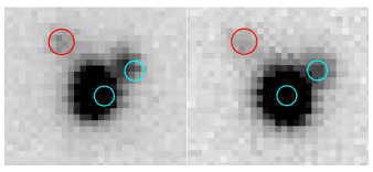
  Figure 11: UGPS $K$-band images for CWISE 0617+1945. (Left) The 2011 Nov image. (Right) The 2013 Apr image. Both images are five arcsec on a side. Circles on both images mark the 2013 positions of CWISE 0617+1945A and CWISE 0617+1945B (cyan) and the non-moving background source (red). North is up and east is to the left.

• 2MASS 0700+3157AB[C]: This system was discovered serendipitously by Thorstensen & Kirkpatrick (2003) when performing astrometric measurements of the unrelated nearby DC10 white dwarf LHS 1889. Using imaging observations with the Hubble Space Telescope, Reid, et al. (2006) discovered a faint companion. Dupuy, & Liu (2017) have performed high-resolution astrometric monitoring of the system and found that the L3: primary is marginally less massive (68.0$\pm$2.6 M_Jup) than the L6.5: secondary ($73.3^{+2.9}_{-3.0}$ M_Jup) despite the large difference in their luminosities. This led those authors to surmise that the B component was comprised of two lower-mass brown dwarfs, although they were unable to find a three-body solution in which theoretical evolutionary models could self consistently apportion the masses and luminosities at a single coeval age. For now, we consider the C component likely, but not confirmed.

• 2MASS 0746+2000AB: Based on its location on the color-magnitude diagram, 2MASS 0746 was suspected to be an unresolved binary by Reid, et al. (2000). Reid et al. (2001b) confirmed this hypothesis with imaging from HST and verified common proper motion of the components using earlier observations from the W. M. Keck Observatory.

• 2MASS 0915+0422AB: This object was discovered by Reid, et al. (2006), who also found it to be a binary using imaging from HST.

• WISE 1049$-$5319AB: This object, commonly referred to as Luhman 16AB, is the third closest system to the Sun and has been known as a binary since its discovery (Luhman 2013).

• Kelu-1AB (1305$-$2541): The overluminosity of this object relative to L dwarfs of similar spectral type had been noted after its trigonometric parallax was measured by Dahn et al. (2002) and Vrba et al. (2004). Liu & Leggett (2005) imaged the companion using the W. M. Keck Observatory and used earlier observations from HST to confirm common proper motion between the components.

• 2MASS 1315$-$2649AB: This highly active L dwarf was discovered serendipitously by Hall (2002) and identified as a binary via high-resolution imaging at the W. M. Keck Observatory by Burgasser et al. (2011b).

• Gl 564BC (1450+2354): Potter, et al. (2002) discovered this close pair as companion binary to the G2 V star Gl 564A using the Gemini North Telescope. Their subsequent observations at Gemini along with spectroscopy from the W. M. Keck Observatory confirmed the physical association of the L dwarf pair with the G dwarf primary.

• 2MASS 1520$-$4422AB: Observations of this object with the New Technology Telescope by Kendall et al. (2007) revealed that the object is a double and that the two components are both L dwarfs. The difference in magnitude between the objects matches expectations if two objects are equidistant.

• 2MASS 1534$-$2952AB: This mid-T dwarf was discovered by Burgasser et al. (2002) and found to be a binary through HST imaging by Burgasser et al. (2003c).

• 2MASS 2152+0937AB: This mid-L dwarf was discovered by Reid, et al. (2006), who also identified it as an equal-magnitude binary through HST imaging.

• Gl 845BC (2204$-$5646): This object is the companion to the nearby K dwarf $\epsilon$ Ind. It was discovered by Scholz et al. (2003) and further identified through imaging as a likely pair of T dwarfs by Volk et al. (2003). McCaughrean et al. (2004) acquired individual spectroscopy to confirm this as a physical pair of T dwarfs.

• DENIS 2252$-$1730AB: Kendall, et al. (2004) discovered this object, and it was identified as a binary system by Reid et al. (2006b) through HST/NICMOS imaging.

• 2MASS 2255$-$5713AB: This object was discovered by Kendall et al. (2007) and identified as a binary system through HST/NICMOS imaging by Reid, et al. (2008b).

Previously suspected multiple systems and new ones identified here for the first time are addressed in section 7.7.

7.4 Analysis of Color-Magnitude and Color-Color Plots

In order to identify other unresolved binaries or subdwarfs in the 20-pc census, we examine color-magnitude and color-color diagrams built from the photometric, astrometric, and spectroscopic data compiled in Table 17. On these we highlight known multiple systems, low-gravity objects, and low-metallicity subdwarfs, as discussed above.

As mentioned in section 5.1.1, the data presented in Table 17 are drawn from a variety of sources, leading to heterogeneity, particularly in the photometric values. For example, although 2MASS covers the entire sky, it is not deep enough to detect many of the late-T and Y dwarfs. For those objects, the hemispheric surveys of UHS in the north and VHS in the south can provide deeper data. Although $H$-band filters are largely invariant across surveys, the same is not true of $J$ and $K$. As shown in Figure 3 of González-Fernández et al. (2018), the 2MASS filters $J_{\rm 2MASS}$ and $K_{S}$ are markedly different from the $J_{\rm MKO}$ and $K_{\rm MKO}$ filters used by WFCAM. Furthermore, although the VISTA employs the same $J_{\rm MKO}$ as WFCAM, its $K_{S}$ filter is much closer to the $K_{S}$ filter used by 2MASS. Similarly, although WISE data in bands W1 and W2 cover the entire sky, deeper observations by Spitzer are done with complementary, though not identical, ch1 and ch2 filters, as shown in Figure 2 of Mainzer et al. (2011).

Ideally, transforming magnitudes in one filter to the complimentary filter in the other survey(s) would allow us to examine homogenized color-color and color-magnitude diagrams using as much data as has been currently collected for the 20-pc L, T, and Y dwarfs. Figure 12 shows the relation in absolute magnitude between $J_{\rm 2MASS}$ and $J_{\rm MKO}$, $K_{S}$ and $K_{\rm MKO}$, W1 and ch1, W2 and ch2. Linear least squares fits to the trends are illustrated in the plots and listed in Table 13. The line of one-to-one correspondence is shown by the black dashed line on each panel.

Figure 12: Plots showing the comparison of absolute magnitudes for objects within the 20-pc census that have measurements in both bands and robust parallax measurements: (a) $M_{J\rm 2MASS}$ vs. $M_{J\rm MKO}$, (b) $M_{Ks\rm 2MASS}$ vs. $M_{K\rm MKO}$, (c) $M_{\rm W1}$ vs. $M_{\rm ch1}$, and (d) $M_{\rm W2}$ vs. $M_{\rm ch2}$. Objects identified as low-gravity, low-metallicity, or having unresolved multiplicity are color coded, per the legend. The brown line shows the linear least-squares fit to the data, excluding color-coded objects. The parameters for these fits are given in Table 13. The one-to-one line is shown by the black dashed line.

The fits to these trends show significant deviations from the one-to-one line for all of these plots except $M_{\rm W2}$ vs. $M_{\rm ch2}$. Transforming between the W2 and ch2 magnitudes is thus an easy transformation (Figure 13; Table 13) not requiring a color or spectral type term. However, transforming between the three other pairs of bands would involve such terms. For these, the uncertainties in the fits as well as uncertainties in the magnitude and color/type measurements would result in a transformed value with a necessarily large uncertainty. Therefore, in the following plots, the only transformations we will include are converting W2 magnitudes into ch2 magnitudes for objects that lack a ch2 measurement.

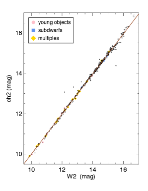
Figure 13: Comparison of the W2 vs. ch2 apparent magnitudes for objects within the 20-pc census that have measurements in both bands. Objects identified as low-gravity, low-metallicity, or having unresolved multiplicity are color coded, per the legend. The brown line shows the linear least-squares fit to the data, excluding color-coded objects. The parameters for this fit are given in Table 13.

Table 13: Polynomial Fits to Trends Shown in Figures 12-20

$x$	$y$	$c_{0}$	$c_{1}$	$c_{2}$	$c_{3}$	$c_{4}$	$c_{5}$	$c_{6}$	$c_{7}$	Valid Range	RMS	Fig#
		($\sigma_{c0}$)	($\sigma_{c1}$)	($\sigma_{c2}$)	($\sigma_{c3}$)	($\sigma_{c4}$)	($\sigma_{c5}$)	($\sigma_{c6}$)	($\sigma_{c7}$)
(1)	(2)	(3)	(4)	(5)	(6)	(7)	(8)	(9)	(10)	(11)	(12)	(13)
$M_{J\rm 2M}$	$M_{J\rm MKO}$	7.0584e-01	9.3542e-01	$\cdots$	$\cdots$	$\cdots$	$\cdots$	$\cdots$	$\cdots$	$10<M_{J\rm 2M}<20$	0.17	12a
		(1.3556e-02)	(9.9161e-04)	$\cdots$	$\cdots$	$\cdots$	$\cdots$	$\cdots$	$\cdots$	$\cdots$	$\cdots$	$\cdots$
$M_{Ks}$	$M_{K\rm MKO}$	-4.5368e-01	1.0358	$\cdots$	$\cdots$	$\cdots$	$\cdots$	$\cdots$	$\cdots$	$9.5<M_{Ks}<18.5$	0.13	12b
		(2.5737e-02)	(2.1127e-03)	$\cdots$	$\cdots$	$\cdots$	$\cdots$	$\cdots$	$\cdots$	$\cdots$	$\cdots$	$\cdots$
$M_{\rm W1}$	$M_{\rm ch1}$	7.8505e-01	8.9844e-01	$\cdots$	$\cdots$	$\cdots$	$\cdots$	$\cdots$	$\cdots$	$9<M_{\rm W1}<20$	0.33	12c
		(1.0156e-02)	(8.1555e-04)	$\cdots$	$\cdots$	$\cdots$	$\cdots$	$\cdots$	$\cdots$	$\cdots$	$\cdots$	$\cdots$
$M_{\rm W2}$	$M_{\rm ch2}$	-9.6870e-02	1.0063	$\cdots$	$\cdots$	$\cdots$	$\cdots$	$\cdots$	$\cdots$	$9<M_{\rm W2}<17$	0.11	12d
		(1.5392e-02)	(1.2866e-03)	$\cdots$	$\cdots$	$\cdots$	$\cdots$	$\cdots$	$\cdots$	$\cdots$	$\cdots$	$\cdots$
W2	ch2	7.0888e-02	9.9268e-01	$\cdots$	$\cdots$	$\cdots$	$\cdots$	$\cdots$	$\cdots$	$9.5<{\rm W2}<17.5$	0.10	13
		(8.9087e-03)	(6.5958e-04)	$\cdots$	$\cdots$	$\cdots$	$\cdots$	$\cdots$	$\cdots$	$\cdots$	$\cdots$	$\cdots$
SpT	$M_{J\rm MKO}$	1.1808e+01	3.3790e-01	-1.9013e-01	7.1759e-02	-9.9829e-03	6.3147e-04	-1.8672e-05	2.1526e-07	$0\leq{\rm SpT}\leq 22$	0.60	14a
		(5.5134e-03)	(8.8293e-03)	(6.1245e-03)	(1.8277e-03)	(2.6582e-04)	(1.9917e-05)	(7.3940e-07)	(1.0762e-08)	$\cdots$	$\cdots$	$\cdots$
SpT	$M_{H}$	1.0966e+01	6.0330e-01	-3.5647e-01	1.1696e-01	-1.6688e-02	1.1719e-03	-4.0259e-05	5.4808e-07	$0\leq{\rm SpT}\leq 22$	0.57	14b
		(1.2196e-02)	(2.0708e-02)	(1.2508e-02)	(3.4795e-03)	(4.9038e-04)	(3.6092e-05)	(1.3227e-06)	(1.9054e-08)	$\cdots$	$\cdots$	$\cdots$
SpT	$M_{\rm ch1}$	9.9434e+00	3.4919e-01	-1.0725e-01	1.7669e-02	-7.1402e-04	-5.0487e-05	4.7761e-06	-9.9981e-08	$0\leq{\rm SpT}\leq 22$	0.38	14c
		(9.9630e-03)	(1.8691e-02)	(1.1499e-02)	(3.1349e-03)	(4.2974e-04)	(3.0823e-05)	(1.1039e-06)	(1.5571e-08)	$\cdots$	$\cdots$	$\cdots$
SpT	$M_{\rm ch2}$	1.0071e+01	1.8897e-01	-6.2186e-02	1.9711e-02	-2.3844e-03	1.3230e-04	-3.3136e-06	2.9971e-08	$0\leq{\rm SpT}\leq 22$	0.31	14d
		(7.3148e-03)	(1.1131e-02)	(7.2528e-03)	(2.1162e-03)	(3.0323e-04)	(2.2351e-05)	(8.1392e-07)	(1.1594e-08)	$\cdots$	$\cdots$	$\cdots$
SpT	$J-{\rm ch2}$	1.8153e+00	1.8527e-01	-1.7678e-01	7.2989e-02	-1.1351e-02	8.1335e-04	-2.7663e-05	3.6779e-07	$0\leq{\rm SpT}\leq 22$	0.44	14e
		(7.9722e-03)	(1.1627e-02)	(7.0547e-03)	(1.9164e-03)	(2.6068e-04)	(1.8578e-05)	(6.6362e-07)	(9.3747e-09)	$\cdots$	$\cdots$	$\cdots$
SpT	$H-{\rm ch2}$	1.1150e+00	6.7204e-02	-7.3996e-02	4.0283e-02	-7.1625e-03	5.7419e-04	-2.1740e-05	3.2110e-07	$0\leq{\rm SpT}\leq 22$	0.42	14f
		(1.5068e-02)	(2.3813e-02)	(1.3338e-02)	(3.4641e-03)	(4.6215e-04)	(3.2659e-05)	(1.1624e-06)	(1.6400e-08)	$\cdots$	$\cdots$	$\cdots$
SpT	ch1 $-$ ch2	2.6662e-02	-2.6015e-02	8.1897e-04	3.2520e-04	$\cdots$	$\cdots$	$\cdots$	$\cdots$	$0\leq{\rm SpT}\leq 22$	0.19	14g
		(8.2684e-03)	(3.1254e-03)	(3.3481e-04)	(1.0531e-05)	$\cdots$	$\cdots$	$\cdots$	$\cdots$	$\cdots$	$\cdots$	$\cdots$
SpT	W1 $-$ W2	2.2668e-01	2.9069e-02	-4.6379e-03	5.7825e-04	$\cdots$	$\cdots$	$\cdots$	$\cdots$	$0\leq{\rm SpT}\leq 22$	0.28	14h
		(4.6612e-03)	(2.0308e-03)	(2.5436e-04)	(9.1089e-06)	$\cdots$	$\cdots$	$\cdots$	$\cdots$	$\cdots$	$\cdots$	$\cdots$
$M_{J\rm MKO}$	SpT	-7.7784e+01	1.3260e+01	-6.1185e-01	9.6221e-03	$\cdots$	$\cdots$	$\cdots$	$\cdots$	$14.3\leq M_{J\rm MKO}\leq 24.0$	0.53	15a
		(1.5730e+01)	(2.6086e+00)	(1.4247e-01)	(2.5610e-03)	$\cdots$	$\cdots$	$\cdots$	$\cdots$	$\cdots$	$\cdots$	$\cdots$
$M_{H}$	SpT	-6.9184e+01	1.1863e+01	-5.4084e-01	8.4661e-03	$\cdots$	$\cdots$	$\cdots$	$\cdots$	$14.5\leq M_{H}\leq 24.0$	0.51	15b
		(1.5192e+01)	(2.5100e+00)	(1.3661e-01)	(2.4473e-03)	$\cdots$	$\cdots$	$\cdots$	$\cdots$	$\cdots$	$\cdots$	$\cdots$
$M_{\rm ch1}$	SpT	-1.2682e+02	2.1824e+01	-1.0888e+00	1.8362e-02	$\cdots$	$\cdots$	$\cdots$	$\cdots$	$10.0\leq M_{\rm ch1}\leq 19.0$	0.89	15c
		(1.3047e+01)	(2.8362e+00)	(2.0216e-01)	(4.7350e-03)	$\cdots$	$\cdots$	$\cdots$	$\cdots$	$\cdots$	$\cdots$	$\cdots$
$M_{\rm ch2}$	SpT	1.4559e+03	-4.6516e+02	5.4301e+01	-2.7423e+00	5.0950e-02	$\cdots$	$\cdots$	$\cdots$	$10.0\leq M_{\rm ch2}\leq 16.0$	1.26	15d
		(3.8543e+02)	(1.2245e+02)	(1.4499e+01)	(7.5845e-01)	(1.4790e-02)	$\cdots$	$\cdots$	$\cdots$	$\cdots$	$\cdots$	$\cdots$
$J-{\rm ch2}$	SpT	1.1022e+01	3.4335e+00	-4.8308e-01	2.6036e-02	$\cdots$	$\cdots$	$\cdots$	$\cdots$	$2.1\leq J-{\rm ch2}\leq 8.5$	0.53	15e
		(6.2228e-01)	(4.6900e-01)	(1.0643e-01)	(7.2766e-03)	$\cdots$	$\cdots$	$\cdots$	$\cdots$	$\cdots$	$\cdots$	$\cdots$
$H-{\rm ch2}$	SpT	1.0280e+01	3.5828e+00	-5.0032e-01	2.7292e-02	$\cdots$	$\cdots$	$\cdots$	$\cdots$	$2.4\leq H-{\rm ch2}\leq 8.3$	0.54	15f
		(8.4671e-01)	(6.1648e-01)	(1.3683e-01)	(9.2515e-03)	$\cdots$	$\cdots$	$\cdots$	$\cdots$	$\cdots$	$\cdots$	$\cdots$
ch1 $-$ ch2	SpT	5.4614e+00	2.1717e+01	-1.6691e+01	6.1763e+00	-8.1737e-01	$\cdots$	$\cdots$	$\cdots$	$0.1\leq{\rm ch1}-{\rm ch2}\leq 3.0$	1.26	15g
		(1.5994e-01)	(1.0797e+00)	(1.7084e+00)	(8.9977e-01)	(1.5127e-01)	$\cdots$	$\cdots$	$\cdots$	$\cdots$	$\cdots$	$\cdots$
W1 $-$ W2	SpT	-3.9840e+00	3.4029e+01	-2.5352e+01	1.0073e+01	-1.9779e+00	1.5181e-01	$\cdots$	$\cdots$	$0.4\leq{\rm W1}-{\rm W2}\leq 4.0$	1.16	15h
		(5.8726e-01)	(2.7025e+00)	(3.8349e+00)	(2.3059e+00)	(6.1348e-01)	(5.9415e-02)	$\cdots$	$\cdots$	$\cdots$	$\cdots$	$\cdots$
ch1 $-$ ch2	$M_{J\rm MKO}$	1.4839e+01	-1.5369e+00	1.3741e+00	4.7706e-02	$\cdots$	$\cdots$	$\cdots$	$\cdots$	$0.2\leq{\rm ch1}-{\rm ch2}\leq 3.7$	0.82	16a
		(1.9346e-02)	(4.9810e-02)	(3.7680e-02)	(8.4926e-03)	$\cdots$	$\cdots$	$\cdots$	$\cdots$	$\cdots$	$\cdots$	$\cdots$
ch1 $-$ ch2	$M_{H}$	1.3650e+01	4.2277e-01	5.9475e-01	1.4662e-01	$\cdots$	$\cdots$	$\cdots$	$\cdots$	$0.2\leq{\rm ch1}-{\rm ch2}\leq 3.7$	0.73	16b
		(2.9219e-02)	(7.3179e-02)	(5.4990e-02)	(1.2372e-02)	$\cdots$	$\cdots$	$\cdots$	$\cdots$	$\cdots$	$\cdots$	$\cdots$
ch1 $-$ ch2	$M_{\rm ch2}$	1.1685e+01	1.2405e+00	-2.6707e-01	9.7851e-02	$\cdots$	$\cdots$	$\cdots$	$\cdots$	$0.2\leq{\rm ch1}-{\rm ch2}\leq 3.7$	0.37	16c
		(2.1383e-02)	(4.3465e-02)	(2.6277e-02)	(4.6742e-03)	$\cdots$	$\cdots$	$\cdots$	$\cdots$	$\cdots$	$\cdots$	$\cdots$
ch1 $-$ ch2	$J-{\rm ch2}$	3.2442e+00	-3.3515e+00	2.2401e+00	-2.1036e-01	$\cdots$	$\cdots$	$\cdots$	$\cdots$	$0.4\leq{\rm ch1}-{\rm ch2}\leq 3.7$	0.59	16d
		(1.0321e-02)	(2.9530e-02)	(2.4059e-02)	(5.7791e-03)	$\cdots$	$\cdots$	$\cdots$	$\cdots$	$\cdots$	$\cdots$	$\cdots$
ch1 $-$ ch2	$H-{\rm ch2}$	1.8968e+00	-3.8478e-01	5.4798e-01	1.0067e-01	$\cdots$	$\cdots$	$\cdots$	$\cdots$	$0.4\leq{\rm ch1}-{\rm ch2}\leq 3.7$	0.54	16e
		(1.5548e-02)	(4.6766e-02)	(3.8685e-02)	(9.2812e-03)	$\cdots$	$\cdots$	$\cdots$	$\cdots$	$\cdots$	$\cdots$	$\cdots$
ch1 $-$ ch2	W1 $-$ W2	3.6295e-01	1.4472e+00	-9.0895e-02	$\cdots$	$\cdots$	$\cdots$	$\cdots$	$\cdots$	$0.0\leq{\rm ch1}-{\rm ch2}\leq 3.7$	0.26	16f
		(1.7547e-03)	(6.3917e-03)	(3.7513e-03)	$\cdots$	$\cdots$	$\cdots$	$\cdots$	$\cdots$	$\cdots$	$\cdots$	$\cdots$
W1 $-$ W2	$M_{J\rm MKO}$	1.5375e+01	-1.8851e+00	8.6518e-01	$\cdots$	$\cdots$	$\cdots$	$\cdots$	$\cdots$	$1.0\leq{\rm W1}-{\rm W2}\leq 4.5$	1.06	17a
		(3.0925e-02)	(2.6582e-02)	(5.4656e-03)	$\cdots$	$\cdots$	$\cdots$	$\cdots$	$\cdots$	$\cdots$	$\cdots$	$\cdots$
W1 $-$ W2	$M_{H}$	1.3974e+01	-5.0420e-01	6.1351e-01	$\cdots$	$\cdots$	$\cdots$	$\cdots$	$\cdots$	$1.0\leq{\rm W1}-{\rm W2}\leq 4.5$	0.97	17b
		(5.0500e-02)	(4.2061e-02)	(8.3712e-03)	$\cdots$	$\cdots$	$\cdots$	$\cdots$	$\cdots$	$\cdots$	$\cdots$	$\cdots$
W1 $-$ W2	$M_{\rm ch2}$	1.1923e+01	3.2350e-01	1.1564e-01	$\cdots$	$\cdots$	$\cdots$	$\cdots$	$\cdots$	$1.0\leq{\rm W1}-{\rm W2}\leq 4.5$	0.46	17c
		(4.6335e-02)	(3.6466e-02)	(6.8309e-03)	$\cdots$	$\cdots$	$\cdots$	$\cdots$	$\cdots$	$\cdots$	$\cdots$	$\cdots$
W1 $-$ W2	$J-{\rm W2}$	3.4006e+00	-2.0109e+00	6.8777e-01	$\cdots$	$\cdots$	$\cdots$	$\cdots$	$\cdots$	$1.0\leq{\rm W1}-{\rm W2}\leq 4.5$	0.77	17e
		(1.1512e-02)	(1.1197e-02)	(2.5620e-03)	$\cdots$	$\cdots$	$\cdots$	$\cdots$	$\cdots$	$\cdots$	$\cdots$	$\cdots$
W1 $-$ W2	$H-{\rm W2}$	1.0705e+00	8.5334e-01	-3.0341e-01	1.1371e-01	$\cdots$	$\cdots$	$\cdots$	$\cdots$	$1.0\leq{\rm W1}-{\rm W2}\leq 4.5$	0.67	17f
		(4.6358e-02)	(6.8836e-02)	(3.2019e-02)	(4.6830e-03)	$\cdots$	$\cdots$	$\cdots$	$\cdots$	$\cdots$	$\cdots$	$\cdots$
$J_{\rm MKO}-{\rm ch2}$	$M_{J\rm MKO}$	1.1915e+01	1.5841e+00	-1.6137e-02	$\cdots$	$\cdots$	$\cdots$	$\cdots$	$\cdots$	$1.0\leq J_{\rm MKO}-{\rm ch2}\leq 12.0$	0.39	18a
		(4.9157e-02)	(2.3193e-02)	(2.4580e-03)	$\cdots$	$\cdots$	$\cdots$	$\cdots$	$\cdots$	$\cdots$	$\cdots$	$\cdots$
$J_{\rm MKO}-{\rm ch2}$	$M_{H}$	1.1583e+01	1.9032e+00	-5.0925e-02	$\cdots$	$\cdots$	$\cdots$	$\cdots$	$\cdots$	$1.0\leq J_{\rm MKO}-{\rm ch2}\leq 12.0$	0.42	18b
		(3.3133e-02)	(1.7627e-02)	(2.0930e-03)	$\cdots$	$\cdots$	$\cdots$	$\cdots$	$\cdots$	$\cdots$	$\cdots$	$\cdots$
$J_{\rm MKO}-{\rm ch2}$	$M_{\rm ch2}$	1.2404e+01	3.6423e-01	4.5527e-03	$\cdots$	$\cdots$	$\cdots$	$\cdots$	$\cdots$	$1.0\leq J_{\rm MKO}-{\rm ch2}\leq 12.0$	0.34	18c
		(1.9595e-02)	(7.9067e-03)	(6.5360e-04)	$\cdots$	$\cdots$	$\cdots$	$\cdots$	$\cdots$	$\cdots$	$\cdots$	$\cdots$
$H-{\rm ch2}$	$M_{J\rm MKO}$	1.1777e+01	1.4108e+00	-4.6998e-05	$\cdots$	$\cdots$	$\cdots$	$\cdots$	$\cdots$	$2.5\leq H-{\rm ch2}\leq 12.0$	0.50	19a
		(5.9763e-02)	(2.5921e-02)	(2.5617e-03)	$\cdots$	$\cdots$	$\cdots$	$\cdots$	$\cdots$	$\cdots$	$\cdots$	$\cdots$
$H-{\rm ch2}$	$M_{H}$	1.1454e+01	1.6462e+00	-1.7633e-02	$\cdots$	$\cdots$	$\cdots$	$\cdots$	$\cdots$	$2.0\leq H-{\rm ch2}\leq 12.0$	0.35	19b
		(4.2250e-02)	(2.0841e-02)	(2.3369e-03)	$\cdots$	$\cdots$	$\cdots$	$\cdots$	$\cdots$	$\cdots$	$\cdots$	$\cdots$
$H-{\rm ch2}$	$M_{\rm ch2}$	1.2709e+01	1.4789e-01	2.7211e-02	$\cdots$	$\cdots$	$\cdots$	$\cdots$	$\cdots$	$3.0\leq H-{\rm ch2}\leq 12.0$	0.30	19c
		(2.6042e-02)	(1.0488e-02)	(9.1350e-04)	$\cdots$	$\cdots$	$\cdots$	$\cdots$	$\cdots$	$\cdots$	$\cdots$	$\cdots$
$M_{H}$	$T_{\rm eff}$	1.2516e+04	-1.5666e+03	6.7502e+01	-9.2430e-01	-1.9530e-03	$\cdots$	$\cdots$	$\cdots$	$9.5\leq M_{H}\leq 25.0$	88.1	20a
		(1.0770e+03)	(2.7058e+02)	(2.4638e+01)	(9.6594e-01)	(1.3793e-02)	$\cdots$	$\cdots$	$\cdots$	$\cdots$	$\cdots$	$\cdots$
SpT	$T_{\rm eff}$	2.2375e+03	-1.4496e+02	4.0301e+00	$\cdots$	$\cdots$	$\cdots$	$\cdots$	$\cdots$	$0.0\leq SpT\leq 8.75$	134	20b
		(1.1342e+01)	(4.2745e+00)	(8.8587e-01)	$\cdots$	$\cdots$	$\cdots$	$\cdots$	$\cdots$	$\cdots$	$\cdots$	$\cdots$
SpT	$T_{\rm eff}$	1.4379e+03	-1.8309e+01	$\cdots$	$\cdots$	$\cdots$	$\cdots$	$\cdots$	$\cdots$	$8.75\leq SpT\leq 14.75$	79	20b
SpT	$T_{\rm eff}$	5.1413e+03	-3.6865e+02	6.7301e+00	$\cdots$	$\cdots$	$\cdots$	$\cdots$	$\cdots$	$14.75\leq SpT\leq 22.0$	79	20b
		(7.9271e+02)	(8.7788e+01)	(2.4174e+00)	$\cdots$	$\cdots$	$\cdots$	$\cdots$	$\cdots$	$\cdots$	$\cdots$	$\cdots$

Note. — These are simple polynomial equations of the form

$$y=\sum_{i=0}^{n}c_{i}x^{i}.$$

For spectral types, SpT = 0 for L0, SpT = 5 for L5, SpT = 10 for T0, SpT = 15 for T5, SpT = 20 for Y0, etc.

Trends of absolute magnitude with spectral type are illustrated in Figure 14(a-d). Most of the known, unresolved doubles have components of nearly equal magnitudes, and not surprisingly, most of these objects stand out as overluminous for their types relative to the main trends. On the plots of $M_{J\rm MKO}$ and $M_{H}$, T-type subdwarfs tend to be overluminous with respect to the mean trend, whereas L-type subdwarfs are underluminous, although for the latter there are only two examples with which to judge. At $M_{\rm ch1}$ and $M_{\rm ch2}$, the subdwarfs are indistiguishable from objects of solar metallicity. Young L dwarfs within 20 pc tend to be overluminous with respect to the mean trend in all four absolute magnitudes, whereas young T dwarfs – at least for the three known examples – do not distinguish themselves from the run of older T dwarfs.

Trends of colors with spectral type are illustrated in Figure 14(e-h). The two known L subdwarfs are much bluer than the mean trend in $J_{\rm MKO}-{\rm ch2}$ and $H-{\rm ch2}$ colors, though indistinguishable from the mean trend in ${\rm ch1}-{\rm ch2}$ and ${\rm W1}-{\rm W2}$. The T subdwarfs tend to lie redward of the mean trend in all four colors. Young L dwarfs are markedly redder than the trend in all four colors, whereas the few young T dwarfs known do not clearly differentiate themselves.

Figure 14: Plots of various absolute magnitudes (a-d) and colors (e-h) as a function of near-infrared spectral type. Only members of the 20-pc census are shown, and plots a-d show only the subset of 20-pc objects having parallaxes measured to better than 12.5%. Plots of $M_{\rm ch2}$, $J_{\rm MKO}-{\rm ch2}$, and $H-{\rm ch2}$ are supplemented with W2 magnitudes when ch2 magnitudes are not available, as described in section 7.4. Polynomial fits that exclude known young objects (pink circles, section 7.1), subdwarfs (blue squares, section 7.2), and multiple systems (yellow diamonds, section 7.3) are shown in brown and described in Table 13.

In Figure 15(a-h), we show these same plots as above, but with the axes flipped. This is to provide researchers with fits to convert absolute magnitudes or colors to a spectral type. As is illustrated in the plots, it is not always possible to provide simple polynomial fits over the entire range of absolute magnitude or color because of degeneracies. For example, a color of $J_{\rm MKO}-{\rm ch2}=3.0$ mag corresponds to either a mid/late-L dwarf or a mid/late-T dwarf. Users are urged to check the notes in Table 13 to check the ranges over which these fits are valid.

Figure 15: Plots identical to those of Figure 14, except that the $x$ and $y$ axes have been reversed. Polynomial fits to provide a translation from absolute magnitude or color into spectral type are shown in brown and described in Table 13. These fits exclude known young objects (pink circles, section 7.1), subdwarfs (blue squares, section 7.2), and multiple systems (yellow diamonds, section 7.3).

In Figure 16(a-f), we illustrate trends of absolute magnitudes and colors as a function of ${\rm ch1}-{\rm ch2}$ color. In the plots of absolute magnitude, multiples are seen as overluminous, as expected, and only the most metal poor T subdwarf, WISE 2005+5424 ([Fe/H] = $-0.64{\pm}0.17$) is well removed from the trend in $M_{J\rm MKO}$ and $M_{H}$. On the color plots, the T subdwarfs are redder in $J_{\rm MKO}-{\rm ch2}$, $H-{\rm ch2}$, and ${\rm W1}-{\rm W2}$ at a fixed value of ${\rm ch1}-{\rm ch2}$.

Figure 16: Plots of various absolute magnitudes (a-c) and colors (d-f) as a function of ${\rm ch1}-{\rm ch2}$ color. Only members of the 20-pc census are shown, and plots a-c show only the subset of 20-pc objects having parallaxes measured to better than 12.5%. Polynomial fits that exclude known young objects (pink circles, section 7.1), subdwarfs (blue squares, section 7.2), and multiple systems (yellow diamonds, section 7.3) are shown in brown and described in Table 13. Fits include only those points with ${\rm ch1}-{\rm ch2}>0.2$ mag for panels a-e.

Plots of absolute magnitude and color as a function of ${\rm W1}-{\rm W2}$ color are shown in Figure 17(a-f). The same trends as those mentioned above in ${\rm ch1}-{\rm ch2}$ color are seen.

Figure 17: Plots of various absolute magnitudes (a-c) and colors (d-f) as a function of ${\rm W1}-{\rm W2}$ color. Only members of the 20-pc census are shown, and plots a-c show only the subset of 20-pc objects having parallaxes measured to better than 12.5%. Polynomial fits that exclude known young objects (pink circles, section 7.1), subdwarfs (blue squares, section 7.2), and multiple systems (yellow diamonds, section 7.3) are shown in brown and described in Table 13. In panels a-c, the fits include only those points with ${\rm W1}-{\rm W2}>1.0$ mag, and in panels e-f the fits include only those points with ${\rm W1}-{\rm W2}>0.8$ mag

Plots of absolute magnitude and color as a function of $J_{\rm MKO}-{\rm ch2}$ and $H-{\rm ch2}$ color are shown in Figure 18(a-e) and Figure 19(a-e). At a given absolute magnitude in $M_{J\rm MKO}$, $M_{H}$, and $M_{\rm ch2}$, young L dwarfs are shown to be redder than field objects, as are T subdwarfs, although L subdwarfs appear bluer. On the color-color plots, the reddest of the young L dwarfs are the reddest objects of all in $J_{\rm MKO}-K_{\rm MKO}$; at their ${\rm W1}-{\rm W2}$ colors, they are also the reddest objects in $J_{\rm MKO}-{\rm ch2}$ and $H-{\rm ch2}$.

Figure 18: Plots of various absolute magnitudes (a-c) and colors (d-e) as a function of $J_{\rm MKO}-{\rm ch2}$ color. Only members of the 20-pc census are shown, and plots a-c show only the subset of 20-pc objects having parallaxes measured to better than 12.5%. All five panels are supplemented with W2 magnitudes when ch2 is not available, as described in section 7.4. Polynomial fits that exclude known young objects (pink circles, section 7.1), subdwarfs (blue squares, section 7.2), and multiple systems (yellow diamonds, section 7.3) are shown in brown and described in Table 13. These fits are restricted to points with $M_{J\rm MKO}\geq 16.0$ mag in panel a, $M_{H}\geq 15.0$ mag in panel b, and $M_{\rm ch2}\geq 13.0$ mag in panel c.

Figure 19: Plots of various absolute magnitudes (a-c) and colors (d-e) as a function of $H-{\rm ch2}$ color. Only members of the 20-pc census are shown, and plots a-c show only the subset of 20-pc objects having parallaxes measured to better than 12.5%. All five panels are supplemented with W2 magnitudes when ch2 is not available, as described in section 7.4. Polynomial fits that exclude known young objects (pink circles, section 7.1), subdwarfs (blue squares, section 7.2), and multiple systems (yellow diamonds, section 7.3) are shown in brown and described in Table 13. These fits are restricted to points with $M_{J\rm MKO}\geq 16.0$ mag in panel a, $M_{H}\geq 15.0$ mag in panel b, and $M_{\rm ch2}\geq 13.0$ mag in panel c.

Having established the locations of unusual objects on these diagrams, we examine the evidence for other, previously unrecognized (or, in some cases, previously suspected) young dwarfs, subdwarfs, and multiples in the 20-pc census. These are discussed in the next three subsections.

7.5 Potential Young Objects

No newly recognized young object candidates were identified from these diagrams.

7.6 Potential Subdwarfs

A number of objects, not discussed in section 7.2 above, appear to fall along the subdwarf locus in Figures 14 through 19. These are addressed below.

• WISE 0316+4307: This T8 dwarf falls along the locus of subdwarfs in the color-type plots shown in Figures 14e and f. It also appears as a color outlier on the color-color plot 17f. Mace et al. (2013) acquired separate $J$- and $H$-band spectra of the object and did not note any peculiarities, although a spectrum across the full $JHK$ wavelength range could elucidate whether the telltale $K$-band suppression seen in T subdwarfs is confirmed.

• WISE 0359$-$5401: This Y0 dwarf falls along the locus of subdwarfs in Figure 16d. No Y dwarfs have yet been classified as subdwarfs, but Leggett et al. (2017) found this object indeed falls in the part of the $J-{\rm ch2}$ vs. ${\rm ch1}-{\rm ch2}$ diagram where substellar models predict low-metallicity objects to fall. We consider this to be a normal Y dwarf in subsequent analysis, pending the empirical spectroscopic identification of other Y subdwarfs.

• WISE 0430+4633: This T8 dwarf falls along the locus of subdwarfs in the color-type plots of Figures 14e and f. It is also a color outlier on the color-type plot of Figure 14h and the color-color plot of Figure 16f. The spectral classification of this object is based on only a $J$-band spectrum by Mace et al. (2013). As with WISE 0316+4307 above, a spectrum across the full $JHK$ wavelength range is needed to confirm whether a subdwarf classification is warranted.

• UGPS 0521+3640: This T8.5 dwarf falls along the subdwarf locus in the absolute magnitude-color plot of Figure 16b. It is also an outlier on the color-color plot of Figure 16f. However, this source’s photometry may be confused by the halo of a much brighter star. The near-infrared spectrum by Burningham et al. (2011) shows no peculiarities, so we think it is only the poor photometry that is causing this object to appear as an outlier.

• WISE 0751$-$7634: This T9 dwarf falls along the subdwarf locus in the absolute magnitude-color plots of Figures 16a,b and 17a,b, as well as in the color-color plot of Figure 17e. It is also an outlier on the color-color plot of Figure 17f. The near-infrared spectrum shown by Kirkpatrick et al. (2011) has low S/N in the $K$-band and may show the flux suppression typical of T subdwarfs, but an improved spectrum is needed to verify this. Leggett et al. (2017) notes that this object falls within the locus on the $J-{\rm ch2}$ vs. ${\rm ch1}-{\rm ch2}$ diagram where substellar models predict low-metallicity objects to fall. We await improved spectroscopic data before classifying this object as a subdwarf.

• WISE 1112$-$3857: This T9 dwarf falls along the subdwarf locus in the color-type plots of Figures 14e,f, and the color-color plot of Figure 16d. The near-infrared spectrum presented in Tinney et al. (2018) does not extend to the $K$-band but appears to show excess flux on the blueward side of $Y$-band, as seen in other T subdwarfs (see section 7.2). A more complete spectrum at higher S/N is needed to confirm the subdwarf hypothesis.

• WISE 1141$-$3326: This is a Y0 dwarf that falls along the subdwarf locus in the absolute magnitude-color plots of Figures 16a and 17a, and the color-color plots of Figure 16d and 17e. As noted in Kirkpatrick et al. (2019), however, these anomalies can likely be attributed to photometric contamination at earlier epochs when the source was passing in front of a background galaxy.

• WISE 1818$-$4701: A spectrum of this object has not yet been acquired, but it is believed to be a late-T dwarf. It falls along the subdwarf locus in the absolute magnitude-color plot of Figure 17a and color-color plot of Figure 17e. A spectrum is required to confirm or refute the subdwarf hypothesis.

• GJ 836.7B (2144+1446): This T3 dwarf, also known as HN Peg B, appears along the subdwarf sequence in the color-color plot of Figure 17f and is an outlier on the color-type plot of Figure 14h and the color-color plot of Figure 16f. Luhman et al. (2007) cite an age of $\sim$300 Myr for the system, and Valenti & Fischer (2005) find that the primary has [M/H] $\approx-0.01$. Since this object is obviously not a subdwarf, we suspect that the CatWISE2020 photometry may be corrupted due to the proximity of the bright primary itself. The AllWISE and CatWISE2020 photometry (Table 17) differ in both W1 and W2 by $>5{\sigma}$, indicating that the the automated measurements are likely poor. Further evidence that the ${\rm W1}-{\rm W2}$ color may be suspect is the fact that similar plots with ${\rm ch1}-{\rm ch2}$ color (Figures 14g and 16e) show this source falling along the locus of normal field dwarfs.

• GJ 1263B (2146$-$0010): This T8.5 dwarf, also known as Wolf 940B, lies along the subdwarf locus in Figures 17a,b. Burningham et al. (2009) find that the primary has an age of $\sim$3.5 Gyr and metallicity of [Fe/H] $=-0.06{\pm}0.20$, so the B component cannot be a subdwarf. As with GJ 836.7B above, the AllWISE and CatWISE2020 photometry (Table 17) differ in both W1 and W2, in this case by $>10{\sigma}$ and $>6{\sigma}$, respectively. Further evidence that the ${\rm W1}-{\rm W2}$ color may be suspect is the fact that similar plots with ${\rm ch1}-{\rm ch2}$ color (Figures 16a,b) show this source to fall along the normal locus. We suspect that the bright primary has corrupted the WISE photometry of the secondary.

7.7 Potential Multiples

Several L, T and Y dwarfs within the 20-pc census have been previously published as suspected multiples and either remain unconfirmed or have subsequently been discounted. Several others are newly addressed here as suspected binary systems. Suspected companions are denoted by brackets ("[B]" or "[C]") around the suffix both in the text below and in Table 11.

• WISE 0309$-$5016A[B]: This T7 dwarf is an outlier on the absolute magnitude-type plot of Figure 14d and on the absolute magnitude-color plots of Figure 16b,c; 17a,b,c; 18a,b,c; and 19a,b,c. The consistent overluminosity of this object across colors and bands strongly points to its being an unresolved double with components of near-equal magnitude. As we did in Kirkpatrick et al. (2019), we consider it to be a two-body system in subsequent analysis.

• WISE 0350$-$5658: This Y1 dwarf falls well above the mean trend in Figure 16b. Oddities in absolute magnitude-type plots were also noted in Kirkpatrick et al. (2019). Few Y1 dwarfs are presently known, so it is unclear the extent to which this is just cosmic scatter for normal dwarfs of this spectral type. We consider this object to be single.

• WISE 0535$-$7500: This $\geq$Y1: dwarf falls well above the mean trend on the absolute magnitude-type plot of Figure 14d and on the absolute magnitude-color plots of Figures 16c; 18a,c; and 19a,b,c. This overluminosity was also noted by Tinney et al. (2014), Leggett et al. (2017), and Kirkpatrick et al. (2019). Opitz et al. (2016) used adaptive-optics imaging to rule any equal-magnitude companion at a separation greater than $\sim$1.9 AU. As with WISE 0350$-$5658 above, it is unclear the extent to which this may just be cosmic scatter for normal dwarfs of this spectral type, since few are known. We consider this object to be single.

• WISE 0546$-$0959: This T5 dwarf falls above the mean locus on the $M_{H}$ vs. ${\rm ch1}-{\rm ch2}$ diagram of Figure 16b and the $M_{H}$ vs. ${\rm W1}-{\rm W2}$ diagram of Figure 17b. Because it appears overluminous only in $H$-band, we consider this object to be single.

• 2MASS 0559$-$1404: This mid-T dwarf falls well above the mean locus on all of the plots based on absolute magnitude in Figures 14, 16, and 17. It is also an outlier on the $M_{J\rm MKO}$ vs. $J_{\rm MKO}-{\rm ch2}$ plot of Figure 18a. Two hypotheses have been proposed to explain the overluminosity, which was first noted by Dahn et al. (2002): (1) Burgasser (2001) suggested that the object was an equal-magnitude binary. (2) Burgasser et al. (2003c) later proposed that the quick dissipation of clouds near the L-to-T dwarf transition could be responsible for the overluminosity, which is largest at $J$-band. However, both of these hypotheses have encountered problems in the intervening years. The cloud disruption theory was largely invoked to explain the $J$-band overluminosity (Tsuji & Nakajima 2003), but as our figures show, this overluminosity is present across all bands from $J$ through W2. The binary theory has yet to be confirmed, either. High-resolution HST imaging by Burgasser et al. (2003c) showed no indication of a hidden companion down to a separation of 0$\farcs$09. Using radial velocity measurements covering a 4.4-yr period, Zapatero Osorio et al. (2007) found no velocity variations (to $1\sigma=0.5$ km s^-1). Other radial velocity measurements by Prato et al. (2015) were able to rule out a companion with a period of a day or less, but these authors stress that there is still orbital parameter space between their sampled region and the 0$\farcs$09 (0.9 AU) limit by the HST imaging mentioned above. Given the inability of observers to confirm the binary hypothesis for this object, we will assume the object is a single dwarf in subsequent analysis.

• PSO 0652+4127: Best et al. (2013) label this object as a possible binary based on the fact that some near-infrared spectral indices better match a L8+T2.5 composite that the single T0 type. Their single-object photometric distance suggests the object falls at 14.2$\pm$1.2 pc, whereas the binary hypothesis suggests 20.1$\pm$2.4 pc. Our Spitzer parallax gives a distance of 17.4$\pm$1.0 pc, which is intermediate between the two estimates. In the absence of data confirming a companion, we consider this object to be single.

• SDSS 0758+3247: This early T dwarf was discovered by Knapp et al. (2004). It was identified by Burgasser et al. (2010) as a weak candidate for unresolved binarity due to its near-infrared spectral morphology. However, as stated in that paper, the single object spectral fit outperformed that of the best binary fit. Nonetheless, the spectral type listed in the SIMBAD database shows this as a composite type. Bardalez Gagliuffi et al. (2015) list this system as a "visual spectral binary" but surmise that it is comprised of two components with types of T2.2$\pm$0.0 and T2.3$\pm$0.0 despite the fact that it is not possible to detect a binary comprised of identical components using low-resolution spectral morphology alone. Our plot of M_H vs. near-infrared spectral type, for example, shows no overluminosity of this object compared to other early-T dwarfs, ruling out the equal-magnitude binary hypothesis. We thus consider this object to be a single brown dwarf.

• SDSS 0857+5708: This L8 dwarf falls above the mean trend on the plots of $M_{\rm ch1}$ and $M_{\rm ch2}$ vs. spectral type in Figures 14c,d. Given that there is no evidence of overluminosity in other diagrams and that there is no indication in the literature of binarity, we consider this to be a single object.

• WISE 0920+4538: Given that this L9 dwarf is labeled only as a weak binary candidate in Mace et al. (2013) and that some of its peculiarities may be attributed to spectroscopic variations (Best et al. 2013), we consider this to be a single object.

• 2MASS 0939$-$2448A[B]: This T8 dwarf has been considered an unresolved, equal-magnitude binary for many years based on its overluminosity, as discussed in Kirkpatrick et al. (2019). In section 7.2, we noted that the spectrum shows signs of low-metallicity as well. Thus, we consider this to be a T subdwarf binary.

• PSO 0956$-$1447: Best et al. (2015) list this late-L dwarf as a marginal spectral binary candidate. In the absence of any confirming high-resolution imaging, we consider this to be a single object.

• SDSS 1048+0111: This early- to mid-L dwarf falls above the mean locus on the plots of absolute magnitude vs. spectral type in Figures 14a,b. Reid, et al. (2006) did not find any evidence of binarity in high-resolution HST imaging. Furthermore, we note that our perceived overluminosity vanishes if we plot against the optical spectral type of L1 instead of the near-infrared type of L4 (Table 11). We consider this to be a single object.

• 2MASS 1231+0847: This T5.5 dwarf is overluminous for its ${\rm ch1}-{\rm ch2}$ and ${\rm W1}-{\rm W2}$ color on Figures 16a,b,c and 17a,b,c. The object was observed with high-resolution imaging on HST by Aberasturi et al. (2014), who found no companion with a separation $>0{\farcs}3$ down to $\Delta{J}\approx 2.5$ mag (their Figure 7). As discussed in Kirkpatrick et al. (2019), Burgasser et al. (2004) proposed that this object’s broad K I lines might indicate a higher gravity that is the consequence of lower metallicity. Given the uncertain cause of this object’s peculiarities, we will consider it to be a single dwarf of normal metallicity in subsequent analysis.

• WISE 1318$-$1758: This T8 dwarf is overluminous on the $M_{H}$ vs. ${\rm ch1}-{\rm ch2}$ plot of Figure 16b and the $M_{H}$ vs. $J_{\rm MKO}-{\rm ch2}$ plot of Figure 18b. Because the object does not appear overluminous on other plots, we consider it to be single.

• WISE 1322$-$2340: This late-T dwarf is overluminous only on the $M_{H}$ vs. ${\rm ch1}-{\rm ch2}$ plot of Figure 16b although Kirkpatrick et al. (2019) noted it was an outlier in $H-{\rm ch2}$ color as well. However, the object does not distinguish itself on other plots, and Gelino et al. (2011) ruled out any companion with a separation $>0{\farcs}2$ down to $\Delta{H}\approx 4.0$ mag. We consider this object to be single.

• ULAS 1416+1348: In Kirkpatrick et al. (2019), we considered this (sd)T7.5 to be an unresolved double based on its overluminosity with respect to normal late-T dwarfs and with respect to the few sdT dwarfs identified in that paper. However, it now appears that overluminosity with respect to normal T dwarfs of the same color or spectral type is a trait shared with a wider variety of low-metallicity T dwarfs. We therefore now consider this to be a single object.

• WISE 1627+3255A[B]: This mid-T dwarf is overluminous on the absolute magnitude-color plots of Figures 16a,b,c and 17a,b,c. Although Gelino et al. (2011) found no companion down to ${\Delta}H\approx 5$ mag at separations $>0{\farcs}2$, we consider this object to nonetheless be a tight unresolved binary, just as Kirkpatrick et al. (2019) concluded.

• DENIS 1705$-$0516: Kendall, et al. (2004) discovered this early-L dwarf. Reid, et al. (2006), using HST/NICMOS imaging in 2005 Jun, found a faint source separated by 1$\farcs$36 and consistent with either a distant (1-2 kpc), unrelated mid-M dwarf or a physically related early-T dwarf. Our analysis of more recent imaging by HST/WFC3 (Program 13724; PI: T. Henry) as well as $J$ and $K_{S}$ imaging by VHS show that the putative companion is a stationary background source, the motion of the early-L dwarf having increased the separation between the two objects to 2$\farcs$9 arcsec by 2015 Mar. We consider this L dwarf to be a single object.

• WISE 1804+3117: This late-T dwarf is overluminous only on the $M_{\rm ch1}$ vs. spectral type diagram of Figure 14c. This object has both an uncertain type of T9.5: and falls close to the Y dwarf regime where the identification of binarity has proven to be problematic. Therefore, as Kirkpatrick et al. (2019) also concluded, we will consider this object to be single in our subsequent analysis.

• Gaia 1831$-$0732: This object does not yet have a measured spectral type, but if a classification of L0 is verified, it is overluminous relative to other L0 dwarfs on the absolute magnitude vs. type plots of Figure 14a,c,d. It is also overluminous on the absolute magnitude vs. color plots of Figure 16a,b,c, but this overluminosity would vanish if the object were actually a late-M dwarf. The fact that it is an outlier on the color-color plot of Figure 16e strongly suggests that it is, indeed, an M dwarf. Given the evidence that this object is earlier than L0, we exclude it from subsequent analyses.

• Gl 758B (1923+3313): This late-T dwarf companion was discovered using Subaru/HiCIAO by Thalmann et al. (2009), who also reported a possible third member of the system. Using the same instrument, Janson et al. (2011) confirmed that this purported Gl 758"C" was a background star based on data with a $\sim$1.5-yr baseline.

• 2MASS 2126+7617A[B]: This object appears overluminous on Figure 14b. Kirkpatrick et al. (2010) note that this object has peculiar spectra in both the optical and near-infrared, and the spectral types are discrepant between the two – L7 in the optical, and T0 pec in the near-infrared. These authors also found that a spectral binary comprised of an L7 dwarf and a T3.5 dwarf accounts for the main peculiarities in the near-infrared spectrum. Given that this is a strong case for a spectral binary, we tentatively include the B component in our subsequent analysis.

• 2MASS 2139+0220: This early-T dwarf was identified as a possible unresolved binary based on its near-infrared spectral morphology by Burgasser et al. (2010). Individual components of types L8.5 and T3.5 were suggested, although it was noted that the synthetic composite type still failed to reproduce important features in the observed spectrum. This object is now noted for its extreme variability (26% at $J$-band), leading Radigan et al. (2012) to conclude that the object’s variations were caused either by multi-layered clouds or a cloud layer with holes. Bardalez Gagliuffi et al. (2015) conjectures that some candidate spectral binaries may instead be single objects whose photospheres are comprised of multi-component cloud layers of differing temperatures. We consider 2MASS 2139+0220 to be a single object.

7.8 Other Outliers

• SDSS 0000+2554: This T4.5 dwarf is an outlier on the ${\rm W1}-{\rm W2}$ vs. spectral type plot of Figure 14h, the ${\rm W1}-{\rm W2}$ vs. ${\rm ch1}-{\rm ch2}$ plot of Figure 16f, and the $J_{\rm MKO}-K_{\rm MKO}$ vs. ${\rm W1}-{\rm W2}$ plot of Figure 17d. Examination of the WISE images shows this object to be buried within the halo of the bright star Z Pegasi, which must be corrupting the WISE colors.

• WISE 0715$-$1145: This object appears as a color outlier on at least nine of the previous plots (Figures 14b,f; 16e; 17b,f; 19a,b,c,e) but does not fall in the locus of known young objects, subdwarfs, or unresolved multiples. It is an L4 pec (blue) dwarf whose near-infrared spectrum is much bluer than the standard L4 dwarf but lacks indications of low-metallicity (Kirkpatrick et al. 2014), and it is one of just six blue L dwarfs known in the 20-pc census – the others being SIPS J0921$-$2104, 2MASS 1300+1912, 2MASS 1721+3344, VVV 1726$-$2738, WISE 2141$-$5118. Only three of these others (2MASS 1300+1912, 2MASS 1721+3344, VVV 1726$-$2738) appear as outliers on the previous plots, and these distinguish themselves only in Figure 14, which is based on spectral type. WISE 0715$-$1145 therefore appears to be the most extreme color outlier of the 20-pc blue L dwarfs. Faherty et al. (2009) noted that the general population of blue L dwarfs, despite not showing obvious signs of low metallicity, nonetheless have kinematics consistent with an old age.

• WISE 1828+2650: This Y dwarf is overluminous on Figures 14a,b,c,d; 18b,c; and 19b,c. It also falls along the subdwarf locus in Figure 16d. This object was discussed in section 8.2.47 of Kirkpatrick et al. (2019). Compared to all other Y dwarfs with near-infrared spectra, this object has a unique spectrum that does not compare well with the known suite of theoretical models (Cushing et al., in prep.).

8 Temperatures and Space Densities

8.1 Assigning Each Object to a $T_{\rm eff}$ Bin

Finding the functional form of the mass function from our 20-pc census is not a straightforward exercise because mass is not an observable quantity. Moreover, since most of the objects in our L, T, and Y dwarf census are brown dwarfs, they continue to cool as they age, and as a result there is no direct mapping from spectral type to mass unless the age of the object is known. Only a small number of the objects within the census have age estimates – i.e., confirmed members of young moving groups and companions to higher mass stars whose ages are known through other means.

Because the bulk of our objects have no age estimates, we rely instead on simulating empirical distributions using various assumed forms of the mass function, an assumed star formation rate over the interval of interest, and theoretical models to evolve each object to the current epoch. This work is described in detail in sections 9.1 and 9.2 of Kirkpatrick et al. (2019). The evolutionary models allow us to transform the predictions into distributions of either effective temperature or bolometric luminosity. Both of these quantities have their own limitations, however. Effective temperature is not a directly observable quantity and requires either forward modeling (comparison to atmospheric models), inverse modeling ("retrieval" analysis), or calculation via the Stefan-Boltzmann Law. Measuring effective temperature via the Stefan-Boltzmann equation would require only a measurement of the bolometric luminosity and an assumption about the object’s radius which, fortunately for most of these old brown dwarfs, can be assumed to be ${\sim}1R_{\rm Jup}$ due to their electron degeneracy. However, if bolometric luminosities were already measured, we could forgo temperature determinations entirely and simply compare our observed luminosity distributions to the simulations. At present, however, we have insufficient data with which to compute accurate bolometric luminosities for most of these objects, although more complete spectral coverage over the bulk of these objects’ spectral energy distribution will soon be obtainable using the Spectro-Photometer for the History of the Universe, Epoch of Reionization and Ices Explorer (SPHEREx; Doré et al. 2016, 2018), supplemented at longer wavelengths with data from WISE and the James Webb Space Telescope (JWST; Gardner et al. 2006).

For now, we are left to convert our sample into a distribution of effective temperature. Filippazzo, et al. (2015) calculated bolometric luminosities for a large number of late-M, L and T dwarfs, and used those to compute effective temperatures once a radius was deduced from model calculations. (These radii were very close to ${\sim}1R_{\rm Jup}$ as expected, since most of these objects are old brown dwarfs that have contracted to their final equilibrium radius.) Those authors then plotted various observable parameters against the resulting effective temperature measurements and found that the relation with the smallest scatter was $T_{\rm eff}$ $vs.\ M_{H}$. For objects in our 20-pc sample that are thought to be old field objects, we can therefore use $M_{H}$ to transform into $T_{\rm eff}$. However, a few objects do not have $H$-band measurements, and for those we can use the measured spectral type (or its estimate) as the arbiter of effective temperature.

The relations presented in Filippazzo, et al. (2015) predate the release of Gaia DR2 and do not extend into the Y dwarf regime. Therefore, we have updated the data presented in that paper to include new Gaia parallaxes and improved parallaxes from Spitzer, and have also updated $H$-band values where more accurate photometry is now available from VHS or other follow-up surveys. Those results are given in Table 14. We have extended this list into the Y dwarf regime by including objects from Table 10 of Kirkpatrick et al. (2019) whose effective temperatures were calculated from published values computed using forward and inverse modeling techniques.

Table 14: Late-M, L, T, and Y Dwarfs with $T_{\rm eff}$ Measurements

Name	SpT	$\varpi_{abs}$	$T_{\rm eff}$	$H$	Ref
		(mas)	(K)	(mag)
(1)	(2)	(3)	(4)	(5)	(6)
SDSS 0000+2554	14.5	70.8$\pm$1.9	1227$\pm$95	14.731$\pm$0.074	TTFT
2MASS J00034227-2822410	-2.5	24.351$\pm$0.201	2871$\pm$76	12.376$\pm$0.028	FGFF
BRI B0021-0214	-0.5	79.965$\pm$0.221	2390$\pm$80	11.084$\pm$0.022	FGFF
2MASS 0034+0523	16.5	118.8$\pm$2.7	899$\pm$82	15.58$\pm$0.01	TTFT
ULAS 0034-0052	18.5	68.7$\pm$1.4	583$\pm$75	18.49$\pm$0.04	TTKT
2MASS 0036+1821	4.0	114.417$\pm$0.209	1869$\pm$64	11.59$\pm$0.03	TTFT
Gl 27B (0039+2115)	18.0	89.789$\pm$0.058	793$\pm$35	16.72$\pm$0.03	TTFT
2MASS 0050-3322	17.0	94.6$\pm$2.4	836$\pm$71	16.04$\pm$0.10	TTFT

Note. — (This table is available in its entirety in a machine-readable form in the online journal. A portion is shown here for guidance regarding its form and content.)

These results are plotted in Figure 20 and the fitted relations given in Table 13. The plot in panel $a$ shows that from early-L through mid-T ($10.5<M_{H}<15$ mag), each 150K bin in $T_{\rm eff}$ corresponds to a fairly narrow range of $M_{H}$. However, at spectral types later than mid-T ($M_{H}>15$ mag), each 150K temperature bin encompasses a larger and larger range of $M_{H}$ values. In panel $b$ we see the well-known result that objects in the L/T transition between types of late-L to mid-T span a very narrow range in $T_{\rm eff}$. Outside of this spectral type range, there is a monotonic trend of decreasing temperature with later spectral type.

Figure 20: Plots showing the trend of absolute $H$-band magnitude with effective temperature (a) and spectral type with effective temperature (b), using the data (black points) from Table 14. Functional fits to the trends, shown by the white curves, can be found in Table 13. The colored bands on each plot depict each of the 150K-wide temperature bins into which the data will be sorted in the following section.

For the 525 individual objects in the 20-pc census, we have assigned values of $T_{\rm eff}$ as follows; these values can be found in column 10 of Table 11. For old field dwarfs of normal gravity, we take the measured values of $T_{\rm eff}$ from Filippazzo, et al. (2015) if the object has a computed value there. Otherwise, we assign a $T_{\rm eff}$ value using the relation in Figure 20a using the object’s measured $M_{H}$ if an $H$-band magnitude exists and the parallax is known to better than 12.5%. If these conditions are not met, we use the spectral type contained in the $SpAd$ column of Table 17 along with the relation shown in Figure 20b. The only exception is WISE 0855$-$0714, which is assigned a 250K value, as was done in Kirkpatrick et al. (2019).

For low-gravity (young) objects, we take the $T_{\rm eff}$ value computed by Faherty et al. (2016) if the object has a value there; otherwise, we take the value from Filippazzo, et al. (2015). For other objects noted as young in column 11 of Table 17 but lacking measured values, we assign temperatures using an updated version (Faherty, priv. comm.) of the optical spectral type to $T_{\rm eff}$ relation of Faherty et al. (2016). When no optical type is available, we use the near-infrared type as a proxy.

For low-metallicity (subdwarf) objects, we take $T_{\rm eff}$ measurements directly from Filippazzo, et al. (2015), when available. However, no relation between absolute magnitude (or spectral type) and temperature exists for these subdwarfs. Three mild, and presumably single, subdwarfs in our sample have measurements in Filippazzo, et al. (2015): 2MASS 0729$-$3954 (752$\pm$69K), 2MASS 0937+2931 (881$\pm$74K), and ULAS 1416+1348 (656$\pm$54K). The field relation would suggest values of 749K, 858K, and 610K for these same three objects, respectively, showing that values from the field relation are consistent with the actual measurements. In fact, the most extreme subdwarf in the 20-pc sample, WISE 2005+5424, has a model fit temperature of 600-900K (Mace et al. 2013b), which is also roughly consistent with the field estimate of 574K. Thus, as was done for the old field objects above, we assign temperatures to the other subdwarfs using the field relations of Figure 20.

8.2 Space Densities vs. $T_{\rm eff}$ and Spectral Type

To aid in comparison to our mass function simulations, we present our final space densities as a function of temperature. Specifically, these are shown as histograms binned in 150K-wide increments of $T_{\rm eff}$. To ease other empirical comparisons, we also present space densities as a function of spectral type, binned via integral subtypes.

Before computing these space densities, we must first determine whether the data contributing to each of these bins is complete to our target distance of 20 pc. For this, we use the $V/V_{max}$ test advocated by Schmidt (1968). The basis of this test is as follows. Consider a proposed completeness limit of $d_{max}$. For each object $i$ at distance $d_{i}$ within that distance, the test computes the ratio of the volume interior to that object’s position, $V_{i}=(4/3){\pi}{d_{i}}^{3}$, to the total volume being considered, $V_{max}=(4/3){\pi}{d_{max}}^{3}$. The average of these ratios, $\langle{V}/{V_{max}}\rangle=(1/n)\times\sum_{i=0}^{n}(V_{i}/V_{max})$, should be $\sim$0.5 for a complete, isotropically distributed sample. Values that fall significantly below 0.5 indicate that there is incompleteness in the outer parts of the volume being considered. In other words, if the outer half-volume has significantly less than half of all objects within the total volume, the sample is likely incomplete to that distance.

We compute $\langle{V}/{V_{max}}\rangle$ at half-parsec steps within each bin. The computation starts with the first half-parsec step falling just beyond the distance of the closest object in the bin and continuing out to $d=20$ pc. These computations are graphically illustrated in Figure 21 for each bin in $T_{\rm eff}$ and in Figure 22 for each bin in spectral type. Practically, though, what does "significantly below 0.5" mean for $\langle{V}/{V_{max}}\rangle$? Kirkpatrick et al. (2019) proposed two ways to address this. First, a Poisson formalism was developed that establishes a 68% likelihood threshold (the equivalent of 1$\sigma$ for a continuous distribution) that the $\langle{V}/{V_{max}}\rangle$ is significantly different from 0.5, given the number of objects in the sample. These thresholds are shown as the light grey error bounds in Figure 21 and 22. Second, a run of 10,000 Monte Carlo simulations for a sample size of $n$ objects was used to identify the range of $\langle{V}/{V_{max}}\rangle$ around 0.5 that contains 68% of all simulated outcomes. Here, $n$ is the number of objects in the most distant bin for which the Poisson formalism determined the sample to be complete. These simulated likelihoods are shown by the brown error bounds in the figures.

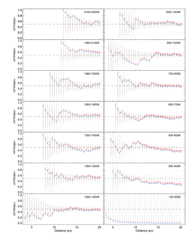
Figure 21: The average $V/V_{\rm max}$ value in 0.5-pc intervals for fourteen 150-K bins encompassing our 20-pc L, T, and Y dwarf census. Blue dots represent our empirical sample. Red labels mark the number of objects in the computation at each 0.5-pc interval. The black dashed line shows the $\langle{V}/{V_{max}}\rangle=0.5$ level indicating a complete sample. The grey error bars show the approximate 1$\sigma$ range around $\langle{V}/{V_{max}}\rangle$ = 0.5 that a complete sample of the size indicated by the red number would exhibit, given random statistics. The brown error bars, offset by +0.05 pc from the grey error bars for clarity, show the 1$\sigma$ variation around 0.5 obtained by 10,000 Monte Carlo simulations having the number of objects and completeness limit listed in Table 15.

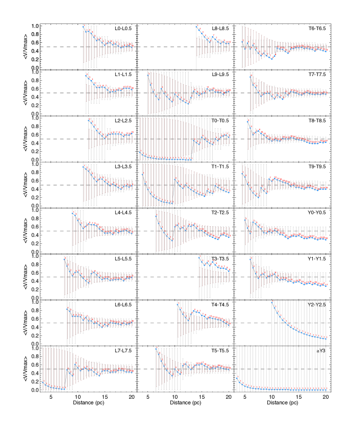
Figure 22: The average $V/V_{\rm max}$ value in 0.5-pc intervals for twenty-four integral spectral type bins encompassing our 20-pc L, T, and Y dwarf census. See the caption to Figure 21 for more details.

Using these methods, we find that our sample is likely complete to 20 pc for all bins between 600 and 2250K in $T_{\rm eff}$. For cooler bins the completeness limit drops to 15 pc for 450-600K and to 11 pc for 300-450K. (The coolest bin with data, 150-300K, has only one object in it, WISE 0855$-$0714, so the completeness cannot be computed.) We note, however, that the 300-450K bin is likely complete over only a fraction of its 150K interval because the coldest assigned $T_{\rm eff}$ for any object in this bin is 367K. We further note that two sources within the 525-object L, T, and Y dwarf 20-pc census – G 239-25B (1442+6603) and LSPM J1735+2634B – have assigned $T_{\rm eff}$ values (Table 11) that are hotter than the hottest temperature bin considered here. Finally, our measured space density in the 2100-2250K bin should be considered as a lower limit, too, because if we were to have included late-M dwarfs in our 20-pc census some fraction of them would have populated this bin. These results are shown in the first three columns of the upper portion of Table 15.

Bins of integral spectral subtype, which generally have poorer statistics can, by extension, be assumed complete out to 20 pc for types warmer than 600K, which is roughly late-T (Figure 20b). A close look at Figure 22 shows that the census appears to be complete for spectral types from L0 through T7.5. The completeness limit drops to $\sim$17 pc for types T8-T9.5 and to $\sim$13 pc for types Y0-Y1.5. Later types than this have only one representative per bin – WISE 1828+2650 at Y2 and WISE 0855$-$0714 at a type presumably later than that – so completeness limits cannot yet be determined. Results are shown in the first three columns of the lower portion of Table 15.

Table 15: Space Densities for Early-L through Early-Y Dwarfs

Teff or	Complete-	Raw	Adjusted	Corr.	Adopted
SpT	ness Limit	No. of	No. of	Factor	Space Density
Bin	(pc)	Objects	Objects		($\times$10-3 pc-3)
	$d_{max}$	$raw$	$adj$	$corr$	$dens$
(1)	(2)	(3)	(4)	(5)	(6)
2100-2250K	20.0	10	10.9$\pm$2.5	1.05	$>$0.31
1950-2100K	20.0	23	19.3$\pm$3.2	1.05	0.72$\pm$0.18
1800-1950K	20.0	16	21.2$\pm$3.6	1.05	0.50$\pm$0.17
1650-1800K	20.0	25	24.0$\pm$3.8	1.05	0.78$\pm$0.20
1500-1650K	20.0	26	24.7$\pm$3.9	1.05	0.81$\pm$0.20
1350-1500K	20.0	30	32.2$\pm$4.5	1.05	0.94$\pm$0.22
1200-1350K	20.0	60	50.9$\pm$5.2	1.09	1.95$\pm$0.30
1050-1200K	20.0	34	44.0$\pm$5.2	1.09	1.11$\pm$0.25
900-1050K	20.0	51	48.6$\pm$5.2	1.13	1.72$\pm$0.30
750-900K	20.0	59	58.4$\pm$5.8	1.13	1.99$\pm$0.32
600-750K	20.0	83	76.0$\pm$6.3	1.13	2.80$\pm$0.37
450-600K	15.0	53	44.9$\pm$4.9	1.13	4.24$\pm$0.70
300-450K	11.0	14	16.7$\pm$3.0	1.13	$>$2.84
150-300K	$\cdots$	1	$\cdots$	$\cdots$	$\cdots$
L0-L0.5	20.0	10	8.1$\pm$0.8	1.05	0.31$\pm$0.10
L1-L1.5	20.0	20	21.7$\pm$0.9	1.05	0.63$\pm$0.14
L2-L2.5	20.0	15	13.7$\pm$1.0	1.05	0.47$\pm$0.13
L3-L3.5	20.0	9	9.6$\pm$1.1	1.05	0.28$\pm$0.10
L4-L4.5	20.0	21	20.5$\pm$0.9	1.05	0.66$\pm$0.15
L5-L5.5	20.0	21	21.8$\pm$0.9	1.05	0.66$\pm$0.15
L6-L6.5	20.0	26	22.6$\pm$1.4	1.05	0.81$\pm$0.17
L7-L7.5	20.0	19	21.6$\pm$1.5	1.05	0.60$\pm$0.14
L8-L8.5	20.0	10	11.2$\pm$0.8	1.05	0.31$\pm$0.10
L9-L9.5	20.0	20	19.5$\pm$0.5	1.05	0.63$\pm$0.14
T0-T0.5	20.0	7	7.0$\pm$0.7	1.13	0.24$\pm$0.09
T1-T1.5	20.0	7	7.5$\pm$0.5	1.13	0.24$\pm$0.09
T2-T2.5	20.0	13	13.0$\pm$0.1	1.13	0.44$\pm$0.12
T3-T3.5	20.0	8	7.0$\pm$0.7	1.13	0.27$\pm$0.10
T4-T4.5	20.0	14	14.5$\pm$0.9	1.13	0.47$\pm$0.13
T5-T5.5	20.0	35	34.5$\pm$0.9	1.13	1.18$\pm$0.20
T6-T6.5	20.0	43	43.5$\pm$1.0	1.13	1.45$\pm$0.22
T7-T7.5	20.0	45	43.5$\pm$1.2	1.13	1.52$\pm$0.23
T8-T8.5	16.5	59	58.0$\pm$1.5	1.13	3.54$\pm$0.47
T9-T9.5	17.5	37	37.0$\pm$1.8	1.13	1.86$\pm$0.32
Y0-Y0.5	12.0	16	17.0$\pm$0.7	1.13	2.50$\pm$0.63
Y1-Y1.5	13.5	11	10.0$\pm$1.0	1.13	1.21$\pm$0.36
Y2-Y2.5	$\cdots$	1	$\cdots$	$\cdots$	$\cdots$
$\geq$Y3	$\cdots$	1	$\cdots$	$\cdots$	$\cdots$

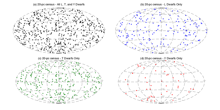
Figure 23: Plots of the 20-pc L, T, and Y dwarf sample in equatorial coordinates. The four panels display the sample in its entirety (black), only the L dwarfs (blue), only the T dwarfs (green), and only the Y dwarfs (red).

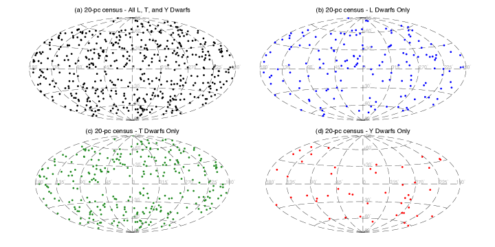
Figure 24: Plots of the 20-pc L, T, and Y dwarf sample in Galactic coordinates. See the caption to Figure 23 for more details.

The bins in our $T_{\rm eff}$ and spectral type histograms are fixed, but our confidence in placing an object in a particular bin is directly related to the uncertainties in these quantities. For example, some of our objects have errors on $T_{\rm eff}$ that are comparable to our 150K bin size, and the errors on some of our spectral types are also comparable to the integral spectral type bin size used. The lack of precision in these values is our biggest uncertainty in fixing the space densities in each bin. To address what the size of this uncertainty should be, we have run 10,000 Monte Carlo simulations for both the $T_{\rm eff}$ and spectral type distributions. For $T_{\rm eff}$ we have taken the error bars listed in Table 11, which were taken either from literature values (see Table 14) or assigned via the root-mean-square scatter from whichever relation in Table 13 was used for the $T_{\rm eff}$ estimate. For spectral type, we have assigned the standard 0.5-subclass uncertainty to all types except those with uncertainties already specified explicitly or for those with brackets or colons, for which we have assigned 1.0-subclass uncertainties. For each simulation, we take the $T_{\rm eff}$ or spectral type uncertainty, and multiply it by a random value generated from a normal distribution having a mean of 0 and a standard deviation of 1. We add this uncertainty onto the measured value, and then rebin. We then compute the means and standard deviations across all 10,000 simulations and report these in column 4 of Table 15.

These simulations have a drawback, however, because the $T_{\rm eff}$ bins at either end of our 150-2250K range are incomplete. Firstly, the 1950-2100K bin will contain objects that scatter into the 2100-2250K bin, but this loss in the cooler bin will not be mitigated by a concomitant gain from the warmer bin because the object count in that latter bin is incomplete. Secondly, over the 300-750K range, we encounter differing completeness limits in distance across the three bins that span this range as well as having an incompleteness in temperature in the 300-450K bin. For example, objects that scatter from the 600-750K bin into the 450-600K bin will be lost if they have a distance larger than the completeness limit of that colder bin. Objects scattering in the other direction will not be similarly lost. The same is true of objects scattering between the 450-600K bin and the 300-450K bin. Given these biases, we adopt a methodology whereby we use the raw number counts in each bin to set the space density, but we use the uncertainties from the simulations to set a conservative limit on their 1$\sigma$ errors.

Although most of our bins pass the $\langle{V}/{V_{max}}\rangle$ completeness test to 20 pc, this does not address whether there are inhomogeneities in the all-sky distribution. Kirkpatrick et al. (2019) found an inhomogeneity in the T and Y dwarf counts toward the Galactic Plane, in which source confusion limits our ability to select objects in the faintest, coldest bins. We re-investigate this here. Plots of our all-sky distributions broken down by broad spectral class are shown in Figures 23 and 24. The plot of T dwarfs appears to show a thinner area of coverage around and just south of the Galactic Plane in Figure 24c.

We address this further by dividing objects in our 20-pc census into two sectors, one for the objects having an absolute Galactic latitude ($|glat|$) $<14{\fdg}48$ (the "Plane" sector) and the second for objects having $|glat|\geq 14{\fdg}48$. This cut on $glat$ was selected so that the first sector covers one quarter of the sky and the second covers the other three quarters. For each temperature and spectral type bin, we can therefore determine if the numbers in the Plane sector, when tripled, appear to be significantly lower than those found in the second sector. Using the complete samples as defined in Table 15, we find 27 Y0-Y1.5 dwarfs. Of these, 23 lie outside of the Plane sector, meaning that we would expect $23/3\approx 8$ similar objects to lie in the Plane sector itself. However, only 4 are found there, for a shortfall of 4, or 15% of the total sample. Using the same methodology and combining spectral bins to increase the statistical significance of each binned population, we find shortfalls of 13% for T8-T9.5 (96 objects total), 10% for T6-T7.5 (88 objects total), 14% for T4-T5.5 (49 objects total), 12% for T0-T3.5 (35 objects total), 5% for L6-L9.5 (75 objects total), and 5% for L0-L5.5 (96 objects total). We thus apply an adjustment factor of 1.05 across the L dwarf densities and 1.13 across the T and Y dwarf densities. We apply these same factors to the $T_{\rm eff}$-based densities, and use an average adjustment factor of 1.09 to the 1050-1350K bins that cross the L/T transition. These factors are listed in the fourth column of Table 15. To compute the space densities, we used the formulae given in the footnotes of Table 15. These final values are given in column 6 and are represented graphically in Figure 25.

We can compare these results to other recent determinations in the literature. At early-L types, Bardalez Gagliuffi et al. (2019) find space densities of [0.75$\pm$0.13, 1.02$\pm$0.16, 0.78$\pm$0.14, 0.58$\pm$0.12, 0.88$\pm$0.15, 1.44$\pm$0.19] ${\times}10^{-3}{\rm pc}^{-3}$ per integral spectral type bins of [L0-L0.5, L1,L1.5, L2-L2.5, L3-L3.5, L4-L4.5, L5-L5.5]. Our space density determinations across each of these bins differ by an average of 2.1$\sigma$, and the Bardalez Gagliuffi et al. (2019) results are consistently a factor of $\sim$1.9 higher. However, Bardalez Gagliuffi (priv. comm.) find that their published densities included a pessimistic set of assumptions in their completeness calculation. Our Table 15 values compare favorably to the $T_{\rm eff}$-binned values of Kirkpatrick et al. (2019), the biggest deviations being a 1.2$\sigma$ variation (difference factor of 0.84 between Kirkpatrick et al. 2019 and this paper) in the 750-900K bin and a 1.4$\sigma$ variation in the opposite direction (difference factor of 1.27) in the adjacent 600-750K bin.

Figure 25: Our measured space densities from Table 15. (Top) Space densities as a function of effective temperature. (Bottom) Space densities as a function of near-infrared spectral type.

9 Determining the Mass Function

In Kirkpatrick et al. (2019) we developed a formalism for translating various forms of the mass function into the observational domain, since mass is not an observable quantity for most objects within the 20-pc census. There are several steps in doing this, which we summarize below.

First, we considered a variety of functional forms of the mass function that have been proposed in the literature. These include power laws ($dN/dM\propto M^{-\alpha}$) with $\alpha$ values ranging from $-$1.0 to 1.5, the log-normal distribution ($dN/dM\propto e^{-(ln(M)-\mu)^{2}/2\sigma^{2}}$) with values of the mean ($\mu$) and standard deviation ($\sigma$) taken from Chabrier (2001), Chabrier (2003a), and Chabrier (2003b), and a bi-partite power law favored by Kroupa et al. (2013). These forms determine the distribution of masses produced.

Second, a stellar birthrate that has remained constant in time over the past 10 Gyr was assumed. Burgasser (2004) found that the stellar luminosity function for T dwarfs is largely invariant to the birthrate assumed, although the L dwarf regime can still bear an imprint from recent events if star formation is more episodic. Allen et al. (2005) explored this further and found that changes in the luminosity function produced by the underlying mass function were much larger than those produced by variations in the birthrate.

Third, because most of the objects in our simulations are brown dwarfs, the observable quantity we use for the empirical determinations ($T_{\rm eff}$) changes with time as the brown dwarf ages and cools. Hence, we tie each simulated object to an evolutionary path applicable to its mass, so that we can determine its current $T_{\rm eff}$. Two sets of evolutionary models were employed for this, resulting in two different sets of simulated $T_{\rm eff}$ distributions. The first were the solar-metallicity COND models from Baraffe et al. (2003) that, because they neglect dust opacity, are most applicable to mid-M dwarfs and mid- to late-T dwarfs believed to be free of photospheric clouds. These model grids are sampled at five different ages (0.1, 0.5, 1, 5, and 10 Gyr) and sample the temperature range $125K\lesssim T_{\rm eff}\lesssim 2800K$, which corresponds to masses around $0.01M_{\odot}<M<0.10M_{\odot}$. The second set of models were the hybrid suite of solar-metallicity models from Saumon & Marley (2008) that assume cloud-free atmospheres only in the late-M and late-T zones but account for cloud growth and subsequent clearing in and around the transition from L dwarfs to T dwarfs. The evolutionary model grids are sampled at twenty-six different ages in the 3 Myr $<$ age $<$ 10 Gyr range and cover the range $300K\lesssim T_{\rm eff}\lesssim 2400K$, which corresponds to the mass range $0.002M_{\odot}<M<0.085M_{\odot}$.

Fourth, we used the inverse transform sampling method to turn the various forms of the mass function into space densities binned in $T_{\rm eff}$. The process is as follows. Each normalized mass function can be used as a probability density function, which gives the likelihood of drawing at random an object of a certain mass from within that distribution. In a practical sense, this random drawing is done by integrating under the probability density function to produce a cumulative distribution function, reversing the dependent and independent variables, and re-solving for the dependent variable, thus creating the inverse cumulative distribution function which then provides a mapping from the a random seed to an actual mass. The seed is produced via a random sampling of a uniform distribution over the range zero to one.

Fifth, we performed the simulations by creating $3{\times}10^{6}$ random seeds, each of which was assigned an age according to its order of selection. These ages were distributed uniformly over the subset of 0-10 Gyr interval over which each evolutionary model is valid. The seed was then passed through the inverse cumulative distribution function to assign its mass, then the assigned age and mass were passed through the evolutionary models to get the current $T_{\rm eff}$. Because the evolutionary models are sampled only on a sparse grid, bilinear interpolation between neighboring points was used to assign the temperature.

Finally, simulations were produced for each of the twelve assumed functional forms of the mass function, each of which was run through the two different evolutionary model grids. Furthermore, each simulation was run with three different values of a cutoff mass (10$M_{Jup}$, 5$M_{Jup}$, or 1$M_{Jup}$,), which is the lowest mass product that can be created. This resulted in a grid of seventy-two simulated $T_{\rm eff}$ distributions.

9.1 Mass Function Fits

Here, we have compared our measured space densities to these seventy-two simulations. To determine the simulation that fits best, we have used the IDL routine mpfit (Markwardt 2009) to perform a weighted least-squares fit between the data and the simulations, where the only adjustable parameter is the scaling between the arbitrary number counts in the models and our measured space densities. For the calculation, we use only the eleven values in the upper portion of Table 15 that cover the range 450-2100K, as the other values are lower limits only. The best fit to each model produces a reduced $\chi^{2}$ value.

Figure 26 shows the fits for which this value is minimized. These best fits are identical to the best fits found by Kirkpatrick et al. (2019), and involved the single power law and log-normal forms. For each evolutionary model, the power law form is slightly favored over the log-normal based on the best-fit $\chi^{2}$ minimization values. In contrast to the results of Kirkpatrick et al. (2019), we now find that the evolutionary code of Saumon & Marley (2008) is highly favored over that of Baraffe et al. (2003), and the reason for this is the inclusion in this paper of space density measurements over the cloudy-to-clear transition that the Saumon & Marley (2008) models were designed to address. Specifically, the space density spike in the 1200-1350K bin of Figure 26 is well produced by simulations incorporating the Saumon & Marley (2008) models, and this bin is the one covering spectral types from $\sim$L8 to $\sim$T3 (the yellow zone in Figure 20b) over which cloud building and subsequent break-up have been hypothesized. These models not only predict the position of the spike but also correctly predict its magnitude. Furthermore, they also predict the magnitude of the drop-off and recovery at cooler types once clouds have cleared and cooling once again proceeds as normal.

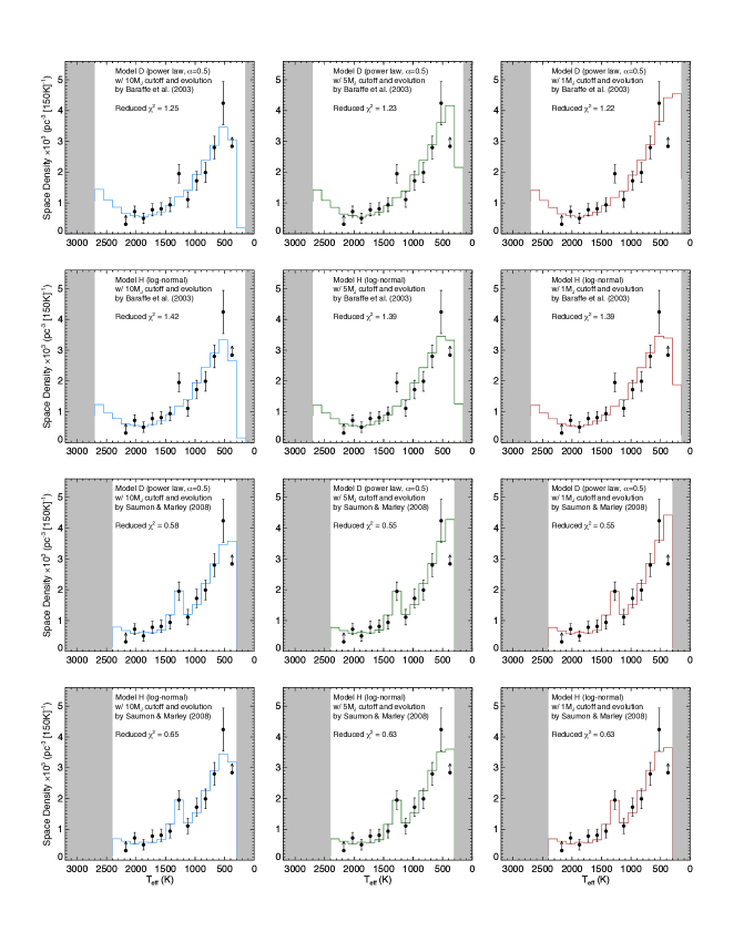
Figure 26: The best fits between the simulations and our measured space densities. Of the simulations that use the evolutionary tracks of Baraffe et al. (2003), the two with the smallest reduced $\chi^{2}$ values are shown in the top two rows. Of the simulations that use the evolutionary tracks of Saumon & Marley (2008), the two that provide the best fits are show in the two bottom rows. "Model D" refers to the power law with $\alpha=0.5$, and "Model H" refers to the single-object log-normal form of Chabrier (2001). See Kirkpatrick et al. (2019) for additional information on these simulations. Each row shows the same model with a different low-mass cutoff: 10$M_{Jup}$ (blue) in the left panel, 5$M_{Jup}$ (dark green) in the middle panel, and 1$M_{Jup}$ (red) in the right panel. Our measured space densities and their uncertainties are shown in black. Grey zones denote areas not covered by the simulations.

The best fits across the coarse grid of 72 models are those with the single power law of $\alpha=0.5$. Figure 27 illustrates a few supplemental simulations to show that the minimum $\chi^{2}$ value across a finer grid of models is actually reached at $\alpha=0.6$, which was the same conclusion found by Kirkpatrick et al. (2019). There is however, no significant difference between the $\chi^{2}$ values of the $\alpha=0.5$, 0.6, and 0.7 models. Obtaining a more accurate space density in the 450-600K bin is critical to pinning down the true value of $\alpha$.

As a closer look at Figure 27 reveals, the preferred value of $\alpha$ rests largely with the steepness of the curve over the 1200-450K region, and most of the power falls in that region’s final bin (450-600K), for which the space density is the highest. If we use the densities implied by our temperature randomizations (column 4 of Table 15), we find a best fit of $\alpha=0.4$, although, as discussed earlier, the density for that bin is likely biased low. This leads us to conclude that our measurements of the space density support a value of $\alpha=0.6{\pm}0.1$.

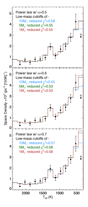
Figure 27: Fits of power laws with $\alpha=0.5$ (top panel), $\alpha=0.6$ (middle panel), and $\alpha=0.7$ (bottom panel) to our observational data (black points). These predicted $T_{\rm eff}$ distributions have been passed through the evolutionary models of Saumon & Marley (2008). Each panel shows simulations for three low-mass cutoffs: 10 $M_{Jup}$ (blue), 5 $M_{Jup}$ (green), and 1 $M_{Jup}$ (red). The minimum reduced $\chi^{2}$ values are found for the $\alpha=0.6$ model.

9.2 The Low-mass Cutoff

Whereas the 450-600K bin is critical in determining the value of the power law’s exponent, the next cooler bins are critical in determining the cutoff mass. The best fits to our observed space densities currently do not have a strong dependence on the low-mass cutoff. As the plots in Figure 27 show, this is because the lower limit to the density in the 300-450K bin is consistent with all three values of the cutoff mass (10, 5, and 1 $M_{Jup}$ ). An increase of just 40% in the value of this lower limit would enable us to confidently claim a cutoff mass below 10$M_{Jup}$. (In Kirkpatrick et al. 2019 we had claimed to push the cutoff mass below 5$M_{Jup}$, but this was based on a number of objects in the 300-450K bin that was half as large as the sample we are now using.) This bin is comprised mostly of Y0.5 to Y2 dwarfs (Figure 20b), which are challenging objects to uncover given their faint absolute magnitudes ($M_{J}\approx M_{H}>23$ mag, $M_{W2}=M_{\rm ch2}>15$ mag; Figure 14).

Even more critical to defining the low-mass cutoff is the next cooler bin, 150-300K, which presently has only one known object in it, WISE 0855$-$0714. Finding more representative objects in this bin would even more readily determine the cutoff mass, as the top row of Figure 26 shows. For the $\alpha=0.5$ model, the space density values in this bin vary wildly – from ${\sim}0.2{\times}10^{-3}{\rm pc}^{-3}$ for a 10$M_{Jup}$ cutoff, to ${\sim}2.2{\times}10^{-3}{\rm pc}^{-3}$ for a 5$M_{Jup}$ cutoff, to ${\sim}4.5{\times}10^{-3}{\rm pc}^{-3}$ for a 1$M_{Jup}$ cutoff. Finding objects in this bin is an even more challenging proposition, as WISE 0855$-$0714 itself has absolute magnitudes of $M_{J}\approx 28$ mag, $M_{H}\approx 27$ mag, and $M_{W2}=M_{\rm ch2}\approx 17$ mag.

Nonetheless, we can use objects of known mass within the 20-pc census to help further refine the cutoff value. Most notably, a number of census members are known to belong to young moving groups and associations (section 7.1), and these objects will have hotter temperatures and earlier spectral types than older counterparts in the field of the same mass. Hence, finding an object of exceedingly low mass is a far less daunting challenge if is it younger and brighter. Young members of the 20-pc census are listed along with their assigned $T_{\rm eff}$ values and published masses in Table 16.

Before exploring these masses, though, we note that such determinations are direct comparisons to evolutionary models and thus fail to provide an independent check of the theory. Are the masses coming from the evolutionary models trustworthy? To answer this, we have also listed in Table 16 those multiple systems within the 20-pc census whose masses have been measured dynamically. These objects are identified with their corresponding $T_{\rm eff}$ bin and indicated in Figure 28. This figure shows, for both the Saumon & Marley (2008) and Baraffe et al. (2003) evolutionary tracks, the expected mass distributions from our simulations for each of our 150K bins. The simulations show a tight distribution of masses for the hotter bins, but the range of masses quickly expands for the colder bins. In the Saumon & Marley (2008) models, a wide range of masses is expected to inhabit each of the temperature bins from 750K to 1500K. At colder temperatures, though, the mass range reduces dramatically, with the 300-450K bin containing only objects with masses below $\sim 30M_{Jup}$. (Using the Baraffe et al. 2003 models, which explore even colder temperatures, we find that the mass range shrinks to $<15M_{Jup}$ for the 150-300K bin.)

For the warm bins with the narrowest mass distributions (2100-2250K and 1950-2100K), the two objects in Table 16 with dynamical measures have masses in accordance with the model predictions. Good agreement is seen at cooler bins as well. The only objects with measures that may be discrepant with expectations are the four objects in the 1650-1950K range (Gl 584B and C, DENIS 2252+1730A, 2MASS 0700+3157A) in panel (a), the highest mass object in the 1200-1350K bin (Gl 845B) along with the two objects in the 900-1050K bin (Gl 229B and Gl 845C) of both panels, and the three lowest mass objects (SDSS 0423$-$0414B and WISE 1049$-$5319AB) in the 1200-1350K bin of panel (b). These latter three objects can be explained as the inability of the older Baraffe et al. (2003) models to account for clouds in this range, since these objects do not appear unusual when compared to the expectations from Saumon & Marley (2008).

Figure 28: Simulated mass distributions for each of the 150K $T_{\rm eff}$ bins. (a) The single power law of $\alpha=0.5$ coupled with the Saumon & Marley (2008) evolutionary tracks. (b) The same, but coupled with the Baraffe et al. (2003) evolutionary tracks. Because the Saumon & Marley (2008) models do not extend below 300K, the bin at lower right in panel (a) is empty. For ease of comparison, the same $x$ and $y$ scaling is used for all subpanels. Objects from Table 16 that have dynamically measured masses (filled black stars) are plotted in their $T_{\rm eff}$ bins at the $x$ location corresponding to their mass; their $y$ positions are arbitrary.

The other objects deserve closer scrutiny:

• Gl 564BC: This pair has masses lower than 85% of objects in the 1650-1800K bin. Objects of this mass, according to our simulations, would have a relatively young age of $\sim$580$\pm$67 Myr. Potter, et al. (2002) note that the primary in this system, the G2 dwarf Gl 564A, is chromospherically active, a fast rotator, and an object of high lithium abundance, which places its age at $<$800 Myr. After a more careful analysis, Dupuy et al. (2009) adopt an age for the primary of $790^{+220}_{-150}$ Myr, which accords with the young age expected by our simulations.

• DENIS 2252$-$1730A: The is the third other object in the 1650-1800K bin. It has a dynamical mass intermediate between Gl 564B and Gl 564C and would thus be expected from our simulations to have a similarly young age. However, there does not appear to be independent verification of a young age in the literature, such as a measurement of lithium absorption in the A component (Dupuy, & Liu 2017).

• 2MASS 0700+3157A: This object falls in the 1800-1950K bin. Our simulations find that it has a mass lower than 85% of objects in its temperature bin, implying another relatively young age of 755$\pm$101 Myr. There is no independent assessment of age for this object, although Dupuy, & Liu (2017) also note the model-implied young age for the primary. As stated in that work, Thorstensen & Kirkpatrick (2003) report no lithium in the joint spectrum of the AB pair, which would likely mean only that the age is $>$200 Myr.

• Gl 845BC: The masses of both components are surprisingly high for their respective temperature bins. In our simulations that use the Saumon & Marley (2008) evolutionary models, we find $\sim$250,000 objects in our 3-million-object simulation that fall in the 1200-1350K bin inhabited by Gl 845B but none of these simulated objects has a mass as high as Gl 845B. Likewise, of our $\sim$190,000 simulated objects in the 900-1050K bin, none has a mass as high as Gl 845C. This system is not believed to be exceptionally old, either (see Dieterich et al. 2018), which might partly explain the ultra-high masses. Switching to the Baraffe et al. (2003) evolutionary code instead gives a similar result. The published mass measurements for this system are completely at odds with theoretical expectations.

• Gl 229B: This object has an ultra-high mass for its effective temperature. Its measured mass is almost identical to that of Gl 845C, so the arguments for Gl 845C above also apply to Gl 229B. Brandt et al. (2020) note that an exceptionally old age for the Gl 229 system is disfavored, making Gl 229B another T dwarf whose mass measurement is at odds with expectations.

In summary, then, the masses expected from our simulations are consistent with the measured dynamical masses in Table 16 for most objects for which direct comparisons can be done. The exceptions are Gl 229B and Gl 845BC, which remain puzzles.

The consistency between most of the measurements and the expected values at higher masses gives us a cautious confidence – but not independent confirmation – in trusting model-implied values at lower masses. Of the 20-pc moving group members listed in Table 16, the ones of lowest mass are between 10 to 12 $M_{Jup}$. So, within the 20-pc census, we are not able to push the cutoff mass below 10 $M_{Jup}$ through either a critical analysis of the entire L, T, and Y sample or through an analysis of the subset with moving group membership. Despite this limitation, we can look at the young moving group members in a larger sample volume, which strongly hint at a low-mass cutoff substantially below 10 $M_{Jup}$. As discussed in section 7.1, PSO J318.5338$-$22.8603, 2MASSW J1207334$-$393254b, and 2MASS J11193254$-$1137466AB are believed to have masses in the 4-7 $M_{Jup}$ range, and other objects identified in Table 12 could possibly lower the limit within the 20-pc census itself.

Table 16: Masses for L, T, and Y Members of the 20-pc Census

Object	Sp.	Teff	Mass	Method	Mass
	Type	(K)	(MJup)		Ref.
(1)	(2)	(3)	(4)	(5)	(6)
2MASS 0045+1634	L2$\gamma$	2059$\pm$45	$24.98{\pm}4.62$	MovGp	F
WISE 0047+6803	L6-8$\gamma$	1230$\pm$27	$11.84{\pm}2.63$	MovGp	F
SIMP 0136+0933	T2	1051$\pm$198	$12.7{\pm}1.0$	MovGp	G
2MASS 0355+1133	L3-6$\gamma$	1478$\pm$58	$21.62{\pm}6.14$	MovGp	F
SDSS 0423-0414A	L6.5:	1465$\pm$134	$51.6^{+1.5}_{-2.5}$	dynam	D
SDSS 0423-0414B	T2	1218$\pm$79	$31.8^{+1.5}_{-1.6}$	dynam	D
AB Dor Cb(0528-6526)	$\cdots$	$\cdots$	$14{\pm}1$	MovGp	C
Gl 229B(0610-2152)	T7 pec	927$\pm$77	$70{\pm}5$	dynam	A
2MASS 0700+3157A	L3:	1838$\pm$134	$68.0{\pm}1.6$	dynam	D
2MASS 0700+3157B[C]	L6.5:	1465$\pm$134	$73.3^{+2.9}_{-3.0}$	dynam	D
WISE 0720-0846B	[T5.5]	1183$\pm$88	$66{\pm}4$	dynam	T
2MASS 0746+2000A	L0	2237$\pm$134	$82.4^{+1.4}_{-1.5}$	dynam	D
2MASS 0746+2000B	L1.5	2029$\pm$134	$78.4{\pm}1.4$	dynam	D
WISE 1049-5319A	L7.5	1334$\pm$58	$34.2^{+1.3}_{-1.1}$	dynam	V
WISE 1049-5319B	T0.5:	1261$\pm$55	$27.9^{+1.1}_{-1.0}$	dynam	V
SDSS 1110+0116	T5.5	926$\pm$18	10-12	MovGp	I
LHS 2397aB(1121-1313)	[L7.5]	1282$\pm$88	$66{\pm}4$	dynam	D
2MASS 1324+6358	T2: pec	1051$\pm$197	11-12	MovGp	H
DENIS 1425-3650	L4$\gamma$	1535$\pm$53	$22.52{\pm}6.07$	MovGp	F
Gl 564B(1450+2354)	L4	1722$\pm$134	$59.8^{+2.0}_{-2.1}$	dynam	D
Gl 564C(1450+2354)	L4	1722$\pm$134	$55.6^{+2.0}_{-1.9}$	dynam	D
2MASS 1534-2952A	T4.5	1172$\pm$79	$51{\pm}5$	dynam	D
2MASS 1534-2952B	T5	1125$\pm$79	$48{\pm}5$	dynam	D
LSPM 1735+2634B	L0:	2274$\pm$88	$87{\pm}3$	dynam	D
Gl 758B (1923+3313)	T7:	581$\pm$88	$37.9^{+1.4}_{-1.5}$	dynam	B
Gl 779B (2004+1704)	L4.5$\pm$1.5	1533$\pm$88	$72.7{\pm}0.8$	dynam	B
Gl 802B (2043+5520)	[L5-L7]	1483$\pm$88	$66{\pm}5$	dynam	M
Gl 845B (2204-5646)	T1	1236$\pm$79	$75.0{\pm}0.8$	dynam	S
Gl 845C (2204-5646)	T6	965$\pm$79	$70.1{\pm}0.7$	dynam	S
2MASS 2244+2043	L6-8$\gamma$	1184$\pm$10	$10.46{\pm}1.49$	MovGp	F
DENIS 2252-1730A	[L4:]	1722$\pm$134	$59{\pm}5$	dynam	D
DENIS 2252-1730B	[T3.5]	1190$\pm$79	$41{\pm}4$	dynam	D

Note. — Legend for method: MovGp = mass comes from evolutionary models combined with the known age of the moving group or young association with which this object is a member; dynam = mass is measured dynamically.

Note. — Reference code for mass determination: A = Brandt et al. 2020, B = Brandt et al. 2019, C = Climent et al. 2019, D = Dupuy, & Liu 2017, F = Faherty et al. 2016, G = Gagné et al. 2017, H = Gagné et al. 2018, I = Gagné et al. 2015, M = Ireland et al. 2008, S = Dieterich et al. 2018, T = Dupuy et al. 2019, V = Garcia et al. 2017.

9.3 The Age Distribution

We can also compare the expected age distributions with our limited knowledge of the ages for objects in the census. Figure 29 shows plots analogous to the mass distributions shown in Figure 28. For the Saumon & Marley (2008) evolutionary tracks in the 900-2250K regime, the age distributions cover the entire range of 0-10 Gyr ages but with a skew toward young ages. The age distribution then flattens across the 600-900K range, although the youngest ages ($<$0.5 Gyr) start to disappear. A skew toward old ages appears below 600K, with the skew becoming more severe with higher cutoff mass. The Baraffe et al. (2003) evolutionary tracks show that this skew toward old ages is exacerbated in the coldest bin (150-300K). Here, a 10 $M_{Jup}$ cutoff mass would imply no objects with ages $<$7 Gyr, whereas a 1 $M_{Jup}$ cutoff would give a much more uniform age distribution, albeit with few objects having ages below 1 Gyr.

Figure 29: Simulated age distributions for each of the 150K $T_{\rm eff}$ bins. (a) The single power law of $\alpha=0.5$ coupled with the Saumon & Marley (2008) evolutionary tracks. (b) The same, but coupled with the Baraffe et al. (2003) evolutionary tracks. Because the Saumon & Marley (2008) models do not extend below 300K, the bin at lower right in panel (a) is empty. For ease of comparison, the same $x$ and $y$ scaling is used for all subpanels. The colored triangles along the bottom edge of each subpanel show the median age for cutoff masses of 10$M_{Jup}$ (blue), 5$M_{Jup}$ (green), and 1$M_{Jup}$ (red); these triangles overlap in all but the coldest bins.

Most of the objects in the 20-pc L, T, and Y dwarf census lack age information, but we can examine this using tangential velocities as proxies of dynamical heating. Figure 30 shows the census’ total proper motion and tangential velocity distributions. A total of 2% of the objects – nine in total – have $v_{tan}>100$ km s^-1. These objects are 2MASS 0251$-$0352 (112 km s^-1), 2MASS 0645-6646 (139 km s^-1), WISE 0833+0052 (106 km s^-1), 2MASS 1126$-$5003 (127 km s^-1), 2MASS 1231+0847 (106 km s^-1), DENIS 1253$-$5709 (128 km s^-1), 2MASS 1721+3344 (151 km s^-1), WISE 2005+5424 (129 km s^-1), and Gl 802B (154 km s^-1). Three of these are subdwarfs discussed in section 7.2, one is a possible subdwarf discussed in section 7.6, two are blue/peculiar L dwarfs, and one is a companion to a mid-M binary believed to be $\sim$10 Gyr old (Ireland et al. 2008).

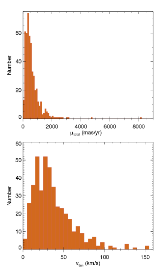
Figure 30: Histograms of the total proper motion and $v_{tan}$ for the L, T, and Y dwarfs in the 20-pc census. In the upper diagram, the total motion is shown for all systems in the census. In the lower diagram, the tangential velocity is shown only for those systems having parallax measures with uncertainties below 12.5%. The median $v_{tan}$ value for objects in the lower panel is 30.8 km s^-1.

For the entire 20-pc census, we can check whether the expected inflation of the velocities at older ages is seen in our empirical data. To accomplish this, we compare the median ages expected from our simulations to the median $v_{tan}$ values from our actual measurements. In Figure 29 we illustrate the median age at each 150K bin for our $\alpha=0.5$ power law simulation. We also plot the measured tangential velocity against effective temperature in Figure 31, along with the median tangential velocity value in each of the 150K bins. In Figure 29, we see that the median age shifts to younger values from 2250K down to 1500K and reaches a minimum in the 1350-1500K bin before reversing course and trending to increasingly older values for increasingly cooler bins. Our measured $v_{tan}$ values in Figure 31 show only a little variation across the 500-2250K regime but increase substantially in the 300-450K bin.

Although the agreement is qualitatively the same – in the sense that the colder, older objects have higher velocities indicative of dynamical heating – the coldest portion of our sample may be biased toward higher velocities anyway. Objects in the coldest bins are Y dwarfs that are uncovered almost exclusively with WISE data and should have very red colors of W1$-$W2 $>$ 4 mag. However, given their intrinsic faintness, they are usually not detected at W1, leading to W1$-$W2 color limits only. As the W2 mags themselves grow fainter, this color limit becomes less useful, and thus a detection of proper motion is the best way to discern W2-only Y dwarfs from background chaff. This reliance on a proper motion signature – which at faint magnitudes is itself only reliable if the motion is large – leads to a kinematic bias. Thus, the larger median velocity in the 300-450K bin may be a consequence of relying more heavily on motion as a selection criterion.

9.4 Where are the WISE 0855$-$0714 Analogs?

In the next fainter bin, 150-300K, WISE 0855$-$0714 is the only object recognized despite concentrated efforts to find other examples by both the Backyard Worlds and CatWISE teams. (With additional follow-up, WISE 0830+2837 from Bardalez Gagliuffi et al. 2020 may prove to be the second known member of this $T_{\rm eff}$ bin.) As Figure 29b demonstrates, objects in this bin should be heavily skewed old unless the low-mass cutoff is substantially less than 1$M_{Jup}$. Such a heavy skew to old ages also implies that such objects will be on average more metal poor than the Sun.

It is possible that analogs to WISE 0855$-$0714 have already been cataloged in the thousands of faint motion candidates already identified by the Backyard Worlds and CatWISE teams but remain unrecognized? After all, many of the objects have W1$-$W2 color limits only and were never imaged by Spitzer to provide more diagnostic ch1$-$ch2 colors. The answer is almost certainly "no," for the following reason. One of the criteria used to prioritize follow-up observations is the reduced proper motion, $H_{W2}=W2+5\log{\mu_{tot}}+5$, which is a crude measure of the object’s intrinsic faintness based on its apparent magnitude and the size of its transverse motion. If any of the motion candidates lacking solid color had distinguished themselves with an exceptionally faint $H_{W2}$ value – WISE 0855$-$0714 has $H_{W2}=23.4$ mag (Figure 1 of Bardalez Gagliuffi et al. 2020) – it would certainly have been noticed. WISE 0830+2837 from Bardalez Gagliuffi et al. (2020), with $H_{W2}=22.6$ mag, is the nearest contender now known.

Four possible scenarios to explain our lack of success in finding additional objects in the 150-300K bin are (1) they are exceedingly rare, (2) their intrinsic faintness places them too close to the W2 detection limit of WISE for motion searches to identify them confidently, (3) their motions are so high that coadds cannot be used to push the WISE detection limits deeper, and (4) their colors and magnitudes differ significantly from expectations. We discuss each of these scenarios below:

(1) The coldest objects are rare: Our result that the mass function is best fit with a power law of $\alpha=0.6$ and that the cutoff mass is likely at or below 5$M_{Jup}$ would imply a distribution of objects in the 150-300K bin like that shown in the green curve in the lower right panel of Figure 29b. This implies a space density of at least $2{\times}10^{-3}pc^{-3}$, which makes objects in this bin as common as T6 or T7 dwarfs. It is thus hard to reconcile these results with the hypothesis that such cold objects are extremely rare. Furthermore, it would be an unbelievable stroke of luck that our Sun falls a mere 2.3 pc from such an extremely rare, cold object, as it does with WISE 0855$-$0714. So we reject rarity as a possible cause.

(2) WISE is too shallow: History has shown us that all-sky surveys can lead to curious results when researchers push those surveys near their limits. The bottom of the main sequence in the 1980s appeared to fall at late-M (Probst & Liebert 1983; Reid 1987) based on the dominant discovery engine of its time, the Palomar Observatory Sky Survey (Minkowski & Abell 1963; Reid et al. 1991). We now know, of course, that the reason for this is the low space density of early-L dwarfs (see Figure 27) and the fact that the POSS-I and POSS-II $B$ and $R$ plates failed to survey enough volume to detect all but the nearest L dwarf examples. The L/T pair WISE 1049$-$5319 is present on the southern UK Schmidt photographic plates but was not selected as a motion source (Luhman 2013); we find that Willem Luyten, despite having cataloged over 58,000 proper motion stars using photographic data (Luyten 1979), failed to catalog any of the 20-pc L dwarfs in Table 11. In the case of WISE, Wright et al. (2014) have used the relatively bright W2 magnitude of WISE 0855$-$0714 (W2 = 13.82 mag), its distance (2.3 pc), and the fact that it lies $\sim$2 magnitudes above the limit of the AllWISE Catalog to argue that there should be another 4 to 35 similar objects already detected in AllWISE itself. The CatWISE and CatWISE2020 Catalogs (see below) have increased the sensitivity to lower motions at fainter magnitudes, thus making the identification of these detected objects even easier. Hence, it is unlikely that the survey that found WISE 0855$-$0714 is too shallow to find other analogs.

(3) High motions confound deeper searches: The data sets using the longest time baseline of WISE data are CatWISE Preliminary (Eisenhardt et al. 2020) and CatWISE2020 (Marocco et al. 2020b). Most points on the celestial sphere are visited by WISE during a several-day window every six months. Both the CatWISE Preliminary and CatWISE2020 processing leveraged these repeats to measure proper motions of all sources. Full-depth coadditions, which took all of the available data to create a single, deep image, were used for source detection. Those source detections were then characterized through the stack of epochal coadds (from each six-month window) to measure photometry and astrometry for each source. Sources with significant proper motions could then be selected from the resulting source tables. Sources that fail to move a significant portion of a full-depth coadd’s W2 FWHM (${\sim}6\arcsec$; Meisner et al. 2019) benefit from the coaddition, as their S/N increases by roughly the square root of the number of epochs. However, sources with higher motions do not see this benefit; a very high motion source will appear as a tracklet of separate sources in the full-depth coadd, and each separate apparition contains the background noise component from all epochs but the source signal from only one. Therefore, faint, high-motion sources can be lost in this process. If many of the coldest brown dwarfs are older kinematically, as Figure 29a and b suggest, their concomitant high proper motions may quash their identification by the CatWISE pipeline.

(4) Cold objects have unexpected colors or magnitudes: The analysis from Wright et al. (2014) inherently assumed that WISE 0855$-$0714 is a representative member of the Y dwarfs populating the 150-300K bin. What if WISE 0855$-$0714 is atypical? It has $v_{tan}=88.0$ km s^-1, which, although in the highest 4% of all $v_{tan}$ values in Figure 31, is not exceptional. If the majority of objects in the 150-300K bin are much older and have higher kinematics, then their high motions may suggest that point (3) above is a contributing cause. In addition, however, their older ages would also suggest a somewhat lower metallicity in general. If we look at the 20-pc T subdwarfs (section 7.2) that have metallicity measurements, we find that values as low as $[M/H]=-0.3$ dex produce noticeable changes in the spectra of mid- to late-T dwarfs. Values of $[M/H]=-0.6$ dex begin to move objects into unfamiliar loci on color-magnitude diagrams. Inasmuch as molecular absorption strengths dictate the overall spectral energy distribution of Y dwarfs (Figure 15 of Doré et al. 2016), slight changes in metallicity could affect the relative importance of these bands and dramatically alter Y dwarf spectra and colors. Recent discoveries at early-T from Schneider et al. (2020) and Meisner et al. (2021) underscore the point that warmer brown dwarfs with presumably lower metallicity ([Fe/H] $\leq-1$ dex) exist; their spectra are vastly different, at least in the near-infrared, from those of solar-metallicity T dwarfs. These may be harbingers of the photometric and spectroscopic bizarreness we can expect from the majority of later Y dwarfs, even if these Y dwarfs in general have less extreme metallicities.

In summary, other nearby objects with temperatures comparable to WISE 0855$-$0714 must exist, based on evidence from the mass function shape and knowledge of its low-mass cutoff. However, the expected higher motions and lower metallicities of objects in this 150-300K bin, may make them a challenge to identify, especially when coupled with their intrinsic faintness.

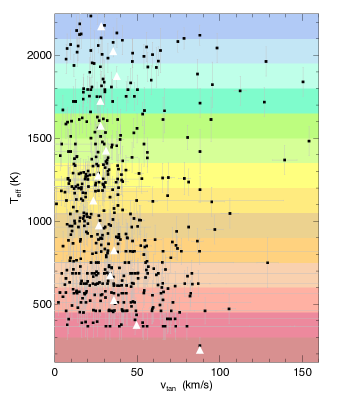
Figure 31: Tangential velocities plotted against effective temperature for L, T and Y dwarfs in the 20-pc census. Only those objects having parallax measurements with uncertainties $<$12.5% are shown. Individual objects are shown as black squares and the median $v_{tan}$ values in each 150K bin are shown as white triangles.

10 Conclusions

Our results, which use the final trigonometric parallaxes we have measured using Spitzer, confirm the result of Kirkpatrick et al. (2019) that the 20-pc brown dwarf portion of the mass function, which is based here on 525 L through Y dwarfs, can be best described as a power law with an exponent of $\alpha=0.6{\pm}0.1$. We have not yet, however, extended this analysis to higher masses to investigate how the mass function behaves over the entire mass range within 20 pc. Earlier analyses have indicated that the higher mass portion can be described as a two-part power law (Kroupa et al. 2013) or log-normal form (Chabrier 2003b). New data, particularly data from Gaia DR2 and subsequent releases can be used to refine our knowledge of the A through M dwarfs (and white dwarfs) with the 20-pc census as well as providing important astrometric information to help identify companions to those stars. Developing a database containing all knowledge of our stellar and substellar neighbors within this volume will enable us to explore the individual-object mass function with unprecedented detail.

Our results have also shown that the cutoff mass for star formation, is constrained to be lower than ${\sim}10M_{Jup}$ and that analysis of young moving group members over a wider sample likely constrains this value to ${\sim}5M_{Jup}$. Obtaining a more solid value for the cutoff mass requires volume-complete subsets of a substantial number of Y dwarfs colder than 450K, and particularly below $\sim$350K, a regime in which we have only one confirmed Y dwarf. Although WISE has provided a trove of Y dwarf discoveries, probing a substantial volume colder than $\sim$350K may require other resources. One such resource currently being planned is the Near Earth Object Surveyor (formerly called NEOCam) that is due to launch in 2025. As discussed in Kirkpatrick et al. (2019b), NEO Surveyor will cover 64% of the celestial sphere in two bands, NC1 and NC2, that cover wavelengths of 4.0-5.2 $\mu$m and 6.0-10.0 $\mu$m. Portions of the sky will be repeatedly scanned during their 75-day visibility windows then scanned again roughly 215 days later when the next visibility window opens. The mission, although planned for five years, has a design lifetime of twelve years.

The absolute NC1 fluxes of 350K Y dwarf and a 250K Y dwarf are 103 $\mu$Jy and 26 $\mu$Jy, respectively. The use of image differencing for high-motion objects in NEO Surveyor data will theoretically allow us to achieve single-epoch S/N=5 sensitivities of $\sim$4 $\mu$Jy at NC1, thereby greatly increasing the distances to which we can detect these coldest brown dwarfs. However, NEO Surveyor is run through NASA’s Planetary Defense Coordination Office, so no funding is being provided for the additional processing needed for astrophysical studies. For a relatively small investment, NASA Astrophysics could realize the full potential of NEO Surveyor data for stellar astrophysical research, of which cold brown dwarf discovery would be a major beneficiary.

Appendix A Spectral Types, Astrometry, and Photometry for Systems

For systems in Tables 5, 6, 7, 8, 9, 10, and 11, we have collected spectroscopic, astrometric, and photometric data from both this paper and the literature. These data are listed in Table 17. The various sections of the table are described in detail below. Close binaries are generally entered as a single entry with joint photometry unless there are components of the multiple with spectral types earlier than L0. For a full accounting of individual L, T, and Y components within the 20-pc census, refer to Table 11.

A.1 Origin and Name

Column $T$ indicates the table(s) from which the source originates. Objects in the 20-pc census (Table 11) are indicated by "T". Users are encouraged to use this column rather than the parallax column if they wish to select the same set of objects that we included in our 20-pc census. Objects that are not listed in our 20-pc census (Table 11) but were nonetheless part of our Spitzer parallax program (Tables 5-7) are indicated by "P". Objects that are not from any of these tables but were part of our photometric or spectroscopic follow-up campaigns (Tables 8 and 9) are indicated by "F". Objects considered for the 20-pc census but ultimately not included (Table 10) are indicated by "C".

Column $ShortName$ gives the abbreviated prefix and suffix of the full source name. This prefix is generally the survey of origin, and the abbreviated suffix is the sexagesimal RA and Dec of the source in the form $hhmm{\pm}ddmm$. As examples, CWISEP J193518.59$-$154620.3 is denoted as CWISE 1935$-$1546, and PSO J149.0341$-$14.7857 is denoted as PSO 0956$-$1447. Exceptions are made for objects with common names like Gl 570D and LHS 2397aB, whose full names are used instead.

A.2 Spectral Types

Columns $SpO$ and $SpIR$ list the optical and near-infrared spectral types, respectively, if known. These are converted to a decimal scale, and any qualifying criteria such as "pec", "$\beta$", and "sd" are dropped. The convention for the decimal scale is L0 = 0.0, T0 = 10.0, and Y0 = 20.0. As examples, an object with a spectral type of sdT8 is given as 18.0, and one with a type of L7: VL-G is given as 7.0. The two objects listed in Table 11 with types of "extremely red" in Mace et al. (2013) are given in this table as 9.5. Column $SpAd$ is the adopted spectral type, which is the same as $SpIR$ if that value is not null; otherwise, it is the same as $SpO$. If both of those quantities are null, a spectral type estimate is given. A few objects, however, have null values for $SpAd$, and these are objects believed to be background interlopers and not brown dwarfs.

The source of the spectral type is given in column $OI$. An explanation of the double-letter code for this column can be found in the table comments.

A.3 Astrometric Data

Columns $\varpi_{abs}$, $\mu_{\alpha}$, and $\mu_{\delta}$ list the best measured trigonometric parallax and proper motion values in RA and Dec. The "best" astrometry is simply that data set with the smallest quoted uncertainty in the parallax or, for objects lacking a parallax measurement, the data set with the smallest quoted uncertainty in the total proper motion. All parallaxes are given on the absolute reference grid; data from Tinney et al. (2003) and Tinney et al. (2014), along with USNO data from Kirkpatrick et al. (2019), were converted from relative to absolute as described in section 8 of Kirkpatrick et al. (2019). The values listed for proper motion are a mixture of relative and absolute measurements. Readers are encouraged to cite the source of those values if this distinction is important for their research.

The source of the astrometry is given in column $AS$. An explanation of the single-letter code for this column can be found in the table comments.

A.4 $JHK$ Photometry

Column $J_{MKO}$ lists $J$-band photometry on the MKO system, $J_{2MASS}$ lists $J$-band photometry one the 2MASS system, $H$ lists $H$-band photometry on either the MKO or 2MASS system, $K_{MKO}$ lists $K$-band photometry on the MKO system, and $K_{S(2MASS)}$ lists $K_{S}$-band photometry on the 2MASS system. See section 5.1.1 for details. Photometric values listed without corresponding errors are magnitude limits.

The source of the photometry is given in column $PhotS$. An explanation of the five-letter code for this column can be found in the table comments.

A.5 CatWISE2020 Data

Columns $RA\_C2$, $Dec\_C2$, $pmra\_C2$, $pmdec\_C2$, $W1mag\_C2$, $W2mag\_C2$, and $par\_C2$ contain astrometric information from the CatWISE2020 Catalog and Reject Table (Marocco et al. 2020b). The first two columns are the J2000 equinox RA and Dec positions from the moving-object solution at epoch MJD 57170.0, the next two columns are the measured proper motion and their uncertainties in RA and Dec, the next two columns are the moving-object PSF-fit photometry in WISE bands W1 and W2, and the final column is a crude measurement of the object’s parallax (called par_pm in the documentation).

The source of the CatWISE2020 data is given in column $C2S$. Upper-case "C2" refers to the Catalog and lower-case "c2" refers to the Reject Table.

A.6 AllWISE Data

Columns $W1mag$, $W2mag$, and $W3mag$ provide stationary-object PSF-fit measurements (primarily from AllWISE) in WISE bands W1, W2, and W3. These are provided for two reasons. First, CatWISE2020 does not provide any W3 data, since this band was not available for the post-cryogenic phases of the WISE and NEOWISE missions. Second, the short, six-month time baseline of AllWISE means that this stationary-object photometry should be robust for all sources except those of exceptionally large motion, and thus the W1 and W2 photometry can be compared to the moving-object photometry from CatWISE2020 to provide another photometric check.

The source of the stationary-object photometry is given in column $WS$. In most cases, this is the AllWISE Source Catalog or Reject Table. Some sources, however, were not detected until crowdsource (Schlafly et al. 2018) was used on the unWISE images underlying the CatWISE2020 processing. In this case, the stationary-object W1 and W2 photometry from CatWISE2020 is listed instead.

A.7 Spitzer Data

Columns $ch1mag$ and $ch2mag$ provide the Spitzer channel 1 (3.6 $\mu$m) and channel 2 (4.5$\mu$m) photometry. The source of this photometry is given in column $SS$, the single-character code for which is described in the table comments.

A.8 Note and Full Designation

Column $Note$ lists a one-letter code indicating whether the object is an unresolved multiple (M); a young, low-gravity object (Y), or an old, subdwarf (S). Column $FullName$ gives the full discovery designation of the system.

=65mm

Table 17: Amassed Spectroscopic, Astrometric, and Photometric Data for Objects Listed in Tables 5, 6, 7, 8, 9, 10, and 11

T	Name	SpO	SpIR	SpAd	OI	$\varpi_{abs}$	$\mu_{\alpha}$	$\mu_{\delta}$	AS	$J_{MKO}$	$J_{2MASS}$	$H$	$K_{MKO}$	$K_{S(2MASS)}$	PhotS	RA_C2	Dec_C2	…
						(mas)	(mas/yr)	(mas/yr)		(mag)	(mag)	(mag)	(mag)	(mag)		(deg)	(deg)
(1)	(2)	(3)	(4)	(5)	(6)	(7)	(8)	(9)	(10)	(11)	(12)	(13)	(14)	(15)	(16)	(17)	(18)	(19)
T	SDSS 0000+2554	15.0	14.5	14.5	TT	70.8 $\pm$ 1.9	$-$19.1 $\pm$ 1.5	126.7 $\pm$ 1.3	D	14.85$\pm$0.01	15.06$\pm$0.04	14.73$\pm$0.07	14.82$\pm$0.03	14.84$\pm$0.12	U22D2	0.0563043	25.9054854
T	GJ 1001BC	5.0	5.0	5.0	kT	82.0946$\pm$ 0.3768	671.09$\pm$ 0.35	$-$1498.16$\pm$ 0.51	G	12.98$\pm$0.01	13.11$\pm$0.02	12.06$\pm$0.03	$\cdots$	11.39$\pm$0.01	V22-V	1.1491771	$-$40.7415963
T	WISE 0005+3737	$\cdots$	19.0	19.0	-T	126.9 $\pm$ 2.1	997.3 $\pm$ 1.0	$-$271.6 $\pm$ 1.0	T	17.58$\pm$0.04	$\cdots$	17.98$\pm$0.02	$\cdots$	16.28$\pm$0.31	U-k-2	1.3250452	37.6219054
T	2MASS 0014$-$4844	2.5	2.5	2.5	TT	50.1064$\pm$ 0.3898	870.72$\pm$ 0.27	281.46$\pm$ 0.43	G	13.91$\pm$0.01	14.05$\pm$0.04	13.26$\pm$0.01	$\cdots$	12.78$\pm$0.01	V2V-V	3.7386552	$-$48.7367024
T	WISE 0015$-$4615	$\cdots$	18.0	18.0	-T	75.2 $\pm$ 2.4	413.4 $\pm$ 1.1	$-$687.8 $\pm$ 1.0	T	17.67$\pm$0.02	$\cdots$	17.91$\pm$0.07	$\cdots$	$\cdots$	V-V–	3.7755685	$-$46.2558784
T	2MASS 0015+3516	2.0	1.0	1.0	TT	58.6085$\pm$ 0.3664	55.17$\pm$ 0.45	$-$257.09$\pm$ 0.28	G	13.71$\pm$0.01	13.88$\pm$0.03	12.89$\pm$0.04	$\cdots$	12.26$\pm$0.02	UKK-2	3.9368016	35.2663391

Note. — Only a portion of the table’s rows and columns is shown here. The full table is available from the journal in machine-readable format.

Note. — References for OI, where the reference for the optical (O) spectral type is given as the first character and that for the near-infrared (I) spectral type is given as the second character: (a) Albert et al. 2011, (A) Thompson et al. 2013, (b) Burningham et al. 2010, (B) Burgasser, et al. 2010b, (c) Cushing et al. 2011, (C) Cushing et al. 2018, (d) Kirkpatrick et al. 2012, (D) Kirkpatrick et al. 2000, (e) Martin et al. 2018, (E) Reid et al. 2001b, (f) Kirkpatrick et al. 2010, (F) Faherty et al. 2014, (g) Burgasser et al. 2006, (G) Bardalez Gagliuffi, et al. 2014, (h) Hawley, et al. 2002, (H) Dhital et al. 2011, (i) Chiu et al. 2006, (I) Koen, et al. 2017, (J) Kirkpatrick et al. 1999, (j) Kirkpatrick et al. 2008, (k) Kirkpatrick et al. 2001, (K) Kirkpatrick et al. 2011, (l) Kendall et al. 2007, (L) Kendall et al. 2003, (m) Artigau et al. 2011, (M) Mace et al. 2013, (n) Scholz et al. 2003, (N) King et al. 2010, (p) Potter, et al. 2002, (P) Pineda et al. 2016, (q) Gizis 2002, (Q) Cruz, et al. 2007, (r) Reid et al. 2008, (R) Reid, et al. 2006, (s) Schneider, et al. 2014, (S) Schneider et al. 2015, (t) Tinney et al. 2018, (T) See Tables 9-12 in this paper for references, (u) Burningham et al. 2013, (U) Burgasser 2007, (v) Schneider et al. 2017, (V) Kirkpatrick et al. 2016, (w) Kendall, et al. 2004, (W) Best et al. 2013, (X) Burgasser et al. 2003d, (x) Thorstensen & Kirkpatrick 2003, (y) Deacon et al. 2014, (Y) Reylé et al. 2014, (z) Burgasser et al. 2010, (Z) Fan, et al. 2000.

Note. — References for AS, the source of the astrometric data: (A) Dahn et al. 2002, (b) Burgasser et al. 2008a, (B) Bartlett et al. 2017, (c) CatWISE2020 Catalog, (C) Tinney et al. 2014, (d) Dahn et al. 2017, (D) Dupuy & Liu 2012, (E) Dupuy et al. 2019, (F) Faherty et al. 2012, (G) Gaia DR2 - quoted astrometry is for the actual source listed, (g) Gaia DR2 - quoted astrometry is that of the brighter primary in the system, (J) Kirkpatrick et al. 2011, (H) Hipparcos - van Leeuwen 2007, (K) Kirkpatrick et al. 2019 for NTT and UKIRT parallaxes, (k) Kirkpatrick et al. 2019 for USNO parallaxes, (l) Leggett et al. 2012, (L) Liu et al. 2016, (m) Manjavacas et al. 2013, (M) Marocco et al. 2010, (r) Smart, priv. comm., (R) Smart et al. 2018, (S) Casewell et al. 2008, (s) Smart et al. 2013, (t) Tinney et al. 2003, (T) This paper, (V) Vrba et al. 2004, (W) Best et al. 2020, (z) Dupuy et al. 2020, (Z) Lazorenko, & Sahlmann 2018.

Note. — References for PhotS, the source of the $J,H,K$ photometry: (2) 2MASS Skrutskie et al. 2006, (a) Meisner et al. 2020a, (A) Meisner et al. 2020b, (b) Bardalez Gagliuffi et al. 2020: Note that the HST F125W magnitude limit for WISE 0830+2837 is used as its value for $J_{MKO}$, (B) Bigelow/2MASS, (c) Boccaletti et al. 2003, (C) CTIO-4m/NEWFIRM, (d) Kirkpatrick et al. 2012, (D) Database of Ultracool Parallaxes as of 2020 April: Dupuy & Liu 2012, Dupuy & Kraus 2013, and Liu et al. 2016, (e) Martin et al. 2018, (E) McElwain & Burgasser 2006, (f) Faherty et al. 2012, (F) Freed et al. 2003, (g) Mamajek et al. 2018, (G) Gemini-South/FLAMINGOS2, (h) Pinfield et al. 2014b, (H) Pinfield et al. 2014a, (i) Ireland et al. 2008, (I) Dupuy et al. 2019, (j) Janson et al. 2011, (J) Faherty et al. 2014b, (k) Kirkpatrick et al. 2019, (K) Kirkpatrick et al. 2011, (m) Mace et al. 2013, (M) Magellan/PANIC, (p) PAIRITEL, (P) Palomar/WIRC, (q) Dhital et al. 2011, (Q) Deacon et al. 2017a, (r) Deacon et al. 2012b, (s) Schneider et al. 2015, (S) SOAR/OSIRIS, (t) Tinney et al. 2014, (T) Thompson et al. 2013, (u) ULAS, UGPS, or UGCS, (U) UHS, (v) VVV, (V) VHS, (w) Wright et al. 2013, (W) Best et al. 2020.

Note. — References for C2S, the source of the CatWISE2020 data: (C2) CatWISE2020 Catalog, (c2) CatWISE2020 Reject Table.

Note. — References for WS, the source of the WISE photometry: (AW) AllWISE Source Catalog, (aw) AllWISE Reject Table, (C2) CatWISE2020 Catalog, (c2) CatWISE2020 Reject Table.

Note. — References for SS, the source of the Spitzer photometry: (0) This paper, (f) Marocco et al. 2020, (F) Filippazzo, et al. 2015, (K) Kirkpatrick et al. 2019, (L) Leggett et al. 2007, (M) Meisner et al. 2020a, (m) Meisner et al. 2020b, (P) Patten et al. 2006, (S) Metchev et al. 2015.

References

- Aberasturi et al. (2014) Aberasturi, M., Burgasser, A. J., Mora, A., et al. 2014, AJ, 148, 129
- Aberasturi et al. (2011) Aberasturi, M., Solano, E., & Martín, E. L. 2011, A&A, 534, L7.
- Adams et al. (1926) Adams, W. S., Joy, A. H., & Humason, M. L. 1926, ApJ, 64, 225
- Adams & Kohlschütter (1914) Adams, W. S., & Kohlschütter, A. 1914, Contributions from the Mount Wilson Observatory / Carnegie Institution of Washington, 79, 1
- Adams (1913) Adams, W. S. 1913, PASP, 25, 258
- Aganze et al. (2016) Aganze, C., Burgasser, A. J., Faherty, J. K., et al. 2016, AJ, 151, 46
- Albert et al. (2011) Albert, L., Artigau, É., Delorme, P., et al. 2011, AJ, 141, 203
- Allen et al. (2005) Allen, P. R., Koerner, D. W., Reid, I. N., & Trilling, D. E. 2005, ApJ, 625, 385
- Allers & Liu (2013) Allers, K. N. & Liu, M. C. 2013, ApJ, 772, 79.
- Andrei et al. (2011) Andrei, A. H., Smart, R. L., Penna, J. L., et al. 2011, AJ, 141, 54.
- Artigau et al. (2011) Artigau, É., Lafrenière, D., Doyon, R., et al. 2011, ApJ, 739, 48.
- Artigau et al. (2010) Artigau, É., Radigan, J., Folkes, S., et al. 2010, ApJ, 718, L38
- Artigau et al. (2006) Artigau, É., Doyon, R., Lafrenière, D., et al. 2006, ApJ, 651, L57.
- Baraffe et al. (2003) Baraffe, I., Chabrier, G., Barman, T. S., Allard, F., & Hauschildt, P. H. 2003, A&A, 402, 701