Multi-task Learning for Human Settlement Extent Regression and Local Climate Zone Classification

Abstract

This work has been accepted by IEEE GRSL for publication. Human Settlement Extent (HSE) and Local Climate Zone (LCZ) maps are both essential sources, e.g., for sustainable urban development and Urban Heat Island (UHI) studies. Remote sensing (RS)- and deep learning (DL)-based classification approaches play a significant role by providing the potential for global mapping. However, most of the efforts only focus on one of the two schemes, usually on a specific scale. This leads to unnecessary redundancies, since the learned features could be leveraged for both of these related tasks. In this letter, the concept of multi-task learning (MTL) is introduced to HSE regression and LCZ classification for the first time. We propose a MTL framework and develop an end-to-end Convolutional Neural Network (CNN), which consists of a backbone network for shared feature learning, attention modules for task-specific feature learning, and a weighting strategy for balancing the two tasks. We additionally propose to exploit HSE predictions as a prior for LCZ classification to enhance the accuracy. The MTL approach was extensively tested with Sentinel-2 data of 13 cities across the world. The results demonstrate that the framework is able to provide a competitive solution for both tasks.

I Introduction

Two important tasks in urban mapping are distinguishing urban areas from non-urban background and characterizing intra-urban heterogeneity. HSE and LCZs are two schemes for the respective representations. HSE density, indicating the portion of buildings, roads, and other man-made structures in an area (e.g., a pixel), depicts the human footprint on Earth. By contrast, the LCZ scheme, originally proposed for UHI studies, includes 17 classes for detailed land cover (LC) classification [1], and is universally applicable. Up-to-date, detailed, and accurate worldwide information on HSE and LCZ can provide support for evidence-based decision making for various applications e.g., global climate science [2, 3].

DL-based approaches for LC classification have been attracting much attention due to their proven predictive power, and end-to-end learning abilities of complex feature representations. CNNs, in particular Fully Convolutional Networks (FCNs), have been successfully applied to many RS-based image classification and segmentation tasks [4]. In this study, we draw upon these successes by applying DL-based semantic segmentation methods to LC mapping. However, LC mapping, particularly LCZ classification over a large scale remains challenging due to the large intra-class variability of spectral signatures, which stems from variations in physical and cultural environmental characteristics across the world and a limited amount of reference data [5].

This challenge and the lack of fully automated approaches to it motivate our investigations into DL models with a higher generalization ability for LC mapping. As already suggested by the definition of the two schemes, prior work also indicated that HSE and LCZs have close correspondence for different study areas [1, 6]. To exploit the complementary nature of the HSE regression and LCZ classification tasks, we propose a MTL framework to jointly predict HSE and LCZs, considering that MTL has been shown to be a powerful technique for improving model generalization by leveraging domain knowledge of related complementary tasks [7, 8]. In this work, we present a feature-based MTL system that mainly consists of a shared backbone network to capture a common representation for both HSE regression and LCZ classification, and soft-attention modules to adaptively select task-specific features. By jointly learning both tasks, we aim to boost the prediction performance over that achieved by a single, task-specific network.

II Methodology

II-A A General MTL Framework for LC Mapping on Different Scales

In the definition of LCZ, one important factor to consider is the ratio of impervious surface and buildings, which indicates that the HSE density affects the categorization of an area in the LCZ scheme. Additionally, HSE regression and LCZ classification prioritize spatial and semantic resolution in a complementary manner. The LCZ scheme places emphasis on the characterization of urban morphology with 17 classes (for a relatively large neighboring area, e.g., $100\text{\,}\mathrm{m}$), while the HSE density contains fewer semantic details but features a higher spatial resolution (e.g., $20\text{\,}\mathrm{m}$). The complementary relationship, when appropriately exploited, is expected to support the learning process of each task and improves the efficient usage of available training data. This will potentially lead to faster convergence during training, higher accuracy for both tasks compared to single-task models, and reduced production time as both tasks can occur in parallel. To this end, a generalized MTL framework, illustrated in Fig. 1, is proposed, which consists of the following four primary components.

• A backbone network for shared, general feature learning at the early stage. It can be implemented as state-of-the-art CNN architectures, such as residual neural networks. Compared to natural images, e.g., photographs typically used in computer vision experiments, the resolution of Sentinel-2 imagery is low. Hence, pooling should be less used within the backbone network to retain the spatial resolution and the information of the pixel values.

• Task-specific network branches for dedicated feature learning to adaptively select features from the common representations and further learn specific and high-level features for the individual tasks. They can be implemented as convolutional operations, attention modules or “Squeeze-and-Excitation” blocks [9].

• Decoder modules to recover the required resolution of predictions. They can be implemented as transposed convolutions or upsampling layers. To retain clear boundaries, low level features might need to be considered, e.g., via skip connections.

• Modules to exploit task relation. The reference of one task can be employed as prior information to guide the prediction of the other task. In this way, consistent and accurate predictions are encouraged in the MTL framework.

Figure 1: A general MTL framework for HSE density regression and LCZ classification, consisting of a backbone network, task-specific network branches, and decoder modules. The inputs for network training are images and corresponding reference labels for each task.

II-B Implementation of the MTL Framework

One implementation of the proposed MTL framework is illustrated in Fig. 2, which consists of a backbone network (including convolutional layers and pooling layers) followed by two branches for HSE regression and LCZ classification. Each of the two branches begins with an attention module, implemented as Convolutional Block Attention Modules (CBAMs), for an adaptive selection and learning of task-specific representations [10]. All $3\times 3$ convolutional layers make use of separable convolution operations for the sake of efficiency. A kernel size of $2\times 2$ with a stride of 2 was used for the pooling layers, decreasing the size of feature maps by half. Maximum and average pooling layers were used together for abstracting learned features within the architecture to preserve sufficient features. The final output of both tasks was decided based on the desired ground sampling distance (GSD) of the respective products. To avoid overfitting during training, one and two drop-out layers with a dropout rate of 0.1 were utilized in the HSE and LCZ branches (omitted in the illustration).

For the HSE regression task, the last layer was activated with a sigmoid function, and the mean absolute error (MAE) was used as a loss function to consider potential noise in the reference data. Considering that there are more samples with no or few human settlements in our dataset, a relatively high weight was assigned to samples with dense human settlements to deal with the imbalance problem. The sample weight was decided based on: $e^{y_{\text{HSE}}}$, where ${y_{\text{HSE}}}\in[0,1]$ is the reference label for HSE density.

For the LCZ classification task, predicted softmax probabilities from intermediate lower-level, features were also used for the loss calculation, in addition to the final prediction. Specifically, for each input patch, three $1\times 1$ convolutional and softmax layers were used to independently predict three results using intermediate features (indicated by dashed gray lines in Fig. 2). This is to fully exploit the features at different levels for the elaborate LCZ scheme, which requires a diversity of representations to distinguish the 17 distinct LCZ classes. Together with the result produced by the final layers (represented by a solid green line in Fig. 2), these four results were upsampled to the same size as the prepared reference label patches. All four patches of predicted softmax probabilities were averaged into one final patch for the loss calculation of the LCZ branch using a softmax cross entropy loss.

The final MTL loss, which was used to train the MTL network, was a combination of the two single-task losses from the HSE regression task and the LCZ classification tasks.

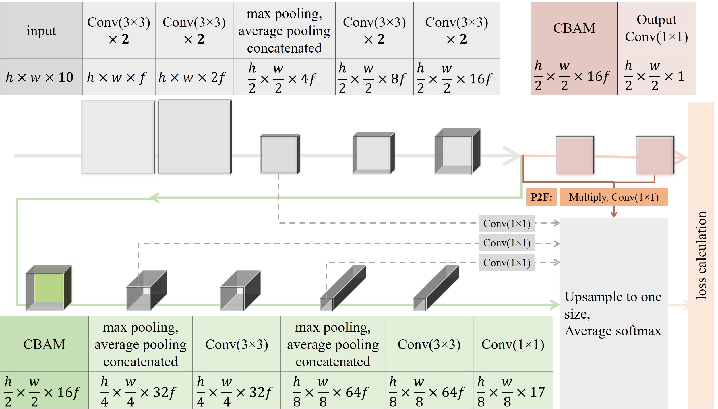
Figure 2: Illustration of the implemented MTL CNN architecture for HSE regression and LCZ classification. The backbone network consists of two convolutional blocks, one pooling block, and two more convolutional blocks. The two task-specific network branches are indicated by two different colors. The description of each layer and the size of inputs, feature maps, and outputs are listed along with the operations. $h$ and $w$ are height and width of the input patch, and $f$ is the number of feature maps from the first layer.

II-C Predictions as Features (P2F)

HSE density and LCZs do not merely share similar properties, which motivated the implicit exploitation via a MTL framework. The HSE density is, furthermore, explicitly affecting the categorization of a subset of LCZs. For instance, an area with a high HSE density cannot belong to a LCZ class that corresponds to natural areas, e.g., dense trees. Following this principle, a module called predictions as features (P2F) was designed to exploit this prior knowledge within our framework, the implementation of which was inspired by Kohl et al. [11]. The main idea is to use the HSE predictions as a prior for the classification of LCZs, as illustrated in Figs. 1 and 2. Specifically, the HSE reference was multiplied with the intermediate features, resulting in processed feature maps. These feature maps were used to get an additional prediction of LCZ classes, providing an additional output of the LCZ branch.

The P2F module was used in a different manner during training and test time. Since reference labels for HSE were available at training-time, they can be utilized as the prior for the prediction of LCZs. At test-time, the prior was predictions of the HSE regression branch in the multi-task network, as indicated in Fig. 1. Thus, the system still solely relies on a single image as its input at test-time, while making use of the available ground-truth data during training. The quality of HSE predictions is expected to be useful for the P2F concept as satisfying HSE mapping results have been achieved using deep CNNs [12].

II-D Dynamically Balancing Task Weights

One of the challenges in MTL is to balance the involved tasks, which is most commonly implemented by weighting each individual loss in the multi-task loss, subject to optimization. Simply summing the contributing losses, assuming equal task weights of 1, is not sufficient in most cases, as this not only implies equal importance of the tasks but also that single-task losses produce values in the same order of magnitude. Manually tuning such weights as hyper-parameters, however, is tedious. Hence, approaches to automatically and dynamically determine them are desired and have been investigated in the literature [13, 14].

We implemented an approach to weighting the HSE regression and LCZ classification tasks based on homoscedastic uncertainty, introduced by [13]. Specifically, we optimize a multi-task loss function

$$\mathcal{L}_{\text{MT}}(\mathbf{W}_{\text{HSE/LCZ}},\sigma_{\text{HSE/LCZ}})= \frac{1}{2\sigma_{\text{HSE}}^{2}}\mathcal{L}_{\text{HSE}}(\mathbf{W}_{\text{HSE}})$$

$$+\frac{1}{\sigma_{\text{LCZ}}^{2}}\mathcal{L}_{\text{LCZ}}(\mathbf{W}_{\text{LCZ}})$$

$$+\log{\sigma_{\text{HSE}}}+\log{\sigma_{\text{LCZ}}}$$ (1)

where $\mathcal{L}_{\text{HSE/LCZ}}$ is the MAE and cross entropy loss for HSE regression and LCZ classification task, respectively, $\mathbf{W}_{\text{HSE/LCZ}}$ are the trainable parameters from the network layers of respective branch, and $\sigma_{\text{HSE/LCZ}}$ are weighting parameters that control the contribution of the individual tasks. The variables for the input and reference data, $\mathbf{X}$, $\mathbf{Y}$, are omitted in the above equation. The regularization terms $\log{\sigma_{\text{HSE/LCZ}}}$ prevent trivial solutions for $\sigma_{\text{HSE/LCZ}}\to\pm\infty$. We optimized the weighting terms along with the network parameters as $s_{\text{HSE/LCZ}}:=\log{\sigma_{\text{HSE/LCZ}}^{2}}$ due to numerical stability [13].

III Experimental Evaluation

III-A Dataset for Training

A dataset was prepared to assess the potential of the proposed MTL framework, including Sentinel-2 image patches from three seasons (spring, summer, and autumn 2017) and annotations for both tasks, i.e., HSE density percentage and LCZ labels.

The imagery was processed in accordance with previous work [12] using the five European cities, namely Berlin, Lisbon, Madrid, Milan, and Paris as study areas. Annotations for the HSE density regression are from “High Resolution Layer Imperviousness 2015,” using continuous values indicating the percentage of each pixel covered by HSE, with a GSD of $20\text{\,}\mathrm{m}$ [15, 16]. Additionally, pixel-wise LCZ labels were prepared for each sample, using the reference from the WUDPAT project [17], with an original GSD of $100\text{\,}\mathrm{m}$. It was upsampled to $10\text{\,}\mathrm{m}$ to match the co-registered image patches during the training period. At test time, LCZ predictions with a GSD of $100\text{\,}\mathrm{m}$ were produced to be consistent with state-of-the-art LCZ-related studies. The number of spatially disjoined training and validation patches was 75116 and 24706, respectively, with a size of $128\times 128$ px.

III-B Test Data and Accuracy Assessment

For assessment of the HSE regression task, two test datasets were used. The first one covers three test scenes in Europe, namely Amsterdam, London, and Munich and was prepared in the same way as the training data. Hence, the HSE density data is available for this test dataset. The MAE is used as a metric when tested on this dataset. To test the HSE regression performance on a large scale, a qualitative evaluation in comparison to HR images was carried out. Furthermore, the predicted results were aggregated into binary labels and tested against manually annotated ground checking points, as introduced by Qiu et al. [12], which are uniformly distributed over ten scenes across the world. Metrics for evaluation include Kappa, average accuracy (AA), recall, and F-Score of HSE. This evaluation procedure, with two test datasets, can provide an estimation of the generalization ability of the proposed MTL approach, which was trained on data from Europe exclusively.

To assess the LCZ classification task, we utilized the same ten worldwide scenes as the HSE regression, with reference labels from the So2Sat LCZ42 dataset, which was processed by polygon shrinking and class balancing after labelling [18]. The number of test samples for each scene is shown in Fig. 3. In addition to overall accuracy (OA), Kappa, and AA, Weighted accuracy (WA) was used by assigning different penalties to different mistakes.

Figure 3: Sample number of each test scene for LCZ classification assessment.

III-C Hyper-Parameter Settings

All models in this study were implemented in Keras for TensorFlow and trained from scratch. Basic hyper-parameters include a batch size of 8 and an initial learning rate of 0.002 for the Nesterov Adam optimizer. The learning rate was decreased by 0.25 after every two epochs. To control the training time and avoid overfitting, early stopping was implemented with the validation loss as the monitored metric with a patience of 10 epochs.

III-D Results for Different Settings

Table I presents evaluation results for HSE regression and LCZ classification over both test sets. In addition to single- and multi-task training, different strategies of feature exploitation and task weighting are also compared.

TABLE I: Comparison of results from different approaches tested within and outside Europe. The values were averaged over three and ten test areas for the European and the global test set. For each metric, the top two best results were marked in bold.

Configuration	European Test Set					Global Test Set
	HSE Density	HSE Aggregated				HSE Aggregated				LCZ
	MAE	Kappa	AA	Recall	F	Kappa	AA	Recall	F	OA	Kappa	AA	WA
Single-Task HSE	$4.24$	$0.76$	$0.92$	$0.91$	$0.94$	$0.78$	$0.8879$	$0.9302$	$0.89$	—	—	—	—
Single-Task LCZ	—	—	—	—	—	—	—	—	—	$0.4784$	$0.41$	$0.3413$	$0.8543$
Multi-Task (1:1, CBAM)	$4.55$	$0.69$	$0.90$	$0.86$	$0.91$	$0.77$	$0.8855$	$0.9445$	$0.89$	$0.4951$	$0.42$	$0.3379$	$0.8773$
Multi-Task (1:1, CBAM, P2F)	$4.39$	$0.71$	$0.90$	$0.87$	$0.92$	$0.78$	$0.8895$	$0.9221$	$0.90$	$0.4397$	$0.37$	$0.3095$	$0.8173$
Multi-Task (learned weights, CBAM)	$4.49$	$0.76$	$0.91$	$0.91$	$0.94$	$0.80$	$0.8995$	$0.9182$	$0.90$	$0.4813$	$0.42$	$0.3609$	$0.8809$
Multi-Task (learned weights, P2F)	$4.14$	$0.77$	$0.92$	$0.92$	$0.95$	$0.81$	$0.9036$	$0.9238$	$0.91$	$0.4533$	$0.38$	$0.3169$	$0.8318$
Multi-Task (learned weights, CBAM, P2F)	$4.12$	$0.79$	$0.91$	$0.93$	$0.95$	$0.80$	$0.9004$	$0.9032$	$0.90$	$0.5011$	$0.44$	$0.3637$	$0.8813$

An illustration of the MTL predictions is presented in Fig. 4 for a test scene in New York City. Both HSE regression and LCZ classification results reflect the pattern of urban structures in the imagery, indicating a reasonable mapping result.

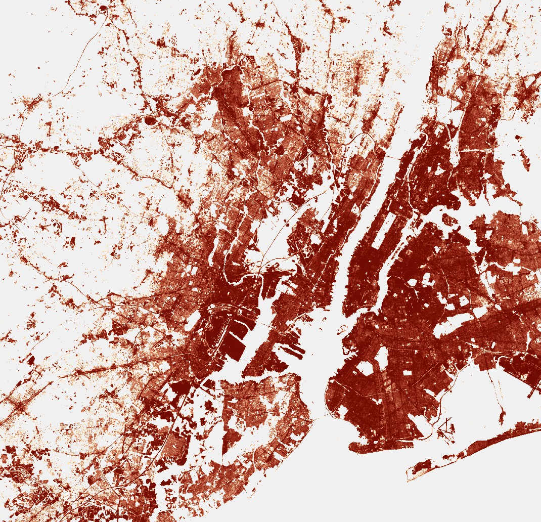
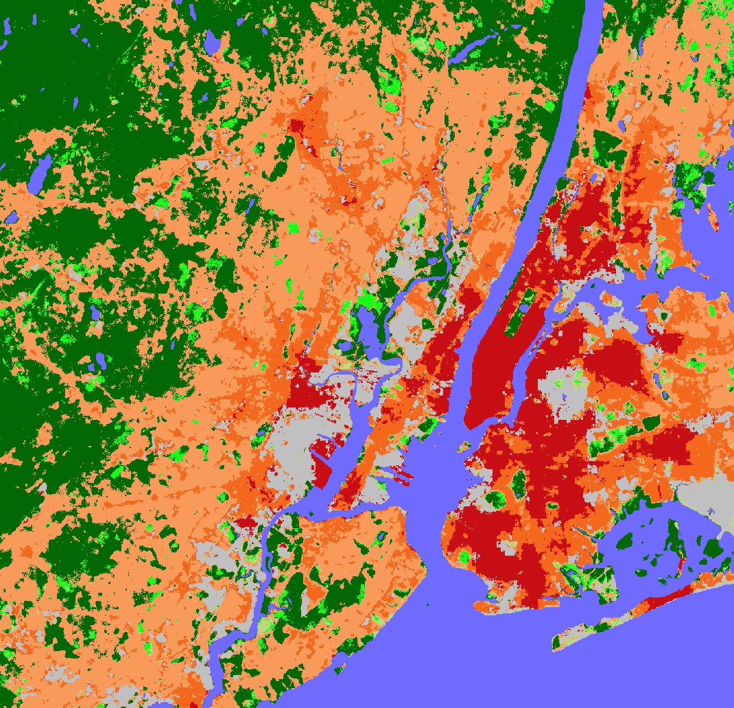
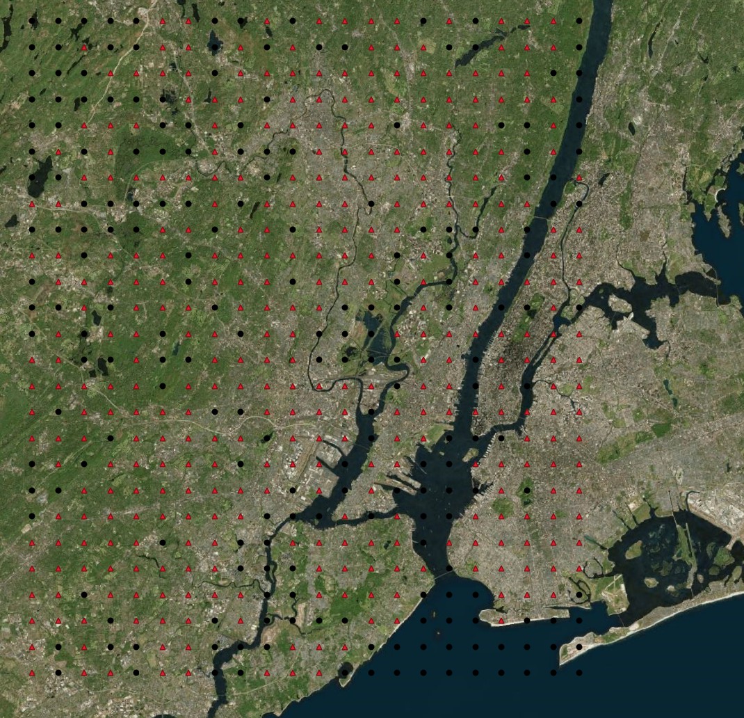
Figure 4: An illustration of joint prediction results in New York City (NYC), USA. From left to right are results of HSE regression and LCZ classification (with the same legend as Fig. 3), and HR image overlaid with reference points (red for HSE and black for non-HSE), respectively.

IV Discussion

IV-A Superiority of the Proposed MTL Approach

Joint prediction was able to provide benefits for both tasks, as analyzed in the following. Simply weighting the two contributing single-task losses equally ($1:1$) only resulted in a slight improvement for OA and Kappa in the LCZ classification task, as shown in Table I. When using the dynamically learned weights, the benefit became apparent, with AA being improved from 0.89 to 0.90 and from 0.34 to 0.36 for HSE and LCZ results. This shows that the dynamical weight learning strategy plays a positive role in the MTL performance.

The proposed strategy of using the HSE density predictions as features for LCZ classification, P2F, was able to additionally improve the effectiveness of the MTL configuration, providing best results among all investigated approaches for the LCZ classification task. This is an improvement over the basic approaches, such as single-task learning, with Kappa being improved from 0.41 to 0.44 and OA being improved from 0.478 to 0.50. This effect can be attributed to guidance from the HSE density mapping task. Intuitively, the candidate LCZ type of an area can be narrowed down when built-up areas were already detected in the HSE regression task. This piece of useful information from HSE regression can be leveraged for LCZ classification, leading to a further improvement over baseline MTL approaches. It can also be noted from Table I that P2F was not able to provide improvement when the task weights were $1:1$, which indicates the importance of an appropriate weighting strategy.

Task-specific feature learning modules, e.g., CBAMs utilized in the experiments, are important for gaining benefits within the MTL framework. This can be proved by comparing the results with and without CBAMs in Table I. All metrics for LCZ classification were worse when removing CBAMs from the MTL architecture. A possible reason is that HSE mapping and LCZ classification each require some different lower-level features, which cannot be satisfied in the absence of attention modules as a feature selection process. Another possible reason for the improved results from MTL is that multi-source reference data is used. This helps to learn more generalized features, and thus the model is less prone to overfitting, compared to single-task learning.

IV-B Quality of Current Mapping Results and Future Work

The achieved HSE regression results, representing continuous HSE density, provide richer information beyond a binary delineation of urban areas, such as the Global Urban Footprint (GUF), the Global Human Settlement (GHS) built-up grid, and our previous work [12]. Quantitatively, the accuracy is higher using the same checking points as a test set. Specifically, the AA, recall, and F-score of our previous binary HSE mapping results are 0.90, 0.91, and 0.91, respectively. All these metrics are beyond the state-of-the-art products when tested on the same 10 distinct scenes. For instance, AA of the GUF and the GHS built-up grid are 0.86 and 0.83. It should be noted, however, that the temporal gaps between the checking points and these products might play a role in this comparison.

As a proof of concept, reference data from only five European scenes was collected and used to train the MTL network. Still, the achieved LCZ classification results are promising over ten distinct test scenes across the world, demonstrating the capability for generalization and potential for further exploring this challenging task. The accuracy is reasonable when compared to state-of-the-art work using similar experimental settings, i.e., tested on completely unseen areas [5]. More accurate LCZ classification results can be expected if larger amounts of high-quality reference data are available in the future, as the LCZ reference might still contain errors, even after manual editing by expert annotators. Future work includes exploring the potential of MTL for more test scenes and longer time series to provide support for applications such as environmental management and monitoring.

V Conclusion

HSE density and LCZ maps are both vital for urban analysis. Based on the intuition that both tasks are highly correlated and might provide hints for each other, we proposed to jointly predict HSE density and LCZ labels via a MTL approach, and developed a MTL-based CNN to better leverage the complimentary features extracted from the input satellite imagery. We validated the proposed approach with extensive experiments using Sentinel-2 data in the context of large-scale urban analysis. This letter shows that related urban mapping tasks can be performed jointly for improved generalization ability of DL models.

References

- Stewart and Oke [2012] I. D. Stewart and T. R. Oke, “Local climate zones for urban temperature studies,” Bull. Am. Meteorol. Soc., vol. 93, no. 12, pp. 1879–1900, 2012.
- Corbane et al. [2017] C. Corbane, M. Pesaresi, P. Politis, V. Syrris et al., “Big earth data analytics on Sentinel-1 and Landsat imagery in support to global human settlements mapping,” Big Earth Data, vol. 1, no. 1-2, pp. 118–144, 2017.
- Esch et al. [2013] T. Esch, M. Marconcini, A. Felbier, A. Roth, W. Heldens, M. Huber, M. Schwinger, H. Taubenböck, A. Müller, and S. Dech, “Urban footprint processor—fully automated processing chain generating settlement masks from global data of the TanDEM-X mission,” IEEE Geosci. Remote Sens. Lett., vol. 10, no. 6, pp. 1617–1621, 2013.
- Zhang et al. [2019] C. Zhang, I. Sargent, X. Pan, H. Li, A. Gardiner, J. Hare, and P. M. Atkinson, “Joint deep learning for land cover and land use classification,” Remote Sens. Environ., vol. 221, pp. 173–187, 2019.
- Demuzere et al. [2019] M. Demuzere, B. Bechtel, and G. Mills, “Global transferability of local climate zone models,” Urban Clim., vol. 27, pp. 46–63, 2019.
- Bechtel et al. [2016] B. Bechtel, M. Pesaresi, L. See, G. Mills, J. Ching, P. Alexander, J. Feddema, A. Florczyk, and I. Stewart, “Towards consistent mapping of urban structures-global human settlement layer and local climate zones,” in XXIII ISPRS Congress, 2016, pp. 1371–1378.
- Ruder [2017] S. Ruder, “An overview of multi-task learning in deep neural networks,” arXiv preprint:1706.05098, 2017.
- Liebel et al. [2020] L. Liebel, K. Bittner, and M. Körner, “A generalized multi-task learning approach to stereo DSM filtering in urban areas,” ISPRS J. Photogramm. Remote Sens., vol. 166, pp. 213–227, 2020.
- Hu et al. [2018] J. Hu, L. Shen, and G. Sun, “Squeeze-and-excitation networks,” in Proc. IEEE CVPR, 2018, pp. 7132–7141.
- Woo et al. [2018] S. Woo, J. Park, J.-Y. Lee, and I. So Kweon, “Cbam: Convolutional block attention module,” in Proc. IEEE ECCV, 2018, pp. 3–19.
- Kohl et al. [2018] S. Kohl, B. Romera-Paredes, C. Meyer, J. De Fauw, J. R. Ledsam, K. Maier-Hein, S. A. Eslami, D. J. Rezende, and O. Ronneberger, “A probabilistic u-net for segmentation of ambiguous images,” in NeurIPS, 2018, pp. 6965–6975.
- Qiu et al. [2020] C. Qiu, M. Schmitt, C. Geiß, T.-H. K. Chen, and X. X. Zhu, “A framework for large-scale mapping of human settlement extent from sentinel-2 images via fully convolutional neural networks,” ISPRS J. Photogramm. Remote Sens., vol. 163, pp. 152 – 170, 2020.
- Kendall et al. [2018] A. Kendall, Y. Gal, and R. Cipolla, “Multi-task learning using uncertainty to weigh losses for scene geometry and semantics,” in Proc. IEEE CVPR, 2018, pp. 7482–7491.
- Guo et al. [2018] M. Guo, A. Haque, D.-A. Huang, S. Yeung, and L. Fei-Fei, “Dynamic task prioritization for multitask learning,” in Proc. IEEE ECCV, 2018, pp. 282–299.
- Langanke [2016] T. Langanke, “Copernicus land monitoring service – high resolution layer imperviousness: Product specifications document,” Copernicus team at EEA, 2016.
- [16] “Data source of the HSE reference,” https://land.copernicus.eu/pan-european/high-resolution-layers/imperviousness, accessed on: 2019-01-20.
- [17] “LCZ reference from WUDAPT project website,” http://www.wudapt.org/continental-lcz-maps/, accessed on: 2020-03-30.
- et al. [2020] X. X. Z. et al., “So2Sat LCZ42: A benchmark data set for the classification of global local climate zones,” IEEE Geoscience and Remote Sensing Magazine, vol. 8, no. 3, pp. 76–89, 2020.