Coronal heating problem solution by means
of axion origin photons

Abstract

In this paper we advocate for the idea that two seemingly unrelated mysteries with almost 90 year history – the nature of dark matter and the million-degree solar corona – may be but two sides of the same coin – the axions of dark matter born in the core of the Sun and photons of axion origin in the million-degree solar corona, whose modulations are controlled by the anticorrelated modulation of the asymmetric dark matter (ADM) density in the solar interior.

It is shown that the photons of axion origin, that are born in the almost empty magnetic flux tubes (with $B\sim 10^{7}~{}G$) near the tachocline and then pass through the photosphere to the corona, are the result of the solar corona heating variations, and thus, the Sun luminosity variations. Since the spectrum of the incident photons of axion origin is modulated by the frequency dependence of the cross-section, then, first, the energy distribution of the emitted axions is far from being a blackbody spectrum, and second, for a typical solar spectrum, the maximum of the differential axion flux occurs at the average axion energy is $\langle E_{a}/T\rangle\approx 4.4$ (Raffelt,1986). This means that the average energy of the photon of axion origin can generate a temperature of the order of $T_{a}\sim 1.11\cdot 10^{7}~{}K$ under certain conditions of coronal substances, which is close to the temperature $T_{core}\sim 1.55\cdot 10^{7}~{}K$ of the Sun core.

As a result, the free energy accumulated by the photons of axion origin in a magnetic field by means of degraded spectra due to multiple Compton scattering, is quickly released and converted into heat and plasma motion with a temperature of $\sim 4\cdot 10^{6}~{}K$ at maximum and $\sim 1.5\cdot 10^{6}~{}K$ at minimum of solar luminosity.

Since the photons of axion origin are the result of the Sun luminosity variations, then, unlike the self-excited dynamo, an unexpected but simple question arises: is there a dark matter chronometer hidden deep in the Sun core?

A unique result of our model is the fact that the periods, velocities and modulations of S-stars are the fundamental indicator of the modulation of the ADM halo density in the fundamental plane of the Galaxy center, which closely correlates with the density modulation of the baryon matter near the SMBH. If the modulations of the ADM halo at the GC lead to modulations of the ADM density on the surface of the Sun (through vertical density waves from the disk to the solar neighborhood), then there is an “experimental” anticorrelation identity between the indicators, e.g. the modulation of the ADM density in the solar interior and the number of sunspots. Therefore, this is also true for the modulation of the ADM density in the solar interior, which is directly related to the identical periods of S-star cycles and the sunspot cycles.

1 Introduction

A hypothetical pseudoscalar particle called axion is predicted by the theory related to solving the CP-invariance violation problem in QCD. The most important parameter determining the axion properties is the energy scale $f_{a}$ of the so-called U(1) Peccei-Quinn symmetry violation. It determines both the axion mass and the strength of its coupling to fermions and gauge bosons including photons. However, in spite of the numerous direct experiments, axions have not been discovered so far. Meanwhile, these experiments together with the astrophysical and cosmological limitations leave a rather narrow band for the permissible parameters of invisible axion (e.g. $10^{-6}eV\leqslant m_{a}\leqslant 10^{-2}eV$ [1, 2]), which is also a well-motivated cold dark matter (CDM) candidate in this mass region [1, 2].

Let us give some implications and extractions from the photon-axion oscillations theory which describes the process of the photon conversion into an axion and back under the constant magnetic field $B$ of the length $L$. It is easy to show [3, 4, 5, 6] that in the case of the negligible photon absorption coefficient ($\Gamma_{\gamma}\to 0$) and axions decay rate ($\Gamma_{a}\to 0$) the conversion probability is

$$P_{a\rightarrow\gamma}=\left(\Delta_{a\gamma}L\right)^{2}\sin^{2}\left(\frac{\Delta_{osc}L}{2}\right)\Big{/}\left(\frac{\Delta_{osc}L}{2}\right)^{2}\,,$$ (1)

where the oscillation wavenumber $\Delta_{osc}$ is given by

$$\Delta_{osc}^{2}=\left(\Delta_{pl}+\Delta_{Q,\perp}-\Delta_{a}\right)^{2}+4\Delta_{a\gamma}^{2}$$ (2)

while the mixing parameter $\Delta_{a\gamma}$, the axion-mass parameter $\Delta_{a}$, the refraction parameter $\Delta_{pl}$ and the QED dispersion parameter $\Delta_{Q,\perp}$ may be represented by the following expressions:

$$\Delta_{a\gamma}=\frac{g_{a\gamma}B}{2}=540\left(\frac{g_{a\gamma}}{10^{-10}GeV^{-1}}\right)\left(\frac{B}{1G}\right)~{}~{}pc^{-1}\,,$$ (3)

$$\Delta_{a}=\frac{m_{a}^{2}}{2E_{a}}=7.8\cdot 10^{-11}\left(\frac{m_{a}}{10^{-7}eV}\right)^{2}\left(\frac{10^{19}eV}{E_{a}}\right)~{}~{}pc^{-1}\,,$$ (4)

$$\Delta_{pl}=\frac{\omega^{2}_{pl}}{2E_{a}}=1.1\cdot 10^{-6}\left(\frac{n_{e}}{10^{11}cm^{-3}}\right)\left(\frac{10^{19}eV}{E_{a}}\right)~{}~{}pc^{-1},$$ (5)

$$\Delta_{Q,\perp}=\frac{m_{\gamma,\perp}^{2}}{2E_{a}}.$$ (6)

Here $g_{a\gamma}$ is the constant of axion coupling to photons; $B$ is the transverse magnetic field; $m_{a}$ and $E_{a}$ are the axion mass and energy; $\omega^{2}_{pl}=4\pi\alpha n_{e}/m_{e}$ is an effective photon mass in terms of the plasma frequency if the process does not take place in vacuum, $n_{e}$ is the electron density, $\alpha$ is the fine-structure constant, $m_{e}$ is the electron mass; $m_{\gamma,\perp}^{2}$ is the effective mass square of the transverse photon which arises due to interaction with the external magnetic field.

The conversion probability (1) is energy-independent, when $2\Delta_{a\gamma}\approx\Delta_{osc}$, i.e.

$$P_{a\rightarrow\gamma}\cong\sin^{2}\left(\Delta_{a\gamma}L\right)\,,$$ (7)

or whenever the oscillatory term in (1) is small ($\Delta_{osc}L/2\to 0$), implying the limiting coherent behavior

$$P_{a\rightarrow\gamma}\cong\left(\frac{g_{a\gamma}BL}{2}\right)^{2}\,.$$ (8)

It is worth noting that the oscillation length corresponding to (7) reads

$$L_{osc}=\frac{\pi}{\Delta_{a\gamma}}=\frac{2\pi}{g_{a\gamma}B}\cong 5.8\cdot 10^{-3}\left(\frac{10^{-10}GeV^{-1}}{g_{a\gamma}}\right)\left(\frac{1G}{B}\right)~{}pc$$ (9)

assuming a purely transverse field. In the case of the appropriate size $L$ of the region a complete transition between photons and axions is possible.

From now on we are interested in the energy-independent case (7) or (8) which plays the key role in determination of the parameters for the axion mechanism of Sun luminosity variations (the axion coupling constant to photons $g_{a\gamma}$, the transverse magnetic field $B$ of length $L$ and the axion mass $m_{a}$).

To estimate the hadron axion-photon coupling constant, we focus on the conversion probability

$$P_{a\rightarrow\gamma}=\frac{1}{4}\left(g_{a\gamma}B_{MS}L_{MS}\right)^{2}\sim 1,~{}~{}L_{MS}\equiv L_{osc}$$ (10)

where the complete conversion between photons and axions is possible by means of estimating the axion coupling constant to photons.

We showed a solution to the well-known problem of the Parker-Biermann cooling effect, which is determined by the nature of strong toroidal magnetic fields in tachocline (by the thermomagnetic Ettingshausen-Nernst effect (A)) and provides a physical basis for the channeling of photons (of axion origin), which are born on the boundary of the tachocline, inside the practically empty magnetic flux tubes (MFTs; B). The manifestation of the tachocline itself is (in contrast to the self-excited dynamo) the result of the fundamental holographic principle of quantum gravity (C).

It should be remembered that, on the one hand, for the Coulomb field of a charged particle in the solar core, the conversion is best seen as a process of electron-nuclear collisions $\gamma+(e,Ze)\rightarrow(e,Ze)+a$, called incoherent Primakoff effect [7]. On the other hand, reverse conversion is considered as a process of axions converting into $\gamma$-quanta in a magnetic field $a+\vec{B}\rightarrow\vec{B}+\gamma$ and called the inverse coherent Primakoff effect [7].

According to A, the $B_{MS}\sim 4100$ T magnetic field in the overshoot tachocline and the Parker-Biermann cooling effect can produce the O-loops with the horizontal magnetic field $B_{MS}\approx B(0.72R_{Sun})\sim 3600$ T stretching for about $L_{MS}\sim 1.28\cdot 10^{4}~{}km$, (see e.g. Eq. (9) in [8]), and surrounded by virtually zero internal gas pressure of the magnetic tube (see Fig. 6a,b in [8]) Since $P_{a\rightarrow\gamma}\sim 1$, we obtain the following parameters of the hadron axion (see Fig. 1).

$$g_{a\gamma}\sim 4.4\cdot 10^{-11}~{}GeV^{-1},~{}~{}~{}m_{a}\sim 3.2\cdot 10^{-2}~{}eV.$$ (11)

where the axion mass $m_{a}$ can be expressed through the properties of $\pi^{0}$-meson [9]:

$$m_{a}=\frac{m_{\pi}f_{\pi}}{f_{a}}\left(\frac{z}{(1+z)(1+z+\omega)}\right)^{1/2},$$ (12)

where $f_{a}$ is the energy scale [10, 11, 12], $m_{\pi}$ and $f_{\pi}$ are the pion mass and decay constant respectively, while $z=m_{u}/m_{d}$ and $\omega=m_{u}/m_{s}$ are the quark mass ratios. The value of $f_{a}$ can be easily obtained from the axion coupling constant to photons $g_{a\gamma}$ (Eq. (10)) under the condition $P_{a\rightarrow\gamma}\sim 1$.

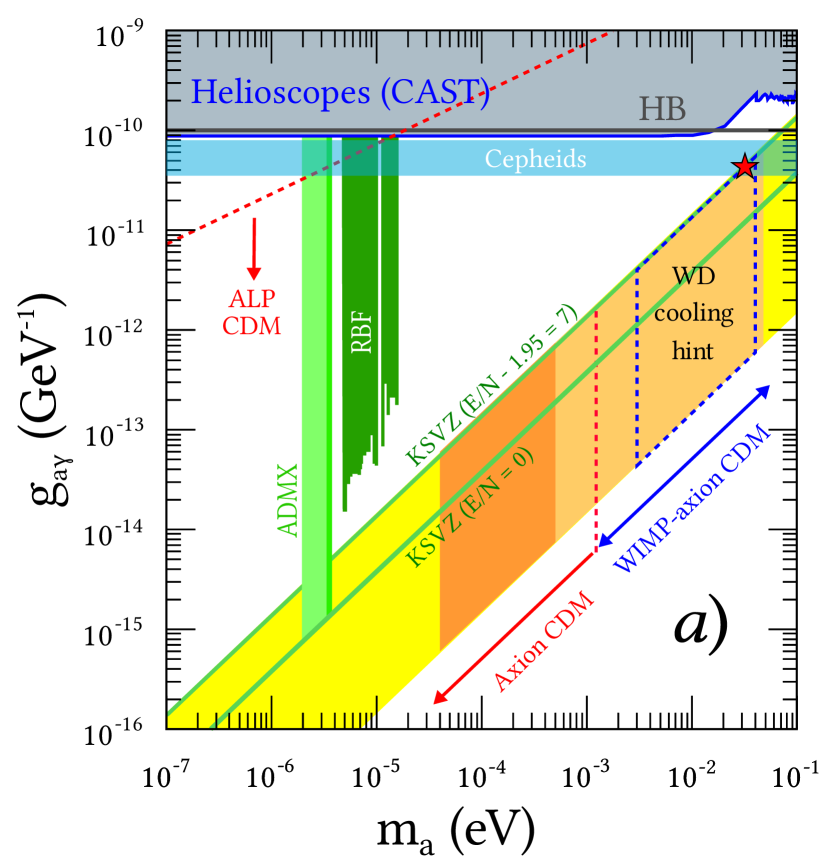
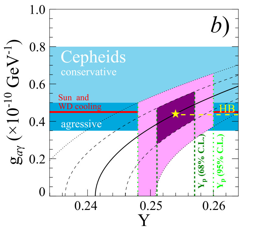
Figure 1: (a) Summary of astrophysical, cosmological and laboratory constraints on axions and ALPs. Comprehensive axion/ALP parameter space, highlighting two main front lines of direct detection experiments: helioscopes (CAST [13, 14, 15, 16]) and haloscopes (ADMX [17] and RBF [18]). The astrophysical bounds from horizontal branch and massive stars are labeled “HB” [2] and “Cepheids” [19], respectively. The QCD motivated models (KSVZ [20, 21] and DFSZ [22, 23]) for axions lay in the yellow diagonal band. The orange parts of the band correspond to cosmologically interesting axion models: models in the “classical axion window” possibly composing the totality of DM (labeled “Axion CDM”) or a fraction of it (“WIMP-axion CDM” [24]). For more generic ALPs, practically all allowed space up to the red dashed line may contain valid ALP CDM models [25]. The region of axion masses invoked in the white dwarf cooling anomaly is shown by the blue dashed line [26]. The red star marks the values of the axion mass $m_{a}\sim 3.2\cdot 10^{-2}eV$ and the axion-photon coupling constant $g_{a\gamma}\sim 4.4\cdot 10^{-11}GeV^{-1}$ chosen in the present paper on the basis of the suggested relation between the axion mechanisms of the Sun and the white dwarf luminosity variations.
(b) $R$ parameter constraints on $Y$ and $g_{a\gamma}$ (adopted from [27]). The dark purple area delimits the 68% C.L. for $Y$ and $R_{th}$ (see Eq. (1) in [27]). The resulting bound on the axion ($g_{10}=g_{a\gamma\gamma}/(10^{-10}~{}GeV^{-1})$) is somewhere between rather conservative $0.5<g_{10}\leqslant 0.8$ and most aggressive $0.35<g_{10}\leqslant 0.5$ [28]. The red line marks the value of the axion-photon coupling constant $g_{a\gamma}\sim 4.4\cdot 10^{-11}~{}GeV^{-1}$ chosen in the present paper. The blue shaded area represents the bounds from Cepheids observation. The yellow star corresponds to $Y$=0.254 and the bounds from HB lifetime (yellow dashed line).

It is very important that in our work the theoretical estimate for the fraction of the axion luminosity $L_{a}$ in the total luminosity of the Sun $L_{Sun}$ [13] with respect to (11) is

$$\frac{L_{a}}{L_{Sun}}=1.85\cdot 10^{-3}\left(\frac{g_{a\gamma}}{10^{-10}GeV^{-1}}\right)^{2}\sim 3.6\cdot 10^{-4}.$$ (13)

Thus, it is shown that the hypothesis about the possibility for the solar axions born in the core of the Sun to be efficiently converted back into $\gamma$-quanta in the magnetic field of the magnetic steps of the O-loop (above the solar overshoot tachocline) is relevant. The almost empty magnetic flux tubes with $B\sim 4.1\cdot 10^{7}~{}G$ (A) is the physical base for the almost zero gas pressure inside the tube, and consequently, the channeling of the photons of axion origin without absorption and scattering. As a result, the variations of the magnetic field in the solar tachocline are the direct cause of the converted $\gamma$-quanta intensity variations. The latter, in their turn, may be the cause of the overall solar luminosity variations known as the active and quiet Sun phases.

Considering the above remarks, we believe that it is necessary to calculate the effect of axion-originated photons in active and quiet phases of the Sun on the solar corona.

To do this, in Sec. 2 we first briefly examine the current problem of the corona heating.

In Sec. 2.1 we discuss the part of the axion and nanoflares spectra in the total solar spectrum during active and quiet phases of the Sun. In Sec. 2.2 we outline a scenario of corona heating by means of axion origin photons. In Sec. 2.3 we suggest a solution to the corona heating problem by means the photons of axion origin.

In Sec. 3 we obtain an indirect proof of the connection between the periods of S-stars near the black hole, and the sunspot cycles. Finally, in Sec. 4 we give a brief summary of this work.

2 Corona heating problem

An interesting problem arises here related to the heating of the practically empty magnetic tube (see Figs. 6a and 11 in [8]) and heating of the solar corona, which has long been unresolved (see [29, 30]). There are many assumptions about the unusually high temperature in the corona (see e.g. $T_{average}\approx(1.5-3)\cdot 10^{6}~{}K$ in [31] and [32, 33, 34, 35, 36, 37, 38]) compared to the chromosphere and photosphere. It is known that energy comes from the underlying layers, including, in particular, the photosphere and chromosphere. Here are just some of the elements, possibly involved in the heating of the corona: magneto-acoustic and Alfvén waves (see [39, 40, 41, 42, 43, 44, 45, 46, 47, 48, 49, 50, 51]), magnetic reconnections (see e.g. [52, 53, 54, 55, 56, 57]), nano-flares (see e.g. [58, 59, 60, 61, 62]), Ellerman bombs (see e.g. [53, 63, 64, 65]). It is considered (see e.g. [44]) that the possible mechanism of corona heating is the same as for the chromosphere: convective cells in the form of granulation rising from the depth of the Sun and appearing in the photosphere (see e.g. [46, 47, 66, 67]) lead to a local imbalance in the gas, which leads to the propagation of magneto-acoustic and Alfvén waves (see e.g. Fig. 13 in [36]) moving in different directions. In this case, a chaotic change in the density, temperature and velocity of the substance in which these waves propagate leads to a change in the speed, frequency and amplitude of the magneto-acoustic waves and can be so large that the gas becomes supersonic. Shock waves appear (see [68, 69, 70]), which lead to the heating of the gas and, as a consequence, to the heating of the corona.

On the other hand, we believe that the main effective mechanism for heating the solar corona is the emission of axions from the solar core with an energy spectrum with the maximum of about 3 keV and the average of 4.2 keV. These axions are supposed to convert into soft X-rays in very strong transverse magnetic field of an almost empty tube at the base of the convective zone (B). Eventually we suppose that the X-rays, through the axion-photon conversions in the magnetic O-loop near the tachocline, channel along the “cool” region of the Parker-Biermann magnetic tube (Fig. B.1) and effectively supply the necessary photons of axion origin “channeling” in an almost empty magnetic tube to the photosphere while the convective heat transfer is heavily suppressed (B). As a result, X-rays, passing through the photosphere at high speed and scattering in the Compton process, reach the transition region between the chromosphere and corona. The bulk of soft X-rays dissipates in the corona (see Fig. 3c,d).

The total power radiated by X-rays of axion origin is only about one millionth of the total solar luminosity, so there is sufficient energy on the Sun to heat the corona.

It should be recalled here that the energy distribution of the emitted axions is far from being a blackbody spectrum because the spectrum of the incident photons is modulated by the frequency dependence of the cross-section. For the typical solar spectrum, the maximum of the differential flux of axions occurs at $E_{a}/T\approx 3.5$, whereas the average axion energy is $\langle E_{a}/T\rangle\approx 4.4$ [7]. This means that the average energy of the photon of axion origin can generate a temperature of the order of $T_{a}\sim 1.11\cdot 10^{7}~{}K$ under certain conditions of coronal substances [71], which is close to the temperature $T_{core}\sim 1.55\cdot 10^{7}~{}K$ of the Sun core (see e.g. [72, 73, 74, 75]).

This raises an intriguing question about the paradoxical heating of the corona (see e.g. [76, 39, 77, 78, 79, 80, 81, 82, 83, 84, 85, 86, 87, 35, 88, 89, 90, 91, 92, 29, 62, 93, 49]): how do the soft X-rays of axion origin heat the solar corona and flares to a temperature of more than two and, correspondingly, three orders of magnitude higher than in the photosphere?

Below we show why the solar corona is so hot with the help of photons of axion origin.

2.1 The complete solar spectrum of nanoflares and axions in the solar atmosphere

From the axion mechanism point of view the solar spectra during the active and quiet phases (i.e. during the maximum and minimum solar activity) differ from each other by the soft part ($0.5~{}keV<E<2.0~{}keV$), where the power-law spectra of nanoflares prevail, or the hard part ($2~{}keV<E<10~{}keV$) of the Compton spectrum. The latter being produced by the photons of axion origin ejected from the magnetic tubes into the photosphere (see Fig. 2 and Fig. 4 in [94]).

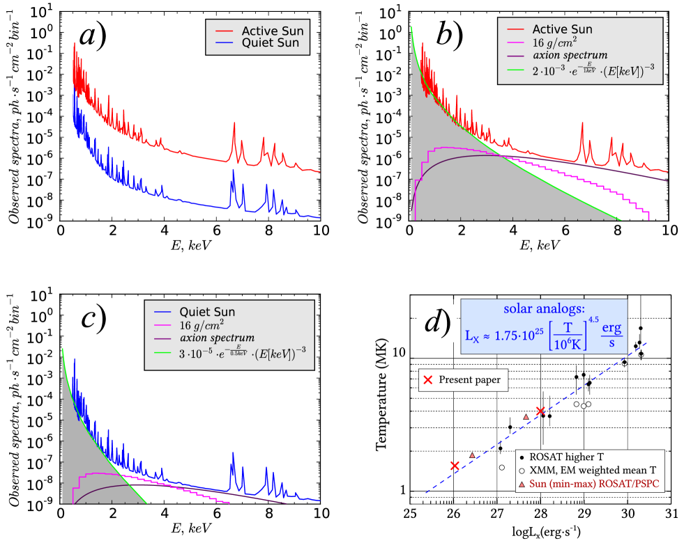
Figure 2: (a) Reconstructed solar photon spectrum in the 0.5 - 10 keV band from the active Sun (red line) and quiet Sun (blue line) from accumulated observations (spectral bin is 6.1 eV wide) [95].
(b) Reconstructed solar photon spectrum fit in the active phase of the Sun by the quasi-invariant soft part of the solar photon spectrum (grey shaded area; see Eq. (16)) and the spectrum (20) degraded to the Compton scattering for column density above the initial conversion place of 16 $g/cm^{2}$ (see Fig. 10 in [96]), and the initial energy distribution (thin line in violet) is the converted solar axion spectrum. Here the inverse Compton effect was not taken into account for the range 8 keV - 10 keV. Note that the GEANT4 code photon threshold is at 1 keV (reconstructed solar photon spectra from [95]).
(c) Similar curves for the quiet phase of the Sun (grey shaded area corresponds to Eq. (17)).
(d) Corona temperature against the X-ray luminosity of the solar analogs (see ROSAT, XMM-Newton, adopted from [97]). The data from ROSAT/PSPC are shown as compared to the maximum and minimum of the solar cycle (see Sect.3.3 in [95]).

A natural question arises at this point: “What are the real parts of the Compton spectrum of axion origin in the active and quiet phases of the Sun, and do they agree with the experiment?” Let us perform the mentioned estimations being based on the known experimental results by ROSAT/PSPC, where the Sun coronal X-ray spectra and the total luminosity during the minimum and maximum of the solar coronal activity were obtained [95].

Apparently, the solar photon spectrum below 10 keV of the active and quiet Sun (Fig. 2a) reconstructed from the accumulated ROSAT/PSPC observations can be described by two components: the first component is the soft ($0.5~{}keV<E<2.0~{}keV$) part of the spectrum where the power-law spectra of nanoflares dominate, and the second is the harder ($2~{}keV<E<10~{}keV$) part of the spectrum which was degraded to the Compton scattering for column density above the initial conversion place of 16 $g/cm^{2}$ (see Fig. 10 in [96]), and the initial energy distribution is the converted solar axion spectrum (Fig. 2b,c). The complete solar spectrum is:

$$\left(\frac{d\Phi}{dE}\right)^{(*)}\approx\left(\frac{d\Phi}{dE}\right)^{(*)}_{nanoflare}+\left(\frac{d\Phi_{\gamma}}{dE}\right)^{(*)}_{axions},$$ (14)

where ${d\Phi}/{dE}$ is the observed solar spectra during the active (red line in Fig. 2a,b) and quiet (blue line in Fig. 2a,c) phases, $\left({d\Phi}/{dE}\right)_{nanoflare}$ represents the power-law spectra of the nanoflares at 0.5-2.0 keV,

$$\left(\frac{d\Phi}{dE}\right)_{nanoflare}\sim E^{-(1+\alpha)}e^{-E/E_{0}},$$ (15)

where the power-law decay with the “semi-heavy tail” takes place in practice [98] instead of the so-called power laws with heavy tails [99, 98] (see e.g. Figs. 3 and 6 in [100]). Consequently, the observed corona spectra ($0.5~{}keV<E<2.0~{}keV$) (shaded area in Fig. 2b)

$$\left(\frac{d\Phi}{dE}\right)^{(active)}_{nanoflare}\sim 2\cdot 10^{-3}\cdot(E~{}[keV])^{-3}\cdot\exp{\left(-\frac{E}{1keV}\right)}$$

$$~{}~{}for~{}the~{}active~{}Sun$$ (16)

and (shaded area in Fig. 2c)

$$\left(\frac{d\Phi}{dE}\right)^{(quiet)}_{nanoflare}\sim 3\cdot 10^{-5}\cdot(E~{}[keV])^{-3}\cdot\exp{\left(-\frac{E}{0.5keV}\right)}$$

$$~{}~{}for~{}the~{}quiet~{}Sun;$$ (17)

$\left({d\Phi_{\gamma}}/{dE}\right)_{axions}$ is the reconstructed solar photon spectrum fit ($2~{}keV<E<10~{}keV$) built up from two spectra (see Fig. 2b,c for the active and quiet phases of the Sun, respectively).

As is known, this class of flare models (Eqs. (16) and (17)) is based on the recent paradigm in statistical physics known as self-organized criticality [101, 102, 103, 104, 105]. The basic idea is that the flares are a result of an “avalanche” of small-scale magnetic reconnection events cascading [98, 106, 107] through the highly intense coronal magnetic structure [108] driven at the critical state by the accidental photospheric movements of its magnetic footprints. Such models thus provide the natural and computationally convenient basis for the study of Parker’s hypothesis of the coronal heating by nanoflares [80].

Another significant fact discriminating the theory from practice, or rather giving a true understanding of the measurements against some theory, should be recalled here (see e.g. Eq. (15); also see Eq. (5) in [98]). The nature of power laws is related to the strong connection between the consequent events (this applies also to the “catastrophes”, which in turn give rise to a spatial nonlocality related to the appropriate structure of the medium (see page 45 in [100])). As a result, the “chain reaction”, i.e. the avalanche-like growth of perturbation with more and more resource involved, leads to the heavy-tailed distributions. On the other hand, obviously, none of the natural events may be characterized by the infinite values of the mean and variance. Therefore, the power laws like (15) are approximate and must not hold for the very large arguments. It means that the power-law decay of the probability density rather corresponds to the average asymptotics, and the “semi-heavy tails” must be observed in practice instead.

It is known [71] that traditionally in the atmosphere of the Sun there are three types of eruptions, such as coronal mass ejections, prominence eruptions and eruptive flares, and they are considered bound and are the result of the same physical process. Coronal mass ejections (CMEs) are large-scale mass ejections and magnetic flux from the lower corona to the interplanetary space. It is believed that they should be created by the loss of equilibrium in the structures of the coronal magnetic plasma, which causes sharp changes in the magnetic topology. A typical CME carries approximately $10^{23}~{}Mx$ of flux and $10^{13}~{}kg$ of plasma into space [71]. During the active phase of the solar cycle, CME can occur more often than once a day. The intermittent appearance of a new magnetic flux from the convective zone (which originates from twist in flux tubes (see [109, 110, 111]) in the corona is the most important process for the dynamic evolution of the coronal magnetic field [112, 113, 114, 115], in which the rearrangement of the intersection of closed coronal lines of force causes the accumulation of coronal field strength. When the stress exceeds a certain threshold, the stability of the magnetic field configuration is broken and erupts (see e.g. Fig. 3c; Fig. 2 in [56]). This model is called a storage model [116], although it is unfortunately known that the question of how magnetic fields rise from the tachocline to the convective zone of the Sun and exit through the photosphere and chromosphere into the corona has not yet been resolved (see e.g. [117, 118, 119]).

Figure 3: Top: Synthesized photon spectra of the corona and nanoflares. (a) The coronal total luminosity of the Sun (see Table 2 in [95]) in the ROSAT/PSPC band ranges from $\approx 2.7\cdot 10^{26}~{}erg/s$ at minimum to $\approx 4.7\cdot 10^{27}~{}erg/s$ at maximum. To calculate the observed spectra of the corona, we used abbreviated data ($0.5~{}keV<E<10.0~{}keV$) in [95] (Fig. 2a,b,c). (b) Simplified 2D schematic diagram of magnetic reconnection. Oppositely directed magnetic fields (light blue lines) and ambient plasma (light blue circles) move into the diffusion region (shaded box in the center), where magnetic reconnection occurs. The plasma is heated and accelerated into jets to the left and right (shaded blue ovals). Adopted from [120]. Bottom: The origin of magnetic flux and the associated dynamic coronal phenomenon on the Sun [56] and the appearance of the photon fluxes of axion origin. The blue and green dashed curves show the selected coronal loops representing the two lines of magnetic fields involved in the process (c) and (d). The sequence of extreme ultraviolet images clearly shows that two groups of oppositely directed and non-coplanar magnetic loops (c) gradually approach each other (d), causing a magnetic reconnection. If the plasma attracts magnetic loops, which gradually approach each other, causing magnetic reconnection, then nanoflares of two frequency types appear (see Fig. 4). In our case, when the plasma interacts with photons of axion origin, the magnetic reconnection of the nanoflare is the result of low-frequency heating. As a result, rather rare high-energy nanoflares occur with a low frequency, and the temperature rises sharply to about 10 MK. On the other hand, when the plasma exists without interacting with photons of axion origin, then frequent low-energy nanoflares occur, and the temperature fluctuations are insignificant (see Fig. 4).

Nevertheless, this plausible explanation is associated not only with the appearance of a magnetic flux, but also necessarily with the appearance of photons of axion origin from an empty magnetic tube (see Figs. 6a, 10a and 11 in [8]), in which, according to our theoretical and experimental observations (see Fig. 3a), the simultaneous occurrence of a magnetic flux and the flux of photons of axion origin in the outer layers of the Sun is the main mechanism of the formation of sunspots and active regions, being the integral part of the solar cycle, and also of the high energy release in the corona and flares. The physical solution of this problem will be shown below.

First about the flares. The well-known scenario of magnetic reconnection suggests that the corona is heated by numerous small-scale energy release events called nanoflares [80, 81, 62].

According to [62], “…’nanoflare’ is a term that is often used to describe an impulsive heating event. It was first coined by Parker [80], who envisioned a burst of magnetic reconnection. The meaning of nanoflare has since evolved. Here, as in our earlier work, we take it to mean an impulsive energy release on a small cross-field spatial scale without regard to physical mechanism. It is a very generic definition. Waves produce nanoflares (e.g. [81]). Much of the discussion in this paper concerns generic heating, including by waves, but some of it deals specifically with magnetic reconnection. The distinction should be obvious.”.

We are interested in heating with magnetic reconnection (see e.g. complementary figures Fig. 1 in [120] and Fig. 5 in [121]. Here, Figure 4 describes a unifying pattern that attempts to explain both the diffuse component of the corona and the clearly distinguishable coronal loops. Over most of the corona, low-energy nanoflares occur at a medium to high frequency, and temperature fluctuations are insignificant. Footpoint driving replenishes the magnetic energy extracted by each modest event in near real time, producing a statistical steady state. This is a diffuse corona: in the upper part, the delay between successive nanoflares is much less than the cooling time, so the temperature fluctuates around the average. This delay is called high frequency heating.

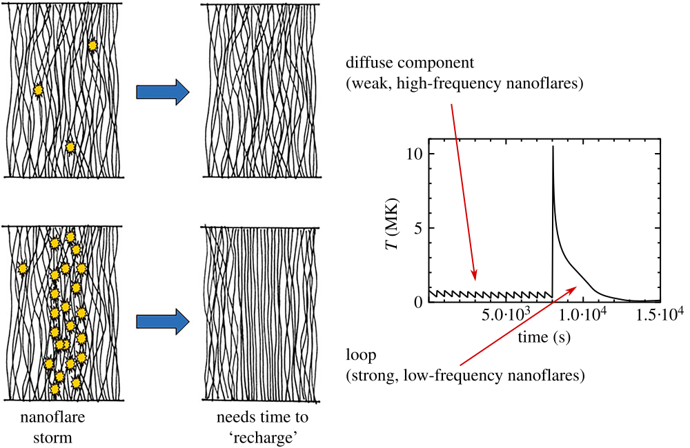
Figure 4: A unifying picture that explains both the diffuse component of the corona and distinct loops. Adapted from [62].

When a magnetic loop is formed in the diffuse corona, this means that the reconnection events increase sharply, forming high-energy nanoflares, while the temperature rises sharply. In this case, the delay between nanoflares is much longer than the cooling time, and the filament is completely cooled before reheating. It is the low-frequency heating that creates distinct loops.

Hence, the overall picture of magnetic reconnection is as follows. If the plasma attracts magnetic loops, which gradually come closer to each other, causing magnetic reconnection, then nanoflares appear with one of two types of event frequencies.

From here arises the question of what physics is behind the the two different event frequencies (see Fig. 4). In the first case, when the plasma interacts with photons of axion origin, magnetic reconnection of the nanoflare is the result of low-frequency heating. As a result, rather rare high-energy nanoflares occur with a low frequency, and the temperature rises sharply to about 10 MK. On the other hand, when the plasma (in magnetic reconnection) exists without the influence of photons of axion origin (see Fig. 4), there are frequent low-energy nanoflares, and the temperature fluctuations are insignificant.

Now let us get back to the second component in Eq. (14). The spectrum of solar photons below 10 keV for the active and quiet Sun (Fig. 2a), reconstructed from accumulated ROSAT/PSPC observations, can be described by the second (harder) component ($2~{}keV<E<10~{}keV$), which is degraded to Compton scattering for a column density above the initial conversion site of 16$g/cm^{2}$ (see Fig. 10 in [96]), while the initial energy distribution was the converted solar energy spectrum of axions (Fig. 2b,c).

In this regard we suppose that the application of the power-law distributions with semi-heavy tails leads to a soft attenuation of the observed corona spectra (which are not visible above $E>2~{}keV$), and thus to a close coincidence between the observed solar spectra and $\gamma$-spectra of axion origin (Fig. 2a,b,c), i.e.

$$\left(\frac{d\Phi}{dE}\right)^{(*)}\approx\left(\frac{d\Phi_{\gamma}}{dE}\right)^{(*)}_{axions}=\left(\frac{d\Phi_{\gamma}}{dE}\right)_{CAS}+\left(\frac{d\Phi_{\gamma}}{dE}\right)_{compton},$$ (18)

where the first component on the right is the converted solar axion spectrum (CAS), and the second one is the degraded spectrum due to multiple Compton scattering. The spectrum due to inverse Compton scattering (see Fig. 2b,c) is neglected here.

It means that the physics of the formation and ejection of the $\gamma$-quanta above $2~{}keV$ through the sunspots into corona is not related to the magnetic reconnection theory by e.g. [108], and on the one hand, it may produce the converted solar axion spectrum, i.e. the differential $\gamma$-spectrum of axion origin:

$$\left(\frac{d\Phi_{\gamma}}{dE}\right)_{CAS} =P_{a\rightarrow\gamma}\frac{d\Phi_{a}}{dE}~{}~{}cm^{-2}s^{-1}keV^{-1}\approx$$

$$\approx 6.1\cdot 10^{-3}P_{a\rightarrow\gamma}\frac{d\Phi_{a}}{dE}~{}ph\cdot cm^{-2}s^{-1}bin^{-1},$$ (19)

where the spectral bin width is 6.1 eV, $P_{a\rightarrow\gamma}$ is the probability describing the relative portion of photons of axion origin channeling along the magnetic tubes, according to [95],

$$\frac{d\Phi_{a}}{dE} =6.02\cdot 10^{10}\left(\frac{g_{a\gamma}}{10^{10}GeV^{-1}}\right)^{2}E^{2.481}\times$$

$$\times\exp\left(-\frac{E}{1.205}\right)~{}~{}cm^{-2}s^{-1}keV^{-1},$$ (20)

is the part of the differential solar axion flux at the Earth [13].

On the other hand, a single degraded spectrum due to multiple Compton scattering is also shown for the column density above the initial transformation point of $16~{}g/cm^{2}$, which actually agrees with the observed shape of the spectrum (see Fig. 2a,b,c).

This leads to one important assumption. Since the frequently occurring low-energy nanoflares are practically not associated with photons of axion origin (see Fig. 2b,c and Fig. 3c), we assume that the nanoflare temperature is of the order of $<10^{6}~{}K$ (see Fig. 4).

This means that, neglecting the effect of nanoflares, from the point of view of the axion mechanism, we should consider the spectra during active and quiet phases, in which the spectrum is dominated by photons of axion origin, ejected from magnetic tubes, from the photosphere to the corona (see Fig. 2a,b,c).

2.2 Scenario of coronal heating by means of axion origin photons

The main task here is to the study of the effect of virtually empty magnetic tubes in the convective zone and dark matter phenomena of solar axions.

Ultimately, the most important stages include not only the processes of magnetic energy release, in which magnetic energy is converted into heat, energetic particles and radiation, but also the plasma reaction to heating, in which it is organized using degraded spectra due to multiple Compton scattering closely related to the density columns above the initial conversion site (Fig. 2b,c), and the initial energy distribution, that is, the converted solar axion spectrum (Fig. 2b,c).

Let us remind here that in our view, the main effective mechanism for heating the solar corona is the emission of axions from the solar core with an energy spectrum with the maximum of about 3 keV and the average of 4.2 keV. These axions are supposed to convert into soft X-rays in very strong transverse magnetic field of an almost empty tube at the base of the convective zone (B). Eventually we suppose that the X-rays, through the axion-photon conversions in the magnetic O-loop near the tachocline, channel along the “cool” region of the Parker-Biermann magnetic tube (Fig. B.1) and effectively supply the necessary photons of axion origin “channeling” in an almost empty magnetic tube to the photosphere while the convective heat transfer is heavily suppressed (B).

The strong magnetic field (with $B\sim 10^{7}~{}G$) results not only in the strong suppression of convective heat transfer, but also in the conversion (in a magnetic O-shaped loop) of high-energy photons (from the radiation zone) into axions in the tachocline. The appearance of axions in the convective zone leads (then, and only then!) to the suppression of convective heat transfer. Thus the mean free path of a photon of axion origin in the convective zone is the result of the average length from the tachocline to the photosphere. The complete physics of this process is described in B.

Since we understand that a practically empty magnetic tube in the photosphere becomes a sunspot, then a question arises about the observational data from such magnetic tubes in the solar atmosphere (i.e. from the photosphere to the corona), from which photons are emitted. Curiously enough, the NuSTAR data highlighted in green (2 to 3 keV) and blue (3 to 5 keV) colors) reveal the high energy solar X-rays (see Fig. 5b), which clearly suggest the emission of photons of axion origin from the sunspots.

From here we understand that nanoflares and photons of axion origin in the corona can be born as nanoflares in penumbra (see Fig. 5c,d,e) and photons of axion origin in the umbra of the photosphere (see Fig. 5c).

We first “observe” photons of axion origin in the umbra of the photosphere (see Fig. 5c) based on images of the Sun at photon energies from 250 eV to several keV, obtained from the Japanese X-ray telescope Yohkoh (1991-2001) (see Fig. 5a), which show X-ray activity during the last minimum (in 1996) and maximum of the 11-year solar cycle. On the other hand, the first obtained image of the Sun by NASA’s Nuclear Spectroscopic Telescope Array (NuSTAR), made in high-energy X-rays, provides answers to questions about the extremely high temperatures observed over sunspots – cold dark spots in the Sun (see Fig. 5b).

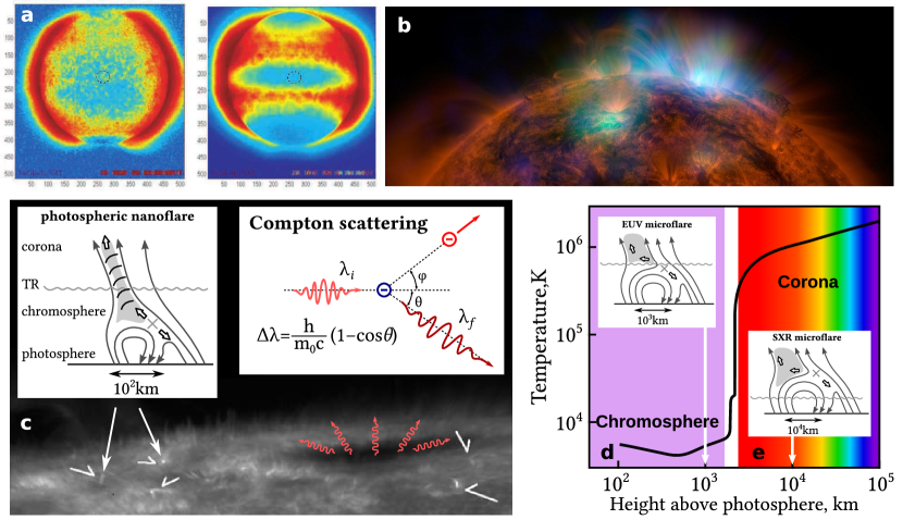
Figure 5: (a) Solar images at photon energies from 250 eV up to a few keV from the Japanese x-ray telescope Yohkoh (1991–2001) (see e.g. Fig.13 in [96]). On the left, a composite of 49 of the quietest solar periods during the solar minimum in 1996. On the right, solar X-ray activity during the following maximum of the 11-year solar cycle. (b) NuSTAR data, seen in green and blue, reveal solar high-energy emission (green shows energies between 2 and 3 keV, and blue shows energies between 3 and 5 keV). The high-energy X-rays come from gas heated to above 3 million degrees. The red channel represents UV light captured by SDO at wavelengths of 171Å, and shows the presence of lower-temperature material in the solar atmosphere at 1 million degrees (NASA/JPL-Caltech/GSFC, 2014). (c) Ca II H broadband filter snapshot image of the active region on 17 December 2006 near the west limb, taken with Hinode/SOT. The dark elongated ellipse seen near the limb is a sunspot (with umbra and penumbra). Numerous tiny jets ejected from bright points (arrows) can be seen. The footpoints of these jets are not a simple bright point, but show a cusp- or inverted Y-shape. This is the characteristic shape of X-ray jets, known as anemone jets (derived from Fig. 1 in [122]). Schematic illustration of axion origin photons flux from the umbra of sunspot (adapted from Fig. 1 in [122]), and the Compton scattering formula explaining the formation of a high electron temperature in the corona. (d),(e) Atmospheric temperature distribution near the solar surface (derived from Fig. 12 in [96]). Insets in (c),(d),(e) with transition regions (TR) illustrate the magnetic reconnections that occur at different altitudes, from the heights of the photosphere (c), continuing the chromosphere (d), and ending with the corona (e) (derived from Fig. 3 in [122]).

When an almost empty magnetic tube rises to the photosphere, the photons of axion origin, passing the upper boundary of the photosphere, are weakly scattered in the chromosphere, and then, passing the chromosphere, they are strongly scattered in the corona (Fig. 5d,e).

Recall that the essence of Compton scattering is the interaction of photons of axion origin with electrons of the outer layers of the Sun. Subsequently, this leads to an increase in the electron temperature and, as a consequence, to the heating of the plasma, the temperature of which is spatially equalized in the corona, and not only in the coronal loops. Moreover, in contrast to the local dissipation of nanoflares (Fig. 5c), the photons of axion origin, the “observed” energies of which are associated with red (0.3-1.0 keV), green (1.0-3.0 keV) and blue (3.0-10 keV) colors from inner spots (Fig. 5b), have a global space-time distribution (0.3-1.0 keV from Fig. 5b). This is directly related to the heating rate by photons of axion origin. In this case, the corona corresponds to an average temperature of about 1 MK with a red (0.3-1.0 keV) color (Fig. 5b). The nonlocal distribution of “observed” energies with green (1.0-3.0 keV) and blue (3.0-10 keV) colors (Fig. 5b) corresponds to the temperature above 3 MK. The global distribution does not contradict the fact that the corona is still hot, like 1 MK, even if there are no spots at some places (Fig. 5b).

Next, we are interested in the energy of photons of axion origin in the chromosphere and corona. The simplified answer is as follows. We know that the density of electrons in the chromosphere is higher than in the corona. When electrons in the chromosphere interact with photons of axion origin, the inverse Compton scattering increases the energy of the photons (to the right of the average axion energy in Fig. 3a) and thus decreases the energy of the electrons. A decrease in the energy of electrons leads to a decrease in temperature, and therefore, in the speed of electrons in the chromosphere (Fig. 5d). Conversely, when coronal electrons interact with photons of axion origin, the degraded Compton scattering decreases the energy of photons (to the left of the average axion energy in Fig. 3a) and thus increases the energy of the electrons. Therefore, we understand that an increase in the energy of electrons leads to an increase in temperature and, consequently, the speed of electrons in the corona (Fig. 5e). As a result, the accelerated high-speed electrons and protons, and generally, the continuous plasma flow propagating almost radially from the Sun and filling the Solar system up to the heliocentric distances of $\sim~{}100~{}a.u.$ (solar wind) is formed through the gas-dynamic expansion of the corona to the interplanetary space. At high temperatures in the solar corona ($1.5-4\cdot 10^{6}~{}K$) the pressure of overlying layers cannot compensate the gas pressure of the corona matter, and the corona expands. In such case the runaway solar wind moves along the open lines of magnetic field passing through the so-called coronal hole. The coronal holes are the areas in solar corona which are much less dense and less hot than the most of the corona, and therefore they are very thin. This promotes the solar wind, since it is easier for the particles to break through the chromosphere.

Finally, in Section 2.3 we show that the number of sunspots is equivalent to the number of magnetic flux tubes, and thus correlates with the fluxes of axion-origin photons, which in their turn correlate with the corona heating.

2.3 Solving the problem of corona temperature

Below we show how the plasma reaction to heating is organized through the interactions of the photon flux of axion origin with electrons in the outer layers of the Sun, at which a temperature above $10^{6}~{}K$ appears in the corona (see Eqs. (27) - (28); Fig. 2b,c,d)!

We assume that the probability $P_{\gamma}$ which describes the relative fraction of photons of axion origin propagating along the magnetic tube, and consequently, describes the relative fraction of the spot area, can be determined e.g. using $(P_{\gamma})_{max}$ at the maximum solar luminosity:

$$(P_{\gamma})_{max}=\left(P_{a\rightarrow\gamma}\right)_{max}\cdot\dfrac{2\left\langle sunspot~{}area\right\rangle_{max}}{(4/3)\pi R_{Sun}^{2}}\sim 0.74\cdot 10^{-2},$$ (21)

and during the minimum of Sun luminosity as:

$$(P_{\gamma})_{min}=\left(P_{a\rightarrow\gamma}\right)_{min}\cdot\dfrac{2\left\langle sunspot~{}area\right\rangle_{min}}{(4/3)\pi R_{Sun}^{2}}\sim 8.6\cdot 10^{-4},$$ (22)

where $\langle sunspot~{}area\rangle_{max}\approx 7.5\cdot 10^{9}~{}km^{2}\approx 2470~{}ppm$, $\langle sunspot~{}area\rangle_{min}\approx 9.0\cdot 10^{8}~{}km^{2}\approx 300~{}ppm$ of visible hemisphere is the sunspot area (over the visible hemisphere [123, 124]) for the cycle 22 experimentally observed by the Japanese X-ray telescope Yohkoh (1991) (see [96]); $R_{Sun}=6.96\times 10^{5}~{}km$; $P_{a\rightarrow\gamma}\approx 1$ at maximum of solar luminosity, and $P_{a\rightarrow\gamma}\approx 0.95$ at minimum (see Eqs. (119) and (120) in [8]).

The product of the total fraction of axions originating from the Sun core and the fraction of the sunspot area (see [123, 124]) yields the total fraction of the corona luminosity, or more precisely, the fraction of photon luminosity of axion origin in the corona.

$$\frac{L_{corona}^{X}}{L_{Sun}}=\frac{L_{a}^{*}}{L_{Sun}}\cdot P_{\gamma},$$ (23)

where $L_{corona}^{X}/L_{Sun}$ is the fraction of the corona luminosity in the total Sun luminosity, $L_{a}^{*}/L_{Sun}$ is the fraction of the axion “luminosity”, $L_{Sun}=3.8418\cdot 10^{33}~{}erg/s$ is the solar luminosity [125].

The axions luminosity fraction $L_{a}^{*}$ at the maximum and minimum of the Sun luminosity

$$\frac{(L_{a}^{*})_{max}}{L_{Sun}}=\frac{L_{a}-(L_{ADM})_{-}}{L_{Sun}}\sim 3.3\cdot 10^{-4},$$ (24)

$$\frac{(L_{a}^{*})_{min}}{L_{Sun}}=\frac{L_{a}-(L_{ADM})_{+}}{L_{Sun}}\sim 3.6\cdot 10^{-5},$$ (25)

are determined by the anticorrelated 11-year ADM density variations (with $(L_{ADM})_{+}/L_{Sun}\sim 3.24\cdot 10^{-4}$ and $(L_{ADM})_{-}/L_{Sun}\sim 3.24\cdot 10^{-5}$), which are gravitationally captured in the solar interior (see Sect. 3). Asymmetric dark matter provides a natural explanation of the comparable densities of baryonic matter and dark matter. The contribution of dark matter to the total mass of the star is totally negligible, but the presence of dark matter in the stellar interior changes the local properties of the plasma, and by doing so will affect the evolution of the star. We present models of dark matter with possible momentum- or velocity-dependent interactions with nuclei, based on direct detection and solar physics. An important note is that this, as a rule, can lead to the absence of self-annihilation today, which allows large amounts of ADM to accumulate in stars like the Sun [132]. Once the direct detection limits are accounted for, however, the best solution is spin-dependent $v^{2}$ scattering with a reference cross-section of $10^{-35}~{}cm^{2}$ (at a reference velocity of $v_{0}=220~{}km/s$, and a dark matter mass of about 5 GeV) (see [133]).

The ADM particles absorb energy in the hottest, central part of the core, they then travel to a cooler, more peripheral, area before the scattering again and redistribute their energy [134]. This reduces the contrast of temperature across the core region and reduces the central temperature. A colder core produces less neutrinos from the temperature-sensitive fusion reactions, and also less axions from the temperature-sensitive reactions of electron-nucleus collisions (see e.g. [7]). So the fluxes of ${}^{7}Be$ and ${}^{8}B$ neutrino, and axions (see (25)) can be significantly reduced. This is accompanied by a slight change in the $pp$ and $pep$ fluxes, as required by the constancy of the solar luminosity.

Taking into account the known observed variability of the corona luminosity in the X-ray range recorded in the ROSAT/SPC experiments,

$$\frac{(L_{corona}^{X})_{max}}{L_{Sun}}\sim 1.2\cdot 10^{-6},~{}~{}~{}\frac{(L_{corona}^{X})_{min}}{L_{Sun}}\sim 7.0\cdot 10^{-8},$$ (26)

we can compare the “experimental” (on the left; also (26)) and theoretical equations (on the right; also Eqs. (21) - (22) and (24)-(25))

$$\frac{(L_{corona}^{X})_{max}}{L_{Sun}}=\frac{(L_{a}^{*})_{max}}{L_{Sun}}\times(P_{\gamma})_{max}\sim 2.4\cdot 10^{-6},$$ (27)

$$\frac{(L_{corona}^{X})_{min}}{L_{Sun}}=\frac{(L_{a}^{*})_{min}}{L_{Sun}}\times(P_{\gamma})_{min}\sim 3.1\cdot 10^{-8},$$ (28)

which are good enough, but our estimates of the theoretical variations of solar luminosity $(L_{corona}^{X})_{max}\sim 1.0\cdot 10^{28}~{}erg/s$ at a temperature $T_{max}\sim 4\cdot 10^{6}~{}K$ and $(L_{corona}^{X})_{min}\sim 1.2\cdot 10^{26}~{}erg/s$ at a temperature $T_{min}\sim 1.5\cdot 10^{6}~{}K$ are still somewhat better than the data in [95] (see Fig. 2d).

At the same time, we must keep in mind that the “experimental” data (on the left: Eq. (26)) come from the spectra of the corona, synthesized with the MEKAL spectral code directly from the emission measure $EM(T)$ distribution derived with spectral fitting of ROSAT/PSPC spectra, as reported by [95] This means that the values of the “experimental” data (equation (26)) are rather rough due to their uncertainty, while the theoretical data (Eqs. (27)-(28)) are more accurate because of the temperature values (see Fig. 2d), which depend only on physics of the free energy accumulated by photons of axion origin in a magnetic field by means of degraded spectra due to multiple Compton scattering (see Fig. 2b,c), and which is rapidly released and converted into heat and plasma motion with a temperature of $\sim 4\cdot 10^{6}~{}K$ at maximum and $\sim 1.5\cdot 10^{6}~{}K$ at minimum of solar luminosity (see Fig. 2d).

From here we understand that the end result of the processes of the coronal magnetic energy release, which is converted into heat, energetic particles and radiation, would be described by a temperature of less than $10^{6}~{}K$ (see Eqs. (16)-(17); Fig. 2b,c). Meanwhile the reaction of the plasma to heating, in which it is realized by the interactions of the flux of the axion-originated photons with electrons in outer layers of the Sun, would be described by a temperature above $10^{6}~{}K$ (see Eqs.(27)-(28); Fig. 2b,c,d)!

Let us note another interesting point. In contrast to the variability of corona luminosity (on the left Eqs. (29) and (30)), according to the “experimental” ASCA/SIS data,

$$\frac{(L_{corona}^{X})_{max}}{L_{Sun}}\sim 0.39\cdot 10^{-6}\neq\frac{(L_{a}^{*})_{max}}{L_{Sun}}\cdot(P_{\gamma})_{max}\sim 2.4\cdot 10^{-6},$$ (29)

$$\frac{(L_{corona}^{X})_{min}}{L_{Sun}}\sim 0.6\cdot 10^{-8}\neq\frac{(L_{a}^{*})_{min}}{L_{Sun}}\cdot(P_{\gamma})_{min}\sim 3.1\cdot 10^{-8},$$ (30)

the strongest results is the theoretical variability of corona luminosity (on the right: Eqs. (29)-(30)), which coincide with the variations of the corona luminosity according to ROSAT/PSPC quite well (on the left: Eqs. (27)-(28)).

The preliminary result is as follows. If the hadron axions, arising from the Sun core, are controlled by 11-year variations of ADM density, that is gravitationally captured in the Sun interior (see Sect. 3), then the hard part of the spectrum of solar photons has the axion origin, which is determined mainly by theoretical estimate as the product of the fraction of axions in the Sun core and the fraction of the sunspot area (see [123, 124]). The latter is the result of the Sun luminosity variations (see Eqs. (27)-(28)). This means that the Sun luminosity variations and other solar cycles are the result of 11-year ADM density variations, which are anticorrelated with the density of hadron axions in the core of the Sun.

So on the basis of photons of axion origin, we obtain two significant results. First, the solar luminosity of the corona is absolutely identical to the luminosity of the photosphere (which is confirmed by Eqs. (27)-(28)), since the number of photons of axion origin, which exit through the magnetic flux tubes of the photosphere, despite the change in their density, is almost equal to the number of photons in the low-density ambient plasma of the corona. As a result, the experimental ratio $L_{corona}^{X}/L_{Sun}$ (see Fig. 3a) roughly coincides with the theoretical ratio $L_{a}^{*}/L_{Sun}\times P_{\gamma}$ (see e.g. Eqs. (27)-(28)) in the minimum and maximum luminosity of the corona.

Second, the energy distribution of the emitted axions is not like a blackbody spectrum, since the spectrum of the incident photons of axion origin is modulated by the frequency dependence of the cross section. As we have already shown, for a typical solar spectrum, the maximum of the axion differential flux occurs at $E_{a}/T\approx 3.5$, while the average axion energy $\langle E_{a}/T\rangle\approx 4.4$ [7]. This means that the energy of the average photon of axion origin can generate a temperature of the order of $T_{a}\sim 1.11\cdot 10^{7}~{}K$ (see e.g. Fig. 3a,c) under certain conditions of coronal substances, which is close to the temperature $T_{core}\sim 1.55\cdot 10^{7}~{}K$ of the solar core! As a result, the free energy accumulated by the photons of axion origin in a magnetic field by means of degraded spectra due to multiple Compton scattering (see Fig. 2b,c), is quickly released and converted into heat and plasma motion with a temperature of $\sim 4\cdot 10^{6}~{}K$ at maximum and $\sim 1.5\cdot 10^{6}~{}K$ at minimum of solar luminosity (see Fig. 2d). Under some conditions, the photons of axion origin with very powerful flares in the corona can partially generate energy, which corresponds to a temperature of the order of $T_{a}\sim 10~{}MK$ (see e.g. Fig. 3b,d).

As a result, according to our physical understanding, the coincidence of the theoretical (see e.g. Eqs. (27)-(28)) and experimental (see ROSAT/PSPC) photon spectra of the corona is connected, on the one hand, with the appearance of the magnetic flux and simultaneously the flux of photons of axion origin in the outer layers of the Sun, and on the other hand, with the manifestation of the basic mechanism of formation of sunspots and active regions correlated with the solar cycle, which determines the formation of the corresponding variation in the energy release of the axion-originated photons in the solar corona.

Curiously enough, we have understood that the fundamental physics of the Sun, as if recalling a forgotten, but physically profound question, raised long ago by R.H. Dicke, “Is there a chronometer hidden deep in the Sun?” [135, 136, 137], suggests the possibility of the existence of ADM (as a result of the energy conservation law with the Galactic frame velocity, density and dispersion) in the Sun core, with which, for example, variations in the ADM density and, as a consequence, variations in the neutrino flux, the solar cycle, solar luminosity, sunspots and other solar activities, seem to be paced by an accurate “clock” inside the Sun.

The question is very simple: If the ADM density variation controls the “clock” inside the Sun, then what is the physics behind this process?

3 How the ADM density variation around the black hole controls the ADM density variation inside the Sun

Let us try to find an answer to the important, yet unconventional question: is there an observable connection between the 11-year variations of ADM density in the solar interior and the periods of S-stars revolution around the SMBH at the center of the Milky Way (see e.g. [138, 139, 140])?

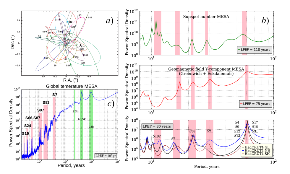
Figure 6: (a) Stellar orbits at the GC in the central arcsecond (declination Dec(”) as a function of time for the stars and red ascension R.A.(”)) [141, 138]. The coordinate system is chosen so that Sgr A* (the SMBH with the mass $\sim 4.3\cdot 10^{6}~{}M_{Sun}$ ) is at rest. (b) Power spectra of the sunspots (1874-2010 from Royal Greenwich Observatory), geomagnetic field Y-component (from Greenwich and Eskdalemuir observatories, [142]) and HadCRUT4 GST (1850-2012) (black), Northern Hemisphere (NH) and Southern Hemisphere (SN) using the maximum entropy spectral analysis (MESA); red boxes represent major astronomical oscillations associated to the major heliospheric harmonics associated to the orbits of the best known short-period S-stars (S0-102, S2, S38, S21, S4-S9-S12-S13-S17-S18-S31) at the GC [141, 138, 143, 144] and to the solar cycles (about 11-12, 15-16, 20-22, 29-30, 60-61 years). (c) Power spectra of the global temperature as reconstructed by [145]; red boxes represent the major astronomical oscillations associated to the major heliospheric harmonics associated to the orbits of the best known non-short-period S-stars (S19, S24, S66-S87, S97, S83, S?) at the GC [141, 138] and to the solar cycles (about 250, 330, 500, 1050, 1700, 3600 years); green boxes represent the major temperature oscillations presumably associated with the variations of the Earth orbital parameters: eccentricity ($\sim$93 kyr), obliquity ($\sim$41 kyr) and axis precession ($\sim$23 kyr).

On basis of the experimental data (see Fig. 6) on the oscillations of the sunspot number, the geomagnetic field Y-component and the global temperature we explicitly demonstrate that their periods coincide with revolution periods of S-stars orbiting a SMBH at the GC of the Milky Way. It is absolutely obvious that such a fine coincidence cannot be random. Then the next quite natural question arises: how do the solar and terrestrial observables “know” about motion of S-stars? And a hypothesis inevitably comes to mind: the “carrier” is none other than DM. More specifically, S-stars can modulate DM flows in our galaxy and, consequently, cause variations of DM space and velocity distributions, in particular, at the Sun and Earth positions. Further, these variations may cause the corresponding variations of the Solar System observables by means of some mechanism, e.g. the interaction of DM particles, which correlate with baryonic matter, with the cores of the Sun and the Earth. Such a probable mechanism is a subject of the current section. Here our aim is to stress that the available experimental data indicate the frequency transfer from the center of our galaxy to the Solar System. This fact can serve as an indirect evidence of the proposed hypothesis that DM plays the role of the variations carrier.

In order to answer this question, let us first consider all unexpected and intriguing implications of the 11-year modulations of ADM density in the solar interior and ADM around the BH.

The essence of fundamental magnetic processes associated with quantum gravity and the generalized thermomagnetic EN effect in the “tachocline” near the BH boundary may be described rather simply as follows. According to our understanding, one of the fundamental effects of the holographic principle of quantum gravity is the existence of “tachoclines” in all stellar objects in the Universe, including all galaxies and, of course, our Sun, magnetic white dwarfs, neutron stars and BHs of the Milky Way (see C).

Let us recall that the solar radiation zone rotates approximately like a solid, and the convection zone has a differential rotation. This leads to the formation of a very strong shear layer between these two zones, called the tachocline. Similar physics of the tachocline exists in a BH. As a result, the tachocline shear layers produce virtually empty MFTs (see B and Sect. 3.1.2 in [8]), anchored in the BH tachocline and rising to the surface of the disk (see Fig. 7b,d). Since it is known that disk parts rotate around a BH at different speeds that reinforce the fields (Fig. 7a), this turns the accretion disk into a vortex, pulling the substance into a BH and fueling winds that blow some of it outwards (see Fig. 7b).

So, if the physics of winds in the disk is identical to the physics of practically empty MFTs, which start from the tachocline and rise to the outer (Fig. 7c,d) or inner (Fig. 7a,b) part of the disk, then it means that the generalized thermomagnetic EN effect produces the magnetic tubes or the so-called winds and, on the one hand, the substance current flowing in the direction of the pole of the poloidal (meridional) field of the tachocline in the form of jets.

If we recall that the variations of the toroidal magnetic field and ADM density in the BH tachocline exactly anticorrelate with each other (see Eq. (33)), this means that in strong fields the magnetic tubes rise only inside the disk, which is equivalent to the disappearance of winds, and thus they slow down the speed of the accretion. And the opposite, in weak fields the magnetic tubes rise out of the disk surface (see Fig. 7c), which is equivalent to observing the disk winds, and thus they increase the speed of the accretion.

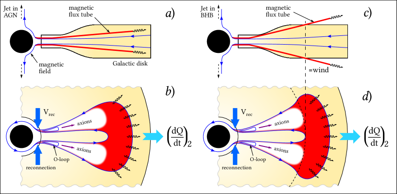
Figure 7: Schematic representation not to scale: Generalized thermomagnetic EN effect and virtually empty MFT born anchored to the BH tachocline and risen to the disk surface by the neutral buoyancy ($\rho_{ext}=\rho_{int}$; see also Figs. 9 and 11 in [8]). If the virtually empty magnetic flux tubes (B) are born with strong fields (a), then the flux tubes practically do not reach outside of the disk, while with less strong fields (c), the flux tubes go out of the disk at a small angle. So the visible (c,d) or invisible (a,b) buoyant flux tubes are the analog of the variation or disappearance of the wind through the various states of BH X-ray binaries (BHBs), which are interpreted as a variation in the driving mechanism of the wind (see [146] and Refs. therein). Based on the generalized thermomagnetic EN effect, the buoyancy of MFTs with the toroidal magnetic field $\gg 10^{5}~{}G$ in the BH tachocline, ultimately, through $\nabla\rho$-pumping (see Fig. 17,19 in [8]) with the magnetic field $\sim 10^{5}~{}G$ and the dominant Coriolis force creates an upward curved magnetic loop with a tilt angle from the Joy’s law (see (a), (c); see also Sect. 3.1.3.2 and Fig. 19a in [8]). The slope at low latitudes is near the disk plane (see (a), (c); see also Fig. 16a,b in [8]). Here the keV photons ((a)-(d); see analogous Fig. 11a in [8]), coming into the tachocline from the solar-like radiation zone, are turned (b,d) into axions by means of the horizontal magnetic field of the O-loop ((b,d); see analogous Figs. 6a, 9a and 11a in [8]). Some small photon flux can still pass through the “ring” between the O-loop and the tube walls (see Figs. 6a and 9a in [8]) and reach the solar-like penumbra of the MFT in the disk (see Fig. 9 and Sect. 3.1.3 in [8]). The physics and the possible estimate of the radiative heating $(dQ/dt)_{2}$ (see e.g. Fig. 11a in [8]; B) passing through the “ring” of the magnetic tube (b,d), the speed of the reconnection $V_{rec}$ (see analogous Fig. 12 in [8]; B), O-loops (see Figs. 6a, 9a, 10d, 11a in [8]), and the lifetime of the magnetic tube are presented in Sect. 3.1.3.1 in [8].

When the magnetic pressure is large at low densities and high temperatures, the low densities of the BH accretion material and high magnetic fields in the tachocline lead to the formation of highly collimated spectrally-hard jets, but without a “visible” magnetic tube (jet in AGN in Fig. 7c). And vice versa, when the magnetic pressure is relatively weak at high densities and low temperatures, the high density of the BH accretion material and relatively low magnetic fields in the tachocline lead to the formation of strongly collimated spectrally-soft jets and a visible magnetic tube, i.e. a visible disk “wind” (jet in BHB in Fig. 7c,d).

So, the resulting conclusion looks quite clear: the physical nature of the generalized thermomagnetic EN effect is the cause of both the formation of magnetic tubes rising from the BH tachocline to the disk and the formation of meridional currents in the direction of the BH pole, which generate jets, for example, in AGN or BHB.

Since the physics of magnetic tubes, rising from the BH “tachocline” to the disk, is almost identical, in our view, to the physics of visible or “invisible” disk winds, below we consider the common properties of the generalized thermomagnetic EN effect and the known models of disk winds. Curiously enough, the latter are associated with the mechanism of DM variations around a BH.

Such winds may arise from various processes, which makes their sources disputable (see e.g. [147] and Refs. therein). However, the X-ray spectroscopic data and analysis of the wind associated with the X-ray binary (XRB) GRO J1655-40 [148, 149, 150, 151, 152, 153] argued in favour of the magnetic origin, excluding all candidate processes except for the following two: the semi-analytic MHD wind model of [147] and the MHD outflow model of [146]. Plus our model of the generalized thermomagnetic EN effect.

The observations indicate that disk winds and jets in X-ray binaries are anticorrelated [149, 150, 151, 154, 155, 156, 157]. This indicates a link between disk properties, magnetic field configurations and outflow modes, the repulsive magnetic field induced by the generalized thermomagnetic EN effect (see Eq. (42), (48) in A), which produces the variations of the magnetic fields near the BH boundary (see e.g. [158, 159, 160]),

$$\frac{\left[B_{tacho}^{2}(r,t)\right]_{max-cycle}}{\left[B_{tacho}^{2}(r,t)\right]_{min-cycle}}=\frac{\left[n_{tacho}^{min}(r,t)\cdot T_{tacho}^{max}(r,t)\right]_{max-cycle}}{\left[n_{tacho}^{max}(r,t)\cdot T_{tacho}^{min}(r,t)\right]_{min-cycle}},~{}~{}~{}~{}~{}[T(r,t)]^{1/4}n(r,t)=const,$$ (31)

as well as the variations of the ADM density $n_{tacho}^{ADM}$ and baryon matter $n_{tacho}$,

$$\frac{\left[n_{tacho}^{min}(r,t)\right]_{max-cycle}}{\left[n_{tacho}^{max}(r,t)\right]_{min-cycle}}\approx\frac{\left[n_{tacho}^{ADM-min}(r,t)\right]_{max-cycle}}{\left[n_{tacho}^{ADM-max}(r,t)\right]_{min-cycle}}\,,$$ (32)

determined by the modulations of the ADM density $n_{tacho}^{ADM}$.

It is known (see [146]) that the X-ray spectra of BH X-ray binaries (BHBs) contain blueshifted absorption lines, which means the presence of outflowing winds. The observations also show that the disk winds are equatorial and they mostly occur in the Softer (disk dominated) states of the outburst, being less in the Harder (power-law dominated) states.

The properties of the accretion disk are used to infer the driving mechanism of the winds (see e.g. [161] and Refs. therein). And more or less prominent winds through the various states of the BHB have been interpreted as a variation in the magnetic driving mechanism of the wind [148, 149, 152, 161].

In our case the ADM density $n_{tacho}^{ADM}$ modulations, associated with the generalized thermomagnetic EN effect (see Eqs. (32), (33)), lead to the variations of the toroidal magnetic fields in the accretion disk (see Fig. 7). In order to understand the main motivation for the toroidal magnetic field variations in the accretion disk, forming the more or less significant winds, it is necessary to discuss the difference between the winds and jets from accretion disks.

Given Eq. (32) and the high (low) magnetic pressure, the density of ADM is relatively low (high), and the gas temperature is high (low). This means that with the high density of ADM and low temperature, the magnetic driving mechanism produces the accretion disk wind, which is equatorial (see 7b,d) and occurs in the soft states of the BHB outbursts (see e.g. the analogous model by [146]). Alternatively, with the low density of ADM and high temperature, the magnetic pressure is rather high and, consequently, the magnetic driving mechanism produces the weak or less prominent wind in the hard states (AGN jets).

Either way, the nonrelativistic disk winds and relativistic jets are anticorrelated, since the relativistic AGN jet, induced by the vertical toroidal magnetic field (see Fig. 7) and collisions between ADM and nuclei in the close vicinity of a SMBH (see e.g. the analogous model by [162]), is determined by the modulations of the ADM density (see Eq. (32)):

$$\frac{\left[B_{tacho}\right]_{max-cycle}}{\left[B_{tacho}\right]_{min-cycle}}=\left\{\frac{\left[\rho_{tacho}^{ADM-max}(r,t)\right]_{min-cycle}}{\left[\rho_{tacho}^{ADM-min}(r,t)\right]_{max-cycle}}\right\}^{3/2}.$$ (33)

This eventually means that the strong magnetic fields near the BH boundary are caused by quantum gravity of the dyonic BH [163], which determines the existence of the generalized thermomagnetic EN effect (A). So we understand that the major effect of quantum gravity here is that the initial acceleration (deceleration) of the disk winds and BHB flares (AGN jets) originate from less (more) strong magnetic fields in the accretion disk near the BH boundary (see also Eq. (33), Fig. 7), which predetermine the modulations of the ADM density – the process connected with the variability of the accretion flows, nonrelativistic disk winds and relativistic BHB or AGN jets.

This raises the question of how the observational data on AGN (or jet) variability, which theoretically anticorrelates with a variation of the toroidal magnetic field in the accretion disk, will be related to the observational data on variations in the accretion rate or e.g. the magnetic disk winds? In our opinion, despite the elusiveness of direct observations, some ideas, for example, of [164], about the possible observation of Parker loops from synchrotron radiation of galaxies near their edges, or from the Faraday rotation, or the idea of [146] on the possible observable difference between winds and jets from accretion disks can provide the indirect observational support.

In this sense, we are very interested in obtaining the indirect observations of anticorrelation between winds and jets from accretion disks. The point is that the modulation of a ADM halo leads to the situation when the high density of ADM corresponds to the disk wind and high accretion rate, while the low density of ADM corresponds to the low accretion rate and, as a result, to the jets from the BH. As we understand, in order to get a generalized picture of the connections between winds and jets from accretion disks, it is necessary to obtain the indirect observation, which physically explains the remarkable connection between all mentioned systems: the modulation of the ADM halo at the center of the galaxy $\rightarrow$ the vertical waves of density from the disk to the solar neighborhood [165, 166, 167, 168, 169, 170, 171, 172, 173, 174, 175] $\rightarrow$ variations (cycles) of sunspots $\rightarrow$ the variability of the local positions of orbital S-stars near the BH.

Our plan is the following. The main goal is to show that the observed variability of the local positions of the S-stars orbiting near the BH is an indicator (or dynamic probe) of the disk wind speeds variation or, equivalently, of the accretion rate variations of the BH. The intermediate goal is to briefly discuss the formation of the elliptically orbital distributions and periodic cycles of the S-stars, which are located in 0.13 ly $\approx$ 0.04 pc (see Fig. 26c in [8]) from the BH.

Here we present a detailed analysis of the effects of DM capture and energy transport on the structure and evolution of main-sequence B-stars, specifically those which might exist at the GC. First we need to highlight some important modulation properties of the S-stars and ADM around the BH:

$\bullet$ The greatest capture happens when the star is farthest from the center of the galaxy, at apoapsis. This is because it slows down relative to the ADM halo and achieves a significant capture rate for a time before turning back towards the BH. By the time it reaches periapsis, the star is moving so quickly that the capture is essentially zero, regardless of how high the ADM density is.

$\bullet$ When the S-stars, and especially, for example, S102 and S2, approach (retreat from) the center of the Milky-Way, at periapsis (apoapsis), the ADM density increases (decreases) and, thus, increases (decreases) the baryonic sector in the subparsec region near the SMBH at the GC. As a result, the variability of the ADM density and the baryonic matter density are determined by the variability of the gravitational potential around the BH, which is controlled by tidal interactions with other galaxies in the form of the Virgo-like cluster (see e.g. [176]).

We have found that, in contrast to the notable paper by [177], the presence of the intermediate mass BH (IMBH; see evidence by [178]) orbiting inside a nuclear star cluster at the GC can effectively help (by means of the AR-CHAIN code [179] and the “indirectly observable” ADM halo density modulation in the center of the Milky Way) to randomize the orbits of S-stars near the SMBH, converting the initially thin co-rotating disk (see the warped or mini-disk in Fig. 26c in [8]; see also [180, 181]) into the almost isotropic distribution of stars moving on eccentric orbits around the SMBH (see Fig. 8). Here the word “almost”, as we believe, practically overturns the essence of understanding of the physics of randomizing the orbits of S-stars near the SMBH, since the initial distribution of stars is somewhat ad hoc, and the evolution to the distribution of thermal eccentricity itself occurs at the even more special time scale.

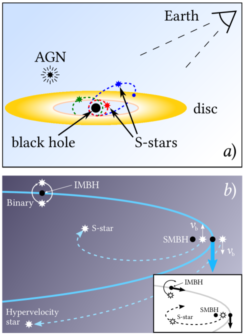
Figure 8: S-stars between the inner edge of the disk and the BH “tachocline”. (a) Simplified sketch of the observed variability of local positions of orbital S-stars near the BH. (b) Here is how the solution of the problem of energy conservation on the basis of four bodies works: a single body (SMBH) exchanges partners of binary stars orbiting around the IMBH, and through an extreme gravitational tidal field, one star is captured (by the SMBH) and loses energy, while the other runs away, gets all this energy and (through hypervelocity) just flies out of the galaxy (see [182, 183, 184, 185, 186, 187, 188, 189, 190, 191]). This is the so-called double slingshot. Inset: If two objects – an IMBH and a star rotating around it – are approaching a SMBH, then with three-body interactions the gravitational tidal field can be so extreme that it can separate the star from the IMBH. The capture or ejection of the star depends on the direction of motion of this star relative to the pair of BHs (SMBH-IMBH). Most likely, the star is captured by the SMBH. The resulting torus-like configuration is determined by the Kozai-Lidova eccentric mechanism in binary SMBHs (see e.g. analogous works by [192, 193, 189, 191]).

First of all, the randomization of the orbital planes requires $\leqslant 20~{}Myr$ (see [194]) if the IMBH mass is $(3.2\pm 0.6)\times 10^{4}~{}M_{Sun}$ (see [178]) and if the orbital eccentricity is $\sim 0.7$ or greater. So, this means that in our view of the S-stars randomization, the final distribution of the main semiaxes of star orbits does not depend on the estimated size of the IMBH orbit (see [177]) or, for example, on the special orientation of the binary orbit (see [195]), but depends on the “indirectly observable” density of the DM halo at the center of the Milky Way. Its time scale modulation is determined by the time scale of the S-stars periods through the variability of the gravitational potential at the GC, which is controlled by means of the “observed” disk wind rates variations or, equivalently, the accretion rate variations of the BH.

Let us now return to the question posed above. If we take into account the evolution of the SMBH-IMBH binaries through the case of the ejection of high-velocity S-stars (Fig. 8a) and B-type hypervelocity stars (Fig. 8b), i.e. the so-called IMBH slingshot, then how is the time scale of the S-stars periods (through the variability of the gravitational potential at the center of the galaxy) driven and controlled by the “observable” variations of the disk wind speeds or, equivalently, the variations of the BH accretion rate?

It works as follows. Among the chaotically oriented orbits of S-stars, some of them which are oriented near the fundamental plane of the GC have a direction along the accretion to the SMBH. When an elliptically orbital star moves from the BH periapsis (at the high speed the capture of ADM is almost zero) to apoapsis (when the speed is lower, the capture of ADM is not too small), it means that the point of apoapsis is determined by the condition of hydrostatic balance, at which the deceleration of the S-star must be identical (in the absolute value) to the deceleration of the disk wind, or equivalently, the lower BH accretion rate. Conversely, the increase in the speed of an elliptical-orbit star from apoapsis to periapsis assumes the higher speed of the disk wind, or equivalently, the higher rate of the BH accretion. As a result, the periods of variability in the disk wind speed or accretion rate are an indicator of the ADM variability, and consequently, an indicator of the periods of S-stars, e.g. S102 and S2 with periods of about 11 and 16 years (see Fig. 6a,b).

It also means that among the isotropically distributed S-stars there are such stars that, although they have random orientations, do not have random velocities and periods moving along eccentric orbits near the fundamental plane of the GC (see Fig. 8a).

A unique forecast of our model is the fact that the periods, velocities and modulations of S-stars are a fundamental indicator of the modulation of the ADM halo density in the fundamental plane at the center of the Galaxy, which closely correlates with the density modulation of the baryon matter near the SMBH. If the modulations of the ADM halo at the GC lead to modulations of the ADM density on the surface of the Sun (through vertical density waves from the disk to the solar neighborhood), then there is an “experimental” anticorrelation identity of the ADM density modulation in the solar interior and the number of sunspots. Therefore, this is also true for the correlation identity of the periods of S-star cycles and the sunspot cycles (see “experimental” anticorrelated data in Fig. 6a,b).

4 Summary and Outlook

By means of photons of axion origin, we obtain three main remarkable results.

$\bullet$ First, the solar luminosity of the corona is practically identical to the luminosity of the photosphere (which is confirmed by Eqs. (27)-(28)), since the number of photons of axion origin, which exit through the magnetic flux tubes of the photosphere, despite the change in their density, is almost equal to the number of photons in the low-density ambient plasma of the corona. As a result, the experimental ratio $L_{corona}^{X}/L_{Sun}$ (see Fig. 3a) is the same as the theoretical ratio $L_{a}^{*}/L_{Sun}\times P_{\gamma}$ (see e.g. Eqs. (27)-(28)) in the minimum and maximum solar luminosity.

$\bullet$ Second, this means that the average energy ($\langle E_{a}\rangle\approx 4.2~{}keV$ [7]) of the photon of axion origin can generate a temperature of the order of $T_{a}\sim 1.11\cdot 10^{7}~{}K$ (see e.g. Fig. 3a,c) under certain conditions of coronal substances, which is close to the temperature $T_{core}\sim 1.55\cdot 10^{7}~{}K$ of the solar core! As a result, the free energy accumulated by the photons of axion origin in a magnetic field by means of degraded spectra due to multiple Compton scattering (see Fig. 2b,c), is quickly released and converted into heat and plasma motion with a temperature of $\sim 4\cdot 10^{6}~{}K$ at maximum and $\sim 1.5\cdot 10^{6}~{}K$ at minimum of solar luminosity. It should be remembered that under some conditions, photons of axion origin with very powerful flares in the corona can partially generate energy, which corresponds to a temperature of the order of $T_{a}\sim 10~{}MK$ (see e.g. Fig. 3b,d).

$\bullet$ Third, we are interested in the existence of a dark matter chronometer hidden deep in the core of the Sun. The main reason is not the solar dynamos, which do not exist due to the strong magnetic fields, but the gravitational capture of asymmetric dark matter in the interior of the Sun. It depends on the holographic Babcock-Leighton mechanism as a consequence of the fundamental holographic principle of quantum gravity in the Sun.

A unique result of our model is that the physics of ADM halo modulation in the GC, which correlates with the modulation of the baryonic matter density near the supermassive black hole, leads to the ADM halo density modulations on the surface of the Sun (through the vertical density waves from the disk to the solar neighborhood). That is the “experimental” anticorrelation relationship between the ADM density modulation in the interior of the Sun and the number of sunspots. So it is indirectly proved that the ADM halo modulation in the GC is an indicator of the periods of S-stars, e.g. S102 with period of about 11 years, which are directly related to the identical periods of S-star cycles and the sunspot cycles.

This means that the S-star periods (see Fig. 6), starting from S102 with a period of about 11 years, S2 with period of about 16 years, S38 with period of about 22 years, S21 with period of about 30 years, and up to S4, S9, S12, S13, S17, S18, S31 with periods of about 60 years, are the indicators of the anti-correlation of periods of ADM density modulation inside the Sun, which, on the other hand, control the luminosity cycles of the Sun or sunspots.

But the main question is that we know the periods of the ADM density modulation inside the Sun, but, unlike the assumed maximum ($(L_{ADM})_{-}=1.2~{}\cdot~{}10^{29}~{}erg/s$) and minimum ($(L_{ADM})_{+}=1.2~{}\cdot~{}10^{30}~{}erg/s$) of solar luminosity, today we do not know how to calculate the 11-year ADM density modulation inside the Sun, which controls the modulation of solar luminosity.

In order to understand the physics of the 11-year modulation of the solar luminosity, we need a real interpretation of the energy transfer in the solar interior during the scattering of dark matter. However, taking into account the limits of significant indirect signals for detecting the results of an asymmetric dark mother with long-range interactions, where the residual annihilation of DM is enhanced by the Sommerfeld effect (see e.g. [130]), it is necessary to obtain the best solution of spin-dependent scattering $v^{2}$ with a cross section of $\sigma_{0}~{}cm^{2}$ (at a speed of $v_{0}=220~{}km/s$) and dark matter with a mass of about 5 GeV. This is a nontrivial result, first noted in [129], which deserves further study.

Appendix A Thermomagnetic Ettingshausen-Nernst effect of toroidal magnetic field in the tachocline

It is known [196] that the temperature dependence of the rate of a thermonuclear reaction is proportional to $T^{4.5}$ in the $10^{7}~{}K$ region. This means that there is a clear boundary between the hot region, which covers thermonuclear reactions and, as a consequence, high-energy photons (gamma rays) from the core to the outer edge of the radiative zone, and a colder region in which the dominant transport process (high-energy photons) changes to convection. This boundary between the radiative zone and the convection zone is the so-called tachocline. Because of the great temperature gradient in the tachocline, the thermomagnetic EN effect [197, 198, 199, 200] produces strong electric currents screening the intense magnetic fields $\sim 5\cdot 10^{7}$ G of the solar core [201, 202].

The thermomagnetic current can be generated in the magnetized plasma under the quasi-steady magnetic field in the weak collision approximation (the collision frequency much less than the positive ion cyclotron frequency) [203, 204]. For the fully ionized plasma the EN effect yields the current density (see Eqs. (5-49) and (5-52) in [203, 204]):

$$\vec{j}_{\perp}=\frac{3kn_{e}c}{2B^{2}}\vec{B}\times\nabla T$$ (34)

where $n_{e}$ is the electron number density, $B$ is the magnetic field, $T$ is the absolute temperature, $k$ and $c$ stand for the Boltzmann constant and the speed of light, respectively. When $n_{e}=\left[Z/(Z+1)\right]n$, where $n=n_{e}+n_{i}$, and $n_{i}=n_{e}/Z$ is the ion number density for a $Z$-times ionized plasma,

$$\vec{j}_{\perp}=\frac{3knc}{2B^{2}}\frac{Z}{Z+1}\vec{B}\times\nabla T.$$ (35)

It exerts a force on plasma, with the force density $F$ given by

$$\vec{F}=\frac{1}{c}\vec{j}_{\perp}\times\vec{B}=\frac{3nk}{2B^{2}}\frac{Z}{Z+1}\left(\vec{B}\times\nabla T\right)\times\vec{B}\,,$$ (36)

or with $\nabla T$ perpendicular to $\vec{B}$

$$\vec{F}=\frac{3nk}{2}\frac{Z}{Z+1}\nabla T\,,$$ (37)

which leads to the magnetic equilibrium (see Eq. (4-1) in [203]):

$$\vec{F}=\frac{1}{c}\vec{j}_{\perp}\times\vec{B}=\nabla p$$ (38)

with $p=nkT$. By equating (37) and (38),

$$\frac{3nk}{2}\frac{Z}{Z+1}\nabla T=nk\nabla T+kT\nabla n$$ (39)

or

$$a\frac{\nabla T}{T}+\frac{\nabla n}{n}=0,~{}~{}~{}where~{}~{}a=\frac{2-Z}{2(Z+1)},$$ (40)

we obtain the condition

$$T^{a}n=const.$$ (41)

For the singly ionized plasma with $Z=1$,

$$T^{1/4}n=const.$$ (42)

For the doubly ionized plasma ($Z=2$) $n=const$. Finally, in the limit of large $Z$, $T^{-1/2}n=const$, and $n$ does not depend on $T$ strongly, as opposed to the case of the plasma at a constant pressure with $Tn=const$. Thus, the thermomagnetic currents can change the pressure distribution in the magnetized plasma considerably.

Choosing the Cartesian coordinate system with $z$ axis along $\nabla T$, $x$ axis along the magnetic field and $y$ axis along the current, and assuming the fully ionized hydrogen plasma with $Z=1$ in the tachocline, we obtain

$${j}_{\perp}={j}_{y}=-\frac{3nkc}{4B}\frac{dT}{dz}.$$ (43)

From Maxwell’s equation $4\pi\vec{j}_{\perp}/c=\nabla\times\vec{B}$, one has

$${j}_{y}=\frac{c}{4\pi}\frac{dB}{dz},$$ (44)

then by equating (43) and (44) we derive

$$2B\frac{dB}{dz}=-6\pi kn\frac{dT}{dz}.$$ (45)

From (42) one has

$$n=\frac{n_{tacho}T_{tacho}^{1/4}}{T^{1/4}},$$ (46)

where the values $n=n_{tacho}$ and $T=T_{tacho}$ correspond to the overshoot tachocline. Substituting (46) into (45), we find

$$d\left(B^{2}\right)=-\frac{6\pi kn_{tacho}T_{tacho}^{1/4}}{T^{1/4}}dT.$$ (47)

As a result of integrating in the limits $[B_{tacho},0]$ on the left and $[0,T_{tacho}]$ on the right,

$$\frac{B_{tacho}^{2}}{8\pi}=n_{tacho}kT_{tacho}\,,$$ (48)

expressing the fact that the magnetic field of the thermomagnetic current in the overshoot tachocline “neutralizes” the magnetic field of the solar interior completely, so that the projections of the magnetic field in the tachocline and in the core are equal but of opposite directions (see Fig. A.1).

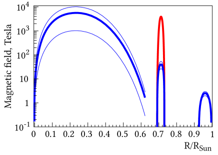
Figure A.1: The reconstructed solar magnetic field (in blue) simulation from [202]: 10³-10⁴ Tesla (left), 30-50 Tesla (middle) and 2-3 Tesla (right), with temperature of $\sim$9 MK, $\sim$2 MK and $\sim$200 kK, respectively. The thin lines show the estimated range of values for each magnetic field component. Internal rotation was not included in the calculation. An additional axion production can modify both intensity and shape of the solar axion spectrum (Courtesy Sylvaine Turck-Chièze (see Fig. 2 in [205])). The reconstructed solar magnetic field (in red) simulation from (50): $4\cdot 10^{3}$ T in tachocline ($\sim 0.7R_{Sun}$).

An intriguing question arises here of what forces are the cause of the shielding of the strong magnetic fields of the solar core and the radiation zone, which would be related to the enormous magnetic pressure in the overshoot tachocline,

$$\frac{B_{tacho}^{2}}{8\pi}=p_{ext}\approx 6.5\cdot 10^{13}\frac{erg}{cm^{3}}~{}~{}at~{}~{}0.7R_{Sun},$$ (49)

where the gas pressure $p_{ext}$ in the solar tachocline ($\rho\approx 0.2~{}g\cdot cm^{-3}$ and $T\approx 2.3\cdot 10^{6}K$ [74] at $0.7R_{Sun}$) yields the toroidal magnetic field

$$B_{tacho}\simeq 4100~{}T=4.1\cdot 10^{7}~{}G\,.$$ (50)

Propagating the question above even further, one may ask: “What kind of mysterious nature of the solar tachocline gives birth to the repulsive magnetic field through the thermomagnetic EN effect?” And finally, “If the thermomagnetic EN effect exists in the tachocline, what is its physical nature?” The essence of this physics will be discussed below.

Appendix B Almost empty magnetic flux tube nearby of the tachocline and physics of the mean free path of the axion-origin photon

It is known that the unsolved problem of energy transport by magnetic flux tubes at the same time represents another unsolved problem related to the sunspot darkness (see 2.2 in [206]). Of all the known concepts playing a noticeable role in understanding the connection between the energy transport and sunspot darkness, let us consider the most significant theory, in our view. It is based on the Parker-Biermann cooling effect [207, 208, 209] and originates from the early works of Biermann [208] and Alfvén [210].

As you know, the Parker-Biermann cooling effect [207, 208, 209], which plays a role in our current understanding, originates from Biermann [208] and Alfvén [210]: in a highly ionized plasma, the electrical conductivity can be so large that the magnetic fields are frozen into the plasma. Biermann realized that the magnetic field in the spots themselves can be the cause of their coolness – it is colder because the magnetic field suppresses the convective heat transfer. Hence, the darkness of the spot is due to a decrease in surface brightness.

Parker [207, 211, 212, 213, 209] has pointed out that the magnetic field can be compressed to the enormous intensity only by reducing the gas pressure within the flux tube relative to the pressure outside, so that the external pressure compresses the field. The only known mechanism for reducing the internal pressure sufficiently is a reduction of the internal temperature over several scale heights so that the gravitational field of the Sun pulls the gas down out of the tube (as described by the known barometric law $dp/dz=-\rho g$). Hence it appears that the intense magnetic field of the sunspot is a direct consequence of the observed reduced temperature [207].

On the other hand, Parker [213, 214] has also pointed out that the magnetic inhibition of convective heat transport beneath the sunspot, with the associated heat accumulation below, raises the temperature in the lower part of the field. The barometric equilibrium leads to enhanced gas pressure upward along the magnetic field, causing the field to disperse rather than intensify. Consequently, Parker [213] argued that the temperature of the gas must be influenced by something more than the inhibition of heat transport!

Currently it is believed (see [215]) that the ultimate goal is to simulate the formation of sunspots, where the convective heat transfer is either suppressed by a magnetic field [208] or the cooling is enhanced [211]. Thus, in general, it seems that we do not have a satisfactory explanation for the sunspot phenomenon yet. The question of the lack of energy flow or cooling, taking into account the magnetic field strength, remains open. According to [215], this will be another urgent goal for further research.

Our unique alternative idea is that the explanation of sunspots is based not only on the suppression of convective heat transfer by a strong magnetic field [208], but, in contrast to the enhanced cooling [211], the Parker-Biermann cooling effect appears as a result of the disappearance of barometric equilibrium [211], which is confirmed by axions of photonic origin from the photon-axion oscillations in the O-loop near the tachocline (see Fig. B.1).

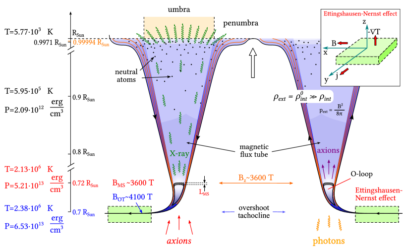
Figure B.1: Topological effects of magnetic reconnection inside the magnetic tubes with the “magnetic steps” (see Fig. 6 in Rusov et al. [8]). The left panel shows the temperature and pressure change along the radius of the Sun from the tachocline to the photosphere [74], $L_{MS}$ is the height of the magnetic shear steps. At $R\sim 0.72~{}R_{Sun}$ the vertical magnetic field reaches $B_{z}\sim 3600$ T, and the magnetic pressure $p_{ext}=B^{2}/8\pi\simeq 5.21\cdot 10^{13}~{}erg/cm^{3}$ [74]. Then a horizontal magnetic field is developed through the well-known Kolmogorov turbulent cascade (see Fig. B.2). The very cool regions along the entire convective zone caused by the Parker-Biermann cooling effect, have the virtually zero internal gas pressure because of the maximum magnetic pressure inside the magnetic tubes.

According to A, the $B\sim 4100$ T magnetic field in the overshoot tachocline and the Parker-Biermann cooling effect in an almost empty magnetic tube can produce the O-loops with the horizontal magnetic field $B_{MS}\approx B(0.72R_{Sun})\sim 3600$ T stretching for about $L_{MS}\sim 1.28\cdot 10^{4}~{}km$, (see e.g. Fig. 6ab in [8]), and surrounded by virtually zero internal gas pressure of the magnetic tube (see Fig. 6a in [8]). As an example, let us show Fig. B.1 and $p_{ext}=B_{0.72R_{Sun}}^{2}/8\pi=5.21\cdot 10^{13}~{}erg/cm^{3}$ [74].

On the other hand, we showed that the topological effects of magnetic reconnection inside magnetic tubes near the tachocline form the O-loop (Fig. B.2) through the Kolmogorov turbulent cascade (see Fig.13 in [8]). Their “magnetic steps” $L_{MS}$ participate in the formation of photons of axion origin (see Fig. B.1).

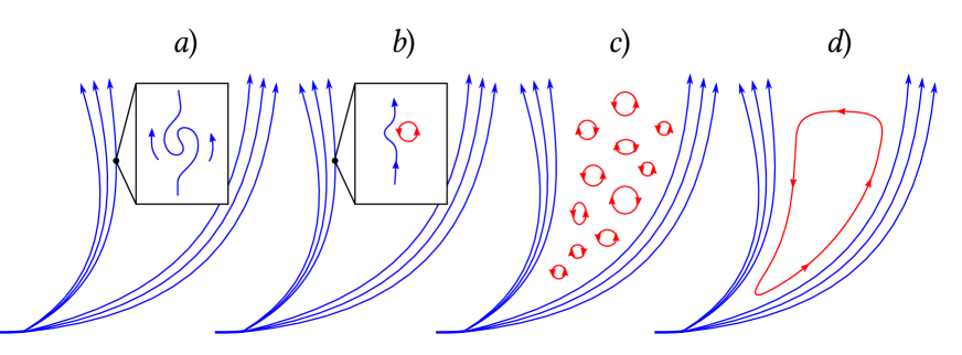
Figure B.2: Kolmogorov turbulent cascade [216, 217, 218] and magnetic reconnection in the lower layers inside a unipolar magnetic tube. Common to these various turbulent systems is the presence of the inertial range of Kolmogorov, through which the energy is cascaded from large to small scales, where dissipative mechanisms (as a consequence of magnetic reconnection) overcome the turbulent energy in plasma heating.

This rises another beautiful problem which is associated with our problem of almost total suppression of radiative heating in virtually empty magnetic tubes (see Fig. B.1). Let us remind that the high-energy photons going from the radiation zone through the horizontal field of the O-loop near the tachocline (Fig. B.1) are turned into axions, thus almost completely eliminating the radiative heating in the virtually empty magnetic tube. Some small photon flux can still pass through the “ring” between the O-loop and the tube walls and reach the penumbra (Fig. B.1).

Thus, the remarkable problem is that, on the one hand, there is a small flux of photons coming from the overshoot tachocline, which passes through the “ring” of a strong magnetic tube, which by means of convective heating physics $(dQ/dt)_{2}$ (see Fig. 7; Sect. 3.1.3.1 in [8]) allows one to determine both the lifetime of the magnetic flux tube from the tachocline to the surface of the Sun, and the reconnection rate $V_{rec}$, which is determined only by the process of magnetic loop raising and consequent sunspot vanishing from the surface of the Sun!

Therefore, as we understand, the existence of a magnetic O-loop (see Fig. B.2) and the Parker-Biermann cooling effect (Fig. B.1), which completely suppresses convection in an almost empty magnetic tube, is the cause of the sunspot darkness.

Finally, let us show the theoretical estimates of the Rosseland mean opacity and the axion-photon oscillations in the magnetic flux tubes.

It is essential to find the physical solution to the problem of solar convective zone which would fit the opacity experiments. The full calculation of solar opacities, which depend on the chemical composition, pressure and temperature of the gas, as well as the wavelength of the incident light, is a complex endeavor. The problem can be simplified by using the mean opacity averaged over all wavelengths, so that only the dependence on the gas physical properties remains (see e.g. [219, 220, 221]). The most commonly used is the Rosseland mean opacity $k_{R}$, defined as:

$$\frac{1}{k_{R}}=\left.\int\limits_{0}^{\infty}d\nu\frac{1}{k_{\nu}}\frac{dB_{\nu}}{dT}\middle/\int\limits_{0}^{\infty}d\nu\frac{dB_{\nu}}{dT}\right.\,,$$ (51)

where $dB_{\nu}/dT$ is the derivative of the Planck function with respect to temperature, $k_{\nu}$ is the monochromatic opacity at frequency $\nu$ of the incident light or the total extinction coefficient, including stimulated emission plus scattering. A large value of the opacity indicates strong absorption from beam of photons, whereas a small value indicates that the beam loses very little energy as it passes through the medium.

Note that the Rosseland opacity is the harmonic mean, in which the greatest contribution comes from the lowest values of opacity, weighted by a function that depends on the rate at which the blackbody spectrum varies with temperature (see Eq. (51) and Fig. B.3), and the photons are most efficiently transported through the “windows” where $k_{\nu}$ is the lowest (see Fig. 2 in [221]).

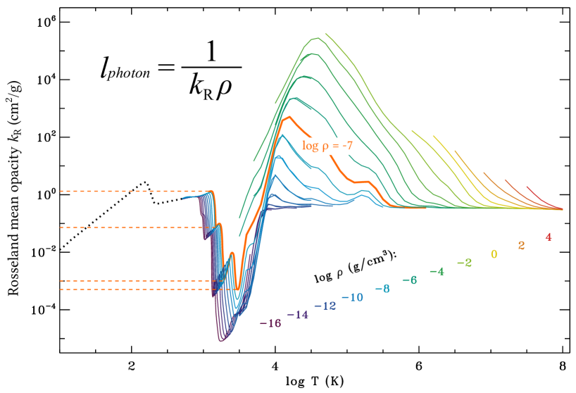
Figure B.3: Rosseland mean opacity $k_{R}$, in units of $cm^{2}g^{-1}$, shown versus temperature (X-axis) and density (multi-color curves, plotted once per decade), computed with the solar metallicity of hydrogen and helium mixture X=0.7 and Z=0.02. The panel shows curves of $k_{R}$ versus temperature for several “steady” values of density, labeled by the value of $\log{\rho}$ (in $g/cm^{3}$). Curves that extend from $\log{T}=3.5$ to 8 are from the Opacity Project (opacities.osc.edu). Overlapping curves from $\log{T}=2.7$ to 4.5 are from [220]. The lowest-temperature region (black dotted curve) shows an estimate of ice-grain and metal-grain opacity from [222]. Adopted from [67].

Taking the Rosseland mean opacities shown in Fig. B.3, one may calculate, for example, four consecutive cool ranges within the convective zone (Fig. B.1), where the internal gas pressure $p_{int}$ is defined by the following values:

$$p_{int}=nkT,~{}where~{}\begin{cases}T\simeq 10^{3.48}~{}K,\\ T\simeq 10^{3.29}~{}K,\\ T\simeq 10^{3.20}~{}K,\\ T\simeq 10^{3.11}~{}K,\\ \end{cases}\rho=10^{-7}~{}g/cm^{3}\,.$$ (52)

Since the inner gas pressure (52) decreases towards the surface of the Sun, so that

$$p_{int} (T=10^{3.48}~{}K)|_{\leqslant 0.85R_{Sun}}>p_{int}(T=10^{3.29}~{}K)|_{\leqslant 0.9971R_{Sun}}>$$

$$>p_{int}(T=10^{3.20}~{}K)|_{\leqslant 0.99994R_{Sun}}>p_{int}(T=10^{3.11}~{}K)|_{\leqslant R_{Sun}},$$ (53)

it becomes evident that the neutral atoms appearing in the upper convection zone ($\geqslant 0.85R_{Sun}$) cannot descend deep to the base of the convection zone, i.e. the tachocline (see Fig. B.1).

Therefore, it is very important to examine the connection between the Rosseland mean opacity and axion-photon oscillations in a magnetic flux tube.

In this regard let us consider the superintense magnetic $\Omega$-loop formation in the overshoot tachocline through the local shear caused by the high local concentration of azimuthal magnetic flux. The buoyant force acting on the $\Omega$-loop decreases slowly with concentration, so the vertical magnetic field of the $\Omega$-loop reaches $B_{z}\sim 3600$ T at about $R/R_{Sun}\sim 0.72$ (see Fig. B.1 and Fig. B.4b). Because of the magnetic pressure (see Fig. B.1) $p_{ext}=B_{0.72R_{Sun}}^{2}/8\pi=5.21\cdot 10^{13}~{}erg/cm^{3}$ [74], this leads to significant cooling of the $\Omega$-loop tube (see Fig. B.1).

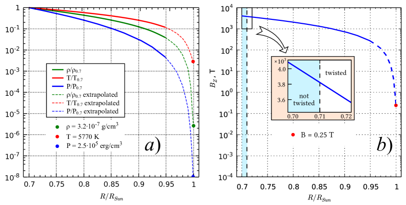
Figure B.4: (a) Normalized external temperature, density and gas pressure as functions of the solar depth $R/R_{Sun}$. The standard solar model with $He$ diffusion [74] was used for $R<0.95R_{Sun}$ (solid lines). The dotted lines mark extrapolated values. (b) Variation of the magnetic field strength $B_{z}$ along the emerging $\Omega$-loop as a function of the solar depth $R/R_{Sun}$ throughout the convection zone. The solid blue line marks the permitted values for the same standard solar model with $He$ diffusion [74] starting at the theoretical estimate of the magnetic field $B_{tacho}\approx 4100$ T. The dashed line is the continuation, according to the existence of the very cool regions inside the magnetic tube. The red point marks the up-to-date observations showing the mean magnetic field strength at the level $\sim 0.25~{}T=2500~{}G$ [223, 224].

Eventually we suppose that the X-rays, through the axion-photon oscillations in the magnetic O-loop near the tachocline, channel along the “cool” region of the Parker-Biermann magnetic tube (Fig. B.1) and effectively supply the necessary photons of axion origin “channeling” in the magnetic tube to the photosphere while the convective heat transfer is heavily suppressed.

In this context it is necessary to have a clear view of the energy transport by X-rays of axion origin, which are a primary transfer mechanism. The recent improvements in the calculation of the radiative properties of solar matter have helped to resolve several long-standing discrepancies between the observations and the predictions of theoretical models (see e.g. [219, 220, 221]), and now it is possible to calculate the photon mean free path (Rosseland length) for Fig. B.3:

$$l_{photon}=\frac{1}{k_{R}\rho}\sim\begin{cases}2\cdot 10^{10}~{}cm~{}~{}&for~{}~{}k_{R}\simeq 5\cdot 10^{-4}~{}cm^{2}/g,\\ 10^{10}~{}cm~{}~{}&for~{}~{}k_{R}\simeq 10^{-3}~{}cm^{2}/g,\\ 1.5\cdot 10^{8}~{}cm~{}~{}&for~{}~{}k_{R}\simeq 6.7\cdot 10^{-2}~{}cm^{2}/g,\\ 10^{7}~{}cm~{}~{}&for~{}~{}k_{R}\simeq 1~{}cm^{2}/g,\end{cases}~{}~{}\rho=10^{-7}~{}g/cm^{3}\,,$$ (54)

where the Rosseland mean opacity values $k_{R}$ and density $\rho$ are chosen so that the very low internal gas pressure $p_{int}$ (see Eq. (52)) along the entire magnetic tube almost does not affect the external gas pressure $p_{ext}$ (see (53) and Fig. B.3).

Let us now examine the appearance of the X-rays of axion origin, induced by the magnetic field variations near the tachocline (Fig. B.1), and their impact on the Rosseland length (see (53)) inside the cool region of the magnetic tubes.

Let us remind that the magnetic field strength $B_{tacho}\sim 4100$ T in the overshoot tachocline (see Fig. B.1) and the Parker-Biermann cooling effect (see Fig. B.1) lead to the corresponding value of the magnetic field strength $B(0.72R_{Sun})\sim 3600$ T (see Fig. B.1), which in its turn implies the virtually zero internal gas pressure of the magnetic tube.

As it is shown above, on the basis of Kolmogorov turbulent cascade (see Fig. B.2), the topological effect of the magnetic reconnection inside the $\Omega$-loop results in the formation of the so-called O-loops (Fig. B.1). It is possible to derive the value of the horizontal magnetic field of the magnetic steps at the top of the O-loop: $B_{MS}\approx B(0.72R_{Sun})\sim 3600$ T.

So in the case of the large enough Rosseland length (see Eq. (54)), X-rays of axion origin, induced by the horizontal magnetic field in O-loops, reach the photosphere freely, while in the photosphere itself, according to the Rosseland length

$$l_{photon}\approx 100~{}km<l\approx 300\div 400~{}km,$$ (55)

these photons undergo multiple Compton scattering producing a typical directional pattern (Fig. B.1).

Aside from the X-rays of axion origin with mean energy of $4.2~{}keV$ [13, 96], there are also $h\nu\sim 0.95~{}keV$ X-rays (originating from the interface between the radiation zone and overshoot tachocline, according to a theoretical estimate by [221]). Such X-rays would produce the Compton-scattered photons with mean energy of $\sim 0.95~{}keV$. These photons “disappear” by inverse X-ray transformation into axions (see Fig. B.1). This way the $\sim 0.95~{}keV$ X-rays do not contradict the known measurements of the photons with mean energy of $\sim 4~{}keV$ (see Fig. 1 in [13]) by involving the X-rays of axion origin in O-loops (see Figs. B.1).

And finally, let us emphasize that we have just shown a theoretical possibility of the time variation of the sunspot activity to correlate with the flux of the X-rays of axion origin; the latter being controlled by the magnetic field variations near the overshoot tachocline. As a result, it may be concluded that the axion mechanism for solar luminosity variations based on the lossless X-ray “channeling” along the magnetic tubes allows to explain the effect of the almost complete suppression of the convective heat transfer, and thus to understand the known puzzling darkness of the sunspots [206].

In addition to the energy source – photons of axion origin in the corona, which are the source of dark matter of axions in the core of the Sun, we are interested in the problems of both energy propagation and energy scattering.

This solution explicitly depends on the lifetime of the magnetic tubes rising from the tachocline to the solar surface. Therefore, because of the magnetic reconnection in the lower layers (see Fig. 4 in [225]), it is not the final stage of the simulation. The $\Omega$-loop, forming the sunspot umbra (Fig. B.5a) through the convection suppression from the tachocline to the photosphere, also gives rise to the convective upflow around the $\Omega$-loop forming the sunspot penumbra. Because of the pre-reconnection (Fig. B.5a,b) when the “legs” of the $\Omega$-loop collide (Fig. B.5b), the convective flow is generated at the base of the convection zone.

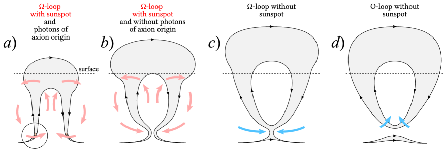
Figure B.5: A sketch of the magnetic reconnection near the tachocline. (a) $\Omega$-loop forms the sunspot umbra (with photons of axion origin) via the indirect thermomagnetic EN effect (A); (b) $\Omega$-loop with a sunspot (without photons of axion origin); pink arrows show the upward convective flow between the “legs” of the $\Omega$-loop during its rise from the tachocline to the visible surface; (c) $\Omega$-loop with reconnection and without a sunspot; (d) O-loop without a sunspot. Going through the stages (a), (b), (c), (d) (left to right), the convection around the rising $\Omega$-loop “closes” it at its base, then a free O-loop is formed via reconnection, and the initial configuration of the azimuthal field at the bottom of this region is restored. Blue arrows show the substance motion leading to the loop “legs” connection.

As we noted in Sec. 2.3, the intermittent appearance of a new magnetic flux from the convective zone (which originates from twist in flux tubes (see [109, 110, 111]) in the corona is the most important process for the dynamic evolution of the coronal magnetic field [112, 113, 114, 115], in which the rearrangement of the intersection of closed coronal lines of force causes the accumulation of coronal field strength. When the strength exceeds a certain threshold, the stability of the magnetic field configuration is broken and erupts in the form of nanoflares, the magnetic reconnection of which is associated with the escaping magnetic tube from the surface of the Sun, while the initial magnetic reconnection first occurs near the tachocline in the convective zone (see e.g. Fig. B.5c,d).

From here we understand that the flux of photons of axion origin, emitted from the photosphere of an almost empty magnetic tube (see Fig. B.5a), and the coronal magnetic field strength (which arises due to the twisting of the almost empty magnetic tubes, but without the sunspots (see Fig. B.5c,d)), have global and local space-time scales in the corona respectively.

This means that the photon flux of axion origin in the corona, which, on the basis of the plasma reaction to heating, is realized due to interaction with electrons in the outer layers of the Sun, has a global space-time scale and is a direct source of energy propagation, as well as the energy scattering!

Appendix C The fundamental holographic principle of tachocline

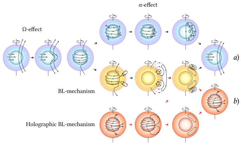
Figure C.1: An illustration of the main possible processes of a magnetically active star of the Sun type. (a) $\alpha$-effect, $\Omega$-effect and BL mechanism as components of the solar dynamo model. The $\Omega$-effect (blue) depicts the transformation of the primary poloidal field into a toroidal field by differential rotation. Regeneration of the poloidal field is then performed either by the $\alpha$-effect (top) or by the BL mechanism (yellow in the middle). In case of $\alpha$-effect, the toroidal field at the base of the convection zone is subject to cyclonic turbulence. In the BL mechanism, the main process of regeneration of the poloidal field (based on the $\Omega$-effect (blue)) is the formation of sunspots on the surface of the Sun from the rise of floating toroidal flux tubes from the base of the convection zone. The magnetic fields of these sunspots closest to the equator in each hemisphere diffuse and join, and the field due to the spots closer to the poles has a polarity opposite to the current that initiates rotation of the polarity. The newly formed polar magnetic flux is transported by the meridional flow to deeper layers of the convection zone, thereby creating a new large-scale poloidal field. Adapted from [226]. (b) BL mechanism and holographic BL mechanism as components of our solar antidynamo model. Unlike the component of the solar dynamo model (a), the BL mechanism, which is predetermined by the fundamental holographic principle of quantum gravity, and consequently, the formation of the thermomagnetic EN effect (see [203, 204, 227]), emphasizes that this process is associated with the continuous transformation of toroidal magnetic energy into poloidal magnetic energy ($T\rightarrow P$ transformation), but not vice versa ($P\rightarrow T$). This means that the holographic BL mechanism is the main process of regeneration of the primary toroidal field in the tachocline, and thus, the formation of floating toroidal magnetic flux tubes at the base of the convective zone, which then rise to the surface of the Sun. The joint connection between the poloidal and toroidal magnetic fields is the result of the formation of the so-called meridional magnetic field, which goes to the pole in the near-surface layer, and to the equator at the base of the convection zone.

The problem is devoted to the study of physics and the magnitude of the toroidal magnetic field in the tachocline. It is known that the radiation zone of the Sun rotates approximately as a solid body, and the convection zone has a differential rotation. This leads to the formation of a very strong shear layer between these two zones, which is called the tachocline. This gives rise to a fairly simple and at the same time very complicated question: “What is the nature and the consequence of the existence of tachoclines on the Sun or other stars?”

We propose a very unexpected answer that the existence of a two-dimensional surface of the tachocline in solar interior is the manifestation of the holographic principle in the Universe and, therefore, on the Sun. It is important to note that the holographic theory correlates the physical laws that act in some volume with the laws that act on the surface that limits this volume. The physics at the boundary is represented by quantum particles that have “colored” charges and interact almost like quarks and gluons in standard particle physics. The laws in the volume are a kind of string theory that includes the force of gravity (see [228]), which is difficult to describe in terms of quantum mechanics. The main result of the holographic principle is the fact that surface physics and physics in the volume are completely equivalent, in spite of the completely different ways of describing them.

In most situations, the contradictory requirements of quantum mechanics and general relativity are not a problem, because either quantum or gravitational effects are so small that they can be neglected. However, with a strong curvature of space-time, the quantum aspects of gravity become essential, and the conflict between the theory of gravity and quantum mechanics should disappear (see [229, 230, 231, 232]). To create a large curvature of space-time, a very large mass or density is required. Some physicists believe that even the Sun is incapable of distorting space-time so that the manifestations of quantum gravity effects become obvious.

Unlike other physicists, we believe that the fundamental holographic principle of quantum gravity predicts the experimental possibility of observational measurements of magnetic fields between the two-dimensional surface of the tachocline and the three-dimensional volume of the core on compact objects – our Sun, magnetic white dwarfs, accreting neutron stars and BHs.

This is due to the fact that in addition to the postulate of the Hooft’s brick wall [229], by now there is a lot of evidence that the physics of anti-de Sitter/conformal field theory correspondence (AdS/CFT) is correct. In addition, there are some derivations based on physical arguments.

Below we show the connection between the black hole in AdS/CFT and the tachocline of our Sun.

In theoretical physics the AdS/CFT correspondence ([233, 231]), sometimes referred to as “the Maldacena duality” or “the gauge/gravity duality” (see [234, 235, 236]), represents a hypothetical connection between two different types of physical theories – the gravitation theory and the quantum field theory. The AdS spaces used in the quantum gravitation theory formulated in terms of the string theory or M-theory [237] are on the one hand. The conformal field theories (CFTs), which are the quantum field theories including those similar to the Yang-Mills theories (see e.g. [238, 239]) describing the elementary particles, are on the other hand. Such equivalence is an example of the holographic duality – a representation of the 3D space on the 2D photographic emulsion (see [229, 230, 232]). Thus, although these two types of theories seem to be very different, they are mathematically identical [231, 234, 235]).

For example, according to [232], a remarkable property of the holographic principle of quantum gravity was obtained by Monte Carlo simulation of the dual gauge theory for the parameters corresponding to a black hole, which is destabilized due to the effects of quantum gravity. The major results of [232] for the black hole mass are exactly consistent with the prediction by [240] obtained from independent calculations in gravity theory at the leading order of quantum corrections. [232] thus obtained a quantitative evidence that the dual gauge theory proposed in superstring theory provides a correct description of a black hole, including the effects of quantum gravity.

Thus, we understand the connection between the black hole in AdS/CFT and the tachocline of our Sun.

It means that, using the thermomagnetic EN effect, a simple estimate of the magnetic pressure of an ideal gas in the tachocline of e.g. the Sun can indirectly prove that by using the holographic principle of quantum gravity, the repelling toroidal magnetic field of the tachocline exactly “neutralizes” the magnetic field in the Sun’s core

$$B_{tacho}^{Sun}=4.1\cdot 10^{7}~{}G=-B_{core}^{Sun}$$ (56)

(see Eq. (50) and Fig. A.1) where the projections of the magnetic fields of the tachocline and the core have the equal value but the opposite directions.

Such strong magnetic fields in a tachocline of e.g. the Earth, magnetic white dwarfs, accreting neutron stars and BHs can predict the exact “neutralization” of the magnetic field in the core of these stars and in a black hole (see Sect. 4 in [8]).

Let us note another important Babcock-Leighton (BL) mechanism (see Fig. C.1). On the one hand, we mark out the holographic BL mechanism (Fig. C.1b), which we often refer to as the holographic antidynamo mechanism, caused by a remarkable example of the Cowling antidynamo theorem. This theorem states that no axisymmetric magnetic field can be maintained through the self-sustaining action of the dynamo by means of an axially symmetric current [241]. On the other hand, the holographic BL mechanism (as a component of our solar anti-dynamo model) follows our example of a thermomagnetic EN effect, or the so-called solar holographic antidynamo, in which the poloidal field originates directly from the toroidal field, as shown in Fig. C.1b, but not vice versa (see Fig. C.1a).

References

- [1] G. G. Raffelt, Axions and other very light bosons: Part II (astrophysical constraints), Phys. Lett. 592 (2004) 391.
- [2] G. G. Raffelt, Astrophysical axion bounds, Lect. Notes Phys. 741 (2008) 51–71, arXiv:hep-ph/0611350.
- [3] M. Fairbairn, T. Rashba, S. Troitsky, Photon-axion mixing and ultra-high-energy cosmic rays from BL Lac type objects – shining light through the universe, Phys. Rev. D 84 (2011) 125019.
- [4] G. Raffelt, L. Stodolsky, Mixing of the photon with low-mass particles, Phys. Rev. D 37 (1988) 1237.
- [5] A. Mirizzi, G. G. Raffelt, P. D. Serpico, Photon axion conversion as a mechanism for supernova dimming: Limits from CMB spectral distortion, Phys. Rev. D 72 (2005) 023501.
- [6] K. Hochmuth, G. Sigl, Effects of axion-photon mixing on gamma-ray spectra from magnetized astrophysical sources, Phys.Rev. D 76 (2007) 123011.
- [7] G. G. Raffelt, Astrophysical axion bounds diminished by screening effects, Phys. Rev. D 33 (1986) 897–909. doi:10.1103/PhysRevD.33.897.
- [8] V. Rusov, M. Eingorn, I. Sharph, V. Smolyar, M. Beglaryan, Thermomagnetic ettingshausen-nernst effect in tachocline, magnetic reconnection phenomenon in lower layers, axion mechanism of solar luminosity variations, coronal heating problem solution and mechanism of dark matter spike variations around black hole, arXiv:1908.06042 [astro-ph.SR] (2019).
- [9] W. A. Bardeen, S.-H. Tye, Current algebra applied to properties of the light higgs boson, Physics Letters B 74 (3) (1978) 229–232. doi:10.1016/0370-2693(78)90560-9.
- [10] R. D. Peccei, H. R. Quinn, Cp conservation in the presence of pseudoparticles, Physical Review Letters 38 (25) (1977) 1440–1443. doi:10.1103/PhysRevLett.38.1440.
- [11] S. Weinberg, A new light boson?, Physical Review Letters 40 (4) (1978) 223–226. doi:10.1103/PhysRevLett.40.223.
- [12] F. Wilczek, Problem of strong and invariance in the presence of instantons, Phys. Rev. Lett. 40 (1978) 279–282. doi:10.1103/PhysRevLett.40.279.
- [13] S. Andriamonje, et al., An improved limit on the axion-photon coupling from the CAST experiment, J. Cosmol. Astropart. Phys. 10 (2007) 0702, arXiv:hep-ex/0702006.
- [14] Arik, E. et al. (CAST collaboration), Probing ev-scale axions with cast, Journal of Cosmology and Astroparticle Physics 2009 (02) (2009) 008.
- [15] Arik, E. et al. (CAST collaboration), Search for sub-ev mass solar axions by the cern axion solar telescope with buffer gas, Phys. Rev. Lett. 107 (2011) 261302. doi:10.1103/PhysRevLett.107.261302.
- [16] M. Arik, S. Aune, K. Barth, A. Belov, S. Borghi, et al., CAST solar axion search with 3He buffer gas: Closing the hot dark matter gap, arXiv:1307.1985 (2013).
- [17] S. J. Asztalos, G. Carosi, C. Hagmann, D. Kinion, , K. van Bibber, J. Hoskins, J. Hwang, P. Sikivie, D. B. Tanner, R. Bradley, J. Clarke, SQUID-based microwave cavity search for dark-matter axions, Phys. Rev. Lett. 104 (2010) 041301.
- [18] W. U. Wuensch, S. D. Panfilis-Wuensch, Y. K. Semertzidis, J. T. Rogers, A. C. Melissinos, H. J. Halama, B. E. Moskowitz, A. G. Prodell, W. B. Fowler, F. A. Nezrick, Results of a laboratory search for cosmic axions and other weakly coupled light particles, Phys. Rev. D 40 (10) (1989) 3153–3167.
- [19] G. Carosi, A. Friedland, M. Giannotti, M. Pivovarov, J. Ruz, J. Vogel, Probing the axion-photon coupling: phenomenological and experimental perspectives. a snowmass white paper, arXiv:1309.7035 (2013).
- [20] J. Kim, Weak interaction singlet and strong CP invariance, Phys. Rev. Lett. 43 (1979) 103.
- [21] M. Shifman, A. Vainshtein, V. Zakharov, Can confinement ensure natural CP invariance of strong interactions?, Nucl. Phys. B 166 (1980) 493.
- [22] A. P. Zhitnisky, On possible suppression of the axion hadron interactions (in Russian), Sov. J. Nucl. Phys. 31 (1980) 260.
- [23] M. Dine, W. Fischler, M. Srednicki, A simple solution to the strong {CP} problem with a harmless axion, Physics Letters B 104 (3) (1981) 199 – 202. doi:10.1016/0370-2693(81)90590-6.
- [24] H. Baer, A. Lessa, S. Rajagopalan, W. Sreethawong, Mixed axion/neutralino cold dark matter in supersymmetric models, JCAP 31 (2011).
- [25] P. Arias, D. Cadamuro, M. Goodsell, J. Jaeckel, J. Redondo, et al., WISPy cold dark matter, JCAP 13, arXiv:1201.5902 (2012).
- [26] I. G. Irastorza, The International Axion Observatory IAXO. Letter of Intent to the CERN SPS committee, Tech. Rep. CERN-SPSC-2013-022. SPSC-I-242, CERN, Geneva (Aug 2013).
- [27] A. Ayala, I. Domínguez, M. Giannotti, A. Mirizzi, O. Straniero, Revisiting the bound on axion-photon coupling from globular clusters, Phys. Rev. Lett. 113 (2014) 191302. doi:10.1103/PhysRevLett.113.191302.
- [28] A. Friedland, M. Giannotti, M. Wise, Constraining the axion-photon coupling with massive stars, Phys. Rev. Lett. 110 (2013) 061101. doi:10.1103/PhysRevLett.110.061101.
- [29] I. De Moortel, P. Browning, Recent advances in coronal heating, Philosophical transactions. Series A, Mathematical, physical, and engineering sciences 373 (2015) 2042. doi:10.1098/rsta.2014.0269.
- [30] I. D. Moortel, D. J. Pascoe, A. N. Wright, A. W. Hood, Transverse, propagating velocity perturbations in solar coronal loops, Plasma Physics and Controlled Fusion 58 (1) (2016) 014001.
- [31] M. Güdel, Y. Nazé, X-ray spectroscopy of stars, Astronomy and Astrophysicsr 17 (2009) 309–408. arXiv:0904.3078, doi:10.1007/s00159-009-0022-4.
- [32] R. Kariyappa, E. E. DeLuca, S. H. Saar, L. Golub, L. Damé, A. A. Pevtsov, B. A. Varghese, Temperature variability in x-ray bright points observed with hinode/xrt, A&A 526 (2011) A78. doi:10.1051/0004-6361/201014878.
- [33] J. W. Cirtain, L. Golub, A. R. Winebarger, B. de Pontieu, K. Kobayashi, R. L. Moore, R. W. Walsh, K. E. Korreck, M. Weber, P. McCauley, A. Title, S. Kuzin, C. E. Deforest, Energy release in the solar corona from spatially resolved magnetic braids, Nature 493 (2013) 501–503. doi:10.1038/nature11772.
- [34] H. Peter, H. Tian, W. Curdt, D. Schmit, D. Innes, B. De Pontieu, J. Lemen, A. Title, P. Boerner, N. Hurlburt, T. D. Tarbell, J. P. Wuelser, J. Martínez-Sykora, L. Kleint, L. Golub, S. McKillop, K. K. Reeves, S. Saar, P. Testa, C. Kankelborg, S. Jaeggli, M. Carlsson, V. Hansteen, Hot explosions in the cool atmosphere of the sun, Science 346 (6207) (2014). doi:10.1126/science.1255726.
- [35] F. Reale, Coronal Loops: Observations and Modeling of Confined Plasma, Living Reviews in Solar Physics 11 (2014) 4. doi:10.12942/lrsp-2014-4.
- [36] J. M. Laming, The FIP and Inverse FIP Effects in Solar and Stellar Coronae, Living Reviews in Solar Physics 12 (2015) 2. arXiv:1504.08325, doi:10.1007/lrsp-2015-2.
- [37] H. Peter, What can large-scale magnetohydrodynamic numerical experiments tell us about coronal heating?, Philosophical Transactions of the Royal Society of London Series A 373 (2015) 20150055–20150055. doi:10.1098/rsta.2015.0055.
- [38] H. Morgan, Y. Taroyan, Global conditions in the solar corona from 2010 to 2017, Science Advances 3 (2017) e1602056. doi:10.1126/sciadv.1602056.
- [39] H. Alfvén, B. Lindblad, Granulation, magneto-hydrodynamic waves, and the heating of the solar corona, Monthly Notices of the Royal Astronomical Society 107 (2) (1947) 211–219. doi:10.1093/mnras/107.2.211.
- [40] E. Schatzman, The heating of the solar corona and chromosphere, Annales d’Astrophysique 12 (1949) 203.
- [41] E. Schatzman, A theory of the role of magnetic activity during star formation, Annales d’Astrophysique 25 (1962) 18.
- [42] E. N. Parker, A Mechanism for Magnetic Enhancement of Sound-Wave Generation and the Dynamical Origin of Spicules., Astrophysical Journal 140 (1964) 1170. doi:10.1086/148014.
- [43] D. K. Callebaut, N. L. Tsintsadze, Heating of plasma by Alfvén waves envelope, Physica Scripta 50 (1994) 283–289. doi:10.1088/0031-8949/50/3/011.
- [44] D. B. Jess, M. Mathioudakis, R. Erdélyi, P. J. Crockett, F. P. Keenan, D. J. Christian, Alfvén waves in the lower solar atmosphere, Science 323 (5921) (2009) 1582–1585. doi:10.1126/science.1168680.
- [45] D. B. Jess, V. E. Reznikova, R. S. I. Ryans, D. J. Christian, P. H. Keys, M. Mathioudakis, D. H. Mackay, S. Krishna Prasad, D. Banerjee, S. D. T. Grant, et al., Solar coronal magnetic fields derived using seismology techniques applied to omnipresent sunspot waves, Nature Physics 12 (2) (2016) 179–185. doi:10.1038/nphys3544.
- [46] A. A. van Ballegooijen, M. Asgari-Targhi, S. R. Cranmer, E. E. DeLuca, Heating of the solar chromosphere and corona by alfvén wave turbulence, The Astrophysical Journal 736 (1) (2011) 3.
- [47] A. A. van Ballegooijen, M. Asgari-Targhi, M. A. Berger, On the Relationship Between Photospheric Footpoint Motions and Coronal Heating in Solar Active Regions, Astrophysical Journal 787 (2014) 87. doi:10.1088/0004-637X/787/1/87.
- [48] I. Arregui, Wave heating of the solar atmosphere, Philosophical Transactions of the Royal Society of London A: Mathematical, Physical and Engineering Sciences 373 (2042) (2015). doi:10.1098/rsta.2014.0261.
- [49] R. J. Morton, E. Scullion, D. S. Bloomfield, J. A. McLaughlin, S. Regnier, S. W. McIntosh, S. Tomczyk, P. Young, Exploring Coronal Dynamics: A Next Generation Solar Physics Mission white paper, ArXiv e-prints (Nov. 2016). arXiv:1611.06149.
- [50] J. M. Laming, The first ionization potential effect from the ponderomotive force: On the polarization and coronal origin of alfvén waves, The Astrophysical Journal 844 (2) (2017) 153.
- [51] G. Vigeesh, J. Jackiewicz, O. Steiner, Internal gravity waves in the magnetized solar atmosphere. i. magnetic field effects, The Astrophysical Journal 835 (2) (2017) 148.
- [52] K. Shibata, Evidence of Magnetic Reconnection in Solar Flares and a Unified Model of Flares, in: Structure Formation and Function of Gaseous, Biological and Strongly Coupled Plasmas, p. 74, 1999, p. 74.
- [53] H. Watanabe, G. Vissers, R. Kitai, L. R. van der Voort, R. J. Rutten, Ellerman bombs at high resolution. i. morphological evidence for photospheric reconnection, The Astrophysical Journal 736 (1) (2011) 71.
- [54] V. Archontis, V. Hansteen, Clusters of small eruptive flares produced by magnetic reconnection in the sun, The Astrophysical Journal Letters 788 (1) (2014) L2.
- [55] Z. Xue, X. Yan, X. Cheng, L. Yang, Y. Su, B. Kliem, J. Zhang, Z. Liu, Y. Bi, Y. Xiang, K. Yang, L. Zhao, Observing the release of twist by magnetic reconnection in a solar filament eruption, Nature Communications 7 (2016) 11837. doi:10.1038/ncomms11837.
- [56] J. Q. Sun, X. Cheng, M. D. Ding, Y. Guo, E. R. Priest, C. E. Parnell, S. J. Edwards, J. Zhang, P. F. Chen, C. Fang, Extreme ultraviolet imaging of three-dimensional magnetic reconnection in a solar eruption, Nature Communications 6 (2015) 7598. arXiv:1506.08255, doi:10.1038/ncomms8598.
- [57] Z. Huang, C. Mou, H. Fu, L. Deng, B. Li, L. Xia, A magnetic reconnection event in the solar atmosphere driven by relaxation of a twisted arch filament system, The Astrophysical Journal Letters 853 (2) (2018) L26.
- [58] Aulanier, G., Démoulin, P., Schrijver, C. J., Janvier, M., Pariat, E., Schmieder, B., The standard flare model in three dimensions - ii. upper limit on solar flare energy, A&A 549 (2013) A66. doi:10.1051/0004-6361/201220406.
- [59] P. Testa, B. De Pontieu, J. Allred, M. Carlsson, F. Reale, A. Daw, V. Hansteen, J. Martinez-Sykora, W. Liu, E. E. DeLuca, L. Golub, S. McKillop, K. Reeves, S. Saar, H. Tian, J. Lemen, A. Title, P. Boerner, N. Hurlburt, T. D. Tarbell, J. P. Wuelser, L. Kleint, C. Kankelborg, S. Jaeggli, Evidence of nonthermal particles in coronal loops heated impulsively by nanoflares, Science 346 (6207) (2014). doi:10.1126/science.1255724.
- [60] J. W. Brosius, A. N. Daw, D. M. Rabin, Pervasive faint fe xix emission from a solar active region observed with eunis-13: Evidence for nanoflare heating, The Astrophysical Journal 790 (2) (2014) 112.
- [61] P. J. Cargill, H. P. Warren, S. J. Bradshaw, Modelling nanoflares in active regions and implications for coronal heating mechanisms, Philosophical Transactions of the Royal Society of London A: Mathematical, Physical and Engineering Sciences 373 (2042) (2015). doi:10.1098/rsta.2014.0260.
- [62] J. A. Klimchuk, Key aspects of coronal heating, Philosophical Transactions of the Royal Society of London A: Mathematical, Physical and Engineering Sciences 373 (2042) (2015). doi:10.1098/rsta.2014.0256.
- [63] G. J. M. Vissers, L. H. M. R. van der Voort, R. J. Rutten, Ellerman bombs at high resolution. ii. triggering, visibility, and effect on upper atmosphere, The Astrophysical Journal 774 (1) (2013) 32.
- [64] G. J. M. Vissers, L. H. M. R. van der Voort, R. J. Rutten, M. Carlsson, B. D. Pontieu, Ellerman bombs at high resolution. iii. simultaneous observations with iris and sst, The Astrophysical Journal 812 (1) (2015) 11.
- [65] T. Libbrecht, J. Joshi, J. Rodríguez, J. Leenaarts, A. Ramos, Observations of ellerman bomb emission features in he and he i 10 å, A&A 598 (2017) A33. doi:10.1051/0004-6361/201629266.
- [66] J. Dudík, M. Janvier, G. Aulanier, G. Del Zanna, M. Karlický, H. E. Mason, B. Schmieder, Slipping magnetic reconnection during an x-class solar flare observed by sdo/aia, The Astrophysical Journal 784 (2) (2014) 144.
- [67] S. R. Cranmer, University of colorado astr-3760 course, solar and space physics, http://lasp.colorado.edu/ cranmer/astr_3760_sp2015.html (2015).
- [68] S. K. Solanki, Sunspots: An overview, The Astronomy and Astrophysics Review 11 (2) (2003) 153–286. doi:10.1007/s00159-003-0018-4.
- [69] S. A. Grib, E. A. Pushkar’, Can slow solar shock waves heat the corona?, Geomagnetism and Aeronomy 54 (2014) 991–995. doi:10.1134/S0016793214080052.
- [70] Santamaria, I. C., Khomenko, E., Collados, M., de Vicente, A., Simulated interaction of magnetohydrodynamic shock waves with a complex network-like region, A&A 590 (2016) L3. doi:10.1051/0004-6361/201628515.
- [71] E. Priest, T. Forbes, Magnetic reconnection. MHD theory amd applications, Cambridge University Press, 2000.
- [72] G. Fiorentini, B. Ricci, F. Villante, Helioseismology and screening of nuclear reactions in the sun, Physics Letters B 503 (1) (2001) 121 – 125. doi:https://doi.org/10.1016/S0370-2693(01)00221-0.
- [73] G. Fiorentini, B. Ricci, What have we learnt about the sun from the measurement of the 8b neutrino flux?, Physics Letters B 526 (3) (2002) 186 – 190. doi:https://doi.org/10.1016/S0370-2693(02)01159-0.
- [74] J. Bahcall, M. Pinsonneault, Standard solar models, with and without helium diffusion, and the solar neutrino problem, Rev. Mod. Phys. 64 (1992) 885.
- [75] J. N. Bahcall, M. H. Pinsonneault, G. J. Wasserburg, Solar models with helium and heavy-element diffusion, Rev. Mod. Phys. 67 (1995) 781–808. doi:10.1103/RevModPhys.67.781.
- [76] B. Edlén, Die Deutung der Emissionslinien im Spektrum der Sonnenkorona. Mit 6 Abbildungen., Zeitschrift fuer Astrophysik 22 (1943) 30.
- [77] E. N. Parker, Dynamics of the Interplanetary Gas and Magnetic Fields., Astrophysical Journal 128 (1958) 664. doi:10.1086/146579.
- [78] E. G. Gibson, The quiet sun., NASA Special Publication 303 (1973).
- [79] G. L. Withbroe, R. W. Noyes, Mass and energy flow in the solar chromosphere and corona, Annual Review of Astronomy and Astrophysics 15 (1) (1977) 363–387. doi:10.1146/annurev.aa.15.090177.002051.
- [80] E. N. Parker, Nanoflares and the solar X-ray corona, Astrophysical Journal 330 (1988) 474–479. doi:10.1086/166485.
- [81] J. A. Klimchuk, On Solving the Coronal Heating Problem, Solar Physics 234 (2006) 41–77. arXiv:astro-ph/0511841, doi:10.1007/s11207-006-0055-z.
- [82] S. Tomczyk, S. W. McIntosh, S. L. Keil, P. G. Judge, T. Schad, D. H. Seeley, J. Edmondson, Alfvén waves in the solar corona, Science 317 (5842) (2007) 1192–1196. doi:10.1126/science.1143304.
- [83] M. J. Aschwanden, A. Winebarger, D. Tsiklauri, H. Peter, The coronal heating paradox, The Astrophysical Journal 659 (2) (2007) 1673.
- [84] R. Erdélyi, I. Ballai, Heating of the solar and stellar coronae: a review, Astronomische Nachrichten 328 (8) (2007) 726–733. doi:10.1002/asna.200710803.
- [85] L. Golub, J. M. Pasachoff, The Solar Corona, Cambridge University Press, 2009.
- [86] B. De Pontieu, S. W. McIntosh, M. Carlsson, V. H. Hansteen, T. D. Tarbell, P. Boerner, J. Martinez-Sykora, C. J. Schrijver, A. M. Title, The origins of hot plasma in the solar corona, Science 331 (6013) (2011) 55–58. doi:10.1126/science.1197738.
- [87] C. E. Parnell, I. De Moortel, A contemporary view of coronal heating, Philosophical Transactions of the Royal Society of London A: Mathematical, Physical and Engineering Sciences 370 (1970) (2012) 3217–3240. doi:10.1098/rsta.2012.0113.
- [88] M. J. Aschwanden, Y. Xu, J. Jing, Global energetics of solar flares. i. magnetic energies, The Astrophysical Journal 797 (1) (2014) 50.
- [89] M. J. Aschwanden, P. Boerner, D. Ryan, A. Caspi, J. M. McTiernan, H. P. Warren, Global energetics of solar flares: Ii. thermal energies, The Astrophysical Journal 802 (1) (2015) 53.
- [90] M. J. Aschwanden, G. Holman, A. O’Flannagain, A. Caspi, J. M. McTiernan, E. P. Kontar, Global energetics of solar flares. iii. nonthermal energies, The Astrophysical Journal 832 (1) (2016) 27.
- [91] M. J. Aschwanden, A. Caspi, C. M. S. Cohen, G. Holman, J. Jing, M. Kretzschmar, E. P. Kontar, J. M. McTiernan, R. A. Mewaldt, A. O’Flannagain, I. G. Richardson, D. Ryan, H. P. Warren, Y. Xu, Global energetics of solar flares. v. energy closure in flares and coronal mass ejections, The Astrophysical Journal 836 (1) (2017) 17.
- [92] B. Tan, Coronal heating driven by a magnetic gradient pumping mechanism in solar plasmas, The Astrophysical Journal 795 (2) (2014) 140.
- [93] W. T. Barnes, P. J. Cargill, S. J. Bradshaw, Inference of heating properties from ”hot” non-flaring plasmas in active region cores. i. single nanoflares, The Astrophysical Journal 829 (1) (2016) 31.
- [94] F. Chen, H. Peter, S. Bingert, M. C. M. Cheung, Magnetic jam in the corona of the sun, Nature Physics 11 (2015) 492–495. doi:10.1038/nphys3315.
- [95] G. Peres, S. Orlando, Reale, R. Rosner, H. Hudson, The Sun as an X-ray star ii. using the Yohkoh/Soft X-ray telescope-derived solar emission measure versus temperature to interpret stellar X-ray observations, The Astrophys. J. 528 (2000) 537–551.
- [96] K. Zioutas, M. Tsagri, Y. Semertzidis, T. Papaevangelou, T. Dafni, T. Anastassopoulos, Axion searches with helioscopes and astrophysical signatures for axion(-like) particles, New J. Physics 11 (2009) 105020, arXiv:0903.1807 [astro-ph.SR].
- [97] M. Güdel, X-ray astronomy of stellar coronae, The Astronomy and Astrophysics Review 12 (2) (2004) 71–237. doi:10.1007/s00159-004-0023-2.
- [98] E. T. Lu, R. J. Hamilton, J. M. McTiernan, K. R. Bromund, Solar flares and avalanches in driven dissipative systems, Astrophysical Journal 412 (1993) 841–852. doi:10.1086/172966.
- [99] E. T. Lu, R. J. Hamilton, Avalanches and the distribution of solar flares, Astrophysical Journal Letters 380 (1991) L89–L92. doi:10.1086/186180.
- [100] V. V. Uchaikin, Fractional phenomenology of cosmic ray anomalous diffusion, Physics-Uspekhi 56 (11) (2013) 1074.
- [101] P. Bak, C. Tang, K. Wiesenfeld, Self-organized criticality - An explanation of 1/f noise, Physical Review Letters 59 (1987) 381–384. doi:10.1103/PhysRevLett.59.381.
- [102] P. Bak, C. Tang, K. Wiesenfeld, Self-organized criticality, Phys. Rev. A 38 (1988) 364–374. doi:10.1103/PhysRevA.38.364.
- [103] P. Bak, K. Chen, The physics of fractals, Physica D: Nonlinear Phenomena 38 (1–3) (1989) 5 – 12. doi:dx.doi.org/10.1016/0167-2789(89)90166-8.
- [104] P. Bak, How Nature Works: the science of self-organized criticality, Springer New York, 1996. doi:10.1007/978-1-4757-5426-1.
- [105] M. Aschwanden, Self-Organized Criticality in Astrophysics, Springer-Verlag Berlin Heidelberg, 2011.
- [106] P. Charbonneau, S. McIntosh, H.-L. Liu, T. Bogdan, Avalanche models for solar flares (invited review), Solar Physics 203 (2) (2001) 321–353. doi:10.1023/A:1013301521745.
- [107] M. J. Aschwanden, A macroscopic description of a generalized self-organized criticality system: Astrophysical applications, The Astrophysical Journal 782 (1) (2014) 54.
- [108] K. Shibata, T. Magara, Solar flares: Magnetohydrodynamic processes, Living Reviews in Solar Physics 8 (6) (2011). doi:10.12942/lrsp-2011-6.
- [109] V. Archontis, Magnetic flux emergence and associated dynamic phenomena in the sun, Philosophical Transactions of the Royal Society of London A: Mathematical, Physical and Engineering Sciences 370 (1970) (2012) 3088–3113. doi:10.1098/rsta.2012.0001.
- [110] B. Schmieder, V. Archontis, E. Pariat, Magnetic Flux Emergence Along the Solar Cycle, Space Science Reviews 186 (2014) 227–250. doi:10.1007/s11214-014-0088-9.
- [111] B. De Pontieu, L. Rouppe van der Voort, S. W. McIntosh, T. M. D. Pereira, M. Carlsson, V. Hansteen, H. Skogsrud, J. Lemen, A. Title, P. Boerner, N. Hurlburt, T. D. Tarbell, J. P. Wuelser, E. E. De Luca, L. Golub, S. McKillop, K. Reeves, S. Saar, P. Testa, H. Tian, C. Kankelborg, S. Jaeggli, L. Kleint, J. Martinez-Sykora, On the prevalence of small-scale twist in the solar chromosphere and transition region, Science 346 (6207) (2014). doi:10.1126/science.1255732.
- [112] K. Galsgaard, V. Archontis, F. Moreno-Insertis, A. W. Hood, The effect of the relative orientation between the coronal field and new emerging flux. i. global properties, The Astrophysical Journal 666 (1) (2007) 516.
- [113] F. Fang, W. Manchester, W. P. Abbett, B. van der Holst, Simulation of flux emergence from the convection zone to the corona, The Astrophysical Journal 714 (2) (2010) 1649.
- [114] V. Archontis, A. W. Hood, Magnetic flux emergence: a precursor of solar plasma expulsion, A&A 537 (2012) A62. doi:10.1051/0004-6361/201116956.
- [115] V. Archontis, A. W. Hood, A numerical model of standard to blowout jets, The Astrophysical Journal Letters 769 (2) (2013) L21.
-
[116]
M. Yamada, R. Kulsrud, H. Ji,
Magnetic
reconnection, Rev. Mod. Phys. 82 (2010) 603–664.
doi:10.1103/RevModPhys.82.603.
URL https://link.aps.org/doi/10.1103/RevModPhys.82.603 - [117] V. Archontis, Magnetic flux emergence in the sun, Journal of Geophysical Research: Space Physics 113 (A3) (2008). doi:10.1029/2007JA012422.
- [118] P. J. Bushby, V. Archontis, Modelling magnetic flux emergence in the solar convection zone, A&A 545 (2012) A107. doi:10.1051/0004-6361/201015747.
- [119] B. Schmieder, G. Aulanier, B. Vršnak, Flare-CME Models: An Observational Perspective (Invited Review), Solar Physics 290 (2015) 3457–3486. doi:10.1007/s11207-015-0712-1.
- [120] M. Hesse, P. A. Cassak, Magnetic reconnection in the space sciences: Past, present, and future, Journal of Geophysical Research: Space Physics 125 (2) (Feb 2020). doi:10.1029/2018JA025935.
- [121] E. G. Zweibel, M. Yamada, Perspectives on magnetic reconnection, Proceedings of the Royal Society A: Mathematical, Physical and Engineering Sciences 472 (2196) (2016) 20160479. doi:10.1098/rspa.2016.0479.
- [122] K. Shibata, T. Nakamura, T. Matsumoto, K. Otsuji, T. J. Okamoto, N. Nishizuka, T. Kawate, H. Watanabe, S. Nagata, S. UeNo, R. Kitai, S. Nozawa, S. Tsuneta, Y. Suematsu, K. Ichimoto, T. Shimizu, Y. Katsukawa, T. D. Tarbell, T. E. Berger, B. W. Lites, R. A. Shine, A. M. Title, Chromospheric anemone jets as evidence of ubiquitous reconnection, Science 318 (5856) (2007) 1591–1594. doi:10.1126/science.1146708.
- [123] M. Dikpati, P. Gilman, G. de Toma, The waldmeier effect: An artifact of the definition of wolf sunspot number?, The Astrophysical Journal 673 (2008) L99–L101.
- [124] D. Gough, Vainu bappu memorial lecture: What is a sunspot?, in: S. Hasan, R. J. Rutten (Eds.), Magnetic Coupling between the Interior and Atmosphere of the Sun, Astrophysics and Space Science Proceedings, Springer Berlin Heidelberg, 2010, pp. 37–66. doi:10.1007/978-3-642-02859-5_4.
- [125] J. N. Bahcall, M. H. Pinsonneault, What do we (not) know theoretically about solar neutrino fluxes?, Phys. Rev. Lett. 92 (2004) 121301, arXiv:astro-ph/0402114.
- [126] P. Kroupa, C. Tout, G. Gilmore, The low-luminosity stellar mass function, Monthly Notices of the Royal Astronomical Society 244 (1990) 76–85.
- [127] P. Kroupa, C. A. Tout, G. Gilmore, The distribution of low-mass stars in the Galactic disc, Monthly Notices of the Royal Astronomical Society 262 (3) (1993) 545–587. doi:10.1093/mnras/262.3.545.
- [128] L. Pearce, A. Kusenko, Indirect detection of self-interacting asymmetric dark matter, Physical Review D 87 (12) (2013) 123531. doi:10.1103/PhysRevD.87.123531.
- [129] I. Baldes, K. Petraki, Asymmetric thermal-relic dark matter: Sommerfeld-enhanced freeze-out, annihilation signals and unitarity bounds, Journal of Cosmology and Astroparticle Physics 2017 (09) (2017) 028–028. doi:10.1088/1475-7516/2017/09/028.
- [130] I. Baldes, M. Cirelli, P. Panci, K. Petraki, F. Sala, M. Taoso, Asymmetric dark matter: residual annihilations and self-interactions, SciPost Physics 4 (6) (2018) 041. doi:10.21468/SciPostPhys.4.6.041.
- [131] K. C. Y. Ng, J. F. Beacom, A. H. G. Peter, C. Rott, First observation of time variation in the solar-disk gamma-ray flux with fermi, Phys. Rev. D 94 (2016) 023004. doi:10.1103/PhysRevD.94.023004.
- [132] A. C. Vincent, P. Scott, A. Serenelli, Possible Indication of Momentum-Dependent Asymmetric Dark Matter in the Sun, Physical Review Letters 114 (8) (2015) 081302. arXiv:1411.6626, doi:10.1103/PhysRevLett.114.081302.
- [133] A. C. Vincent, P. Scott, A. Serenelli, Updated constraints on velocity and momentum-dependent asymmetric dark matter, Journal of Cosmology and Astroparticle Physics 11 (2016) 007. arXiv:1605.06502, doi:10.1088/1475-7516/2016/11/007.
- [134] A. Gould, G. Raffelt, Thermal conduction by massive particles, Astrophysical Journal 352 (1990) 654–668. doi:10.1086/168568.
- [135] R. H. Dicke, Is there a chronometer hidden deep in the sun, Nature 276 (1978) 676–680. doi:10.1038/276676b0.
- [136] R. H. Dicke, Solar luminosity and the sunspot cycle, Nature 280 (1979) 24–27. doi:10.1038/280024a0.
- [137] R. H. Dicke, The phase variations of the solar cycle, Solar Physics 115 (1) (1988) 171–181. doi:10.1007/BF00146238.
- [138] R. Genzel, F. Eisenhauer, S. Gillessen, The galactic center massive black hole and nuclear star cluster, Reviews of Modern Physics 82 (2010) 3121.
- [139] V. I. Dokuchaev, Y. N. Eroshenko, Physical laboratory at the center of the Galaxy, Physics Uspekhi 58 (2015) 772–784. arXiv:1512.02943, doi:10.3367/UFNe.0185.201508c.0829.
- [140] M. Mapelli, A. Gualandris, Star Formation and Dynamics in the Galactic Centre, in: F. Haardt, V. Gorini, U. Moschella, A. Treves, M. Colpi (Eds.), Lecture Notes in Physics, Berlin Springer Verlag, Vol. 905 of Lecture Notes in Physics, Berlin Springer Verlag, 2016, p. 205. arXiv:1505.05473, doi:10.1007/978-3-319-19416-5_6.
- [141] S. Gillessen, F. Eisenhauer, S. Trippe, T. Alexander, R. Genzel, F. Martins, T. Ott, Monitoring stellar orbits around the massive black hole in the galactic center, The Astrophysical Journal 692 (2) (2009) 1075.
- [142] WDC for Geomagnetic, 2007 worldwide observatory annual means, data of the observatory Eskdalemuir (England)., http://www.geomag.bgs.ac.uk/data_service/data/annual_means.shtml (2007).
- [143] S. Gillessen, R. Genzel, T. K. Fritz, F. Eisenhauer, O. Pfuhl, O. Ott, New observation of the gas cloud G2 in the galactic center, The Astrophysical Journal 78 (2013) 763.
- [144] S. Gillessen, P. M. Plewa, F. Eisenhauer, R. Sari, I. Waisberg, M. Habibi, O. Pfuhl, E. George, J. Dexter, S. von Fellenberg, T. Ott, R. Genzel, An Update on Monitoring Stellar Orbits in the Galactic Center, Astrophysical Journal 837 (2017) 30. arXiv:1611.09144, doi:10.3847/1538-4357/aa5c41.
- [145] R. Bintanja, R. S. W. van de Wal, North american ice-sheet dynamics and the onset of 100,000-year glacial cycles, Nature 454 (2008) 869–872.
- [146] S. Chakravorty, P.-O. Petrucci, J. Ferreira, G. Henri, R. Belmont, M. Clavel, S. Corbel, J. Rodriguez, M. Coriat, S. Drappeau, J. Malzac, Absorption lines from magnetically driven winds in X-ray binaries, Astronomy and Astrophysics 589 (2016) A119. arXiv:1512.09149, doi:10.1051/0004-6361/201527163.
- [147] K. Fukumura, D. Kazanas, C. Shrader, E. Behar, F. Tombesi, I. Contopoulos, Magnetic origin of black hole winds across the mass scale, Nature Astronomy 1 (2017) 0062. arXiv:1702.02197, doi:10.1038/s41550-017-0062.
- [148] J. M. Miller, J. Raymond, A. Fabian, D. Steeghs, J. Homan, C. Reynolds, M. van der Klis, R. Wijnands, The magnetic nature of disk accretion onto black holes, Nature 441 (2006) 953–955. arXiv:astro-ph/0605390, doi:10.1038/nature04912.
- [149] J. M. Miller, J. Raymond, J. Homan, A. C. Fabian, D. Steeghs, R. Wijnands, M. Rupen, P. Charles, M. van der Klis, W. H. G. Lewin, Simultaneous Chandra and RXTE Spectroscopy of the Microquasar H1743-322: Clues to Disk Wind and Jet Formation from a Variable Ionized Outflow, The Astrophysical Journal 646 (2006) 394–406. arXiv:astro-ph/0406272, doi:10.1086/504673.
- [150] J. M. Miller, J. Raymond, C. S. Reynolds, A. C. Fabian, T. R. Kallman, J. Homan, The Accretion Disk Wind in the Black Hole GRO J1655-40, Astrophysical Journal 680 (2008) 1359–1377. arXiv:0802.2026, doi:10.1086/588521.
- [151] J. M. Miller, J. Raymond, A. C. Fabian, C. S. Reynolds, A. L. King, T. R. Kallman, E. M. Cackett, M. van der Klis, D. T. H. Steeghs, The Disk-wind-Jet Connection in the Black Hole H 1743-322, The Astrophysical Journal Letters 759 (2012) L6. arXiv:1208.4514, doi:10.1088/2041-8205/759/1/L6.
- [152] T. R. Kallman, M. A. Bautista, S. Goriely, C. Mendoza, J. M. Miller, P. Palmeri, P. Quinet, J. Raymond, Spectrum Synthesis Modeling of the X-Ray Spectrum of GRO J1655-40 Taken During the 2005 Outburst, Astrophysical Journal 701 (2009) 865–884. arXiv:0905.4206, doi:10.1088/0004-637X/701/2/865.
- [153] S. Luketic, D. Proga, T. R. Kallman, J. C. Raymond, J. M. Miller, On the Properties of Thermal Disk Winds in X-ray Transient Sources: A Case Study of GRO J1655-40, Astrophysical Journal 719 (2010) 515–522. arXiv:1003.3264, doi:10.1088/0004-637X/719/1/515.
- [154] J. Neilsen, J. C. Lee, Accretion disk winds as the jet suppression mechanism in the microquasar grs 1915+105, Nature 458 (7237) (2009) 481–484. doi:10.1038/nature07680.
- [155] A. L. King, J. M. Miller, J. Raymond, Warm absorbers and outflows in the seyfert-1 galaxy ngc 4051, The Astrophysical Journal 746 (1) (2012) 2. doi:10.1088/0004-637X/746/1/2.
- [156] A. L. King, J. M. Miller, J. Raymond, A. C. Fabian, C. S. Reynolds, K. Gültekin, E. M. Cackett, S. W. Allen, D. Proga, T. R. Kallman, Regulation of black hole winds and jets across the mass scale, The Astrophysical Journal 762 (2) (2013) 103. doi:10.1088/0004-637X/762/2/103.
- [157] G. Ponti, R. P. Fender, M. C. Begelman, R. J. H. Dunn, J. Neilsen, M. Coriat, Ubiquitous equatorial accretion disc winds in black hole soft states, Monthly Notices of the RAS 422 (2012) L11–L15. arXiv:1201.4172, doi:10.1111/j.1745-3933.2012.01224.x.
- [158] R. P. Eatough, H. Falcke, R. Karuppusamy, K. J. Lee, D. J. Champion, E. F. Keane, G. Desvignes, D. H. F. M. Schnitzeler, L. G. Spitler, M. Kramer, B. Klein, C. Bassa, G. C. Bower, A. Brunthaler, I. Cognard, A. T. Deller, P. B. Demorest, P. C. C. Freire, A. Kraus, A. G. Lyne, A. Noutsos, B. Stappers, N. Wex, A strong magnetic field around the supermassive black hole at the centre of the Galaxy, Nature 501 (2013) 391–394. arXiv:1308.3147, doi:10.1038/nature12499.
- [159] M. Zamaninasab, E. Clausen-Brown, T. Savolainen, A. Tchekhovskoy, Dynamically important magnetic fields near accreting supermassive black holes, Nature 510 (2014) 126–128. doi:10.1038/nature13399.
- [160] M. D. Johnson, V. L. Fish, S. S. Doeleman, D. P. Marrone, R. L. Plambeck, J. F. C. Wardle, K. Akiyama, K. Asada, C. Beaudoin, L. Blackburn, R. Blundell, G. C. Bower, C. Brinkerink, A. E. Broderick, R. Cappallo, A. A. Chael, G. B. Crew, J. Dexter, M. Dexter, R. Freund, P. Friberg, R. Gold, M. A. Gurwell, P. T. P. Ho, M. Honma, M. Inoue, M. Kosowsky, T. P. Krichbaum, J. Lamb, A. Loeb, R.-S. Lu, D. MacMahon, J. C. McKinney, J. M. Moran, R. Narayan, R. A. Primiani, D. Psaltis, A. E. E. Rogers, K. Rosenfeld, J. SooHoo, R. P. J. Tilanus, M. Titus, L. Vertatschitsch, J. Weintroub, M. Wright, K. H. Young, J. A. Zensus, L. M. Ziurys, Resolved magnetic-field structure and variability near the event horizon of Sagittarius A*, Science 350 (2015) 1242–1245. arXiv:1512.01220, doi:10.1126/science.aac7087.
- [161] J. Neilsen, J. Homan, A hybrid magnetically/thermally driven wind in the black hole gro j1655–40?, The Astrophysical Journal 750 (1) (2012) 27. doi:10.1088/0004-637X/750/1/27.
- [162] T. Lacroix, J. Silk, E. Moulin, C. BÅ‘hm, Connecting the new H.E.S.S. diffuse emission at the Galactic Center with the Fermi GeV excess: A combination of millisecond pulsars and heavy dark matter?, Physical Review D 94 (12) (2016) 123008. arXiv:1603.05977, doi:10.1103/PhysRevD.94.123008.
- [163] S. A. Hartnoll, P. K. Kovtun, M. Müller, S. Sachdev, Theory of the nernst effect near quantum phase transitions in condensed matter and in dyonic black holes, Phys. Rev. B 76 (2007) 144502. doi:10.1103/PhysRevB.76.144502.
- [164] L. F. S. Rodrigues, G. R. Sarson, A. Shukurov, P. J. Bushby, A. Fletcher, The parker instability in disk galaxies, The Astrophysical Journal 816 (1) (2015) 2. doi:10.3847/0004-637X/816/1/2.
- [165] C. W. Purcell, J. S. Bullock, E. J. Tollerud, M. Rocha, S. Chakrabarti, The sagittarius impact as an architect of spirality and outer rings in the milky way, Nature 477 (7364) (2011) 301–303. doi:10.1038/nature10417.
- [166] F. A. Gómez, I. Minchev, B. W. O’Shea, T. C. Beers, J. S. Bullock, C. W. Purcell, Vertical density waves in the milky way disc induced by the sagittarius dwarf galaxy, Monthly Notices of the Royal Astronomical Society 429 (1) (2013) 159–164. doi:10.1093/mnras/sts327.
- [167] J. L. Carlin, J. DeLaunay, H. J. Newberg, L. Deng, D. Gole, K. Grabowski, G. Jin, C. Liu, X. Liu, A.-L. Luo, et al., Substructure in bulk velocities of milky way disk stars, The Astrophysical Journal 777 (1) (2013) L5. doi:10.1088/2041-8205/777/1/L5.
- [168] L. M. Widrow, S. Gardner, B. Yanny, S. Dodelson, H.-Y. Chen, Galactoseismology: Discovery of vertical waves in the galactic disk, The Astrophysical Journal 750 (2) (2012) L41. doi:10.1088/2041-8205/750/2/L41.
- [169] L. M. Widrow, J. Barber, M. H. Chequers, E. Cheng, Bending and breathing modes of the galactic disc, Monthly Notices of the Royal Astronomical Society 440 (3) (2014) 1971–1981. doi:10.1093/mnras/stu396.
- [170] Y. Xu, H. J. Newberg, J. L. Carlin, C. Liu, L. Deng, J. Li, R. Schönrich, B. Yanny, Rings and radial waves in the disk of the milky way, The Astrophysical Journal 801 (2) (2015) 105. doi:10.1088/0004-637X/801/2/105.
- [171] F. A. Gómez, S. D. M. White, R. J. J. Grand, F. Marinacci, V. Springel, R. Pakmor, Warps and waves in the stellar discs of the auriga cosmological simulations, Monthly Notices of the Royal Astronomical Society 465 (3) (2017) 3446–3460. doi:10.1093/mnras/stw2957.
- [172] I. Carrillo, I. Minchev, G. Kordopatis, M. Steinmetz, J. Binney, F. Anders, O. Bienaymé, J. Bland-Hawthorn, B. Famaey, K. C. Freeman, et al., Is the milky way still breathing? rave–gaia streaming motions, Monthly Notices of the Royal Astronomical Society 475 (2) (2018) 2679–2696. doi:10.1093/mnras/stx3342.
- [173] I. Carrillo, I. Minchev, M. Steinmetz, G. Monari, C. F. P. Laporte, F. Anders, A. B. A. Queiroz, C. Chiappini, A. Khalatyan, M. Martig, Kinematics with Gaia DR2: The Force of a Dwarf, arXiv e-prints (2019) arXiv:1903.01493arXiv:1903.01493.
- [174] C. F. P. Laporte, F. A. Gómez, G. Besla, K. V. Johnston, N. Garavito-Camargo, Response of the milky way’s disc to the large magellanic cloud in a first infall scenario, Monthly Notices of the Royal Astronomical Society 473 (1) (2018) 1218–1230. doi:10.1093/mnras/stx2146.
- [175] C. F. P. Laporte, K. V. Johnston, F. A. Gómez, N. Garavito-Camargo, G. Besla, The influence of sagittarius and the large magellanic cloud on the stellar disc of the milky way galaxy, Monthly Notices of the Royal Astronomical Society 481 (1) (2018) 286–306. doi:10.1093/mnras/sty1574.
- [176] M. Semczuk, E. L. Łokas, A. d. Pino, Tidal origin of spiral arms in galaxies orbiting a cluster, The Astrophysical Journal 834 (1) (2016) 7. doi:10.3847/1538-4357/834/1/7.
- [177] D. Merritt, A. Gualandris, S. Mikkola, Explaining the Orbits of the Galactic Center S-Stars, Astrophysical Journal Letters 693 (2009) L35–L38. arXiv:0812.4517, doi:10.1088/0004-637X/693/1/L35.
- [178] S. Takekawa, T. Oka, Y. Iwata, S. Tsujimoto, M. Nomura, Indication of another intermediate-mass black hole in the galactic center, The Astrophysical Journal 871 (1) (2019) L1. doi:10.3847/2041-8213/aafb07.
- [179] S. Mikkola, D. Merritt, Implementing few-body algorithmic regularization with post-newtonian terms, The Astronomical Journal 135 (6) (2008) 2398–2405. doi:10.1088/0004-6256/135/6/2398.
- [180] X. Chen, P. Amaro-Seoane, A rapidly evolving region in the galactic center: Why s-stars thermalize and more massive stars are missing, The Astrophysical Journal 786 (2) (2014) L14. doi:10.1088/2041-8205/786/2/L14.
- [181] X. Chen, P. Amaro-Seoane, Sculpting the stellar cusp in the galactic center, Classical and Quantum Gravity 32 (6) (2015) 064001. arXiv:1410.3824, doi:10.1088/0264-9381/32/6/064001.
- [182] J. G. Hills, Hyper-velocity and tidal stars from binaries disrupted by a massive galactic black hole, Nature 331 (6158) (1988) 687–689. doi:10.1038/331687a0.
- [183] J. G. Hills, Computer simulations of encounters between massive black holes and binaries, The Astronomical Journal 102 (1991) 704. doi:10.1086/115905.
- [184] W. R. Brown, M. J. Geller, S. J. Kenyon, M. J. Kurtz, Discovery of an unbound hypervelocity star in the milky way halo, The Astrophysical Journal 622 (1) (2005) L33–L36. doi:10.1086/429378.
- [185] W. R. Brown, M. J. Geller, S. J. Kenyon, Mmt hypervelocity star survey. iii. the complete survey, The Astrophysical Journal 787 (1) (2014) 89. doi:10.1088/0004-637X/787/1/89.
- [186] W. R. Brown, M. G. Lattanzi, S. J. Kenyon, M. J. Geller, Gaia and the galactic center origin of hypervelocity stars, The Astrophysical Journal 866 (1) (2018) 39. doi:10.3847/1538-4357/aadb8e.
- [187] W. R. Brown, Hypervelocity stars, Annual Review of Astronomy and Astrophysics 53 (1) (2015) 15–49. doi:10.1146/annurev-astro-082214-122230.
- [188] W. R. Brown, Hypervelocity stars in the milky way, Physics Today 69 (6) (2016) 52–58. doi:10.1063/PT.3.3199.
- [189] L. Šubr, J. Haas, The properties of hypervelocity stars and s-stars originating from an eccentric disk around a supermassive black hole, The Astrophysical Journal 828 (1) (2016) 1. doi:10.3847/0004-637X/828/1/1.
- [190] S. J. Kenyon, B. C. Bromley, W. R. Brown, M. J. Geller, Impact of the galactic disk and large magellanic cloud on the trajectories of hypervelocity stars ejected from the galactic center, The Astrophysical Journal 864 (2) (2018) 130. doi:10.3847/1538-4357/aada04.
- [191] A. Rasskazov, G. Fragione, N. W. C. Leigh, H. Tagawa, A. Sesana, A. Price-Whelan, E. M. Rossi, Hypervelocity Stars from a Supermassive Black Hole – Intermediate-mass Black Hole Binary, The Astrophysical Journal 878 (1) (2019) 17. arXiv:1810.12354, doi:10.3847/1538-4357/ab1c5d.
- [192] S. Naoz, J. Silk, Formation of Dark Matter Tori around Supermassive Black Holes via the Eccentric Kozai-Lidov Mechanism, Astrophysical Journal 795 (2014) 102. arXiv:1409.5432, doi:10.1088/0004-637X/795/2/102.
- [193] S. Naoz, The Eccentric Kozai-Lidov Effect and Its Applications, Annual Review of Astron and Astrophys 54 (2016) 441–489. arXiv:1601.07175, doi:10.1146/annurev-astro-081915-023315.
- [194] L. Šubr, G. Fragione, J. Dabringhausen, Intermediate-mass black holes in binary-rich star clusters, Monthly Notices of the Royal Astronomical Society 484 (3) (2019) 2974–2986. doi:10.1093/mnras/stz162.
- [195] A. Rasskazov, D. Merritt, Evolution of binary supermassive black holes in rotating nuclei, The Astrophysical Journal 837 (2) (2017) 135. doi:10.3847/1538-4357/aa6188.
- [196] M. Schwarzschild, Structure and evolution of the stars, Princeton, Princeton University Press, 1958.
- [197] A. V. Ettingshausen, W. Nernst, Ueber das auftreten electromotorischer kräfte in metallplatten, welche von einem wärmestrome durchflossen werden und sich im magnetischen felde befinden, Wied. Ann. 29 (1886) 343–347.
- [198] E. H. Sondheimer, The theory of the galvanomagnetic and thermomagnetic effects in metals, Proceedings of the Royal Society of London. Series A, Mathematical and Physical Sciences 193 (1948) 484–512.
- [199] L. J. Spitzer, Physics of Fully Ionized Gases, John Wiley & Sons, Inc., New York, 1956.
- [200] Y. B. Kim, M. J. Stephen, in: R. Parks (Ed.), Superconductivity, Vol. 2, Dekker, New York, 1969.
- [201] W. A. Fowler, G. R. Burbidge, E. M. Burbidge, Nuclear reactions and element synthesis in the surface of stars., Astrophysical Journal Supplement 2 (1955) 167. doi:10.1086/190020.
- [202] S. Couvidat, S. Turck-Chièze, A. G. Kosovichev, Solar seismic models and the neutrino predictions, The Astrophysical Journal 599 (2) (2003) 1434.
- [203] L. J. Spitzer, Physics of Fully Ionized Gases, 2nd Edition, Interscience Publishers, John Wiley & Sons, New York, 1962.
- [204] L. J. Spitzer, Physics of Fully Ionized Gases, 2nd Edition, Dover Publications, Inc., Mineola, New York, 2006.
- [205] K. Zioutas, M. Tsargi, Y. Semertzidis, T. Papaevangelov, A. Nordt, V. Anastassopoulos, Overlooked astrophysical signatures of axion(-like) particles, arXiv:astro-ph/0701627 (2007).
- [206] M. Rempel, R. Schlichenmaier, Sunspot modeling: From simplified models to radiative MHD simulations, Living Rev. Solar Phys. 8 (2011).
- [207] E. N. Parker, The formation of sunspot from solar toroidal field, Astrophys. J. 121 (1955) 491–507.
- [208] L. Biermann, Der gegenwäartige stand der theorie konvektiver sonnenmodelle, Vierteljahrsschrift Astron. Gesellsch. 76 (1941) 194–200.
- [209] E. N. Parker, Sunspots and the physics of magnetic flux tubes. I. the general nature of the sunspot, Astrophys. J. 230 (1979) 905–913.
- [210] H. Alfvén, Existence of electromagnetic-hydrodynamic waves, Nature 150 (1942) 405–406.
- [211] E. N. Parker, Hydraulic Concentration of Magnetic Fields in the Solar Photosphere. I. Turbulent Pumping, Astrophysical Journal 189 (1974) 563–568. doi:10.1086/152835.
- [212] E. N. Parker, Hydraulic Concentration of Magnetic Fields in the Solar Photosphere. II. Bernoulli Effect, Astrophysical Journal 190 (1974) 429–436. doi:10.1086/152894.
- [213] E. N. Parker, The nature of the sunspot phenomenon: I: Solutions of the heat transport equation, Solar Physics 36 (2) (1974) 249–274. doi:10.1007/BF00151194.
- [214] E. N. Parker, The generation of magnetic fields in astrophysical bodies. XI. The effect of magnetic buoyancy on the growth and migration of dynamo waves in the sun., Astrophysical Journal 215 (1977) 370–373. doi:10.1086/155366.
- [215] B. Perri, A. Brandenburg, Spontaneous flux concentrations from the negative effective magnetic pressure instability beneath a radiative stellar surface, Astronomy & Astrophysics 609 (2018) A99. doi:10.1051/0004-6361/201730421.
- [216] A. Kolmogorov, The Local Structure of Turbulence in Incompressible Viscous Fluid for Very Large Reynolds’ Numbers, Akademiia Nauk SSSR Doklady 30 (1941) 301–305.
- [217] A. N. Kolmogorov, Local structure of turbulence in an incompressible viscous fluid at very high reynolds numbers, Soviet Physics Uspekhi 10 (6) (1968) 734.
- [218] A. N. Kolmogorov, The local structure of turbulence in incompressible viscous fluid for very large reynolds numbers, Proceedings of the Royal Society of London A: Mathematical, Physical and Engineering Sciences 434 (1890) (1991) 9–13. doi:10.1098/rspa.1991.0075.
- [219] F. J. Rogers, C. A. Iglesias, Astrophysical opacity, Science 263 (5143) (1994) 50–55. doi:10.1126/science.263.5143.50.
- [220] J. W. Ferguson, D. R. Alexander, F. Allard, T. Barman, J. G. Bodnarik, P. H. Hauschildt, A. Heffner-Wong, A. Tamanai, Low-Temperature Opacities, Astrophysical Journal 623 (2005) 585–596. arXiv:astro-ph/0502045, doi:10.1086/428642.
- [221] J. E. Bailey, G. A. Rochau, R. C. Mancini, C. A. Iglesias, J. J. Macfarlane, I. E. Golovkin, C. Blancard, P. Cosse, G. Faussurier, Experimental investigation of opacity models for stellar interior, inertial fusion, and high energy density plasmas, Physics of Plasmas 16 (5) (2009) 058101. doi:10.1063/1.3089604.
- [222] D. Stamatellos, A. P. Whitworth, T. Bisbas, S. Goodwin, Radiative transfer and the energy equation in sph simulations of star formation, A&A 475 (1) (2007) 37–49. doi:10.1051/0004-6361:20077373.
- [223] A. A. Pevtsov, Y. A. Nagovitsyn, A. G. Tlatov, A. L. Rybak, Long-term trends in sunspot magnetic fields, The Astrophysical Journal Letters 742 (2) (2011) L36.
- [224] A. A. Pevtsov, L. Bertello, A. G. Tlatov, A. Kilcik, Y. A. Nagovitsyn, E. W. Cliver, Cyclic and Long-Term Variation of Sunspot Magnetic Fields, Solar Physics 289 (2014) 593–602. arXiv:1301.5935, doi:10.1007/s11207-012-0220-5.
- [225] E. N. Parker, Theoretical properties of -loops in the connection zone of the sun. I. emerging bipolar magnetic regions, The Astrophysics Journal 433 (1994) 867–874.
- [226] S. Sanchez, A. Fournier, J. Aubert, The Predictability of Advection-dominated Flux-transport Solar Dynamo Models, Astrophysical Journal 781 (2014) 8. doi:10.1088/0004-637X/781/1/8.
- [227] V. Rusov, M. Eingorn, I. Sharph, V. Smolyar, M. Beglaryan, Thermomagnetic Ettingshausen-Nernst effect in tachocline and axion mechanism of solar luminosity variations, arXiv:1508.03836 [astro-ph.SR] (2015).
- [228] J. Maldacena, The illusion of gravity, Scientific American 293 (5) (2005).
- [229] G. ’t Hooft, Dimensional reduction in quantum gravity, Conf. Proc. C930308 (1993) 284–296. arXiv:gr-qc/9310026.
- [230] L. Susskind, The world as a hologram, Journal of Mathematical Physics 36 (11) (1995) 6377–6396. doi:10.1063/1.531249.
- [231] J. M. Maldacena, The Large N limit of superconformal field theories and supergravity, Int. J. Theor. Phys. 38 (1999) 1113–1133. arXiv:hep-th/9711200, doi:10.1023/A:1026654312961,10.4310/ATMP.1998.v2.n2.a1.
- [232] M. Hanada, Y. Hyakutake, G. Ishiki, J. Nishimura, Holographic description of a quantum black hole on a computer, Science 344 (6186) (2014) 882–885. doi:10.1126/science.1250122.
- [233] J. Maldacena, The large n limit of superconformal field theories and supergravity, Advances in Theoretical and Mathematical Physics 2 (2) (1998) 231–252. doi:10.4310/ATMP.1998.v2.n2.a1.
- [234] S. S. Gubser, I. R. Klebanov, A. M. Polyakov, Gauge theory correlators from non-critical string theory, Physics Letters B 428 (1998) 105–114. arXiv:hep-th/9802109, doi:10.1016/S0370-2693(98)00377-3.
- [235] E. Witten, Anti-de Sitter space and holography, Advances in Theoretical and Mathematical Physics 2 (1998) 253–291. arXiv:hep-th/9802150.
- [236] J. M. Maldacena, An introduction to the gauge/gravity duality, in: L. Baulieu, K. Benakli, M. R. Douglas, B. Mansoulie, E. Rabinovici, L. F. Cugliandolo (Eds.), Theoretical Physics to Face the Challenge of LHC: Lecture Notes of the Les Houches Summer School: Volume 97, August 2011, Oxford University Press, Online, 2015, pp. 140–162. doi:10.1093/acprof:oso/9780198727965.003.0006.
- [237] K. Becker, M. Becker, J. H. Schwarz, P. Ramond, String Theory and M-Theory: A Modern Introduction, Physics Today 61 (5) (2008) 57. doi:10.1063/1.2930740.
- [238] G. ’t Hooft, M. Veltman, Regularization and renormalization of gauge fields, Nuclear Physics B 44 (1972) 189–213. doi:10.1016/0550-3213(72)90279-9.
- [239] G. ’t Hooft, 50 Years of Yang-Mills Theory, 2005. doi:10.1142/5601.
- [240] Y. Hyakutake, Quantum near-horizon geometry of a black 0-brane, Progress of Theoretical and Experimental Physics 2014 (3), 033B04 (03 2014). doi:10.1093/ptep/ptu028.
- [241] T. G. Cowling, The magnetic field of sunspots, Monthly Notices of the Royal Astronomical Society 94 (1) (1933) 39–48. doi:10.1093/mnras/94.1.39.