Pattern stabilisation in swarms of programmable active matter: a probe for turbulence at large length scales

Abstract

We propose an algorithm for creating stable, ordered, swarms of active robotic agents arranged in any given pattern. The strategy involves suppressing a class of fluctuations known as “non-affine” displacements, viz. those involving non-linear deformations of a reference pattern, while all (or most) affine deformations are allowed. We show that this can be achieved using precisely calculated, fluctuating, thrust forces associated with a vanishing average power input. A surprising outcome of our study is that once the structure of the swarm is maintained at steady state, the statistics of the underlying flow field is determined solely from the statistics of the forces needed to stabilize the swarm.

Bird flock or fish school often shows large-scale collective and coordinated motion [1, 2, 3, 4, 5, 6, 7, 8]. Such behavior not only protects individuals in the group from predators but also reduces hydrodynamic effects [8, 9, 10, 11, 12]. Pattern formation while flocking, of course, is an interplay between hydrodynamic interactions mediated by embedded fluid medium and how well swimmers respond to it [13, 14, 11, 15, 12, 16]. Studies have shown that self-propelled agents, equipped with reinforcement learning algorithms, can adapt to minimize collective flying efforts and produce stable geometrical patterns [13]. Experiments have also used inanimate, autonomous agents such as active colloidal particles or robotic agents to mimic collective motion observed in nature [17, 18, 19, 20, 21, 22].

The use of a patterned swarm of drones has shown immense potential in surveying, disaster management, and setting up a communication network in inaccessible locations [23, 24, 25, 26, 27, 28, 29, 30, 31]. Typical strategies for maintaining a pattern involves accurate measurement of the velocity of the fluid medium and actively compensating for the disruptive forces at the level of individual agents using computations performed at a central command and control station [32, 33, 34]. Although a fixed patterned arrangement of drones is obtained, the resulting swarm requires calm weather to operate and uses various collision avoidance and machine-learning algorithms, which increase operational and computational complexity [35, 36, 37, 38, 39].

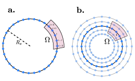
Figure 1: Reference structure and coarse-graining volume $\Omega$. a. Model A : Floppy Swarm, Active particle spaced equally on a ring. Around particle $i$ coarse-graining volume (pink shaded) is defined and consists two left and right neighbours.b. Model B : Rigid Swarm, Active particles equally spaced on a ring (dark blue) surrounded by layer of concentric ghost particles (light blue). Coarse-graining volume (pink shaded) around particle $i$ consists of total $8$ particles.

In this letter, we propose a strategy to produce positionally ordered patterns of drones or robotic agents or “bots” [40, 23, 36] that are robust, do not require velocity sensors or any a priori knowledge of the underlying flow field. Another significant finding of our work is that in certain conditions, statistical properties of the underlying flow field can be obtained, as a co-product, without using any invasive velocity probes. A common approach for studying flow statistics involves point particles that preferentially sample the flow structures or using an extended object such as a polymer if two-point correlations are needed [41, 42, 43, 44, 45, 46, 47, 48, 49]. In atmospheric turbulence, these approaches are inefficient to obtain Eulerian statistics since particles separate quickly from one another due to turbulent diffusion [50]. This knowledge, on the other hand, would be of great help in interpreting wind patterns [51] and weather prediction [52], wind energy generation [53], understanding storms and hurricanes etc.

Consider a system of bots placed in some pattern and embedded in a flowing medium. For specificity and computational simplicity, we consider here point particles placed at equal intervals on a circular ring of radius $R_{s}$ in two dimensions (see Fig. 1). Our analysis is general and unchanged if any other pattern or dimension is chosen. The particles have mass $m$ and are allowed to move within a square box of length $L>>R_{s}$. At any time $t$, the position $\mathbf{r}_{i}$ and velocity $\mathbf{v}_{i}$ of $i^{th}$ particle is determined by the set of Stokes-drag equations [54] with a constant drag coefficient $\gamma$ and in the presence of a background flow field $\mathbf{U}(\mathbf{r}_{i},t)$, viz.

$$\frac{d\mathbf{r}_{i}}{dt} = \mathbf{v}_{i}\hskip 2.0pt,$$ (2)

$$m\frac{d\mathbf{v}_{i}}{dt} = -\gamma\left(\mathbf{v}_{i}-\mathbf{U}(\mathbf{r}_{i},t)\right)+\vec{\mathcal{F}}_{i}\hskip 2.0pt,$$ (4)

Here, $\vec{\mathcal{F}}_{i}$ represents active forces produced by the bots’ own propulsion mechanism. These forces may, in principle be programmed to mimic intra-bot interactions arising from a virtual Hamiltonian. We put $m=1$ for our subsequent analysis. Note that, we assume that the bots are small in comparison to the typical flow structure so that their presence does not significantly alter the flow field $\mathbf{U}(\mathbf{r}_{i},t)$.

Here $\mathbf{U}({\bf r},t)$ is the solution of the Navier-Stokes equations under appropriate boundary conditions and parameters representing fully developed turbulence. To reduce computational cost, however, we use a synthetic, multi-scale, spatio-temporally correlated turbulent-like flow field as described in [55, 56, 57] for most of our results. We also show later that our main conclusions are unchanged if a realistic $\mathbf{U}({\bf r},t)$ obtained using Direct Numerical Simulation (DNS) [58, 59] is used.

The velocity of the field $\mathbf{U}(\mathbf{r},t)$ at any given position and time is obtained from the Fourier series, $\mathbf{U}(\mathbf{r},t)=V_{0}\sum_{n=1}^{N_{k}}\big{[}\mathbf{A}_{n}\cos(\mathbf{k}_{n}\cdot\mathbf{r}+\omega_{n}t)+\mathbf{B}_{n}\sin(\mathbf{k}_{n}\cdot\mathbf{r}+\omega_{n}t)\big{]}.$ Here $N_{k}$ is the total number of Fourier modes included and $V_{0}$ is a dimensionless constant which determines the strength of the field. Also, the Fourier coefficients $\mathbf{A}_{n}$, $\mathbf{B}_{n}$ and distribution of modes $\mathbf{k}_{n}$, $\omega_{n}$ are chosen randomly with the constraint that the velocity field produced is incompressible and the energy spectrum follows Kolmogorov scaling $k^{-5/3}$; see Supplemental Materials (SM) [60].

What is the nature of the forces $\vec{\mathcal{F}}$ needed to maintain the shape of any given pattern (e.g. a ring) in the presence of turbulent field $\mathbf{U}(\mathbf{r},t)$? It is easy to see that the simplest choice viz. nearest neighbor harmonic forces [61, 62, 63, 64, 65], will not work. Local harmonic forces alone cannot guarantee the stability of the global pattern and under the influence of a turbulent velocity field, the polymer quickly intertwines with itself and collapses [60]. Increasing the range of the harmonic forces is ineffective and simply increases the persistence length - with intertwining happening further and further apart unless a large fraction of particles are bonded to each other [66]. This increases the computational and communication overheads for large swarms. An alternative may be to incorporate three-body forces that prefer particular bond angles [67, 68]. Even in the presence of such interactions, the desired pattern may not be the unique ground state [69], and formulating such interactions may become cumbersome for more complex patterns. We describe below an algorithm which solves this problem, guaranteeing a unique global order using forces derived only from configurations of the local particle neighborhood.

We begin by observing that maintaining local particle connectivity guarantees global stability of any pattern, except for overall affine deformations i.e. all translations, rotations, dilations and shears. The pattern is represented by a set of tagged/labelled reference coordinates $\{{\bf R}_{i}\}$ for particles (bots) $i=1\dots N$. Now, any set of particle displacements $\mathbf{u}_{i}={\bf r}_{i}(t)-{\bf R}_{i}$ can be projected onto orthogonal non-affine and affine subspaces [70, 71] by a linear projection operator ${\mathsf{P}}$ that we define shortly. The non-affine part of the displacements involves particle rearrangements and changes the local connectivity of the neighborhood. We show that it is possible to determine time dependent forces $\vec{{\mathcal{F}}}_{i}(t)$ that selectively suppress non-affine displacements and therefore maintain local connectivity [72, 73, 74, 75]. Since computation of $\vec{{\mathcal{F}}}_{i}(t)$ stems from a linear optimization problem, the desired reference structure is guaranteed to be the unique ground state [70, 76]. While detailed discussions of the non-affine projection formalism is given in [70, 76] (see also SM [60]), we briefly recall the main ideas relevant to the present study.

Around each particle $i$, define a neighborhood $\Omega(i)$ consisting of the neighbours of the $i^{th}$ particle. In $d$ dimension for a given coarse-graining volume consisting of $N_{\Omega}\leq N$ particles there exist $d^{2}$ affine and $N_{\Omega}d-d^{2}$ non-affine displacement modes [70, 76]. Clearly, for non-affine displacement modes to exist, $N_{\Omega}$ requires to satisfy the obvious condition $N_{\Omega}>d$. For any generic deformation of $\Omega(i)$, we construct a block column vector $\mathbf{\Delta}$ of size $N_{\Omega}d$ whose elements are $\Delta_{j\alpha}=u_{j}^{\alpha}-u_{i}^{\alpha}=(r_{j}^{\alpha}-r_{i}^{\alpha})-(R_{j}^{\alpha}-R_{i}^{\alpha}),\quad\forall\quad j\in\Omega(i)$, i.e. the $\alpha$-th component of the relative displacement of particles $i$ and $j$. Next we define the linear projection operator ${\mathsf{P}}$ of $\mathbf{\Delta}$ onto non-affine subspace such that non-affine component of displacements is given by $\mathsf{P}\mathbf{\Delta}$ and $\chi_{i}(\{\mathbf{r}\},\{\mathbf{R}\})=\mathbf{\Delta}^{\mathrm{T}}\mathsf{P}\mathbf{\Delta}$ measures total non-affinity associated with the deformed $\Omega(i)$. The projection operator $\mathsf{P}$ is a function only of the reference structure and is given by $\mathsf{P}=\mathsf{I-M(\mathsf{M^{\mathrm{T}}M})^{-1}\mathsf{M}^{\mathrm{T}}}$ with block matrix $\mathsf{M}_{j\alpha,\mu\nu}=\delta_{\alpha\mu}(R_{j}^{\nu}-R_{i}^{\nu})$, where $R_{j}^{\nu},R_{i}^{\nu}$ are $\nu^{th}$ components of the desired reference position of active particles for $j\in\Omega(i)$ [60]. The active forces for the swarm are then defined as $\vec{\mathcal{F}}_{i}=-\partial(-h_{X}NX)/\partial\mathbf{r}_{i}$ where the parameter $h_{X}$ determines the strength of non-affine active forces conjugate to global non-affinity field $X(\{\mathbf{r}\},\{\mathbf{R}\})=N^{-1}\sum_{i}\chi_{i}$. Note that although $X$ is a multiparticle potential, it is fairly short-ranged and only the neighbouring drones within coarse-grained region of a given bot indexed $i$ contributes to the gradient of $X$ (see Fig. 1, Supplemental Material [60] and Fig. S1). In other words, positional information of only the neighbouring drones is required to calculate non-affine forces, resulting in reduced communication and computational cost. By construction, negative values of $h_{X}$ selectively suppress non-affine displacements of the swarm while positive values enhance them. For any desired reference structure, the matrix $\mathsf{P}$ is calculated and uploaded into the memory of drones. At any time $t$, a drone, $i$, can determine the forces $\vec{{\mathcal{F}}}_{i}(t)$ from the known instantaneous positions of its neighbors. Once applied in the form of extra thrust, these forces tend to reduce $X$, and stabilize the pattern.

We introduce two distinct models viz. “Model A” : a floppy swarm and “Model B” : a rigid swarm, see Fig 1. In Model A we use a coarse-graining volume $\Omega$ consisting of four particles viz. two left and right neighbours of the central particle. On the other hand, in Model B, active particle are sandwiched between two concentric rings of “ghost” particles. The position of the particles in the ghost layers are not affected by the turbulent field or non-affine forces and remain virtual, stored only in the memory of robotic agents. These virtual coordinates of ghost particles are free to translate and rotate along with particles of the actual swarm. The ghost particles in this setting satisfy rigid body constraints and therefore their positions are updated by rigid translation and rotations, $\mathbf{r}+\mathbf{V}_{com}\delta t+\Phi\delta t\hat{z}\times(\mathbf{r}-\mathbf{R}_{com})$. Here $\mathbf{R}_{com}$, $\mathbf{V}_{com}$ and $\Phi$ are the centre of mass position, velocity and average angular velocity of the actual swarm. The ghost particle positions are included in the coarse-graining volume $\Omega$ and are taken into account while calculating $\vec{{\mathcal{F}}}_{i}$ for the actual bots. Coarse-graining volume for Model B thus consist of total $8$ particles as shown in Fig 1.

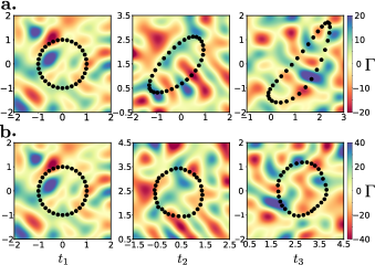
Figure 2: Time evolution ($t_{1}<t_{2}<t_{3}$) of (a.) Model A ($h_{X}=-1000$, $V_{0}=0.5$) and (b.) Model B ($h_{X}=-1$, $V_{0}=1$) respectively. Background color represents the vorticity values ($\Gamma=\nabla\times\mathbf{U}$) of the turbulent field. In Model A, a global transformation of the circular ring to an ellipse is allowed and cost no energy. Model B, on the other hand, is stiffer. Only a portion of the full simulation cell has been shown for clarity.

Time dependent configurations from Model A, shown in Fig. 2a reveals a stable elliptical pattern for sufficiently high values of $h_{X}$. For small $h_{X}$, while the ring may occasionally intertwine with itself, it is guaranteed to disentangle back, in sharp contrast to the harmonic case. Highly elliptical configurations are, however, observed. The transformation that takes a circle to an ellipse is affine and such deformations, no matter how much large, do not produce any non-affinity in the system and are allowed as long as local neighborhood connectivity between particles is preserved. The presence of ghost particles in Model B serves as a “stencil” for the physical swarm and all relative affine deformations of the swarm keeping ghost particles fixed are penalized. The only zero energy cost affine transformations are pure rotations and translations of the system as a whole. Fig. 2b shows typical configurations of a Model B swarm.

It is clear that eddies with sizes much smaller than the size of the swarm cannot affect $\langle X\rangle$. On the other hand, very large eddies simply carry the swarm along introducing mainly affine deformations so that $\langle X\rangle\to 0$. Therefore $\langle X\rangle$ grows with decreasing eddy size saturating to a limit $X_{c}$ for eddies below a cutoff size corresponding to frequency $\omega_{c}$ (see SM [60]). The only two dimensionless quantities are therefore $\langle X\rangle/X_{c}$ and $V_{0}^{2}\gamma\omega_{c}/|h_{X}|$ so that the leading behavior of $\langle X\rangle\sim V_{0}^{2}\gamma/|h_{X}|$ for both Models A and B as shown in Fig. 3. The greater flexibility of Model A implies power expended by non-affine forces is much smaller compared to B as we discuss below.

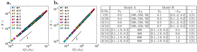
Figure 3: Model A (a.) and Model B (b.): Global non-affinity $\langle X\rangle$ scales linearly with $V_{0}^{2}\gamma/|h_{X}|$. Different symbols represents different combinations of the non-affine field $h_{X}$, $V_{0}$ and $\gamma$ (Stoke’s number). Since global non-affinity measures the non-affine deformation of the swarm, an increase in the value of $X$ as a function of $V_{0}$ indicates the destabilizing tendency of the background flow. On the other hand, counteracting non-affine forces tend to reduce these non-affine deformations and therefore reduce $X$. Table of values of $V_{0}$, $h_{X}$ and $\gamma$ for Models A and B used for generating a&b is also shown. Here the square brackets represents an interval with initial, final, and step values respectively. The parenthesis correspond to different value of $\gamma$.

Note that a constant $\langle X\rangle$ implies zero average power. Indeed, taking a dot product of both sides of the second equation in the set Eq.(4) with the velocity $\mathbf{v}_{i}$ one obtains the rate of change of the kinetic energy ($=0$ in the steady state) as $\vec{{\mathcal{F}}}_{i}\cdot{\mathbf{v}}_{i}-\gamma(v_{i}^{2}-\mathbf{U}(\mathbf{r},t)\cdot{\mathbf{v}}_{i})$. The first term is the power expended by the non-affine forces and if ${\mathbf{v}}_{i}$ follows the local fluid velocity $\mathbf{U}(\mathbf{r},t)$ - true for a swarm drifting along with the fluid medium, this is, on average zero. In practice, the distribution of power expended by $\vec{\mathcal{F}}_{i}$ fluctuates around zero with an error that is much smaller for Model A than for Model B as expected; see SM [60] for a detailed analysis for the specific case of the synthetic turbulent field used in this work.

We end this Letter by demonstrating how the Model B swarm may be used to obtain the statistics of the turbulent flow field $\mathbf{U}(\mathbf{r},t)$

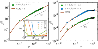
Figure 4: Longitudinal structure function $S^{||}(r)$ as a function of distance $r=|\mathbf{r}_{ij}|$ measured at Eulerian points (solid brown line) and using non-affine forces (colored dots) in Model B. In (a.) $\mathbf{U}({\bf r},t)$ is the same synthetic turbulent field used for earlier calculations. Simulation was done for a ring of radius $R_{s}=2$, box size $L=40$ and for $N=128$ particles. Inset shows linear regression error $\mathcal{E}$ of the obtained non-affine force structure function when compared to the expected $2/3$ law. Note that for a given value of $\gamma$, there exist a range of $|h_{X}|$ for which $\mathcal{E}$ is minimum. (b.) Same as in (a) but for a $\mathbf{U}({\bf r},t)$ obtained from DNS with simulation parameters as $R_{s}=\pi/5$, box size $L=2\pi$ and $N=128$. To highlight the identical scaling, the velocity structure function obtained using the Eulerian flow field (solid brown line) is scaled by a constant prefactor.

over a few meters to kilometers. One may be able to measure the local velocity field using appropriate sensors and compute correlation functions and structure function “on the fly”. While this is of course possible, drone swarms, stabilized using forces which suppress $X$, can go a step further. Specifically, the swarm can be used to obtain equal-time measurements over a wide range of spatial length scales. This is useful to probe fields which involves flow structures at multiple length scales. To see this, we first point out that interestingly, no knowledge of the velocity field is necessary to derive the active forces $\vec{\mathcal{F}}_{i}$. They depend only on $\chi$ and therefore only on the knowledge of the instantaneous and reference positions of the neighbours. Obtaining information about positions is technically far easier than measuring local flow velocities. We calculate the longitudinal structure function [50] for non-affine forces $S_{\mathcal{F}}^{||}(r_{ij})=\langle((\vec{\mathcal{F}}_{i}-\vec{\mathcal{F}}_{j})\cdot\hat{\mathbf{r}}_{ij})^{2}\rangle$ by binning equidistant pairs $r_{ij}$ of drones and averaged over different realisations.

Fig. 4a and b shows the non-affine force structure function together with the Eulerian form computed for our synthetic turbulent field $\mathbf{U}({\bf r},t)$ and the flow field obtained from DNS(see SM [60] for DNS details) respectively. The structure function of the non-affine forces reproduces the Eulerian curve. The presence of ghost layers, implies that all displacement of the bots except for uniform translation and rotations are considered non-affine and are counterbalanced by the restoring non-affine forces. Thus the swarm in Model B is analogous to elastic ring polymer [49] with the rigidity parameter as $|h_{X}|$. However a key difference between a polymer and our swarm is that for zero or very small values of rigidity $|h_{X}|$, the swarm itself is not stable. The significance of $|h_{X}|$ on the stability of patterned swarm and the structure function is motivated by reference [49] and is discussed below.

By looking at the momentum equation for the bots Eq.(4), it is possible to define two characteristic time scales viz. $\tau_{\gamma}=m/\gamma$ and $\tau_{X}=\sqrt{m/|h_{X}|}$; associated with the damping and swarm rigidity. Depending on the ratio of these timescales, various regimes of the swarm exist. For a given background field, the value of $\tau_{\gamma}$ is set by the mass and shape of the bots. For such a system the swarm itself is not stable for too small values of $|h_{X}|$; in contrast to the flexible polymer described in reference [49]. On the other hand, a large value of rigidity ($|h_{X}|$) pushes normal modes of the swarm towards the higher frequencies with either little or no overlap with the frequency spectra of the turbulent field. Drawing analogy to a driven oscillator, the amplitude corresponding to driving frequencies (turbulent frequencies) becomes significantly small such that any fluctuations created by the background field dampen quickly with time scale $\tau_{X}$. The deformation of the swarm is therefore not subject to turbulence. This immediately suggests an optimum value of $|h_{X}|$ for which non-affine forces are proportional to the background velocity field and yields the desired structure function. To identify the optimum value of $|h_{X}|$, we plot (Fig. 4 inset) the linear regression error $\mathcal{E}=\langle(1-S_{\mathcal{F}}^{||}(r)r^{-2/3}/\langle S_{\mathcal{F}}^{||}(r)r^{-2/3}\rangle_{r})^{2}\rangle_{r}$ of the non-affine force structure function obtained compared to the predicted $2/3$ law for various values of $\gamma$ and $|h_{X}|$. The inset of figure 4b clearly shows a range of the optimum value of $|h_{X}|$ for which $\mathcal{E}$ is the minimum and the structure function of the non-affine forces yields the predicted $2/3$ behaviour. Therefore, an imprint of the statistics of $\mathbf{U}(\mathbf{r},t)$ is present in the statistics of the non-affine forces used to stabilize the swarm! Note that large values of $\gamma$ also requires large values of $|h_{X}|$ to stabilise. While of course, this is achievable in simulations, in real-world it is limited by the aerodynamics, design, and capacity of the drones to produce the required thrust.

This surprising result elucidates a very important aspect of the Model B swarm. Since, non-affine forces need to be computed anyway in order to stabilize the structure, no extra measurements are required for obtaining the structure function of the background flow field. The set of robotic agents such as drones can be set up as a Model B swarm to probe the statistics of the atmospheric turbulence at large length scales. It is also easy to make a swarm switch between Model A and Model B modes because the difference is only in the reference configurations. The swarm can, therefore, fly in the floppy mode to conserve energy but switch to a stiffer configuration when a measurement of $S^{||}(r_{ij})$ is needed. .

We thank S. Ganguly, P. Nath, K. Ramola, V. Pandey, and N. Rana for useful discussions. Intra mural support from the Department of Atomic Energy, Government of India is gratefully acknowledged.

P. Popli and P. Perlekar acknowledge the contributions of Surajit Sengupta, now sadly deceased, to the development and completion of this work.

in 1,…,12 See pages \x of SM/SM.pdf

References

- Cavagna and Giardina [2014] A. Cavagna and I. Giardina, Annual Review of Condensed Matter Physics 5, 183 (2014).
- Hildenbrandt, Carere, and Hemelrijk [2010] H. Hildenbrandt, C. Carere, and C. K. Hemelrijk, Behavioral Ecology 21, 1349 (2010).
- Loomis [1987] W. F. Loomis, Methods in Cell Biology 28, 31 (1987).
- Rappel et al. [1999] W. J. Rappel, A. Nicol, A. Sarkissian, H. Levine, and W. F. Loomis, Physical Review Letters 83, 1247 (1999).
- Raper and Bonner [1968] K. B. Raper and J. T. Bonner, Mycologia 60, 211 (1968).
- Reynolds [1987] C. W. Reynolds, in Proceedings of the 14th Annual Conference on Computer Graphics and Interactive Techniques, SIGGRAPH 1987 (Association for Computing Machinery, Inc, 1987) pp. 25–34.
- Huth and Wissel [1990] A. Huth and C. Wissel, The Movement of Fish Schools: A Simulation Model (1990) pp. 577–595.
- Partridge [1982] B. L. Partridge, Scientific American 246, 114 (1982).
- Major [1978] P. F. Major, Animal Behaviour 26, 760 (1978).
- Landeau and Terborgh [1986] L. Landeau and J. Terborgh, Animal Behaviour 34, 1372 (1986).
- Hatwalne et al. [2004] Y. Hatwalne, S. Ramaswamy, M. Rao, and R. A. Simha, Physical Review Letters 92 (2004), 10.1103/PhysRevLett.92.118101.
- Aditi Simha and Ramaswamy [2002] R. Aditi Simha and S. Ramaswamy, Physical review letters 89, 058101 (2002).
- Gazzola et al. [2016] M. Gazzola, A. A. Tchieu, D. Alexeev, A. De Brauer, and P. Koumoutsakos, Journal of Fluid Mechanics 789, 726 (2016).
- Gupta et al. [2020] A. Gupta, A. Roy, A. Saha, and S. S. Ray, Physical Review Fluids 5 (2020), 10.1103/PhysRevFluids.5.052601.
- Simha and Ramaswamy [2002] R. A. Simha and S. Ramaswamy, in Physica A: Statistical Mechanics and its Applications, Vol. 306 (2002) pp. 262–269.
- Toner [2012] J. Toner, Physical Review Letters 108 (2012), 10.1103/PhysRevLett.108.088102.
- Bricard et al. [2013] A. Bricard, J. B. Caussin, N. Desreumaux, O. Dauchot, and D. Bartolo, Nature 503, 95 (2013).
- Geyer, Morin, and Bartolo [2018] D. Geyer, A. Morin, and D. Bartolo, Nature Materials 17, 789 (2018).
- Levine, Rappel, and Cohen [2001] H. Levine, W. J. Rappel, and I. Cohen, Physical Review E - Statistical, Nonlinear, and Soft Matter Physics 63, 1 (2001).
- Wang et al. [2021] G. Wang, T. V. Phan, S. Li, M. Wombacher, J. Qu, Y. Peng, G. Chen, D. I. Goldman, S. A. Levin, R. H. Austin, and L. Liu, Physical Review Letters 126, 108002 (2021).
- Vicsek et al. [1995] T. Vicsek, A. Czirk, E. Ben-Jacob, I. Cohen, and O. Shochet, Physical Review Letters 75, 1226 (1995).
- Czirók, Stanley, and Vicsek [1997] A. Czirók, H. E. Stanley, and T. Vicsek, Journal of Physics A: Mathematical and General 30, 1375 (1997).
- Floreano and Wood [2015] D. Floreano and R. J. Wood, “Science, technology and the future of small autonomous drones,” (2015).
- Alfeo et al. [2018] A. L. Alfeo, M. G. Cimino, N. De Francesco, M. Lega, and G. Vaglini, Journal of Computational Science 29, 19 (2018).
- Tosato et al. [2019] P. Tosato, D. Facinelli, M. Prada, L. Gemma, M. Rossi, and D. Brunelli, in 20th IEEE International Symposium on A World of Wireless, Mobile and Multimedia Networks, WoWMoM 2019 (Institute of Electrical and Electronics Engineers Inc., 2019).
- [26] “US9853715B2 - Broadband access system via drone/UAV platforms - Google Patents,” .
- Mozaffari et al. [2019] M. Mozaffari, W. Saad, M. Bennis, Y. H. Nam, and M. Debbah, IEEE Communications Surveys and Tutorials 21, 2334 (2019).
- Khan, Qureshi, and Khanzada [2019] M. A. Khan, I. M. Qureshi, and F. Khanzada, Drones 3, 1 (2019).
- [29] Google, “Loon,” .
- [30] Space X, “Starlink,” .
- [31] OWL, “Project OWL,” .
- Sinha, Ramaswamy, and Rao [1990] S. Sinha, R. Ramaswamy, and J. S. Rao, Physica D: Nonlinear Phenomena 43, 118 (1990).
- Sinha [1991] S. Sinha, Physics Letters A 156, 475 (1991).
- Kuo and Golnaraghi [2003] B. C. Kuo and M. F. Golnaraghi, Automatic control systems (John Wiley & Sons, 2003) p. 609.
- Majd et al. [2018] A. Majd, A. Ashraf, E. Troubitsyna, and M. Daneshtalab, in Proceedings - 26th Euromicro International Conference on Parallel, Distributed, and Network-Based Processing, PDP 2018 (Institute of Electrical and Electronics Engineers Inc., 2018) pp. 101–108.
- [36] Intel, “Drone Light Shows Powered by Intel,” https://www.intel.in/content/www/in/en/technology-innovation/aerial-technology-light-show.html and https://inteldronelightshows.com/performance/xxiii-olympic-winter-games/.
- Khurana and Ouellette [2013] N. Khurana and N. T. Ouellette, New Journal of Physics 15, 095015 (2013).
- Vásárhelyi et al. [2018] G. Vásárhelyi, C. Virágh, G. Somorjai, T. Nepusz, A. E. Eiben, and T. Vicsek, Science Robotics 3 (2018), 10.1126/scirobotics.aat3536.
- Choudhary, Venkataraman, and Sankar Ray [2015] A. Choudhary, D. Venkataraman, and S. Sankar Ray, EPL 112 (2015), 10.1209/0295-5075/112/24005.
- Elkaim, Pradipta Lie, and Gebre-Egziabher [2015] G. H. Elkaim, F. A. Pradipta Lie, and D. Gebre-Egziabher, in Handbook of Unmanned Aerial Vehicles (Springer Netherlands, 2015).
- Ducasse and Pumir [2008] L. Ducasse and A. Pumir, Physical Review E - Statistical, Nonlinear, and Soft Matter Physics 77 (2008), 10.1103/PhysRevE.77.066304.
- Bandi, Cressman, and Goldburg [2008] M. M. Bandi, J. R. Cressman, and W. I. Goldburg, Journal of Statistical Physics 130, 27 (2008).
- Lalescu and Wilczek [2018] C. C. Lalescu and M. Wilczek, New Journal of Physics 20, 13001 (2018).
- Singh et al. [2020] R. Singh, M. Gupta, J. R. Picardo, D. Vincenzi, and S. S. Ray, Physical Review E 101 (2020), 10.1103/PhysRevE.101.053105.
- Picardo et al. [2018] J. R. Picardo, D. Vincenzi, N. Pal, and S. S. Ray, Physical Review Letters 121 (2018), 10.1103/PhysRevLett.121.244501.
- Ali et al. [2016] A. Ali, E. L. C. V. M. Plan, S. S. Ray, and D. Vincenzi, Physical Review Fluids 1, 82402 (2016).
- Bec [2003] J. Bec, Physics of Fluids 15 (2003), 10.1063/1.1612500.
- Gustavsson and Mehlig [2016] K. Gustavsson and B. Mehlig, Advances in Physics 65, 1 (2016).
- Rosti et al. [2018] M. E. Rosti, A. A. Banaei, L. Brandt, and A. Mazzino, Physical Review Letters 121 (2018), 10.1103/PhysRevLett.121.044501.
- Frisch [1995] U. Frisch, Turbulence (Cambridge University Press, 1995).
- Wang, Lu, and Qiao [2009] C. Wang, Z. Lu, and Y. Qiao, in 1st International Conference on Sustainable Power Generation and Supply, SUPERGEN ’09 (2009).
- Richardson [1922] L. F. Richardson, Weather Prediction by Numerical Process (2nd edition in 2007 with a foreword by Peter Lynch) (Cambridge University Press, 1922) p. 231.
- Bandi [2017] M. M. Bandi, Physical Review Letters 118, 028301 (2017).
- Batchelor [2000] G. K. Batchelor, An Introduction to Fluid Dynamics (Cambridge University Press, 2000).
- Fung and Vassilicos [1998] J. C. Fung and J. C. Vassilicos, Physical Review E - Statistical Physics, Plasmas, Fluids, and Related Interdisciplinary Topics 57, 1677 (1998).
- Fung et al. [1992] J. C. Fung, J. C. Hunt, N. A. Malik, and R. J. Perkins, Journal of Fluid Mechanics 236, 281 (1992).
- Nicolleau and Yu [2004] F. Nicolleau and G. Yu, Physics of Fluids 16, 2309 (2004).
- Perlekar, Pal, and Pandit [2017] P. Perlekar, N. Pal, and R. Pandit, Scientific Reports 7, 44589 (2017).
- Xiao et al. [2009] Z. Xiao, M. Wan, S. Chen, and G. L. Eyink, Journal of Fluid Mechanics 619, 1 (2009).
- [60] Please see Supplementary Material for more details which also includes references [77-79].
- Brouzet, Verhille, and Le Gal [2014] C. Brouzet, G. Verhille, and P. Le Gal, Physical Review Letters 112 (2014), 10.1103/PhysRevLett.112.074501.
- Verhille and Bartoli [2016] G. Verhille and A. Bartoli, Experiments in Fluids 57 (2016), 10.1007/s00348-016-2201-1.
- Gay, Favier, and Verhille [2018] A. Gay, B. Favier, and G. Verhille, EPL 123 (2018), 10.1209/0295-5075/123/24001.
- Dotto and Marchioli [2019] D. Dotto and C. Marchioli, Acta Mechanica 230, 597 (2019).
- Allende, Henry, and Bec [2018] S. Allende, C. Henry, and J. Bec, Physical Review Letters 121 (2018), 10.1103/PhysRevLett.121.154501.
- Maxwell [1864] J. C. Maxwell, The London, Edinburgh, and Dublin Philosophical Magazine and Journal of Science 27, 294 (1864).
- Keating [1966] P. N. Keating, Physical Review 145, 637 (1966).
- Kirkwood [1939] J. G. Kirkwood, The Journal of Chemical Physics 7, 506 (1939).
- Kedia et al. [2019] H. Kedia, D. Pan, J.-J. Slotine, and J. L. England, (2019).
- Ganguly et al. [2013] S. Ganguly, S. Sengupta, P. Sollich, and M. Rao, Physical Review E - Statistical, Nonlinear, and Soft Matter Physics 87, 042801 (2013).
- Ganguly, Sengupta, and Sollich [2015] S. Ganguly, S. Sengupta, and P. Sollich, Soft Matter 11, 4517 (2015).
- Popli, Ganguly, and Sengupta [2017] P. Popli, S. Ganguly, and S. Sengupta, Soft Matter 14, 104 (2017).
- Ganguly et al. [2017] S. Ganguly, P. Nath, J. Horbach, P. Sollich, S. Karmakar, and S. Sengupta, The Journal of Chemical Physics 146, 124501 (2017).
- Ganguly et al. [2018] S. Ganguly, D. Das, J. Horbach, P. Sollich, S. Karmakar, and S. Sengupta, Journal of Chemical Physics 149, 184503 (2018).
- Mitra et al. [2015] A. Mitra, S. Ganguly, S. Sengupta, and P. Sollich, Journal of Statistical Mechanics: Theory and Experiment 2015, P06025 (2015).
- Popli et al. [2019] P. Popli, S. Kayal, P. Sollich, and S. Sengupta, Physical Review E 100, 033002 (2019).
- Grønbech-Jensen and Farago [2013] N. Grønbech-Jensen and O. Farago, Molecular Physics 111, 983 (2013).
- Reddy et al. [2020] V. S. Reddy, P. Nath, J. Horbach, P. Sollich, and S. Sengupta, Physical Review Letters 124, 025503 (2020).
- Nath et al. [2018] P. Nath, S. Ganguly, J. Horbach, P. Sollich, S. Karmakar, and S. Sengupta, Proceedings of the National Academy of Sciences of the United States of America 115, E4322 (2018).