11institutetext: Department of Physics and Astronomy, National Taiwan University, Taipei 10617, Taiwan

The supersymmetric spinning polynomial

Jin-Yu Liu 1 โ€ƒโ€ƒ Zhe-Ming You
Abstract

In this paper, we construct the supersymmetric spinning polynomials. These are orthogonal polynomials that serve as an expansion basis for the residue or discontinuity of four-point scattering amplitudes, respecting four-dimensional super Poincare invariance. The polynomials are constructed by gluing on-shell supersymmetric three-point amplitudes of one massive two massless multiplets, and are identified with algebraic Jacobi-polynomials. Equipped with these we construct the supersymmetric EFThedron, which geometrically defines the allowed region of Wilson coefficients respecting UV unitarity and super Poincare invariance.

1 Introduction

Scattering amplitudes have been a fertile ground for the study of implications of fundamental principles, manifested as constraints on its analytic properties. Itโ€™s utility is often based on being expressible in terms of purely on-shell degrees of freedom. In four-dimension massless theory, this is reflected in the use of spinor-helicity formalism (see 1308.1697 ; 1708.03872 for review). Recently, Arkani-Hamed, Huang and Huang introduced a new on-shell massive spinor helicity formalism 1709.04891 , that manifest the little group covariance of four-dimensional scattering amplitudes. Their supersymmetric extension were further developed by 1902.07204 ; 1810.04694 ; 1902.07205 . For any four-point massless tree-amplitude, its residue can be expanded on an orthogonal polynomial basis, with the precise polynomial depending on the helicity of the external and the spin of exchanged states. For external scalars these are just the Legendre polynomials. For external helicity states, the polynomials are proportional to Algebraic Jacobi Function (AJF) $\mathcal{J}^{\alpha,\beta}_{S}\left(-x\right)$, here referred to as spinning polynomials 1709.04891

Ps{hi}โ€‹(x)=gโ€‹(hi,s)โ€‹๐’ฅsฮฑ,ฮฒโ€‹(โˆ’x),superscriptsubscript๐‘ƒ๐‘ subscriptโ„Ž๐‘–๐‘ฅ๐‘”subscriptโ„Ž๐‘–๐‘ subscriptsuperscript๐’ฅ๐›ผ๐›ฝ๐‘ ๐‘ฅ\boxed{P_{s}^{\{h_{i}\}}(x)=g(h_{i},s)\mathcal{J}^{\alpha,\beta}_{s}\left(-x\right)}\,, (1.1)

where

gโ€‹(hi,s)=๐‘”subscriptโ„Ž๐‘–๐‘ absent\displaystyle g(h_{i},s)= (โˆ’1)s+h1โˆ’h2โˆ’h3โˆ’h4โ€‹(s+ฮฑ)!โ€‹(sโˆ’ฮฑ)!โ€‹(s+ฮฒ)!โ€‹(sโˆ’ฮฒ)!(2โ€‹s)!superscript1๐‘ subscriptโ„Ž1subscriptโ„Ž2subscriptโ„Ž3subscriptโ„Ž4๐‘ ๐›ผ๐‘ ๐›ผ๐‘ ๐›ฝ๐‘ ๐›ฝ2๐‘ \displaystyle(-1)^{s+h_{1}-h_{2}-h_{3}-h_{4}}\frac{\sqrt{\left(s+\alpha\right)!(s-\alpha)!(s+\beta)!(s-\beta)!}}{(2s)!}
๐’ฅsฮฑ,ฮฒโ€‹(โˆ’x)=subscriptsuperscript๐’ฅ๐›ผ๐›ฝ๐‘ ๐‘ฅabsent\displaystyle\mathcal{J}^{\alpha,\beta}_{s}\left(-x\right)= (s+ฮฑ)!โ€‹(sโˆ’ฮฑ)!(s+ฮฒ)!โ€‹(sโˆ’ฮฒ)!โ€‹(1+x2)ฮฑ+ฮฒ2โ€‹(1โˆ’x2)ฮฑโˆ’ฮฒ2ร—Jsโˆ’ฮฑฮฑ+ฮฒ,ฮฑโˆ’ฮฒโ€‹(โˆ’x).๐‘ ๐›ผ๐‘ ๐›ผ๐‘ ๐›ฝ๐‘ ๐›ฝsuperscript1๐‘ฅ2๐›ผ๐›ฝ2superscript1๐‘ฅ2๐›ผ๐›ฝ2subscriptsuperscript๐ฝ๐›ผ๐›ฝ๐›ผ๐›ฝ๐‘ ๐›ผ๐‘ฅ\displaystyle\sqrt{\frac{\left(s+\alpha\right)!(s-\alpha)!}{(s+\beta)!(s-\beta)!}}\left(\frac{1+x}{2}\right)^{\frac{\alpha+\beta}{2}}\left(\frac{1-x}{2}\right)^{\frac{\alpha-\beta}{2}}\times J^{\alpha+\beta,\alpha-\beta}_{s-\alpha}\left(-x\right). (1.2)

x=cโ€‹oโ€‹sโ€‹(ฮธ)๐‘ฅ๐‘๐‘œ๐‘ ๐œƒx=cos(\theta) is scattering angle in center of mass frame thus $-1\leq x\leq 1$. $\alpha=h_{1}-h_{2},\,\beta=h_{3}-h_{4}$ with $h_{i}$ the helicity of external states. The fact that they are expandable on orthogonal polynomials, is a simple reflection of the uniqueness of the three-point amplitude between one massive and two massless legs in four-dimensions. In this paper, we will show that when the theory enjoys super poincare invariance, the residue of the four-point amplitude is expandable on the super polynomials $\mathcal{P}^{H_{i}}_{\mathcal{N},\mathcal{S}}(x,\eta_{i}^{\mathcal{N}})$, each represent the exchange of a spin-$\mathcal{S}$ massive super multiplet. These are nothing but AJF multiplying Grassmann delta function:

๐’ซ๐’ฉ,๐’ฎ{Hi}โ€‹(x,ฮทi๐’ฉ)=m๐’ฉโ€‹ฮด(2โ€‹๐’ฉ)โ€‹(Qโ€ )โ€‹gโ€‹(Hi,๐’ฎ)โ€‹๐’ฅ๐’ฎH1โˆ’H2,H3โˆ’H4โ€‹(โˆ’x),subscriptsuperscript๐’ซsubscript๐ป๐‘–๐’ฉ๐’ฎ๐‘ฅsuperscriptsubscript๐œ‚๐‘–๐’ฉsuperscript๐‘š๐’ฉsuperscript๐›ฟ2๐’ฉsuperscript๐‘„โ€ ๐‘”subscript๐ป๐‘–๐’ฎsubscriptsuperscript๐’ฅsubscript๐ป1subscript๐ป2subscript๐ป3subscript๐ป4๐’ฎ๐‘ฅ\begin{split}&\boxed{\mathcal{P}^{\{H_{i}\}}_{\mathcal{N},\mathcal{S}}(x,\eta_{i}^{\mathcal{N}})=m^{\mathcal{N}}\delta^{(2\mathcal{N})}(Q^{\dagger})g(H_{i},\mathcal{S})\mathcal{J}^{H_{1}-H_{2},H_{3}-H_{4}}_{\mathcal{S}}\left(-x\right)}\end{split}\,, (1.3)

Instead of using $h_{i}$ to label helicity in the spinning polynomials, we use capital $H_{i}$ label the helicity of the super multiplets and $\alpha=H_{1}-H_{2},\,\beta=H_{3}-H_{4}$ here. Note that since both the super and spinning polynomials are expressed on the same basis of AJF, combined with the fact super multiplet decompose onto a sum of components, implies algebraic relation amongst the AJFs. This is precisely given by the recurrence relation of Jacobi polynomial

$$\begin{split}J^{a,b}_{n}(-x)=&\frac{(n+a+b+1)}{(2n+a+b+1)}J^{a+1,b}_{n}(-x)-\frac{(n+b)}{(2n+a+b+1)}J^{a+1,b}_{n-1}(-x).\end{split}$$ (1.4)

An explicit example is shown in the fixing external states on specific component field. We use Grassmann derivative to fix external states and the recurrence relation give us:

$$\begin{split}\frac{\partial}{\partial\eta_{2}}\frac{\partial}{\partial\eta_{4}}\mathcal{P}^{\{H_{i}\}}_{\mathcal{N}=1,\mathcal{S}}(x,\eta_{i})=&m^{2}P^{\{H_{1},H_{2}{-}\frac{1}{2},H_{3},H_{4}{-}\frac{1}{2}\}}_{\mathcal{S}{+}\frac{1}{2}}\left(x\right)\\ &{+}\frac{m^{2}(\mathcal{S}{-}H_{3}{+}H_{4})(\mathcal{S}{-}H_{1}{+}H_{2})}{\left(2\mathcal{S}\right)\left(2\mathcal{S}{+}1\right)}P^{\{H_{1},H_{2}{-}\frac{1}{2},H_{3},H_{4}{-}\frac{1}{2}\}}_{\mathcal{S}{-}\frac{1}{2}}\left(x\right)\,.\end{split}$$ (1.5)

Said in another way, the algebraic relation amongst the AJFs encodes the possible extension of the Poincare group!

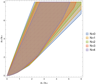
Equipped with the supersymmetric polynomials, we utilize it to constrain the space of EFTs consistent with supersymmetry. As shown in EFThedron , unitarity, locality and Poincare invariance allows us to impose bounds on the coefficients of higher dimension operators of the low energy theory. Poincare invaraince is reflected in the fact that the low energy coefficients are bounded by the convex hull of the derivative expansion of the spinning polynomial. By replacing the latter with supersymmetric polynomial, we obtain new bounds which depends on the number of supersymmetry assumed. We show the bounded region of gluon amplitude in MHV helicity configuration which can be generally expanded as:

A๐’ฉโ€‹(1+,2โˆ’,3+,4โˆ’)|s,tโ‰ชฮ›Uโ€‹V=[13]2โ€‹โŸจ24โŸฉ2โ€‹(asโ€‹t+bs+bt+โˆ‘k,qโ‰ฅ0gk,qโ€‹skโˆ’qโ€‹tq).evaluated-atsuperscript๐ด๐’ฉsuperscript1superscript2superscript3superscript4much-less-than๐‘ ๐‘กsubscriptฮ›๐‘ˆ๐‘‰superscriptdelimited-[]132superscriptdelimited-โŸจโŸฉ242๐‘Ž๐‘ ๐‘ก๐‘๐‘ ๐‘๐‘กsubscript๐‘˜๐‘ž0subscript๐‘”๐‘˜๐‘žsuperscript๐‘ ๐‘˜๐‘žsuperscript๐‘ก๐‘žA^{\mathcal{N}}(1^{+},2^{-},3^{+},4^{-})|_{s,t\ll\Lambda_{UV}}=[13]^{2}\langle 24\rangle^{2}(\frac{a}{st}+\frac{b}{s}{+}\frac{b}{t}+\sum_{k,q\geq 0}g_{k,q}s^{k{-}q}t^{q})\,. (1.6)

The convex hull constrains for $g_{k,q}$ can be found in each $k$ order. We show the constrains for each $g_{k,q}$ in supersymmetry between $\mathcal{N}=0\sim 4$. The result in $k=5$ is in fig.1. It is directly to see, the higher $\mathcal{N}$ supersymmetry will give us the smaller allowed region.

Refer to caption
Figure 1: Cyclic-polytope condition on $(g_{5,1}/g_{5,0},g_{5,2}/g_{5,0})$ with supersymmetry $\mathcal{N}$. We donโ€™t show $g_{5,3},g_{5,4}$ here, it will related to $g_{5,1},g_{5,2}$ by the crossing symmetry $g_{5,i}=g_{5,5-i}$. The bounded region decrease when the superesymmetry $\mathcal{N}$ growth.

This paper is organized as follows. In section 2, we briefly review the spinning polynomials and algebraic Jacobi polynomials. In section 3, we review on-shell $\mathcal{N}=1$ superspace and fix the three-point amplitude with two massless and one massive state consistent with $\mathcal{N}=1$ super Poincare symmetry. We glue two three-point amplitudes and have the residue of $\mathcal{N}=1$ four massless super amplitude. Following the convention of ย 1709.04891 , we transform the result into center of mass frame with scattering angle cโ€‹oโ€‹sโ€‹(ฮธ)๐‘๐‘œ๐‘ ๐œƒcos(\theta) and we have $\mathcal{N}=1$ super polynomial. We decompose super polynomial into spinning polynomials by using recurrence relation of AJF. In section 4, we start from review of $\mathcal{N}=2$ superspace1902.07204 ,then we derive $\mathcal{N}=2$ super polynomial and the general $\mathcal{N}$ super polynomial. Applying super polynomials on EFT, we show the unitary condition on the low energy coefficients in section 5.

2 Review of spinning polynomials

Letโ€™s start from review spinning polynomials which are the expansion basis for the residues/discontinuities of massless four-point amplitude. The residues of the four-point are nothing but product of two three-point amplitudes. In spacetime dimensional four, two massless one massive amplitudes are uniquely fixed by the helicities $h_{1}$, $h_{2}$ of legs 1 and 2, and the spin-s๐‘ s of the massive leg.

$$\begin{split}A(1^{h_{1}},2^{h_{2}},\textbf{P}^{(I_{1}I_{2}\ldots I_{2s})})&=m^{1+h_{1}+h_{2}-s}\langle 12\rangle^{-h_{1}-h_{2}-s}\prod_{t=1}^{h_{1}-h_{2}+s}\langle 2\textbf{P}^{(I_{t}}\rangle\prod_{r=h_{1}-h_{2}+s+1}^{2s}\langle 1\textbf{P}^{I_{r})}\rangle\end{split}$$ (2.1)

The symmetrized SU(2) indices forms the irreducible representation of spin-s๐‘ s state. The powers of $m$ is to ensure the amplitude has the canonical mass dimension in 4d, i.e. 1. Gluing two vertices, we have the residue of four-massless amplitude with exchanging a spin-s๐‘ s state.

$$\begin{split}Res_{s=m^{2}}&[A_{4}(h_{i},s)]=A_{L}(1^{h_{1}},2^{h_{2}},\textbf{P}_{(I_{1}I_{2}\ldots I_{2s})})\cdot A_{R}(3^{h_{3}},4^{h_{4}},-\textbf{P}^{(I_{1}I_{2}\cdots I_{2s})})\\ &=m^{1+h_{1}+h_{2}-s}\langle 12\rangle^{-h_{1}-h_{2}-s}\prod_{t=1}^{h_{1}-h_{2}+s}\langle 2\textbf{P}_{I_{(t}}\rangle\prod_{r=h_{1}-h_{2}+s+1}^{2s}\langle 1\textbf{P}_{I_{r)}}\rangle\\ &\ m^{1+h_{3}+h_{4}-s}\langle 34\rangle^{-h_{3}-h_{4}-s}\prod_{t=1}^{h_{3}-h_{4}+s}\langle 4|-\textbf{P}^{I_{(t}}\rangle\prod_{r=h_{3}-h_{4}+s+1}^{2s}\langle 3|-\textbf{P}^{I_{r)}}\rangle\end{split}$$ (2.2)

We use convention $|{-}\textbf{P}^{I}\rangle=|\textbf{P}^{I}\rangle,\,\,|{-}\textbf{P}^{I}]={-}|\textbf{P}^{I}]$ to denote opposite momentum. The tensor contraction of three-point is done by using identity: $|\textbf{P}_{I}\rangle_{\alpha}\langle\textbf{P}^{I}|^{\beta}=-m_{\textbf{P}}\delta^{\beta}_{\alpha}$. For example, $\left\langle 1\textbf{P}_{I_{r}}\right\rangle$ $\left\langle 3\textbf{P}^{I_{t}}\right\rangle$ can be glued as $\delta^{t}_{r}m_{\textbf{P}}\langle 13\rangle$. Then everything we need to do is summing over all contraction in (2.2). It is easy to show the combinatorial number in the contraction. Assuming one have contracted spinor $|1\rangle$ and $|3\rangle$ "a" times, then we have the spinor bracket with power

{โŸจ13โŸฉ,โŸจ14โŸฉ,โŸจ24โŸฉ,โŸจ23โŸฉ}={a,h2โˆ’h1+sโˆ’a,h1โˆ’h2+h3โˆ’h4+a,h4โˆ’h3+sโˆ’a}.delimited-โŸจโŸฉ13delimited-โŸจโŸฉ14delimited-โŸจโŸฉ24delimited-โŸจโŸฉ23๐‘Žsubscriptโ„Ž2subscriptโ„Ž1๐‘ ๐‘Žsubscriptโ„Ž1subscriptโ„Ž2subscriptโ„Ž3subscriptโ„Ž4๐‘Žsubscriptโ„Ž4subscriptโ„Ž3๐‘ ๐‘Ž\{\langle 13\rangle,\langle 14\rangle,\langle 24\rangle,\langle 23\rangle\}=\{a,h_{2}{-}h_{1}{+}s{-a},h_{1}{-}h_{2}{+}h_{3}{-}h_{4}{+}a,h_{4}{-}h_{3}{+}s{-}a\}. (2.3)

Then we can write down the combinatorial number for each spinor brackets:

$\displaystyle\left\langle 13\right\rangle^{a}$ :(s+h2โˆ’h1a)ร—(s+h4โˆ’h3a)ร—a!:absent๐‘ subscriptโ„Ž2subscriptโ„Ž1missing-subexpression๐‘Žmissing-subexpression๐‘ subscriptโ„Ž4subscriptโ„Ž3missing-subexpression๐‘Žmissing-subexpression๐‘Ž\displaystyle:\left(\begin{array}[]{cr}s+h_{2}-h_{1}&\\ a\end{array}\right)\times\left(\begin{array}[]{cr}s+h_{4}-h_{3}&\\ a\end{array}\right)\times a!\, (2.8)
โŸจ14โŸฉ(h2โˆ’h1+sโˆ’a)superscriptdelimited-โŸจโŸฉ14subscriptโ„Ž2subscriptโ„Ž1๐‘ ๐‘Ž\displaystyle\left\langle 14\right\rangle^{(h_{2}-h_{1}+s-a)} :(h3โˆ’h4+sh2โˆ’h1+sโˆ’a)ร—(h2โˆ’h1+sโˆ’a)!:absentsubscriptโ„Ž3subscriptโ„Ž4๐‘ missing-subexpressionsubscriptโ„Ž2subscriptโ„Ž1๐‘ ๐‘Žmissing-subexpressionsubscriptโ„Ž2subscriptโ„Ž1๐‘ ๐‘Ž\displaystyle:\left(\begin{array}[]{cr}h_{3}-h_{4}+s&\\ h_{2}-h_{1}+s-a\end{array}\right)\times(h_{2}-h_{1}+s-a)!\, (2.11)
$\displaystyle\left\langle 24\right\rangle^{(h_{1}-h_{2}+h_{3}-h_{4}+a)}$ :(h1โˆ’h2+sh1โˆ’h2+h3โˆ’h4+a)ร—(h1โˆ’h2+h3โˆ’h4+a)!:absentsubscriptโ„Ž1subscriptโ„Ž2๐‘ missing-subexpressionsubscriptโ„Ž1subscriptโ„Ž2subscriptโ„Ž3subscriptโ„Ž4๐‘Žmissing-subexpressionsubscriptโ„Ž1subscriptโ„Ž2subscriptโ„Ž3subscriptโ„Ž4๐‘Ž\displaystyle:\left(\begin{array}[]{cr}h_{1}-h_{2}+s&\\ h_{1}-h_{2}+h_{3}-h_{4}+a\end{array}\right)\times(h_{1}-h_{2}+h_{3}-h_{4}+a)!\, (2.14)
โŸจ23โŸฉ(h4โˆ’h3+sโˆ’a)superscriptdelimited-โŸจโŸฉ23subscriptโ„Ž4subscriptโ„Ž3๐‘ ๐‘Ž\displaystyle\left\langle 23\right\rangle^{(h_{4}-h_{3}+s-a)} :(h4โˆ’h3+sโˆ’a)!.:absentsubscriptโ„Ž4subscriptโ„Ž3๐‘ ๐‘Ž\displaystyle:(h_{4}-h_{3}+s-a)!\,. (2.15)

Summing over "a", we have the contraction result in (2.2). It can be

Rโ€‹eโ€‹ss=m2[A4โ€‹(hi,s)]=โˆ‘am2โˆ’2โ€‹s+โˆ‘i(hi)(2โ€‹s)!โ€‹(h1โˆ’h2+s)!โ€‹(h2โˆ’h1+s)!โ€‹(h3โˆ’h4+s)!โ€‹(h4โˆ’h3+s)!(a)!โ€‹(sโˆ’h1+h2โˆ’a)!โ€‹(sโˆ’h3+h4โˆ’a)!โ€‹(h1โˆ’h2+h3โˆ’h4+a)!ร—โŸจ12โŸฉโˆ’h1โˆ’h2โˆ’sโ€‹โŸจ34โŸฉโˆ’h3โˆ’h4โˆ’sโ€‹โŸจ13โŸฉaโ€‹โŸจ14โŸฉsโˆ’h1+h2โˆ’aโ€‹โŸจ24โŸฉh1โˆ’h2+h3โˆ’h4+aโ€‹โŸจ23โŸฉh4โˆ’h3+sโˆ’a.๐‘…๐‘’subscript๐‘ ๐‘ superscript๐‘š2delimited-[]subscript๐ด4subscriptโ„Ž๐‘–๐‘ subscript๐‘Žsuperscript๐‘š22๐‘ subscript๐‘–subscriptโ„Ž๐‘–2๐‘ subscriptโ„Ž1subscriptโ„Ž2๐‘ subscriptโ„Ž2subscriptโ„Ž1๐‘ subscriptโ„Ž3subscriptโ„Ž4๐‘ subscriptโ„Ž4subscriptโ„Ž3๐‘ ๐‘Ž๐‘ subscriptโ„Ž1subscriptโ„Ž2๐‘Ž๐‘ subscriptโ„Ž3subscriptโ„Ž4๐‘Žsubscriptโ„Ž1subscriptโ„Ž2subscriptโ„Ž3subscriptโ„Ž4๐‘Žsuperscriptdelimited-โŸจโŸฉ12subscriptโ„Ž1subscriptโ„Ž2๐‘ superscriptdelimited-โŸจโŸฉ34subscriptโ„Ž3subscriptโ„Ž4๐‘ superscriptdelimited-โŸจโŸฉ13๐‘Žsuperscriptdelimited-โŸจโŸฉ14๐‘ subscriptโ„Ž1subscriptโ„Ž2๐‘Žsuperscriptdelimited-โŸจโŸฉ24subscriptโ„Ž1subscriptโ„Ž2subscriptโ„Ž3subscriptโ„Ž4๐‘Žsuperscriptdelimited-โŸจโŸฉ23subscriptโ„Ž4subscriptโ„Ž3๐‘ ๐‘Ž\begin{split}Res_{s=m^{2}}&[A_{4}(h_{i},s)]=\\ &\sum_{a}\frac{m^{2-2s+\sum_{i}(h_{i})}}{(2s)!}\frac{(h_{1}-h_{2}+s)!(h_{2}-h_{1}+s)!(h_{3}-h_{4}+s)!(h_{4}-h_{3}+s)!}{(a)!(s-h_{1}+h_{2}-a)!(s-h_{3}+h_{4}-a)!(h_{1}-h_{2}+h_{3}-h_{4}+a)!}\\ &\times\left\langle 12\right\rangle^{-h_{1}-h_{2}-s}\left\langle 34\right\rangle^{-h_{3}-h_{4}-s}\langle 13\rangle^{a}\langle 14\rangle^{s-h_{1}+h_{2}-a}\langle 24\rangle^{h_{1}-h_{2}+h_{3}-h_{4}+a}\langle 23\rangle^{h_{4}-h_{3}+s-a}.\end{split} (2.16)

Since the power of spinor brackets are positive integer or zero, the summation is restricted to the region

aโ‰ฅ0,sโˆ’h1+h2โˆ’aโ‰ฅ0,sโˆ’h3+h4โˆ’aโ‰ฅ0,h1โˆ’h2+h3โˆ’h4+aโ‰ฅ0.formulae-sequence๐‘Ž0formulae-sequence๐‘ subscriptโ„Ž1subscriptโ„Ž2๐‘Ž0formulae-sequence๐‘ subscriptโ„Ž3subscriptโ„Ž4๐‘Ž0subscriptโ„Ž1subscriptโ„Ž2subscriptโ„Ž3subscriptโ„Ž4๐‘Ž0a\geq 0,\quad s-h_{1}+h_{2}-a\geq 0,\quad s-h_{3}+h_{4}-a\geq 0,\quad h_{1}-h_{2}+h_{3}-h_{4}+a\geq 0. (2.17)

It is useful to convert spinor brackets into scattering angle x=cโ€‹oโ€‹sโ€‹ฮธ๐‘ฅ๐‘๐‘œ๐‘ ๐œƒx=cos\,\theta in the center of mass frame. The transformation rule can be found in appendix A. As a result, the spinning polynomial is

Rโ€‹eโ€‹ss=m2โ€‹[A4โ€‹(hi,s)]โ‰กPs{hi}โ€‹(x)=gโ€‹(hi,s)โ€‹๐’ฅsฮฑ,ฮฒโ€‹(โˆ’x)๐‘…๐‘’subscript๐‘ ๐‘ superscript๐‘š2delimited-[]subscript๐ด4subscriptโ„Ž๐‘–๐‘ superscriptsubscript๐‘ƒ๐‘ subscriptโ„Ž๐‘–๐‘ฅ๐‘”subscriptโ„Ž๐‘–๐‘ subscriptsuperscript๐’ฅ๐›ผ๐›ฝ๐‘ ๐‘ฅRes_{s=m^{2}}[A_{4}(h_{i},s)]\equiv P_{s}^{\{h_{i}\}}(x)=g(h_{i},s)\mathcal{J}^{\alpha,\beta}_{s}\left(-x\right) (2.18)

where

gโ€‹(hi,s)=๐‘”subscriptโ„Ž๐‘–๐‘ absent\displaystyle g(h_{i},s)= (โˆ’1)s+h1โˆ’h2โˆ’h3โˆ’h4โ€‹(s+ฮฑ)!โ€‹(sโˆ’ฮฑ)!โ€‹(s+ฮฒ)!โ€‹(sโˆ’ฮฒ)!(2โ€‹s)!superscript1๐‘ subscriptโ„Ž1subscriptโ„Ž2subscriptโ„Ž3subscriptโ„Ž4๐‘ ๐›ผ๐‘ ๐›ผ๐‘ ๐›ฝ๐‘ ๐›ฝ2๐‘ \displaystyle(-1)^{s+h_{1}-h_{2}-h_{3}-h_{4}}\frac{\sqrt{\left(s+\alpha\right)!(s-\alpha)!(s+\beta)!(s-\beta)!}}{(2s)!}
๐’ฅsฮฑ,ฮฒโ€‹(โˆ’x)=subscriptsuperscript๐’ฅ๐›ผ๐›ฝ๐‘ ๐‘ฅabsent\displaystyle\mathcal{J}^{\alpha,\beta}_{s}\left(-x\right)= (s+ฮฑ)!โ€‹(sโˆ’ฮฑ)!(s+ฮฒ)!โ€‹(sโˆ’ฮฒ)!โ€‹(1+x2)ฮฑ+ฮฒ2โ€‹(1โˆ’x2)ฮฑโˆ’ฮฒ2ร—Jsโˆ’ฮฑฮฑ+ฮฒ,ฮฑโˆ’ฮฒโ€‹(โˆ’x)๐‘ ๐›ผ๐‘ ๐›ผ๐‘ ๐›ฝ๐‘ ๐›ฝsuperscript1๐‘ฅ2๐›ผ๐›ฝ2superscript1๐‘ฅ2๐›ผ๐›ฝ2subscriptsuperscript๐ฝ๐›ผ๐›ฝ๐›ผ๐›ฝ๐‘ ๐›ผ๐‘ฅ\displaystyle\sqrt{\frac{\left(s+\alpha\right)!(s-\alpha)!}{(s+\beta)!(s-\beta)!}}\left(\frac{1+x}{2}\right)^{\frac{\alpha+\beta}{2}}\left(\frac{1-x}{2}\right)^{\frac{\alpha-\beta}{2}}\times J^{\alpha+\beta,\alpha-\beta}_{s-\alpha}\left(-x\right)
$\displaystyle-1\leq x\leq 1.$ (2.19)

Here $\alpha,\beta$ define as $\alpha=h_{1}-h_{2},\beta=h_{3}-h_{4}$.

Note that the spin-s๐‘ s must satisfy sโ‰ฅโˆฃh1โˆ’h2โˆฃ๐‘ delimited-โˆฃโˆฃsubscriptโ„Ž1subscriptโ„Ž2s\geq\mid h_{1}-h_{2}\mid and {s,h1โˆ’h2}๐‘ subscriptโ„Ž1subscriptโ„Ž2\{s,h_{1}-h_{2}\} must be all integer or half-integer. ๐’ฅsฮฑ,ฮฒsubscriptsuperscript๐’ฅ๐›ผ๐›ฝ๐‘ \mathcal{J}^{\alpha,\beta}_{s} is Algebraic Jacobi Function(AJF) which satisfy orthogonality condition

โˆซโˆ’11๐‘‘xโ€‹๐’ฅsฮฑ,ฮฒโ€‹(x)โ€‹๐’ฅsโ€ฒฮฑ,ฮฒโ€‹(x)=โˆซโˆ’11๐‘‘xโ€‹(1โˆ’x)ฮฑโ€‹(1+x)ฮฒโ€‹Jsฮฑ,ฮฒโ€‹(x)โ€‹Jsโ€ฒฮฑ,ฮฒโ€‹(x)=12โ€‹s+1โ€‹ฮดsโ€‹sโ€ฒ.superscriptsubscript11differential-d๐‘ฅsuperscriptsubscript๐’ฅ๐‘ ๐›ผ๐›ฝ๐‘ฅsuperscriptsubscript๐’ฅsuperscript๐‘ โ€ฒ๐›ผ๐›ฝ๐‘ฅsuperscriptsubscript11differential-d๐‘ฅsuperscript1๐‘ฅ๐›ผsuperscript1๐‘ฅ๐›ฝsubscriptsuperscript๐ฝ๐›ผ๐›ฝ๐‘ ๐‘ฅsubscriptsuperscript๐ฝ๐›ผ๐›ฝsuperscript๐‘ โ€ฒ๐‘ฅ12๐‘ 1subscript๐›ฟ๐‘ superscript๐‘ โ€ฒ\begin{array}[]{lll}\int_{-1}^{1}dx\,\,\mathcal{J}_{s}^{\alpha,\beta}(x)\mathcal{J}_{s^{\prime}}^{\alpha,\beta}(x)=\int_{-1}^{1}dx\,\,(1-x)^{\alpha}(1+x)^{\beta}J^{\alpha,\beta}_{s}(x)J^{\alpha,\beta}_{s^{\prime}}(x)&=&\frac{1}{2s+1}\delta_{s\,s^{\prime}}.\end{array} (2.20)

The advantage of using AJF as opposed to Jacobi-polynomial is the fact that they satisfy the same orthogonality condition as Legendre polynomials. Said in anotherway, using AJF is equivalent to taking into account the fact that the residue has a universal prefactor that is determined by the external helicities. This relation can be translated to the spinning polynomials

โˆซโˆ’11๐‘‘xโ€‹Pshiโ€‹(x)โ€‹Psโ€ฒhiโ€‹(x)=ฮดsโ€‹sโ€ฒ2โ€‹s+1โ€‹(s+ฮฑ)!โ€‹(sโˆ’ฮฑ)!โ€‹(s+ฮฒ)!โ€‹(sโˆ’ฮฒ)!((2โ€‹s)!)2.superscriptsubscript11differential-d๐‘ฅsuperscriptsubscript๐‘ƒ๐‘ subscriptโ„Ž๐‘–๐‘ฅsuperscriptsubscript๐‘ƒsuperscript๐‘ โ€ฒsubscriptโ„Ž๐‘–๐‘ฅsubscript๐›ฟ๐‘ superscript๐‘ โ€ฒ2๐‘ 1๐‘ ๐›ผ๐‘ ๐›ผ๐‘ ๐›ฝ๐‘ ๐›ฝsuperscript2๐‘ 2\begin{split}\begin{array}[]{lll}\int_{-1}^{1}dx\,P_{s}^{h_{i}}(x)\,\,P_{s^{\prime}}^{h_{i}}(x)&=&\frac{\delta_{s\,s^{\prime}}}{2s+1}\frac{\left(s+\alpha\right)!(s-\alpha)!(s+\beta)!(s-\beta)!}{\left((2s)!\right)^{2}}.\end{array}\end{split} (2.21)

3 $\mathcal{N}=1$ Supersymmetry

In this section, we give a brief review of on-shell superspace and superfields. This will allow us to fix the 3-point super amplitude, after which one simply follows the previous example of spinning polynomials: gluing three-point to obtain the super polynomials.

3.1 Review of $\mathcal{N}=1$ super space

We will begin with $\mathcal{N}=1$, the generalization to extended $\mathcal{N}$ are straight forward. Following the convention of 1902.07204 and 0808.1446 , the SUSY generators can be completely written in terms of on-shell variables by introducing grassmann odd variables $\eta$. For example the massive supercharge are

qaห™=ฮป~aห™โ€‹Iโ€‹โˆ‚โˆ‚ฮทI,qaโ€ =ฮปaIโ€‹ฮทI.\begin{split}q_{\dot{a}}=\tilde{\lambda}_{\dot{a}I}\frac{\partial}{\partial\eta_{I}}\,,\quad q^{\dagger}_{a}=\lambda_{a}^{I}\eta_{I}.\end{split} (3.1)

For massless case, this reduces to

qaห™=ฮป~aห™โ€‹โˆ‚โˆ‚ฮท,qaโ€ =ฮปaโ€‹ฮท.\begin{split}q_{\dot{a}}=\tilde{\lambda}_{\dot{a}}\frac{\partial}{\partial\eta}\,,\quad q^{\dagger}_{a}=\lambda_{a}\eta.\end{split} (3.2)

Supergenerators satisfy super algebra relations, {qaห™,qaโ€ }=Paโ€‹aห™subscript๐‘žห™๐‘Žsuperscriptsubscript๐‘ž๐‘Žโ€ subscriptP๐‘Žห™๐‘Ž\{q_{\dot{a}},q_{a}^{\dagger}\}=\textbf{P}_{a\dot{a}}. For on-shell SUSY representation, we introduce on-shell superfields whose $\eta$ expansion gives the component degrees of freedom. For example, a massive spin-$S$ $\mathcal{N}{=}1$ multiplet can be written as

$$\begin{split}\mathcal{S}^{(I_{1}\ldots I_{2S})}&=\phi^{(I_{1}\ldots I_{2S})}+\eta_{J}\Psi^{J(I_{1}\ldots I_{2S})}-\frac{1}{2}\eta_{J}\eta^{J}\tilde{\phi}^{(I_{1}\ldots I_{2S})}\,,\end{split}$$ (3.3)

where the $(I_{1}\cdots I_{2S})$ denote $\frac{I_{1}I_{2}\cdots I_{2S}+I_{2}I_{1}\cdots I_{2S}+\cdots}{(2S)!}$. Each order on the expansion gives different spin states with the same mass. The component field $\Psi^{J(I_{1}\ldots I_{2S})}$ can be separated into irreducible representation by systematically symmetrizing and anti-symmetrizing the free index J with $(I_{1}\cdots I_{2S})$. This leads to $\Psi^{(JI_{1}\ldots I_{2S})}$ and $\Psi_{L}^{\,\,(LI_{2}\ldots I_{2S})}$ representing spin-$S\pm\frac{1}{2}$ states

$$\Psi^{J(I_{1}\ldots I_{2S})}=\Psi^{(JI_{1}\ldots I_{2S})}+\frac{1}{(2S+1)}\sum_{k=1}^{2S}\epsilon^{JI_{k}}\Psi_{L}^{\,\,(LI_{1}\ldots I_{k-1}I_{k+1}\ldots I_{2S})}\,.$$ (3.4)

We can derive the component degrees of freedom from (3.3)

$\displaystyle\phi^{(I_{1}\ldots I_{2S})}$ $\displaystyle=\mathcal{S}^{(I_{1}\ldots I_{2S})}\mid_{\eta=0}$
$\displaystyle\Psi^{J(I_{1}\ldots I_{2S})}$ $\displaystyle=\frac{\partial}{\partial\eta_{J}}\mathcal{S}^{(I_{1}\ldots I_{2S})}\mid_{\eta=0}$
$\displaystyle\tilde{\phi}^{(I_{1}\ldots I_{2S})}$ $\displaystyle=\frac{1}{2}\frac{\partial}{\partial\eta_{J}}\frac{\partial}{\partial\eta^{J}}\mathcal{S}^{(I_{1}\ldots I_{2S})}\mid_{\eta=0}\,.$ (3.5)

For massless multiplet, we instead have

$$\Phi^{H_{i}}=\phi^{H_{i}}+\eta\psi^{H_{i}-\frac{1}{2}}\,,$$ (3.6)

where $\eta$ carries $+\frac{1}{2}$ helicity.

$\mathcal{N}=1$ three-point amplitudes
We now consider the three-point super amplitude for the scattering of $H_{1}$, $H_{2}$ massless and a spin-$S$ massive multiplet, $\mathcal{A}(\Phi_{1}^{H_{1}},\Phi_{1}^{H_{1}},S_{\textbf{p}}^{(I_{1}\ldots I_{2S})})$. The constraint on $\mathcal{A}$ includes it must have $H_{1}$, $H_{2}$ helicity weight, carry (I1โ€‹โ€ฆโ€‹I2โ€‹s)subscript๐ผ1โ€ฆsubscript๐ผ2๐‘ (I_{1}\ldots I_{2s}) symmetrised indices, and satisfy the supersymmetry Ward identities

Qaโ€ โ€‹๐’œโ€‹(ฮฆ1H1,ฮฆ2H2,๐’ฎP(I1โ€‹โ€ฆโ€‹I2โ€‹S))=Qaห™โ€‹๐’œโ€‹(ฮฆ1H1,ฮฆ2H2,๐’ฎP(I1โ€‹โ€ฆโ€‹I2โ€‹S))=0subscriptsuperscript๐‘„โ€ ๐‘Ž๐’œsuperscriptsubscriptฮฆ1subscript๐ป1superscriptsubscriptฮฆ2subscript๐ป2superscriptsubscript๐’ฎPsubscript๐ผ1โ€ฆsubscript๐ผ2๐‘†subscript๐‘„ห™๐‘Ž๐’œsuperscriptsubscriptฮฆ1subscript๐ป1superscriptsubscriptฮฆ2subscript๐ป2superscriptsubscript๐’ฎPsubscript๐ผ1โ€ฆsubscript๐ผ2๐‘†0Q^{\dagger}_{a}\,\mathcal{A}(\Phi_{1}^{H_{1}},\Phi_{2}^{H_{2}},\mathcal{S}_{\textbf{P}}^{(I_{1}\ldots I_{2S})})=Q_{\dot{a}}\,\mathcal{A}(\Phi_{1}^{H_{1}},\Phi_{2}^{H_{2}},\mathcal{S}_{\textbf{P}}^{(I_{1}\ldots I_{2S})})=0 (3.7)

where

Qaโ€ =ฮป1,aโ€‹ฮท1+ฮป2,aโ€‹ฮท2+ฮปp,aIโ€‹ฮทPโ€‹I.subscriptsuperscript๐‘„โ€ ๐‘Žsubscript๐œ†1๐‘Žsubscript๐œ‚1subscript๐œ†2๐‘Žsubscript๐œ‚2subscriptsuperscript๐œ†๐ผp๐‘Žsubscript๐œ‚P๐ผQ^{\dagger}_{a}=\lambda_{1,a}\eta_{1}+\lambda_{2,a}\eta_{2}+\lambda^{I}_{\textbf{p},a}\eta_{\textbf{P}I}\,. (3.8)

Since Qaโ€ superscriptsubscript๐‘„๐‘Žโ€ Q_{a}^{\dagger} is a multiplicative generator, the amplitude must be proportional to to $\delta^{2}(Q)$

๐’œ=ฮด(2)โ€‹(Qโ€ )โ€‹fโ€‹(ฮป,ฮป~,ฮท),๐’œsuperscript๐›ฟ2superscript๐‘„โ€ ๐‘“๐œ†~๐œ†๐œ‚\mathcal{A}=\delta^{(2)}(Q^{\dagger})f(\lambda,\tilde{\lambda},\eta)\,, (3.9)

where

ฮด(2)โ€‹(Qโ€ )=(โŸจi|โ€‹ฮทi+โŸจj|โ€‹ฮทj+โŸจPI|โ€‹ฮทPโ€‹I)โ€‹(|iโŸฉโ€‹ฮทi+|jโŸฉโ€‹ฮทj+|PIโŸฉโ€‹ฮทPโ€‹I)=โŸจ12โŸฉโ€‹ฮท1โ€‹ฮท2+โŸจ1โ€‹PIโŸฉโ€‹ฮท1โ€‹ฮทPโ€‹I+โŸจ2โ€‹PIโŸฉโ€‹ฮท2โ€‹ฮทPโ€‹I+m2โ€‹ฮทPโ€‹Iโ€‹ฮทPI.superscript๐›ฟ2superscript๐‘„โ€ bra๐‘–subscript๐œ‚๐‘–bra๐‘—subscript๐œ‚๐‘—brasuperscriptP๐ผsubscript๐œ‚๐‘ƒ๐ผket๐‘–subscript๐œ‚๐‘–ket๐‘—subscript๐œ‚๐‘—ketsubscriptP๐ผsuperscript๐œ‚๐‘ƒ๐ผdelimited-โŸจโŸฉ12subscript๐œ‚1subscript๐œ‚2delimited-โŸจโŸฉ1superscriptP๐ผsubscript๐œ‚1subscript๐œ‚๐‘ƒ๐ผdelimited-โŸจโŸฉ2superscriptP๐ผsubscript๐œ‚2subscript๐œ‚๐‘ƒ๐ผ๐‘š2subscript๐œ‚๐‘ƒ๐ผsuperscriptsubscript๐œ‚๐‘ƒ๐ผ\begin{split}\delta^{(2)}(Q^{\dagger})=\left(\langle i|\eta_{i}+\langle j|\eta_{j}+\langle\textbf{P}^{I}|\eta_{PI}\right)\left(|i\rangle\eta_{i}+|j\rangle\eta_{j}+|\textbf{P}_{I}\rangle\eta^{PI}\right)\\ =\langle 12\rangle\eta_{1}\eta_{2}+\langle 1\textbf{P}^{I}\rangle\eta_{1}\eta_{PI}+\langle 2\textbf{P}^{I}\rangle\eta_{2}\eta_{PI}+\frac{m}{2}\eta_{PI}\eta_{P}^{I}\,.\end{split} (3.10)

One can then easily check with the momentum conservation

Qโ€‹ฮด(2)โ€‹(Qโ€ )=0.๐‘„superscript๐›ฟ2superscript๐‘„โ€ 0Q\delta^{(2)}(Q^{\dagger})=0\,. (3.11)

The degree in $\eta$ of $f(\lambda,\tilde{\lambda},\eta)$ for general $\mathcal{N}$ and n-point amplitude is given by

$$[f]\leq(n-3)\mathcal{N}\,.$$ (3.12)

Since $n=3$, $f(\lambda,\tilde{\lambda},\eta)$ is purely bosonic. Then we have1902.07204

๐’œโ€‹(ฮฆ1H1,ฮฆ2H2,๐’ฎP(I1,โ€ฆ,I2โ€‹S))=ฮด(2)โ€‹(Qโ€ )โ€‹mH1+H2โˆ’๐’ฎโ€‹โŸจ12โŸฉโˆ’H1โˆ’H2โˆ’๐’ฎโ€‹โˆt=1H1โˆ’H2+๐’ฎโŸจ2โ€‹P(ItโŸฉโ€‹โˆr=H1โˆ’H2+๐’ฎ+12โ€‹๐’ฎโŸจ1โ€‹PIr)โŸฉ.\begin{split}\mathcal{A}(\Phi_{1}^{H_{1}},\Phi_{2}^{H_{2}},\mathcal{S}_{\textbf{P}}^{(I_{1},\ldots,I_{2S})})&=\delta^{(2)}(Q^{\dagger})m^{H_{1}+H_{2}-\mathcal{S}}\langle 12\rangle^{-H_{1}-H_{2}-\mathcal{S}}\prod_{t=1}^{H_{1}-H_{2}+\mathcal{S}}\langle 2\textbf{P}^{(I_{t}}\rangle\prod_{r=H_{1}-H_{2}+\mathcal{S}+1}^{2\mathcal{S}}\langle 1\textbf{P}^{I_{r})}\rangle\end{split}. (3.13)

Itsโ€™ component amplitudes can be extracted by Grassmann derivative. As an example, we show the component amplitude with helicity $H_{1}{-}\frac{1}{2}$ and $H_{2}$ on the massless states. There are four states in the massive multiplet and we choose $\Psi^{(I_{1}\ldots I_{2S}J)},\Theta^{I_{1}\ldots I_{2S}J}$ which both are coming from mixed field $\Psi^{J(I_{1}\ldots I_{2S})}$. Since we are considering mixed field here, we first derive the component amplitude:

$$\begin{split}A(\psi^{H_{1}-\frac{1}{2}},\phi^{H_{2}},\Psi_{\textbf{P}}^{J(I_{1},\ldots,I_{2S})})&=\frac{\partial}{\partial\eta_{1}}\frac{\partial}{\partial\eta_{PJ}}\mathcal{A}(\Phi^{H_{1}},\Phi^{H_{2}},\mathcal{S}_{\textbf{P}}^{(I_{1},\ldots,I_{2S})})\\ &=\langle 1\textbf{P}^{J}\rangle m^{H_{1}+H_{2}-\mathcal{S}}\langle 12\rangle^{-H_{1}-H_{2}-\mathcal{S}}\prod_{t=1}^{H_{1}-H_{2}+\mathcal{S}}\langle 2\textbf{P}^{(I_{t}}\rangle\prod_{r=H_{1}-H_{2}+\mathcal{S}+1}^{2\mathcal{S}}\langle 1\textbf{P}^{I_{r})}\rangle.\end{split}$$ (3.14)

The mixed field in (3.14) can further decompose onto spin-$\mathcal{S}\pm\frac{1}{2}$ by symmetrizing the SU(2) indices

$$\begin{split}&A(\psi^{H_{1}-\frac{1}{2}},\phi^{H_{2}},\Psi_{\textbf{P}}^{(I_{1},\ldots,I_{2S}J)})=m^{H_{1}+H_{2}-\mathcal{S}}\langle 12\rangle^{-H_{1}-H_{2}-\mathcal{S}}\prod_{t=1}^{H_{1}-H_{2}+\mathcal{S}}\langle 2\textbf{P}^{(I_{t}}\rangle\prod_{r=H_{1}-H_{2}+\mathcal{S}+1}^{2\mathcal{S}+1}\langle 1\textbf{P}^{I_{r})}\rangle\\ &A(\psi^{H_{1}-\frac{1}{2}},\phi^{H_{2}},\Theta_{\textbf{P}}^{I_{1}\ldots I_{2S}J})=m^{H_{1}+H_{2}-\mathcal{S}}\langle 12\rangle^{-H_{1}-H_{2}-\mathcal{S}}\\ &\times[\langle 1\textbf{P}^{J}\rangle\prod_{t=1}^{H_{1}-H_{2}+\mathcal{S}}\langle 2\textbf{P}^{(I_{t}}\rangle\prod_{r=H_{1}-H_{2}+\mathcal{S}+1}^{2\mathcal{S}}\langle 1\textbf{P}^{I_{r})}\rangle-\prod_{t=1}^{H_{1}-H_{2}+\mathcal{S}}\langle 2\textbf{P}^{(I_{t}}\rangle\prod_{r=H_{1}-H_{2}+\mathcal{S}+1}^{2\mathcal{S}+1}\langle 1\textbf{P}^{I_{r})}\rangle].\end{split}$$ (3.15)

3.2 The N=1 super polynomial

With the unique three-point super amplitude, we start to construct the basis for 4-point massless super-amplitude by using $\mathcal{N}=1$ supersum

Rโ€‹eโ€‹ss=m2[๐’œ4โ€‹(Hi,๐’ฎ)]=โˆซ12โ€‹ฯตIโ€‹Jโ€‹๐‘‘ฮทPIโ€‹๐‘‘ฮทPJโ€‹๐’œLโ€‹(ฮฆH1,ฮฆH2,๐’ฎPโ€‹(I1โ€‹โ‹ฏโ€‹I2โ€‹S))โ‹…๐’œRโ€‹(ฮฆH3,ฮฆH4,๐’ฎยฏโˆ’P(I1โ€‹โ‹ฏโ€‹I2โ€‹S))=โˆซ12ฯตIโ€‹Jโ€‹dโ€‹ฮทPโ€‹Iโ€‹dโ€‹ฮทPโ€‹Jร—ฮด(2)(QLโ€ )โ€‹mH1+H2โˆ’๐’ฎโ€‹โŸจ12โŸฉโˆ’H1โˆ’H2โˆ’๐’ฎโ€‹โˆt=1H1โˆ’H2+๐’ฎโŸจ2โ€‹P(ItโŸฉโ€‹โˆr=H1โˆ’H2+๐’ฎ+12โ€‹๐’ฎโŸจ1โ€‹PIr)โŸฉร—ฮด(2)(QRโ€ )โ€‹mH3+H4โˆ’๐’ฎโ€‹โŸจ34โŸฉโˆ’H3โˆ’H4โˆ’๐’ฎโ€‹โˆt=1H3โˆ’H4+๐’ฎโŸจ4|โˆ’P(ItโŸฉโ€‹โˆr=H3โˆ’H4+๐’ฎ+12โ€‹๐’ฎโŸจ3|โˆ’PIr)โŸฉ,\begin{split}Res_{s=m^{2}}&[\mathcal{A}_{4}(H_{i},\mathcal{S})]=\int\frac{1}{2}\epsilon^{IJ}d\eta_{P_{I}}d\eta_{P_{J}}\mathcal{A}_{L}(\Phi^{H_{1}},\Phi^{H_{2}},\mathcal{S}_{\textbf{P}(I_{1}\cdots I_{2S})})\cdot\mathcal{A}_{R}(\Phi^{H_{3}},\Phi^{H_{4}},\overline{\mathcal{S}}_{-\textbf{P}}^{(I_{1}\cdots I_{2S})})\\ =\int\frac{1}{2}&\epsilon^{IJ}d\eta_{PI}d\eta_{PJ}\\ \times\delta^{(2)}&(Q_{L}^{\dagger})m^{H_{1}+H_{2}-\mathcal{S}}\langle 12\rangle^{-H_{1}-H_{2}-\mathcal{S}}\prod_{t=1}^{H_{1}-H_{2}+\mathcal{S}}\langle 2\textbf{P}_{(I_{t}}\rangle\prod_{r=H_{1}-H_{2}+\mathcal{S}+1}^{2\mathcal{S}}\langle 1\textbf{P}_{I_{r})}\rangle\\ \times\delta^{(2)}&(Q_{R}^{\dagger})m^{H_{3}+H_{4}-\mathcal{S}}\langle 34\rangle^{-H_{3}-H_{4}-\mathcal{S}}\prod_{t=1}^{H_{3}-H_{4}+\mathcal{S}}\langle 4|-\textbf{P}^{(I_{t}}\rangle\prod_{r=H_{3}-H_{4}+\mathcal{S}+1}^{2\mathcal{S}}\langle 3|-\textbf{P}^{I_{r})}\rangle\,,\end{split} (3.16)

where we identify $|{-}\textbf{P}\rangle=|\textbf{P}\rangle,|{-}\textbf{P}]={-}|\textbf{P}],\eta^{I}_{{-}P}={-}\eta^{I}_{P}$. The grassmann delta functions are

ฮด(2)โ€‹(QLโ€ )=superscript๐›ฟ2superscriptsubscript๐‘„๐ฟโ€ absent\displaystyle\delta^{(2)}(Q_{L}^{\dagger})= $\displaystyle\langle 12\rangle\eta_{1}\eta_{2}+\langle 1\textbf{P}^{I}\rangle\eta_{1}\eta_{PI}+\langle 2\textbf{P}^{I}\rangle\eta_{2}\eta_{PI}+\frac{m}{2}\eta_{PI}\eta_{P}^{I}$
ฮด(2)โ€‹(QRโ€ )=superscript๐›ฟ2superscriptsubscript๐‘„๐‘…โ€ absent\displaystyle\delta^{(2)}(Q_{R}^{\dagger})= $\displaystyle\langle 34\rangle\eta_{3}\eta_{4}+\langle 3|-\textbf{P}^{I}\rangle\eta_{3}\eta_{PI}+\langle 4|-\textbf{P}^{I}\rangle\eta_{4}\eta_{PI}+\frac{m}{2}\eta_{PI}\eta_{P}^{I}.$ (3.17)

The integration is super sum which only acts on ฮด(2)โ€‹(QLโ€ )superscript๐›ฟ2superscriptsubscript๐‘„๐ฟโ€ \delta^{(2)}(Q_{L}^{\dagger}) and ฮด(2)โ€‹(QRโ€ )superscript๐›ฟ2superscriptsubscript๐‘„๐‘…โ€ \delta^{(2)}(Q_{R}^{\dagger}). We can reduce Grassmann delta function as

โˆซ12โ€‹ฯตAโ€‹Bโ€‹dโ€‹ฮทPโ€‹Aโ€‹dโ€‹ฮทPโ€‹Bโ€‹ฮด(2)โ€‹(QLโ€ )โ€‹ฮด(2)โ€‹(QRโ€ )=mโ€‹(โŸจ12โŸฉโ€‹ฮท1โ€‹ฮท2+โŸจ13โŸฉโ€‹ฮท1โ€‹ฮท3+โŸจ14โŸฉโ€‹ฮท1โ€‹ฮท4+โŸจ23โŸฉโ€‹ฮท2โ€‹ฮท3+โŸจ24โŸฉโ€‹ฮท2โ€‹ฮท4+โŸจ34โŸฉโ€‹ฮท3โ€‹ฮท4)=mโ€‹ฮด(2)โ€‹(Q4โ€‹pโ€‹tโ€ ).12superscriptitalic-ฯต๐ด๐ต๐‘‘subscript๐œ‚๐‘ƒ๐ด๐‘‘subscript๐œ‚๐‘ƒ๐ตsuperscript๐›ฟ2superscriptsubscript๐‘„๐ฟโ€ superscript๐›ฟ2superscriptsubscript๐‘„๐‘…โ€ ๐‘šdelimited-โŸจโŸฉ12subscript๐œ‚1subscript๐œ‚2delimited-โŸจโŸฉ13subscript๐œ‚1subscript๐œ‚3delimited-โŸจโŸฉ14subscript๐œ‚1subscript๐œ‚4delimited-โŸจโŸฉ23subscript๐œ‚2subscript๐œ‚3delimited-โŸจโŸฉ24subscript๐œ‚2subscript๐œ‚4delimited-โŸจโŸฉ34subscript๐œ‚3subscript๐œ‚4๐‘šsuperscript๐›ฟ2subscriptsuperscript๐‘„โ€ 4๐‘๐‘ก\begin{split}\int&\frac{1}{2}\epsilon^{AB}d\eta_{PA}d\eta_{PB}\delta^{(2)}(Q_{L}^{\dagger})\delta^{(2)}(Q_{R}^{\dagger})\\ =&m(\langle 12\rangle\eta_{1}\eta_{2}+\langle 13\rangle\eta_{1}\eta_{3}+\langle 14\rangle\eta_{1}\eta_{4}+\langle 23\rangle\eta_{2}\eta_{3}+\langle 24\rangle\eta_{2}\eta_{4}+\langle 34\rangle\eta_{3}\eta_{4})\\ =&m\delta^{(2)}(Q^{\dagger}_{4pt})\,.\end{split} (3.18)

As the spinning example (2.2), we contract the spinor brackets in (3.16). The result of the contraction is the same as in (2.2) with $h_{i}\rightarrow H_{i}$ in (2.2). Thus we have:

๐’ซ๐’ฉ=1,๐’ฎ{Hi}โ€‹(x,ฮทi)=mโ€‹ฮด(2)โ€‹(Qโ€ )โ€‹g(Hi,๐’ฎ)โ€‹๐’ฅ๐’ฎH1โˆ’H2,H3โˆ’H4โ€‹(โˆ’x),subscriptsuperscript๐’ซsubscript๐ป๐‘–๐’ฉ1๐’ฎ๐‘ฅsubscript๐œ‚๐‘–๐‘šsuperscript๐›ฟ2superscript๐‘„โ€ subscript๐‘”subscript๐ป๐‘–๐’ฎsubscriptsuperscript๐’ฅsubscript๐ป1subscript๐ป2subscript๐ป3subscript๐ป4๐’ฎ๐‘ฅ\begin{split}\boxed{\mathcal{P}^{\{H_{i}\}}_{\mathcal{N}=1,\mathcal{S}}(x,\eta_{i})=m\delta^{(2)}(Q^{\dagger})g_{\left(H_{i},\mathcal{S}\right)}\mathcal{J}^{H_{1}-H_{2},H_{3}-H_{4}}_{\mathcal{S}}\left(-x\right)}\quad\end{split}, (3.19)

where

$$g(H_{i},S)=(-1)^{S+H_{1}-H_{2}-H_{3}-H_{4}}\frac{\sqrt{(S+\alpha)!(S-\alpha)!(S+\beta)!(S-\beta)!}}{(2S)!}\,.$$ (3.20)

In this paper, we call this result $\mathcal{P}^{\{H_{i}\}}_{\mathcal{N}=1,\mathcal{S}}(x)$: "$\mathcal{N}=1$ super polynomials". For simplicity, we will use $\alpha,\beta$ denote $H_{i}$, $\alpha=H_{1}-H_{2},\beta=H_{3}-H_{4}$. The variables $(\mathcal{S},\alpha,\beta)$ must be all integer or all half-integer due to the definition of AJF.

Expansion on spinning polynomials
Let us show that $\mathcal{P}^{\{H_{i}\}}_{\mathcal{N}=1,\mathcal{S}}(x,\eta_{i})$ can be recast on to the component spinning polynomials with positive coefficients. To facilitate the comparison between super and spinning polynomial, we first fix the external states of the super polynomial to be of specific component. With the fixed external states, super polynomial can be expanded on spinning polynomial

โˆ‚โˆ‚ฮทjโ€‹โˆ‚โˆ‚ฮทkโ€‹๐’ซ๐’ฉ=1,๐’ฎ{Hi}โ€‹(x,ฮทi)=โˆ‘sm2โ€‹as{hi}โ€‹Ps{hi}โ€‹(x),jโ‰ k.formulae-sequencesubscript๐œ‚๐‘—subscript๐œ‚๐‘˜subscriptsuperscript๐’ซsubscript๐ป๐‘–๐’ฉ1๐’ฎ๐‘ฅsubscript๐œ‚๐‘–subscript๐‘ superscript๐‘š2subscriptsuperscript๐‘Žsubscriptโ„Ž๐‘–๐‘ superscriptsubscript๐‘ƒ๐‘ subscriptโ„Ž๐‘–๐‘ฅ๐‘—๐‘˜\frac{\partial}{\partial\eta_{j}}\frac{\partial}{\partial\eta_{k}}\mathcal{P}^{\{H_{i}\}}_{\mathcal{N}=1,\mathcal{S}}(x,\eta_{i})=\sum_{s}m^{2}a^{\{h_{i}\}}_{s}P_{s}^{\{h_{i}\}}(x),\quad j\neq k\,. (3.21)

We can get the coefficient assubscript๐‘Ž๐‘ a_{s} directly by the orthogonality of spinning polynomial

โˆซโˆ’11๐‘‘xโ€‹Rโ€‹eโ€‹ss=m2โ€‹[๐’œ4(hi)โ€‹(x)]โ€‹Psโ€ฒhiโ€‹(x)(s+ฮฑ)!โ€‹(sโˆ’ฮฑ)!โ€‹(s+ฮฒ)!โ€‹(sโˆ’ฮฒ)!((2โ€‹s)!)2=ak(2โ€‹s+1).superscriptsubscript11differential-d๐‘ฅ๐‘…๐‘’subscript๐‘ ๐‘ superscript๐‘š2delimited-[]superscriptsubscript๐’œ4subscriptโ„Ž๐‘–๐‘ฅsuperscriptsubscript๐‘ƒsuperscript๐‘ โ€ฒsubscriptโ„Ž๐‘–๐‘ฅ๐‘ ๐›ผ๐‘ ๐›ผ๐‘ ๐›ฝ๐‘ ๐›ฝsuperscript2๐‘ 2subscript๐‘Ž๐‘˜2๐‘ 1missing-subexpressionmissing-subexpression\begin{array}[]{lll}\frac{\int_{-1}^{1}dx\,Res_{s=m^{2}}[\mathcal{A}_{4}^{(h_{i})}(x)]\,\,P_{s^{\prime}}^{h_{i}}(x)}{\frac{(s+\alpha)!(s-\alpha)!(s+\beta)!(s-\beta)!}{((2s)!)^{2}}}=\frac{a_{k}}{(2s+1)}\end{array}\,. (3.22)

The same relation can be deduced from the recurrence relation of Jacobi polynomial

$$\begin{split}J^{a,b}_{n}(-x)=\frac{(n+a+b+1)}{(2n+a+b+1)}J^{a+1,b}_{n}(-x)-\frac{(n+b)}{(2n+a+b+1)}J^{a+1,b}_{n-1}(-x)\,.\end{split}$$ (3.23)

With identifying $n=\mathcal{S}{-}\alpha,a=\alpha{+}\beta,b=\alpha{-}\beta$ in (3.23), one can also decompose super polynomial. Either way we find

$$\begin{split}\frac{\partial}{\partial\eta_{2}}\frac{\partial}{\partial\eta_{4}}\mathcal{P}^{\{H_{i}\}}_{\mathcal{N}=1,\mathcal{S}}(x,\eta_{i})=&m^{2}P^{\{H_{1},H_{2}{-}\frac{1}{2},H_{3},H_{4}{-}\frac{1}{2}\}}_{\mathcal{S}{+}\frac{1}{2}}\left(x\right)\\ &{+}\frac{m^{2}(\mathcal{S}{-}H_{3}{+}H_{4})(\mathcal{S}{-}H_{1}{+}H_{2})}{\left(2\mathcal{S}\right)\left(2\mathcal{S}{+}1\right)}P^{\{H_{1},H_{2}{-}\frac{1}{2},H_{3},H_{4}{-}\frac{1}{2}\}}_{\mathcal{S}{-}\frac{1}{2}}\left(x\right)\,.\end{split}$$ (3.24)

We have similar relations for other external states which we list in Tab 1. The first term in the expansion of (3.24) is related to spinning polynomial which have internal state $\Psi^{(I_{1},\ldots,I_{2S}J)}$. Indeed since

$$\begin{split}&A_{3}^{\phi^{H_{1}},\psi^{H_{2}-\frac{1}{2}},\Psi^{(I_{1}\ldots I_{2S}J)}}\cdot A_{3}^{\phi^{H_{3}},\psi^{H_{4}-\frac{1}{2}},\tilde{\Psi}_{(I_{1}\ldots I_{2S}J)}}=m^{2}P^{\{H_{1},H_{2}{-}\frac{1}{2},H_{3},H_{4}{-}\frac{1}{2}\}}_{\mathcal{S}{+}\frac{1}{2}}\left(x\right)\end{split}$$ (3.25)

and

$$\begin{split}A_{3}^{\phi^{H_{1}},\psi^{H_{2}-\frac{1}{2}},\Theta_{\textbf{P}}^{I_{1}\ldots I_{2S}J}}\cdot A_{3}^{\phi^{H_{3}},\psi^{H_{4}-\frac{1}{2}},\Theta_{\textbf{P}I_{1}\ldots I_{2S}J}}=\frac{m^{2}(\mathcal{S}{-}H_{3}{+}H_{4})(\mathcal{S}{-}H_{1}{+}H_{2})}{\left(2\mathcal{S}\right)\left(2\mathcal{S}{+}1\right)}P^{\{H_{1},H_{2}{-}\frac{1}{2},H_{3},H_{4}{-}\frac{1}{2}\}}_{\mathcal{S}{-}\frac{1}{2}}\left(x\right)\,,\end{split}$$ (3.26)

eq(3.24) is equivalent to

$$\begin{split}\frac{\partial}{\partial\eta_{2}}\frac{\partial}{\partial\eta_{4}}\mathcal{P}^{\{H_{i}\}}_{\mathcal{N}=1,\mathcal{S}}(x,\eta_{i})=&A_{3}^{\phi^{H_{1}},\psi^{H_{2}-\frac{1}{2}},\Psi^{(I_{1}\ldots I_{2S}J)}}\cdot A_{3}^{\phi^{H_{3}},\psi^{H_{4}-\frac{1}{2}},\tilde{\Psi}_{(I_{1}\ldots I_{2S}J)}}\\ &+A_{3}^{\phi^{H_{1}},\psi^{H_{2}-\frac{1}{2}},\Theta_{\textbf{P}}^{I_{1}\ldots I_{2S}J}}\cdot A_{3}^{\phi^{H_{3}},\psi^{H_{4}-\frac{1}{2}},\Theta_{\textbf{P}I_{1}\ldots I_{2S}J}}\,.\end{split}$$ (3.27)

Clearly, super polynomial is the super sum of spinning polynomials. Note that the recurrence relation tell us that the super polynomial with $\{H_{i},\mathcal{S}\}$ is expanded with spinning polynomials {hi,s}subscriptโ„Ž๐‘–๐‘ \{h_{i},s\} in the region |sโˆ’๐’ฎ|โ‰ค12โˆง|hiโˆ’Hi|โ‰ค12๐‘ ๐’ฎ12subscriptโ„Ž๐‘–subscript๐ป๐‘–12\left|s-\mathcal{S}\right|\leq\frac{1}{2}\wedge\left|h_{i}-H_{i}\right|\leq\frac{1}{2}.

External states helicity asโˆ’12{hi}subscriptsuperscript๐‘Žsubscriptโ„Ž๐‘–๐‘ 12a^{\{h_{i}\}}_{s-\frac{1}{2}} as{hi}subscriptsuperscript๐‘Žsubscriptโ„Ž๐‘–๐‘ a^{\{h_{i}\}}_{s} as+12{hi}subscriptsuperscript๐‘Žsubscriptโ„Ž๐‘–๐‘ 12a^{\{h_{i}\}}_{s+\frac{1}{2}}
$H_{1}{-}\frac{1}{2}$ $H_{2}{-}\frac{1}{2}$ $H_{3}$ $H_{4}$ 0 1 0
$H_{1}{-}\frac{1}{2}$ $H_{2}$ $H_{3}{-}\frac{1}{2}$ $H_{4}$ $\frac{(\mathcal{S}+H_{3}-H_{4})(\mathcal{S}+H_{1}-H_{2})}{(2\mathcal{S})(2\mathcal{S}+1)}$ 0 1
Table 1: The expansion coefficient of super polynomial $\mathcal{P}^{\{H_{i}\}}_{\mathcal{N}=1,\mathcal{S}}$. The difference external states are labeled by helicity $H_{i}$ and ashisubscriptsuperscript๐‘Žsubscriptโ„Ž๐‘–๐‘ a^{h_{i}}_{s} are the coefficient.

4 Extended supersymmetry

Previously we derive $\mathcal{N}=1$ super polynomial which is product of Grassmann delta function and AJF. It is naturally to guess the extended super polynomials are still the product of Grassmann and AJF but Grassmann function should be generalized to ฮด(2โ€‹๐’ฉ)โ€‹(Qโ€ )superscript๐›ฟ2๐’ฉsuperscript๐‘„โ€ \delta^{(2\mathcal{N})}(Q^{\dagger}). In this section, we will explicitly show this generalization in $\mathcal{N}=2$ SUSY and list more generalized results in the end.

4.1 Review of ${N}=2$ super space

In $\mathcal{N}=2$ SUSY, we simply consider superalgebra without central charge. The anti-commutation relation of super charges are

{qaห™โ€‹A,qaโ€ B}=ฮดABโ€‹Paโ€‹aห™,subscript๐‘žห™๐‘Ž๐ดsubscriptsuperscript๐‘žโ€ absent๐ต๐‘Žsubscriptsuperscript๐›ฟ๐ต๐ดsubscriptP๐‘Žห™๐‘Ž\left\{q_{\dot{a}A},q^{\dagger B}_{a}\right\}=\delta^{B}_{A}\textbf{P}_{a\dot{a}}\,, (4.1)

where

qaห™โ€‹A=ฮป~aห™โ€‹Iโ€‹โˆ‚โˆ‚ฮทIA,qaโ€ A=ฮปaIโ€‹ฮทIA.\begin{split}q_{\dot{a}A}=\tilde{\lambda}_{\dot{a}I}\frac{\partial}{\partial\eta^{A}_{I}}\,,\quad q^{\dagger A}_{a}=\lambda_{a}^{I}\eta^{A}_{I}\,.\end{split} (4.2)

We use indices $A,B$ denote SU(2) R-symmetry group and $I,J$ denote little group. In the massless limit, it can reduce to

qaห™โ€‹A=ฮป~aห™โ€‹โˆ‚โˆ‚ฮทA,qaโ€ A=ฮปaโ€‹ฮทA.formulae-sequencesubscript๐‘žห™๐‘Ž๐ดsubscript~๐œ†ห™๐‘Žsuperscript๐œ‚๐ดsubscriptsuperscript๐‘žโ€ absent๐ด๐‘Žsubscript๐œ†๐‘Žsuperscript๐œ‚๐ดq_{\dot{a}A}=\tilde{\lambda}_{\dot{a}}\frac{\partial}{\partial\eta^{A}}\,,\quad q^{\dagger A}_{a}=\lambda_{a}\eta^{A}\,. (4.3)

The $\eta$ expansion of on-shell super field in $\mathcal{N}=2$ is

$$\begin{split}\mathcal{S}^{\left(I_{1}\ldots I_{2S}\right)}=&\phi^{\left(I_{1}\ldots I_{2S}\right)}+\eta^{A}_{I}\Psi^{I\left(I_{1}\ldots I_{2S}\right)}_{A}-\frac{1}{2}\eta^{A}_{I}\eta^{B}_{J}(\epsilon^{IJ}\phi^{\left(I_{1}\ldots I_{2S}\right)}_{(AB)}+\epsilon_{AB}W^{(IJ)\left(I_{1}\ldots I_{2S}\right)})\\ &+\frac{1}{3}\eta_{I}^{B}\eta_{JB}\eta^{JA}\tilde{\Psi}_{A}^{I\left(I_{1}\ldots I_{2S}\right)}+\eta^{1}_{1}\eta^{2}_{1}\eta^{1}_{2}\eta^{2}_{2}\tilde{\phi}^{\left(I_{1}\ldots I_{2S}\right)}.\end{split}$$ (4.4)

Under massless limit, the super field can be simplified as

$$\Phi^{H_{i}}=\phi^{H_{i}}+\eta^{A}\,\psi_{A}^{H_{i}-\frac{1}{2}}+\frac{1}{2}\eta^{A}\eta_{A}\,w^{H_{i}-1}.$$ (4.5)

We can extrapolate the component field by Grassmann derivative

$\displaystyle\phi^{\left(I_{1}\ldots I_{2S}\right)}_{(AB)}$ $\displaystyle=\frac{1}{2}\frac{\partial}{\partial\eta^{JA}}\frac{\partial}{\partial\eta^{B}_{J}}\mathcal{S}^{(I_{1}\ldots I_{2S})}\mid_{\eta=0}$
$\displaystyle W^{(IJ)\left(I_{1}\ldots I_{2S}\right)}$ $\displaystyle=\frac{1}{2}\frac{\partial}{\partial\eta^{A}_{I}}\frac{\partial}{\partial\eta_{AJ}}\mathcal{S}^{(I_{1}\ldots I_{2S})}\mid_{\eta=0}\,,$ (4.6)

where derivative of $\phi^{\left(I_{1}\ldots I_{2S}\right)}$, $\Psi^{I\left(I_{1}\ldots I_{2S}\right)}_{A}$ were list in $\mathcal{N}=1$. As $\mathcal{N}=1$ SUSY, component fields under $\eta$ expansion are the mixed states. So we start to decompose component fields into irreducible representation. $\phi^{\left(I_{1}\ldots I_{2S}\right)}$ and $\phi^{\left(I_{1}\ldots I_{2S}\right)}_{(AB)}$ are already irreducible and the decomposition of $\Psi^{I\left(I_{1}\ldots I_{2S}\right)}_{A}$ can be found in $\mathcal{N}=1$. So we only list decomposition of $W^{(IJ)\left(I_{1}\ldots I_{2S}\right)}$ here. Symmetrizing and anti-symmetrizing the little group indices,

W(Iโ€‹J)โ€‹(I1โ€‹โ€ฆโ€‹I2โ€‹S)=W(Iโ€‹Jโ€‹I1โ€‹โ€ฆโ€‹I2โ€‹S)+(2โ€‹S+1)2โ€‹(2โ€‹S)โ€‹(2โ€‹S+2)โˆ‘k=12โ€‹S[ฯตJโ€‹Ik(WL(Lโ€‹Iโ€‹I1โ€‹โ€ฆโ€‹Ikโˆ’1โ€‹Ik+1โ€‹โ€ฆโ€‹I2โ€‹S)+WL(L||II1โ€ฆIkโˆ’1Ik+1โ€ฆI2โ€‹S))+Iโ†”J]+12โ€‹(2โ€‹S)โ€‹(2โ€‹S+1)โˆ‘kโ‰ j2โ€‹S[(ฯตIโ€‹IkฯตJโ€‹IjWLโ€‹K(Lโ€‹Kโ€‹I1โ€‹โ€ฆโ€‹Ikโˆ’1โ€‹Ik+1โ€‹โ€ฆโ€‹Ijโˆ’1โ€‹Ij+1โ€‹โ€ฆโ€‹I2โ€‹S))+Iโ†”J].\begin{split}W^{(IJ)\left(I_{1}\ldots I_{2S}\right)}&=W^{(IJI_{1}\ldots I_{2S})}\\ &+\frac{(2S+1)}{2(2S)(2S+2)}\sum_{k=1}^{2S}\Bigg{[}\epsilon^{JI_{k}}(W^{(LII_{1}\ldots I_{k-1}I_{k+1}\ldots I_{2S})}_{L}+W^{(L|\,\,\,|II_{1}\ldots I_{k-1}I_{k+1}\ldots I_{2S})}_{\,\,\,\,\,\,\,\,\,L})+I\leftrightarrow J\Bigg{]}\\ &+\frac{1}{2(2S)(2S+1)}\sum_{k\neq j}^{2S}\left[(\epsilon^{II_{k}}\epsilon^{JI_{j}}W^{\quad(LKI_{1}\ldots I_{k-1}I_{k+1}\ldots I_{j-1}I_{j+1}\ldots I_{2S})}_{LK})+I\leftrightarrow J\right].\end{split} (4.7)

It is directly to see $W^{(IJ)\left(I_{1}\ldots I_{2S}\right)}$ field contain spin-$S\pm 1$ and spin-$S$ states.

$\mathcal{N}=2$ three-point amplitudes
Following the same procedure in $\mathcal{N}=1$, the three-point amplitude is uniquely fixed in $\mathcal{N}=2$. We list the result with helicity $H_{1},H_{2}$ and spin-$S$:

๐’œโ€‹(ฮฆH1,ฮฆH2,๐’ฎP(I,โ€ฆ,I2โ€‹S))=ฮด(4)โ€‹(Qโ€ )โ€‹mH1+H2โˆ’๐’ฎโ€‹โŸจ12โŸฉโˆ’H1โˆ’H2โˆ’๐’ฎโ€‹โˆt=1H1โˆ’H2+๐’ฎโŸจ1โ€‹P(ItโŸฉโ€‹โˆr=H1โˆ’H2+๐’ฎ+12โ€‹๐’ฎโŸจ2โ€‹PIr)โŸฉ,\begin{split}&\mathcal{A}(\Phi^{H_{1}},\Phi^{H_{2}},\mathcal{S}_{\textbf{P}}^{\left(I,\ldots,I_{2S}\right)})\\ =&\delta^{(4)}(Q^{\dagger})m^{H_{1}+H_{2}-\mathcal{S}}\langle 12\rangle^{-H_{1}-H_{2}-\mathcal{S}}\prod_{t=1}^{H_{1}-H_{2}+\mathcal{S}}\langle 1\textbf{P}^{(I_{t}}\rangle\prod_{r=H_{1}-H_{2}+\mathcal{S}+1}^{2\mathcal{S}}\langle 2\textbf{P}^{I_{r})}\rangle,\end{split} (4.8)

where

ฮด(4)โ€‹(Qโ€ )=โˆA=1๐’ฉ=2(โŸจ12โŸฉโ€‹ฮท1Aโ€‹ฮท2A+โŸจ1โ€‹PIโŸฉโ€‹ฮท1Aโ€‹ฮทPโ€‹IA+โŸจ2โ€‹PIโŸฉโ€‹ฮท2Aโ€‹ฮทPโ€‹IA+m2โ€‹ฮทPโ€‹IAโ€‹ฮทPAโ€‹I).superscript๐›ฟ4superscript๐‘„โ€ subscriptsuperscriptproduct๐’ฉ2๐ด1delimited-โŸจโŸฉ12subscriptsuperscript๐œ‚๐ด1subscriptsuperscript๐œ‚๐ด2delimited-โŸจโŸฉ1superscriptP๐ผsubscriptsuperscript๐œ‚๐ด1subscriptsuperscript๐œ‚๐ด๐‘ƒ๐ผdelimited-โŸจโŸฉ2superscriptP๐ผsubscriptsuperscript๐œ‚๐ด2subscriptsuperscript๐œ‚๐ด๐‘ƒ๐ผ๐‘š2subscriptsuperscript๐œ‚๐ด๐‘ƒ๐ผsuperscriptsubscript๐œ‚๐‘ƒ๐ด๐ผ\begin{split}\delta^{(4)}(Q^{\dagger})=\prod^{\mathcal{N}=2}_{A=1}\left(\langle 12\rangle\eta^{A}_{1}\eta^{A}_{2}+\langle 1\textbf{P}^{I}\rangle\eta^{A}_{1}\eta^{A}_{PI}+\langle 2\textbf{P}^{I}\rangle\eta^{A}_{2}\eta^{A}_{PI}+\frac{m}{2}\eta^{A}_{PI}\eta_{P}^{AI}\right).\end{split} (4.9)

4.2 The $\mathcal{N}=2$ super polynomial

Having uniquely three-point result in $\mathcal{N}=2$, we start to glue them up. We use super sum to glue them just as what we have done in Sec.3.2. The difference in $\mathcal{N}=2$ is the super sum should also sum over all the R-symmetry indices

Rโ€‹eโ€‹ss=m2[๐’œ๐’ฉ=2โ€‹(Hi,๐’ฎ)]=โˆซโˆA=12(12โ€‹dโ€‹ฮทPโ€‹IAโ€‹dโ€‹ฮทPAโ€‹I)โ€‹๐’œLโ€‹(ฮฆH1,ฮฆH2,๐’ฎPโ€‹(I1โ€‹โ‹ฏโ€‹I2โ€‹S))โ‹…๐’œRโ€‹(ฮฆH3,ฮฆH4,๐’ฎยฏโˆ’P(I1โ€‹โ‹ฏโ€‹I2โ€‹S))=โˆซ122โ€‹๐‘‘ฮทPโ€‹IAโ€‹๐‘‘ฮทPAโ€‹Iร—ฮด(4)(QLโ€ )โ€‹mH1+H2โˆ’๐’ฎโ€‹โŸจ12โŸฉโˆ’H1โˆ’H2โˆ’๐’ฎโ€‹โˆt=1H1โˆ’H2+๐’ฎโŸจ2โ€‹P(ItโŸฉโ€‹โˆr=H1โˆ’H2+๐’ฎ+12โ€‹๐’ฎโŸจ1โ€‹PIr)โŸฉร—ฮด(4)(QRโ€ )โ€‹mH3+H4โˆ’๐’ฎโ€‹โŸจ34โŸฉโˆ’H3โˆ’H4โˆ’๐’ฎโ€‹โˆt=1H3โˆ’H4+๐’ฎโŸจ4|โˆ’P(ItโŸฉโ€‹โˆr=H3โˆ’H4+๐’ฎ+12โ€‹๐’ฎโŸจ3|โˆ’PIr)โŸฉ.\begin{split}Res_{s=m^{2}}&[\mathcal{A}^{\mathcal{N}=2}(H_{i},\mathcal{S})]=\int\prod_{A=1}^{2}\left(\frac{1}{2}d\eta^{A}_{PI}d\eta_{P}^{AI}\right)\mathcal{A}_{L}(\Phi^{H_{1}},\Phi^{H_{2}},\mathcal{S}_{\textbf{P}(I_{1}\cdots I_{2S})})\cdot\mathcal{A}_{R}(\Phi^{H_{3}},\Phi^{H_{4}},\overline{\mathcal{S}}_{-\textbf{P}}^{(I_{1}\cdots I_{2S})})\\ =&\int\frac{1}{2^{2}}d\eta^{A}_{PI}d\eta_{P}^{AI}\\ \times\delta^{(4)}&(Q_{L}^{\dagger})m^{H_{1}+H_{2}-\mathcal{S}}\langle 12\rangle^{-H_{1}-H_{2}-\mathcal{S}}\prod_{t=1}^{H_{1}-H_{2}+\mathcal{S}}\langle 2\textbf{P}_{(I_{t}}\rangle\prod_{r=H_{1}-H_{2}+\mathcal{S}+1}^{2\mathcal{S}}\langle 1\textbf{P}_{I_{r})}\rangle\\ \times\delta^{(4)}&(Q_{R}^{\dagger})m^{H_{3}+H_{4}-\mathcal{S}}\langle 34\rangle^{-H_{3}-H_{4}-\mathcal{S}}\prod_{t=1}^{H_{3}-H_{4}+\mathcal{S}}\langle 4|-\textbf{P}^{(I_{t}}\rangle\prod_{r=H_{3}-H_{4}+\mathcal{S}+1}^{2\mathcal{S}}\langle 3|-\textbf{P}^{I_{r})}\rangle.\end{split} (4.10)

The $\eta$ integration only hit on Grassmann delta function and the integral result is

โˆซ122โ€‹โˆA=12(dโ€‹ฮทPโ€‹IAโ€‹dโ€‹ฮทPAโ€‹I)โ€‹ฮด(4)โ€‹(QLโ€ )โ€‹ฮด(4)โ€‹(QRโ€ )=m2โ€‹โˆA=12(โŸจ12โŸฉโ€‹ฮท1Aโ€‹ฮท2A+โŸจ13โŸฉโ€‹ฮท1Aโ€‹ฮท3A+โŸจ14โŸฉโ€‹ฮท1Aโ€‹ฮท4A+โŸจ23โŸฉโ€‹ฮท2Aโ€‹ฮท3A+โŸจ24โŸฉโ€‹ฮท2Aโ€‹ฮท4A+โŸจ34โŸฉโ€‹ฮท3Aโ€‹ฮท4A)=m2โ€‹ฮด(4)โ€‹(Qโ€ ).1superscript22superscriptsubscriptproduct๐ด12๐‘‘subscriptsuperscript๐œ‚๐ด๐‘ƒ๐ผ๐‘‘superscriptsubscript๐œ‚๐‘ƒ๐ด๐ผsuperscript๐›ฟ4superscriptsubscript๐‘„๐ฟโ€ superscript๐›ฟ4superscriptsubscript๐‘„๐‘…โ€ superscript๐‘š2superscriptsubscriptproduct๐ด12delimited-โŸจโŸฉ12subscriptsuperscript๐œ‚๐ด1subscriptsuperscript๐œ‚๐ด2delimited-โŸจโŸฉ13subscriptsuperscript๐œ‚๐ด1subscriptsuperscript๐œ‚๐ด3delimited-โŸจโŸฉ14subscriptsuperscript๐œ‚๐ด1subscriptsuperscript๐œ‚๐ด4delimited-โŸจโŸฉ23subscriptsuperscript๐œ‚๐ด2subscriptsuperscript๐œ‚๐ด3delimited-โŸจโŸฉ24subscriptsuperscript๐œ‚๐ด2subscriptsuperscript๐œ‚๐ด4delimited-โŸจโŸฉ34subscriptsuperscript๐œ‚๐ด3subscriptsuperscript๐œ‚๐ด4superscript๐‘š2superscript๐›ฟ4superscript๐‘„โ€ \begin{split}&\int\frac{1}{2^{2}}\prod_{A=1}^{2}\left(d\eta^{A}_{PI}d\eta_{P}^{AI}\right)\delta^{(4)}(Q_{L}^{\dagger})\delta^{(4)}(Q_{R}^{\dagger})\\ &=m^{2}\prod_{A=1}^{2}(\langle 12\rangle\eta^{A}_{1}\eta^{A}_{2}+\langle 13\rangle\eta^{A}_{1}\eta^{A}_{3}+\langle 14\rangle\eta^{A}_{1}\eta^{A}_{4}+\langle 23\rangle\eta^{A}_{2}\eta^{A}_{3}+\langle 24\rangle\eta^{A}_{2}\eta^{A}_{4}+\langle 34\rangle\eta^{A}_{3}\eta^{A}_{4})\\ &=m^{2}\delta^{(4)}(Q^{\dagger}).\end{split} (4.11)

As the same procedure in spinning polynomial (2.2), we contract spinor brackets and have

๐’ซ๐’ฉ=2,๐’ฎ{Hi}โ€‹(x,ฮทi๐’ฉ)=m2โ€‹ฮด(4)โ€‹(Qโ€ )โ€‹gโ€‹(Hi,๐’ฎ)โ€‹๐’ฅ๐’ฎH1โˆ’H2,H3โˆ’H4โ€‹(โˆ’x)subscriptsuperscript๐’ซsubscript๐ป๐‘–๐’ฉ2๐’ฎ๐‘ฅsuperscriptsubscript๐œ‚๐‘–๐’ฉsuperscript๐‘š2superscript๐›ฟ4superscript๐‘„โ€ ๐‘”subscript๐ป๐‘–๐’ฎsubscriptsuperscript๐’ฅsubscript๐ป1subscript๐ป2subscript๐ป3subscript๐ป4๐’ฎ๐‘ฅ\begin{split}&\boxed{\mathcal{P}^{\{H_{i}\}}_{\mathcal{N}=2,\mathcal{S}}(x,\eta_{i}^{\mathcal{N}})=m^{2}\delta^{(4)}(Q^{\dagger})g(H_{i},\mathcal{S})\mathcal{J}^{H_{1}-H_{2},H_{3}-H_{4}}_{\mathcal{S}}\left(-x\right)}\end{split} (4.12)

where $g(H_{i},\mathcal{S})$ is defined in (3.20). As we expected, $\mathcal{N}=2$ super polynomial is still product of Grassmann delta function with AJF.

Expansion on spinning polynomial
Using the recurrence relation help us to decompose super polynomial into spinning polynomials in $\mathcal{N}=1$. Here we will use the recurrence relation again and show the decomposition in $\mathcal{N}=2$. The only difference between $\mathcal{N}=1$ and $\mathcal{N}=2$ is we need to repeat the recurrence relation twice in $\mathcal{N}=2$ and $P^{\{H_{i}\}}_{\mathcal{N}=2,\mathcal{S}}$ will be decomposed into four elements. The recurrence relation for Jacobi polynomial is:

$$\begin{split}J^{a,b}_{n}(x)=&\frac{(n+a+b+1)}{(2n+a+b+1)}J^{a,b+1}_{n}(x)+\frac{(n+a)}{(2n+a+b+1)}J^{a,b+1}_{n-1}(x)\\ =&\frac{(n+a+b+1)}{(2n+a+b+1)}\frac{1}{(n+\frac{a}{2}+\frac{b}{2}+1)(1+x)}[(n+1)J^{a,b}_{n+1}(x)+(n+b+1)J^{a,b}_{n}(x)]\\ &+\frac{(n+a)}{(2n+a+b+1)}\frac{1}{(n+\frac{a}{2}+\frac{b}{2})(1+x)}[(n)J^{a,b}_{n}(x)+(n+b)J^{a,b}_{n-1}(x)]\,,\end{split}$$ (4.13)

Applying (4.13) into AJF, we can simply decompose super polynomial. As an example, we consider specific component amplitude here

$$\frac{\partial}{\partial\eta^{A}_{1}}\frac{\partial}{\partial\eta^{B}_{2}}\frac{\partial}{\partial\eta^{A}_{3}}\frac{\partial}{\partial\eta^{B}_{4}}\mathcal{P}_{\mathcal{N}=2,\mathcal{S}}^{\{H_{i}\}}(x,\eta^{C}_{i})\,.$$ (4.14)

Identifying $n=\mathcal{S}-\alpha,a=\alpha{+}\beta,b=\alpha{-}\beta$ in recurrence relation, we decompose the component amplitude into

$$\begin{split}&\frac{\partial}{\partial\eta^{A}_{1}}\frac{\partial}{\partial\eta^{B}_{2}}\frac{\partial}{\partial\eta^{A}_{3}}\frac{\partial}{\partial\eta^{B}_{4}}\mathcal{P}_{\mathcal{N}=2,\mathcal{S}}^{\{H_{i}\}}(x,\eta^{C}_{i})=\\ &m^{4}\{P^{\{H_{i}-\frac{1}{2}\}}_{\mathcal{S}+1}\left(x\right)+\Big{(}\frac{\left(\mathcal{S}+\beta\right)\left(\mathcal{S}-\alpha\right)}{\left(2\mathcal{S}\right)\left(2\mathcal{S}+1\right)}+\frac{\left(\mathcal{S}-\beta+1\right)\left(\mathcal{S}+\alpha+1\right)}{\left(2\mathcal{S}+1\right)\left(2\mathcal{S}+2\right)}\Big{)}P^{\{H_{i}-\frac{1}{2}\}}_{\mathcal{S}}\left(x\right)\\ &+\frac{\left(\mathcal{S}+\beta\right)\left(\mathcal{S}-\beta\right)\left(\mathcal{S}+\alpha\right)\left(\mathcal{S}-\alpha\right)P^{\{H_{i}-\frac{1}{2}\}}_{\mathcal{S}-1}\left(x\right)}{\left(2\mathcal{S}-1\right)\left(2\mathcal{S}\right)^{2}\left(2\mathcal{S}+1\right)}\}\,.\end{split}$$ (4.15)

Similar results for other external states are in Tab.2 where

๐”ž=(๐’ฎ+ฮฑ)โ€‹(๐’ฎ+ฮฑโˆ’1)โ€‹(๐’ฎโˆ’ฮฒ)โ€‹(๐’ฎโˆ’ฮฒโˆ’1)(2โ€‹๐’ฎโˆ’1)โ€‹(2โ€‹๐’ฎ)2โ€‹(2โ€‹๐’ฎ+1)๐”Ÿ=(๐’ฎ+ฮฑ)โ€‹(๐’ฎโˆ’ฮฒ)(2โ€‹๐’ฎ)โ€‹(2โ€‹๐’ฎ+1)+(๐’ฎ+ฮฑ)โ€‹(๐’ฎโˆ’ฮฒ)(2โ€‹๐’ฎ+1)โ€‹(2โ€‹๐’ฎ+2)๐” =(๐’ฎ+ฮฒ)โ€‹(๐’ฎโˆ’ฮฒ)โ€‹(๐’ฎ+ฮฑ)!(๐’ฎ+ฮฑโˆ’2)!โ€‹(2โ€‹๐’ฎโˆ’1)โ€‹(2โ€‹๐’ฎ)2โ€‹(2โ€‹๐’ฎ+1)๐”ก=(๐’ฎ+ฮฒ)โ€‹(๐’ฎ+ฮฑ)(2โ€‹๐’ฎ)โ€‹(2โ€‹๐’ฎ+1)+(๐’ฎโˆ’ฮฒ+1)โ€‹(๐’ฎ+ฮฑ)(2โ€‹๐’ฎ+1)โ€‹(2โ€‹๐’ฎ+2)๐”ข=(๐’ฎ+ฮฑ)โ€‹(๐’ฎโˆ’ฮฒ)(2โ€‹๐’ฎ)โ€‹(2โ€‹๐’ฎ+1)๐”ฃ=(๐’ฎ+ฮฑ)โ€‹(๐’ฎโˆ’ฮฑ)โ€‹(๐’ฎ+ฮฒ)โ€‹(๐’ฎโˆ’ฮฒ)(2โ€‹๐’ฎโˆ’1)โ€‹(2โ€‹๐’ฎ)2โ€‹(2โ€‹๐’ฎ+1)๐”ค=(๐’ฎโˆ’ฮฑ)โ€‹(๐’ฎ+ฮฒ)(2โ€‹๐’ฎ)โ€‹(2โ€‹๐’ฎ+1)+(๐’ฎ+ฮฑ+1)โ€‹(๐’ฎโˆ’ฮฒ+1)(2โ€‹๐’ฎ+1)โ€‹(2โ€‹๐’ฎ+2).๐”ž๐’ฎ๐›ผ๐’ฎ๐›ผ1๐’ฎ๐›ฝ๐’ฎ๐›ฝ12๐’ฎ1superscript2๐’ฎ22๐’ฎ1๐”Ÿ๐’ฎ๐›ผ๐’ฎ๐›ฝ2๐’ฎ2๐’ฎ1๐’ฎ๐›ผ๐’ฎ๐›ฝ2๐’ฎ12๐’ฎ2๐” ๐’ฎ๐›ฝ๐’ฎ๐›ฝ๐’ฎ๐›ผ๐’ฎ๐›ผ22๐’ฎ1superscript2๐’ฎ22๐’ฎ1๐”ก๐’ฎ๐›ฝ๐’ฎ๐›ผ2๐’ฎ2๐’ฎ1๐’ฎ๐›ฝ1๐’ฎ๐›ผ2๐’ฎ12๐’ฎ2๐”ข๐’ฎ๐›ผ๐’ฎ๐›ฝ2๐’ฎ2๐’ฎ1๐”ฃ๐’ฎ๐›ผ๐’ฎ๐›ผ๐’ฎ๐›ฝ๐’ฎ๐›ฝ2๐’ฎ1superscript2๐’ฎ22๐’ฎ1๐”ค๐’ฎ๐›ผ๐’ฎ๐›ฝ2๐’ฎ2๐’ฎ1๐’ฎ๐›ผ1๐’ฎ๐›ฝ12๐’ฎ12๐’ฎ2\begin{split}\mathfrak{a}&=\frac{(\mathcal{S}+\alpha)(\mathcal{S}+\alpha-1)(\mathcal{S}-\beta)(\mathcal{S}-\beta-1)}{(2\mathcal{S}-1)(2\mathcal{S})^{2}(2\mathcal{S}+1)}\\ \mathfrak{b}&=\frac{(\mathcal{S}+\alpha)(\mathcal{S}-\beta)}{(2\mathcal{S})(2\mathcal{S}+1)}+\frac{(\mathcal{S}+\alpha)(\mathcal{S}-\beta)}{(2\mathcal{S}+1)(2\mathcal{S}+2)}\\ \mathfrak{c}&=\frac{\left(\mathcal{S}+\beta\right)\left(\mathcal{S}-\beta\right)\left(\mathcal{S}+\alpha\right)!}{\left(\mathcal{S}+\alpha-2\right)!\left(2\mathcal{S}-1\right)\left(2\mathcal{S}\right)^{2}\left(2\mathcal{S}+1\right)}\\ \mathfrak{d}&=\frac{\left(\mathcal{S}+\beta\right)\left(\mathcal{S}+\alpha\right)}{\left(2\mathcal{S}\right)\left(2\mathcal{S}+1\right)}+\frac{\left(\mathcal{S}-\beta+1\right)\left(\mathcal{S}+\alpha\right)}{\left(2\mathcal{S}+1\right)\left(2\mathcal{S}+2\right)}\\ \mathfrak{e}&=\frac{(\mathcal{S}+\alpha)(\mathcal{S}-\beta)}{(2\mathcal{S})(2\mathcal{S}+1)}\\ \mathfrak{f}&=\frac{(\mathcal{S}+\alpha)(\mathcal{S}-\alpha)(\mathcal{S}+\beta)(\mathcal{S}-\beta)}{(2\mathcal{S}-1)(2\mathcal{S})^{2}(2\mathcal{S}+1)}\\ \mathfrak{g}&=\frac{(\mathcal{S}-\alpha)(\mathcal{S}+\beta)}{(2\mathcal{S})(2\mathcal{S}+1)}+\frac{(\mathcal{S}+\alpha+1)(\mathcal{S}-\beta+1)}{(2\mathcal{S}+1)(2\mathcal{S}+2)}.\end{split} (4.16)
External states helicity asโˆ’1{hi}subscriptsuperscript๐‘Žsubscriptโ„Ž๐‘–๐‘ 1a^{\{h_{i}\}}_{s-1} asโˆ’12{hi}subscriptsuperscript๐‘Žsubscriptโ„Ž๐‘–๐‘ 12a^{\{h_{i}\}}_{s-\frac{1}{2}} as{hi}subscriptsuperscript๐‘Žsubscriptโ„Ž๐‘–๐‘ a^{\{h_{i}\}}_{s} as+12{hi}subscriptsuperscript๐‘Žsubscriptโ„Ž๐‘–๐‘ 12a^{\{h_{i}\}}_{s+\frac{1}{2}} as+1{hi}subscriptsuperscript๐‘Žsubscriptโ„Ž๐‘–๐‘ 1a^{\{h_{i}\}}_{s+1}
$(H_{1}{-}1)_{AB}$ $(H_{2}{-}1)_{AB}$ $H_{3}$ $H_{4}$ 0 0 $\epsilon^{BA}\epsilon^{BA}$ 0 0
$(H_{1}{-}1)_{AB}$ $H_{2}$ $H_{3}$ $(H_{4}{-}1)_{AB}$ $\mathfrak{a}\epsilon^{BA}\epsilon^{BA}$ 0 $\mathfrak{b}\epsilon^{BA}\epsilon^{BA}$ 0 $\epsilon^{BA}\epsilon^{BA}$
$(H_{1}{-}1)_{AB}$ $H_{2}$ $(H_{3}{-}\frac{1}{2})_{A}$ $(H_{4}{-}\frac{1}{2})_{B}$ ๐” โ€‹ฯตBโ€‹A๐” superscriptitalic-ฯต๐ต๐ด\mathfrak{c}\epsilon^{BA} 0 $\mathfrak{d}\epsilon^{BA}$ 0 $\epsilon^{BA}$
$(H_{1}{-}1)_{AB}$ $(H_{2}{-}\frac{1}{2})_{A}$ $H_{3}$ $(H_{4}{-}\frac{1}{2})_{B}$ 0 $\mathfrak{e}\epsilon^{BA}$ 0 $\epsilon^{BA}$ 0
$(H_{1}{-}\frac{1}{2})_{A}$ $(H_{2}{-}\frac{1}{2})_{A}$ $(H_{3}{-}\frac{1}{2})_{B}$ $(H_{4}{-}\frac{1}{2})_{B}$ 0 0 1 0 0
$(H_{1}{-}\frac{1}{2})_{A}$ $(H_{2}{-}\frac{1}{2})_{B}$ $(H_{3}{-}\frac{1}{2})_{A}$ $(H_{4}{-}\frac{1}{2})_{B}$ $\mathfrak{f}$ 0 $\mathfrak{g}$ 0 1
Table 2: Super polynomial $\mathcal{P}^{\{H_{i}\}}_{\mathcal{N}=2,\mathcal{S}}(x,\eta_{i}^{C})$ decomposed into spinning polynomials by recurrence relation. We use helicity $H_{i}$ to label each component states and the indices A,B are R indices in $\mathcal{N}=2$. Number ๐”ž,๐”Ÿ,๐” ,โ€ฆโ€‹โ€ฆ๐”ž๐”Ÿ๐” โ€ฆโ€ฆ\mathfrak{a},\mathfrak{b},\mathfrak{c},...... in the coefficient as{hi}subscriptsuperscript๐‘Žsubscriptโ„Ž๐‘–๐‘ a^{\{h_{i}\}}_{s} list in eq(4.16).

The decomposition of (4.15) are precisely correspond to sum over spinning polynomials with internal states: $\phi_{\textbf{P}(CD)}^{(I_{1},\ldots,I_{2S})}$, $\mathcal{W}_{S}$ and $\mathcal{W}_{S\pm 1}$ where

$\displaystyle\mathcal{W}_{S+1}=$ $\displaystyle W_{\textbf{P}}^{(IJI_{1},\ldots,I_{2S})}$
$\displaystyle\mathcal{W}_{S}=$ $\displaystyle\frac{(2S+1)}{2(2S)(2S+2)}\sum_{k=1}^{2S}\left[\epsilon^{JI_{k}}(W^{\,(LII_{1}\ldots I_{k-1}I_{k+1}\ldots I_{2S})}_{L}+W^{(L|\,\,\,|II_{1}\ldots I_{k-1}I_{k+1}\ldots I_{2S})}_{\,\,\,\,\,\,\,\,\,L})+I\leftrightarrow J\right]$
$\displaystyle\mathcal{W}_{S-1}=$ 12โ€‹(2โ€‹S)โ€‹(2โ€‹S+1)โˆ‘kโ‰ j2โ€‹S[(ฯตIโ€‹IkฯตJโ€‹IjWLโ€‹K(Lโ€‹Kโ€‹I1โ€‹โ€ฆโ€‹Ikโˆ’1โ€‹Ik+1โ€‹โ€ฆโ€‹Ijโˆ’1โ€‹Ij+1โ€‹โ€ฆโ€‹I2โ€‹S))+Iโ†”J].\displaystyle\frac{1}{2(2S)(2S+1)}\sum_{k\neq j}^{2S}\left[(\epsilon^{II_{k}}\epsilon^{JI_{j}}W^{\quad(LKI_{1}\ldots I_{k-1}I_{k+1}\ldots I_{j-1}I_{j+1}\ldots I_{2S})}_{LK})+I\leftrightarrow J\right].

Eq(4.15) is equivalent to

$$\begin{split}&\frac{\partial}{\partial\eta^{A}_{1}}\frac{\partial}{\partial\eta^{B}_{2}}\frac{\partial}{\partial\eta^{A}_{3}}\frac{\partial}{\partial\eta^{B}_{4}}\mathcal{P}_{\mathcal{N}=2,\mathcal{S}}^{\{H_{i}\}}(x,\eta^{C}_{i})\\ =&A_{3}^{\psi^{H_{1}-\frac{1}{2}}_{A},\psi^{H_{2}-\frac{1}{2}}_{B},\mathcal{W}_{S+1}}\cdot A_{3}^{\psi^{H_{1}-\frac{1}{2}}_{A},\psi^{H_{2}-\frac{1}{2}}_{B},\mathcal{W}_{S+1}}+A_{3}^{\psi^{H_{1}-\frac{1}{2}}_{A},\psi^{H_{2}-\frac{1}{2}}_{B},\mathcal{W}_{S}}\cdot A_{3}^{\psi^{H_{1}-\frac{1}{2}}_{A},\psi^{H_{2}-\frac{1}{2}}_{B},\mathcal{W}_{S}}\\ &+A_{3}^{\psi^{H_{1}-\frac{1}{2}}_{A},\psi^{H_{2}-\frac{1}{2}}_{B},\mathcal{W}_{S-1}}\cdot A_{3}^{\psi^{H_{1}-\frac{1}{2}}_{A},\psi^{H_{2}-\frac{1}{2}}_{B},\mathcal{W}_{S-1}}+A_{3}^{\psi^{H_{1}-\frac{1}{2}}_{A},\psi^{H_{2}-\frac{1}{2}}_{B},\phi_{\textbf{P}(CD)}^{(I_{1},\ldots,I_{2S})}}\cdot A_{3}^{\psi^{H_{3}-\frac{1}{2}}_{A},\psi^{H_{4}-\frac{1}{2}}_{B},\phi^{(CD)}_{\textbf{P}(I_{1},\ldots,I_{2S})}}\,.\end{split}$$ (4.17)

Generalize super polynomial
We have super polynomial in $\mathcal{N}=1$, $\mathcal{N}=2$ SUSY. These results can be easily generalize to extended supersymmetry by replace the Grassmann delta function. For $\mathcal{N}$ -extended supersymmetry, mโ€‹ฮด(4)โ€‹(Q4โ€‹pโ€‹tโ€‹sโ€ )๐‘šsuperscript๐›ฟ4subscriptsuperscript๐‘„โ€ 4๐‘๐‘ก๐‘ m\delta^{(4)}(Q^{\dagger}_{4pts}) is replaced with m๐’ฉโ€‹ฮด(2โ€‹๐’ฉ)โ€‹(Q4โ€‹pโ€‹tโ€‹sโ€ )superscript๐‘š๐’ฉsuperscript๐›ฟ2๐’ฉsubscriptsuperscript๐‘„โ€ 4๐‘๐‘ก๐‘ m^{\mathcal{N}}\delta^{(2\mathcal{N})}(Q^{\dagger}_{4pts}) in the super polynomial. The $\mathcal{N}$ super polynomials are

๐’ซ๐’ฉ,๐’ฎ{Hi}โ€‹(x,ฮทi๐’ฉ)=m๐’ฉโ€‹ฮด(2โ€‹๐’ฉ)โ€‹(Qโ€ )โ€‹gโ€‹(Hi,๐’ฎ)โ€‹๐’ฅ๐’ฎH1โˆ’H2,H3โˆ’H4โ€‹(โˆ’x).subscriptsuperscript๐’ซsubscript๐ป๐‘–๐’ฉ๐’ฎ๐‘ฅsuperscriptsubscript๐œ‚๐‘–๐’ฉsuperscript๐‘š๐’ฉsuperscript๐›ฟ2๐’ฉsuperscript๐‘„โ€ ๐‘”subscript๐ป๐‘–๐’ฎsubscriptsuperscript๐’ฅsubscript๐ป1subscript๐ป2subscript๐ป3subscript๐ป4๐’ฎ๐‘ฅ\begin{split}&\boxed{\mathcal{P}^{\{H_{i}\}}_{\mathcal{N},\mathcal{S}}(x,\eta_{i}^{\mathcal{N}})=m^{\mathcal{N}}\delta^{(2\mathcal{N})}(Q^{\dagger})g(H_{i},\mathcal{S})\mathcal{J}^{H_{1}-H_{2},H_{3}-H_{4}}_{\mathcal{S}}\left(-x\right)}.\end{split} (4.18)

5 The supersymmetric EFThedron

In this section, we will consider difference R-symmetry SUSY theory in low energy limit. The low energy means our kinematics s,t๐‘ ๐‘กs,t are much smaller than UV mass scale $\Lambda_{UV}$. We further reduce super amplitude to component amplitude and show how R-symmetry bound EFT couplings. Consider gluon MHV amplitude $\mathcal{A}^{N}$ reduce from super-amplitude:

๐’œ๐’ฉโ€‹(1+,2โˆ’,3+,4โˆ’)=[13]2โ€‹โŸจ24โŸฉ2โ€‹๐’œ๐’ฉโ€‹(s,t).superscript๐’œ๐’ฉsuperscript1superscript2superscript3superscript4superscriptdelimited-[]132superscriptdelimited-โŸจโŸฉ242superscript๐’œ๐’ฉ๐‘ ๐‘ก\mathcal{A}^{\mathcal{N}}(1^{+},2^{-},3^{+},4^{-})=[13]^{2}\langle 24\rangle^{2}\mathcal{A}^{\mathcal{N}}(s,t). (5.1)

We factor out common factor of spinor $[13]^{2}\langle 24\rangle^{2}$ in each $\mathcal{A}^{\mathcal{N}}(1^{+},2^{-},3^{+},4^{-})$ amplitudes and focus on improvement of ๐’œ๐’ฉโ€‹(s,t)superscript๐’œ๐’ฉ๐‘ ๐‘ก\mathcal{A}^{\mathcal{N}}(s,t) under SUSY increase. The low energy expansion of $\mathcal{A}^{\mathcal{N}}$ is

๐’œ๐’ฉโ€‹(s,t)|s,tโ‰ชฮ›Uโ€‹V=(asโ€‹t+bs+bt+โˆ‘k,qโ‰ฅ0gk,qโ€‹skโˆ’qโ€‹tq).evaluated-atsuperscript๐’œ๐’ฉ๐‘ ๐‘กmuch-less-than๐‘ ๐‘กsubscriptฮ›๐‘ˆ๐‘‰๐‘Ž๐‘ ๐‘ก๐‘๐‘ ๐‘๐‘กsubscript๐‘˜๐‘ž0subscript๐‘”๐‘˜๐‘žsuperscript๐‘ ๐‘˜๐‘žsuperscript๐‘ก๐‘ž\mathcal{A}^{\mathcal{N}}(s,t)|_{s,t\ll\Lambda_{UV}}=(\frac{a}{st}+\frac{b}{s}{+}\frac{b}{t}+\sum_{k,q\geq 0}g_{k,q}s^{k{-}q}t^{q})\,. (5.2)

Here we assume there is crossing symmetry $g_{k,q}=g_{k,k-q}$ in amplitude. $g_{k,q}$ correspond to the effective couplings under low energy limit which can be extrapolated by contour integral around zero in the complex s๐‘ s-plane

gk,q=1q!โ€‹dqdโ€‹tqโ€‹(i2โ€‹pโ€‹โˆฎdโ€‹ssnโ€‹๐’œโ€‹(s,t))|t=0.subscript๐‘”๐‘˜๐‘ževaluated-at1๐‘žsuperscript๐‘‘๐‘ž๐‘‘superscript๐‘ก๐‘ž๐‘–2๐‘contour-integral๐‘‘๐‘ superscript๐‘ ๐‘›๐’œ๐‘ ๐‘ก๐‘ก0g_{k,q}=\frac{1}{q!}\frac{d^{q}}{dt^{q}}\left(\frac{i}{2p}\oint\frac{ds}{s^{n}}\mathcal{A}(s,t)\right)\bigg{|}_{t=0}\,. (5.3)

We can deform the integral and catch the poles and discontinuities on real s-axis from

๐’œ๐’ฉโ€‹(1+,2โˆ’,3+,4โˆ’)|sโ†’m2=โˆ‘โ„“cโ„“โ€‹โŸจ24โŸฉ๐’ฉโ€‹๐’ซโ„“ฮฑ,ฮฒโ€‹(cosโกฮธ)sโˆ’m2,cosโกฮธ=1+2โ€‹tm2,formulae-sequenceevaluated-atsuperscript๐’œ๐’ฉsuperscript1superscript2superscript3superscript4โ†’๐‘ superscript๐‘š2subscriptโ„“subscript๐‘โ„“superscriptdelimited-โŸจโŸฉ24๐’ฉsuperscriptsubscript๐’ซโ„“๐›ผ๐›ฝ๐œƒ๐‘ superscript๐‘š2๐œƒ12๐‘กsuperscript๐‘š2\mathcal{A}^{\mathcal{N}}(1^{+},2^{-},3^{+},4^{-})|_{s\rightarrow m^{2}}=\sum_{\ell}c_{\ell}\frac{\langle 24\rangle^{\mathcal{N}}\mathcal{P}_{\ell}^{\alpha,\beta}(\cos\theta)}{s-m^{2}},\quad\cos\theta=1{+}\frac{2t}{m^{2}}\,, (5.4)

where $\alpha,\beta$ correspond to super-field helicity weight and for MHV amplitude $\mathcal{M}(\bar{\Phi}^{+1},\Phi^{\mathcal{N}/2-1},\bar{\Phi}^{+1},\Phi^{\mathcal{N}/2-1})$ we consider is

$$\alpha=H_{1}-H_{2}=2-\frac{\mathcal{N}}{2},\quad\beta=H_{3}-H_{4}=2-\frac{\mathcal{N}}{2}.$$ (5.5)

We expand (5.4) in Taylor series and factor out common spinor factor. The coefficients of expanding super polynomial are $v_{\ell,q}^{\alpha,\beta}$

$$\langle 24\rangle^{\mathcal{N}}\mathcal{P}_{\ell}^{\alpha,\beta}(1{+}\frac{2t}{m^{2}})=[13]^{2}\langle 24\rangle^{2}\sum_{\ell}v_{\ell,q}^{\alpha,\beta}t^{q}.$$ (5.6)

At fix power of $k$, we have

$$\vec{g}_{k}=\sum\left(\begin{array}[]{c}g_{k,0}\\ g_{k,1}\\ \vdots\\ g_{k,n}\end{array}\right)\in\sum_{a}c_{a}\vec{\mathcal{P}}_{\ell_{a}}^{\alpha,\beta},\quad\vec{\mathcal{P}}_{\ell}^{\alpha,\beta}=\left(\begin{array}[]{c}v_{\ell,0}^{\alpha,\beta}\\ v_{\ell,1}^{\alpha,\beta}\\ \vdots\\ v_{\ell,n}^{\alpha,\beta}\end{array}\right)\,,$$ (5.7)

where $a$ labels the spectrum of the UV states and $c_{a}>0$. This imply vector $\vec{g}_{k}$ lie inside the convex hull of the super polynomial vector $\vec{\mathcal{P}}_{\ell}^{\alpha,\beta}$. Due to positivity properties of $\vec{\mathcal{P}}_{\ell}^{\alpha,\beta}$, its convex hull is a cyclic polytope. The boundary of cyclic polytope is constructed by adjacent pair of $\vec{\mathcal{P}}_{\ell}^{\alpha,\beta}$, inside the convex hull have

$$\langle\vec{g}_{k},\vec{\mathcal{P}}_{i},\vec{\mathcal{P}}_{i+1}...\vec{\mathcal{P}}_{j},\vec{\mathcal{P}}_{j+1}\rangle>0.$$ (5.8)

We use cyclic polytope constrain bound vector $\vec{g}_{k}$ in each order $k$ and comparing the difference results between $\mathcal{N}=0\sim 4$.

5.1 Expansion

To expansion $k=2$, we use cyclic-polytope condition constrain $\vec{g}_{2}=(1,g_{2,1}/g_{2,0},g_{2,2}/g_{2,0})$ in projective space. Under the crossing symmetry, $\vec{g}_{2}$ is only one variable vector $\vec{g}_{2}=(1,g_{2,1}/g_{2,0},1)$. We consider super polynomials in each $\mathcal{N}$, and list the most constrained condition from cyclic-polytope for $g_{2,1}/g_{2,0}$:

$\displaystyle\mathcal{N}=0:$ $\displaystyle\quad\langle\vec{g}_{2},\vec{v}_{3},\vec{v}_{4}\rangle\geq 0\quad\rightarrow\quad$ $\displaystyle 0\leq g_{2,1}/g_{2,0}\leq 44/7$
$\displaystyle\mathcal{N}=1:$ $\displaystyle\quad\langle\vec{g}_{2},\vec{v}_{2},\vec{v}_{3}\rangle\geq 0\quad\rightarrow\quad$ $\displaystyle 0\leq g_{2,1}/g_{2,0}\leq 16/3$
$\displaystyle\mathcal{N}=2:$ $\displaystyle\quad\langle\vec{g}_{2},\vec{v}_{2},\vec{v}_{3}\rangle\geq 0\quad\rightarrow\quad$ $\displaystyle 0\leq g_{2,1}/g_{2,0}\leq 22/5$
$\displaystyle\mathcal{N}=3:$ $\displaystyle\quad\langle\vec{g}_{2},\vec{v}_{1},\vec{v}_{2}\rangle\geq 0\quad\rightarrow\quad$ $\displaystyle 0\leq g_{2,1}/g_{2,0}\leq 7/2$
$\displaystyle\mathcal{N}=4:$ $\displaystyle\quad\langle\vec{g}_{2},\vec{v}_{1},\vec{v}_{2}\rangle\geq 0\quad\rightarrow\quad$ $\displaystyle 0\leq g_{2,1}/g_{2,0}\leq 8/3.$ (5.9)

We find that with higher order $\mathcal{N}$, $g_{2,1}/g_{2,0}$ is bounded in tighter region. The result also show in fig.2(a).

Refer to caption
(a) Cyclic-polytope condition on $g_{2,1}/g_{2,0}$.
Refer to caption
(b) Cyclic-polytope condition on $g_{3,1}/g_{3,0}$.
Figure 2: Cyclic-polytope condition. $\mathcal{N}$ label R-symmetry group

The same procedure can go to $k=3$ expansion. In $k=3$, $\vec{g}_{3}=(1,g_{3,1}/g_{3,0},g_{3,2}/g_{3,0},g_{3,3}/g_{3,0})$ still be an one variable vector $(1,g_{3,1}/g_{3,0},g_{3,1}/g_{3,0},1)$. One can read out cyclic-polytope constrain and have upper bound for $\{\mathcal{N}{=}0,\mathcal{N}{=}1,\mathcal{N}{=}2,\mathcal{N}{=}3,\mathcal{N}{=}4\}=\{42/5,15/2,20/3,6,6\}$ as show in fig.2(b). The region become smaller with increasing $\mathcal{N}$. In $k=3$, $\mathcal{N}=3$ and $\mathcal{N}=4$ share same boundary. It is not necessary for them have same boundary, one can find difference boundaries in others $k$.

In $k=4$ and $k=5$, there are both two independent variables. We show the constrain in fig.3.

Refer to caption
(a) Cyclic-polytope condition on $(g_{4,1}/g_{4,0},g_{4,2}/g_{4,0})$
Refer to caption
(b) Cyclic-polytope condition on $(g_{5,1}/g_{5,0},g_{5,2}/g_{5,0})$
Figure 3: Cyclic-polytope condition. $\mathcal{N}$ label R-symmetry group.

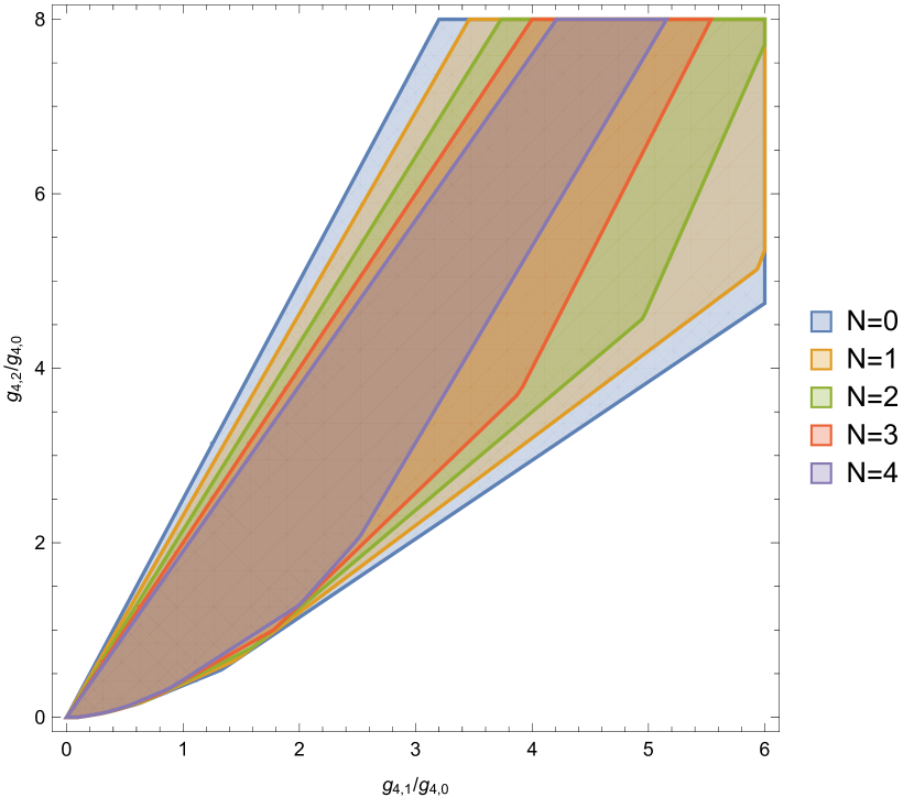
The region become smaller is reflected the fact, the decomposition of $\mathcal{N}$ super polynomial is positive sum of $\mathcal{N}{-}1$ polynomials. It can be easily show from recurrence relation

$$\begin{split}\frac{\partial}{\partial\eta^{A}_{2}}\frac{\partial}{\partial\eta^{A}_{4}}\mathcal{P}^{\mathcal{N}}_{\{H_{i}\},S}|_{\eta^{A}=0}=m^{2}\mathcal{P}^{\mathcal{N}-1}_{\{h_{i}\},S+\frac{1}{2}}+\frac{m^{2}(S-H_{3}+H_{4})(S-H_{1}+H_{2})}{\left(2S\right)\left(2S+1\right)}\mathcal{P}^{\mathcal{N}-1}_{\{h_{i}\},S-\frac{1}{2}}\,.\end{split}$$ (5.10)

RHS have positive coefficients when we identify $H_{1}=H_{3},H_{2}=H_{4}$ which means $\mathcal{N}$ super polynomial is living inside of $\mathcal{N}{-}1$ convex hull. As we know the boundary of $\mathcal{N}$ convex hull are living inside of $\mathcal{N}{-}1$, the $\mathcal{N}$ space must smaller than $\mathcal{N}{-}1$.

6 Conclusion

In this paper, we proposed an super Poincare invariant expansion basis for the residue and discontinuity of four-point amplitudes in four dimensions. These super spinning polynomials are given in terms of algebraic Jacobi functions, whose recurrence relations reflect the decomposition of the SUSY multiplet in terms of components. These polynomials were identified through gluing of three-point super amplitudes constructed out of massive and massless on-shell super space.

As an application, we use dispersion relations to derive bounds on EFT coefficients. By expanding the imaginary part of the amplitude on these super spinning polynomials, we derive bounds that reflect the underlying supersymmetric UV completion.

7 Acknowledgements

We would like to thank Yu-tin Huang for enlightening discussions. J-Y Liu and Z-M You are supported by MoST Grant No. 106-2628-M-002-012-MY3.

Appendix A Conventions

The convention we used in the central of mass frame. Spinor brackets are related to center of mass $m$ and scattering angle $\theta$:

$$\begin{split}&|1\rangle=m^{\frac{1}{2}}\left(\begin{array}[]{cc}1&\\ 0&\end{array}\right)\,,\quad|2\rangle=m^{\frac{1}{2}}\left(\begin{array}[]{cc}0&\\ 1&\end{array}\right)\\ &|3\rangle=im^{\frac{1}{2}}\left(\begin{array}[]{cc}sin\frac{\theta}{2}&\\ -cos\frac{\theta}{2}&\end{array}\right)\,,\quad|4\rangle=im^{\frac{1}{2}}\left(\begin{array}[]{cc}cos\frac{\theta}{2}&\\ sin\frac{\theta}{2}&\end{array}\right).\end{split}$$ (A.1)

Levi-Civita tensor is

$$\epsilon^{a\dot{a}}=\left(\begin{array}[]{cc}0&1\\ -1&0\end{array}\right).$$ (A.2)

Contraction of spinor brackets:

$\displaystyle\langle 12\rangle=m,\quad$ $\displaystyle\langle 34\rangle=-m$ (A.3)
โŸจ13โŸฉ=โˆ’iโ€‹mโ€‹cโ€‹oโ€‹sโ€‹(ฮธ2),delimited-โŸจโŸฉ13๐‘–๐‘š๐‘๐‘œ๐‘ ๐œƒ2\displaystyle\langle 13\rangle=-imcos(\frac{\theta}{2}),\quad โŸจ24โŸฉ=โˆ’iโ€‹mโ€‹cโ€‹oโ€‹sโ€‹(ฮธ2)delimited-โŸจโŸฉ24๐‘–๐‘š๐‘๐‘œ๐‘ ๐œƒ2\displaystyle\langle 24\rangle=-imcos(\frac{\theta}{2})
โŸจ14โŸฉ=iโ€‹mโ€‹sโ€‹iโ€‹nโ€‹(ฮธ2),delimited-โŸจโŸฉ14๐‘–๐‘š๐‘ ๐‘–๐‘›๐œƒ2\displaystyle\langle 14\rangle=imsin(\frac{\theta}{2}),\quad โŸจ23โŸฉ=โˆ’iโ€‹mโ€‹sโ€‹iโ€‹nโ€‹(ฮธ2).delimited-โŸจโŸฉ23๐‘–๐‘š๐‘ ๐‘–๐‘›๐œƒ2\displaystyle\langle 23\rangle=-imsin(\frac{\theta}{2}).

The Mandelsteine variables define as

s=โˆ’(P1+P2)2,t=โˆ’(P1+P4)2,u=โˆ’(P1+P3)2formulae-sequence๐‘ superscriptsubscript๐‘ƒ1subscript๐‘ƒ22formulae-sequence๐‘กsuperscriptsubscript๐‘ƒ1subscript๐‘ƒ42๐‘ขsuperscriptsubscript๐‘ƒ1subscript๐‘ƒ32\displaystyle s=-(P_{1}+P_{2})^{2},\quad t=-(P_{1}+P_{4})^{2},\quad u=-(P_{1}+P_{3})^{2}
โ‡’s=m2,t=โˆ’m2โ€‹(1โˆ’cโ€‹oโ€‹sโ€‹ฮธ)2,u=โˆ’m2โ€‹(1+cโ€‹oโ€‹sโ€‹ฮธ)2.formulae-sequenceโ‡’absent๐‘ superscript๐‘š2formulae-sequence๐‘กsuperscript๐‘š21๐‘๐‘œ๐‘ ๐œƒ2๐‘ขsuperscript๐‘š21๐‘๐‘œ๐‘ ๐œƒ2\displaystyle\Rightarrow s=m^{2},\quad t=-m^{2}\frac{(1-cos\theta)}{2},\quad u=-m^{2}\frac{(1+cos\theta)}{2}. (A.4)

References

  • (1) H. Elvang and Y. Huang, Scattering Amplitudes in Gauge Theory and Gravity. Cambridge University Press, 2015, arXiv:1308.1697
  • (2) C. Cheung, TASI Lectures on Scattering Amplitudes, arXiv:1708.03872 [hep-ph].
  • (3) N. Arkani-Hamed, T.-C. Huang and Y.-t. Huang, Scattering Amplitudes For All Masses and Spins, arXiv:1709.04891.
  • (4) A. Herderschee, S. Koren, and T. Trott, Massive On-Shell Supersymmetric Scattering Amplitudes, arXiv:1902.07204.
  • (5) Caron-Huot, S., Zahraee, Z. Integrability of black hole orbits in maximal supergravity. J. High Energ. Phys. 2019, 179 (2019). https://doi.org/10.1007/JHEP07(2019)179
  • (6) Herderschee, A., Koren, S. and Trott, T. Constructing N = 4 Coulomb branch superamplitudes. J. High Energ. Phys. 2019, 107 (2019). https://doi.org/10.1007/JHEP08(2019)107
  • (7) N.ย Arkani-Hamed, T-z Huang and Y-t.ย Huang, in preparation.
  • (8) N. Arkani-Hamed, F. Cachazo, and J. Kaplan, What is the Simplest Quantum Field Theory?, JHEP 09 (2010) 016, [arXiv:0808.1446].