Low luminosity Type II supernovae – III. SN 2018hwm, a faint event with an unusually long plateau

Abstract

In this work, we present photometric and spectroscopic data of the low-luminosity Type IIP supernova (SN) 2018hwm. The object shows a faint ($M_{r}=-15$ mag) and very long ($\sim$130 days) plateau, followed by a 2.7 mag drop in the $r$-band to the radioactive tail. The first spectrum shows a blue continuum with narrow Balmer lines, while during the plateau the spectra show numerous metal lines, all with strong and narrow P-Cygni profiles. The expansion velocities are low, in the 1000-1400 km s^-1 range. The nebular spectrum, dominated by H$\alpha$ in emission, reveals weak emission from [O I] and [Ca II] doublets. The absolute light curve and spectra at different phases are similar to those of low-luminosity SNe IIP. We estimate that 0.0085 $M_{\odot}$ of ⁵⁶Ni mass were ejected, through hydrodynamical simulations. The best fit of the model to the observed data is found for an extremely low explosion energy of 0.075 foe, a progenitor radius of 845 $R_{\odot}$ and a final progenitor mass of 9-10 $M_{\odot}$. Finally, we performed a modeling of the nebular spectrum, to establish the amount of oxygen and calcium ejected. We found a low M(¹⁶O)$\approx 0.02$ $M_{\odot}$, but a high M(⁴⁰Ca) of 0.3 $M_{\odot}$. The inferred low explosion energy, the low ejected ⁵⁶Ni mass and the progenitor parameters, along with peculiar features observed in the nebular spectrum, are consistent with both an electron-capture SN explosion of a super-asymptotic giant branch star and with a low-energy, Ni-poor iron core-collapse SN from a 10-12 $M_{\odot}$ red supergiant.

1 Introduction

Type II supernovae (SNe) are luminous events that originate from the explosion of a massive ($>8M_{\odot}$) star. Historically, Type II SNe were subdivided in two main subclasses (Barbon, Ciatti & Rosino, 1979) based on their photometric behaviour, namely Type IIL (with a linearly declining light curve after maximum) and Type IIP SNe. The latter represent events whose luminosity stays at a nearly constant luminosity for a long period, hence called ‘plateau’ phase. The long plateau of SNe IIP (90-100 days, Hamuy et al., 2003) is due to the energy released by the hydrogen envelope as it cools and recombines, after being fully ionized by the explosion. Much work has been done to characterize the properties of SNe IIP through the analysis of large samples of objects (Li et al., 2011; Arcavi et al., 2012; Anderson et al., 2014; Faran et al., 2014a; Gutiérrez et al., 2014; Sanders et al., 2015; Valenti et al., 2016; Gutiérrez et al., 2017a, b). In particular, a small group of SNe IIP are remarkably less luminous than average. The first sub-luminous SN IIP discovered was SN 1997D (Turatto et al., 1998; Benetti et al., 2001), that had a peak luminosity of only $M_{B}=-14.65$ mag. During the nebular phase, the light curve of SN 1997D shows a tail with a declining slope compatible with the radioactive decay of ⁵⁶Co, indicating that at this late time the luminosity of the object is solely powered by a small amount of radioactive material (2$\times 10^{-3}$ $M_{\odot}$).

SN 1999br (Zampieri et al., 2003; Pastorello et al., 2004) was very similar in luminosity and spectral appearance to SN 1997D, with narrow metal lines indicating low expansion velocities and unusually strong Ba II lines. In addition, SN 1999br showed a long plateau, lasting at least 110 days. A long plateau is indicative of a large recombination time, and may constitute evidence for the presence of a massive H envelope, that is consistent with the deduced massive ejecta (14 $M_{\odot}$, Zampieri et al., 2003).

SN 2003Z (Knop et al., 2007; Utrobin, Chugai & Pastorello, 2007; Spiro et al., 2014) was spectroscopically well followed among low-luminosity (LL) SNe IIP, with spectra that cover all evolutionary phases, from the early plateau, showing broad P-Cygni features, to the nebular phase.

The LL SN IIP SN 2005cs (Pastorello et al., 2006, 2009) exploded in the nearby (8.4 Mpc) galaxy M 51. Because of the small distance, it was possible to directly observe the progenitor star in archive Hubble Space Telescope ($HST$) images, that appeared to be a Red Supergiant (RSG) with an initial mass in the 7–13 $M_{\odot}$ range (Maund, Smartt & Danziger, 2005; Li et al., 2006; Takàts & Vinkò, 2006). The proximity of SN 2005cs also allowed observations of its faint radioactive tail, and it was obtained an ejected ⁵⁶Ni mass of only 3$\times 10^{-3}$ $M_{\odot}$ (Pastorello et al., 2009).

Gal-Yam et al. (2011) conducted a multi-wavelength follow-up of the LL SN 2010id, from $\gamma$-rays to the radio. It was observed extremely early, with a spectrum taken only 1.5 days after explosion. The rise to the plateau phase lasted less than 2 days.

Another remarkable object was SN 2016bkv (Nakaoka et al., 2018), which showed a very long plateau of 140 days, and an early bump in the light curve. A similar bump was likely observed also in SN 2003Z (Spiro et al., 2014). During the bump, the spectrum showed a blue continuum and a narrow H$\alpha$ emission, resembling those observed in Type IIn SNe, that indicate interaction between the SN ejecta and pre-existing circumstellar material (CSM). The presence of CSM suggests that the progenitor experienced mass loss just before the explosion.

The family of LL SNe IIP has been extended by the samples of Pastorello et al. (2004) and Spiro et al. (2014), and all objects share similar properties: low-luminosity, with absolute magnitudes $M_{V}$ during the plateau between $\sim-14$ and $\sim-15.5$ mag, compared to the average absolute magnitude of normal IIP SNe of $-16.7$ mag (Anderson et al., 2014), narrow spectral lines indicating low expansion velocities of about 1000 km s^-1, and small ejected ⁵⁶Ni masses ($<10^{-2}M_{\odot}$), one order of magnitude smaller than normal SNe (Benetti et al., 2001; Spiro & Pastorello, 2009). Another remarkable property of LL SNe IIP is the presence of narrow-lined spectra during the plateau, although narrow spectral lines were seen also in transitional IIP objects.

The luminosity gap between normal and faint SNe IIP has been filled in fact by a few ‘transitional’ objects including: SNe 2008in (Roy et al., 2011), 2009N (Takàts et al., 2014), 2009js (Gandhi et al., 2013), 2013am (Zhang et al., 2014; Tomasella et al., 2018), 2013K (Tomasella et al., 2018) and 2018aoq (O’Neill et al., 2019). These objects create a continuous distribution of luminosity among Type IIP SNe. Whilst transitional SNe IIP are brighter than faint ones, the low expansion velocities inferred from the spectral lines resemble those observed in LL SNe IIP.

An extended survey conducted on pre-explosion images of normal Type IIP SNe have confirmed that Red Super-Giant (RSG) stars, with masses in the range 8-16 $M_{\odot}$, are the most plausible progenitors of those objects (Smartt et al. 2009 and references therein, Van Dyk 2012, Maund et al. 2014a, Smartt 2015). A low mass, RSG star of 8-8.5 $M_{\odot}$, with a radius of 500 $R_{\odot}$, was identified as the progenitor of SN 2008bk (Mattila et al. 2008, Van Dyk et al. 2012, Maund et al. 2014b, Pignata et al., in preparation), and of SN 2003gd (8-9 $M_{\odot}$, Van Dyk, Li & Filippenko 2003, Smartt et al. 2004). Evolutionary numerical simulations of a Main Sequence (MS) 12 $M_{\odot}$ star reproduce the observed features of SN 2008bk, confirming a low-mass supergiant as the progenitor (Lisakov et al., 2017). Fraser et al. (2011) calculate the most probable progenitor mass range for the subluminous Type IIP SNe to be between 7.5 and 9.5 $M_{\odot}$, hence LL SNe IIP could arise from the lower-mass-end of RSG or Super-Asymptotic Giant Branch (SAGB) stars.

The properties of the progenitors of SNe, such as mass and radius, can be derived also by modelling light curves and spectra, and through hydrodynamical simulations (Chugai & Utrobin, 2000; Utrobin, Chugai & Pastorello, 2007; Utrobin & Chugai, 2008; Bersten et al., 2011; Morozova et al., 2016). The simulations indicate that some LL SNe IIP come from low-to-moderate mass and large radii progenitors (250-500 $R_{\odot}$, 10-11 $M_{\odot}$ ejecta, 13-15 $M_{\odot}$ on MS), with low explosion energies ($\sim$10⁵⁰ erg, Pumo et al., 2017).

More recently, another promising way to derive physical characteristics of the progenitor has been proposed by modeling nebular spectra (e.g. Jerkstrand et al. 2012, 2014, 2018). The presence/absence and the strength of some specific lines, such as the [O I] and [Ca II] doublets, give important clues on the initial mass and progenitor’s type.

In this context, in this paper we present a study of SN 2018hwm, a new LL SN IIP exploded in the relatively nearby galaxy IC 2327, and with a very long plateau. The paper is structured as follows: In Sect. 2 the discovery of SN 2018hwm and the properties of its host galaxy are reported. In Sect. 3 we present and analyse the photometric data. The spectra are presented in Sect. 4. In Sect. 5 we discuss the nature of the progenitor and the explosion scenario of SN2018hwm on the basis of the SN’s observables.

2 Discovery and host galaxy

SN 2018hwm (a.k.a. ZTF18acurqaw, ATLAS18zrw, PS18byn) was discovered by the Puckett Observatory Supernova Search (POSS; Gagliano et al., 2018), on 2018 November 4.51 (UT) in the galaxy IC 2327 (or UGC 4356), at celestial coordinates $\alpha$ = 08:21:28.192, $\delta$ = +03:09:52.35 (J2000). At discovery, the unfiltered magnitude of the transient was 19.2. A colour image of the host galaxy with the SN taken 4 months after the discovery, and obtained combining the frames in the $g$, $r$ and $i$ filters, is shown in Figure 1.

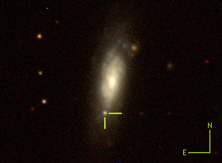
Figure 1: Colour image of the host galaxy IC 2327 and of SN 2018hwm taken on 2019 February 26, 4 months after explosion, with the Liverpool Telescope (Steele et al., 2004). The image is a combination of the frames obtained with the $g$, $r$ and $i$ filters. The location of the SN is marked.

The spectroscopic classification of SN 2018hwm was performed 4 days after discovery by the extended Public ESO Spectroscopic Survey for Transient Objects (ePESSTO; Smartt et al., 2015) collaboration with the ESO 3.58-m New Technology Telescope (NTT). The transient was classified as a young type II SN, showing a blue continuum and P-Cygni Balmer lines (Congiu et al., 2018). The tools used for the classification were GELATO (Harutyunyan et al., 2008) and SNID (Blondin & Tonry, 2007). The classification spectrum is presented in Sect. 4. Later, the transient developed the typical features of SNe IIP (see Sect. 4).

IC 2327 is an Sa spiral galaxy according to De Vaucouleurs (1991). The NASA/IPAC Extragalactic Database (NED) reports different measurements of distance of IC 2327, all obtained through the Tully-Fisher relation method (e.g. Tully et al., 2016). We adopt the weighted mean value of $52\pm 5$ Mpc, assuming a standard cosmology ($H_{0}=73$ km s^-1Mpc^-1, $\Omega_{m}=0.27$, $\Omega_{\Lambda}=0.73$). This translates in a distance modulus (DM) of 33.58$\pm$0.19 mag. The redshift of the host galaxy $z=0.00895\pm 0.00002$ is from Falco et al. (1999). The Milky Way reddening in the direction of IC 2327 is $A_{V,MW}=0.071$ mag (Schlafly et al., 2011). The extinction contribution of the host galaxy is negligible, as in the spectra (Sect. 4.1) we do not see absorption lines from the Na I D doublet at the host galaxy redshift, that would suggest the presence of additional dust.

In order to understand the nature of the progenitor of SN 2018hwm, we evaluated some properties of the host galaxy, including the metallicity and the star formation rate. We estimated the metallicity of the host galaxy through the correlation between the mean [O/H] metallicity indicator and the $B$-band absolute magnitude of the galaxy (Pilyugin, Vílchez & Contini, 2004). From the HyperLeda database, IC 2327 has $M_{B}=-19.93\pm 0.42$ mag. Using equation 12 from Pilyugin et al. 2004 for spiral galaxies, we obtain 12+log[O/H]_host=8.50$\pm 0.77$. Assuming a solar value of 12+log[O/H]_⊙=8.69 (Asplund et al., 2009), this corresponds to $Z=0.013$ (adopting $Z_{\odot}=0.02$), thus we may conclude that the oxygen abundance of the host is nearly solar.

To estimate the star formation rate (SFR) in IC 2327, we use the Kennicutt (1998) relation between the SFR and the luminosity in the far ultraviolet (FUV) region: $SFR(FUV,M_{\odot}yr^{-1})=1.4\times 10^{-28}L(FUV,erg\cdot s^{-1}Hz^{-1})$. The NED database reports two integrated flux densities in the FUV (at 1530 Å) from GALEX, of 1.11 and 1.15 mJy. Taking the average flux density of 1.13 mJy and the assumed distance of 52 Mpc, we obtain a SFR of 0.51 $M_{\odot}yr^{-1}$ for IC 2327.

3 Photometry

The photometric follow-up of SN 2018hwm was performed with a plethora of instruments and telescopes, available to our collaborations, whose characteristics are reported in Table 1. Optical observations were done with Johnson-Cousins $BVRI$ and Sloan $griz$ filters, and in the near infrared (NIR) with $JHKs$ filters, albeit only for a few epochs.

Table 1: Observational facilities and instrumentation used in the photometric follow-up of SN 2018hwm.

Telescope	Location	Instrument	Filters
NOT (2.56m)	La Palma	ALFOSC	$BVgriz$
NOT (2.56m)	La Palma	NOTCAM	$JHKs$
LT (2.0m)	La Palma	IO:O	$BVgriz$
NTT (3.58m)	La Silla	EFOSC	$V$
TRAPPIST (0.6m)	La Silla	Fairchild	$BVRI$
Oschin (1.22m)	Mt. Palomar	ZTF	$gr$
SMARTS (1.3m)	CTIO	ANDICAM	$BVRI$
PROMPT3 (0.6m)	CTIO	Apogee	$iz$
PROMPT5 (0.4m)	CTIO	Apogee	$griz$
Blanco (4.0m)	CTIO	DECAM	$gr$
GTC (10.4m)	La Palma	OSIRIS	$r$

For the photometric data reduction we used a dedicated pipeline called SNOoPy (Cappellaro, 2014). An exhaustive description of the reduction procedures can be found in Reguitti et al. (2019). The instrumental magnitudes are determined through the PSF-fit method. For Sloan filter images, the photometric zero points and colour terms were computed through a sequence of reference stars from the SDSS survey in the SN field. For Johnson $BV$ filter frames, magnitudes for those reference stars were taken from the APASS DR10 catalogue. Finally, for NIR images, the magnitudes were calibrated with the 2MASS catalogue (Skrutskie et al., 2006). Photometric errors were estimated through artificial star experiments, also accounting for uncertainties in the PSF-fitting procedure and the colour terms.

The observed optical Sloan, Johnson and NIR magnitudes are listed in Table A1, A2 and A3, respectively.

3.1 Light curve evolution

The light curves of SN 2018hwm are plotted in Figure 2. The $r$-band light curve is the best sampled, and it is used as a reference for studying the photometric evolution of SN 2018hwm. The Zwicky Transient Facility (ZTF; Bellm et al. 2019, Graham et al., 2019) survey reports the last non-detection (at 20.9 mag) on 2018 November 1 (MJD 58423.5), while the first detection of the transient is reported 3 days later, on MJD 58426.5, nearly contemporary to the POSS discovery (Gagliano et al., 2018). Because of this, we adopt MJD 58425.0$\pm$1.5 as the most likely explosion epoch. The maximum light is reached about 5.5 days after explosion. The maximum is followed by the plateau phase, which ends at +130 d from explosion, comparable to that of SN 2009ib (Takàts et al., 2015), which is longer than for normal SNe IIP, whose plateau generally lasts 90-100 days (Hamuy et al., 2003). During the plateau, the magnitude of the object remains nearly constant at $r=18.5\pm 0.1$ mag. The post-plateau decline lasts around 1 month, and finally the SN sets into the radioactive slope at $r=21.2\pm 0.2$ mag, resulting in a drop of $\sim$2.7 mag, which is quite common in SNe IIP, see Olivares et al. (2010). A similar drop of about 2.5 mag is observed also in the $V$ light curve. Then, the SN went into solar conjunction, and when visible again, was recovered at 22.2$\pm$0.1 mag (phase +335 d).

In the $g$-band, after the maximum, the light curve declines with a rate of $2.6\pm 0.2$ mag (100 d)^-1 for about 40 days before reaching the plateau, that lasts until +120 d. In the other bands, the plateau and the following drop are only partially covered. The $B$-band follow-up started only 2 months after maximum; between +60 and +115 d the light curve in the $B$ filter does not show a plateau, but a linear decline with a slope of $0.96\pm 0.02$ mag (100 d)^-1.

Two additional photometric data points were collected in the $r$-band, about one year after explosion. Between +170 d and +390 d the observed decline slope is $0.74\pm 0.06$ mag (100 d)^-1, slower than the rate expected from the ⁵⁶Co radioactive decay (0.98 mag (100 d)^-1). Such a flattening during the early nebular phase has been previously observed by Pastorello et al. (2004) in SN 1999eu. However, we note that between the 2 final detections, the decline rate is $1.1\pm 0.3$ mag (100 d)^-1, consistent with the value of the ⁵⁶Co decay.

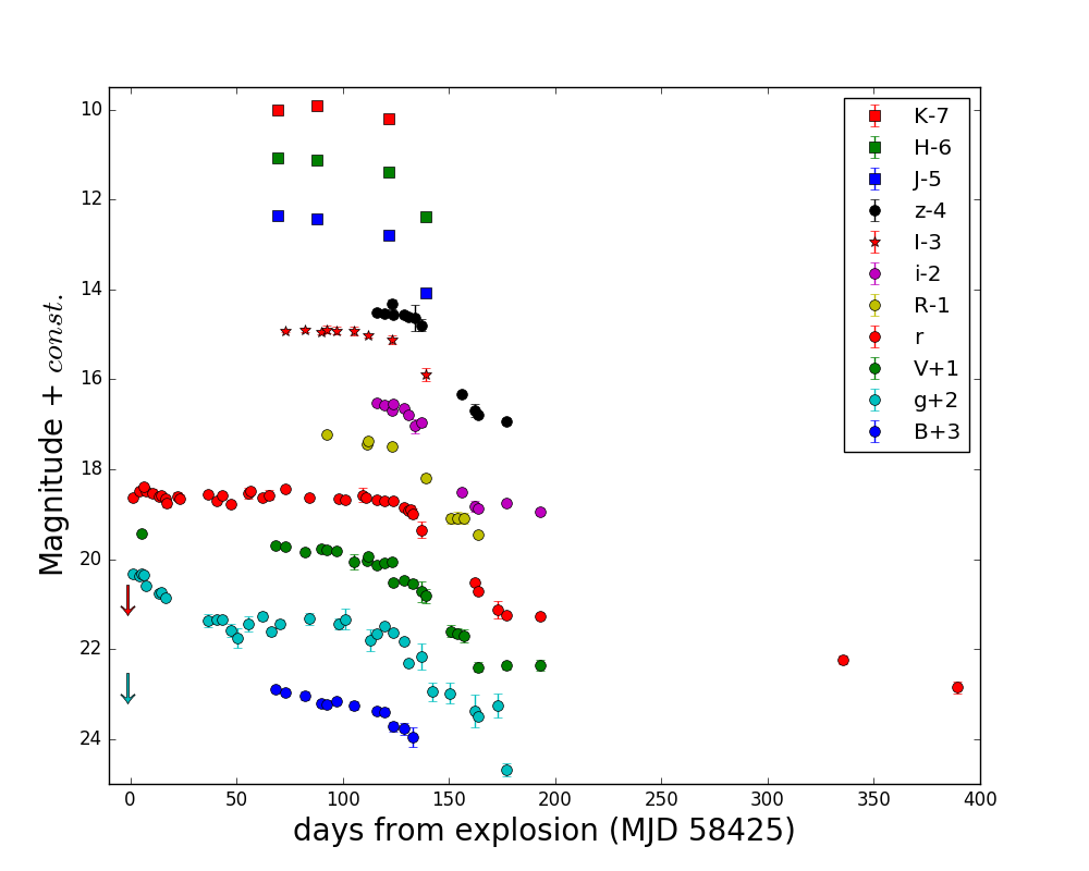
Figure 2: Multiband ($BVRIgrizJHK$) light curves of SN 2018hwm, covering 400 days of evolution. The phases are relative to the assumed explosion epoch (MJD 58425.0$\pm$1.5). For clarity the curves of different filters are shifted by a constant.

The duration of the plateau of SN 2018hwn ($\sim$130 d) is unusually long with respect that that observed in normal Type IIP SNe. Anderson et al. (2014) conducted a study of 116 SNe IIP, and found that the distribution of the optically thick phase duration (OPTd), i.e. the time between the explosion and the end of the plateau, has a mean value of 84 days, with a dispersion of 17 days. The largest OPTd in their sample is observed for SN 2004er, with a duration of 120 d. Larger OPTds are also derived for the sub-luminous events (see also Valenti et al. 2016). Arcavi et al. (2012) and Faran et al. (2014a) found that the peak of the plateau duration distribution is around 90-100 days. If one considers the time between the explosion and the mid point of the transition from the ‘plateau’ to the radioactive tail ($t_{PT}$ in Anderson et al. 2014), for SN 2018hwm this is 150 days, while Sanders et al. (2015) for normal SNe IIP found values in the range 60-140 days, with a median at around 110 days. Again, the longest $t_{PT}$ is observed for SN 2004er, and is similar to that of SN 2018hwm.

3.2 Absolute light curve

We constructed the absolute $r$-band light curve of SN 2018hwm, adopting the Galactic reddening and DM from Sect. 2. With these assumptions, the average absolute magnitude of SN 2018hwm during the plateau is $M_{r}=-15.0\pm 0.2$ mag. During the plateau the object was fainter in $g$-band, with the absolute magnitude staying constant at -14 mag between +40 and +120 days. After the end of the plateau, the $r$ absolute magnitude of SN 2018hwm dropped to -12.5 mag. A similar value is reached also in the other bands (-12.2 in $g$, -12.3 in $V$), whereas in redder filters it remains a bit more luminous (-13.0 in $i$, -13.2 in $z$). During the radioactive tail the object further weakened, with last detection (+389 d) being at an absolute magnitude $M_{r}=-10.8\pm 0.2$.

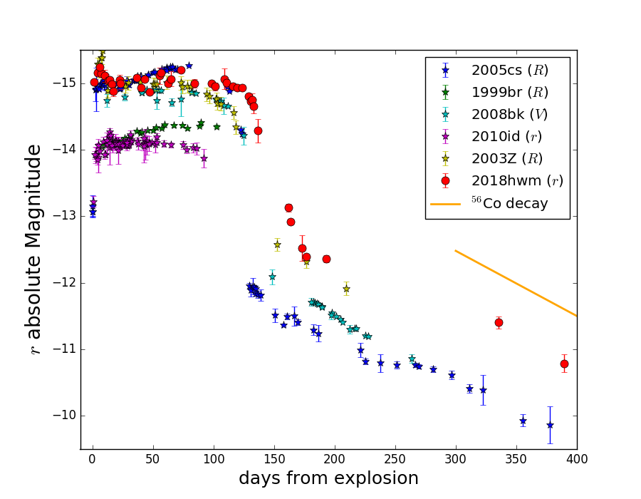
Figure 3: $r$-band absolute light curve of SN 2018hwm compared to absolute light curves of LL IIP objects: SNe 1999br (Pastorello et al. 2004), 2005cs (Pastorello et al. 2009), 2008bk (Van Dyk et al. 2012), 2003Z (Spiro et al. 2014) and 2010id (Gal-Yam et al. 2011). Distance moduli and reddenings of the comparison objects are taken from their respective papers. The expected decay slope of ⁵⁶Co (0.98 mag (100 d)^-1) is plotted for comparison.

We compared the absolute $r$-band light curve of SN 2018hwm with those of other known faint Type IIP SNe, i.e. SNe 1999br (Pastorello et al., 2004), 2005cs (Pastorello et al., 2009), 2008bk (Van Dyk et al., 2012), 2003Z (Spiro et al., 2014) and the particularly faint 2010id (Gal-Yam et al., 2011). The distance modulus and reddening of each object are taken from the respective papers, and are rescaled to $H_{0}=73$ km s^-1Mpc^-1. As can be seen in Figure 3, the light curve of SN 2018hwm is similar in luminosity to those of SNe 2005cs, 2003Z and 2008bk, both at peak and during the plateau. However, the plateau phase in SN 2018hwm lasts nearly one month more than in other faint Type IIP SNe. The drop from the plateau begins around +130 days after explosion. In addition, the drop from the plateau in SN 2018hwm is smaller: SN 2018hwm is $\sim 1$ mag brighter than SNe 2005cs and 2008bk during the nebular phase (between 6 and 12 months after explosion).

In the context of large samples of SNe IIP, LL IIP are placed on the faint tail of a continuous distribution in luminosity. The sample of Anderson et al. (2014) is characterized by a mean absolute magnitude at peak of $M_{V,max}=-16.7$ mag, with a scatter of 1 mag. Differently, Li et al. (2011) obtained an even fainter average absolute magnitude of $-16.1$ mag for a sample of Type II SNe, because of a different selection criteria of the sample. While SN 2018hwm, with a maximum $M_{r}$ of -15.2 mag (see Figure 3), can be considered a faint object with respect to the global population of SNe IIP, it is a relatively luminous event in the context of the faint SNe IIP subgroup (Pastorello et al., 2004; Spiro et al., 2014).

4 Spectroscopy

The spectroscopic monitoring of SN 2018hwm lasted about 1 year, during which we collected 6 optical spectra (see Table 2). All the spectra will be publicly released on the WISeREP repository (Yaron & Gal-Yam, 2012).

Table 2: Log of the spectroscopic observations of SN 2018hwm. For each spectrum, the date, the observed spectral range, the resolution, the exposure time and the telescope+instrument used are listed. The reported phases are relative to the assumed explosion time (MJD 58425.0, see Sect. 3.1).

Date	MJD	Phase	Coverage	Resolut.	Exposure	Telescope +
		(d)	(Å)	(Å)	(s)	Instrument
2018/11/08	58430.33	+5.3	3640-9230	18	600	NTT+EFOSC2
2018/12/17	58468.44	+43.4	3950-9220	25	2250	P200+SEDM
2019/01/08	58491.04	+66.0	3620-9640	19	2400	NOT+ALFOSC
2019/01/15	58498.02	+73.0	3740-9640	18	2500	NOT+ALFOSC
2019/02/21	58535.97	+111.0	3850-9640	18	2700	NOT+ALFOSC
2019/10/27	58814.20	+389.2	5100-10400	6	1380	GTC+OSIRIS

The NTT classification spectrum, taken through the ePESSTO program, was reduced with a pyraf-based pipeline (PESSTO, Smartt et al., 2015), optimised for the EFOSC2 instrument. The reduction operations performed by the pipeline include standard procedures: correction for bias and flat-field, extraction of the 1-D spectrum, removal of sky lines and cosmic rays, wavelength and flux calibrations, using arc lamps and spectrophotometric standard stars.

The ZTF survey collected one low-resolution spectrum with the 200-inch Mount Palomar telescope and the SED Machine spectrograph (SEDM; Blagorodnova et al., 2018), that was reduced using the pysedm (Rigault et al., 2019) automatic pipeline. The spectra from the NOT telescope were reduced using the ALFOSCGUI pipeline (Cappellaro, 2014), designed specifically for quickly reducing photometric and spectroscopic images taken with the ALFOSC instrument, as part of the NOT Unbiased Transients Survey (NUTS) collaboration (Mattila et al., 2016). The nebular spectrum from GTC was reduced with routine IRAF procedures.

The final spectra are corrected for the strongest telluric absorption bands, for redshift and for Galactic reddening using the Cardelli, Clayton & Mathis (1989) extinction law, and calibrated to match the closest broad-band photometry. The six spectra and the identified lines are shown in Figure 4.

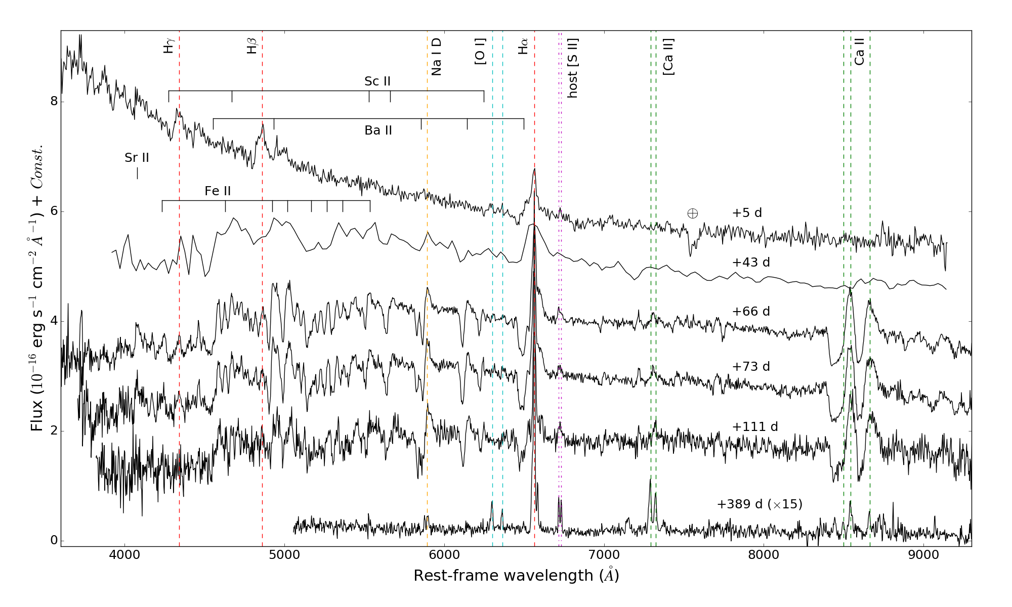
Figure 4: The six spectra of SN 2018hwm, redshift- and reddening-corrected. The spectra are shifted in flux by a constant for clarity. The principal identified lines are marked. Heavy elements transitions are marked by short vertical lines, grouped by element. The strong telluric absorption band, not fully corrected in the ePESSTO spectrum, is also marked. The [S II] lines are marked differently, as they are interpreted as host galaxy contamination.

4.1 Spectral evolution and line identification

The first spectrum, taken at around the maximum light, shows a blue continuum (with a black body temperature of 12000 K), and Balmer lines that have a relatively broad P-Cygni component, with a minimum blue-shifted by 4500 km/s, and a more prominent emission component, with $v_{FWHM}\sim$4000 km/s. Prominent, unresolved narrow emission lines from [O III] and [S II], superimposed to the broad components, are due to host galaxy contaminating sources (Congiu et al., 2018).

We used the tools SNID (Blondin & Tonry, 2007) and GELATO (Harutyunyan et al., 2008) to spectroscopically establish the explosion epoch, based on a comparison between the first spectrum of SN 2018hwm and early spectra of other Type IIP SNe, with well-determined explosion time estimation, and searching for the most similar spectra. The software found a good match with the spectra of SN 2005cs taken between 4 and 8 days after the explosion, consistent with our assumption about the explosion epoch of SN 2018hwm.

Although the second spectrum is of a lower quality than the first, absorption features from once ionized metal elements (including Fe II, Ba II and Sc II, see the identification of Pastorello et al., 2004) start to emerge from a colder continuum ($T_{bb}\sim$ 6900 K).

We collected three spectra during the plateau phase, that show the typical features of Type IIP SNe. The three spectra, taken between 2 and 4 months after explosion, do not show a significant evolution, apart from a slow and modest decrease of the continuum temperature, with $T_{bb}$ decreasing from 4800 to 4500 K. Together with H$\alpha$ and H$\beta$, we identify numerous lines coming from transitions of metals. All the lines present an evident and narrow P-Cygni absorption. We measure the expansion velocity of the ejecta from the position of the minimum of the P-Cygni component in the three NOT spectra, and the values are reported in Table 3.

In the first photospheric spectrum the average veocity is 1400 km s^-1, while it decreases to 1300 km s^-1 in the second, and to 1000 km s^-1 in the third spectrum. The low velocities are an indication of a low explosion energy. The metal absorption lines in the spectra of SN 2018hwm are very narrow, resembling those observed in transitional objects between normal and faint Type IIP SNe, like SNe 2013K and 2013am (Tomasella et al., 2013). In the NIR part of the late spectra, two strong lines from the Ca II NIR triplet are detected.

The expansion velocity of the ejecta are relatively low in SN 2018hwm at all phases in comparison with the typical values observed in SNe IIP. Gutiérrez et al. (2017a) studied a sample of 122 SNe IIP, to infer the observed parameters of this class of objects. The ejecta expansion velocities at phase +50 d, measured from the FWHM of the H$\alpha$ line, are distributed between 9600 and 1500 km s^-1, with a median value of 7300 km s^-1. Around +100 d the velocities have decreased, but are still found within the 3000 to 7000 km s^-1 range. There are some noticeable outliers in the general distribution: SNe 2009aj and 2009au show low velocities, but are brighter than faint SNe IIP, and are known as luminous low expansion velocities SNe (LLEV; Rodriguez et al. 2019). For SN 2018hwm we obtained a mean ejecta velocity of 1400 km s^-1 in the +66 d spectrum, and about 1000 km s^-1 at +111 d.

Table 3: Expansion velocities of the ejecta, measured from the position of the minimum of the P-Cygni profile of hydrogen and heavy metal lines, as observed in the three NOT spectra during the plateau phase. All velocities are in km s^-1. The typical error is of the order of $\pm 50$ km s^-1.

line	wavelength	spectrum 1	spectrum 2	spectrum 3
	(Å)	+66 d	+73 d	+111 d
Sr II	4078	-	1620	-
Fe II	4233	-	1630	1270
Sc II	4273	-	1050	-
Ba II	4554	-	1120	990
Fe II	4629	1420	1170	-
Sc II	4670	1540	1350	900
H$\beta$	4861	1480	1170	1110
Fe II	4924	1280	1280	730
Ba II	4934	-	-	790
Fe II	5018	1610	1610	900
Fe II	5169	1450	1570	-
Fe II	5267	1020	970	970
Fe II	5363	-	-	890
Sc II	5527	1360	1520	1030
Fe II	5535	1490	1460	970
Sc II	5663	1380	1270	-
Ba II	5854	1330	1380	970
Ba II	6142	1320	1370	1180
Sc II	6246	1340	1100	910
Ba II	6497	1250	-	1200
H$\alpha$	6563	1550	1370	1050

Finally, we secured a nebular spectrum of SN 2018hwm about 1 year after the explosion. At that time, the transient had an apparent magnitude $r\approx$22.8 mag, but thanks to the high sensitivity of the GTC+OSIRIS combination, the spectrum has good signal-to-noise ratio, and shows some interesting features. The spectrum is contaminated by the host galaxy contribution in the form of narrow (FWHM$\sim$7 Å) emission lines, that are narrower than the SN features (with a mean FWHM of 13 Å). Over a flat pseudo-continuum we identify SN emission lines of [O I] $\lambda\lambda$6300,6364, H$\alpha$, [Fe II] $\lambda$7155, [Ca II] $\lambda\lambda$7291,7323 and the 3 lines of the NIR Ca II triplet $\lambda\lambda\lambda$ 8498,8542,8662. A faint blend of He I $\lambda$5876 and Na I D $\lambda\lambda$5890,5896 are also present. We also identify contaminant emission lines from the host, like [N II] $\lambda$6584, H$\alpha$ and [S II] $\lambda\lambda$6716,6731. In particular, the H$\alpha$ line is made of 2 components: one from the SN, with a $v_{FWHM}$ of 600 km s^-1, and one stronger and narrower ($v_{FWHM}$=400 km s^-1, comparable to the spectral resolution of 300 km s^-1), from the host galaxy. The H$\alpha$ component from the SN is blue-shifted by 550 km s^-1, but a contribution from the host [N II] $\lambda$6548 line cannot be ruled out. The O I $\lambda$7774 line is not detected, whereas the O I $\lambda$8446 line is visible.

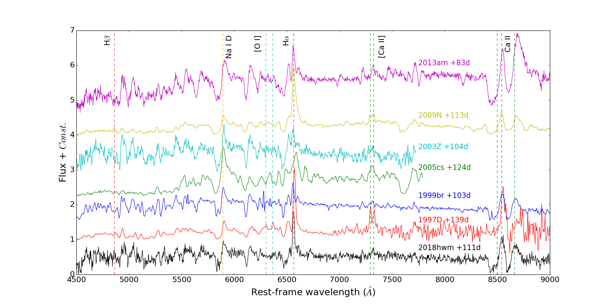
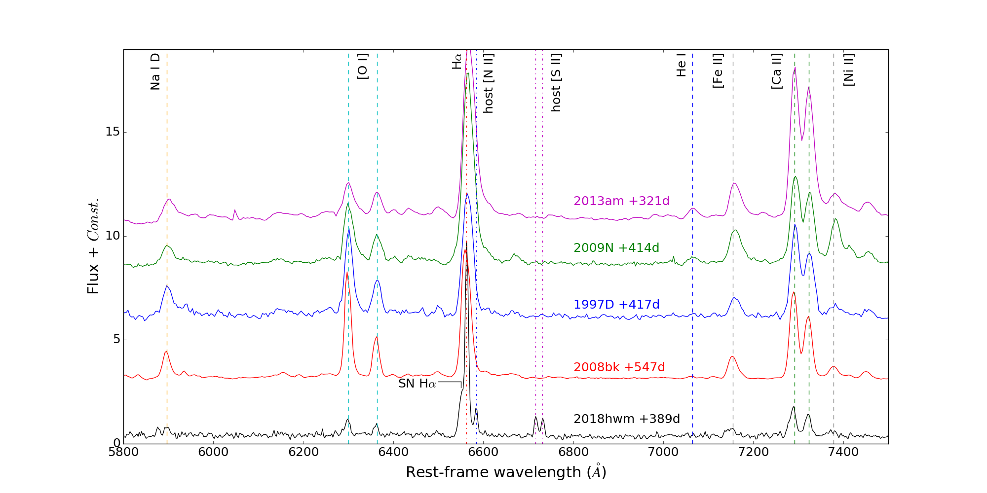
Figure 5: Top: The last photospheric spectrum of SN 2018hwm compared with the faint IIP SNe 1997D, 1999br, 2005cs, 2003Z and the transitionals SNe 2009N and 2013am at similar phases. Bottom: The nebular spectrum of SN 2018hwm is compared to those, taken at similar phases, of other faint IIP, SNe 1997D, 2008bk, 2009N and 2013am. Contaminant lines from the host are marked differently.

In Figure 5 (top) we compare the spectrum of SN 2018hwm taken at phase +113d, near to the end of the plateau, with those of both faint SNe IIP and transitional objects. The spectra of the comparison objects are taken close to the end of their plateaus. All these spectra are similar.

In Figure 5 (bottom), we compare the nebular spectrum of SN 2018hwm with those of two under-luminous objects, SNe 1997D and 2008bk (from Maguire et al., 2012), and two transitional objects, SNe 2009N and 2013am. The H$\alpha$ profile in SN 2018hwm is remarkable, showing a blue-shifted, broader component from the SN beside the narrower, host contribution. The higher spectral resolution of GTC+OSIRIS allows to better resolve the [Ca II] doublet. Indeed, the emission lines of SN 2018hwm are among the narrowest observed in the spectra of faint Type IIP SNe. Some differences in the spectrum of SN 2018hwm are noticeable: the Na I D, [O I] doublet, [Fe II] and also [Ca II] lines are fainter and narrower. Transitional objects show a weak He I 7065 emission, which is not detected in the spectra of fainter SNe.

5 Discussion

5.1 Bolometric light curve

We constructed the spectral energy distribution (SED) of SN 2018hwm from the available reddening-corrected photometry, spanning from $B$ to $K$ bands, and using the Sloan-$r$ as reference. When the photometric observation is missing in a given filter, its value is inferred from adjacent epoch photometry assuming a constant colour evolution. Then, we fitted the SED with a single black body curve, using the curve_fit tool of Python. The free parameters of the fit are the radius, the temperature and the bolometric luminosity of the black body, that is derived by integrating the black body curve over all wavelenghts, and assuming the distance modulus value reported in Section 2.1. The errors of the free parameters are estimated from the covariance matrix provided by curve_fit. The bolometric light curve and the evolution of the radius and temperature of the black body are plotted in Figure 6.

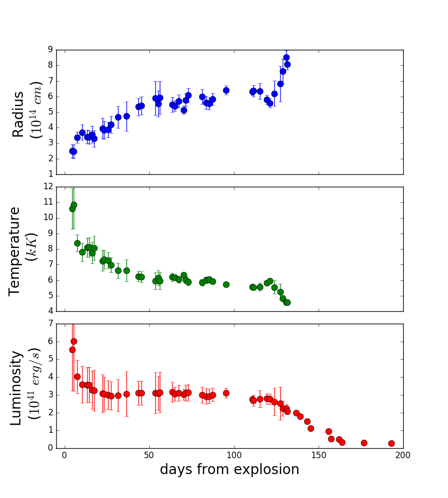
Figure 6: Top: evolution of the radius of the photosphere, obtained by fitting the SED with a single black body. Center: evolution of the temperature of the photosphere. The radius and temperature evolutions are plotted only until +130 d, then the black body fit becomes unreliable. Bottom: bolometric light curve, calculated from the Stefan-Boltzmann law $L=4\pi r^{2}\sigma T^{4}$. The phases are relative to the explosion epoch.

The fit of the SED with a black body after the plateau end is not reliable, as the spectrum becomes dominated by emission lines rather than the continuum. Thus, we considered the evolution of the radius and temperature only until +130 d. The black body radius starts to increase just after the explosion, levelling out to around 6$\times$10¹⁴ cm (8600 AU) during the plateau. At the end of the plateau, the radius sharply increases, reaching nearly 9$\times$10¹⁴ cm. The temperature of the black body drops rapidly after the explosion, from 11000 to 8000 K in a few days. Later on, the temperature slowly decrease from 7500 to 5000 K. The bolometric luminosity of SN 2018hwm shows an evolution similar to the one of the black body temperature, while also mirroring the $r$-band light curve. The mean bolometric luminosity during the plateau is 3$\times 10^{41}$ erg s^-1, and drops by a factor of 10 when the object enters in the nebular phase.

5.2 Hydrodynamical modelling

The physical properties of the progenitor of SN 2018hwm at the time of the explosion (the ejected mass $M_{ej}$, the progenitor radius at the explosion $R$ and the total explosion energy $E$) are derived using the same well-tested radiation-hydrodynamical modelling procedure that has been applied to other observed underluminous Type IIP SNe (e.g. Tomasella et al. 2013, Spiro et al. 2014, Takàts et al. 2014, Takàts et al. 2015, Pumo et al. 2017, Tomasella et al. 2018). A complete description of this procedure is found in Pumo et al. (2017). Here we recall its main features that can be summarized as follows.

• The SN progenitor’s physical properties at the time of the explosion are constrained through the hydrodynamical modelling of all the main SN observables (i.e. bolometric light curve, evolution of metal line velocities and the temperature at the photosphere), using a simultaneous $\chi^{2}$ fit of the observables against model calculations.

• The models are computed making use of the general-relativistic, radiation-hydrodynamics Lagrangian code presented in Pumo & Zampieri (2011). This code was specifically designed to simulate the evolution of the physical properties of SN ejecta and the behavior of the main SN observables during the entire post-explosive evolution (i.e. from the breakout of the shock wave at the stellar surface up to the radioactive-decay phase), taking into account both the gravitational effects of the compact remnant and the heating effects due to the decays of the radioactive isotopes synthesized during the explosion. The four basic parameters guiding the post-explosion evolution of these models are $M_{ej}$, $R$, $E$ and the ⁵⁶Ni mass, $M_{Ni}$, initially present in the ejecta of the models (see also Pumo & Zampieri, 2013).

• The free model parameters of the $\chi^{2}$ fit are $M_{ej}$, $R$ and $E$. $M_{Ni}$ is instead held fixed and its value is set so as to reproduce the observed bolometric luminosity during the radioactive decay phase.

• The observational data taken at the earliest phases (i.e. within the first $\sim$ 5 days after explosion for SN 2018hwm) are not included in the $\chi^{2}$ fit because the models could not accurately reproduce the early evolution of the main observables.

• A preparatory analysis, aimed at determining the parameter space describing the SN progenitor at explosion, is performed with the semi-analytic code described in Zampieri et al. (2003). This analysis guides the general-relativistic, radiation-hydrodynamics simulations that are more realistic but time consuming. Moreover the semi-analytic code is used to estimate the uncertainties on the free model parameters due to the $\chi^{2}$ fitting procedure. Possible systematic errors linked to the input physics (e.g. the opacity treatment) and to the assumptions made in evaluating the observational quantities (e.g. the adopted reddening or the adopted distance modulus) are not included.

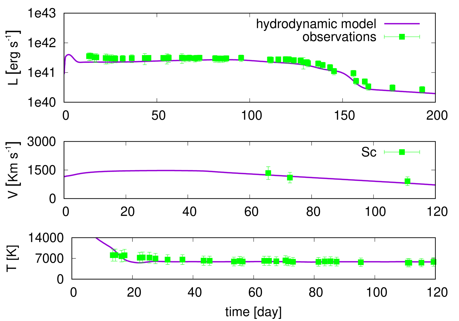
Figure 7: Comparison of the evolution of the main observables of SN 2018hwm with the best-fit model computed with the general-relativistic, radiation-hydrodynamics code. The best-fit model parameters are: total energy $0.075$ foe, radius at explosion $5.9\times 10^{13}$ cm, and ejected mass 8.0 $M_{\odot}$. Top, middle, and bottom panels show the bolometric light curve, the photospheric velocity, and the black-body photospheric temperature as a function of time, respectively. To better estimate the photosphere velocity from observations, we use the minimum of the profile of the Sc lines, as the Sc lines are generated just above the photosphere.

Based on the adopted explosion epoch (cfr. Sect. 3.1) and bolometric luminosity (cfr. Sect. 5.1), we find the best-fitting model shown in Figure 7. In particular, the inferred best-fit model has a kinetic plu thermal energy of 0.075 foe, radius at explosion of $5.9\times 10^{13}$ cm ($\sim$845 $R_{\odot}$), $M_{Ni}\simeq 0.0085$ and ejected mass of 8.0 $M_{\odot}$. Adding the mass of the compact remnant ($\sim$1.3-2 $M_{\odot}$) to that of the ejected material, we obtain a total stellar mass at explosion of $\sim$9.3-10.0 $M_{\odot}$. To estimate the initial mass of the progenitor on the MS, we assume a typical (i.e. not enhanced by rotation) mass loss during the pre-SN evolution $\lesssim$ 0.1-0.9 $M_{\odot}$ (see Pumo et al. 2017 and references therein for details). Hence, the initial progenitor mass is in the range 9.4-10.9 $M_{\odot}$. The estimated errors on the free model parameters due to the $\chi^{2}$ fitting procedure are about 15% for $M_{ej}$ and $R$, and 30% for $E$.

Popov (1993) and Kasen & Woosley (2009) derived scaling relations for the properties of SNe IIP, and concluded that the plateau duration is correlated to the envelope mass. While in SN 2018hwm the plateau is very long (nearly 140 days), the ejecta mass is not higher than the expectation from the analytical modelling of the explosion. The discrepancy is explained by the extremely low explosion energy (more than one order of magnitude smaller than the typical value derived by Kasen & Woosley (2009) ($\sim 0.9\times 10^{51}$ ergs). The low kinetic energy of the ejecta, and the consequent low expansion velocities, generate a slow-moning recombination. As a consequence, the plateau has a longer duration than that usually observed in SNe IIP. Pumo et al. (2017) noted that the main regulator of the distribution of IIP SNe properties (such as luminosity and ⁵⁶Ni mass) is in fact the ratio between the explosion energy and ejecta mass ($E/M_{ej}$). For SN 2018hwm, we evaluate the value of this ratio to $E/M_{ej}$=0.0094 foe/$M_{\odot}$, which is among the lowest calculated for a Type IIP SN (Pumo et al. 2017, Lisakov et al. 2018 and references therein), and is nearly half of what is derived for other low luminosity SNe IIP with known RSG progenitors.

5.3 Explosion and progenitor scenario

The derived explosion energy of SN 2018hwm (0.075 foe), when compared to the theoretical models (Sukhbold et al., 2016; Burrows et al., 2020; Limongi & Chieffi, 2020), is extremely low, even accounting for the error bar. Standard SN explosion simulations predict explosion energies above 0.2$\times 10^{51}$ erg, and up to 2$\times 10^{51}$ erg. Although it is difficult to explain such a low energy with a standard core-collapse SN, it is still possible. For example, SN 1054 (a.k.a. ‘the Crab event’) is believed to be the outcome of a ECSN (Kitaura, Janka & Hillebrandt, 2006) with an explosion energy of 0.1 foe (Sukhbold et al., 2016). In addition, using the scaling relations from Popov (1993), Müller et al. (2017) are able to obtain $E$ below 0.1 foe for a few normal Type II SNe.

The ⁵⁶Ni synthesized in SNe, which is the only source powering the late-time luminosity after the plateau stage, is largely formed by the explosive burning of oxygen and silicon. To explain the ejection of a small amount of ⁵⁶Ni in LL IIP, three main explosion scenarios have been formulated: (i) The fall-back of most of the material from the outer, Ni-rich region of a high mass (25-40 $M_{\odot}$) progenitor star onto its newly formed degenerate core (Woosley & Weaver 1995, Zampieri et al. 1998; Moriya et al. 2010). This phenomenon would naturally produce a low luminosity explosion event, and the apparent formation of small quantities of ⁵⁶Ni, as it falls back on to the newly born black hole. (ii) The detonation of a low mass (8–10 $M_{\odot}$) progenitor as a Fe core-collapse SN, in which very little ⁵⁶Ni is synthesized (Nomoto et al. 1982, Woosley & Weaver 1986, Chugai & Utrobin 2000). (iii) A third explosion scenario, that can explain the observed properties of faint IIP SNe (i.e. massive ejecta, low ⁵⁶Ni mass produced and low energetic events) is the explosion of a moderate-mass star, with O-Ne-Mg core, via Electron-Capture SN (ECSN; Nomoto 1984, Ritossa, García-Berro & Iben 1999, Heger et al. 2003, Kitaura, Janka & Hillebrandt 2006; Takahashi, Yoshida & Umeda 2013). The theory of stellar evolution predicts stars with a MS mass of 8 to 11 $M_{\odot}$ to become SAGB stars which may lead to ECSNe (e.g. Tominaga, Blinnikov & Nomoto, 2013). Kitaura, Janka & Hillebrandt (2006) and Eldridge, Mattila & Smartt (2007) noted that a SAGB progenitor will have little oxygen and silicon surrounding the core, and hence we may expect a SAGB star to produce a low mass of ejected ⁵⁶Ni.

Fransson & Chevalier (1989) suggested that the ratio $\Re$ between the luminosities of the [Ca II] $\lambda\lambda$7291,7324 and [O I] $\lambda\lambda$6300,6364 can be a good diagnostic for the main-sequence mass of the precursor star. We calculated this ratio for SN 2018hwm in the nebular spectrum (phase +389 d), and obtained $\Re\sim$2.7. A value of $\Re$ close to 3 is consistent with a low main-sequence progenitor mass, as estimated for SN 2005cs (7–13 $M_{\odot}$; Maund, Smartt & Danziger 2005, Li et al. 2006, Takàts & Vinkò 2006 and Eldridge, Mattila & Smartt, 2007).

The inferred values of the best-fit model parameters are consistent with an ECSN involving a SAGB star with initial mass close to the upper limit of the mass range typical of this class of stars (for further details see e.g. Pumo et al., 2009).

The best-fit model parameters may be also consistent with an iron core-collapse SN with a very low-energy explosion involving a low-mass red/yellow supergiant star. However, the inferred value of $E$ seems to be too low to consider this scenario as the most reliable, although it cannot be ruled out. Lacking information on the temperature and colour of the progenitor from pre-explosion images (as was obtained for SNe 2005cs and 2008bk), we cannot distinguish an SAGB from an RSG progenitor. The absence of signs of interaction with a pre-existing CSM, particularly in the spectra, has two possible explanations: (i) the progenitor experienced only very minor mass loss before the core-collapse, which is not expected from a star in the SAGB phase, or (ii) the progenitor was a SAGB that had recently ($\sim 10^{4}$ years, see Table 1 from Pumo et al. 2009) entered the Thermal Pulses phase. In the latter case, the star would have retained most of the envelope. This is ejected only in the final explosive event, such that a dense CSM is not present.

The progenitor mass of SN 2018hwm obtained from hydrodynamical simulations is in agreement with the value found for many subluminous SNe. For example, Spiro et al. (2014) propose a progenitor masses range of 10–15 $M_{\odot}$ for their sample of LL SNe IIP. Utrobin, Chugai & Pastorello (2007) modelled the light curves and spectra of SN 2003Z, obtaining a high ejecta mass of 14 $M_{\odot}$, that leads to an estimated initial mass of 16 $M_{\odot}$ but a small progenitor radius of 230 $R_{\odot}$. Pumo et al. (2017) found a similar value of 260 $R_{\odot}$. The small radius may favour a yellow supergiant as progenitor, instead of a red one, and it has been hypothesized for the transitional event SN 2009N (Takàts et al., 2014).

As mentioned before, we cannot provide conclusive arguments supporting one of the two explosion scenarios. As some observational properties seem to favour the ECSN and others the Fe-CC SN, we can here summarise their strong and weak arguments. The arguments in favour of an ECSN scenario for SN 2018hwm are:

• the low explosion energy ($7.5\times 10^{49}$ erg),

• the low synthesized ⁵⁶Ni mass (0.0085 $M_{\odot}$),

• the low initial progenitor mass (between 9 and 11 $M_{\odot}$),

• the absence of the He I $\lambda$7065 line (Jerkstrand et al., 2018).

On the other hand, the more canonical Fe-CCSN scenario can also explain some of the observed properties, such as:

• a star with a radius of 845 $R_{\odot}$ is also compatible with a RSG,

• the large amount of ⁴⁰Ca synthesised (see below),

• other LL IIP with similar parameters, like SN 2005cs (Eldridge, Mattila & Smartt, 2007) and SN 2008bk (Mattila et al. 2008, Van Dyk et al. 2012), were confirmed to have RSG progenitors.

Two possible arguments against the Fe-CCSN scenario are:

• SN 2018hwm should be an extremely faint Fe-CCSN in order to be able to explain the energy and M(⁵⁶Ni) values,

• the relatively low progenitor mass at ZAMS.

Lisakov et al. (2018) investigated whether a low-energy explosion of high-mass (12 to 27 $M_{\odot}$) RSGs could reproduce the observed properties of LL SNe. Their results were in contrast with the observations, as they predict bluer colours and faster declining light curves, rather than those observed during the plateau. Also, the complete fall-back of the CO core prevents the ejection of any ⁵⁶Ni, whereas LL SNe IIP produce a small amount of it. The results support a scenario involving low- to intermediate-mass progenitors, pointing to low-energy explosions of RSG or SAGB stars.

5.4 Nucleosynthesis modeling

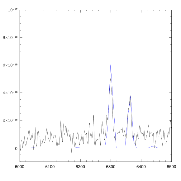
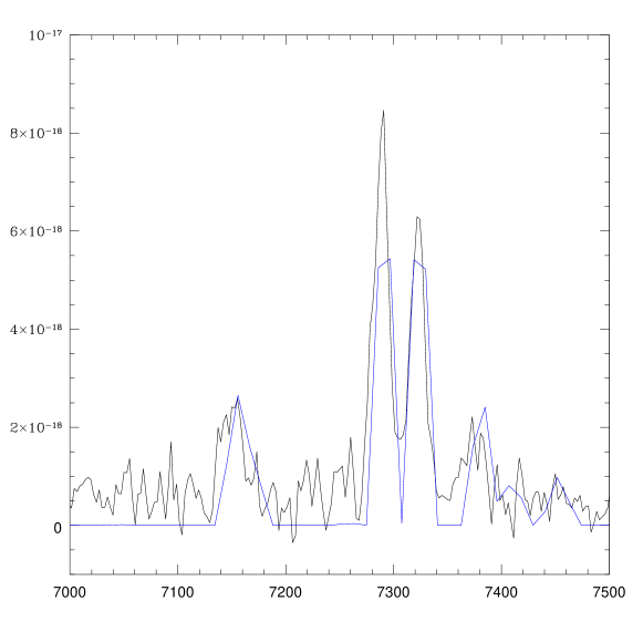
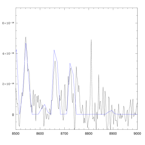
Figure 8: Three snapshots of the modeling (in blue) of the nebular spectrum of SN 2018hwm (in black), fitting the three most important features of the spectrum. From left to right: [O I] doublet, [Ca II] doublet and NIR Ca II triplet. From the model we confirmed the ejected M(⁵⁶Ni) of 0.002 $M_{\odot}$ derived from the hydrodynamical simulation, and estimated the ejected masses of ¹⁶O, ¹²C and ⁴⁰Ca.

In order to establish the properties of the core of the exploding star, we modelled the nebular spectrum with a non-local thermodynamic equilibrium (NLTE) code. The code is based on the assumptions set forth by Axelrod (1980), and it has been described and used in several papers (e.g. Mazzali et al. 2017, 2020). The ejecta are heated and ionised by impact with the products of the radioactive decay chain ⁵⁶Ni-⁵⁶Co-⁵⁶Fe. Cooling occurs mostly via forbidden line emission. If we exclude the H and He envelopes, the heavier elements that are found in the CO core can be modelled independently. Although Fe lines are not visible in the noisy spectrum, we can set the ⁵⁶Ni mass to the value obtained from the light curve, adapt the M(⁵⁶Ni) by verifying that the resulting Fe emission in the region of 4000-5500 Å does not exceed the observed flux, and test the masses of some of the emitting elements. It is immediately clear that all emission lines from heavy elements are very narrow. A typical nebular velocity of 500 kms^-1 appropriately describes their width, so we assume that is the size of the emitting core. The strongest lines we address are [O I] 6300, 6363, [Ca II] 7321, Ca II IR, Mg I] 4571, [C II] 8600.

Three snapshots of the comparison between the model spectrum with the observed one, around the [O I], [Ca II] doublets and NIR Ca II triplet, are shown in Figure 8. By approximating to the blue emission we obtained a M(⁵⁶Ni) of 0.002 $M_{\odot}$. The inferred oxygen and carbon masses are low, M(¹⁶O)$\approx 0.02$ $M_{\odot}$ and M(¹²C)$\approx 0.005M_{\odot}$, respectively. The newly synthesized M(¹⁶O) found for SN 2018hwm is very close to that obtained for SN 2005cs (0.016 $M_{\odot}$, Jerkstrand et al. 2018). This agrees with the findings that MS stars in the 8-12 $M_{\odot}$ range synthesize low amount of oxygen (a few $10^{-2}$ $M_{\odot}$, Nomoto 1984; Woosley & Weaver 1986; Woosley, Langer & Weaver 1995; Chugai & Utrobin 2000).

We require a high ejected calcium mass, $\sim$0.3 $M_{\odot}$, to match the strong observed emission. The Ca lines are not broader than the O line, so it is unlikely that any other region contributes significantly to the emission. In order to achieve the correct ratio of the Ca II lines we need to use a rather strong degree of clumping (filling factor 0.02-0.05), which likely reflects the actual conditions in the young SN remnant. A high M(⁴⁰Ca) is problematic within the ECSN scenario, as theoretical nucleosynthesis calculations predict much lower values ($<$0.01 $M_{\odot}$, Nomoto et al. 2006). As a reference, the 12 $M_{\odot}$ model of Maguire et al. (2012) for SN 2008bk synthesised 2.4E-03 $M_{\odot}$ of calcium. However, a high Ca abundance has been observed in a number of so-called ‘Ca-rich’ transients (e.g. Perets et al., 2010, with M(Ca)=0.135 $M_{\odot}$). Those are more likely to be He-shell detonations on white dwarfs, although Kawabata et al. (2010) suggest two scenarios to explain the Ca-rich Type Ib SN 2005cz: the core-collapse of a low-mass 8-12 $M_{\odot}$ star in a binary system, or an ECSN explosion induced by the merging of a ONeMg and a He white dwarf.

We can conclude that the ejected mass is quite small, and the explosion energy is very low, but it is difficult to distinguish between ECSN and a low-mass Fe-CCSN scenario based solely on the nucleosynthesis. For example, Wanajo et al. (2018) proved that the collapse of a ONeMg core and the least massive Fe-core lead to similar nucleosynthesis. Hence, with the available data, we cannot securely discriminate between EC and Fe-CC scenarios.

The number of LL SNe IIP with extensive coverage both in photometry and spectroscopy allowing detailed modelling is still limited. The number of LL SNe IIP with progenitor information inferred from the direct analysis of pre-explosion HST images is even lower. However, with the available sample, there is a growing evidence that the masses of the progenitors of LL SNe IIP are too low to comfortably match the expectations for a fall-back SN scenario, whereas relatively low-mass RSG leading to an Fe core-collapse or SAGBs producing EC SN explosions are viable alternatives.

Data availability

The data underlying this article are available in the article and in its online supplementary material.

Appendix: Photometry tables

Table A1: Sloan $griz$ AB magnitudes of SN 2018hwm.

Date	MJD	$g$	$r$	$i$	$z$	Instrument
2018/11/01	58423.49	$>$20.9	$>$20.9	-	-	ZTF
2018/11/04	58426.48	18.32 0.05	18.62 0.03	-	-	ZTF
2018/11/07	58429.49	18.38 0.06	18.48 0.05	-	-	ZTF
2018/11/08	58430.41	18.32 0.05	-	-	-	ZTF
2018/11/09	58431.25	18.36 0.01	18.40 0.01	-	-	DECAM
2018/11/10	58432.48	18.60 0.04	18.50 0.04	-	-	ZTF
2018/11/13	58435.52	-	18.53 0.09	-	-	ZTF
2018/11/16	58438.49	18.75 0.05	18.60 0.04	-	-	ZTF
2018/11/17	58439.41	18.74 0.05	18.59 0.03	-	-	ZTF
2018/11/19	58441.44	18.86 0.04	18.65 0.03	-	-	ZTF
2018/11/20	58442.38	-	18.76 0.08	-	-	ZTF
2018/11/25	58447.42	-	18.60 0.08	-	-	ZTF
2018/11/26	58448.43	-	18.65 0.08	-	-	ZTF
2018/12/09	58461.47	19.37 0.15	18.56 0.03	-	-	ZTF
2018/12/13	58465.51	19.35 0.08	18.71 0.04	-	-	ZTF
2018/12/16	58468.46	19.34 0.06	18.58 0.03	-	-	ZTF
2018/12/20	58472.45	19.59 0.14	18.77 0.03	-	-	ZTF
2018/12/28	58480.45	19.45 0.17	18.53 0.12	-	-	ZTF
2018/12/29	58481.43	-	18.48 0.04	-	-	ZTF
2019/01/04	58487.44	19.27 0.10	18.64 0.04	-	-	ZTF
2019/01/07	58490.09	-	18.57 0.11	-	-	ALFOSC
2019/01/12	58495.26	19.44 0.09	-	-	-	ZTF
2019/01/15	58498.00	-	18.44 0.04	-	-	ALFOSC
2019/01/26	58509.26	19.33 0.13	18.64 0.06	-	-	ZTF
2019/02/09	58523.23	19.44 0.12	18.65 0.03	-	-	ZTF
2019/02/12	58526.31	19.34 0.23	18.69 0.06	-	-	ZTF
2019/02/20	58534.28	-	18.57 0.16	-	-	ZTF
2019/02/21	58535.95	-	18.64 0.06	-	-	ALFOSC
2019/02/24	58538.25	19.81 0.24	-	-	-	ZTF
2019/02/26	58540.93	19.65 0.04	18.68 0.02	18.53 0.02	18.52 0.04	IO:O
2019/03/02	58544.88	19.48 0.05	18.70 0.02	18.56 0.03	18.54 0.07	IO:O
2019/03/06	58548.03	-	-	18.70 0.08	18.33 0.11	APOGEE
2019/03/06	58548.84	19.63 0.06	18.71 0.03	18.54 0.03	18.56 0.05	IO:O
2019/03/11	58553.89	19.82 0.06	18.84 0.02	18.65 0.03	18.57 0.04	IO:O
2019/03/13	58555.85	20.30 0.04	18.91 0.03	18.80 0.02	18.62 0.02	IO:O
2019/03/15	58557.02	-	18.90 0.10	-	-	APOGEE
2019/03/16	58558.23	-	18.98 0.11	-	-	ZTF
2019/03/17	58559.03	-	-	19.04 0.16	18.64 0.30	APOGEE
2019/03/19	58561.87	20.16 0.29	19.35 0.18	18.97 0.09	18.79 0.12	IO:O
2019/03/25	58567.17	20.95 0.20	-	-	-	ZTF
2019/04/02	58575.17	20.98 0.23	-	-	-	ZTF
2019/04/07	58580.89	-	-	20.52 0.04	20.33 0.05	ALFOSC
2019/04/13	58586.97	21.37 0.36	20.51 0.06	20.82 0.12	20.69 0.14	IO:O
2019/04/15	58588.89	21.49 0.06	20.72 0.04	20.87 0.04	20.79 0.06	ALFOSC
2019/04/25	58598.17	21.25 0.26	21.12 0.19	-	-	ZTF
2019/04/28	58601.87	22.69 0.15	21.25 0.04	20.75 0.05	20.94 0.07	ALFOSC
2019/05/14	58617.87	-	21.28 0.05	20.94 0.07	-	ALFOSC
2019/10/04	58760.25	-	22.24 0.09	-	-	ALFOSC
2019/11/27	58814.20	-	22.85 0.13	-	-	OSIRIS

Table A2: Johnson $BVRI$ Vega magnitudes of SN 2018hwm.

Date	MJD	$B$	$V$	$R$	$I$	Instrument
2018/11/08	58430.33	-	18.43 0.03	-	-	EFOSC
2019/01/10	58493.23	19.90 0.06	18.70 0.03	-	-	ANDICAM
2019/01/15	58498.24	19.96 0.07	18.72 0.04	-	17.93 0.03	ANDICAM
2019/01/24	58507.19	20.04 0.10	18.83 0.07	-	17.90 0.04	ANDICAM
2019/02/01	58515.19	20.20 0.07	18.76 0.03	-	17.96 0.04	ANDICAM
2019/02/03	58517.27	20.22 0.08	18.79 0.07	18.23 0.06	17.89 0.08	Fairchild
2019/02/08	58522.15	20.17 0.06	18.81 0.05	-	17.92 0.08	ANDICAM
2019/02/16	58530.14	20.26 0.10	19.06 0.16	-	17.92 0.09	ANDICAM
2019/02/22	58536.23	-	19.03 0.06	18.44 0.05	-	Fairchild
2019/02/23	58537.15	-	18.93 0.05	18.38 0.04	18.03 0.03	ANDICAM
2019/02/26	58540.89	20.38 0.08	19.13 0.03	-	-	IO:O
2019/03/02	58544.88	20.39 0.09	19.09 0.04	-	-	IO:O
2019/03/06	58548.12	-	19.05 0.04	18.49 0.04	18.11 0.10	ANDICAM
2019/03/06	58548.85	20.72 0.11	19.53 0.06	-	-	IO:O
2019/03/11	58553.90	20.77 0.13	19.47 0.05	-	-	IO:O
2019/03/15	58557.92	20.96 0.21	19.54 0.09	-	-	IO:O
2019/03/19	58561.87	-	19.72 0.23	-	-	IO:O
2019/03/22	58564.11	-	19.82 0.15	19.19 0.09	18.90 0.15	Fairchild
2019/04/03	58576.06	-	20.60 0.14	20.10 0.10	-	ANDICAM
2019/04/06	58579.07	-	20.65 0.11	20.08 0.14	-	ANDICAM
2019/04/09	58582.05	-	20.70 0.14	20.09 0.13	-	ANDICAM
2019/04/15	58588.88	-	21.40 0.11	20.46 0.05	-	ALFOSC
2019/04/28	58601.86	-	21.37 0.08	-	-	ALFOSC
2019/05/14	58617.87	-	21.36 0.11	-	-	ALFOSC

Table A3: NIR $JHKs$ Vega magnitudes of SN 2018hwm.

Date	MJD	$J$	$H$	$Ks$	Instrument
2019/01/11	58494.21	17.36 0.03	17.08 0.02	17.01 0.05	NOTCAM
2019/01/29	58512.99	17.43 0.02	17.13 0.02	16.91 0.03	NOTCAM
2019/03/04	58546.93	17.80 0.03	17.40 0.03	17.21 0.05	NOTCAM
2019/03/21	58563.97	19.09 0.08	18.39 0.07	-	NOTCAM

References

- Anderson et al. (2014) Anderson J.P., González-Gaitán S. et al., 2014, ApJ, 786, 67
- Arcavi et al. (2012) Arcavi I., Gal-Yam A., Cenko S. B. et al., 2012, ApJ, 756, 30
- Asplund et al. (2009) Asplund M., Grevesse N. et al., 2009, ARA&A, 47, 481
- Axelrod (1980) Axelrod T. S.,1980, PhDT, 1A
- Barbon, Ciatti & Rosino (1979) Barbon R., Ciatti F. & Rosino L., 1979, A&A, 72, 287
- Bellm et al. (2019) Bellm E. C., Kulkarni S. R. et al., 2019, PASP, 131, 8002
- Benetti et al. (2001) Benetti S., Turatto T., Balberg S. et al., 2001, MNRAS, 322, 361
- Bersten et al. (2011) Bersten M. C., Benvenuto O., Hamuy M., 2011, ApJ, 729, 61
- Blagorodnova et al. (2018) Blagorodnova N., Neill J. D. et al., 2018, PASP, 130, 5003
- Blondin & Tonry (2007) Blondin S. & Tonry J. L., 2007, ApJ, 666, 1024
- Burrows et al. (2020) Burrows A., Radice D., Vartanyan D., 2020, MNRAS, 491, 2715
- Cappellaro (2014) Cappellaro E., 2014, SNOoPY: a package for SN photometry, http://sngroup.oapd.inaf.it/snoopy.html
- Cardelli, Clayton & Mathis (1989) Cardelli, J.A.; Clayton, G.C.; Mathis, J.S., 1989, ApJ, 345, 245
- Chugai & Utrobin (2000) Chugai N. N. & Utrobin V. P., 2000, A&A, 354, 557
- Congiu et al. (2018) Congiu E., Berton M., Benetti S. et al., 2018, ATel 12191
- De Vaucouleurs (1991) De Vaucouleurs G., De Vaucouleurs A. et al., 1991, RC3
- Doherty et al. (2017) Doherty C. L., Gil-Pons P. et al., 2017, PASA, 34, 56
- Eldridge, Mattila & Smartt (2007) Eldridge, J. J., Mattila, S., Smartt, S. J., 2007, MNRAS, 376, 52
- Falco et al. (1999) Falco E. E., Kurtz M. J. et al., 1999, PASP, 111, 438
- Faran et al. (2014a) Faran T., Poznanski D. et al. 2014, MNRAS, 442, 844