Sparse Inpainting with Smoothed Particle Hydrodynamics

Abstract

Digital image inpainting refers to techniques used to reconstruct a damaged or incomplete image by exploiting available image information. The main goal of this work is to perform the image inpainting process from a set of sparsely distributed image samples with the Smoothed Particle Hydrodynamics (SPH) technique. As, in its naive formulation, the SPH technique is not even capable of reproducing constant functions, we modify the approach to obtain an approximation which can reproduce constant and linear functions. Furthermore, we examine the use of Voronoi tessellation for defining the necessary parameters in the SPH method as well as selecting optimally located image samples. In addition to this spatial optimization, optimization of data values is also implemented in order to further improve the results. Apart from a traditional Gaussian smoothing kernel, we assess the performance of other kernels on both random and spatially optimized masks. Since the use of isotropic smoothing kernels is not optimal in the presence of objects with a clear preferred orientation in the image, we also examine anisotropic smoothing kernels. Our final algorithm can compete with well-performing sparse inpainting techniques based on homogeneous or anisotropic diffusion processes as well as with exemplar-based approaches.

65D18, 68U10, 76M28, 94A08

1 Introduction

Image inpainting aims at restoring partially damaged image or missing parts of an image in a visually appealing manner [9]. It has a wide number of practical applications such as art restoration [47, 6, 19, 72], object removal [27], medical imaging [83], inpainting of optical flow fields [71], video inpainting [63], inpainting reflectance/height values in LiDAR images [12, 26], image compression [38, 74], and even image denoising [2]. The term “inpainting” itself was introduced for digital images by Bertalmío et al. in [9], but similar concepts were already explored in earlier work under different names such as image restoration, interpolation, disocclusion, or amodal completion [45, 65, 36, 20, 59].

Any inpainting model needs to assume some kind of relation between known and unknown data. As there is a variety of plausible assumptions for such relations, many solutions to an inpainting problem exist.

Based on the underlying assumptions, the inpainting methods from the literature can be grouped into certain main categories [8, 40]. One class is based on variational models and partial differential equations (PDEs) [75], comprising e.g. Euler’s elastica [64, 59, 22, 16, 21], transport-like equations [9, 14], anisotropic diffusion processes [88, 38, 15], harmonic and biharmonic inpainting [23, 38], total variation restoration [23], the Mumford-Shah functional [23, 33], and the Cahn–Hilliard equation [11, 18]. Exemplar-based approaches emerged from texture synthesis and exploit the notion of patch similarity [30, 27, 34, 4]. Other techniques rely on overcomplete dictionaries and the concept of sparsity [32, 58, 31], and more recently also deep learning concepts have been proposed [66, 46, 85]. Each of these strategies has its advantages and disadvantages depending on the type of image it is applied to. For example, exemplar-based techniques perform fairly well on highly textured images, PDE-based methods are more suited for geometrical structures, and deep learning approaches can capture high-level semantics from images. This has led to the development of hybrid approaches which combine the strengths of different methods [10, 80, 5, 70].

A subclass of inpainting problems deals with the recovery of a whole image from a small amount of sparsely distributed data [1, 15, 34, 42]. These kind of problems are encountered particularly in the context of compression [38, 25, 74, 68]. The sparsity of available data makes it feasibly to consider scattered data interpolation, e.g. by radial basis functions [55, 90, 84, 35, 50, 26] or by Shepard interpolation [78, 49, 1, 68] as inpainting technique.

A key observation for applications in compression is that the data can be chosen freely from the image. Thus, a careful selection of the sparse set of pixels to store such that it fits a chosen inpainting method is essential for a good performance [38, 57, 25, 74, 42, 48]. Astonishingly, simple linear methods such as homogeneous diffusion inpainting show remarkable quality if combined with optimally chosen data [7, 38, 43, 25, 69, 13] and can even compete with the widely used JPEG [67] and JPEG2000 [82] standards [56, 44, 69]. Anisotropic diffusion approaches perform even better [38, 74, 42] and can outperform JPEG and JPEG2000 for high compression ratios.

1.1 Goals and Contributions

The goal of our paper is to show that a hitherto hardly explored class of scattered data interpolation methods based on Smoothed Particle Hydrodynamics (SPH) can provide excellent results on sparse inpainting problems, if one improves them with a number of refined concepts.

SPH was originally introduced to solve astrophysical problems [54], but has also been applied to problems that deal with large deformations [17], computational fluid mechanics [61], and soil mechanics [60]. In SPH, the solution to a given problem is represented by a set of particles and functions. Derivatives and integrals are approximated using those particles.

Di Blasi et al. [29] have introduced the SPH method for sparse image interpolation problems, and applications to non-sparse inpainting are studied in [3]. We have not found more work on SPH-based image inpainting. One reason for this lack of popularity might lie in the fact that in the naive formulation, not even constant functions are interpolated correctly [35]. However, in our paper we show that one can come up with highly competitive approaches by integrating more sophisticated concepts. The modifications that we apply are mostly tailored to the particular situation encountered when inpainting is used as a strategy for compression. Compared to other, more classical applications of inpainting, the key difference when using inpainting for compression is that a ground truth image is known, such that the data used for inpainting can be adapted and optimized with regard to this ground truth. Moreover, compression applications are particularly challenging, since they keep only a very sparse subset of the original data.

Our key contributions are the following:

1. To define a measure for the area of influence of a given particle (mask point), we combine a Voronoi tessellation with the Euclidean distance transform.

2. We restore particle consistency.

3. We perform inpainting with a new method that adapts its consistency order to the local approximation error.

4. We use the Voronoi tessellation to propose a novel strategy for spatial data optimization.

5. We optimize not only the data locations, but also their values (tonal optimization).

6. To incorporate anisotropy in the process, we use anisotropic kernels.

7. We assess the performance of different smoothing kernels and compare to some of the best sparse inpainting methods for optimized data.

In the context of image processing and reconstruction, related concepts have been used in combination with kernel regression methods, e.g., by Takeda et al. in [81].

1.2 Paper Structure

This paper is organized as follows: In Section 2, we give a brief summary of the ideas behind Smoothed Particle Hydrodynamics. This includes its origin from an integral approximation, techniques to restore consistency in a discrete setting, and a brief overview on common smoothing kernels used for our experiments. Section 3 explains how SPH can be used for inpainting. Here we introduce Voronoi tessellation to determine parameters of the method. Further, we compare performance of SPH inpainting with diffusion- and exemplar-based methods for examples of sparse inpainting and classical inpainting tasks. For problems in which the ground truth is known, we show how performance can be enhanced by combining results from methods of different consistency order in Section 4. Here, we also explain our data optimization strategies both with respect to data locations (spatial optimization) as well as data values (tonal optimization). We proceed by comparing results from our method to results from other techniques in Section 4.6 and draw conclusions in Section 5.

2 SPH in a Nutshell

2.1 Essential Ideas

We are interested in approximating a function $f$ on the domain $\Omega$ in $\mathbb{R}^{2}$. The point of departure for SPH is the idea to replace the value of $f$ at a point $\bm{q}$ by a weighted average of the function, i.e.

(1) $$f\!\left(\bm{q}\right)\approx\left\langle f\!\left(\bm{q}\right)\right\rangle\coloneqq\int_{\Omega}f\!\left(\bm{p}\right)\,W\!\left(\bm{q}-\bm{p},h\right)\,\mathrm{d}\bm{p}.$$

Equation 1 is also known as the kernel approximation of the function with the smoothing kernel $W(\cdot,h)$ and its smoothing length $h$, which represents the effective width of $W$. The kernel should be a monotonically decreasing positive mollifier, i.e. it should have the following properties:

• compactness: $W(\bm{q}-\bm{p},h)=0$ outside a compact domain $K\subseteq\Omega$,

• unity: $\int_{\Omega}W(\bm{q}-\bm{p},h)\,\mathrm{d}\bm{p}=1$,

• limit behavior: $W(\bm{q}-\bm{p},h)\xrightarrow{h\rightarrow 0}\delta(\bm{q}-\bm{p})$, where $\delta(\bm{q}-\bm{p})$ is Dirac’s delta distribution,

• positivity: $W(\bm{q}-\bm{p},h)>0$ over $K\subseteq\Omega$,

• monotonicity: $W$ is monotonically decreasing function w.r.t. $\left\lVert\bm{q}-\bm{p}\right\rVert$.

Here, $\lVert\cdot\rVert$ denotes the Euclidean distance. Positivity is not strictly necessary, but desired in order for the approximated function values to have physical meaning. Allowing the kernel to take negative values in parts of the domain can lead to unnatural approximated values and corrupt the entire computation [52]. The same holds for monotonicity, which is connected with the usual behavior of physical forces to decrease with increasing distance.

Discretizing the integral of Eq. 1 yields the particle approximation of $f$ given by

(2) $$f\!\left(\bm{q}\right)\approx u\!\left(\bm{q}\right)\coloneqq\sum\limits_{j\in\mathcal{N}(\bm{q})}f\!\left(\bm{p}_{j}\right)\,W\!\left(\bm{q}-\bm{p}_{j},h\right)\,V_{j}.$$

Here, in order to approximate the function value at point $\bm{q}$ we sum over its nearest neighbors $\bm{p}_{j}$, where $\mathcal{N}(\bm{q})$ denotes the index set of the nearest neighbors and we assume that $1\leq j\leq M$ with $M$ the total number of particles under consideration. Each of these particles is related to a specific area of influence (or weight) $V_{j}$ in this quadrature rule. The particle approximation is interpolating at the particles $\bm{p}_{j}$ if the kernel $W$ satisfies

(3) $$W\!\left(\bm{p}_{k}-\bm{p}_{j},h\right)\,V_{j}=\delta_{k,j}\quad\text{for any}\quad j,k=1,\ldots,M$$

with the Kronecker delta $\delta_{k,j}$. This requirement is separate from the desired properties in the continuous setting and, in general, not satisfied by kernels with said properties. Some modifications which achieve interpolation at the particles are discussed in Section 2.2.

In order to determine the nearest neighbors, we use the so-called scatter approach. Here, the neighbors of a point $\bm{q}$, are the particles $\bm{p}_{j}$ that include $\bm{q}$ in the support domain of the kernels centered at these particles $\bm{p}_{j}$, cf. Fig. 1.

Figure 1: Particles $\bm{p}_{1}$, $\bm{p}_{2}$, and $\bm{p}_{3}$ are considered neighbors of point $\bm{q}$, while $\bm{p}_{4}$ is not.

An alternative to the scatter approach is the gather approach [51] in which a disk of a predetermined radius around $\bm{q}$ is considered and neighbors are determined by checking which particles $\bm{p}_{j}$ are located within the disk. The scatter approach is preferable for our purpose as it is less dependent on the particle distribution and allows to consider different smoothing lengths $h_{j}$ for each particle.

2.2 Restoring Consistency

Consistency in SPH is defined in the sense of (local) polynomial reproduction [90]. While the restriction of kernels to positive mollifiers guarantees that linear polynomials are reconstructed in the continuous formulation Eq. 1, this is no longer the case in the discrete formulation Eq. 2; a phenomenon known as particle inconsistency [62]. Thus, Eq. 2 needs to be modified in order to restore consistency in the discrete setting.

For the particle approximation to satisfy zero order consistency, it needs to be able to reproduce constants. This requirement is satisfied by the well known Shepard interpolation formula [78, 24, 90]

(4) $$u\!\left(\bm{q}\right)=\frac{\sum\limits_{j\in\mathcal{N}(\bm{q})}f\!\left(\bm{p}_{j}\right)\,W\!\left(\bm{q}-\bm{p}_{j},h\right)\,V_{j}}{\sum\limits_{j\in\mathcal{N}(\bm{q})}W\!\left(\bm{q}-\bm{p}_{j},h\right)\,V_{j}}.$$

The fact that zero order consistency already requires to modify Eq. 2 shows that, in general, using the particle approximation directly cannot even reproduce constant functions, i.e. Eq. 2 has no consistency.

One way to interpret Shepard interpolation is that the kernel $W$ is replaced by a modified kernel $\widetilde{W}$ such that

(5) $$\widetilde{W}\!\left(\bm{q}-\bm{p}_{j},h\right)=b_{0}\!\left(\bm{q}\right)\,W\!\left(\bm{q}-\bm{p}_{j},h\right),$$

and the original interpolation formula is used with the modified kernel, i.e.,

(6) $$u\!\left(\bm{q}\right)=\sum\limits_{j\in\mathcal{N}(\bm{q})}f\!\left(\bm{p}_{j}\right)\,\widetilde{W}\!\left(\bm{q}-\bm{p}_{j},h\right)\,V_{j}.$$

By comparison with Eq. 4, we see that $b_{0}\!\left(\bm{q}\right)$ is given by

(7) $$b_{0}\!\left(\bm{q}\right)=\frac{1}{\sum\limits_{j\in\mathcal{N}(\bm{q})}W\!\left(\bm{q}-\bm{p}_{j},h\right)\,V_{j}}.$$

Thus, $b_{0}\!\left(\bm{q}\right)$ is a function of $\bm{q}$, but is constant with respect to the particle $\bm{p}_{j}$ for a fixed $\bm{q}$. In other words, zero order consistency can be restored by multiplying the kernel by a constant. This motivates the attempt to restore first order consistency by multiplying the kernel with a function which is linear in the difference $\bm{q}-\bm{p}_{j}$, i.e.

(8) $$\widetilde{W}\!\left(\bm{q}-\bm{p}_{j},h\right)=\left(b_{0}\!\left(\bm{q}\right)+b_{1}\!\left(\bm{q}\right)\left(x_{\bm{q}}-x_{\bm{p}_{j}}\right)+b_{2}\!\left(\bm{q}\right)\left(y_{\bm{q}}-y_{\bm{p}_{j}}\right)\right)\,W\!\left(\bm{q}-\bm{p}_{j},h\right),$$

where $\bm{q}=(x_{\bm{q}},y_{\bm{q}})^{T}$ and $\bm{p}_{j}=(x_{\bm{p}_{j}},y_{\bm{p}_{j}})^{T}$. For a fixed $\bm{q}$, this means that we have to determine three coefficients such that we can reproduce linear polynomials in $\mathbb{R}^{2}$. This yields the system of equations

(9) $$\sum\limits_{j\in\mathcal{N}(\bm{q})}\widetilde{W}\!\left(\bm{q}-\bm{p}_{j},h\right)\,V_{j}= \ 1,$$

(10) $$\sum\limits_{j\in\mathcal{N}(\bm{q})}x_{\bm{p}_{j}}\,\widetilde{W}\!\left(\bm{q}-\bm{p}_{j},h\right)\,V_{j}= \ x_{\bm{q}},$$

(11) $$\sum\limits_{j\in\mathcal{N}(\bm{q})}y_{\bm{p}_{j}}\,\widetilde{W}\!\left(\bm{q}-\bm{p}_{j},h\right)\,V_{j}= \ y_{\bm{q}}.$$

Equation 9 allows to multiply the right-hand sides of Eqs. 10 and 11 by the left-hand side of Eq. 9 without changing the equations, such that this linear system can be recast as

(12) $$\bm{D}\!\left(\bm{q}\right)\,\bm{b}\!\left(\bm{q}\right)=\bm{e}$$

if we define

(13) $$\bm{b}\!\left(\bm{q}\right)=\begin{pmatrix}b_{0}\!\left(\bm{q}\right)\\ b_{1}\!\left(\bm{q}\right)\\ b_{2}\!\left(\bm{q}\right)\end{pmatrix},\qquad\bm{e}=\begin{pmatrix}1\\ 0\\ 0\end{pmatrix},\qquad\bm{v}_{j}\!\left(\bm{q}\right)=\begin{pmatrix}1\\ x_{\bm{p}_{j}}-x_{\bm{q}}\\ y_{\bm{p}_{j}}-y_{\bm{q}}\end{pmatrix}.$$

The matrix $\bm{D}\!\left(\bm{q}\right)$ can be expressed as a sum of matrices of rank $1$ in the form

(14) $$\bm{D}\!\left(\bm{q}\right)=\sum\limits_{j\in\mathcal{N}(\bm{q})}W\!\left(\bm{p}_{j}-\bm{q},h\right)\,V_{j}\,\bm{v}_{j}\!\left(\bm{q}\right)\,\bm{v}_{j}^{T}\!\left(\bm{q}\right).$$

It is positive semidefinite as for any $\bm{z}\in\mathbb{R}^{3}$ holds

(15) $$\bm{z}^{T}\bm{D}\bm{z}=\bm{z}^{T}\left(\sum\limits_{j\in\mathcal{N}(\bm{q})}W\!\left(\bm{p}_{j}-\bm{q},h\right)\,V_{j}\,\bm{v}_{j}\bm{v}_{j}^{T}\right)\bm{z}=\sum\limits_{j\in\mathcal{N}(\bm{q})}W\!\left(\bm{p}_{j}-\bm{q},h\right)\,V_{j}\,\left(\bm{v}_{j}^{T}\,\bm{z}\right)^{2}\geq 0,$$

since the smoothing kernel $W(\cdot)$ is nonnegative and $V_{j}>0$. However, $\bm{D}\!\left(\bm{q}\right)$ is singular unless $\bm{q}$ has at least three nearest neighbors which are not collinear.

In order to achieve an SPH interpolation with first order consistency at a pixel $\bm{q}$, it is necessary to solve the $3\times 3$ linear system Eq. 12. To inpaint a whole image from first order SPH interpolation, Eq. 12 needs to be solved for each unknown pixel. With the solution $\bm{b}\!\left(\bm{q}\right)$ of Eq. 12, a first order consistent SPH approximation can be written as

(16) $$u\!\left(\bm{q}\right)=\sum\limits_{j\in\mathcal{N}(\bm{q})}f\!\left(\bm{p}_{j}\right)\,\widetilde{W}\!\left(\bm{q}-\bm{p}_{j},h\right)\,V_{j}=\sum\limits_{j\in\mathcal{N}(\bm{q})}f\!\left(\bm{p}_{j}\right)\,\bm{v}_{j}^{T}\!\left(\bm{q}\right)\,\bm{b}\!\left(\bm{q}\right)\,W\!\left(\bm{q}-\bm{p}_{j},h\right)\,V_{j}.$$

The particular method used here to restore first order consistency was derived in a longer way in [92], whereas other methods that modify the kernel to restore first order consistency can be found in [53, 51]. The method described here has the advantage that it does not involve derivatives of $f$ to restore first order consistency. For image processing, similar techniques were derived from kernel regression in [81].

The benefit of a higher order consistency does not come without a price. The zero order consistent Shepard interpolation Eq. 4 only modifies the kernel such that it satisfies a discrete partition of unity property. With this modified kernel, Shepard interpolation produces the value of $u$ at $\bm{q}$ as a convex combination of the values of $f$ at the neighboring particles $\bm{p}_{j}$. Thus, it prevents over- and undershoots. If we want the first order consistent method Eq. 16 to prevent over- and undershoots, we have to put a restriction on the positions of particles, since we have to satisfy Eqs. 10 and 11. These equations can be written in a compact way as

(17) $$\bm{q}=\sum\limits_{j\in\mathcal{N}(\bm{q})}\bm{p}_{j}\,\widetilde{W}\!\left(\bm{q}-\bm{p}_{j},h\right)\,V_{j}.$$

In an ideal situation, $u$ at $\bm{q}$ would be a convex combination of the values of $f$ at the neighboring particles $\bm{p}_{j}$ with weights given by $\widetilde{W}\!\left(\bm{q}-\bm{p}_{j},h\right)\,V_{j}$. However, Eq. 17 along with Eq. 9 implies that this can only be the case if the position $\bm{q}$ is also a convex combination of the particle positions $\bm{p}_{j}$ with the same weights. In most cases, this condition on the positions of particles is violated. In order to achieve first order consistency regardless of the spatial distribution of particles, the modified kernel $\widetilde{W}$ violates some of the properties defined in Section 2.1. In particular violation of the positivity requirement results in visible artifacts as can be seen in the bottom left block of images in Fig. 5. This phenomenon is also mentioned as violation of a maximum-minimum principle in the context of inpainting in [41].

2.3 Common Smoothing Kernels

In SPH, most smoothing kernels $W$ incorporate the smoothing length as a scaling parameter, such that they can be expressed in the form

(18) $$W\!\left(\bm{q}-\bm{p},h\right)=W\!\left(\frac{\bm{q}-\bm{p}}{h}\right)=W\!\left(\bm{\eta}\right)\qquad\text{with}\qquad\bm{\eta}\coloneqq\frac{\bm{q}-\bm{p}}{h}.$$

Further, it is common to choose radial kernels such that they can be written in the form

(19) $$W\!\left(\bm{q}-\bm{p},h\right)=W\!\left(\bm{\eta}\right)=\frac{\rho}{h^{2}}\,\Phi\!\left(\left\lVert\bm{\eta}\right\rVert\right).$$

Here, $\rho$ is a normalization factor to satisfy the continuous unity property. Probably the most common kernel is of Gaussian type:

(20) $$\Phi\!\left(\left\lVert\bm{\eta}\right\rVert\right)=\exp\!\left(-\epsilon\,\left\lVert\bm{\eta}\right\rVert^{2}\right).$$

However, as the Gaussian does not have a compact support, it is truncated at $\left\lVert\bm{\eta}\right\rVert=1$. Thus, the parameter $\epsilon$ should be chosen in a way that values of the resulting kernel $W\!\left(\bm{\eta}\right)$ for $\left\lVert\bm{\eta}\right\rVert>1$ can be safely neglected. For the value of the Gaussian at $\left\lVert\bm{\eta}\right\rVert=1$, we obtain

(21) $$W\!\left(\bm{\eta}\right)=\frac{\rho}{h^{2}}\qquad\text{if}\qquad\left\lVert\bm{\eta}\right\rVert=1,$$

which inspires the condition

(22) $$W\!\left(\bm{\eta}\right)\leq\frac{0.01}{h^{2}}\qquad\text{if}\qquad\left\lVert\bm{\eta}\right\rVert=1.$$

Together with the continuous unity property, this allows us to determine both parameters $\rho$ and $\epsilon$, such that we use the Gaussian in the form

(23) $$W\!\left(\bm{\eta}\right)=\frac{\epsilon}{\pi\,h^{2}}\,\exp\!\left(-\epsilon\,\left\lVert\bm{\eta}\right\rVert^{2}\right)$$

with $\epsilon=5.09$. Here, we have expressed $\rho$ as a function of $\epsilon$.

An alternative to the Gaussian are Matérn kernels [35]. Contrary to the Gaussian which is arbitrarily often continuously differentiable, Matérn kernels differ in smoothness. The $C^{0}$-Matérn kernel, which is not differentiable but just continuous at $\bm{\eta}=\bm{0}$, is given by

(24) $$W\!\left(\bm{\eta}\right)=\frac{\epsilon^{2}}{2\pi\,h^{2}}\,\exp\!\left(-\epsilon\left\lVert\bm{\eta}\right\rVert\right),$$

for which we chose $\epsilon=6.52$. A higher regularity at $\bm{\eta}=\bm{0}$ can be achieved with the $C^{2}$-Matérn kernel

(25) $$W\!\left(\bm{\eta}\right)=\frac{\epsilon^{2}}{6\pi\,h^{2}}\,\left(1+\epsilon\left\lVert\bm{\eta}\right\rVert\right)\exp\!\left(-\epsilon\left\lVert\bm{\eta}\right\rVert\right),$$

which we use in our experiments with $\epsilon=8.04$.

Although the truncated Gaussian is a common choice, the original SPH paper [54] already introduced a kernel with a compact support, namely

(26) $$W\!\left(\bm{\eta}\right)=\frac{5}{\pi\,h^{2}}\begin{cases}\left(1+3\left\lVert\bm{\eta}\right\rVert\right)\left(1-\left\lVert\bm{\eta}\right\rVert\right)^{3},&\ \left\lVert\bm{\eta}\right\rVert\leq 1,\\ 0,&\ \left\lVert\bm{\eta}\right\rVert>1,\end{cases}$$

which we will call Lucy kernel. Other commonly used kernels with compact support are the cubic spline [52]

(27) $$W\!\left(\bm{\eta}\right)=\frac{120}{14\pi\,h^{2}}\begin{cases}\frac{2}{3}-4\left\lVert\bm{\eta}\right\rVert^{2}+4\left\lVert\bm{\eta}\right\rVert^{3},&\ \left\lVert\bm{\eta}\right\rVert\leq\frac{1}{2},\\ \frac{1}{6}\left(2-2\left\lVert\bm{\eta}\right\rVert\right)^{3},&\ \frac{1}{2}<\left\lVert\bm{\eta}\right\rVert\leq 1,\\ 0,&\ \left\lVert\bm{\eta}\right\rVert>1,\end{cases}$$

and the Wendland $C^{4}$ kernel [90]

(28) $$W\!\left(\bm{\eta}\right)=\frac{3}{\pi\,h^{2}}\begin{cases}\left(35\left\lVert\bm{\eta}\right\rVert^{2}+18\left\lVert\bm{\eta}\right\rVert+3\right)\left(1-\left\lVert\bm{\eta}\right\rVert\right)^{6},&\ \left\lVert\bm{\eta}\right\rVert\leq 1,\\ 0,&\ \left\lVert\bm{\eta}\right\rVert>1.\end{cases}$$

3 SPH Inpainting

For the majority of inpainting problems discussed in this paper, we consider the reconstruction of an image $f$ from a sparse set of values at scattered pixel locations. These locations, called mask points, take the role of particles $\bm{p}_{j}$ for our SPH-inspired inpainting procedure. The set of all mask points is the inpainting mask $\bm{c}$. Exceptions from this setting are the examples of scratch and text removal in Section 3.3, which we include to investigate how SPH inpainting performs for some classical inpainting problems.

3.1 Choosing Influence Areas and Smoothing Lengths

In order to use Eq. 6 for inpainting, whether with the original particle approximation, Shepard interpolation, or the first order consistent method, we still have to determine an area of influence $V_{j}$ for each given mask point $\bm{p}_{j}$. Further, we want to enhance the adaptivity of the method by allowing for different smoothing lengths $h_{j}$ of the kernels centered at the individual particles. This adaptivity is motivated by the results in [29].

A reasonable idea is to assume that the area of influence of a given mask point $\bm{p}_{j}$ is the set of all points which are closer to $\bm{p}_{j}$ than to any other mask point in $\bm{c}$. This idea leads to a Voronoi tessellation of the domain $\Omega$ with seeds given by the mask points. Voronoi cells have been used before in the context of SPH [39, 79] with promising results.

As we are working in a discrete setting where the smallest unit of area is a pixel, a method which determines approximate Voronoi diagrams based on the squared Euclidean distance transform is our tool of choice for this task. This is a rather natural approach since the Voronoi cell $\Omega_{j}$ associated to the mask point $\bm{p}_{j}$ is defined as

(29) $$\Omega_{j}=\left\{\bm{q}\in\Omega\,|\,\left\lVert\bm{q}-\bm{p}_{j}\right\rVert\leq\left\lVert\bm{q}-\bm{p}_{k}\right\rVert\text{ for all }1\leq k\leq M,\,k\neq j\right\}.$$

Given a binary image $g$ which only takes the values $0$ and $\infty$ throughout a domain $\Omega$, the distance transform assigns to each pixel $\bm{q}$ in $\Omega$ its squared distance to the nearest pixel $\bm{p}$ with $g(\bm{p})=0$. In our case, $g$ takes the value $0$ at the mask points and $\infty$ everywhere else. For practical applications, $\infty$ can be replaced by a sufficiently large number. In a two-dimensional domain, the squared distance transform is given by

(30) $$\begin{split}\mathcal{D}(x,y)=&\ \min_{x^{\prime},y^{\prime}}\left\{(x-x^{\prime})^{2}+(y-y^{\prime})^{2}+g(x^{\prime},y^{\prime})\right\}\\ =&\ \min_{x^{\prime}}\left\{(x-x^{\prime})^{2}+\min_{y^{\prime}}\left\{(y-y^{\prime})^{2}+g(x^{\prime},y^{\prime})\right\}\right\}\end{split}$$

such that it can be computed by two consecutive squared distance transforms in one dimension. We used the algorithm from [86, 37] to compute the distance transform, which is shown to have a complexity of $\mathcal{O}(n_{x}\,n_{y})$, where $n_{x}$ and $n_{y}$ are the number of pixels in the image domain $\Omega$ in $x$- and $y$-direction, respectively. For visualization purposes each and every Voronoi cell is depicted with a different color per Voronoi cell in Fig. 2(c).

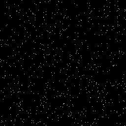
(a) Image with seeds marked in white.

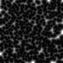
(b) Distance transform.

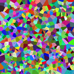
(c) Resulting Voronoi diagram with seeds marked in black.

Figure 2: Voronoi tessellation using distance transform for a given set of mask points $\bm{p}_{j}$ depicted as white seeds in Fig. 2(a). The resulting distance transform is depicted in Fig. 2(b). Corresponding Voronoi cells can be seen in Fig. 2(c), each depicted in a different color with seeds in black now.

After the Voronoi tessellation, each mask point $\bm{p}_{j}$ is assigned as area of influence the area of its corresponding Voronoi cell. In our discrete setting, this area is defined as the sum of pixels that belong to that cell, i.e., pixels are assumed to have area equal to $1$.

It seems natural to determine the smoothing length $h_{j}$ in relation to the volume $V_{j}$, e.g. half the diameter of the Voronoi cell associated to $\bm{p}_{j}$. However, this particular choice is prone to result in pixels for which the requirements of the minimal necessary number of nearest neighbors are not satisfiable. If a pixel does not lie within the support of any kernel, it cannot be inpainted.

A straightforward remedy would be to multiply the diameter of each Voronoi cell with a constant factor chosen such that each pixel has at least the desired minimum number of nearest neighbors. Unfortunately, this would result in oversmoothing and blurring as the resulting kernel supports would be rather large. Instead, we follow the adaptive, iterative approach of [29] for the choice of smoothing lengths, which also enforces that any pixel is inpainted with at least a specified minimum number of neighbors. The scheme starts by assigning each mask point $\bm{p}_{j}$ an initial smoothing length $h_{j,\textrm{init}}$. Using the corresponding kernels, unknown pixels are inpainted, but only if they lie within the support of a least a fixed number of kernels. All pixels which do not satisfy this requirement are not inpainted. Afterwards we check whether there are still pixels with no assigned value left. If so, we increase all smoothing lengths according to a certain rule and try again to inpaint those pixels which are not yet assigned a value. This procedure is repeated iteratively until each pixel is inpainted. As growing strategy for the smoothing lengths, we increase them linearly with the number of iterations.

The original method in [29] assigned initial smoothing lengths which are connected to the choice of $V_{j}$ as made there. However, our experiments showed that it is beneficial if each kernel starts with a minimal smoothing length of $h_{j,\textrm{init}}=1$. Thus, mask points can initially only be recognized as neighbors within a $3\times 3$-patch around them such that the process starts with the smallest sensible isotropic support for each kernel. The smoothing length $h_{j}$ is in each step equal to the number of iterations.

The last parameter that we have to set is the required minimal number of nearest neighbors. For Shepard interpolation, we need at least one neighbor to perform an inpainting, whereas for the method with first order consistency, any pixel must be contained in the support of at least three kernels. For all methods, it is reasonable to choose a slightly larger necessary minimal number of nearest neighbors as this improves results. In particular for the method of first order consistency that reduces the chance to encounter cases in which all mask points closest to an unknown pixel are collinear. For our experiments we require a minimal number of five nearest neighbors.

3.2 Sparse Inpainting on Regular and Random Masks

We follow here a didactic approach and consider the test image “trui” of size $256\times 256$ pixels as an example. Results and comparisons for further images can be found in Section 4.6 and in the supplementary material. All experiments in this paper were performed on an Intel Core i7-9700K CPU @ 3.6GHz.

To get a first impression, we equip the test image with two different types of sparse masks $\bm{c}$. In one case, we choose for $\bm{c}$ a regular mask with a density of $6.25\%$, i.e., pixels on a square grid with a grid width of $4$ pixels are taken as mask points. In the other case, we randomly selected $5\%$ of all image pixels as mask points. Test image “trui” and both masks are shown in Fig. 3.

(a) Original image

(b) 6.25 % regular mask

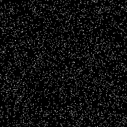
(c) 5 % random mask

Figure 3: The $256\times 256$ test image “trui”, a regular grid of mask points, and a random selection of $5\%$ of image pixels.

In this setting, we perform SPH inpainting with a required minimal number of five neighbors, starting with the kernels given in Section 2.3 and modifying them either according to Shepard interpolation Eq. 4 or the first order consistent method given by Eqs. 12 and 16.

Corresponding results for the case of having a regular mask are depicted in Fig. 4, whereas the results based on the randomly chosen mask points are given in Fig. 5. In order to compare results, all figures give the corresponding mean square errors (MSEs) between the inpainting result and the original image. Further, we have included the runtimes of each set of experiments, averaged across the six different kernels under consideration.

(a) Gaussian $\textrm{MSE}=83.28$ (b) $C^{0}$-Matérn $\textrm{MSE}=83.22$ (c) $C^{2}$-Matérn $\textrm{MSE}=82.03$ (d) Lucy $\textrm{MSE}=81.15$ (e) cubic spline $\textrm{MSE}=78.64$ (f) $C^{4}$-Wendland $\textrm{MSE}=81.94$ (g) Gaussian $\textrm{MSE}=85.01$ (h) $C^{0}$-Matérn $\textrm{MSE}=80.57$ (i) $C^{2}$-Matérn $\textrm{MSE}=80.99$ (j) Lucy $\textrm{MSE}=82.71$ (k) cubic spline $\textrm{MSE}=80.94$ (l) $C^{4}$-Wendland $\textrm{MSE}=79.53$

(m) Harmonic $\textrm{MSE}=121.96$ (n) Biharmonic $\textrm{MSE}=67.95$ (o) EED $\textrm{MSE}=60.68$

Figure 4: Inpainting of “trui” with the 6.25% regular mask from Fig. 3 with a zero order consistency method (top left, (a)-(f)), first order consistency method (bottom left, (g)-(l)), and diffusion-based inpainting (right, (m)-(o)). Inpainting runtime for zero order consistency method was 16.35 s; for first order consistency method 18.26 s (each averaged across all kernels). Parameters for EED are $\lambda=0.2$ and $\sigma=0.8$.

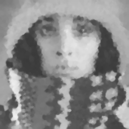
(a) Gaussian $\textrm{MSE}=208.48$ (b) $C^{0}$-Matérn $\textrm{MSE}=206.82$ (c) $C^{2}$-Matérn $\textrm{MSE}=207.85$ (d) Lucy $\textrm{MSE}=219.29$ (e) cubic spline $\textrm{MSE}=223.02$ (f) $C^{4}$-Wendland $\textrm{MSE}=244.35$ (g) Gaussian $\textrm{MSE}=197.58$ (h) $C^{0}$-Matérn $\textrm{MSE}=194.80$ (i) $C^{2}$-Matérn $\textrm{MSE}=195.21$ (j) Lucy $\textrm{MSE}=220.55$ (k) cubic spline $\textrm{MSE}=223.26$ (l) $C^{4}$-Wendland $\textrm{MSE}=287.41$

(m) Harmonic $\textrm{MSE}=226.06$ (n) Biharmonic $\textrm{MSE}=146.46$ (o) EED $\textrm{MSE}=134.92$

Figure 5: Inpainting of “trui” with the 5 % random mask from Fig. 3 with a zero order consistency method (top left, (a)-(f)), first order consistency method (bottom left, (g)-(l)), and diffusion-based inpainting (right, (m)-(o)). Inpainting runtime for zero order consistency method was 3.95 s; for first order consistency method 5.15 s (each averaged across all kernels). Parameters for EED are $\lambda=0.2$ and $\sigma=0.8$.

First of all, comparing the results on the regular mask, we note that the differences are not significant. Further, the higher order of consistency in the bottom left block of images in Fig. 4 is not always beneficial. Indeed, the Gaussian, Lucy kernel, and cubic spline achieve lower MSEs if used in the zero order consistent Shepard interpolation method. Hence, improving consistency in the sense of polynomial reproduction does not automatically yield overall better results. If we only regard the MSE, this stays true for the setting of a random inpainting mask. Here, the performance gains with first order consistency compared to zero order consistency are also not significant whereas for kernels with compact support (Lucy, cubic spline, and $C^{4}$-Wendland) the results are even worse with the first order consistency method.

Comparing the results in Figs. 4 and 5, we observe that further problems arise in the case of a random mask. While for a regular mask, Eq. 17 is satisfied in a way that gives a convex combination on the right-hand side for every unknown pixel $\bm{q}$, this is no longer the case for our random mask. In other words, the modified kernels for a higher order consistency, at pixels whose position cannot be expressed as a convex combination of mask point positions do no longer obey the positivity requirements, resulting in over- and undershoots which can become quite severe. Moreover, the $3\times 3$-system that needs to be solved at each pixel for each modified kernel may become almost singular, leading to further instabilities. For the zero order consistency method, i.e., Shepard interpolation, the $C^{0}$-Matérn kernel yields the best result. This is in line with recent findings by Dell’Accio et al. in [28].

3.3 Classical Inpainting Applications: Scratch and Text Removal

Among the classical applications for inpainting [9] are the removal of scratches or text from an image. Alves Mazzini and Petronetto do Carmo already used SPH inpainting for such tasks in [3]. Thus, we also briefly address such problems here.

As a first example, we consider a damaged version of the image “trui” with scratches, see Fig. 6. To repair those scratches, we consider SPH inpainting of zero and first order consistency for the commonly used Gaussian kernel.

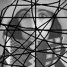
(a) “trui” with scratches

(b) Zero order
$\textrm{MSE}=28.93$

(c) First order
$\textrm{MSE}=23.97$

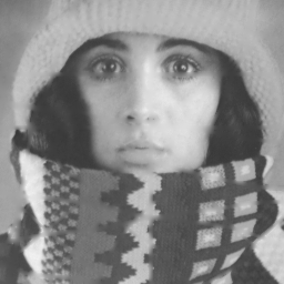
(d) Harmonic
$\textrm{MSE}=23.32$

(e) Biharmonic
$\textrm{MSE}=12.86$

(f) EED
$\textrm{MSE}=12.28$

(g) Exemplar-based
$\textrm{MSE}=49.58$

Figure 6: Image “trui” damaged by scratches (a) and corresponding SPH inpaintings of zero order consistency (b) as well as first order consistency (c) using a Gaussian kernel. Diffusion- and exemplar-based inpainting results are shown in (d-g). Parameters for EED are $\lambda=0.2$ and $\sigma=0.6$.

Regarding MSEs, both methods yield similar results. The differences become clearer when we look at particular areas of the image. For the horizontal scratch below the eyes, we observe visible artifacts in the zero order method while the first order method produces a more pleasing, though not perfect visual impression. On the other hand, for scratches crossing the scarf, the zero order inpainting shows fewer artifacts than the first order inpainting.

As a second example, we consider “trui” overlaid with some text which we attempt to remove in Fig. 7. As before, we use a Gaussian and compare SPH inpainting of zero and first order consistency. For this example, both zero and first order consistency method yield good results, though the first order method is overall slightly better, for example at the boundary between hair and hat on the left-hand side. Overall, both results looks visually pleasant.

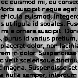
(a) “trui” with text

(b) Zero order
$\textrm{MSE}=18.58$

(c) First order
$\textrm{MSE}=14.27$

(d) Harmonic
$\textrm{MSE}=16.29$

(e) Biharmonic
$\textrm{MSE}=8.72$

(f) EED
$\textrm{MSE}=7.80$

(g) Exemplar-based
$\textrm{MSE}=27.76$

Figure 7: Image “trui” with overlaid text (a) and corresponding SPH inpaintings with zero order consistency (b) as well as first order consistency (c) using a Gaussian kernel. Diffusion- and exemplar-based inpainting results are shown in (d-g). Parameters for EED are $\lambda=0.5$ and $\sigma=0.6$.

3.4 Comparisons with Diffusion-Based and Non-Local Inpainting Methods

To put the results that we have seen so far in perspective, we compare them with the performance of other inpainting methods. As simple representatives of diffusion-based methods, we consider harmonic and biharmonic inpainting [23, 38]. A more sophisticated method is edge-enhancing diffusion (EED). Although introduced as a denoising technique [87], it turned out to be also a powerful inpainting method [38, 69]. For all results shown here and in the supplement, we have used a discretisation of EED which corresponds to the one given in [89] for $\alpha=0$ and $\beta=0$. Contrast parameter $\lambda$ and noise scale $\sigma$ were adapted to the image at hand.

Let us first consider how these methods perform in the case of sparse inpainting masks. The results for the different diffusion based inpainting methods when using the regular inpainting mask from Fig. 3 are included in Fig. 4 on the right. Comparing all results in Fig. 4, we see that, with regard to MSEs, SPH inpainting performs better than harmonic, but worse than biharmonic inpainting. As can be expected, EED shows the best results, both visually and in terms of MSE.

When it comes to inpainting on random masks, the situation is slightly different as Fig. 5 illustrates. Again, the results of the three diffusion-based inpainting methods for the random inpainting mask from Fig. 3 are included on the right. Comparing all results in Fig. 5 shows that the performance of SPH inpainting is similar to harmonic inpainting in terms of MSE, but closer to biharmonic inpainting in terms of visual impression. Again, EED achieves the best MSE and visually smoothest inpainting.

We also compare the results achieved by diffsion-based methods in case of the image damaged by scratches in Fig. 6. Furthermore, we considered the exemplar-based inpainting approach by Criminisi et al. [27] as an example of a non-local inpainting method. For this method, we have considered disc-shaped patches and adapted the patch radius to the image. As is evident from Fig. 6, the first order consistency SPH inpainting can achieve an MSE similar to harmonic inpainting, but shows more artifacts. The exemplar-based method on the other hand is worse with regard to both MSE and creation of artifacts.

Results of the diffusion- and exemplar-based methods in case of the text removal task are included in Fig. 7. The results of SPH inpainting are, once more, similar to the results obtained by harmonic inpainting. The exemplar-based method again produces artifacts, in particular around the eyes.

As a second example, we consider the “parrots” image from the Kodak database, downscaled to size $384\times 256$. As inpainting tasks, we consider the removal of scratches or overlaid texts as well as inpainting based on a sparse regular and a sparse random mask, respectively (see Fig. 8).

(a) Ground truth

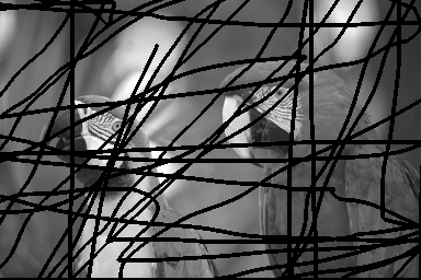
(b) Damaged by scratches

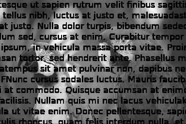
(c) Overlaid with text

(d) 4.16 % regular mask

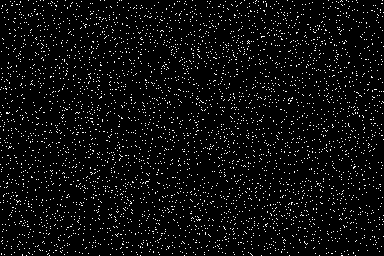
(e) 5 % random mask

Figure 8: Image “parrots” with various inpainting tasks.

Figure 9 shows the results for the inpainting of “parrots” with the regular inpainting masks for SPH inpainting with an isotropic Gaussian and diffusion-based inpainting, whereas results for the random inpainting mask are given in Fig. 10.

(a) Zero order consistency
$\textrm{MSE}=132.79$

(b) First order consistency
$\textrm{MSE}=124.81$

(c) Harmonic
$\textrm{MSE}=139.10$

(d) Biharmonic
$\textrm{MSE}=128.18$

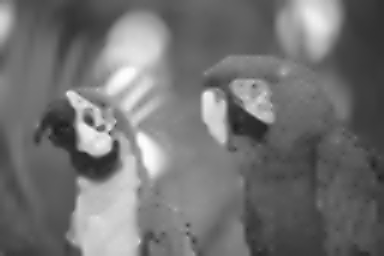
(e) EED
$\textrm{MSE}=118.79$

Figure 9: Inpainting of “parrots” for the regular inpainting mask given in Fig. 8 for various inpainting methods. The SPH inpainting uses a Gaussian kernel. Parameters for EED are $\lambda=1.5$ and $\sigma=2.0$.

(a) Zero order consistency
$\textrm{MSE}=169.62$

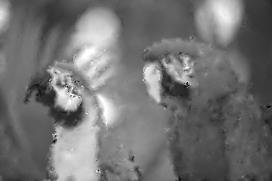
(b) First order consistency
$\textrm{MSE}=173.71$

(c) Harmonic
$\textrm{MSE}=162.53$

(d) Biharmonic
$\textrm{MSE}=147.75$

(e) EED
$\textrm{MSE}=137.04$

Figure 10: Inpainting of “parrots” for the random inpainting mask given in Fig. 8 for various inpainting methods. The SPH inpainting uses a Gaussian kernel. Parameters for EED are $\lambda=1.2$ and $\sigma=2.0$.

For the regular mask, the best MSE is achieved by EED, followed by the first order consistency SPH inpainting. For the random mask, diffusion-based methods show a better performance with EED inpainting taking the lead both with respect to MSE and visual impression. The first order consistency SPH inpainting suffers from the aforementioned artifacts.

Results for the inpainting of image “parrots” damaged by scratches can be found in Fig. 11 whereas Fig. 12 shows the results for text removal.

(a) Zero order consistency
$\textrm{MSE}=37.55$

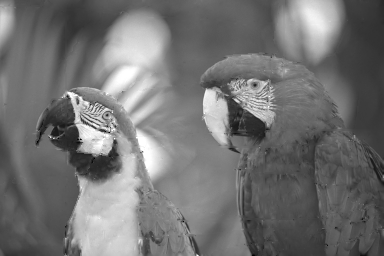
(b) First order consistency
$\textrm{MSE}=44.92$

(c) Exemplar-based
$\textrm{MSE}=76.95$

(d) Harmonic
$\textrm{MSE}=32.94$

(e) Biharmonic
$\textrm{MSE}=28.42$

(f) EED
$\textrm{MSE}=25.70$

Figure 11: Inpainting of “parrots” damaged by scratches (cf. Fig. 8). The SPH inpainting uses a Gaussian kernel. Parameters for EED are $\lambda=0.8$ and $\sigma=1.8$.

(a) Zero order consistency
$\textrm{MSE}=24.00$

(b) First order consistency
$\textrm{MSE}=26.41$

(c) Exemplar-based
$\textrm{MSE}=35.90$

(d) Harmonic
$\textrm{MSE}=21.20$

(e) Biharmonic
$\textrm{MSE}=20.26$

(f) EED
$\textrm{MSE}=17.76$

Figure 12: Inpainting of “parrots” overlaid by text (cf. Fig. 8). The SPH inpainting uses a Gaussian kernel. Parameters for EED are $\lambda=1.2$ and $\sigma=2.0$.

In both tasks, zero order consistency SPH inpainting performs better than the first order consistency method. Both are preferable to the exemplar-based inpainting, but cannot quite achieve the same quality as the diffusion-based approaches. Further results and comparisons are included in the supplementary material.

Overall, we see that SPH inpainting is better suited for inpainting problems with sparse masks, which are closer in nature to the original applications of SPH. Some further remarks on how SPH inpainting may be adapted to non-sparse inpainting tasks, which are out of the scope of this paper, can be found in Section 5. Instead, we focus on how the performance of SPH inpainting can be enhanced in settings which allow data optimization, as they are encountered, e.g., in compression.

4 Optimized Inpainting for Known Ground Truths

4.1 A Mixed Order Consistency Method

The goal of mixed order consistency is to combine zero order and first order consistency to get the best possible result. For this purpose, two inpaintings are done, one with zero order consistency and one with first order consistency. Both results are compared, and the one with the better reconstruction error is kept. The new method is described in Algorithm 1.

Input : Original image $\bm{f}$, mask $\bm{c}$

Output : Reconstruction $\bm{u}$

Initialize : Perform Voronoi tessellation. Assign areas of influence $V_{j}$ to mask points. Assign initial smoothing lengths $h_{j}=h_{j,\textrm{init}}=1$ to mask points. Set $k=1$.

1 while not all pixels $\bm{q}$ have been inpainted do

2       for each pixel $\bm{q}$ do

3             Detect neighboring mask points $\bm{p}_{j}$, $j\in\mathcal{N}(\bm{q})$ of $\bm{q}$.

4             if number of neighbors is larger than or equal to required minimum and neighbors are not collinear then

5                   Inpaint $\bm{q}$ with zero order consistency according to Eqs. 6, 5, and 7.

6                   Inpaint $\bm{q}$ with first order consistency according to Eqs. 8, 12, and 16.

7                   if error of zero order consistency is less than error of first order consistency then

8                         keep inpainting of $\bm{q}$ with zero order consistency,

9                        

10                  else

11                         keep inpainting of $\bm{q}$ with first order consistency.

12                        

13                   end if

14                  

15            else

16                  continue

17             end if

18            

19       end for

20      $k=k+1$

21       $h_{j}=k\cdot h_{j,\textrm{init}}$

22      

23 end while

Algorithm 1 Mixed Consistency Algorithm

Based on the 6.25 % regular mask from Fig. 3, we get the results depicted in Fig. 13, whereas the results for the 5 % random mask are depicted in Fig. 14. For both masks, we have used a minimum of five neighbors. The obtained results are clearly superior to the results achievable with either the zero or first order consistent method, especially for the sparser random mask, showing better MSEs and no visible over- or undershoots.

(a) Gaussian
$\textrm{MSE}=78.37$

(b) $C^{0}$-Matérn
$\textrm{MSE}=67.03$

(c) $C^{2}$-Matérn
$\textrm{MSE}=68.12$

(d) Lucy
$\textrm{MSE}=78.86$

(e) cubic spline
$\textrm{MSE}=72.78$

(f) $C^{4}$-Wendland
$\textrm{MSE}=62.08$

Figure 13: Inpainting of “trui” with the 6.25 % regular mask from Fig. 3 with a mixed order consistency method. Inpainting runtime 19.18 s (averaged across all kernels).

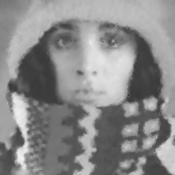
(a) Gaussian
$\textrm{MSE}=128.37$

(b) $C^{0}$-Matérn
$\textrm{MSE}=126.43$

(c) $C^{2}$-Matérn
$\textrm{MSE}=126.36$

(d) Lucy
$\textrm{MSE}=127.07$

(e) cubic spline
$\textrm{MSE}=125.51$

(f) $C^{4}$-Wendland
$\textrm{MSE}=125.02$

Figure 14: Inpainting of “trui” with 5 % random mask from Fig. 3 with a mixed consistency method. Inpainting runtime 5.13 s (averaged across all kernels).

4.2 Spatial Optimization

Our spatial optimization relies on a novel densification strategy. Instead of a probabilistic approach as in [44], we base our method on Voronoi tessellation. The algorithm starts with an empty mask and, as an initial step, inserts the minimum number of neighbors required at random positions. After this step, an initial inpainting takes place and a Voronoi tessellation is performed with the initial mask points as “seeds”. Once this is done, we detect the Voronoi cell with the highest error and insert a new mask point at the pixel with the highest error within the cell. The error of the reconstruction at a pixel $\bm{q}_{j,k}$ in the Voronoi cell $\Omega_{j}$ is defined as

(31) $$E_{\bm{q}_{j,k}}=\left\lvert f\!\left(\bm{q}_{j,k}\right)-u\!\left(\bm{q}_{j,k}\right)\right\rvert^{2},$$

with $f$ being the original image and $u$ the reconstruction, whereas the error for the Voronoi cell $\Omega_{j}$ is given by the sum of the reconstruction errors at all pixels in the cell, i.e.,

(32) $$E_{\Omega_{j}}=\sum\limits_{\bm{q}_{j,k}\in\Omega_{j}}E_{\bm{q}_{j,k}}=\sum\limits_{\bm{q}_{j,k}\in\Omega_{j}}\left\lvert f\!\left(\bm{q}_{j,k}\right)-u\!\left(\bm{q}_{j,k}\right)\right\rvert^{2}.$$

A new inpainting as well as a new Voronoi tessellation are then computed with the new mask and the process continues in the same manner until the required mask density is achieved. The densification algorithm is described in Algorithm 2. We remark that it is possible to insert more than one new mask point in each step to speed up the procedure. However, inserting too many mask points at once deteriorates the quality of the final mask. For the sake of completeness, we also mention that a densification approach using the $\mathrm{L}^{1}$-error within Voronoi cells has been used in [76] for nearest-neighbor and piecewise constant interpolation. In our experiments, using the $\mathrm{L}^{1}$-error always yielded inferior results.

Input : Original image $\bm{f}$, minimum number of neighbors, number of mask points to add per iteration, required density

Output : Mask $\bm{c}$, reconstruction $\bm{u}$

Initialize : Insert minimum number of neighbors at random positions. Perform Voronoi tessellation and initial inpainting.

1 while mask density $<$ required mask density do

2       Find Voronoi cell(s) $\Omega_{j}$ with highest error $E_{\Omega_{j}}$.

3       Find pixel(s) $\bm{q}_{j,k}$ in cell(s) $\Omega_{j}$ with highest error(s) $E_{\bm{q}_{j,k}}$.

4       Add mask point(s) at position(s) $\bm{q}_{j,k}$.

5       Perform Voronoi tessellation.

6       Perform inpainting.

7      

8 end while

Algorithm 2 Densification Algorithm

4.3 Tonal Optimization

Apart from spatial optimization, we also incorporate a gray value optimization of the mask points for a fixed mask $\bm{c}$. The goal of this process is to find the optimal gray values $\bm{g}$ such that the mean square error of the reconstructed image is minimal. Indeed, for a fixed mask $\bm{c}$, the inpainting is given by Eq. 6. However, due to the adaptive nature of the smoothing length $h_{j}$ which is not only determined in dependence of the mask point $\bm{p}_{j}$, but also in dependence of the pixel $\bm{q}$ currently under consideration for inpainting, we have to perform one inpainting for our final mask first to determine all necessary smoothing lengths. Once this is done, Eq. 6 can be written as a matrix vector multiplication of the form $\bm{u}=\bm{A}\widetilde{\bm{f}}$ where $\bm{u}$ is a vector containing the values of the reconstruction at every pixel, $\bm{A}$ is a matrix containing the values of all modified kernels at all pixels multiplied with their area of influence $V_{j}$, and $\widetilde{\bm{f}}$ is a vector containing the values of the original image at all mask points $\bm{p}_{j}$. Thus, as $\bm{A}$ is fixed now, $\bm{u}$ can be interpreted as the solution to an interpolation problem at the mask points. With this interpretation, it is straightforward to consider the corresponding least-squares problem. With the above form for $\bm{u}$, it can be written as

(33) $$\min\limits_{\bm{g}}\left\lVert\bm{A}\bm{g}-\bm{f}\right\rVert^{2},$$

where $\bm{f}$ denotes the vector with the original image values at all pixels and $\bm{g}$ is a vector with gray values at the mask points, which can be determined by solving the normal equations

(34) $$\bm{A}^{T}\bm{A}\bm{g}=\bm{A}^{T}\bm{f}.$$

Although the least squares problem can be solved directly, we prefer an iterative solver instead, specifically the conjugate gradient on the normal residual (CGNR) method [73]. This variant of conjugate gradients avoids the explicit computation of $\bm{A}^{T}\bm{A}$ to reduce runtime and circumvent the larger condition number of $\bm{A}^{T}\bm{A}$ compared to $\bm{A}$. We always initialize by choosing for $\bm{g}_{0}$ the zero vector. As stopping criterion we use a threshold on the relative residual defined such that

(35) $$\frac{\left\lVert\bm{A}^{T}\bm{f}-\bm{A}^{T}\bm{A}\bm{g}_{k}\right\rVert}{\left\lVert\bm{A}^{T}\bm{f}\right\rVert}\leq 10^{-8}.$$

The above procedure is clear for the zero and first order consistency method as they use the same kind of modified kernel in every pixel. It stays valid for the mixed order consistency method as in this approach, the kernel that is used at each pixel $\bm{q}$ is of the same type for all mask points $\bm{p}_{j}$ contributing to the inpainting at $\bm{q}$. Thus, for the mixed consistency method, the type of the modified kernel changes with the rows in $\bm{A}$, but stays the same within each row over all columns. We can still write the whole inpainting process as a matrix-vector-multiplication and solve the associated least-square problem to perform tonal optimization.

4.4 Inpainting on Spatially and Tonally Optimized Data with Isotropic Kernels

As an example for inpainting on an optimized mask with zero order consistency, we present the results produced with a Gaussian kernel in Fig. 15. Even without tonal optimization, the MSE improves by roughly a factor $6.5$. With tonal optimization, the MSE improves by a factor $10$ with respect to the random mask and by almost $35\%$ with respect to the result on the spatially optimized mask without tonal optimization. As far as spatial optimization is concerned, the densification process prefers to capture the geometry of the image, by adding more mask points near edges compared to rather homogeneous regions of the image.

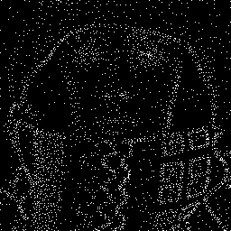
(a) Optimized 5 % mask

(b) $\textrm{MSE}=30.65$

(c) $\textrm{MSE}=19.62$

Figure 15: Inpainting of “trui” with spatially and tonally optimized mask with a zero order consistency method with an isotropic Gaussian kernel. We show the 5 % optimized zero order consistency mask (a), zero order consistency inpainting result with this mask without tonal optimization (b), and zero order consistency inpainting result on this mask with tonal optimization (c). Runtimes were 89.09 min for densification and 2.59 min for tonal optimization.

Changing the SPH inpainting method from zero order consistency to the mixed order consistency method improves the result even further as can be seen in Fig. 16. Using the same isotropic Gaussian kernel as before, spatial optimization improves the MSE by almost a factor $8$ compared to the the random mask result in Fig. 14(a). A comparison with respect to the inpainting method instead of with respect to the mask shows improvement of almost a factor $2$ with respect to the MSE compared to the results in Fig. 15. Unfortunately, there seems to be no structure in the distribution of pixels for which a first order consistency and for which a zero order consistency method performs better, respectively, as can be seen in Fig. 16(b).

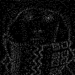
(a) Optimized 5 % mask

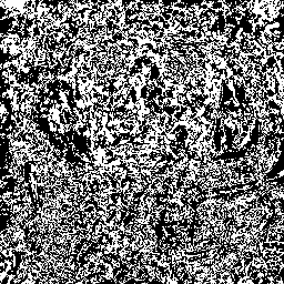
(b) Mixed order consistency map

(c) $\textrm{MSE}=16.30$

(d) $\textrm{MSE}=11.68$

Figure 16: Inpainting of “trui” with spatially and tonally optimized mask with a mixed order consistency method with an isotropic Gaussian kernel. (a) shows an optimized 5 % mask for mixed order consistency SPH inpainting. (b) shows a mixed order consistency map with white areas denoting first order consistency reconstruction and black areas denoting zero order consistency reconstruction. (c) shows a mixed order consistency inpainting result on the mask from (a) without tonal optimization. (d) shows a mixed order consistency inpainting on the same mask with tonal optimization. Runtimes were 111.28 min for densification and 2.66 min for tonal optimization.

Table 1 summarizes MSEs of inpainting results for “trui” with the other isotropic kernels used in Fig. 5 if these kernels are equipped with optimized masks containing $5\%$ of all pixels and tonal optimization is performed.

Kernel	Zero order consistency	mixed order consistency
Gaussian	19.62	11.68
$C^{0}$-Matérn	18.57	9.95
$C^{2}$-Matérn	17.93	9.99
Lucy	21.83	12.15
cubic spline	21.19	11.71
$C^{4}$- Wendland	23.33	11.83

Table 1: MSE comparison between zero and mixed order consistency optimized inpainting with isotropic kernels on “trui” for 5 % masks.

Once again, the benefits of mixed order consistency are quite substantial since a significant decrease of the MSE has been achieved in all cases compared to zero order consistency. Even the best performing kernel for the zero order consistency method, the $C^{2}$-Matérn kernel, has an MSE which is approximately 50 % larger than the MSE of the worst performing kernel in the mixed consistency setting and almost double of the MSE of the best performing kernel in the mixed consistency setting which is the $C^{0}$-Matérn kernel. Further, it appears that compactly supported kernels perform worse in this setting for the zero order consistency SPH inpainting than truncated kernels, but are competitive in the mixed order consistency method.

4.5 Optimized Inpainting with Anisotropic Kernels

The observation that optimized mask points tend to cluster around edges and the fact that edges are clearly oriented structures suggest to adapt the support of kernels to account for this by incorporating anisotropy. This is further supported by results which show that incorporating anisotropy in other inpainting strategies can improve reconstruction quality compared to the related isotropic method [74].

For SPH, anisotropic kernels have been used in the so-called Adaptive Smoothed Particle Hydrodynamics (ASPH) formulation [77] to better account for the actual distribution of particles. Here, we replace the smoothing length $h$ by a symmetric positive definite tensor $\bm{G}\in\mathbb{R}^{2\times 2}$ for a two-dimensional problem and redefine $\bm{\eta}$ as

(36) $$\bm{\eta}=\bm{G}\left(\bm{q}-\bm{p}\right).$$

$\bm{G}$ has units of inverse length and in the isotropic case it is given by a diagonal matrix with each diagonal element equal to $\frac{1}{h}$. This observation makes it clear that we also have to adapt the normalization of our kernels from a factor $\frac{\rho}{h^{2}}$ in Eq. 19 to a factor $\rho\,\det(\bm{G})$.

For SPH inpainting, we determine the anisotropy from the distribution of mask points. For this purpose, we follow the approach of [91] by constructing a weighted local covariance matrix $\bm{C}$ within a fixed predetermined window around each mask point. For a known mask point $\bm{p}_{j}$, the covariance matrix is given by

(37) $$\bm{C}_{j}=\frac{\sum\limits_{\ell}w_{j,\ell}\left(\bm{p}_{\ell}-\widetilde{\bm{p}}_{j}\right)\left(\bm{p}_{\ell}-\widetilde{\bm{p}}_{j}\right)^{T}}{\sum\limits_{\ell}w_{j,\ell}},\qquad\text{ with }\qquad\widetilde{\bm{p}}_{j}=\frac{\sum\limits_{\ell}w_{j,\ell}\,\bm{p}_{\ell}}{\sum\limits_{\ell}w_{j,\ell}}.$$

Here, $\ell$ numbers the mask points within a neighborhood of $\bm{p}_{j}$. It is necessary to restrict the set of mask points under consideration to such a neighborhood to catch the locally prevalent direction of structures in the image. Next, we perform a singular value decomposition (SVD). As $\bm{C}_{j}$ is symmetric and positive semidefinite by construction, this is the same as the eigenvalue decomposition

(38) $$\bm{C}_{j}=\bm{Q}\bm{D}\bm{Q}^{T},$$

with a rotation matrix $\bm{Q}$ and a matrix $\bm{D}$ with nonnegative eigenvalues along the diagonal in decreasing order. As $\bm{C}_{j}$ is constructed from the positions of mask points, its eigenvalues can be assigned a unit of length. The eigenvectors in $\bm{Q}$ correspond to the directions of major and minor axis of an ellipse whose orientation is in line with the locally prevalent orientation in the distribution of mask points. Hence, the tensor $\bm{G}$ is given by

(39) $$\bm{G}=\bm{Q}\bm{D}^{-1}\bm{Q}^{T},$$

such that it has units of inverse length as desired.

In the context of kernel regression, the matrix $\bm{C}$ that we have introduced above is related to the so-called “steering matrix” of an anisotropic regression kernel [81].

In our experiments, we incorporate anisotropy after spatially optimizing mask points for isotropic kernels. We fix the window size for construction of covariance matrices to $25\times 25$ pixels and demand a minimum number of 15 mask points within that window. If this minimum number of mask points is not satisfied, the corresponding kernel stays isotropic. This behavior is desirable since the densification process results in masks where the majority of mask points are placed near discontinuities rather than in homogeneous areas of the image. Thus, a low local density of mask points implies homogeneous areas of the image. The results achieved with mixed order consistency and an anisotropic Gaussian kernel are depicted in Fig. 17.

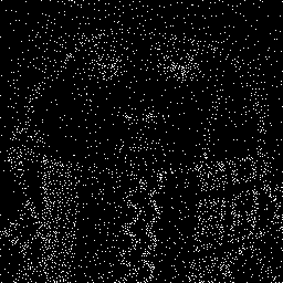
(a) Optimized 5 % mask

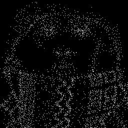
(b) Anisotropic mask points of the 5 % mask

(c) $\textrm{MSE}=10.49$

Figure 17: Inpainting of “trui” with spatially and tonally optimized mask with a mixed order consistency method with an anisotropic Gaussian kernel. From left to right: Optimized 5 % mask for mixed order consistency method (a), mask points which incorporate anisotropic kernels in white (b), and mixed order consistency inpainting result with given mask with tonal optimization (c). Runtimes were 129.44 min for densification and 2.51 min for tonal optimization.

Compared to the result in Fig. 16, we observe an improvement in MSE of only 1.19, which is roughly 11 %, whereas a large amount of mask points is now equipped with anisotropic kernels. This relatively moderate improvement may be explained by the fact that our method of determining anisotropy relies on the local spatial distribution of mask points whereas many important structures in the given image live on a mesoscale. This behavior cannot be captured by increasing the size of the search window as the covariance matrix becomes prone to incorporating the orientations of neighboring structures, resulting in a more isotropic behavior instead of a better orientation along the mesoscale structures. Table 2 summarizes MSEs of inpainting results for “trui” with the other anisotropic kernels used if these kernels are equipped with optimized masks containing $5\%$ of all pixels and tonal optimization is performed.

Kernel	MSE
Gaussian	10.49
$C^{0}$-Matérn	9.51
$C^{2}$-Matérn	9.81
Lucy	11.57
cubic spline	11.26
$C^{4}$- Wendland	11.95

Table 2: MSE with mixed order consistency optimized inpainting with anisotropic kernels on “trui” for 5 % masks.

4.6 Performance Compared to Diffusion-based and Exemplar-based Inpainting Methods

To assess the performance of SPH inpainting, we combine our implementations of harmonic and biharmonic inpainting with our Voronoi-based densification strategy and a tonal optimization approach similar in spirit to Section 4.3. The results achieved by these two inpainting methods are depicted in Fig. 18 together with the corresponding MSEs.

(a) Harmonic
$\textrm{MSE}=20.18$

(b) Biharmonic
$\textrm{MSE}=15.00$

Figure 18: Inpainting of “trui” with spatially and tonally optimized 5 % mask for harmonic and biharmonic inpainting.

As we can see from Table 1, SPH inpainting with mixed order consistency performs better than these two diffusion-based methods even if we consider only isotropic kernels. Table 5 shows that we can obtain an MSE which is less than half that of harmonic inpainting if we incorporate anisotropy.

As another example, consider the “parrots” image from Fig. 8. Figure 19 shows the results obtained by Voronoi densification for a 5 % mask for mixed order consistency SPH inpainting with isotropic and anisotropic Gaussian kernels, including tonal optimization.

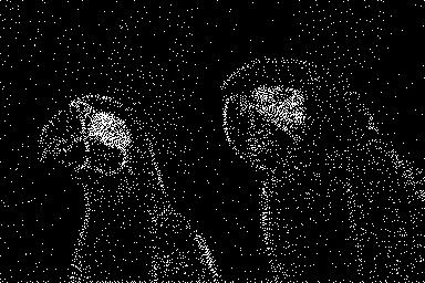
(a) Isotropic mask

(b) Isotropic, mixed order
$\textrm{MSE}=10.07$

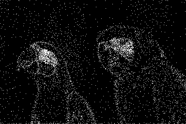
(c) Anisotropic mask

(d) Anisotropic, mixed order
$\textrm{MSE}=8.51$

Figure 19: Inpainting of “parrots” with a 5 % spatially and tonally optimized mask with a mixed order consistency method and Gaussian kernels. Left column shows the masks. Right column shows the inpaintings. Top row is the isotropic case. Bottom row is the anisotropic case.

The corresponding results achieved by harmonic and biharmonic inpainting are shown in Fig. 20.

(a) Harmonic
$\textrm{MSE}=16.44$

(b) Biharmonic
$\textrm{MSE}=15.32$

Figure 20: Inpainting of “parrots” with a 5 % spatially and tonally optimized mask with harmonic (a) and biharmonic (b) inpainting.

Already the isotropic variant of SPH inpainting reduces the MSE of the diffusion-based methods by at least 34 %, whereas the anisotropic version achieves a reduction by 44 %. Further comparisons between SPH inpainting and diffusion-based strategies when equipped with Voronoi-based densification are included in the supplement.

In order to assess the performance of our inpainting method further, we compare it with other existing methods in the literature. As a first example, we consider results for harmonic inpainting on “trui” for an optimized 5 % mask from [57]. There, spatial optimization was done with a probabilistic sparsification and further improved with a Nonlocal Pixel Exchange (NLPE). With optimally chosen mask points and gray values, harmonic inpainting shows an impressive quality in reconstructing the original image. We compare these results with the ones we got for a mixed order consistency SPH inpainting with $C^{0}$-Matérn kernels. To be fair, we only consider isotropic kernels since harmonic inpainting has no way to incorporate anisotropy. The results are summarized in Table 3.

Method	Spatially Optimized	Spatially & Tonally Optimized
Harmonic Inpainting	23.21 (with NLPE)	17.17 (with NLPE)
Mixed SPH (Isotropic)	13.88	9.95

Table 3: MSE for inpaintings of “trui” on optimized 5 % masks. Compared are results achieved with harmonic inpainting in [57] and results from our method with an isotropic $C^{0}$-Matérn kernel with mixed order consistency.

Evidently, we can outperform harmonic inpainting, both without and with tonal optimization. Further results in [57] report MSEs for spatially and tonally optimized harmonic inpainting on the images “peppers” and “walter”. We include these images together with results obtained with mixed order consistency SPH inpainting with isotropic Gaussians in Fig. 21. The MSEs are reported together with those from [57] in Table 4. Again, the results obtained with our method are 16 % and 37 % better, respectively.

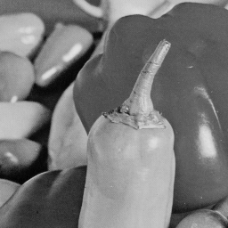
(a) Original image “peppers”

(b) Inpainted “peppers”

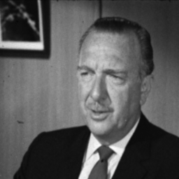
(c) Original image “walter”

(d) Inpainted “walter”

Figure 21: Images “peppers” and “walter” (left column) and mixed order consistency SPH inpaintings with isotropic Gaussian kernels on spatially and tonally optimized 5 % masks (right column).

Image	Harmonic Inpainting	Mixed SPH (Isotropic)
“peppers”	19.38	16.29
“walter”	8.14	5.15

Table 4: MSE for inpaintings on optimized 5 % masks including tonal optimization for images “peppers” and “walter”. Compared are results achieved with harmonic inpainting including NLPE from [57] and results from our method with an isotropic Gaussian kernel with mixed order consistency.

To evaluate SPH inpainting with anisotropic kernels, we consider the results from [42] achieved with edge-enhancing diffusion (EED) inpainting for “trui” with a mask of density 4 % that is constructed by probabilistic sparsification. The authors report the MSE of inpainting on this mask without tonal optimization and improve the location of mask points further with NLPE before considering tonal optimization. As competitor, we used a mixed order consistency SPH inpainting with anisotropic $C^{0}$-Matérn kernels on an optimized 4 % mask. We also tried to improve our inpaintings with NLPE. However, the reduction on MSE was negligible. Results for both inpainting methods are summarized in Table 5.

Method	Spatially Optimized	Spatially + Tonally Optimized
Edge-Enhancing Diffusion (EED)	24.20	10.79 (with NLPE)
Mixed SPH (Anisotropic)	17.10	12.28

Table 5: MSE for inpaintings of “trui” on optimized 4 % masks. Compared are results from EED inpainting [42] and our method with an anisotropic $C^{0}$-Matérn kernel with mixed order consistency.

As can be seen, we outperform EED if we only incorporate spatial optimization, but no tonal optimization. By construction, EED should perform better in preserving edges [87]. Thus, we conjecture that probabilistic sparsification, which only relies on pointwise errors, is inferior to our Voronoi-based densification method as long as the former is not improved by a consecutive NLPE.

To evaluate the performance of our method for images rich in texture, we consider the exemplar-based inpainting technique from [48] and the results given there for an inpainting of a gray value version of the “baboon” image. In this setting, the authors report an MSE of 518.52 on a mask constructed with “densification by dithering” and a consecutive NLPE. As tonal optimization is not considered in [48], we compare to the result our method could achieve for mixed order consistency inpainting with isotropic Gaussians on an optimized 10 % mask in Fig. 22. Already without tonal optimization, the MSE is 290.64, which means we outperform the exemplar-based inpainting method by almost 44 %. Including tonal optimization improves the result further to an MSE of 223.37, less than half of the MSE the exemplar-based method could achieve.

(a) Image “baboon”

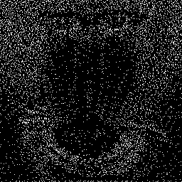
(b) Optimized 10 % mask

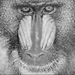
(c) $\textrm{MSE}=290.64$

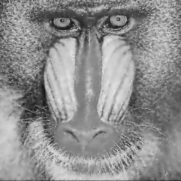
(d) $\textrm{MSE}=223.37$

Figure 22: Inpainting of “baboon” (rescaled to $256\times 256$ pixels as in [48]) with a spatially optimized mask for a mixed order consistency method with an isotropic Gaussian kernel. We show the original image (a), an optimized 10 % mask for mixed order consistency method (b), a mixed order consistency inpainting result with given mask without tonal optimization (c), and a mixed order consistency inpainting result with given mask with tonal optimization. Runtimes were 244.18 min for densification and 5.40 min for tonal optimization.

For the sake of completeness, we also consider the results on “trui” reported for a 10 % masked in [48]. Here, the exemplar-based approach could achieve an MSE of 12.99 with spatial optimization including NLPE. Our mixed consistency SPH inpainting equipped with isotropic Gaussian kernels and a spatially optimized 10 % mask can inpaint “trui” with an MSE of 6.65 which translates to an improvement of 49 %. Tonal optimization decreases the MSE further to 4.68 or an improvement of 64 % compared to the exemplar-based method.

5 Conclusions and Outlook

We have shown that smoothed particle hydrodynamics is a highly competitive method for the challenging problem of sparse data inpainting. It can produce results on par or even better than other, better explored PDE- or exemplar-based inpainting strategies.

The success of SPH for sparse inpainting relies on several novel modifications. With regard to the interpolation procedure, we presented a way to combine the strength of first and zero order methods into a mixed order method. Moreover, we presented a better approach to choose method parameters based on Voronoi tesselations.

The main ingredient to reveal the potential of SPH is the use of optimally chosen data. We proposed a new densification process based on Voronoi tesselations, which lead naturally to a strategy based on a regional error instead of a completely local pointwise error. Thus, a larger amount of data is considered in the optimization procedure, yielding better suitable inpainting masks. Furthermore, we introduced a so far unexplored formulation that allows to use SPH for least-square approximation, i.e., the optimization of data not only in the spatial, but also in the tonal domain. What remains an ongoing topic of research is the question how to choose anisotropies. Taking into account the superior performance of EED, it seems natural to determine anisotropies based on gradient data or the structure tensor. While this is straightforward for regular masks, it becomes more of a challenge for randomly distributed or optimized mask points. In the context of data optimization, one could think about computing anisotropies from the original image. However, for compression purposes, storing this additional data would reduce the rate of compression or necessitate to consider sparser mask, such that there is overall less data to store. On the other hand, when it comes to non-sparse inpainting tasks as briefly touched on in Section 3.3, anisotropies could be determined from the known parts of the image, e.g. by considering gradients similar to [81]. An alternative used for object removal in [41] is to detect edges and their orientation to determine anisotropies from these structures. Both strategies look promising to us when it comes to improving the performance of SPH regarding classical inpainting problems in future research.

We hope that our work will help to give SPH-based inpainting the attention that it deserves. Moreover, we believe that some of our novel concepts, e.g. the Voronoi-based densification for data optimization, will also be useful in applications beyond SPH-based inpainting.

References

- [1] R. Achanta, N. Arvanitopoulos, and S. Süsstrunk, Extreme image completion, in Proc. 42nd IEEE International Conference on Acoustics, Speech and Signal Processing, New Orleans, LA, Mar. 2017, IEEE, pp. 1333–1337.
- [2] R. D. Adam, P. Peter, and J. Weickert, Denoising by inpainting, in Scale Space and Variational Methods in Computer Vision, F. Lauze, Y. Dong, and A. B. Dahl, eds., vol. 10302 of Lecture Notes in Computer Science, Springer, Cham, Switzerland, 2017, pp. 121–132.
- [3] F. Alves Mazzini and F. Petronetto do Carmo, Digital inpainting with SPH method, in Workshop Works in Progress in SIBGRAPI 2016 – Conference on Graphics, Patterns and Images, J. P. Gois and F. Ricardo, eds., São José, Brazil, Oct. 2016.
- [4] P. Arias, G. Facciolo, V. Caselles, and G. Sapiro, A variational framework for exemplar-based image inpainting, International Journal of Computer Vision, 93 (2011), pp. 319–347.
- [5] J.-F. Aujol, S. Ladjal, and S. Masnou, Exemplar-based inpainting from a variational point of view, SIAM Journal on Mathematical Analysis, 42 (2010), pp. 1246–1285.
- [6] W. Baatz, M. Fornasier, P. A. Markowich, and C.-B. Schönlieb, Inpainting of ancient austrian frescoes, in Bridges Leeuwarden: Mathematical Connections in Art, Music, and Science, R. Sarhangi and C. H. Sequin, eds., Tarquin Publications, London, July 2008, pp. 163–170.
- [7] Z. Belhachmi, D. Bucur, B. Burgeth, and J. Weickert, How to choose interpolation data in images, SIAM Journal on Applied Mathematics, 70 (2009), pp. 333–352.
- [8] M. Bertalmío, V. Caselles, S. Masnou, and G. Sapiro, Inpainting, in Computer Vision: A Reference Guide, K. Ikeuchi, ed., Springer, Boston, MA, 2014, pp. 401–416.
- [9] M. Bertalmío, G. Sapiro, V. Caselles, and C. Ballester, Image inpainting, in Proc. 27th Annual Conference on Computer Graphics and Interactive Techniques (SIGGRAPH), New Orleans, LA, July 2000, ACM Press/Addison-Wesley, pp. 417–424.
- [10] M. Bertalmío, L. Vese, G. Sapiro, and S. Osher, Simultaneous structure and texture image inpainting, IEEE Transactions on Image Processing, 12 (2003), pp. 882–889.
- [11] A. L. Bertozzi, S. Esedoglu, and A. Gillette, Inpainting of binary images using the Cahn–-Hilliard equation, IEEE Transactions on Image Processing, 16 (2007), pp. 285–291.
- [12] P. Biasutti, J.-F. Aujol, M. Brédif, and A. Bugeau, Diffusion and inpainting of reflectance and height LiDAR orthoimages, Computer Vision and Image Understanding, 179 (2019), pp. 31–40.
- [13] S. Bonettini, I. Loris, F. Porta, M. Prato, and S. Rebegoldi, On the convergence of a linesearch based proximal-gradient method for nonconvex optimization, Inverse Problems, 33 (2017). Article 055005.
- [14] F. Bornemann and T. März, Fast image inpainting based on coherence transport, Journal of Mathematical Imaging and Vision, 28 (2007), pp. 259–278.
- [15] A. Bourquard and M. Unser, Anisotropic interpolation of sparse generalized image samples, IEEE Transactions on Image Processing, 22 (2013), pp. 459–472.
- [16] C. Brito Loeza and K. Chen, Fast numerical algorithms for Euler’s elastica inpainting model, International Journal of Modern Mathematics, 5 (2010), pp. 157–182.
- [17] H. H. Bui, K. Sako, R. Fukagawa, and J. C. Wells, SPH-based numerical simulations for large deformation of geomaterial considering soil-structure interaction, in Proc. 12th International Conference of International Association for Computer Methods and Advances in Geomechanics, vol. 1, Goa, India, Oct. 2008, pp. 570–578.
- [18] M. Burger, L. He, and C.-B. Schönlieb, Cahn–Hilliard inpainting and a generalization for grayvalue images, SIAM Journal on Imaging Sciences, 2 (2009), pp. 1129–1167.
- [19] L. Calatroni, M. d’Autume, R. Hocking, S. Panayotova, S. Parisotto, P. Ricciardi, and C.-B. Schönlieb, Unveiling the invisible: Mathematical models for restoring and interpreting illuminated manuscripts, Heritage Science, 6 (2018), pp. 56:1–21.
- [20] V. Caselles, J.-M. Morel, and C. Sbert, An axiomatic approach to image interpolation, IEEE Transactions on Image Processing, 7 (1998), pp. 376–386.
- [21] A. Chambolle and T. Pock, Total roto-translational variation, Numerische Mathematik, 142 (2019), pp. 611––666.
- [22] T. F. Chan, S. H. Kang, and J. Shen, Euler’s elastica and curvature-based inpainting, SIAM Journal on Applied Mathematics, 63 (2002), pp. 564–592.
- [23] T. F. Chan and J. Shen, Mathematical models for local non-texture inpaintings, SIAM Journal on Applied Mathematics, 62 (2002), pp. 1019–1043.
- [24] J. K. Chen, J. E. Beraun, and T. C. Carney, A corrective smoothed particle method for boundary value problems in heat conduction, International Journal for Numerical Methods in Engineering, 46 (1999), pp. 231–252.
- [25] Y. Chen, R. Ranftl, and T. Pock, A bi-level view of inpainting-based image compression, in Proc. 19th Computer Vision Winter Workshop, Z. Kúkelová and J. Heller, eds., Křtiny, Czech Republic, Feb. 2014, pp. 19–26.
- [26] C. Cheng, Y. Li, N. Zhao, B. Guo, and N. Mou, Least squares compactly supported radial basis function for digital terrain model interpolation from airborne Lidar point clouds, Remote Sensing, 10 (2019), pp. 587:1–24.
- [27] A. Criminisi, P. Pérez, and K. Toyama, Region filling and object removal by exemplar-based image inpainting, IEEE Transactions on Image Processing, 13 (2004), pp. 1200–1212.
- [28] F. Dell’Accio, F. Di Tommaso, and D. Gonnelli, Comparison of Shepard’s like methods with different basis functions, in Numerical Computations: Theory and Algorithms, Y. D. Sergeyev and D. E. Kvasov, eds., vol. 11973 of Lecture Notes in Computer Science, Springer, Cham, Switzerland, 2020, pp. 47–55.
- [29] G. Di Blasi, E. Francomano, A. Tortorici, and E. Toscano, A smoothed particle image reconstruction method, Calcolo, 48 (2011), pp. 61–74.
- [30] A. A. Efros and T. K. Leung, Texture synthesis by non-parametric sampling, in Proceedings of the Seventh IEEE International Conference on Computer Vision, vol. 2, Kerkyra, Greece, Sept. 1999, IEEE, pp. 1033–1038.
- [31] M. Elad, ed., Sparse and Redundant Representations: From Theory to Applications in Signal and Image Processing, Springer, New York, NY, 2010.
- [32] M. Elad, J.-L. Starck, P. Querre, and D. L. Donoho, Simultaneous cartoon and texture image inpainting using morphological component analysis (MCA), Applied and Computational Harmonic Analysis, 19 (2005), pp. 340–358.
- [33] S. Esedoglu and J. Shen, Digital inpainting based on the Mumford-Shah-Euler image model, European Journal of Applied Mathematics, 13 (2002), pp. 353–370.
- [34] G. Facciolo, P. Arias, V. Caselles, and G. Sapiro, Exemplar-based interpolation of sparsely sampled images, in Energy Minimization Methods in Computer Vision and Pattern Recognition, D. Cremers, Y. Boykov, A. Blake, and F. R. Schmidt, eds., vol. 5681 of Lecture Notes in Computer Science, Springer, Berlin, Germany, Aug. 2009, pp. 331–344.
- [35] G. E. Fasshauer, Meshfree Approximation Methods with MATLAB, vol. 6 of Interdisciplinary Mathematical Sciences, World Scientific, River Edge, NJ, 2007.
- [36] H. G. Feichtinger and T. Strohmer, Recovery of missing segments and lines in images, Optical Engineering, 33 (1994), pp. 3283–3289.
- [37] P. F. Felzenszwalb and D. P. Huttenlocher, Distance transforms of sampled functions, Theory of Computing, 8 (2012), pp. 415–428.
- [38] I. Galić, J. Weickert, M. Welk, A. Bruhn, A. Belyaev, and H.-P. Seidel, Image compression with anisotropic diffusion, Journal of Mathematical Imaging and Vision, 31 (2008), pp. 255–269.
- [39] M. A. Ghaffari and S. Xiao, Smoothed particle hydrodynamics with stress points and centroid Voronoi tessellation (CVT) topology optimization, International Journal of Computational Methods, 13 (2016), pp. 1650031:1–23.
- [40] C. Guillemot and O. Le Meur, Image inpainting: Overview and recent advances, IEEE Signal Processing Magazine, 31 (2014), pp. 127–144.
- [41] L. R. Hocking, T. Holding, and C.-B. Schönlieb, Analysis of artifacts in shell-based image inpainting: Why they occur and how to eliminate them, Foundations of Computational Mathematics, 20 (2020), pp. 1549–1651.
- [42] L. Hoeltgen, M. Mainberger, S. Hoffmann, J. Weickert, C. H. Tang, S. Setzer, D. Johannsen, F. Neumann, and B. Doerr, Optimising spatial and tonal data for PDE-based inpainting, in Variational Methods in Imaging and Geometric Control, M. Bergounioux, G. Peyré, C. Schnörr, J.-B. Caillau, and T. Haberkorn, eds., vol. 18 of Radon Series on Computational and Applied Mathematics, De Gruyter, Berlin, 2017, pp. 35–83.
- [43] L. Hoeltgen, S. Setzer, and J. Weickert, An optimal control approach to find sparse data for Laplace interpolation, in Energy Minimization Methods in Computer Vision and Pattern Recognition, A. Heyden, F. Kahl, C. Olsson, M. Oskarsson, and X.-C. Tai, eds., vol. 8081 of Lecture Notes in Computer Science, Springer, Berlin, Germany, Aug. 2013, pp. 151–164.
- [44] S. Hoffmann, M. Mainberger, J. Weickert, and M. Puhl, Compression of depth maps with segment-based homogeneous diffusion, in Scale Space and Variational Methods in Computer Vision, A. Kuijper, K. Bredies, T. Pock, and H. Bischof, eds., vol. 7893 of Lecture Notes in Computer Science, Springer, Berlin, Germany, June 2013, pp. 319–330.
- [45] B. R. Hunt, The application of constrained least squares estimation to image restoration by digital computer, IEEE Transactions on Computers, C-22 (1973), pp. 2856–2869.
- [46] S. Iizuka, E. Simo-Serra, and H. Ishikawa, Globally and locally consistent image completion, ACM Transactions on Graphics, 36 (2017). Article No. 107.
- [47] N. Karianakis and P. Maragos, An integrated system for digital restoration of prehistoric Theran wall paintings, in Proc. 18th International Conference on Digital Signal Processing, Fira, Greece, July 2013, IEEE, pp. 1–6.
- [48] L. Karos, P. Bheed, P. Peter, and J. Weickert, Optimising data for exemplar-based inpainting, in Advanced Concepts for Intelligent Vision Systems, J. Blanc-Talon, D. Helbert, W. Philips, D. Popescu, and P. Scheunders, eds., vol. 11182 of Lecture Notes in Computer Science, Springer, Cham, Switzerland, Sept. 2018, pp. 547–558.
- [49] H. Knutsson and C. Westin, Normalized and differential convolution, in Proc. 1993 IEEE Computer Society Conference on Computer Vision and Pattern Recognition, New York City, NY, June 1993, IEEE Computer Society Press, pp. 515–523.
- [50] B. Lipuš and B. Žalik, Efficient reconstruction of images with deliberately corrupted pixels, Informatica, 23 (2012), pp. 47–63.
- [51] G.-R. Liu, Meshfree Methods: Moving Beyond the Finite Element Method, CRC Press, Boca Raton, FL, 2009.
- [52] G.-R. Liu and M. B. Liu, Smoothed Particle Hydrodynamics: A Meshfree Particle Method, World Scientific, Singapore, 2003.
- [53] W. K. Liu, S. Jun, and Y. F. Zhang, Reproducing kernel particle methods, International Journal for Numerical Methods in Fluids, 20 (1995), pp. 1081–1106.
- [54] L. B. Lucy, A numerical approach to the testing of the fission hypothesis, The Astronomical Journal, 82 (1977), pp. 1013–1024.
- [55] F. Magoulès, L. A. Diago, and I. Hagiwara, A two-level iterative method for image reconstruction with radial basis functions, JSME International Journal Series C, Mechanical Systems, Machine Elements and Manufacturing, 48 (2005), pp. 149–158.
- [56] M. Mainberger, A. Bruhn, J. Weickert, and S. Forchhammer, Edge-based image compression of cartoon-like images with homogeneous diffusion, Pattern Recognition, 44 (2011), pp. 1859–1873.
- [57] M. Mainberger, S. Hoffmann, J. Weickert, C. H. Tang, D. Johannsen, F. Neumann, and B. Doerr, Optimising spatial and tonal data for homogeneous diffusion inpainting, in Scale Space and Variational Methods in Computer Vision, A. M. Bruckstein, B. M. ter Haar Romeny, A. M. Bronstein, and M. M. Bronstein, eds., vol. 6667 of Lecture Notes in Computer Science, Springer, Berlin, Germany, June 2011, pp. 26–37.
- [58] J. Mairal, M. Elad, and G. Sapiro, Sparse representation for color image restoration, IEEE Transactions on Image Processing, 17 (2008), pp. 53–69.
- [59] S. Masnou and J.-M. Morel, Level lines based disocclusion, in Proc. IEEE International Conference on Image Processing, vol. 3, Chicago, IL, Oct. 1998, pp. 259–263.
- [60] S. McDougall and O. Hungr, Dynamic modelling of entrainment in rapid landslides, Canadian Geotechnical Journal, 42 (2005), pp. 1437–1448.
- [61] J. J. Monaghan, Simulating free surface flows with SPH, Journal of Computational Physics, 110 (1994), pp. 399–406.
- [62] J. P. Morris, Analysis of Smoothed Particle Hydrodynamics with Applications, PhD thesis, Department of Mathematics, Monash University, Melbourne, Australia, 1996.
- [63] A. Newson, A. Almansa, M. Fradet, Y. Gousseau, and P. Pérez, Video inpainting of complex scenes, SIAM Journal on Imaging Sciences, 7 (2014), pp. 1993–2019.
- [64] M. Nitzberg, D. Mumford, and T. Shiota, Filtering, Segmentation and Depth, vol. 662 of Lecture Notes in Computer Science, Springer, Berlin, 1993.
- [65] J. Ogden, E. Adelson, J. Bergen, and P. Burt, Pyramid-based computer graphics, RCA Engineer, 30 (1985), pp. 4–15.
- [66] D. Pathak, P. Krähenbühl, J. Donahue, T. Darrell, and A. A. Efros, Context encorder: Feature learning by inpainting, in Proc. 2016 IEEE Computer Society Conference on Computer Vision and Pattern Recognition, Las Vegas, NV, June 2016, IEEE Computer Society Press, pp. 2536–2544.
- [67] W. B. Pennebaker and J. L. Mitchell, JPEG: Still Image Data Compression Standard, Springer, New York, NY, 1992.
- [68] P. Peter, Fast inpainting-based compression: Combining Shepard interpolation with joint inpainting and prediction, in Proc. 26th IEEE International Conference on Image Processing, Taipei, Taiwan, Sept. 2019, IEEE, pp. 3557–3561.
- [69] P. Peter, S. Hoffmann, F. Nedwed, L. Hoeltgen, and J. Weickert, Evaluating the true potential of diffusion-based inpainting in a compression context, Signal Processing: Image Communication, 46 (2016), pp. 40–53.
- [70] P. Peter and J. Weickert, Compressing images with diffusion- and exemplar-based inpainting, in Scale Space and Variational Methods in Computer Vision, J.-F. Aujol, M. Nikolova, and N. Papadakis, eds., vol. 9087 of Lecture Notes in Computer Science, Springer, Cham, Switzerland, June 2015, pp. 154–165.
- [71] L. Raad, M. Oliver, C. Ballester, G. Haro, and E. Meinhardt, On anisotropic optical flow inpainting algorithms, Image Processing On Line, 10 (2020), pp. 78–104.
- [72] T. Ružić, B. Cornelis, L. Platiša, A. Pižurica, A. Dooms, W. Philips, M. Martens, M. De Mey, and I. Daubechies, Virtual restoration of the Ghent altarpiece using crack detection and inpainting, in Advanced Concepts for Intelligent Vision Systems, J. Blanc-Talon, R. Kleihorst, W. Philips, D. Popescu, and P. Scheunders, eds., vol. 6915 of Lecture Notes in Computer Science, Springer, Berlin, Aug. 2011, pp. 417–428.
- [73] Y. Saad, Iterative Methods for Sparse Linear Systems, Society for Industrial and Applied Mathematics, Philadelphia, PA, 2003.
- [74] C. Schmaltz, P. Peter, M. Mainberger, F. Ebel, J. Weickert, and A. Bruhn, Understanding, optimising, and extending data compression with anisotropic diffusion, International Journal of Computer Vision, 108 (2014), pp. 222–240.
- [75] C.-B. Schönlieb, Partial Differential Equation Methods for Image Inpainting, Cambridge University Press, New York, 2015.
- [76] S. Schussman, M. Bertram, B. Hamann, and K. I. Joy, Hierarchical data representations based on planar Voronoi diagrams, in Data Visualization 2000, W. C. de Leeuw and R. van Liere, eds., vol. 31 of Eurographics, Springer, Vienna, Austria, 2000, pp. 63–72.
- [77] P. R. Shapiro, H. Martel, J. V. Villumsen, and J. M. Owen, Adaptive smoothed particle hydrodynamics, with application to cosmology: Methodology, The Astrophysical Journal Supplement Series, 103 (1996), pp. 269–330.
- [78] D. S. Shepard, A two-dimensional interpolation function for irregularly-spaced data, in Proc. 23rd ACM National Conference, New York, NY, Jan. 1968, Association for Computing Machinery, pp. 517–524.
- [79] G. Shobeyri and R. R. Ardakani, Improving accuracy of SPH method using Voronoi diagram, Iranian Journal of Science and Technology, Transactions of Civil Engineering, 41 (2017), pp. 345–350.
- [80] J.-L. Starck, M. Elad, and D. L. Donoho, Image decomposition via the combination of sparse representations and a variational approach, IEEE Transactions on Image Processing, 14 (2005), pp. 1570–1582.
- [81] H. Takeda, S. Farsiu, and P. Milanfar, Kernel regression for image processing and reconstruction, IEEE Transactions on Image Processing, 16 (2007), pp. 349–366.
- [82] D. S. Taubman and M. W. Marcellin, JPEG 2000: Image Compression Fundamentals, Standards and Practice, vol. 642 of The Springer International Series in Engineering and Computer Science, Springer, New York, NY, 2002. originally published by Kluwer Academic Publishers, 2002.
- [83] R. Tovey, M. Benning, C. Brune, M. J. Jagerwerf, S. M. Collins, R. K. Leary, P. A. Midgley, and C.-B. Schönlieb, Directional sinogram impainting for limited angle tomography, Inverse Problems, 35 (2019), pp. 024004:1–29.
- [84] K. Uhlir and V. Skala, Radial basis function use for the restoration of damaged images, in Computer Vision and Graphics, K. Wojciechowski, B. Smolka, H. Palus, R. S. Kozera, W. Skarbek, and L. Noakes, eds., vol. 32 of Computational Imaging and Vision, Springer, Dordrecht, Netherlands, 2006, pp. 839–844.
- [85] D. Ulyanov, A. Vedaldi, and V. Lempitsky, Deep image prior, in Proc. 2018 IEEE Computer Society Conference on Computer Vision and Pattern Recognition, Salt Lake City, UT, June 2018, IEEE Computer Society Press, pp. 9446–9454.
- [86] R. van den Boomgaard, The morphological equivalent of the Gauss convolution, Nieuw Archief voor Wiskunde, 10 (1992), pp. 219–236.
- [87] J. Weickert, Anisotropic Diffusion in Image Processing, Teubner, Stuttgart, 1998.
- [88] J. Weickert and M. Welk, Tensor field interpolation with PDEs, in Visualization and Processing of Tensor Fields, J. Weickert and H. Hagen, eds., Springer, Berlin, 2006, pp. 315–325.
- [89] J. Weickert, M. Welk, and M. Wickert, -stable nonstandard finite differences for anisotropic diffusion, in Scale Space and Variational Methods in Computer Vision, A. Kuijper, K. Bredies, T. Pock, and H. Bischof, eds., vol. 7893 of Lecture Notes in Computer Science, Springer, Berlin, 2013, pp. 380–391.
- [90] H. Wendland, Scattered Data Approximation, Cambridge Monographs on Applied and Computational Mathematics, Cambridge University Press, Cambridge, UK, 2005.
- [91] J. Yu and G. Turk, Reconstructing surfaces of particle-based fluids using anisotropic kernels, ACM Transactions on Graphics, 32 (2013), pp. 5:1–12.
- [92] G. M. Zhang and R. C. Batra, Symmetric smoothed particle hydrodynamics (SSPH) method and its application to elastic problems, Computational Mechanics, 43 (2009), pp. 321–340.