Inertial and gravitational effects on a geonium atom

Abstract

We reveal all linear order inertial and gravitational effects on a non-relativistic Dirac particle (mass $m$) on the Earth up to the order of $1/m$ in the Foldy-Wouthuysen-like expansion. Applying the result to Penning trap experiments where a Dirac particle experiences the cyclotron motion and the spin precession in a cavity, i.e., a geonium atom, we study modifications to the $g$-factor of such as the electron. It is shown that each correction from gravity has different dependence on the cyclotron frequency and the mass $m$. Therefore, their magnitude change depending on situations. In a particular case of an electron $g$-factor measurement, the dominant correction to the observed $g$-factor comes from effects of the Earth’s rotation, which is $\delta g/2\simeq 5.2\times 10^{-17}$. It may be detectable in the near future.

I Introduction

In order to confirm predictions from the standard model of particle physics Aoyama et al. (2019, 2020) and/or probe beyond the standard model Giudice et al. (2012); Czarnecki and Marciano (2001), magnetic moments/$g$-factors of fermions have been measured intensively. For instance, measurements for the electron $g$-factor Hanneke et al. (2008); Odom et al. (2006); Van Dyck et al. (1987) and the muon $g$-factor Abi et al. (2021); Bennett et al. (2006); Bailey et al. (1979) have been conducted with very high accuracy. For the case of the electron, one can resolve a one-electron quantum transition in current quantum optical technologies Brown and Gabrielse (1986); D’Urso (2003); Hanneke et al. (2011) and it enables us to measure the electron $g$-factor with remarkable small uncertainty, which is $2.8\times 10^{-13}$ for $g/2$. Considering this current sensitivity, effects of gravity on the $g$-factor measurements may not be negligible. Furthermore, discrepancies between theoretical predictions and experimental results were reported both for the electron Hanneke et al. (2008) and the muon Abi et al. (2021). Therefore it would be important to explore the possibility that effects of gravity could reconcile the discrepancies.

Actually, gravitational effects on the g-factor of the electron or the muon have been studied intensively Morishima et al. (2018); Visser (2018); Nikolic (2018); Venhoek (2018); László and Zimborás (2018); Jentschura (2018); Ulbricht et al. (2019). In order to investigate effects of gravity, it is crucial to consider the equivalence principle appropriately, namely we need to use a coordinate moving with an observer bound on the surface of the Earth Ni and Zimmermann (1978); Ito and Soda (2020). This aspect was emphasized qualitatively in Visser (2018); Nikolic (2018); Venhoek (2018) and investigated quantitatively in László and Zimborás (2018); Notari and Bertacca (2019); Ulbricht et al. (2019). László and Zimborás (2018) and Notari and Bertacca (2019) analyzed some general relativistic effects with the use of the Fermi-Walker transport in equations of motion for the case of the muon. Ulbricht et al. (2019) evaluated an inertial effect, an acceleration relative to (local) inertial frames, which is characterized by $|\bm{a}|=9.81\,{\rm m/s}^{2}$ in the case of the gravity of Earth, in a Hamiltonian of a Dirac particle by taking the non-relativistic limit for the case of the electron. However in Ulbricht et al. (2019), other effects of Earth’s gravity were missed. Moreover, Ulbricht et al. (2019) has not studied a spin-orbit coupling induced by $\bm{a}$, which actually gives rise to a leading correction among corrections from $\bm{a}$ as we will see. In this paper, we study all linear order general relativistic effects, namely inertial effects of the acceleration, the rotation due to the Earth and tidal effects due to weak gravitational fields. In particular, we evaluate magnitude of the general relativistic corrections for the case of the electron g-factor measurements.

To this end, we first take the non-relativistic limit of a Hamiltonian for a Dirac particle (mass $m$) up to the order of $1/m$ in the Foldy-Wouthuysen-like expansion Foldy and Wouthuysen (1950); Bjorken and Drell (1965); Ito and Soda (2020) on a proper reference frame Ni and Zimmermann (1978); Ito and Soda (2020). We mention that analyzing the Hamiltonian is more useful than equations of motion because it enables us to access special effects like a spin-orbit coupling, which can not be derived in equations of motion. Next, we apply the obtained Hamiltonian to the situation of Penning trap experiments where a Dirac particle experiences the cyclotron motion the spin precession in a cavity, i.e., a geonium atom, and estimate magnitude of the effects of gravity. As a result, it turns out that effects of the Earth’s rotation is dominant among the general relativistic corrections. It can be detected if the current sensitivity is improved by 4 orders of magnitude.

The paper is organized as follows. In the section II, we introduce a proper reference frame and consider the Dirac equation in the coordinate. Then a Hamiltonian in the proper reference frame is obtained. In the section III, we take the non-relativistic limit of the Hamiltonian up to the order of $1/m$. This manifests all linear order inertial and gravitational effects on a non-relativistic Dirac particle. In the section IV, we apply the non-relativistic Hamiltonian to the case of Penning trap experiments and analyze the inertial and gravitational effects on the cyclotron motion and the spin precession. In the section V, we consider a particular case of an electron $g$-factor measurement to probe the detectability of the general relativistic corrections. The final section is devoted to the conclusion. In the appendix A, a brief review of Penning trap experiments is given for reference.

II Dirac equation in a proper reference frame

In this section, we investigate inertial and gravitational effects on a Dirac particle bound on the surface of the Earth perturbatively. To this end, we use a proper reference frame Ni and Zimmermann (1978); Ito and Soda (2020). A proper reference frame for an observer who is accelerating against the center of the Earth, $|\bm{a}|=9.81\,{\rm m/s}^{2}$, and rotating due to the Earth’s rotation, $|\bm{\omega}|=7.27\times 10^{-5}\,{\rm rad/s}$, relative to (local) inertial frames can be constructed with the use of the Fermi-Walker transport Ni and Zimmermann (1978); Ito and Soda (2020). Then the metric in the frame is obtained perturbatively in powers of $ax\ll 1$, $\omega x\ll 1$ and (the Riemann tensor $\times xx$) $\ll$ 1, where $x$ represents a typical scale of a system. In this paper, we use the term “inertial” for $a_{i}$ and $\omega_{i}$, and “gravitational” for the curvature. Up to the quadratic order for $x$, the metric is given by

$$g_{00} =-1-2a_{i}x^{i}-R_{0i0j}x^{i}x^{j},$$

$$g_{0i} =-\omega_{k}\epsilon_{0ijk}x^{j}-\frac{2}{3}R_{0jik}x^{j}x^{k},$$ (1)

$$g_{ij} =\delta_{ij}-\frac{1}{3}R_{ikjl}x^{k}x^{l},$$

where the anti symmetric tensor is assigned as $\epsilon_{0123}=1$. The Riemann tensor is evaluated at $\bm{x}=0$, so that it only depends on time $x^{0}$. At this occasion, we have not specified the source of the curvature. The origin of the spatial coordinates is set on the center of gravity of a system, which traces a worldline of a freely falling particle in the limit of $\bm{a}=\bm{\omega}=\bm{0}$. In the case of a geonium atom, the origin should be at the center of the cyclotron motion explained in the appendix A.

We now consider the Dirac equation in the proper reference frame by using the metric (1). The Dirac equation in curved spacetime is given by Birrell and Davies (1984)

$$i\gamma^{\hat{\alpha}}e^{\mu}_{\hat{\alpha}}\left(\partial_{\mu}-\Gamma_{\mu}-ieA_{\mu}\right)\psi=m\psi\ ,$$ (2)

where $\gamma^{\hat{\alpha}}$, $e$, $m$, $A_{\mu}$ are the gamma matrices, an electromagnetic charge, a mass and a vector potential, respectively. The tetrad $e^{\mu}_{\hat{\alpha}}$ is defined to satisfy

$$e^{\hat{\alpha}}_{\mu}e^{\hat{\beta}}_{\nu}\eta_{\hat{\alpha}\hat{\beta}}=g_{\mu\nu}\ .$$ (3)

Note that $\eta_{\hat{\alpha}\hat{\beta}}$ is the Minkowski metric of a local inertial frame and hat is used for the frame. More explicitly, for the metric (1), the tetrads are constructed as

$$e^{\hat{\alpha}}_{0}=\delta^{\hat{\alpha}}_{0}\left(1+a_{i}x^{i}\right)-\frac{1}{2}\delta^{\hat{\alpha}}_{\alpha}R^{\alpha}_{\ k0l}\ ,\quad e^{\hat{\alpha}}_{i}=\delta^{\hat{\alpha}}_{0}\omega_{k}\epsilon_{0ijk}x^{j}+\delta^{\hat{\alpha}}_{i}-\frac{1}{6}\delta^{\hat{\alpha}}_{\alpha}R^{\alpha}_{\ kil}x^{k}x^{l}c\ .$$ (4)

The spin connection is defined by

$$\Gamma_{\mu}=-\frac{i}{2}e^{\hat{\alpha}}_{\nu}\sigma_{\hat{\alpha}\hat{\beta}}\left(\partial_{\mu}e^{\nu\hat{\beta}}+\Gamma^{\nu}_{\lambda\mu}e^{\lambda\hat{\beta}}\right),$$ (5)

where $\sigma_{\hat{\alpha}\hat{\beta}}=\frac{i}{4}[\gamma_{\hat{\alpha}},\gamma_{\hat{\beta}}]$ is a generator of the Lorentz group and $\Gamma^{\mu}_{\nu\lambda}$ is the Christoffel symbol. For the metric (1), the spin connection at the linear order for inertial and gravitational terms can be calculated as follows:

$$\Gamma_{0} =-\frac{1}{2}\gamma^{\hat{0}}\gamma^{\hat{i}}a_{i}-\frac{1}{4}\gamma^{\hat{i}}\gamma^{\hat{j}}\omega_{k}\epsilon_{0ijk}-\frac{1}{2}\gamma^{\hat{0}}\gamma^{\hat{i}}R_{0i0j}x^{j}-\frac{1}{4}\gamma^{\hat{i}}\gamma^{\hat{j}}R_{ij0k}x^{k}\ ,\quad$$ (6)

$$\Gamma_{i} =-\frac{1}{2}\gamma^{\hat{0}}\gamma^{\hat{j}}\omega_{k}\epsilon_{0ijk}-\frac{1}{4}\gamma^{\hat{0}}\gamma^{\hat{j}}R_{0jik}x^{k}-\frac{1}{8}\gamma^{\hat{j}}\gamma^{\hat{k}}R_{jkil}x^{l}\ .$$ (7)

Here we have rewritten $\delta_{\hat{\alpha}}^{\mu}\gamma^{\hat{\alpha}}$ as $\gamma^{\hat{\mu}}$ and we will do so throughout.

On the other hand, the Dirac equation (2) can be rewritten as

$$i\gamma^{0}\partial_{0}\psi = \left[i\gamma^{0}\left(\Gamma_{0}+ieA_{0}\right)-i\gamma^{j}\left(\partial_{j}-\Gamma_{j}-ieA_{j}\right)+m\right]\psi$$ (8)

$$= \gamma^{0}H\psi\ ,$$

where we defined a Hamiltonian $H$ and the gamma matrices in curved spacetime, $\gamma^{\mu}=e^{\mu}_{\hat{\alpha}}\gamma^{\hat{\alpha}}$, satisfying the relation

$$\{\gamma^{\mu},\gamma^{\nu}\}=-2g^{\mu\nu}\ .$$ (9)

Let us express the Hamiltonian in terms of the gamma matrices of the local inertial frame instead of those of curved spacetime. Because of $\gamma^{0}\gamma^{0}=-g^{00}$, we obtain

$$H=(g^{00})^{-1}\left[ig^{00}\left(\Gamma_{0}+ieA_{0}\right)+i\gamma^{0}\gamma^{j}\left(\partial_{j}-\Gamma_{j}-ieA_{j}\right)-\gamma^{0}m\right]\ .$$ (10)

Using Eqs. (1) and (4), we calculate

$$(g^{00})^{-1}\gamma^{0}\gamma^{j} \simeq -\gamma^{\hat{0}}\gamma^{\hat{j}}\left(1+a_{i}x^{i}\right)+\gamma^{\hat{i}}\gamma^{\hat{j}}\omega_{k}\epsilon_{0ilk}x^{l}-\gamma^{\hat{0}}\gamma^{\hat{j}}-\frac{1}{2}R_{0kjl}x^{k}x^{l}$$ (11)

$$-\frac{1}{6}\gamma^{\hat{0}}\gamma^{\hat{a}}R_{jkal}x^{k}x^{l}-\frac{1}{2}\gamma^{\hat{0}}\gamma^{\hat{j}}R_{0k0l}x^{k}x^{l}+\frac{1}{6}\gamma^{\hat{a}}\gamma^{\hat{j}}R_{ak0l}x^{k}x^{l}\ .$$

Similarly, we have

$$(g^{00})^{-1}\gamma^{0}\simeq-\gamma^{\hat{0}}\left(1+a_{i}x^{i}\right)-\gamma^{\hat{i}}\omega_{k}\epsilon_{0ilk}x^{l}-\frac{1}{2}\gamma^{\hat{0}}R_{0k0l}x^{k}x^{l}+\frac{1}{6}\gamma^{\hat{a}}R_{ak0l}x^{k}x^{l}\ .$$ (12)

Therefore using Eqs. (6), (7), (11) and (12) in the Hamiltonian (10), we obtain

$$H = -\frac{i}{2}\gamma^{\hat{0}}\gamma^{\hat{i}}\left(a_{i}+R_{0i0j}x^{j}\right)-\frac{i}{4}\gamma^{\hat{i}}\gamma^{\hat{j}}R_{0ikj}x^{k}-\frac{i}{8}\gamma^{\hat{0}}\gamma^{\hat{i}}\gamma^{\hat{j}}\gamma^{\hat{k}}R_{jkil}x^{l}-eA_{0}$$ (13)

$$+\Big{[}\gamma^{\hat{0}}\gamma^{\hat{i}}\Big{(}\delta^{j}_{i}\left(1+a_{i}x^{i}\right)+\theta^{j}_{i}\Big{)}-\gamma^{\hat{i}}\gamma^{\hat{j}}\left(\omega_{k}\epsilon_{0ilk}x^{l}+\frac{1}{6}R_{ik0l}x^{k}x^{l}\right)+\frac{1}{2}R_{0kjl}x^{k}x^{l}\Big{]}\left(-i\partial_{j}-eA_{j}\right)$$

$$+\left[\gamma^{\hat{0}}\left(1+a_{i}x^{i}+\frac{1}{2}R_{0k0l}x^{k}x^{l}\right)-\gamma^{\hat{i}}\left(\omega_{k}\epsilon_{0ijk}x^{j}+\frac{1}{6}R_{ik0l}x^{k}x^{l}\right)\right]m\ ,$$

where we defined

$$\theta^{j}_{i}=\frac{1}{2}\delta^{j}_{i}R_{0k0l}x^{k}x^{l}+\frac{1}{6}R_{jkil}x^{k}x^{l}\ .$$ (14)

The above Hamiltonian is a 4$\times$4 matrix and contains both the fermion and the anti-fermion. What we want to consider is the fermion particle with a non-relativistic velocity. In order to take the non-relativistic limit of the Hamiltonian for the fermion, we need to separate the fermion and the anti-fermion while expanding the Hamiltonian in powers of $1/m$. In the next section, we will explicitly show how to perform this.

III Non-relativistic limit of the Hamiltonian

In the previous section, the (non-relativistic) Hamiltonian of a Dirac field in the proper reference frame was derived. We take the non-relativistic limit of the Hamiltonian (13) on the assumption that a fermion has a velocity well below the speed of light, which is usual in experiments on the Earth like the electron g-factor measurements Hanneke et al. (2008); Odom et al. (2006).

The Hamiltonian (13) can be divided into the even part, the odd part and the terms multiplied by $m$:

$$H = -\frac{i}{2}\alpha^{i}\left(a_{i}+R_{0i0j}x^{j}\right)+\frac{i}{8}\alpha^{i}\alpha^{j}\alpha^{k}R_{jkil}x^{l}+\alpha^{j}\Big{(}\delta^{j}_{i}\left(1+a_{i}x^{i}\right)+\theta^{j}_{i}\Big{)}\Pi_{j}$$ (15)

$$-eA_{0}-\frac{i}{4}\alpha^{i}\alpha^{j}\left(\omega_{k}\epsilon_{0ijk}-R_{0ikj}x^{k}\right)+\bigg{[}\frac{1}{2}R_{0kjl}x^{k}x^{l}+\alpha^{i}\alpha^{j}\left(\omega_{k}\epsilon_{0ilk}x^{l}+\frac{1}{6}R_{ik0l}x^{k}x^{l}\right)\bigg{]}\Pi_{j}$$

$$+\left[\beta\left(1+a_{i}x^{i}+\frac{1}{2}R_{0k0l}x^{k}x^{l}\right)-\beta\alpha^{i}\left(\omega_{k}\epsilon_{0ijk}x^{j}+\frac{1}{6}R_{ik0l}x^{k}x^{l}\right)\right]m$$

$$= \mathcal{O}+\mathcal{E}+\left[\beta\left(1+a_{i}x^{i}+\frac{1}{2}R_{0k0l}x^{k}x^{l}\right)-\beta\alpha^{i}\left(\omega_{k}\epsilon_{0ijk}x^{j}+\frac{1}{6}R_{ik0l}x^{k}x^{l}\right)\right]m\ ,$$

where we have defined $\beta=\gamma^{\hat{0}}$, $\alpha^{i}=\gamma^{\hat{0}}\gamma^{\hat{i}}$ and $\Pi_{j}=-i\partial_{j}-eA_{j}$ for brevity. The even part, $\mathcal{E}$, means that the matrix has only block diagonal elements and the odd part, $\mathcal{O}$, means that the matrix has only block off-diagonal elements. Literally, a product of two even (odd) matrices is even and a product of even and odd matrices becomes odd. In order to take the non-relativistic limit of the Hamiltonian, we need to diagonalize the Hamiltonian (15) and expand the upper block diagonal part in powers of $1/m$. More precisely, $1/m$ stands for two dimensionless parameters, $(mx)^{-1}$ and $v/c$. Here, $x$ represents a typical length scale of the system, $v$ is the velocity of the fermion particle and $c$ denotes the speed of light. Assuming $1/mx\ll 1$ and $v/c\ll 1$, which hold in the electron g-factor measurements Hanneke et al. (2008); Odom et al. (2006), we will perform the $1/m$ expansion. This can be carried out both in flat spacetime Foldy and Wouthuysen (1950); Bjorken and Drell (1965) and in curved spacetime Ito and Soda (2020) by repeating unitary transformations order by order in powers of $1/m$. We will follow the procedure shown in Ito and Soda (2020).

A unitary transformation to a spinor field is

$$\psi^{\prime}=e^{iS}\psi\ ,$$ (16)

where $S$ is a time-dependent Hermitian 4 $\times$ 4 matrix. Observing that

$$i\frac{\partial\psi^{\prime}}{\partial t} = i\frac{\partial}{\partial t}\left(e^{iS}\psi\right)$$ (17)

$$= e^{iS}\left(i\frac{\partial\psi}{\partial t}\right)+i\left(\frac{\partial}{\partial t}e^{iS}\right)\psi$$

$$= \left[e^{iS}He^{-iS}+i\left(\frac{\partial}{\partial t}e^{iS}\right)e^{-iS}\right]\psi^{\prime}\ ,$$

we see that the Hamiltonian after the unitary transformation is

$$H^{\prime}=e^{iS}He^{-iS}+i\left(\frac{\partial}{\partial t}e^{iS}\right)e^{-iS}\ .$$ (18)

Taking $S$ to be proportional to powers of $1/m$, the transformed Hamiltonian (18) can be expanded in powers of $S$ up to arbitrary order of $1/m$:

$$H^{\prime} = H+i\big{[}S,H\big{]}-\frac{1}{2}\big{[}S,\big{[}S,H\big{]}\big{]}-\frac{i}{6}\big{[}S,\big{[}S,\big{[}S,H\big{]}\big{]}\big{]}+\cdots$$ (19)

$$-\dot{S}-\frac{i}{2}\big{[}S,\dot{S}\big{]}+\cdots\ .$$

First, we eliminate the off-diagonal part of the Hamiltonian (15) at the order of $m$ by a unitary transformation. Then we will drop the higher order terms with respect to $a_{i}$, $\omega_{i}$ and the Riemann tensor. We assume that the time derivative of the Riemann tensor is small enough to neglect. Notice that the time derivative of the spatial coordinate $x^{i}$ is a higher order of $v/c$ and thus we also neglect it. To cancel the last term in the square bracket of (15), we take

$$S=-\frac{i}{2m}\beta\left[-\beta\alpha^{i}\left(\omega_{k}\epsilon_{0ijk}x^{j}+\frac{1}{6}R_{ik0l}x^{k}x^{l}\right)m\right]\ .$$ (20)

We then obtain

$$i\big{[}S,H\big{]} \simeq \beta\alpha^{i}\left(\omega_{k}\epsilon_{0ijk}x^{j}+\frac{1}{6}R_{ik0l}x^{k}x^{l}\right)m-\frac{1}{2}\big{[}\alpha^{i},\alpha^{j}\big{]}\left(\omega_{k}\epsilon_{0ilk}x^{l}+\frac{1}{6}R_{ik0l}x^{k}x^{l}\right)\Pi_{j}$$ (21)

$$+\frac{i}{2}\alpha^{i}\alpha^{j}\left(-\omega_{k}\epsilon_{0jik}+\frac{1}{3}R_{0ikj}x^{k}+\frac{1}{6}R_{0jik}x^{k}\right)\ .$$

Therefore, from Eqs. (19) and (21), we have the transformed Hamiltonian with accuracy mentioned above:

$$H^{\prime} \simeq H+i\big{[}S,H\big{]}$$ (22)

$$= \mathcal{O}+\mathcal{E}^{\prime}+\beta\left(1+a_{i}x^{i}+\frac{1}{2}R_{0k0l}x^{k}x^{l}\right)m\ ,$$

where we have used the relation $\big{\{}\alpha^{i},\alpha^{j}\big{\}}=2\delta^{ij}$ and $\mathcal{E}^{\prime}$ is defined by

$$\mathcal{E}^{\prime}= - eA_{0}+\frac{i}{8}[\alpha^{i},\alpha^{j}]\omega_{k}\epsilon_{0ijk}+\omega_{k}\epsilon_{0ijk}x^{j}\Pi_{i}$$ (23)

$$+ \frac{i}{3}R_{0iki}x^{k}+\frac{2}{3}R_{0kil}x^{k}x^{l}\Pi_{i}-\frac{i}{8}[\alpha^{i},\alpha^{j}]R_{ijk0}x^{k}\ .$$

One can see that only even terms remain at the order of $m$, as expected.

Next, let us focus on the order of $m^{0}$ and eliminate the odd terms by a unitary transformation. In order to do so, we choose the Hermitian operator to be

$$S^{\prime}=-\frac{i}{2m}\beta\left[\mathcal{O}-\alpha^{i}\left(a_{j}x^{j}\Pi_{i}-\frac{i}{2}a_{i}+\frac{1}{2}R_{0k0l}x^{k}x^{l}\Pi_{i}-\frac{i}{2}R_{0k0i}x^{k}\right)\right]\ .$$ (24)

First of all,

$$i\big{[}S^{\prime},H^{\prime}\big{]}\simeq-\mathcal{O}+i\big{[}S^{\prime},\mathcal{O}\big{]}+i\big{[}S^{\prime},\mathcal{E}^{\prime}\big{]}\ ,$$ (25)

Furthermore, up to the order of $1/m$, we find

$$-\frac{1}{2}\big{[}S^{\prime},\big{[}S^{\prime},H^{\prime}\big{]}\big{]}\simeq-\frac{i}{2}\big{[}S^{\prime},\mathcal{O}\big{]}\ ,$$ (26)

and

$$-\dot{S}^{\prime}\simeq\frac{i}{2m}\beta\dot{\mathcal{O}}-\frac{i}{m}\beta\alpha^{i}a_{j}x^{j}e\dot{A}_{i}\ .$$ (27)

Therefore, the unitary transformed Hamiltonian is given by

$$H^{\prime\prime} \simeq H^{\prime}+i\big{[}S^{\prime},H^{\prime}\big{]}-\frac{1}{2}\big{[}S^{\prime},\big{[}S^{\prime},H^{\prime}\big{]}\big{]}-\dot{S}^{\prime}$$ (28)

$$\simeq H^{\prime}+\frac{i}{2}\big{[}S^{\prime},\mathcal{O}\big{]}+i\big{[}S^{\prime},\mathcal{E}^{\prime}\big{]}-\dot{S}^{\prime}$$

$$\simeq \frac{i}{m}\alpha^{i}a_{j}x^{j}eE_{i}-\frac{i}{4m}\beta\alpha^{j}R_{0k0l}x^{k}x^{l}eE_{j}+\frac{1}{2m}\beta\left(\big{[}\mathcal{O},\mathcal{E}^{\prime}\big{]}+i\dot{\mathcal{O}}\right)$$

$$+\mathcal{E}^{\prime}+\frac{1}{2m}\beta\mathcal{O}^{2}+\frac{i}{2m}\beta\left(a^{i}+R_{0k0i}x^{k}\right)\Pi_{i}+\frac{i}{8m}\beta\big{[}\alpha^{i},\alpha^{j}\big{]}\left(a^{i}+R_{0k0i}x^{k}\right)\Pi_{j}$$

$$-\frac{1}{2m}\beta\alpha^{i}\alpha^{j}\left(a_{k}x^{k}+\frac{1}{2}R_{0k0l}x^{k}x^{l}\right)\Pi_{i}\Pi_{j}+\frac{1}{8m}\beta R_{0i0i}$$

$$+\beta\left(1+a_{i}x^{i}+\frac{1}{2}R_{0k0l}x^{k}x^{l}\right)m$$

$$= \mathcal{O}^{\prime}+\mathcal{E}^{\prime\prime}+\beta\left(1+a_{i}x^{i}+\frac{1}{2}R_{0k0l}x^{k}x^{l}\right)m\ ,$$

where $E_{j}\equiv\partial_{j}A_{0}-\dot{A}_{j}$ is an electric field. We see that $\mathcal{O}^{\prime}$ consists of only terms of the order of $1/m$, so that odd terms at the order of $m^{0}$ have been eliminated correctly.

Finally, again, we can eliminate the odd term $\mathcal{O}^{\prime}$ by an appropriate unitary transformation. The resultant Hamiltonian consists of only even terms up to the order of $1/m$, which we want to get. Thus, up to the order of $1/m$, we have

$$H^{\prime\prime\prime}\simeq\mathcal{E}^{\prime\prime}+\beta\left(1+a_{i}x^{i}+\frac{1}{2}R_{0k0l}x^{k}x^{l}\right)m\ ,$$ (29)

where $\mathcal{E}^{\prime\prime}$ is

$$\mathcal{E}^{\prime\prime} = -eA_{0}-\frac{i}{8}[\alpha^{i},\alpha^{j}]\omega_{k}\epsilon_{0ijk}-\omega_{k}\epsilon_{0ijk}x^{j}\Pi_{i}+\frac{i}{3}R_{0iki}x^{k}+\frac{2}{3}R_{0kil}x^{k}x^{l}\Pi_{i}-\frac{i}{8}[\alpha^{i},\alpha^{j}]R_{ijk0}x^{k}$$ (30)

$$+\frac{1}{2m}\beta\mathcal{O}^{2}+\frac{i}{2m}\beta\left(a^{i}+R_{0k0i}x^{k}\right)\Pi_{i}+\frac{i}{8m}\beta\big{[}\alpha^{i},\alpha^{j}\big{]}\left(a^{i}+R_{0k0i}x^{k}\right)\Pi_{j}$$

$$-\frac{1}{2m}\beta\alpha^{i}\alpha^{j}\left(a_{k}x^{k}+\frac{1}{2}R_{0k0l}x^{k}x^{l}\right)\Pi_{i}\Pi_{j}+\frac{1}{8m}\beta R_{0i0i}\ .$$

Moreover, the first term in the second line of Eq. (30) can be evaluated as

$$\frac{1}{2m}\beta\mathcal{O}^{2} \simeq \frac{1}{2m}\beta\Big{(}\delta_{ij}\left(1+2a_{k}x^{k}\right)+2\theta_{ij}\Big{)}\Pi_{i}\Pi_{j}+\frac{i}{8m}\beta\big{[}\alpha^{i},\alpha^{j}\big{]}\epsilon_{0ilm}eB^{m}\Big{(}\delta_{lj}(1+2a_{k}x^{k})+2\theta_{lj}\Big{)}$$ (31)

$$-\frac{i}{4m}\beta\big{[}\alpha^{i},\alpha^{j}\big{]}\left(a_{i}\Pi_{j}+\frac{1}{4}R_{lmji}+\delta^{l}_{j}R_{0i0m}\right)x^{m}\Pi_{l}+\frac{i}{12m}\beta R_{kikj}x^{j}\Pi_{i}-\frac{i}{m}\beta R_{0i0j}x^{i}\Pi_{j}$$

$$-\frac{1}{4m}\beta R_{0i0i}-\frac{1}{16m}\beta\alpha^{i}\alpha^{j}\alpha^{k}\alpha^{l}R_{ijkl}+\frac{i}{16m}\beta\big{\{}\alpha^{i},\alpha^{j}\alpha^{k}\alpha^{l}\big{\}}R_{kljm}x^{m}\Pi_{i}\ ,$$

where $B^{i}\equiv\frac{1}{2}\epsilon_{0ijk}(\partial_{j}A_{k}-\partial_{k}A_{j})$ is a magnetic field. Using Eqs. (30), (31) and the relation, $\big{[}\alpha^{i},\alpha^{j}\big{]}=2i\epsilon_{0ijk}\sigma^{k}$, in the transformed Hamiltonian (29), we finally arrive at the Hamiltonian for a non-relativistic fermion/anti-fermion up to the order of $1/m$:

$$H^{\prime\prime\prime} = \beta\left(1+a_{i}x^{i}+\frac{1}{2}R_{0k0l}x^{k}x^{l}\right)m$$ (32)

$$-eA_{0}-\omega_{k}\epsilon_{0ijk}x^{i}\Pi_{j}-\omega_{i}S^{i}+\frac{1}{3}R_{0kil}\left(\Pi_{i}x^{k}x^{l}+x^{k}x^{l}\Pi_{i}\right)+\frac{1}{2}\epsilon_{0ijl}S^{l}R_{ijk0}x^{k}$$

$$-\frac{e}{m}\beta S^{i}B^{j}\left[\delta_{ij}\left(1+a_{k}x^{k}+\frac{1}{2}R_{0k0l}x^{k}x^{l}+\frac{1}{6}R_{mkml}x^{k}x^{l}\right)-\frac{1}{6}R_{ikjl}x^{k}x^{l}\right]$$

$$+\frac{1}{2m}\beta\Pi_{i}\left[\delta_{ij}\left(1+a_{k}x^{k}+\frac{1}{2}R_{0k0l}x^{k}x^{l}\right)+\frac{1}{3}R_{jkil}x^{k}x^{l}\right]\Pi_{j}$$

$$+\frac{1}{2m}\beta\epsilon_{0ijk}S^{k}a^{i}\Pi^{j}+\frac{1}{4m}\beta\epsilon_{ijk}S^{k}\left(R_{ijlm}+2\delta_{jm}R_{0i0l}\right)x^{l}\Pi_{m}$$

$$-\frac{1}{8m}\beta R_{0i0i}+\frac{1}{24m}\beta R_{ijij}\ ,$$

where we have replaced the canonical momentum in flat spacetime by one in curved spacetime Gneiting et al. (2013): $\Pi_{i}\rightarrow\Pi_{i}+i\frac{1}{\sqrt{-g}}\partial_{i}\sqrt{-g}=\Pi_{i}-\frac{i}{6}R_{jijk}x^{k}$ ($g$ is the determinant of the metric). Also a spin has been defined by $S^{i}=\sigma^{i}/2$ with the Pauli matrices $\sigma^{i}$. Note that if one wants to consider an anti-fermion in the above Hamiltonian, one needs to take charge conjugation for the wave function of the lower two compoents. The terms for inertial effects coincide with an earlier work Singh and Papini (2000). On the other hand, several terms for gravitational effects are updated compared with the previous work Ito and Soda (2020) where there was a miscalculation. The first parenthesis represents the rest mass and its corrections due to inertial and gravitational effects. The inertial one is recognized as an usual inertial force and the gravitational one is the leading order gravitational modification to a particle trajectory as we will see later. The third term Werner et al. (1979) corresponds to the Coriolis force. The fourth term is the spin-rotation coupling Mashhoon (1988), which modifies the magnetic moment, i.e., g-factor. In the fifth term, we can clearly see that a correct operater ordering has been derived automatically. Interestingly, the sixth term represents the effect of a dipole structure, namely the spin angular momentum, on the trajectry of a freely falling particle in curved spacetime as can be seen in the Mathisson-Papapetrou-Dixon equation. The third line represents corrections of the magnetic moment due to gravity. The fourth line shows that also the kinetic term is modified by inertial and gravitational effects. In the fifth line, we find the inertial spin-orbit coupling Hehl and Ni (1990) and the gravitational spin-orbit coupling Ito and Soda (2020), respectively. The sixth line consists of energy shifts due to gravity at the order of $1/m$.

IV Particle trajectory and spin kinematics in gravity

In this section, we investigate the inertial and the gravitational effects in the Hamiltonian (32) to trajectories and spin kinematics of a Dirac particle in the presence of an external magnetic field. In the sections IV.1 and IV.2, we will show that the cyclotron and the Larmor frequencies are corrected according to modifications of particle trajectories and spin kinematics, respectively. In the section IV.3, it will turn out that the spin-orbit couplings modify the cyclotron and the Larmor frequencies simultaneously.

IV.1 Particle trajectries

In terms of the canonical momentum $p_{j}=\Pi_{j}+eA_{j}$, a part concerned with particle trajectories in the Hamiltonian (32) is

$$H_{{\rm orbit}} = \left(1+a_{i}x^{i}+\frac{1}{2}R_{0k0l}x^{k}x^{l}\right)m-eA_{0}-\omega_{k}\epsilon_{0ijk}x^{i}\left(p_{j}-eA_{j}\right)$$ (33)

$$+\frac{1}{2m}\left[\delta_{ij}\left(1+a_{k}x^{k}+\frac{1}{2}R_{0k0l}x^{k}x^{l}\right)+\frac{1}{3}R_{jkil}x^{k}x^{l}\right]\left(p_{i}-eA_{i}\right)\left(p_{j}-eA_{j}\right)\ ,$$

where we have neglected higher order terms with respect to $(mx)^{-1}$ and $v/c$ in several parts. From the Hamiltonian, one can derive the classical equation of motion for a particle in the presence of an external magnetic field:

$$\ddot{x}^{i}=-a^{i}-R_{0i0j}x^{j}+\left[\left\{\delta_{ij}\left(1+a_{m}x^{m}+\frac{1}{2}R_{0m0n}x^{m}x^{n}\right)+\frac{1}{3}R_{imjn}x^{m}x^{n}\right\}\frac{e}{m}B^{l}+2\delta_{ij}\omega^{l}\right]\epsilon_{0jkl}\dot{x}^{k}\ ,$$ (34)

where a dot denotes a derivative with respect to $x^{0}$. Note that we neglected an external electric field, which should exist in actual Penning trap experiments (see the appendix A) because it is unnecessary to examine effects of gravity up to the order of $1/m$. Because of the magnetic field, the particle experiences the cyclotron motion with the frequency $2\pi f_{c}=eB/m$. The square bracket in Eq. (34) shows that the frequency is directly modified by the inertial and the gravitational effects. The second term of the right-hand side in Eq. (34) also modifies the cyclotron frequency as we will see soon.

For concreteness, let us consider the gravitational potential of the Earth, $\phi=-G\frac{M}{|\bm{x}-\bm{x}_{0}|}$, as the source of the curvature. $G$ is the gravitational constant, $M$ is the mass of the Earth and $\bm{x}_{0}$ denotes the center of the Earth. Then a component of the Riemann tensor which is evaluated at $\bm{x}=0$ is

$$R_{0i0j}=\phi_{,ij}=-3G\frac{M}{x_{0}^{5}}x_{0}^{i}x_{0}^{j}+G\frac{M}{x_{0}^{3}}\delta_{ij}\ .$$ (35)

This indicates that $R_{0i0j}x^{i}x^{j}\ll a_{i}x^{i}=-G\frac{M}{x_{0}^{3}}x_{0}^{i}x^{i}$. Therefore the curvature tensors in the square bracket are negligible compared with the inertial effects. Then, the corrections to the cyclotron frequency in the square brackets of Eq. (34) can be estimated as

$$\tilde{f}_{c}\simeq f_{c}\left(1+a_{i}x_{cy}^{i}\pm\frac{2\omega}{2\pi f_{c}}\cos\theta\right)\ ,$$ (36)

where $\theta$ is an angle between $B^{i}$ and $\omega^{i}$, and $x_{cy}$ represents a position vector for the cyclotron motion. At the third term, the upper sign is for a positive charge fermion (negative charge anti-fermion) and the lower sign is for a negative charge fermion (positive charge anti-fermion).

Next, we evaluate the second term of the right-hand side in Eq. (34). To this end, we consider the equation:

$$\ddot{x}^{i} = -a^{i}-R_{0i0j}x^{j}+\frac{e}{m}B^{l}\epsilon_{0ikl}\dot{x}^{k}$$ (37)

$$= -a^{i}+\left[3G\frac{M}{x_{0}^{5}}x^{i}_{0}x^{j}_{0}x^{j}-G\frac{M}{x_{0}^{3}}x^{i}\right]+\frac{e}{m}B^{l}\epsilon_{0ikl}\dot{x}^{k}\ .$$

We now take the direction of the magnetic field to be the $z$-direction $\bm{B}=(0,0,B^{z})$ and assume that $\bm{x}_{0}=(0,0,z_{0})$, namely the magnetic field is perpendicular to the Earth’s surface. Then the cyclotron orbit is on the $x$-$y$ plane and the equations of motion are

$$\ddot{x} =-G\frac{M}{x_{0}^{3}}x+\frac{eB^{z}}{m}\dot{y}\ ,$$ (38a)

$$\ddot{y} =-G\frac{M}{x_{0}^{3}}y-\frac{eB^{z}}{m}\dot{x}\ ,$$ (38b)

$$\ddot{z} =-a^{z}+2G\frac{M}{x_{0}^{3}}z\ .$$ (38c)

In Eq. (38c), the first term is for the free fall motion. The second term is a tidal effect and modifies the axial frequency $f_{z}$ explained in the appendix A. However, it is not relevant because the observed $g$-factor (56) is not affected by modulation of $f_{z}$. Eqs. (38a) and (38b) represent the cyclotron motion with a gravitational modification and they can be solved as

$$x =C_{1}\cos(-2\pi f_{+}t)+C_{2}\cos(-2\pi f_{-}t)\ ,$$ (39a)

$$y =C_{1}\sin(-2\pi f_{+}t)+C_{2}\sin(-2\pi f_{-}t)\ ,$$ (39b)

where $C_{1}$ and $C_{2}$ are integration constants and

$$2\pi f_{\pm}=\frac{2\pi f_{c}\pm\sqrt{(2\pi f_{c})^{2}+4GM/x_{0}^{3}}}{2}\ .$$ (40)

A modified cyclotron frequency should be the plus sign and it can be approximated as

$$f_{+}\simeq f_{c}+\frac{GM/x_{0}^{3}}{(2\pi f_{c})^{2}}\ .$$ (41)

Together with Eq. (36), we find that the total modification to the cyclotron frequency is

$$\bar{f}_{c}^{(A)}=f_{c}\left(1+a_{i}x_{cy}^{i}\pm\frac{2\omega}{2\pi f_{c}}\cos\theta+\frac{GM/x_{0}^{3}}{(2\pi f_{c})^{2}}\right)\ .$$ (42)

IV.2 Spin kinematics

In the Hamiltonian (32), the dynamics of a spin in the presence of the magnetic field and gravity is determined by

$$H_{{\rm spin}} = \frac{1}{2}\epsilon_{0ijl}S^{l}R_{ijk0}x^{k}-\omega_{i}S^{i}$$ (43)

$$-\frac{e}{m}S^{i}B^{j}\left[\delta_{ij}\left(1+a_{k}x^{k}+\frac{1}{2}R_{0k0l}x^{k}x^{l}+\frac{1}{6}R_{mkml}x^{k}x^{l}\right)-\frac{1}{6}R_{ikjl}x^{k}x^{l}\right]\ .$$

Note that the spin-orbit couplings will be treated in the next subsection independently. As discussed in the previous subsection, the contribution from the curvature terms is negligible compared with the inertial effects. Moreover, the component of the curvature, $R_{ijk0}$, is zero for the gravitational potential of the Earth. Then, from the Hamiltonian Eq. (43), one can derive the Heisenberg equation of motion:

$$\dot{S}^{a}=-\epsilon_{0aib}S^{b}\left[\frac{e}{m}B^{i}\left(1+a_{k}x^{k}\right)+\omega_{i}\right]\ .$$ (44)

It shows that the spin precession is induced by the external magnetic field with the Larmor frequency, $2\pi f_{{s}}=eB/m$, but the frequency is modified by the inertial effects. Notice that we do not consider loop corrections to the magnetic moment, i.e., $g$-factor is replaced by $2$. The modified Larmor frequency is estimated as

$$\bar{f}_{s}^{(B)}=f_{s}\left(1+a_{i}x_{cy}^{i}\pm\frac{\omega}{2\pi f_{s}}\cos\theta\right)\ .$$ (45)

At the third term, again, the upper sign is for a positive charge fermion (negative charge anti-fermion) and the lower sign is for a negative charge fermion (positive charge anti-fermion).

IV.3 Spin-orbit coupling

So far, we have studied how the cyclotron and the Larmor frequencies are modified by gravity individually. However there are the inertial and the gravitational spin-orbit couplings, those are

$$H_{{\rm spin-orbit}}=\frac{1}{2m}\Pi_{i}\Pi_{i}-\frac{e}{m}S^{i}B^{i}+\frac{1}{2m}\epsilon_{0ijk}S^{k}a^{i}\Pi^{j}+\frac{1}{4m}\epsilon_{0ijk}S^{k}\left(R_{ijlm}+2\delta_{jm}R_{0i0l}\right)x^{l}\Pi_{m}\ ,\$$ (46)

where we have incorporated the free parts of the kinetic and the spin precession terms. The third and the fourth terms stand for the inertial and the gravitational spin-orbit couplings, respectively. They would make the energy levels split as in the case of a Hydrogen atom. Let us investigate the energy split in details. First of all, as mentioned in the previous subsections, the gravitational spin-orbit coupling terms should be smaller than the inertial one as long as we consider the Earth as a source of the curvature. Thus, we neglect them. When we set the magnetic field to be along with the $z$-direction, $\bm{B}=(0,0,B^{z})$, the Hamiltonian can be rewritten as follows:

$$H_{{\rm spin-orbit}}=(2\pi f_{c})\left(\alpha^{\dagger}\alpha+\frac{1}{2}\right)-(2\pi f_{s})S^{z}-\Delta\left(\alpha S_{+}+\alpha^{\dagger}S_{-}\right)\ .$$ (47)

Here again, we have set $\bm{a}=(0,0,a_{z})$ by assuming that the magnetic field is perpendicular to the Earth’s surface. The coupling constant

$$\Delta=\sqrt{\frac{2\pi f_{c}}{8m}}a\ ,$$ (48)

has been defined for brevity. We also defined creation and annihilation operators for the cyclotron motion,

$$\alpha=\frac{1}{\sqrt{2eB^{z}}}\left(-i\Pi_{x}+\Pi_{y}\right)\ ,\quad\alpha^{\dagger}=\frac{1}{\sqrt{2eB^{z}}}\left(i\Pi_{x}+\Pi_{y}\right)\ ,$$ (49)

($[\alpha,\ \alpha^{\dagger}]=1$) and ladder operators for the spin,

$$S_{+}=S^{x}-iS^{y}\ ,\quad S_{-}=S^{x}+iS^{y}\ .$$ (50)

The Hamiltonian (47) is nothing but the Jaynes-Cummings model Jaynes and Cummings (1963). We have implicitly set, $2\pi f_{c}=2\pi f_{s}=eB/m$, in Eq. (47) since the inertial spin-orbit interaction is our sole concern now and other corrections are negligible, at least, at the linear order. Without the spin-orbit coupling in the Hamiltonian (47), the eigenstates are specified by $\ket{n}\ket{g}$ and $\ket{n}\ket{e}$, where $n$ is an eigenvalue of the number operator $\alpha^{\dagger}\alpha$ and $\ket{g}$ ($\ket{e}$) represents the ground (excited) state for the spin. Then we find that the two states, $\ket{n}\ket{e}$ and $\ket{n+1}\ket{g}$ are degenerates. However, in fact, this degeneracy is resolved due to the presence of the spin-orbit coupling. Diagonalizing the Hamiltonian (47) in the subspace spanned by $\ket{n}\ket{e}$ and $\ket{n+1}\ket{g}$, one can obtain the split energy levels

$$E_{n}=2\pi f_{c}\left(n+1\right)\pm\frac{1}{2}\Delta\sqrt{\left(n+1\right)}\ .$$ (51)

Eq. (51) shows that the each pair of the degenerated states is split by $\Delta\sqrt{n+1}$. Therefore if we observe energy transitions for larger $n$, the energy split becomes larger. The diagonalized energy levels are depicted in Fig. 1. In the case of the Penning trap experiments, we observe one quantum transition from the ground state $\ket{0}\ket{g}$. Therefore, following dressed cyclotron and Larmor frequencies are detected,

$$\bar{f}_{c}^{(C)}=f_{c}\left(1-\frac{1}{4\sqrt{2}}\frac{a}{\sqrt{(2\pi f_{c})m}}\right)\ ,\quad\bar{f}_{s}^{(C)}=f_{s}\left(1+\frac{1}{4\sqrt{2}}\frac{a}{\sqrt{(2\pi f_{s})m}}\right)\ .$$ (52)

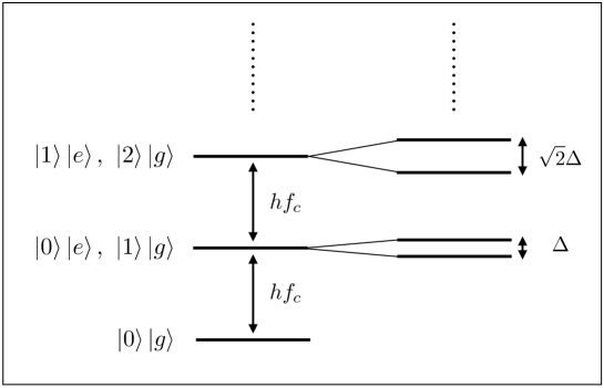
Figure 1: The diagonalized energy levels are depicted. The degenerated states, $\ket{n}\ket{e}$ and $\ket{n+1}\ket{g}$, are split by $\Delta\sqrt{n+1}$ due to the spin-orbit coupling.

V Detectability in electron $g$-factor measurements

In this section, we reveal how the general relativistic corrections investigated in the previous section appear in the observed $g$-factor (56) in Penning trap experiments. Furthermore, we estimate magnitude of the corrections and discuss its detectability in a concrete case of the electron $g$-factor measurement Hanneke et al. (2008).

As is discussed in the appendix A, the observed $g$-factor in Penning trap experiments is Eq. (56). On the other hand, we revealed the general relativistic corrections on the cyclotron and the Larmor frequencies in the previous sections, from Eqs. (42), (45) and (52), that is

$$\bar{f}_{c} =f_{c}\left(1+a_{i}x_{cy}^{i}\pm\frac{2\omega}{2\pi f_{c}}\cos\theta-\frac{1}{4\sqrt{2}}\frac{a}{\sqrt{(2\pi f_{c})m}}+\frac{GM/x_{0}^{3}}{(2\pi f_{c})^{2}}\right)\ ,$$ (53)

$$\bar{f}_{s} =f_{s}\left(1+a_{i}x_{cy}^{i}\pm\frac{\omega}{2\pi f_{s}}\cos\theta+\frac{1}{4\sqrt{2}}\frac{a}{\sqrt{(2\pi f_{c})m}}\right)\ .$$ (54)

From the above equations, general relativistic corrections on the observed $g$-factor can be read:

$$\frac{\delta g}{2} = \frac{\bar{f}_{s}}{\bar{f}_{c}}-\frac{f_{s}}{f_{c}}$$ (55)

$$\simeq \mp\frac{\omega}{2\pi f_{c}}\cos\theta+\frac{1}{2\sqrt{2}}\frac{a}{\sqrt{(2\pi f_{c})m}}-\frac{GM/x_{0}^{3}}{(2\pi f_{c})^{2}}\ .$$

One can find that the second terms in the right-hand side of Eqs. (53) and (54) canceled out. Each term in Eq. (55) has different dependence on $f_{c}$ and $m$. Therefore, their magnitude change depending on situations.

We now estimate the magnitude of the general relativistic corrections in Eq. (55), in particular for Hanneke et al. (2008). The experiment was conducted in Harvard University whose longitude is $42.4^{\circ}$. Thus, the angle between the Earth’s rotation vector $\bm{\omega}$ and the magnetic field $\bm{B}$ which is assumed to be perpendicular to the surface of the Earth would be $\theta\simeq 0.674\,{\rm rad}$. Furthermore, using values, $\omega=7.27\times 10^{-5}\,{\rm rad/s}$, $a=9.81\,{\rm m/s}^{2}$, $G=6.67\times 10^{-11}\,{\rm m^{3}/kg\,s^{2}}$, $M=5.97\times 10^{24}\,{\rm kg}$, $x_{0}=6.38\times 10^{6}\,{\rm m}$, $m=511\,{\rm keV}$ and $f_{c}=f_{s}=eB/m\simeq 150\,{\rm GHz}$ (see Hanneke et al. (2008)), we can estimate each correction. The result is summarized in Table 1. From Table 1, we see that the correction from the tidal effect is much smaller than other effects of inertial ones as expected. It should be mentioned that the correction from the the gravity of Earth, $\bm{a}$, is much larger than the previous report Ulbricht et al. (2019) where effects of $\bm{a}$ on the electron $g$-factor was studied. It is because that they investigated a correction from non linear contribution of $\bm{a}$ but did not focus on the spin-orbit coupling induced by $\bm{a}$, which is linear order contribution. Table 1 shows that the effects of Earth’s rotation cause the most largest correction to the electron $g$-factor in the case of Hanneke et al. (2008). It can be detected if the current uncertainty $\Delta g/2\simeq 2.8\times 10^{-13}$ Hanneke et al. (2008) is improved by 4 orders of magnitude. Therefore it would be important to consider the effects of gravity for future more accurate experiments Gabrielse et al. (2019); Fan et al. (2020).

Table 1: The general relativistic corrections in Eq. (55) for the case of the electron $g$-factor measurement Hanneke et al. (2008) are listed.

VI Conclusion

Electron $g$-factor measurements have been operated with remarkable high accuracy Hanneke et al. (2008); Odom et al. (2006); Van Dyck et al. (1987). Effects of gravity may not be negligible at the current sensitivity, so that quantitative and comprehensive study of general relativistic corrections in $g$-factor measurements is desired. In the first part of this paper, we revealed all linear order inertial and gravitational effects on a Dirac particle up to the order of $1/m$ in a proper reference frame, which is represented by the Hamiltonian (32). The Hamiltonian (32) is useful to investigate gravitational and inertial effects on any systems consistent with approximations we have made as it partly has been done for the case of a Hydrogen atom Parker (1980a, b); Perche and Neuser (2020). In the later part of this paper, we applied the Hamiltonian (32) to Penning trap experiments where a Dirac particle experiences the cyclotron motion and the spin precession in a cavity, i.e., a geonium atom, and evaluated the magnitude of the effects of gravity.

It turned out that gravity modifies the cyclotron motion and the spin precession in various ways. These effects were investigated in the section IV in details. Importantly, each general relativistic correction has different dependence on the cyclotron frequency $f_{c}=eB/m$ and the mass $m$. Therefore, the magnitude of each contribution can differ in situations.

In the section V, we considered an electron $g$-factor measurement and estimated the magnitude of each correction. The result is summarized in Table 1. The most largest correction comes from the effects of the rotation of the Earth and it can be detected if the current sensitivity is improved by 4 orders of magnitude. Therefore it would be important to consider the effects of gravity for future more accurate experiments Gabrielse et al. (2019); Fan et al. (2020).

Finally, we mention that our discussion can be applied to cases for $g$-factor measurements of positron Gabrielse et al. (2019); Van Dyck et al. (1987); Schwinberg et al. (1981), the proton Rodegheri et al. (2012); DiSciacca and Gabrielse (2012) and the antiproton DiSciacca et al. (2013); Gabrielse et al. (1999) in parallel. It is explicitly shown in Eq. (55) that the proton and the antiproton (the electron and the positron) should take the minus (plus) sign. For the case of the muon Abi et al. (2021); Bennett et al. (2006); Bailey et al. (1979), we need a more careful consideration because the velocity of the muon is in special relativistic regime. In the present paper, we have focused on general relativistic effects that are leading order with respect to $v/c$ and neglected higher order terms. Therefore, the accuracy of the approximation would be worse if we apply the discussion to the case of the muon. However, of course, since $v/c<1$ is satisfied even for the case of the muon, our result still would be valid to estimate magnitude of general relativistic corrections in the muon $g$-factor measurements. For instense, we can evaluate the correction from the Earth’s rotation to the muon $g$-factor measurement conducted at the Fermi National Accelerator Laboratory Abi et al. (2021) as $\delta g/2\sim 1.2\times 10^{-12}$, which coincides with the estimation in Notari and Bertacca (2019). Compared with the electron case, the correction is relatively colose to the current uncertainty of the muon $g$-factor measurement $\Delta g/2\sim 5.4\times 10^{-10}$ Abi et al. (2021). Therefore, it may also be detectable in the near future.

Appendix A Brief review of Penning trap experiments

In this appendix, we give an overview of Penning trap experiments and identify an observable in electron $g$-factor measurements. More detailed discussions would be found in Brown and Gabrielse (1986); D’Urso (2003); Hanneke et al. (2011).

First of all, to measure the electron $g$-factor, we apply an external magnetic field on an electron. Then, the electron experiences the cyclotron motion and the spin precession with the cyclotron frequency, $2\pi f_{c}=\frac{eB}{m}$, and the Larmor frequency, $2\pi f_{{s}}=\frac{g}{2}\frac{eB}{m}$, respectively. Therefore, $g/2$ can be observed by measuring the above frequencies or the anomaly frequency defined by $f_{a}=f_{s}-f_{c}$:

$$\frac{g}{2}=\frac{f_{s}}{f_{c}}=1+\frac{f_{a}}{f_{c}}\ .$$ (56)

In turn, let us consider a more realistic situation for measurements. In the experiment Hanneke et al. (2008), an electron is confined in a Penning trap cavity where an electrostatic quadrupole potential $V=V_{0}\frac{z^{2}-(x^{2}+y^{2})}{2d^{2}}$ is present in addition to an external magnetic field $B=(0,0,B)$. Then, the electron oscillates along with the $z$-direction at an axial frequency, $2\pi f_{z}=\sqrt{\frac{eV_{0}}{md^{2}}}$. The projected motion into $x$-$y$ plane traces an epicyclic orbit, which consists of a slow rotation with a large radius at a magnetron frequency, $f_{m}=\frac{f_{c}-\sqrt{f_{c}^{2}-2f_{z}^{2}}}{2}$, and a fast rotation with a small radius at a modified cyclotron frequency,

$$f_{c}^{\prime}=\frac{f_{c}+\sqrt{f_{c}^{2}-2f_{z}^{2}}}{2}=f_{c}-f_{m}\ .$$ (57)

Thus, using a modified anomaly frequency $f_{a}^{\prime}=f_{s}-f_{c}^{\prime}$, Eq. (56) is rewritten as

$$\frac{g}{2}=1+\frac{f_{a}^{\prime}-f_{z}^{2}/2f_{c}^{\prime}}{f_{c}^{\prime}+f_{z}^{2}/2f_{c}^{\prime}}\ ,$$ (58)

where we have used $f_{m}=f_{z}^{2}/2f_{c}^{\prime}$. Note that we have omitted a shift of $f_{c}^{\prime}$ due to special relativistic corrections and coupling with cavity modes Brown and Gabrielse (1986); Hanneke et al. (2008, 2011) because they are not relevant for our purpose. One can see that the $g$-factor is determined by measuring $f_{c}^{\prime}$, $f_{a}^{\prime}$ and $f_{z}$. Indeed, in Hanneke et al. (2008), above frequencies were measured directly or indirectly. The relation among $f_{c}^{\prime}$, $f_{s}$ and $f_{a}^{\prime}$ is illustrated in Fig. 2. We can determine the frequencies by measuring radiated photons from energy transitions among the energy levels. However, typically, the modified cyclotron frequency is $f_{c}^{\prime}\sim 100$ GHz, the modified anomaly frequency is $f_{a}^{\prime}\sim 100$ MHz and the axial frequency is $f_{z}\sim 100$ MHz. Determining energies of radiated photons with high accuracy around $\sim 100$ GHz is difficult. Then we are led to operation of quantum jump spectroscopy by monitoring $f_{z}$, which is measured continuously by detecting current induced by the axial motion.

In order to operate the quantum jump spectroscopy, we additionally apply a weak magnetic bottle field $B\propto z^{2}$ in the cavity. Then, the axial motion interacts with the cyclotron motion and the spin precession through the bottle field. It results in a shift of the axial frequency $f_{z}$ depending on the quantum numbers of the cyclotron and the spin energy levels. Importantly, the interaction Hamiltonian commutes with the cyclotron and the spin Hamiltonian, so that a quantum nondemolition measurement of the cyclotron and the spin states is allowed through monitoring $f_{z}$. Actually in the measurement Hanneke et al. (2008), deriving fields corresponding to $f_{c}^{\prime}$ and $f_{a}^{\prime}$ are applied in the cavity and then $f_{c}^{\prime}$ and $f_{a}^{\prime}$ can be determined by monitoring time variation of $f_{z}$ due to the cyclotron and the anomaly energy transition. This quantum jump spectroscopy enables us to determine the $g$-factor with very high accuracy. Remarkably, the current accuracy reaches $2.8\times 10^{-13}$ Hanneke et al. (2008).

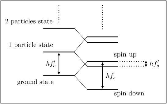
Figure 2: The relation of the energy states associated with $f_{c}^{\prime}$, $f_{s}$ and $f_{a}^{\prime}$ is illustrated. The left side ladders represent the energy states of the cyclotron motion. They are split into the spin up and the spin down states.

References

- Aoyama et al. (2019) T. Aoyama, T. Kinoshita, and M. Nio, Atoms 7, 28 (2019).
- Aoyama et al. (2020) T. Aoyama et al., (2020), 10.1016/j.physrep.2020.07.006, arXiv:2006.04822 [hep-ph] .
- Giudice et al. (2012) G. Giudice, P. Paradisi, and M. Passera, JHEP 11, 113 (2012), arXiv:1208.6583 [hep-ph] .
- Czarnecki and Marciano (2001) A. Czarnecki and W. J. Marciano, Phys. Rev. D 64, 013014 (2001), arXiv:hep-ph/0102122 .
- Hanneke et al. (2008) D. Hanneke, S. Fogwell, and G. Gabrielse, Phys. Rev. Lett. 100, 120801 (2008), arXiv:0801.1134 [physics.atom-ph] .
- Odom et al. (2006) B. C. Odom, D. Hanneke, B. D’Urso, and G. Gabrielse, Phys. Rev. Lett. 97, 030801 (2006).
- Van Dyck et al. (1987) R. Van Dyck, P. Schwinberg, and H. Dehmelt, Phys. Rev. Lett. 59, 26 (1987).
- Abi et al. (2021) B. Abi et al. (Muon g-2), Phys. Rev. Lett. 126, 141801 (2021), arXiv:2104.03281 [hep-ex] .
- Bennett et al. (2006) G. Bennett et al. (Muon g-2), Phys. Rev. D 73, 072003 (2006), arXiv:hep-ex/0602035 .
- Bailey et al. (1979) J. Bailey et al. (CERN-Mainz-Daresbury), Nucl. Phys. B 150, 1 (1979).
- Brown and Gabrielse (1986) L. S. Brown and G. Gabrielse, Rev. Mod. Phys. 58, 233 (1986).
- D’Urso (2003) B. R. D’Urso, Cooling and self - excitation of a one - electron oscillator, Other thesis (2003).
- Hanneke et al. (2011) D. Hanneke, S. Hoogerheide, and G. Gabrielse, Phys. Rev. A 83, 052122 (2011), arXiv:1009.4831 [physics.atom-ph] .
- Morishima et al. (2018) T. Morishima, T. Futamase, and H. M. Shimizu, PTEP 2018, 089201 (2018), arXiv:1801.10244 [hep-ph] .
- Visser (2018) M. Visser, (2018), arXiv:1802.00651 [hep-ph] .
- Nikolic (2018) H. Nikolic, (2018), arXiv:1802.04025 [hep-ph] .
- Venhoek (2018) D. Venhoek, (2018), arXiv:1804.09524 [hep-ph] .
- László and Zimborás (2018) A. László and Z. Zimborás, Class. Quant. Grav. 35, 175003 (2018), arXiv:1803.01395 [gr-qc] .
- Jentschura (2018) U. D. Jentschura, Phys. Rev. A 98, 032508 (2018), arXiv:1808.02089 [hep-ph] .
- Ulbricht et al. (2019) S. Ulbricht, R. A. Müller, and A. Surzhykov, Phys. Rev. D 100, 064029 (2019), arXiv:1907.01460 [gr-qc] .
- Ni and Zimmermann (1978) W.-T. Ni and M. Zimmermann, Phys. Rev. D 17, 1473 (1978).
- Ito and Soda (2020) A. Ito and J. Soda, Eur. Phys. J. C 80, 545 (2020), arXiv:2004.04646 [gr-qc] .
- Notari and Bertacca (2019) A. Notari and D. Bertacca, JHEP 11, 030 (2019), arXiv:1905.03649 [hep-ph] .
- Foldy and Wouthuysen (1950) L. L. Foldy and S. A. Wouthuysen, Phys. Rev. 78, 29 (1950).
- Bjorken and Drell (1965) J. D. Bjorken and S. D. Drell, (1965).
- Birrell and Davies (1984) N. D. Birrell and P. C. W. Davies, Quantum Fields in Curved Space, Cambridge Monographs on Mathematical Physics (Cambridge Univ. Press, Cambridge, UK, 1984).
- Huang and Parker (2009) X. Huang and L. Parker, Phys. Rev. D 79, 024020 (2009), arXiv:0811.2296 [hep-th] .
- Parker (1980a) L. Parker, Phys. Rev. Lett. 44, 1559 (1980a).
- Parker (1980b) L. Parker, Phys. Rev. D 22, 1922 (1980b).
- Perche and Neuser (2020) T. R. Perche and J. Neuser, (2020), [This paper appeared after submission of our paper.], arXiv:2012.08539 [gr-qc] .
- Gneiting et al. (2013) C. Gneiting, T. Fischer, and K. Hornberger, Phys. Rev. A 88, 062117 (2013), arXiv:1309.5017 [quant-ph] .
- Singh and Papini (2000) D. Singh and G. Papini, Nuovo Cim. B 115, 223 (2000), arXiv:gr-qc/0007032 .
- Werner et al. (1979) S. Werner, J. Staudenmann, and R. Colella, Phys. Rev. Lett. 42, 1103 (1979).
- Mashhoon (1988) B. Mashhoon, Phys. Rev. Lett. 61, 2639 (1988).
- Hehl and Ni (1990) F. W. Hehl and W.-T. Ni, Phys. Rev. D 42, 2045 (1990).
- Jaynes and Cummings (1963) E. T. Jaynes and F. W. Cummings, Proceedings of the IEEE 51, 89 (1963).
- Gabrielse et al. (2019) G. Gabrielse, S. Fayer, T. Myers, and X. Fan, Atoms 7, 45 (2019), arXiv:1904.06174 [quant-ph] .
- Fan et al. (2020) X. Fan, S. Fayer, T. Myers, B. Sukra, G. Nahal, and G. Gabrielse, (2020), arXiv:2011.08136 [quant-ph] .
- Schwinberg et al. (1981) P. Schwinberg, R. Van Dyck, and H. Dehmelt, Phys. Rev. Lett. 47, 1679 (1981).
- Rodegheri et al. (2012) C. Rodegheri, K. Blaum, H. Kracke, S. Kreim, A. Mooser, W. Quint, S. Ulmer, and J. Walz (BASE), New J. Phys. 14, 063011 (2012).
- DiSciacca and Gabrielse (2012) J. DiSciacca and G. Gabrielse, Phys. Rev. Lett. 108, 153001 (2012), arXiv:1201.3038 [physics.atom-ph] .
- DiSciacca et al. (2013) J. DiSciacca et al. (ATRAP), Phys. Rev. Lett. 110, 130801 (2013), arXiv:1301.6310 [physics.atom-ph] .
- Gabrielse et al. (1999) G. Gabrielse, A. Khabbaz, D. Hall, C. Heimann, H. Kalinowsky, and W. Jhe, Phys. Rev. Lett. 82, 3198 (1999).