Level sets of depth measures and central dispersion in abstract spaces

Abstract

The lens depth of a point has been recently extended to general metric spaces, which is not the case for most depths. It is defined as the probability of being included in the intersection of two random balls centred at two random points $X$ and $Y$, with the same radius $d(X,Y)$. We study the consistency in Hausdorff and measure distance, of the level sets of the empirical lens depth, based on an iid sample on a general metric space. We also prove that the boundary of the empirical level sets are consistent estimators of their population counterparts, and analyze two real-life examples.

1 Introduction

Statistical depth functions have gained importance in the last three decades. The best well-known and most studied among them include the half space depth [1], the simplicial depth [2, 3], and the multivariate $L^{1}$ depth.

Other well-known depths are the convex hull peeling depth [4], the Oja depth [5], and the spherical depth [6], among others. They have been extended to functional spaces, see [7, 8, 9, 10], to Riemannian manifolds, see [11], and also to general metric spaces, see [12]. Several different applications of depths notions have been proposed, in particular for classification problems, by means of the depth-depth method [13], or to functional data, see [14]. Most classical notions of depth, introduced initially on $\mathbb{R}^{d}$, can not be directly extended to general metric spaces or even to functional spaces or manifolds. Some of them are computationally infeasible on high dimensional spaces, such as Liu’s or Tukey’s depth, because the computational complexity is exponential in the number of dimensions. This is not the case of the depth introduced in [15], i.e. the lens depth, whose computational complexity is of order $n^{2}$, and, as we will see, it can be easily extended to general metric spaces. This makes the lens depth particularly suitable for estimating it’s level sets, by means of the level sets of it’s empirical version, based on an iid sample, which is one of the main goals of this manuscript. An extension to Riemannian manifolds of the lens depth (called weighed lens depth) was recently introduced in [16] to tackle the supervised classification problem, and a point-wise a.s consistency result is obtained (see Theorem 2). Here we focus on a different problem, i.e: level set estimation of the lens depth on general metric spaces. This require uniform a.s. consistency of the empirical lens depth to the population one, which is developed in Section 3.

Level set estimation of depths was initially studied in [1], as a key tool for the visualization and exploration of data. Other significant contributions can be found in [17, 18, 19, 20]). As it was pointed out in [21], “the shape and size of these levels, as well as the direction and speed at which they expand, provides insight into the dispersion, kurtosis, and asymmetry of the underlying distribution”. It also allows to extend the notion of quantiles to multivariate or functional data, and can be used for outlier detection, see for instance [22, 23], as well as for supervised classification, see [24, 25].

More formally, let $X_{1},X_{2}$ be two random variables defined on a (rich enough) probability space $(\Omega,\mathcal{A},\mathbb{P})$, taking values in a complete separable metric space $(M,d)$ endowed with the Borel $\sigma$-algebra. Assume that they are independent and identically distributed. In what follows, the distribution of a random element $X$ of $M$ will be denoted by $P_{X}$.

Given $x_{1},x_{2}\in M$ define their “associate lens” by

$$A(x_{1},x_{2}):=B(x_{1},d(x_{1},x_{2}))\cap B(x_{2},d(x_{1},x_{2})),$$

where $B(p,r)$ is the closed ball centred at $p$ with radius $r>0$. The lens depth of a point $x\in M$ is defined by $\textrm{LD}(x)=\mathbb{P}(x\in A(X_{1},X_{2}))$. Given an iid sample $\mathcal{X}_{n}=\{X_{1},\ldots,X_{n}\}$ from a distribution $P_{X}$, the empirical version of LD is given by the $U$-statistics of order two,

$$\widehat{\textrm{LD}}_{n}(x)=\binom{n}{2}^{-1}\sum_{1\leq i_{1}<i_{2}\leq n}\mathbbm{1}_{A(X_{i_{1}},X_{i_{2}})}(x).$$ (1)

To gain some insight into the shape of $\{\widehat{\textrm{LD}}_{n}\geq\lambda\}$, see Figure 1.

The general approach to obtain consistency results (w.r.t. Hausdorff distance) for the plug-in estimator $\{\widehat{\textrm{LD}}_{n}\geq\lambda\}$ to its population counterpart $\{\textrm{LD}\geq\lambda\}$ is to prove the uniform convergence of $\widehat{\textrm{LD}}_{n}$ to LD.

In general metric spaces it will be necessary to restrict the convergence to compact sets. This is proved in Theorem 4, but the results also hold on $\mathbb{R}^{d}$ under milder conditions, see Theorem 5.

This paper is organized as follows. Section 2 introduces the notation, some previous definitions, and states two important results given in Theorems 1 and 2 that will be used to prove our main results. The almost surely (a.s.) uniform consistency of $\widehat{\textrm{LD}}_{n}$ is stated in Section 3, while its asymptotic distribution is formulated in Section 4. The a.s. consistency in Hausdorff and measure distance, for the empirical level sets $\{\widehat{\textrm{LD}}_{n}\geq\lambda\}$, as well as the a.s. consistency of its boundary, is stated in Section 5. Lastly, in Section 6 we tackle the study of two interesting real datasets, the vectocardiogram dataset (see subsection 6.1) and the influenza dataset (see subsection 6.2). All proofs are given in the Appendix.

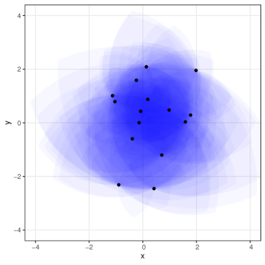
(a)

Figure 1: Level sets of the lens depth based on a sample of 15 iid random vectors, distributed as a bivariate standard normal distribution. The intensity of blue represents the depth.

2 Preliminaries

In this section we will introduce the notation and necessary definitions used throughout this paper. Given a metric space $(M,d)$, which will be assumed to be separable, complete and locally connected, we denote by $B(x,r)$ the closed ball centred at $x$ with radius $r>0$. The boundary of a set $A\subset M$ is denoted by $\partial M$. Given $x\in A^{c}$, $d(x,A)=\inf_{a\in A}d(x,a)$ and $\textrm{diam}(A)=\sup_{x,y\in A}d(x,y)$. Given two closed sets $A,B$, the Hausdorff distance between them is defined as

$$d_{H}(A,B)\mathrel{\mathop{:}}=\max\Big{\{}\max_{a\in A}d(a,B),\ \max_{b\in B}d(b,A)\Big{\}}$$ (2)

Given a function $f:M\rightarrow\mathbb{R}$ and $\lambda\in\mathbb{R}$, we denote by $\{f\geq\lambda\}$ the $\lambda$-level set $\{x\in M:f(x)\geq\lambda\}$.

For the estimation of level sets in general metric spaces, two main results will play a key role. The first one is Theorem 2.1 in [26]. We will make use of the following slightly restricted version.

Theorem 1 (Molchanov, (1998)).

Let $f_{n},f:M\to\mathbb{R}$ be continuous functions. Assume that for each compact set $K_{0}$, $\sup_{x\in K_{0}}|f_{n}(x)-f(x)|\to 0$. Assume that for all $\lambda\in[c_{1},c_{2}]$, $\{f\geq\lambda\}\subset\overline{\{f>\lambda\}}$. Then

$$\sup_{c_{1}\leq\lambda\leq c_{2}}d_{H}\big{(}\{f_{n}\geq\lambda\}\cap K_{0},\{f\geq\lambda\}\cap K_{0}\big{)}\to 0.$$

The convergence of the boundaries of the level sets is in general more involved. To prove that, we will use the following result.

Theorem 2 (Cuevas, Gozález-Manteiga, Rodríguez-Casal, (2006)).

Given a continuous function $f:M\to\mathbb{R}$, let $(\Omega,\mathcal{A},P)$ be a probability space and $f_{n}=f_{n}(\omega,\cdot)$, with $\omega\in\Omega$, a sequence of random functions, $f_{n}:M\to\mathbb{R}$, $n=1,2,\dots,$. Assume that for each $n$, $f_{n}$ is continuous with probability one. Assume that the following assumptions are fulfilled.

• $M$ is locally connected.

• For all $x\in\partial\{f\geq\lambda\}$, there exist sequences $u_{n},l_{n}\to x$ such that $f(u_{n})>\lambda$ and $f(l_{n})<\lambda$.

• $\partial\{f\geq\lambda\}\neq\emptyset$. Moreover, there exists a $\lambda^{-}<\lambda$ such that the set $\{f\geq\lambda^{-}\}$ is compact.

If $\sup_{x\in M}\big{|}f(x)-f_{n}(x)\big{|}\rightarrow 0$ a.s., then

$$d_{H}\big{(}\partial\{f\geq\lambda\},\partial\{f_{n}\geq\lambda\}\big{)}\to 0,\quad a.s.,\textrm{ as }n\rightarrow\infty.$$

3 Uniform consistency of $\widehat{\textrm{LD}}_{n}$

As mentioned above, the key points to prove the consistency in Hausdorff distance of the level sets of $\widehat{\textrm{LD}}_{n}$ are Theorems 2 and 1. Then we have to prove that $\widehat{\textrm{LD}}_{n}$ converges uniformly to LD a.s., which is the main goal of this section.

To obtain the a.s. uniform convergence of $\widehat{\textrm{LD}}_{n}$, we will use the following version of Theorem 1 in [27].

Theorem 3 (Billingsley and Topsøe, (1967)).

Let $\mathcal{B}(M\times M)$ be the class of all real valued, bounded, measurable functions defined on the metric space $(M\times M,\rho)$, where $\rho(z,y)=\max\{d(z_{1},y_{1}),d(z_{2},y_{2})\}$. Suppose $\mathcal{F}\subset\mathcal{B}(M\times M)$ is a subclass of functions. Then

$$\sup_{f\in\mathcal{F}}\Big{|}\int fdP_{n}-\int fdP\Big{|}\rightarrow 0,$$

for every sequence $P_{n}$ that converges weakly to $P$ if, and only if,

$$\sup\{|f(z)-f(t)|:f\in\mathcal{F},z=(z_{1},z_{2}),t=(t_{1},t_{2})\in M\times M\}<\infty,$$

and for all $\epsilon>0$,

$$\lim_{\delta\rightarrow 0}\sup_{f\in\mathcal{F}}P\Big{[}\{y=(y_{1},y_{2}):\omega_{f}\{B_{\rho}(y,\delta)\}\geq\epsilon\}\Big{]}=0,$$ (3)

where $\omega_{f}(A)=\sup\{|f(z)-f(t)|:z,t\in A\}$ and $B_{\rho}(y,\delta)$ is the open ball in the metric space $(M\times M,\rho)$ of radius $\delta>0$.

To prove that (3) is fulfilled, we will use the following lemma.

Lemma 1.

Let $x\in M$ and $y=(y_{1},y_{2})\in M\times M$ be such that $d(x,\partial A(y_{1},y_{2}))>3\delta$. Then $\omega_{f_{x}}\{B_{\rho}(y,\delta)\}=0$, where $f_{x}(t_{1},t_{2})=\mathbb{I}_{A(t_{1},t_{2})}(x)$ with $t_{1},t_{2}\in M$.

Theorem 4.

Let $(M,d)$ be a complete separable metric space and $P_{X}$ a Borel measure on $M$. Assume that $P_{X}(\partial B(x,\delta))=0$ for all $x\in M$ and $\delta>0$. For any compact set $K\subset M$,

$$\sup_{x\in K}|\widehat{\textrm{LD}}_{n}(x)-\textrm{LD}(x)|\to 0\quad a.s.,\text{ as }n\to\infty.$$

As a direct consequence of the previous results, if $M$ is a compact manifold, we have that $\sup_{x\in M}|\widehat{\textrm{LD}}_{n}(x)-\textrm{LD}(x)|\to 0$. For $\mathbb{R}^{d}$, uniform convergence can be obtained, as stated in the following theorem.

Theorem 5.

Assume that $P_{X}(\partial B(x,\delta))=0$ for all $x\in\mathbb{R}^{d}$ and $\delta>0$. Then

$$\sup_{x\in\mathbb{R}^{d}}|\widehat{\textrm{LD}}_{n}(x)-\textrm{LD}(x)|\to 0\quad a.s.,\text{ as }n\to\infty.$$

4 Asymptotic distribution

To obtain the asymptotic law of $\widehat{\textrm{LD}}_{n}$ we will use Proposition 10 of [28], which is a very general result for empirical processes, applied to $U$ statistics. This requires proving that the family of sets $\{A(x,y),x,y\in M\}$ has finite Vapnik–Chervonenkis (VC) dimension (see [29]). To prove the result, we introduce the Vapnik-ball condition.

Definition 1.

A metric space $(M,d)$ fulfills Vapnik-ball condition if the the family $\{F_{p}\}_{p\in M}$ where $F_{p}=\{(x,y)\in M\times M:d(p,x)<d(x,y)\}$ has finite VC dimension varying $p$.

Let us introduce some notation and general ideas of empirical processes, following [30]. To each $x\in M$ we associate the function $f_{x}:M^{2}\to\mathbb{R}$ defined by $f_{x}(a,b)=\mathbb{I}_{A(a,b)}(x)$. The family of all these functions is denoted by $\mathcal{F}$. Then we can define $\widehat{\textrm{LD}}_{n}$, a function of the random variable $X$ and the point $x$, by

$$\widehat{\textrm{{LD}}}_{n}(P_{X},f_{x})=\binom{n}{2}^{-1}\sum_{1\leq i<j\leq n}f_{x}(X_{i},X_{j}),$$

where $X_{1},\dots,X_{n}$ is an iid sample from $X$ with distribution $P_{X}$. Denote the metric space of all real valued bounded functions defined on $\mathcal{F}$, endowed with the supremum norm, by $l^{\infty}(\mathcal{F})$. We can consider $\widehat{\textrm{LD}}_{n}$ as a random variable with values in $l^{\infty}(\mathcal{F})$ given by $\omega\in\Omega\to\widehat{\textrm{LD}}_{n}:\mathcal{F}\to\mathbb{R}$. We define $\textrm{LD}\in l^{\infty}(\mathcal{F})$ by $\textrm{LD}(f_{x})=\mathbb{P}(f_{x}(X_{1},X_{2}))$, with $X_{1},X_{2}$ being independent copies of $X$. We want to derive the limit law of the random element of $l^{\infty}(\mathcal{F})$ given by $G_{n}=\sqrt{n}(\widehat{\textrm{LD}}_{n}-\textrm{LD})$. The limit law of $G_{n}$ is denoted by $2GP_{X}$, where $GP_{X}$ is a Brownian bridge associated to $P_{X}$, which is a random element in $l^{\infty}(\mathcal{F})$, and is defined through its finite dimensional distributions. More precisely, for all $k$, $(GP_{X}(f_{x_{1}}),\dots,GP_{X}(f_{x_{k}}))$ is a zero-mean Gaussian process whose $k\times k$ covariance matrix has $(i,j)$th element

$$E(GP_{X}(f_{x_{i}})GP_{X}(f_{x_{j}}))=P_{2}(f_{x_{i}}f_{x_{j}})-P_{2}(f_{x_{i}})P_{2}(f_{x_{j}}),$$ (4)

where

$$P_{2}(f_{x})\mathrel{\mathop{:}}=\int_{M^{2}}f_{x}(x_{1},x_{2})dP_{X}(x_{1})\times dP_{X}(x_{2}).$$

The convergence of $G_{n}$ to $2GP_{X}$ is in law, which in this case is equivalent to the convergence in distribution of the random vector $(G_{n}(f_{x_{1}}),\dots,G_{n}(f_{x_{k}}))$ to $N(0,\Sigma)$, where the $k\times k$ matrix $\Sigma$ has $(i,j)$th element given by (4).

Theorem 6.

(Limit Law) Let $M$ be a compact manifold fulfilling the Vapnik-ball condition. Following the previous notation, the stochastic processes $G_{n}$ converge in law to $2GP_{X}$, as $n\to\infty$.

5 Level set estimation

Given positive numbers $c_{1}<c_{2}$, assume that for all $\lambda\in[c_{1},c_{2}]$, we have $\{f\geq\lambda\}\subset\overline{\{f>\lambda\}}$. From Theorem 2.1 in [26] together with Theorem 4, and the fact that LD is a continuous function, we get

$$\sup_{c_{1}\leq\lambda\leq c_{2}}d_{H}\big{(}\{\widehat{\textrm{LD}}_{n}\geq\lambda\}\cap K,\{\textrm{LD}\geq\lambda\}\cap K\big{)}\to 0\quad a.s.,\text{ as }\quad n\to\infty$$

for any compact set $K$. If $\nu(\{\textrm{LD}=\lambda\})=0$, it follows easily from Theorem 4 that for all compact $K$,

$$d_{\nu}\big{(}\{\widehat{\textrm{LD}}_{n}\geq\lambda\}\cap K,\{\textrm{LD}\geq\lambda\}\cap K\big{)}\to 0\quad a.s.,\text{ as }\quad n\to\infty.$$

The following theorem states that $\partial\{\widehat{\textrm{LD}}_{n}\geq\lambda\}\cap K$ is a consistent estimator of $\partial\{\textrm{LD}\geq\lambda\}\cap K$. The proof follows the same lines used to prove Theorem 1 in [31]. However, we can not apply that theorem directly because $\widehat{\textrm{LD}}_{n}(x)$ is not a continuous function, since the range of $\widehat{\textrm{LD}}_{n}(x)$ is contained in the set $\{k\binom{n}{2}^{-1}:k=0,\dots,\binom{n}{2}\}$.

Theorem 7.

Let $\lambda>0$ be such that $\{\textrm{LD}\geq\lambda\}\neq\emptyset$. Under the assumptions of Theorem 4, together with hypotheses $h1$ and $h2$ of Theorem 2, we have that

$$\lim_{n\to\infty}d_{H}\big{(}\partial\{\widehat{\textrm{LD}}_{n}\geq\lambda\}\cap K,\partial\{\textrm{LD}\geq\lambda\}\cap K\big{)}=0\quad a.s.,$$

for all compact sets $K$.

For the metric space $(\mathbb{R}^{d},\|\cdot\|)$ endowed with the Euclidean norm we have the following trivial corollary,

Corollary 1.

Assume that hypothesis h2 of Theorem 2 is fulfilled. Assume also that $\{\textrm{LD}\geq\lambda^{-}\}$ is non-empty and compact, for some $\lambda^{-}<\lambda$. Then

$$\lim_{n\to\infty}d_{H}(\partial\{\widehat{\textrm{LD}}_{n}\geq\lambda\},\partial\{\textrm{LD}\geq\lambda\})=0\quad a.s.$$ (5)

6 An application to the study of two sets of real data

In what follows we analize two interesting real data sets: the vectocardiogram and the influenza data sets.

6.1 The vectocardiogram dataset

We consider a real life dataset, where the data belong to the Stiefel manifold $SO(3,2)$ of all orthonormal $2$-frames in $\mathbb{R}^{3}$ considered as $3\times 2$ orthogonal matrices (see [32]). The dataset consists of 98 vectocardiograms from children with ages varying between 2 and 19. Vectocardiography is a method that produces a three dimensional curve which comprises the records of the magnitude and direction of the electrical forces generated by the heart over time. These curves are called QRS loops, see Figure 2. In [33] there is associated to each curve an element of $SO(3,2)$ that represents some of the information of the curve, see also [34].

This sample has been previously analysed in the literature, see for instance [35, 36, 37]. A very important problem is outlier detection, corresponding to children with (possibly) cardiological problems.

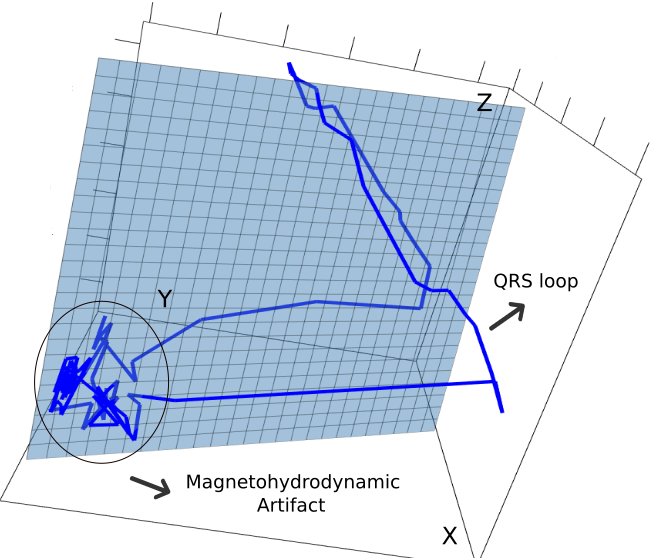
(a)

Figure 2: QRS curve loop. The plane in blue is the best two dimensional approximation of the curve by least squares.

Figure 3 represents each matrix in $SO(3,2)$ as two points in $S^{2}$, one for each column. They are joined by an arc in $S^{2}$. The arc joining the deepest pair of observations (w.r.t. lens depth) is represented in violet, while the outliers (for a level $\lambda=0.10$) are represented as red arcs.

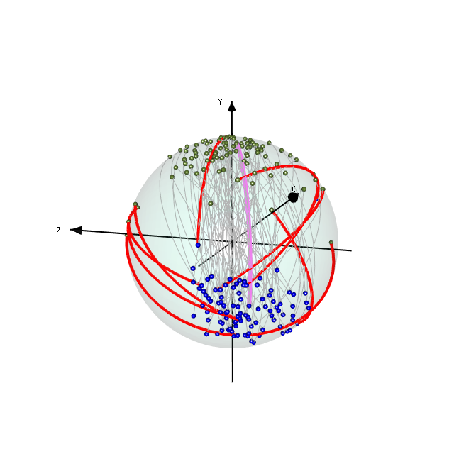
(a)

Figure 3: Data visualization of the data from $SO(3,2)$. The violet arc represents the deepest observation according to lens depth. The outliers represented by red arcs correspond to the data outside the $\lambda=0.10$ level set of the depth.

6.2 Influenza dataset

This dataset consists of longitudinal data of the influenza virus, belonging to the family Orthomyxoviridae. An important problem analized in [12], is to model the genomic evolution of the virus, see [38]. In this paper we focus on another important issue: modelling the temporal variability of the virus by means of the lens depth, and use this to predict and anticipate a possible pandemic. The influenza virus has an RNA genomic which is very common: it produces diseases like yellow fever and hepatitis and annually costs half a million deaths worldwide. It is well known that these viruses change their genetic pattern over time, which is vital for developing a possible vaccine. We will study the the H3N2 variant of the virus, in particular, the subtype hemagglutini (HA), which produced the SARS pandemic in 2002. This variant is known to have a variability in its genetic arrangement over time, see [39, 40].

The dataset can be found in GI-SAID $\textrm{EpiFlu}^{TM}$ database , providing 1089 genomic sequences of H3N1 from 1993 to 2017 in New York, aligned using MUSCULE, see [41]. We used reduced trees of 5 leaves, as in [40], to capture the structure of the data. This set of trees can be endowed with a distance, see [42]. The database used was obtained from the GitHub repository https://github.com/antheamonod/FluPCA.

For this kind of data, constructing measures of centrality and variability, as well as confidence regions, is a problem that has been previously addressed in the literature, see for instance [43, 44, 45] and references therein.

For each year we computed the empirical lens depth of the trees, considered on the manifold of phylogenetic trees. We estimated the diameter of the level sets from the sample points that belong to the level sets, see Figure 4. As can be seen, there is a larger dispersion in the years prior to the pandemic of 2002 compared to later years.

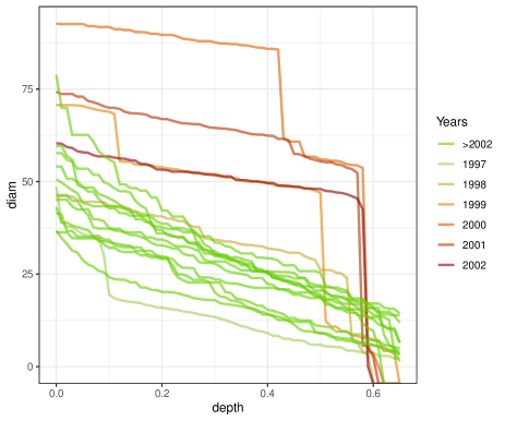
(a)

Figure 4: Diameters of the lens depth level sets from the sample of trees for the different years, with respect to $\lambda$.

Appendix

Proof of Lemma 1

If $z=(z_{1},z_{2})\in B_{\rho}(y,\delta)$, then $d(z_{1},y_{1})<\delta$ and $d(z_{2},y_{2})<\delta$. Let us prove first that

$$\{x\in A(y_{1},y_{2}):d(x,\partial A(y_{1},y_{2}))>2\delta\}\subset A(z_{1},z_{2})$$ (6)

for all $z=(z_{1},z_{2})\in B_{\rho}(y,\delta)$. If $x\in A(y_{1},y_{2})$ and $d(x,\partial A(y_{1},y_{2}))>2\delta$, then $d(x,y_{1})\leq d(y_{1},y_{2})-2\delta\leq d(y_{1},z_{1})+d(z_{1},z_{2})+d(z_{2},y_{2})-2\delta\leq d(z_{1},z_{2})$. In the same way, if $d(x,y_{2})\leq d(z_{1},z_{2})$, then $x\in A(z_{1},z_{2})$, which implies (6). Next let us prove that

$$A(z_{1},z_{2})\subset\{x:d(x,A(y_{1},y_{2}))\leq 3\delta\}$$ (7)

For any $x\in A(z_{1},z_{2})$, $d(x,y_{1})\leq d(x,z_{1})+d(z_{1},y_{1})\leq d(z_{1},z_{2})+\delta\leq d(y_{1},y_{2})+3\delta$. In the same way, $d(x,y_{2})\leq d(x,z_{2})+\delta\leq d(z_{1},z_{2})+\delta\leq d(y_{1},y_{2})+3\delta$. Then $x\in\{x:d(x,A(y_{1},y_{2}))\leq 3\delta\}$. To prove that $\omega_{f_{x}}\{B_{\rho}(y,\delta)\}=0$, it is enough to prove that for all $(z_{1},z_{2}),(t_{1},t_{2})\in B_{\rho}((y_{1},y_{2}),\delta)$

$$|\mathbb{I}_{A(z_{1},z_{2})}(x)-\mathbb{I}_{A(t_{1},t_{2})}(x)|=0.$$ (8)

Observe that if $x\in A(y_{1},y_{2})$ and $d(x,\partial A(y_{1},y_{2}))>3\delta$, then by (6), $x\in A(z_{1},z_{2})$, so $\mathbb{I}_{A(z_{1},z_{2})}(x)=0$ and $x\in A(t_{1},t_{2})$ and hence $\mathbb{I}_{A(t_{1},t_{2})}(x)=0$ which then shows that (8) holds. Proceeding in the same way if $x\notin A(y_{1},y_{2})$ and $d(x,\partial A)>3\delta$, by (7) $x\notin A(z_{1},z_{2})$, which implies that $\mathbb{I}_{A(z_{1},z_{2})}(x)=0$. Also $x\notin A(t_{1},t_{2})$, which implies that $\mathbb{I}_{A(t_{1},t_{2})}(x)=0$, so again (8) holds. $\square$

Proof of Theorem 4

We will apply Billingsley’s theorem to the set of functions

$$\mathcal{F}=\{f_{x}(z,y)=\mathbb{I}_{A(z,y)}(x):x\in K\},$$

where the sequence $P_{n}$ of probability measures on $M\times M$ is such that $P_{n}(X_{i},X_{j})=(1/2)\binom{n}{2}^{-1}$ if $i\neq j$ and $P_{n}(X_{i},X_{j})=0$ if $i=j$. Let $P$ be the product measure $P_{X}\times P_{X}$. In this case

$$\sup_{f\in\mathcal{F}}\Big{|}\int fdP_{n}-\int fdP\Big{|}=\sup_{x\in K}|\widehat{\textrm{LD}}_{n}(x)-\textrm{LD}(x)|.$$

Clearly, $\sup\{|f(z)-f(t)|:f\in\mathcal{F},z,t\in M\times M\}=2$. So we have to prove that (3) holds. By Lemma (1), to prove (3), it is enough to prove that

$$\lim_{\delta\to 0}\sup_{x\in K}P_{X}\times P_{X}\{(y_{1},y_{2}):d(x,\partial A(y_{1},y_{2}))\leq 3\delta\}=0.$$

By the dominated convergence theorem, since $P_{X}(\partial B(x,\delta))=0$ for all $\delta>0$ and all $x\in M$, it follows that for fixed $\delta$, $P_{X}\times P_{X}\{(y_{1},y_{2}):d(x,\partial A(y_{1},y_{2}))\leq 3\delta\}$ is a continuous function of $x$. Also, for a fixed $x$, $P_{X}\times P_{X}\{(y_{1},y_{2}):d(x,\partial A(y_{1},y_{2}))\leq 3\delta\}\to 0$, again by the dominated convergence theorem.

By Lemma 1,

$$\sup_{x\in K}P_{X}\times P_{X}\Big{[}\{y=(y_{1},y_{2}):\omega_{f_{x}}\{B_{\rho}(y,\delta)\}\geq\epsilon\}\Big{]}\leq\\ \sup_{x\in K}P_{X}\times P_{X}\{(y_{1},y_{2}):d(x,\partial A(y_{1},y_{2}))\leq 3\delta\}$$

which converges to $0$ as $\delta\to 0$. $\square$

Proof of Theorem 5

Let $\epsilon>0$ and suppose that $R$ is large enough so that $P_{X}(\overline{B(0,R)}^{c})<\epsilon$, and take $K=\overline{B(0,R)}$. We will apply the previously mentioned theorems of Billingsley and Topsøe to the set of functions

$$\mathcal{F}=\{f_{x}(z,y)=\mathbb{I}_{A(z,y)}(x):x\in\mathbb{R}^{d}\}.$$

We start by splitting into two terms

$$\sup_{x}P_{X}\times P_{X}\Big{[}\{y=(y_{1},y_{2}):\omega_{f_{x}}\{B_{\rho}(y,\delta)\}\geq\epsilon\}\Big{]}\leq\\ \sup_{x\in K}P_{X}\times P_{X}\Big{[}\{y=(y_{1},y_{2}):\omega_{f_{x}}\{B_{\rho}(y,\delta)\}\geq\epsilon\}\Big{]}+\\ \sup_{x\in K^{c}}P_{X}\times P_{X}\Big{[}\{y=(y_{1},y_{2}):\omega_{f_{x}}\{B_{\rho}(y,\delta)\}\geq\epsilon\}\Big{]}=I_{1}+I_{2}.$$

By Lemma 1, $I_{1}\leq\sup_{x\in K}P_{X}\times P_{X}\{(y_{1},y_{2}):d(x,\partial A(y_{1},y_{2}))\leq 3\delta\},$ which converges to $0$ as $\delta\to 0$. Regarding $I_{2}$, we bound

$$P_{X}\times P_{X}\Big{[}\{y=(y_{1},y_{2}):\omega_{f_{x}}\{B_{\rho}(y,\delta)\}\geq\epsilon\}\Big{]}\leq\\ P_{X}\times P_{X}\Big{[}\{y=(y_{1},y_{2}):y_{1},y_{2}\in K\text{ and }\omega_{f_{x}}\{B_{\rho}(y,\delta)\}\geq\epsilon\}\Big{]}\\ +P_{X}\times P_{X}\Big{[}\{y=(y_{1},y_{2}):y_{1}\in K^{c}\text{ or }y_{2}\in K^{c}\text{ and }\omega_{f_{x}}\{B_{\rho}(y,\delta)\}\geq\epsilon\}\Big{]}.$$

The second term is bounded from above by $2P_{X}(K^{c})<2\epsilon$. Lastly, to tackle the first term, by Lemma 1, it only remains to prove that

$$\lim_{\delta\to 0}\sup_{x\in K^{c}}P_{X}\times P_{X}\Big{[}\{y=(y_{1},y_{2}):y_{1},y_{2}\in K\text{ and }d(x,\partial A(y_{1},y_{2}))<3\delta\Big{]}=0.$$

Lastly, let $\delta_{0}$ be small enough such that $P_{X}((\partial K)^{3\delta})<\epsilon$ for all $\delta<\delta_{0}$. If $y_{1},y_{2}\in B(0,R-3\delta)$, then $d(x,A(y_{1},y_{2}))\geq 3\delta$. Therefore,

$$P_{X}\times P_{X}\Big{[}\{y=(y_{1},y_{2}):y_{1},y_{2}\in K\text{ and }d(x,\partial A(y_{1},y_{2}))<3\delta\Big{]}\leq\\ P_{X}(y_{1}\in(\partial K)^{3\delta}\text{ or }y_{2}\in(\partial K)^{3\delta})<2\epsilon.$$ (9)

$\square$

Proof of Theorem 6
By assumption, we have that $\mathcal{F}$ has a finite $VC$-dimension. This implies that the assumptions in Proposition $10$ in [28] hold for an order $2$ $U$-statistic and the asymptotic distribution is derived from Theorem 4.10 in [30]. $\square$

Proof of Theorem 7

Let $K$ be any compact set. Observe that $\{\textrm{LD}\geq\lambda^{-}\}\cap K$ is nonempty and compact for any $0<\lambda^{-}<\lambda$. Following the same ideas as those used in the proof of Theorem 1 in [31], one can derive that for all $\epsilon>0$

$$\partial\{\textrm{LD}\geq\lambda\}\cap K\subset B(\partial\{\widehat{\textrm{LD}}_{n}\geq\lambda\}\cap K,\epsilon).$$

The proof of

$$\partial\{\widehat{\textrm{LD}}_{n}\geq\lambda\}\cap K\subset B(\partial\{\textrm{LD}\geq\lambda\}\cap K,\epsilon)$$

is slightly different from the analogous inclusion in [31]. If we proceed by contradiction, there exists an $x_{n}\in\{\widehat{\textrm{LD}}_{n}\geq\lambda\}\cap K$, but

$$d(x_{n},\partial\{\textrm{LD}\geq\lambda\}\cap K)>\epsilon.$$ (10)

Observe that if $x_{n}\in\partial\{\widehat{\textrm{LD}}_{n}\geq\lambda\}\cap K$, then $x_{n}\in\partial A(X_{i},X_{j})$ for some $X_{i}\neq X_{j}$. If $x_{n}$ is in the boundary of two or more sets $A(X_{i},X_{j})$, we can take $y_{n}$ such that $d(y_{n},x_{n})<\epsilon/2^{n}$, $y_{n}\in\partial\{\widehat{\textrm{LD}}_{n}(x)\geq\lambda\}$, $y_{n}$ in the boundary of only one $\partial A(X_{i},X_{j})$ and $|\widehat{\textrm{LD}}_{n}(y_{n})-\lambda|<\binom{n}{2}^{-1}$. If $x_{n}$ is in the boundary of only one $A(X_{i},X_{j})$, we choose $x_{n}=y_{n}$. In this case we clearly have also have $|\widehat{\textrm{LD}}_{n}(y_{n})-\lambda|<\binom{n}{2}^{-1}$

Since $K$ is compact, there exists an $x\in K$ such that $x_{n},y_{n}\to x$ (by considering a subsequence if necessary). Then $|\textrm{LD}(x)-\lambda|\leq|\textrm{LD}(x)-\textrm{LD}(y_{n})|+|\textrm{LD}(y_{n})-\widehat{\textrm{LD}}(y_{n})|+|\widehat{\textrm{LD}}(y_{n})-\lambda|$. The first terms converge to $0$ by the continuity of LD at $x$. The second term converges to $0$ a.s., because the set $K^{\prime}=\{\cup_{n}\{y_{n}\}\}\cup\{x\}$ is compact and by Theorem 4, $\sup_{z\in K^{\prime}}|\widehat{\textrm{LD}}_{n}(z)-\textrm{LD}(z)|\to 0$. The last term is bounded from above by $\binom{n}{2}^{-1}\to 0$ as $n\to\infty$. Then $\textrm{LD}(x)=\lambda$, which implies that $d(x_{n},\partial\{\textrm{LD}\geq\lambda\}\cap K)\leq d(x_{n},x)\to 0$, which contradicts (10). $\square$

References

- [1] J. W. Tukey, Mathematics and the picturing of data, in: Proceedings of the international congress of mathematicians, Vol. 2, 1975, pp. 523–531.
- [2] R. Y. Liu, On a Notion of Data Depth Based on Random Simplices, The Annals of Statistics 18 (1) (1990) 405–414.
- [3] R. Y. Liu, Data depth and multivariate rank tests, L1-statistical analysis and related methods (Y. Dodge, ed.) (1992) 279–294.
-
[4]
V. Barnett, The ordering of
multivariate data, Journal of the Royal Statistical Society. Series A
(General) 139 (3) (1976) 318–355.
URL http://www.jstor.org/stable/2344839 - [5] H. Oja, Descriptive statistics for multivariate distributions, Statistics & Probability Letters 1 (6) (1983) 327–332.
- [6] R. T. Elmore, T. P. Hettmansperger, F. Xuan, Spherical data depth and a multivariate median, DIMACS Series in Discrete Mathematics and Theoretical Computer Science 72 (2006) 87.
- [7] R. Fraiman, G. Muniz, Trimmed means for functional data, Test 10 (2) (2001) 419–440.
- [8] S. López-Pintado, J. Romo, On the concept of depth for functional data, Journal of the American Statistical Association 104 (486) (2009) 718–734.
- [9] G. Claeskens, M. Hubert, L. Slaets, K. Vakili, Multivariate functional halfspace depth, Journal of the American Statistical Association 109 (505) (2014) 411–423.
- [10] A. Cuevas, R. Fraiman, On depth measures and dual statistics. a methodology for dealing with general data, Journal of Multivariate Analysis 100 (4) (2009) 753–766.
- [11] R. Fraiman, F. Gamboa, L. Moreno, Connecting pairwise geodesic spheres by depth: Dcops, Journal of Multivariate Analysis 169 (2019) 81–94.
- [12] R. Fraiman, F. Gamboa, L. Moreno, Weighted lens depth: Some applications to supervised classification, arcXiv (2020).
- [13] O. Vencálek, Depth-based classification for multivariate data, Austrian Journal of Statistics 46 (3-4) (2017) 117–128.
- [14] K. Mosler, P. Mozharovskyi, Fast dd-classification of functional data, Statistical Papers 58 (4) (2017) 1055–1089.
- [15] Z. Liu, R. Modarres, Lens data depth and median, Journal of Nonparametric Statistics 23 (4) (2011) 1063–1074.
- [16] A. Cholaquidis, R. Fraiman, L. Moreno, Level set and density estimation on manifolds, arXiv (2020).
- [17] G. Koshevoy, K. Mosler, et al., Zonoid trimming for multivariate distributions, Annals of Statistics 25 (5) (1997) 1998–2017.
- [18] Y. Zuo, R. Serfling, General notions of statistical depth function, The Annals of Statistics 28 (2) (2000) 461–482.
- [19] R. Serfling, Quantile functions for multivariate analysis: approaches and applications, Statistica Neerlandica 56 (2) (2002) 214–232.
- [20] R. Dyckerhoff, Convergence of depths and depth-trimmed regions, arXiv preprint arXiv:1611.08721 (2016).
- [21] R. Y. Liu, J. M. Parelius, K. Singh, et al., Multivariate analysis by data depth: descriptive statistics, graphics and inference,(with discussion and a rejoinder by liu and singh), The annals of statistics 27 (3) (1999) 783–858.
- [22] M. Febrero, P. Galeano, W. González-Manteiga, Outlier detection in functional data by depth measures, with application to identify abnormal nox levels, Environmetrics: The official journal of the International Environmetrics Society 19 (4) (2008) 331–345.
- [23] W. Dai, M. G. Genton, Directional outlyingness for multivariate functional data, Computational Statistics and Data Analysis 131 (2019) 50 – 65.
- [24] I. Ruts, P. J. Rousseeuw, Computing depth contours of bivariate point clouds, Computational Statistics and Data Analysis 23 (1) (1996) 153 – 168.
- [25] M. Hubert, P. Rousseeuw, P. Segaert, Multivariate and functional classification using depth and distance, Advances in Data Analysis and Classification 11 (3) (2017) 445–466.
- [26] I. S. Molchanov, A limit theorem for solutions of inequalities, Scandinavian Journal of Statistics 25 (1) (1998) 235–242.
- [27] P. Billingsley, F. Topsøe, Uniformity in weak convergence, Zeitschrift für Wahrscheinlichkeitstheorie und verwandte Gebiete 7 (1) (1967) 1–16.
- [28] E. Giné, Empirical processes and applications: an overview, Bernoulli 2 (1) (1996) 1–28.
- [29] L. Devroye, L. Györfi, G. Lugosi, A probabilistic theory of pattern recognition, Vol. 31, Springer Science & Business Media, 2013.
-
[30]
M. A. Arcones, E. Gine, Limit
theorems for u–processes, The Annals of Probability 21 (3) (1993)
1494–1542.
URL http://www.jstor.org/stable/2244585 - [31] A. Cuevas, W. González-Manteiga, A. Rodríguez-Casal, Plug-in estimation of general level sets, Australian & New Zealand Journal of Statistics 48 (1) (2006) 7–19.
- [32] A. Hatcher, Algebraic topology, 2005.
- [33] T. D. Downs, J. Liebman, Statistical methods for vectorcardiographic directions, IEEE Transactions on Biomedical Engineering 1 (1969) 87–94.
- [34] T. D. Downs, Orientation statistics, Biometrika 59 (3) (1972) 665–676.
- [35] Y. Chikuse, Statistics on special manifolds, Vol. 174, Springer Science & Business Media, 2012.
- [36] R. Chakraborty, B. C. Vemuri, et al., Statistics on the stiefel manifold: theory and applications, The Annals of Statistics 47 (1) (2019) 415–438.
- [37] S. Pal, S. Sengupta, R. Mitra, A. Banerjee, A bayesian approach for analyzing data on the stiefel manifold, arXiv preprint arXiv:1907.04303 (2019).
- [38] D. J. Smith, A. S. Lapedes, J. C. de Jong, T. M. Bestebroer, G. F. Rimmelzwaan, A. D. Osterhaus, R. A. Fouchier, Mapping the antigenic and genetic evolution of influenza virus, science 305 (5682) (2004) 371–376.
- [39] L. K. Altman, This season’s flu virus is resistant to 2 standard drugs, New York Times (2006).
- [40] A. Monod, B. Lin, R. Yoshida, Q. Kang, Tropical geometry of phylogenetic tree space: A statistical perspective, arXiv preprint arXiv:1805.12400 (2018).
- [41] R. C. Edgar, Muscle: multiple sequence alignment with high accuracy and high throughput, Nucleic acids research 32 (5) (2004) 1792–1797.
- [42] L. J. Billera, S. P. Holmes, K. Vogtmann, Geometry of the space of phylogenetic trees, Advances in Applied Mathematics 27 (4) (2001) 733–767.
- [43] D. Barden, H. Le, M. Owen, Limiting behaviour of fréchet means in the space of phylogenetic trees, Annals of the Institute of Statistical Mathematics 70 (1) (2018) 99–129.
- [44] D. G. Brown, M. Owen, Mean and variance of phylogenetic trees, Systematic Biology 69 (1) (2020) 139–154.
- [45] A. Willis, Confidence sets for phylogenetic trees, Journal of the American Statistical Association 114 (525) (2019) 235–244.