Spectral shift via “lateral” perturbation

Abstract.

We consider a compact perturbation $H_{0}=S+K_{0}^{*}K_{0}$ of a self-adjoint operator $S$ with an eigenvalue $\lambda^{\circ}$ below its essential spectrum and the corresponding eigenfunction $f$. The perturbation is assumed to be “along” the eigenfunction $f$, namely $K_{0}f=0$. The eigenvalue $\lambda^{\circ}$ belongs to the spectra of both $H_{0}$ and $S$. Let $S$ have $\sigma$ more eigenvalues below $\lambda^{\circ}$ than $H_{0}$; $\sigma$ is known as the spectral shift at $\lambda^{\circ}$.

We now allow the perturbation to vary in a suitable operator space and study the continuation of the eigenvalue $\lambda^{\circ}$ in the spectrum of $H(K)=S+K^{*}K$. We show that the eigenvalue as a function of $K$ has a critical point at $K=K_{0}$ and the Morse index of this critical point is the spectral shift $\sigma$. A version of this theorem also holds for some non-positive perturbations.

Introduction

The first step in the proofs of several spectral geometry theorems is perturbing the operator “along” a given eigenfunction $f$. To give a classical example, the Courant bound on the number of nodal domains of the $n$-th eigenfunction $f=f_{n}$ of a Dirichlet Laplacian is shown by introducing additional Dirichlet conditions along the zero set of $f$. The function $f$ is still an eigenfunction of the perturbed operator and, as a consequence, the corresponding eigenvalue $\lambda$ remains in the spectrum.

Recently, it was discovered that some nodal properties of eigenfunctions are related to stability with respect to perturbation of the original operator of suitably defined energy functionals. More precisely, the nodal deficiency of the $n$-th eigenfunction $f_{n}$ on a manifold (defined as $n$ minus the number of the nodal domains of $f_{n}$) is equal to the Morse index of the energy of the nodal partition with respect to variation of the partition boundaries [BKS12]. On graphs, the nodal surplus (defined as the number of zeros of $f_{n}$ minus $n-1$) is equal to the Morse index of $\lambda_{n}$ considered as a function of the perturbation of the Schrödinger operator by the magnetic field [Ber13, CdV13, BW14]. One is left wondering what other types of perturbations can produce similar results. The answer is presented in this paper. Essentially this is true for any “sufficiently rich” family of perturbations.

At this point, we set up notation and outline terms and conditions. Let ${\mathcal{H}}$ be a separable Hilbert space with the inner product $\langle\cdot,\cdot\rangle$ (assumed linear with respect to the second argument) and $S:{\mathcal{H}}\to{\mathcal{H}}$ be a self-adjoint operator bounded from below. Assume that below its essential spectrum, $S$ has an eigenvalue $\lambda^{\circ}$ with the eigenfunction $f$. Consider further a self-adjoint non-negative perturbation operator $P$ such that $Pf=0$. This is a perturbation “along” the eigenfunction $f$: $f$ is also an eigenfunction of the perturbed operator $H:=S+P$ with eigenvalue $\lambda^{\circ}$. Assume that $\lambda^{\circ}$ is simple in the spectrum of $S+P$. If $\lambda^{\circ}$ has index $n$ in the spectrum of $H$, i.e. $\lambda^{\circ}=\lambda_{n}(S+P_{0})$ then, due to positivity of $P_{0}$, $\lambda^{\circ}=\lambda_{n+\sigma}(S)$ with some integer $\sigma\geq 0$. We call this value $\sigma$ the spectral shift. In the special case when $P_{0}$ has rank $r<\infty$, one has $0\leq\sigma\leq r$.

We remark that, in the hindsight, the theorems about nodal surplus or deficiency mentioned above are in fact statements about the spectral shift followed by some known relation between the index of the eigenvalue and the nodal count for the perturbed operator $H$. The spectral shift $\sigma$ and its relations to Morse indices is the primary object of interest here.

We now represent $P$ as a product $P=K_{0}^{*}K_{0}$, where $K_{0}$ is a compact operator from ${\mathcal{H}}$ to an auxiliary Hilbert space ${\mathcal{K}}$ and $K_{0}f=0$. We now allow the operator $K_{0}$ to vary, and consider the continuation of the eigenvalue $\lambda^{\circ}$ as a function of $K$. Namely, we consider $\Lambda(K):=\lambda(A+K^{*}K)$ such that $\Lambda(K_{0})=\lambda^{\circ}$. Due to the standard perturbation theory, this function is (real-)analytic with respect to $K$. We will prove that $\Lambda(K)$ has a critical point at $K=K_{0}$ and, if the family of variations $K$ is “rich enough,” the Morse index of this critical point is equal to the spectral shift $\sigma$. Here the Morse index is the number of negative eigenvalues of the Hessian at the critical point of the function.

By “rich enough” we mean the following. Perturbations by operators annihilating $f$ preserve $f$ as eigenfunction and do not affect the eigenvalue. We are interested in further (“lateral”) perturbations, which do change the eigenvalue and carry information about the spectral shift. To capture the entirety of this information (in the form of the Morse index), the family of variations has to be transversal to the subspace of operators $K$ such that $Kf=0$.

This result is important for a variety of extremal eigenvalue problems. For example, the question of optimizing an eigenvalue with respect to the location of a given perturbation has direct relevance to many applications, such as, for instance, photonic crystals (where one is interested in impurity modes in spectral gaps, to confine photons in cavities), or civil engineering (where the perturbation could be the introduction of extra supports in a beam structure, and the first eigenvalue is proportional to the critical pressure at which the structure will start to buckle). As mentioned above, our result also provides a unifying framework for the nodal counting theorems. In this manuscript we derive and strengthen one of them as an example. Finally, the classical tool of spectral theory, the Birman–Schwinger operator (or Schur complement in linear algebra), arises naturally as the Hessian with respect to variation of the perturbation. Its eigenfunctions are interpreted as giving the directions in which the eigenvalue changes the most.

1. Main results in the simplified form

Let ${\mathcal{H}}$ and ${\mathcal{K}}$ be separable complex Hilbert spaces and denote by ${\mathcal{C}}:={\mathcal{C}}({\mathcal{H}},{\mathcal{K}})$ the Banach space of compact linear operators from ${\mathcal{H}}$ to ${\mathcal{K}}$.

Let $\lambda^{\circ}$ be an eigenvalue of a bounded below self-adjoint operator $S:{\mathcal{H}}\to{\mathcal{H}}$, lying below the essential spectrum of $S$; let $f$ be the corresponding eigenfunction. Consider the perturbed operator $S+K_{0}^{*}K_{0}$, $K_{0}\in{\mathcal{C}}$ and assume $K_{0}f=0$ so that $\lambda^{\circ}$ is also an eigenvalue of $S+K_{0}^{*}K_{0}$. For a self-adjoint operator $A$ we denote by $N(\lambda^{\circ};A)$ the number of eigenvalues of $A$ below $\lambda^{\circ}$ and denote by $\sigma$ the spectral shift

$$\sigma=N(\lambda^{\circ};S)-N(\lambda^{\circ};S+K_{0}^{*}K_{0}).$$

We will now allow the perturbation $K_{0}$ to vary in the most general way, considering $H(K)=S+K^{*}K$ with $K$ ranging over an open neighborhood of $K_{0}$ in ${\mathcal{C}}$.

Denote by $F$ the subspace of ${\mathcal{C}}$ consisting of the rank one operators acting as $x\mapsto\langle f,x\rangle_{\mathcal{H}}\psi$, where $\psi\in{\mathcal{K}}$. The subspace $F$ is isometric to ${\mathcal{K}}$ and we have the direct decomposition ${\mathcal{C}}=F\oplus F^{\circ}$, where $F^{\circ}$ is the subspace of operators $K\in{\mathcal{C}}$ vanishing on $f$, i.e. such that $Kf=0$.

Here is a somewhat simplified version of the main result:

Theorem 1.1 (Main Theorem — a simplified form).

Let $\lambda^{\circ}$ be a simple eigenvalue of $S$ with eigenfunction $f$ and let $K_{0}f=0$. Consider the family

$$H(K)=S+K^{*}K,\qquad K\in{\mathcal{C}}({\mathcal{H}},{\mathcal{K}}).$$ (1)

Assume that the eigenvalue $\lambda^{\circ}$ is also simple in the spectrum of $H(K_{0})$ and let the function $\Lambda(K):=\lambda(H(K))$ be its real analytic continuation defined in a neighborhood of $K_{0}$ in ${\mathcal{C}}$. Then

1. $K=K_{0}$ is a critical point of the function $\Lambda(K)$,

2. the Hessian of $\Lambda(K)$ at $K=K_{0}$ is zero on the space $F^{\circ}$ and is reduced by the decomposition ${\mathcal{C}}=F\oplus F^{\circ}$,

3. the Hessian restricted to $F$ is a quadratic form on $F$ and its Morse index (number of its negative eigenvalues) is equal to the spectral shift $\sigma$.

By a “critical point” we mean that the $\mathbb{R}$-linear terms in the analytic expansion of $\Lambda(K)$ at $K=K_{0}$ are zero. By the “Hessian” we mean the quadratic terms of the real analytic expansion of $\Lambda(K)$. The theorem above directly follows from a more general result, Theorem 3.5 in Section 3, where we drop such restrictions as the simplicity of $\lambda^{\circ}$ in the spectrum of $S$ and $H(K)$ being a positive perturbation of $S$.

It is also not necessary to vary $K$ in all possible directions to recover the spectral shift as the Morse index of $\Lambda(K)$. Restricting $K$ to a submanifold in ${\mathcal{C}}$ transversal to $F^{\circ}$ we will obtain the same result in Theorems 3.10 and 3.11.

2. Morse indices and Schur complements

2.1. Morse indices

We define first the indices that are involved in our main results. We denote by $\sigma(H)$ the spectrum of $H$ and by $\sigma_{\mathrm{ess}}(H)$ its essential spectrum, defined as the complement of the set of $\lambda\in\mathbb{C}$ such that $H-\lambda$ is Fredholm. We recall that for self-adjoint operators, $\sigma(H)$ is the disjoint union of $\sigma_{\mathrm{ess}}(H)$ and the discrete spectrum $\sigma_{d}(H)$, i.e. the set of isolated eigenvalues of finite multiplicity.

Definition 2.1.

Let $H$ be a self-adjoint operator on ${\mathcal{H}}$. For an interval $I\subset\mathbb{R}$, we denote by $E_{I}$ the (projector-valued) spectral measure of $I$ corresponding to $H$. We define two indices $i_{-}$ and $i_{0}$ (which may be infinite) as follows:

$$i_{-}: =\dim\operatorname{Ran}E_{(-\infty,0)},$$ (2)

$$i_{0}: =\dim\operatorname{Ker}H,$$ (3)

where $\operatorname{Ker}$ denotes the kernel of the operator and $\operatorname{Ran}$ denotes the range.

We will refer to $i_{-}$ as the Morse index and to $i_{0}$ as the nullity of $H$.

A well-known and very useful equivalent formula for $i_{-}$ (often called Glazman’s lemma, see e.g. [BS91, Lemma 3.1 in Supplement 1]) looks as follows.

Lemma 2.2.

The Morse index $i_{-}$ is the maximal dimension of a subspace ${\mathcal{M}}$ on which operator $H$ is negative, i.e. $(x,Hx)<0$ for all $x\in{\mathcal{M}}$, $x\neq 0$.

This interpretation of the Morse index allows for a simple, general, and surely well known proof of the classical Sylvester’s law of inertia:

Lemma 2.3.

Let $H$ be a self-adjoint operator on ${\mathcal{H}}$ with domain $\operatorname{Dom}(H)$. If $S$ is a bounded invertible operator in ${\mathcal{H}}$, then $S^{*}HS$ is self-adjoint on the natural domain $S^{-1}(\operatorname{Dom}(H))$ and and

$$i_{-}(H) =i_{-}(S^{*}HS),$$ (4)

$$i_{0}(H) =i_{0}(S^{*}HS).$$ (5)

Proof.

Since $(x,S^{*}HSx)=(Sx,HSx)$ on $S^{-1}(\operatorname{Dom}(H))$, the operator $S^{-1}$ establishes an isomorphism between subspaces in $\operatorname{Dom}(H)$ and $\operatorname{Dom}(S^{*}HS)$, which preserves the negativity property (and in fact, the numerical range). ∎

2.2. Schur complement; finite dimensional case

We recall first the notion of the Schur complement in the matrix case. Let

$$M=\left(\begin{array}[]{cc}A&B\\ C&D\\ \end{array}\right)$$ (6)

be a block-matrix, with the diagonal block $D$ being invertible.

Definition 2.4.

The matrix $A-BD^{-1}C$ is called the Schur complement of $D$ in $M$ (or just Schur complement, if no confusion can arise). We denote it as follows:

$$M/D:=A-BD^{-1}C$$ (7)

The name (introduced by E. Haynsworth [Hay68]) comes from a well known J. Schur determinant formula [Sch17], which was based on a Gauss elimination procedure reducing $M$ to the form

$$\left(\begin{array}[]{cc}A-BD^{-1}C&B\\ 0&D\\ \end{array}\right).$$ (8)

2.3. Schur complement; unbounded operators

Let operator $H$ be as in the beginning of the section, and $P_{1}$ be an orthogonal projector keeping the domain $\operatorname{Dom}(H)$ invariant, i.e. $P_{1}\operatorname{Dom}(H)\subset\operatorname{Dom}(H)$. We denote by ${\mathcal{H}}_{1}$ and ${\mathcal{H}}_{2}$ the ranges of projector $P_{1}$ and of the complementary projector $P_{2}:=I-P_{1}$ respectively. We thus have the orthogonal decomposition

$${\mathcal{H}}={\mathcal{H}}_{1}\dot{\oplus}{\mathcal{H}}_{2}.$$ (9)

Thus, operator $H$ can be represented in the block form

$$H=\begin{pmatrix}A&B\\ \widetilde{B}&D\end{pmatrix},$$ (10)

where all blocks are closed operators between the corresponding spaces. Due to self-adjointness of $H$, it checks out that $A$ and $D$ are self-adjoint in the spaces ${\mathcal{H}}_{1}$ and ${\mathcal{H}}_{2}$ correspondingly with the natural domains $P_{i}(\operatorname{Dom}(H))$. Also, the operator $\widetilde{B}:{\mathcal{H}}_{1}\to{\mathcal{H}}_{2}$ is adjoint to $B:{\mathcal{H}}_{2}\to{\mathcal{H}}_{1}$. We thus end up with the decomposition

$$H=\begin{pmatrix}A&B\\ B^{*}&D\end{pmatrix}.$$ (11)

A thorough study of operators represented in this form can be found in [Tre08].

We need to remind the reader the following notion:

Definition 2.5.

An operator $D^{+}$ is said to be a generalized inverse to $D$ if the following equality holds:

$$DD^{+}D=D.$$ (12)

In other words, $D^{+}$ is a right inverse to $D$ on the range of $D$.

Remark 2.6.

Different flavors of generalized inverses exist (see, for example, [BIG03, Chap. 9]), but the above basic property is sufficient for our purposes. The reader should notice that an operator $D^{+}$ satisfying (12) always exists, for example defined on $\operatorname{Ran}(D)$, without requiring $D$ to be injective or surjective. A particular choice, satisfying more restrictive conditions which guarantee uniqueness, is the Moore–Penrose (pseudo-)inverse.

The following formula, proved originally for matrices, goes back at least to a 1968 article by Haynsworth [Hay68].

Theorem 2.7.

Let $H$ be a self-adjoint operator on ${\mathcal{H}}$ and let ${\mathcal{H}}_{1}\dot{\oplus}{\mathcal{H}}_{2}={\mathcal{H}}$ be the orthogonal decomposition described above, in particular $P_{1}\operatorname{Dom}(H)\subset\operatorname{Dom}(H)$.

1. If $0\not\in\sigma_{\mathrm{ess}}(D)$ and for some constant $C>0$ and all $x\in{\mathcal{H}}_{2}$,

   $$\|Bx\|_{{\mathcal{H}}_{1}}\leq C\|Dx\|_{{\mathcal{H}}_{2}},$$ (13)

   then, with any choice $D^{+}$ of the generalized inverse of $D$, the operator $A-BD^{+}B^{*}$ is self-adjoint and

   $$i_{-}(H) =i_{-}(D)+i_{-}\left(A-BD^{+}B^{*}\right),$$ (14)

   $$i_{0}(H) =i_{0}(D)+i_{0}\left(A-BD^{+}B^{*}\right),$$ (15)

   assuming the relevant indices are finite.

2. If $0\not\in\sigma_{\mathrm{ess}}(A)\cup\sigma_{\mathrm{ess}}(D)$ and, in addition to (13),

   $$\|B^{*}x\|_{{\mathcal{H}}_{2}}\leq C\|Ax\|_{{\mathcal{H}}_{1}},$$ (16)

   for some $C>0$, one has

   $$i_{-}(A)-i_{-}(D)=i_{-}\left(A-BD^{+}B^{*}\right)-i_{-}\left(D-B^{*}A^{+}B\right),$$ (17)

   $$i_{0}(A)-i_{0}(D)=i_{0}\left(A-BD^{+}B^{*}\right)-i_{0}\left(D-B^{*}A^{+}B\right),$$ (18)

   assuming the relevant indices are finite.

Remark 2.8.

1. Equations (14) and (15) are known in the matrix case as the “Haynsworth formula”, usually formulated under the condition of invertibility of $D$. Extended version using various flavors of generalized matrix inverses are also known, see e.g. [CHM74, HF85, Mad88, JMRT87, Tia10] and [BCCM20, Thm A.1]. To the best of our knowledge, the present version might be the first one for unbounded operators with not necessarily invertible $D$ (however, several similar results are contained in [Tre08]). Extending Definition 2.4, we will call the operator $A-BD^{+}B^{*}$ the Schur complement $M/D$ of $D$ in $M$.

2. Condition (13) implies the inclusion $\operatorname{Ker}D\subset\operatorname{Ker}B$. In finite dimension, they are equivalent.

3. Part (1) of the theorem has a symmetric counterpart: if $0\not\in\sigma_{\mathrm{ess}}(A)$ and (13) is replaced with (16), one has

   $$i_{-}(H) =i_{-}(A)+i_{-}\left(D-B^{*}A^{+}B\right),$$ (19)

   $$i_{0}(H) =i_{0}(A)+i_{0}\left(D-B^{*}A^{+}B\right),$$ (20)

   assuming the relevant indices of $H$ and $A$ are finite. This is used, in particular, to prove part (2) of the theorem.

4. Part (2) of the theorem shows that the spectral shift between the operators $A$ and $D$ is the same as between their Schur complements. In particular, if indices of $A$ and $D$ coincide, then those of $M/A$ and $M/D$ also do.

5. According the Definition 2.1, we need 0 to be away from the essential spectrum of the corresponding operator in order to have the indices $i_{0}$ and $i_{-}$ well-defined. In particular, $i_{0}$ will be finite. But we need not assume finiteness of $i_{-}$ in order to use (15) or (18).

Our proof of Theorem 2.7 mostly adheres to the existing proofs for matrices, except for the use of Lemma 2.2 instead of the original definition of the indices. We prove the following auxiliary statement first.

Lemma 2.9.

Let $D$ be a self-adjoint operator on ${\mathcal{H}}_{2}$ and let $0\not\in\sigma_{\mathrm{ess}}(D)$. If condition (13) holds for an operator $B:{\mathcal{H}}_{2}\to{\mathcal{H}}_{1}$, then the following properties hold:

1. the operator $BD^{+}B^{*}$ does not depend on the choice of the generalized inverse $D^{+}$,

2. for an arbitrary choice of $D^{+}$, we have $BD^{+}D=B$,

3. there exists a self-adjoint choice of $D^{+}$, such that the operator $BD^{+}$ is bounded,

Proof.

Since zero is not in the essential spectrum of $D$, $D$ is Fredholm and its range $D$ is closed. From inequality (13) we have $\operatorname{Ker}D\subset\operatorname{Ker}B$ and therefore $\operatorname{Ran}B^{*}\subset\overline{\operatorname{Ran}D}=\operatorname{Ran}D$.

Let now $D^{+}$ be an arbitrary generalized inverse of $D$. Equation (12) implies that $D(D^{+}Dx-x)=0$ for any $x\in\operatorname{Dom}D$, or, equivalently

$$D^{+}Dx-x\in\operatorname{Ker}D\subset\operatorname{Ker}B.$$ (21)

We apply $B$ to (21) and obtain

$$BD^{+}Dx-Bx=0,$$ (22)

establishing part (2) of the lemma.

Since $\operatorname{Ran}B^{*}\subset\operatorname{Ran}D$, for a given $y$ there exists an $x\in\operatorname{Dom}D$ such that $B^{*}y=Dx$. Then (22) becomes $BD^{+}B^{*}y=Bx$ and, since $x$ did not depend on the choice of $D^{+}$, neither does the operator $BD^{+}B$.

Finally, let $P$ be the orthogonal projection onto the range of $D$, then $D$ restricted to the space $P{\mathcal{H}}_{1}=\operatorname{Ran}D$ is self-adjoint and has a bounded inverse, which we denote by $D_{P}^{-1}$. The generalized inverse $P^{+}=PD_{P}^{-1}P=D_{P}^{-1}\oplus 0$ is self-adjoint (the latter representation is with respect to the decomposition ${\mathcal{H}}_{1}=\operatorname{Ran}D\dot{\oplus}\operatorname{Ker}D$). Furthermore, (13) yields

$$\|BD^{+}x\|_{{\mathcal{H}}_{2}}\leq C\|DD^{+}x\|_{{\mathcal{H}}_{1}}=C\|Px\|_{{\mathcal{H}}_{1}}\leq C\|x\|_{{\mathcal{H}}_{1}},$$

establishing part (3). ∎

Proof of Theorem 2.7.

According to the lemma, it is enough to prove (14)-(15) for one particular choice of $D^{+}$ and we will use the self adjoint $D^{+}$ such that the operator $BD^{+}$ is bounded. This implies boundedness and invertibility of the operator matrix

$$Q:=\begin{pmatrix}I&BD^{+}\\ 0&I\end{pmatrix}.$$

We can now represent the operator matrix $H$ as follows:

$$H=\begin{pmatrix}A&B\\ B^{*}&D\end{pmatrix}=Q\begin{pmatrix}A-BD^{+}B^{*}&0\\ 0&D\end{pmatrix}Q^{*}.$$ (23)

Indeed, direct calculation shows

$$Q\begin{pmatrix}A-BD^{+}B^{*}&0\\ 0&D\end{pmatrix}Q^{*}=\begin{pmatrix}A-BD^{+}B^{*}+BD^{+}D(D^{+})^{*}B^{*}&BD^{+}D\\ D(D^{+})^{*}B^{*}&D\end{pmatrix},$$

and the identities $BD^{+}D=B$ and $(D^{+})^{*}=D^{+}$ do the rest.

From Sylvester’s law of inertia (Lemma 2.3), we have that $A-BD^{+}B^{*}$ is self-adjoint and

$$i_{-}\left(H\right)=i_{-}\left(\begin{pmatrix}A-BD^{+}B^{*}&0\\ 0&D\end{pmatrix}\right)=i_{-}(D)+i_{-}\left(A-BD^{+}B^{*}\right),$$ (24)

by definition 2.1 and the orthogonal decomposition of the spectral projectors of the block-diagonal operator matrix. The equality for $i_{0}$ is established in the same way.

To establish the second part of the theorem, we reverse the roles of $A$ and $D$ and (with estimate (16) playing the role of (13)) obtain

$$i_{-}(H) =i_{-}(A)+i_{-}\left(D-B^{*}A^{+}B\right),$$

$$i_{0}(H) =i_{0}(A)+i_{0}\left(D-B^{*}A^{+}B\right),$$

Using (14) and (15) to eliminate $i_{-}(H)$ and $i_{0}(H)$ we obtain the desired result. ∎

Remark 2.10.

The Schur complement technique (and its close relatives) is very natural and thus has been re-invented many times under various guises, e.g. as Dirichlet-to-Neumann operators, $m$-functions for ODEs, Birman–Schwinger approach, and probably many others.

3. The main result

Let ${\mathcal{H}}$ and ${\mathcal{K}}$ be separable complex Hilbert spaces and, as before, we denote by ${\mathcal{C}}({\mathcal{H}},{\mathcal{K}})$ the Banach space of compact operators from ${\mathcal{H}}$ to ${\mathcal{K}}$.

Definition 3.1.

We denote by $F$ the subspace of ${\mathcal{C}}({\mathcal{H}},{\mathcal{K}})$ consisting of the operators $K_{\psi}$ acting as

$$K_{\psi}:x\in{\mathcal{H}}\mapsto\langle f,x\rangle\psi,$$ (25)

for some $\psi\in{\mathcal{K}}$.

The subspace $F^{\circ}$ consists of operators $K$ such that $Kf=0$.

Remark 3.2.

Alternatively, $F$ can be defined as the subspace of $K\in{\mathcal{C}}({\mathcal{H}},{\mathcal{K}})$ such that $\operatorname{Ker}K\supset f^{\perp}:=\{u\in{\mathcal{H}}\colon\langle f,u\rangle=0\}$.

Lemma 3.3.

1. The correspondence $\psi\leftrightarrow K_{\psi}$ is an isometry between ${\mathcal{K}}$ and $F$.

2. $F\oplus F^{\circ}={\mathcal{C}}$.

Proof.

To compute the operator norm of $K_{\psi}$ we use Cauchy–Schwartz inequality, keeping in mind that $\|f\|=1$,

$$\|K_{\psi}x\|_{\mathcal{K}}=|\langle f,x\rangle|\|\psi\|_{\mathcal{K}}\leq\|\psi\|_{\mathcal{K}}\|x\|_{\mathcal{H}},$$

with equality achieved when $x=f$.

The splitting of a $K\in{\mathcal{C}}({\mathcal{H}},{\mathcal{K}})$ is given explicitly by

$$\langle f,\cdot\rangle Kf\in F\quad\mbox{and}\quad K-\langle f,\cdot\rangle Kf\in F^{\circ}.$$

∎

Let $H_{0}$ be a bounded below self-adjoint operator on ${\mathcal{H}}$ and $\lambda^{\circ}$ be its simple isolated eigenvalue with the corresponding normalized eigenfunction $f$. Assume that the spectrum of $H_{0}$ below $\lambda^{\circ}$ consists of finitely many eigenvalues of finite multiplicity. Suppose also that $H_{0}$ is of the form

$$H_{0}=S+K_{0}^{*}\Omega K_{0},\qquad\mbox{with}\quad K_{0}\in F^{\circ},\mbox{ i.e. }K_{0}f=0,$$ (26)

where $\Omega$ is a bounded invertible self-adjoint operator on ${\mathcal{K}}$, whose spectrum below zero consists of finitely many eigenvalues of finite multiplicity, so $i_{0}(\Omega)=0$ and $i_{-}(\Omega)<\infty$.

Since $K_{0}f=0$, $f$ is also an eigenfunction of $S$ with the same eigenvalue $\lambda^{\circ}$. The essential spectrum of $S$ also lies above $\lambda^{\circ}$, although $\lambda^{\circ}$ may no longer be simple in the spectrum of $S$.

Let, as before, $i_{-}(H_{0}-\lambda^{\circ})$ be the number of eigenvalues (counted with multiplicity) of $H_{0}$ below $\lambda^{\circ}$ and denote by $\sigma$ the spectral shift

$$\sigma:=\sigma(\lambda^{\circ};S,H_{0}):=i_{-}(S-\lambda^{\circ})-i_{-}(H_{0}-\lambda^{\circ}).$$ (27)

Remark 3.4.

Notice that when $\Omega$ is positive, the spectral shift is also positive.

Consider the family of operators

$$H(K)=S+K^{*}\Omega K,\qquad K\in{\mathcal{C}}({\mathcal{H}},{\mathcal{K}}),$$ (28)

so, in particular, $H(K_{0})=H_{0}$.

Since $\lambda^{\circ}$ is a simple eigenvalue of $H_{0}=H(K_{0})$, there is a real-analytic branch $\Lambda(K)$ of the eigenvalues of $H(K)$ that is the continuation of $\lambda^{\circ}$ defined to a neighborhood $\Pi$ of $K_{0}$ in ${\mathcal{C}}({\mathcal{H}},{\mathcal{K}})$. Real analyticity means, in particular, the existence of the expansion

$$\Lambda(K)=\lambda_{0}+A_{1}(\delta\!K)+A_{2}(\delta\!K)+O(\|\delta\!K\|^{3}),$$ (29)

where $\delta\!K:=K-K_{0}$ and $A_{m}:{\mathcal{C}}({\mathcal{H}},{\mathcal{K}})\to\mathbb{R}$ is homogeneous of degree $m$,

$$A_{m}(\alpha\,\delta\!K)=\alpha^{m}A_{m}(\delta\!K),\qquad\alpha\in\mathbb{R}.$$

If $A_{1}\equiv 0$, we say that $K_{0}$ is a critical point of $\Lambda(K)$; the quadratic term $A_{2}$ will be called the Hessian of $\Lambda(K)$ at $K_{0}$.

Theorem 3.5 (Main Theorem — General Form).

1. The function $\Lambda(K)$ has a critical point at $K=K_{0}$.

2. The Hessian $A_{2}$ of $\Lambda(K)$ at $K_{0}$ is zero on the space $F^{\circ}$ and is reduced by the decomposition ${\mathcal{C}}({\mathcal{H}},{\mathcal{K}})=F\oplus F^{\circ}$ in the following sense: for any $\delta\!K_{\psi}\in F$ and $\delta\!K_{a}\in F^{\circ}$,

   $$A_{2}(\delta\!K_{\psi}+\delta\!K_{a})=A_{2}(\delta\!K_{\psi}).$$ (30)

   Restricted to $F$ (which is viewed as a Hilbert space isometric to ${\mathcal{K}}$), the Hessian $A_{2}$ is a quadratic form.

3. The Morse index (cf. Lemma 2.2) of the Hessian $A_{2}$ on $F$ is

   $$i_{-}\left(A_{2}|_{F}\right)=\sigma+i_{-}(\Omega),$$ (31)

   where $\sigma$ is the spectral shift defined in (27). In particular, if $\Omega$ is positive, then the Hessian’s Morse index is equal to the spectral shift.

4. The nullity of the Hessian $A_{2}$ on $F$ is

   $$i_{0}\left(A_{2}|_{F}\right)=m-1,$$ (32)

   where $m$ the multiplicity of the eigenvalue $\lambda^{\circ}$ in the spectrum of $S$. In particular, if $\lambda^{\circ}$ is a simple eigenvalue of $S$, the critical point $K=K_{0}$ is non-degenerate with respect to variations $\delta\!K\in F$.

5. The quadratic form $A_{2}|_{F}$ corresponds to the bounded self-adjoint operator on ${\mathcal{K}}$,

   $$Q:=\Omega-\Omega K_{0}\big{(}H_{0}-\lambda^{\circ}\big{)}^{+}K_{0}^{*}\Omega,$$ (33)

   which is a compact perturbation of the operator $\Omega$.

Remark 3.6.

The operator $Q$ of (33) often arises in spectral analysis of perturbations of the form (28) (see [KK66, How70, Yaf92]); it is an operator-valued Herglotz function [GKMT01] which is well-known for its role in Birman–Schwinger principle and spectral shift, see [GMN99, Pus09, BGN18, BtEG20] and references therein. It is the Birman–Schwinger principle (see, e.g. [Pus09, Thm. 4.1]) that extracts parts (3) and (4) of our Theorem from part (5). We keep our proof self-contained by relating everything to Schur complement and Theorem 2.7. The link between Schur complement and Birman–Schwinger operator has also been observed before [Tre08].

Remark 3.7.

The statement of the theorem may seem puzzling at first: how could any information about the operator $S$ be extracted from small perturbations of the “far away” operator $H_{0}$? This confusion is resolved by realizing that the operator $K_{0}$, whose small perturbations are used, is known, and thus $S$ is defined by $H_{0}$ and $K_{0}$.

Remark 3.8.

The spectral shift $\sigma$ defined by (27) can be negative, but it cannot exceed the rank of the negative part of the perturbation. Thus $\sigma+i_{-}(\Omega)\geq 0$, which we would expect for a Morse index.

Proof of Theorem 3.5.

Let $K$ be close to $K_{0}$ and $z$ be in a punctured neighborhood of $\lambda^{\circ}$. The condition of $z$ being in the spectrum of $H(K)$ is equivalent to

$$1=i_{0}\big{(}H(K)-z\big{)}=i_{0}\big{(}(S-z)-K^{*}(-\Omega)K\big{)}.$$ (34)

Consider the block operator on ${\mathcal{H}}\oplus{\mathcal{K}}$

$$\begin{pmatrix}A&B\\ B^{*}&D\end{pmatrix}:=\begin{pmatrix}S-z&K^{*}\\ K&-\Omega^{-1}\end{pmatrix},$$

which is self-adjoint as a bounded perturbation of a self-adjoint block-diagonal operator. The blocks $S-z$ and $-\Omega^{-1}$ are invertible and therefore $i_{0}(A)=i_{0}(D)=0$. Using identity (18) of Theorem 2.7 we get an equivalent condition for $z$ being equal to $\Lambda(K)$:

$$i_{0}\big{(}-\Omega^{-1}-K(S-z)^{-1}K^{*}\big{)}=1.$$ (35)

We decompose $K$ in accordance to the direct sum ${\mathcal{C}}({\mathcal{H}},{\mathcal{K}})=F\oplus F^{\circ}$, see Lemma 3.3,

$$K=K_{\psi}+K_{a},\quad K_{a}f=0,\quad K_{\psi}=\langle f,\cdot\rangle\psi,\quad\mbox{with }\psi=Kf.$$ (36)

The operators $K_{a}$ and $K_{\psi}$ are perturbations “along” $f$ and “lateral” to it, correspondingly. The operator in equation (35) can now be expanded as

$$\Omega^{-1} +(K_{\psi}+K_{a})(S-z)^{-1}(K_{a}+K_{\psi})^{*}$$

$$=\Omega^{-1}+K_{a}(S-z)^{-1}K_{a}^{*}+K_{a}(S-z)^{-1}K_{\psi}^{*}+K_{\psi}(S-z)^{-1}K_{a}^{*}+K_{\psi}(S-z)^{-1}K_{\psi}^{*}$$

$$=\Omega^{-1}+K_{a}(S-z)^{-1}K_{a}^{*}+\frac{1}{\lambda^{\circ}-z}K_{\psi}K_{\psi}^{*},$$

where we used

$$K_{\psi}^{*}=\langle\psi,\cdot\rangle f,\qquad(S-z)^{-1}K_{\psi}^{*}=\frac{1}{\lambda^{\circ}-z}K_{\psi}^{*},\qquad K_{a}K_{\psi}^{*}=0,$$

to eliminate middle terms. Furthermore, we can represent

$$\frac{1}{\lambda^{\circ}-z}K_{\psi}K_{\psi}^{*}=\frac{1}{\lambda^{\circ}-z}\langle\psi,\cdot\rangle\psi=M_{\psi}\frac{1}{\lambda^{\circ}-z}M_{\psi}^{*},$$

where $M_{\psi}$ is the operator from $\mathbb{C}^{1}$ to ${\mathcal{K}}$ acting as multiplication by $\psi$ and $M_{\psi}^{*}=\langle\psi,\cdot\rangle_{\mathcal{K}}\colon{\mathcal{K}}\to\mathbb{C}^{1}$ is its adjoint.

We continue equation (35) with

$$1 =i_{0}\big{(}-\Omega^{-1}-K(S-z)^{-1}K^{*}\big{)}$$

$$=i_{0}\big{(}-\Omega^{-1}-K_{a}(S-z)^{-1}K_{a}^{*}-M_{\psi}\frac{1}{\lambda^{\circ}-z}M_{\psi}^{*}\big{)}$$

$$=i_{0}\left(\lambda^{\circ}-z+M_{\psi}^{*}\left(\Omega^{-1}+K_{a}(S-z)^{-1}K_{a}^{*}\right)^{-1}M_{\psi}\right),$$ (37)

where we used (18) on the bounded block operator on $\mathbb{C}^{1}\oplus{\mathcal{K}}$ defined by

$$\begin{pmatrix}A&B\\ B^{*}&D\end{pmatrix}:=\begin{pmatrix}\lambda^{\circ}-z&M_{\psi}^{*}\\ M_{\psi}&-\Omega^{-1}-K(S-z)^{-1}K^{*}\end{pmatrix}.$$

The correction terms on the left-hand side of (18) are zero because, for $z$ in a punctured neighborhood of $\lambda^{\circ}$, the blocks $A$ and $D$ are invertible; the latter is due to the following simple lemma (see also [GKMT01, Eqs. (3.18)-(3.19)]).

Lemma 3.9.

For $z$ in a punctured neighborhood of $\lambda^{\circ}$,

$$\left(\Omega^{-1}+K_{a}(S-z)^{-1}K_{a}^{*}\right)^{-1}=\Omega-\Omega K_{a}\big{(}H(K_{a})-z\big{)}^{-1}K_{a}^{*}\Omega$$ (38)

Proof of the Lemma.

First we observe that since $K_{a}f=0$, and $K_{a}-K_{0}$ is small, $\lambda^{\circ}$ is an isolated eigenvalue of $H(K_{a})$. Therefore, $z$ is in the resolvent set of both $S$ and $H(K_{a})$. We can now use the second resolvent identity for the operators $S$ and $H(K_{a})=S+K_{a}^{*}\Omega K_{a}$ to directly verify that the product, in any order, of

$$\Omega^{-1}+K_{a}(S-z)^{-1}K_{a}^{*}\qquad\mbox{and}\qquad\Omega-\Omega K_{a}\big{(}H(K_{a})-z\big{)}^{-1}K_{a}^{*}\Omega,$$

is equal to $I_{\mathcal{K}}$. ∎

We apply Lemma 3.9 to equation (37) to get

$$i_{0}\left(\lambda^{\circ}-z+M_{\psi}^{*}\big{(}\Omega-\Omega K_{a}\big{(}H(K_{a})-z\big{)}^{+}K_{a}^{*}\Omega\big{)}M_{\psi}\right)=1.$$

Obviously, the generalized inverse $\big{(}H(K_{a})-z\big{)}^{+}$ coincides with the inverse of $H(K_{a})-z$ in a punctured neighborhood of $\lambda^{\circ}$. However, because $\operatorname{Ran}(K_{a}^{*})$ is orthogonal to $\operatorname{Ker}\big{(}H(K_{a})-\lambda^{\circ}\big{)}$, the expression $K_{a}\big{(}H(K_{a})-z\big{)}^{+}K_{a}^{*}$ is now well-defined and continuous in $z$ up to and including the point $z=\lambda^{\circ}$.

Finally, we use the definition of $M_{\psi}$ and observe that the argument of $i_{0}$ is a scalar, resulting in the scalar equation for $z$ to be the eigenvalue of $H(K)$, i.e. the value of $\Lambda(K)=\Lambda(K_{a}+K_{\psi})$,

$$z=\lambda^{\circ}+\left\langle\psi,\left(\Omega-\Omega K_{a}\big{(}H(K_{a})-z\big{)}^{+}K_{a}^{*}\Omega\right)\psi\right\rangle.$$ (39)

We now use the analyticity of $\Lambda(K)$ to estimate the relevant terms with respect to the perturbation $\delta\!K=K-K_{0}$,

$$z=\Lambda(K)=\lambda^{\circ}+O(\|\delta\!K\|),$$

$$\psi=Kf=(K-K_{0})f=O(\|\delta\!K\|),$$

$$K_{a}=K_{0}+O(\|\delta\!K\|).$$

Keeping only the leading order of the scalar product in (39) results in

$$\Lambda(K)=\lambda^{\circ}+\left\langle\psi,\left(\Omega-\Omega K_{0}\big{(}H_{0}-\lambda^{\circ}\big{)}^{+}K_{0}^{*}\Omega\right)\psi\right\rangle+O(\|\delta\!K\|^{3}).$$ (40)

Comparing with expansion (29) we immediately identify

$$A_{1}(\delta\!K)\equiv 0,$$ (41)

$$A_{2}(\delta\!K)=\left\langle\delta\!Kf,\left(\Omega-\Omega K_{0}\big{(}H_{0}-\lambda^{\circ}\big{)}^{+}K_{0}^{*}\Omega\right)\delta\!Kf\right\rangle.$$ (42)

Since $\delta\!Kf=\delta\!K_{\psi}f=\psi$, the Hessian $A_{2}$ does not depend on the part of the perturbation from $F^{\circ}$, completing the proof of parts (1) and (2) of the theorem. The Hessian $A_{2}$ restricted to $F$ identified with ${\mathcal{K}}$ (see Lemma 3.3) corresponds to the self-adjoint operator $Q\colon{\mathcal{K}}\to{\mathcal{K}}$,

$$Q:=\Omega-\Omega K_{0}\big{(}H_{0}-\lambda^{\circ}\big{)}^{+}K_{0}^{*}\Omega,$$ (43)

which is a compact perturbation of the bounded operator $\Omega$, establishing part (5) of the Theorem.

Aiming to use Theorem 2.7 again, we let

$$\begin{pmatrix}A&B\\ B^{*}&D\end{pmatrix}:=\begin{pmatrix}\Omega&\Omega K_{0}\\ K_{0}^{*}\Omega&H_{0}-\lambda^{\circ}\end{pmatrix},$$

which is self-adjoint as a bounded perturbation of a block-diagonal operator. We compute

$$D-B^{*}A^{+}B =H_{0}-\lambda^{\circ}-K_{0}^{*}\Omega K_{0}=S-\lambda^{\circ},$$

$$A-BD^{+}B^{*} =\Omega-\Omega K_{0}(H_{0}-\lambda^{\circ})^{+}K_{0}^{*}\Omega=Q.$$

Since the conditions of part (2) of Theorem 2.7 are clearly satisfied, we can use equations (17) and (18) to get

$$i_{-}(\Omega)-i_{-}(H_{0}-\lambda^{\circ})=i_{-}(Q)-i_{-}(S-\lambda^{\circ})$$ (44)

and

$$i_{0}(\Omega)-i_{0}(H_{0}-\lambda^{\circ})=i_{0}(Q)-i_{0}(S-\lambda^{\circ}).$$ (45)

Taking into account notation $\sigma=i_{-}(S-\lambda^{\circ})-i_{-}(H_{0}-\lambda^{\circ})$ and $m=i_{0}(S-\lambda^{\circ})$, as well as the identities $i_{0}(\Omega)=0$ and $i_{0}(H_{0}-\lambda^{\circ})=1$, we get statements (3) and (4) of the theorem. ∎

3.1. Restricted variation

It is also possible to restrict variations $K$ of $K_{0}$ to live on a submanifold of ${\mathcal{L}({\mathcal{H}},{\mathcal{K}})}$. The next results specify how much freedom of variation is enough to capture the right Morse index.

Assume, as before, that $\lambda^{\circ}$ is simple eigenvalue of $S+K_{0}^{*}K_{0}$ and an eigenvalue of $S$ with the same eigenfunction $f$ (the latter may have a multiplicity $m$). Let also subspaces $F,F^{\circ}\subset{\mathcal{C}}$ be defined as before. We will also denote by $\Pi$ the projector onto $F$ parallel to $F^{\circ}$. After identifying $F$ with ${\mathcal{K}}$, this mapping becomes very simple: $K\mapsto Kf$.

Let ${\mathcal{N}}\subset{\mathcal{C}}$ be a real $C^{2}$-smooth Banach sub-manifold, such that $K_{0}\in{\mathcal{N}}$, and let $T_{K_{0}}{\mathcal{N}}\subset{\mathcal{C}}$ denote the tangent space to ${\mathcal{N}}$ at $K_{0}$.

We will be interested in the perturbations of the following form:

$$\Lambda(K):=K\in{\mathcal{N}}\mapsto\Lambda(S+K^{*}\Omega K).$$ (46)

In particular, $\Lambda(K_{0})=\lambda^{\circ}$. Now the following version of the main result holds:

Theorem 3.10.

Suppose that $\Pi:T_{K_{0}}{\mathcal{N}}\to F$ is an isomorphism (which gives $T_{K_{0}}{\mathcal{N}}$ the structure of a Hilbert space). Then

1. The point $K_{0}$ is a critical point of the function $\Lambda:K\in{\mathcal{N}}\mapsto\Lambda(S+K^{*}\Omega K)$;

2. The Hessian of $\Lambda$ at $K_{0}$ is a quadratic form on $T_{K_{0}}{\mathcal{N}}$ whose Morse index is equal to $\sigma+i_{-}(\Omega)$ and whose nullity is $m-1$, where $\sigma$ is the spectral shift and $m=i_{0}(S-\lambda^{\circ})$.

Proof.

The Hessian of $\Lambda$ on ${\mathcal{N}}$ is the restriction of Hessian on $F\oplus F^{\circ}$ to $T_{K_{0}}$. For any $K\in T_{K_{0}}{\mathcal{N}}$ we have $A_{2}(K)=A_{2}(\Pi K)$ by Theorem 3.5(2). The rest follows from Lemma 2.3 (with $S=\Pi$) and the results of Theorem 3.5. ∎

It is straightforward to upgrade this theorem to the following less restrictive statement:

Theorem 3.11.

Suppose that $\Pi:T_{K_{0}}{\mathcal{N}}\to F$ is surjective (i.e., ${\mathcal{N}}$ is transversal to $F^{\circ}$ at their common point $K_{0}$). Then

1. The point $K_{0}$ is a critical point of the function $\Lambda:K\in{\mathcal{N}}\mapsto\Lambda(S+K^{*}\Omega K)$;

2. The Hessian of $\Lambda$ at $K_{0}$ (which is a function on $T_{K_{0}}{\mathcal{N}}$) pushes down to a quadratic form on the space $T_{K_{0}}{\mathcal{N}}/(T_{K_{0}}{\mathcal{N}}\bigcap F^{\circ})$. The latter space is given Hilbert space structure by $\Pi$.

3. the Morse index of this quadratic form is equal to $\sigma+i_{-}(\Omega)$ and its nullity is $m-1$.

4. Examples and applications

4.1. A numerical example

We illustrate our results with a simple numerical example. Consider the $4\times 4$ matrix family

$$H(t,\vec{s})=\begin{pmatrix}0&0&0&0\\ 0&1&0&0\\ 0&0&-1&0\\ 0&0&0&-2\end{pmatrix}+tK(\vec{s})^{*}K(\vec{s}),\qquad t\in\mathbb{R},\ \vec{s}\in\mathbb{C}^{2},$$ (47)

where

$$K(\vec{s})=K_{0}+s_{1}K_{1}+s_{2}K_{2},\quad K_{0}=\begin{pmatrix}0&0.5&0.5&1.5\\ 0&1&2&1\end{pmatrix}.$$ (48)

The choice of $K_{1}$ and $K_{2}$ is random; the transversality condition of section 3.1 is satisfied with probability 1.

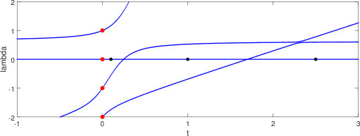
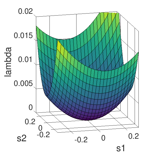
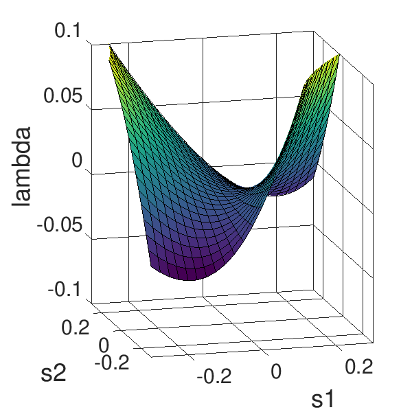
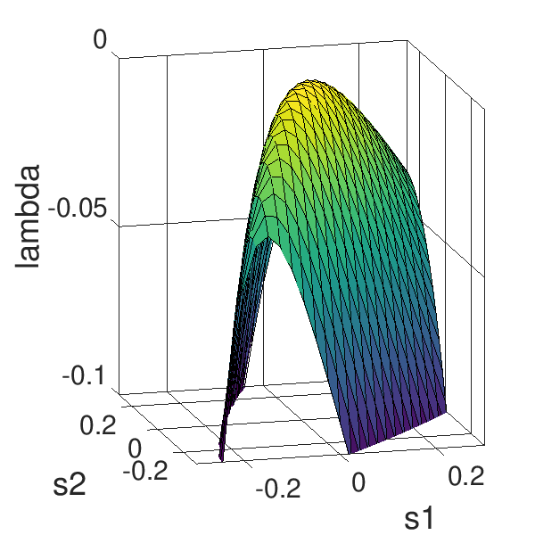
Figure 1. Top: the eigenvalues of $H(t,\vec{0})$ as functions of $t$; red (larger) dots highlight the eigenvalues of $H(0,\vec{0})$, black (smaller) dots indicate the values of $t$ where the lateral variation is explored in the bottom figures. Bottom: the continuation of the eigenvalue 0 in the spectrum of $H(0.1,\vec{s})$, $H(1,\vec{s})$ and $H(2.5,\vec{s})$, correspondingly, shown as functions of $\vec{s}=(s_{1},s_{2})$.

The one-parameter family $H(t,\vec{0})$ is a perturbation of $H(0,\vec{0})$ along the eigenvector $e_{1}$ of the eigenvalue $0$. As $t$ increases, the eigenvalue $0$ remains constant while the other eigenvalues increase, see Fig. 1(top). This type of figure is usually called spectral flow.

The spectral shift at $\lambda=0$ between $H(0,\vec{0})$ and $H(t,\vec{0})$ is visualized as the number of eigenvalues crossing $\lambda=0$ between $0$ and $t$. Thus, at the values of $t=0.1$, $1.0$ and $2.5$, highlighted by black dots in Fig. 1(top), the spectral shift is 0, 1 and 2 correspondingly. The spectrum of the lateral variations at these points (more precisely, the continuations of the eigenvalue 0 in the spectrum of $H(0.1,\vec{s})$, $H(1,\vec{s})$ and $H(2.5,\vec{s})$) is shown in the bottom row of Fig. 1. As predicted by Theorem 3.10, the point $\vec{s}=(0,0)$ is a minimum, saddle point and maximum correspondingly.

4.2. An application: magnetic–nodal theorem

We will show that a recent theorem of Berkolaiko and Colin de Verdière, which already has two different but complicated proofs [Ber13, CdV13], is a simple consequence of the results of this paper. We start with a simple example.

Example 4.1.

Consider the matrix

$$H(\alpha)=\begin{pmatrix}q_{1}&-1&0&0\\ -1&q_{2}&-1&-1\\ 0&-1&q_{3}&-e^{i\alpha}\\ 0&-1&-e^{-i\alpha}&q_{4}\end{pmatrix},$$

which is a matrix representation of the magnetic Schrödinger operator on the graph in Fig. 2, top left (precise definition will be given below). We are interested in the number of sign flips of the $n$-th eigenvector $f$ of $H(0)$, which in this case can be described as the number of pairs $(j,k)\in\{(1,2),(2,3),(2,4),(3,4)\}$ such that $f_{j}f_{k}<0$. We denote this number by $\phi_{n}$.

It was discovered in [Ber13] that $\phi_{n}$ is closely related to local behavior of eigenvalues of $H(\alpha)$, shown in Fig. 2, right. Whether the eigenvalue $\lambda_{n}(H(\alpha))$ experiences a minimum or a maximum at $\alpha=0$ is determined by whether the quantity $\sigma_{n}:=\phi_{n}-n+1$ is $0$ or $1$ (a part of the result is that $\sigma_{n}$ can only be $0$ or $1$ in this case). In other words, $\phi_{n}-n+1$ is the Morse index of $\lambda_{n}(H(\alpha))$.

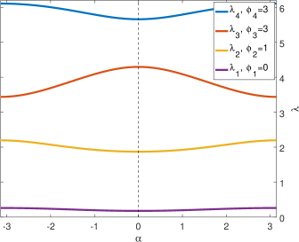
Figure 2. Top left: the graph corresponding to operator $H$ in Example 4.1. Bottom left: the graph corresponding to operator $S$. Right: eigenvalues of the matrix $H(\alpha)$ as function of $\alpha\in[-\pi,\pi]$; the legend lists the “sign flip counts” for the corresponding eigenfunction of $H(0)$. We used $q_{1}=1$, $q_{2}=2$, $q_{3}=4$ and $q_{4}=5$.

The relation to previous results comes from the fact that $H(\alpha)$ can be represented as

$$H(\alpha)=\begin{pmatrix}q_{1}&-1&0&0\\ -1&q_{2}&-1&-1\\ 0&-1&q_{3}-\gamma&0\\ 0&-1&0&q_{4}-1/\gamma\end{pmatrix}+\begin{pmatrix}0&0&0&0\\ 0&0&0&0\\ 0&0&\gamma&-e^{i\alpha}\\ 0&0&-e^{-i\alpha}&1/\gamma\end{pmatrix}=:S+P(\alpha),$$

where $\gamma$ is adjusted so that $P(0)f=0$ for a given eigenfunction $f$. The matrix $S$ is a Schrödinger operator on the tree shown in Fig. 2, bottom left. It was established by Fiedler [Fie75] that any tree satisfies Sturm nodal theorem: the $n$-th eigenfunction has $n-1$ sign flips. The spectral shift of $H$ with respect to $S$ can then be interpreted as “extra number of sign flips”, compared to the baseline number $n-1$. On the other hand, the spectral shift is equal to the Morse index of $\lambda_{n}(\alpha)$ by Theorem 1.1 (or Theorem 3.5).

Let us now extend and formalize the above example. Let $H$ be a real symmetric $N\times N$ matrix representing the Schrödinger operator (with generalized edge weights) on a connected graph $\Gamma=({\mathcal{V}},{\mathcal{E}})$ in the following sense,

• ${\mathcal{V}}=\{1,\ldots,N\}$,

• $H_{u,v}=H_{v,u}$,

• for $u\neq v$,

  $$H_{u,v}\neq 0\quad\Leftrightarrow\quad(u,v)\in{\mathcal{E}}.$$

Let $T$ be a spanning tree of $\Gamma$ and let $C={\mathcal{E}}(\Gamma)\setminus{\mathcal{E}}(T)$. There are exactly $\beta=|{\mathcal{E}}|-|{\mathcal{V}}|+1$ edges in the set $C$. We assume the graph $\Gamma$ is not a tree itself, i.e. $\beta>0$.

Orient each edge in $C$ in an arbitrary fashion and order the set $C$. Let $\vec{\alpha}$ be a point in the $\beta$-dimensional torus $\mathbb{T}^{\beta}:=(-\pi,\pi]^{\beta}$ and denote by $H(\vec{\alpha})$ the magnetic Schrödinger operator obtained from $H$ by letting

$$H(\vec{\alpha})_{u_{j},v_{j}}=e^{i\alpha_{j}}H_{u_{j},v_{j}},\qquad H(\vec{\alpha})_{v_{j},u_{j}}=e^{-i\alpha_{j}}H_{v_{j},u_{j}},$$ (49)

if $(u_{j},v_{j})\in C$ and $H(\vec{\alpha})_{u,v}=H_{u.v}$ otherwise. We note that $H(0)=H$.

Theorem 4.2 (And extended version of [Ber13, CdV13]).

Let $\vec{\alpha}^{\circ}\in\{0,\pi\}^{\beta}$, let $\lambda^{\circ}$ be the $n$-th eigenvalue in the spectrum of $H\left(\vec{\alpha}^{\circ}\right)$. Assume $\lambda^{\circ}$ is simple and the corresponding eigenvector $f$ has no zero entries. Consider $\Lambda(\vec{\alpha})$, the smooth continuation of the eigenvalue $\lambda^{\circ}$ in the spectrum of $H(\vec{\alpha})$. Then

1. $\Lambda(\vec{\alpha})$ has a critical point $\vec{\alpha}=\vec{\alpha}^{\circ}$,

2. the Morse index of the critical point is equal to the nodal surplus of $f$ defined as

   $$\sigma=\phi(f,\Gamma)-(n-1),$$ (50)

   where $\phi(f,\Gamma)$ is the flip count of $f$ with respect to the graph $\Gamma$,

   $$\phi(f,\Gamma)=\#\left\{(u,v)\in{\mathcal{E}}\colon-f_{u}f_{v}H(\vec{\alpha}^{\circ})_{u,v}<0\right\}.$$ (51)

Proof.

For an $e=(v_{1},v_{2})\in C$, define

$$s_{e}=\operatorname{sgn}\left(-H(\vec{\alpha}^{\circ})_{v_{1},v_{2}}f_{v_{1}}f_{v_{2}}\right),\qquad p_{e}=\sqrt{\left|H(\vec{\alpha}^{\circ})_{v_{1},v_{2}}{f_{v_{2}}}/{f_{v_{1}}}\right|},$$

and introduce a $\beta\times|{\mathcal{V}}|$ matrix $K(\vec{\alpha})$

$$K(\vec{\alpha})_{e,v}=\begin{cases}p_{e}s_{e}&\mbox{if }v=v_{1},\\ e^{i(\alpha_{e}-\alpha_{e}^{\circ})}H(\vec{\alpha}^{\circ})_{v_{1},v_{2}}/p_{e}&\mbox{if }v=v_{2},\\ 0&\mbox{otherwise},\end{cases}\qquad\mbox{where }e=(v_{1},v_{2})\in C.$$

A direct calculation shows that $K(\vec{\alpha}^{\circ})f=\vec{0}$.

Let $\Omega$ be the diagonal $\beta\times\beta$ matrix of signs $s_{e}$ and consider the matrix

$$S:=H(\vec{\alpha})-K(\vec{\alpha})^{*}\Omega K(\vec{\alpha}),\qquad\vec{\alpha}\in\mathbb{R}^{\beta}.$$ (52)

The elements of $S$ corresponding to the edges $e\in C$ are zero; moreover the matrix $S$ is independent of $\vec{\alpha}$. In other words, the matrix-function

$$H^{\mathbb{C}}(\vec{\alpha}):=S+K(\vec{\alpha})^{*}\Omega K(\vec{\alpha}),\qquad\vec{\alpha}\in\mathbb{C}^{\beta}$$ (53)

coincides with $H(\vec{\alpha})$ for real $\vec{\alpha}$.

Consider the function $\Lambda^{\mathbb{C}}(\vec{\alpha})=\lambda_{n}\big{(}H^{\mathbb{C}}(\vec{\alpha})\big{)}$. By Theorems 3.5 and 3.10 its Hessian at $\vec{\alpha}=\vec{\alpha}^{\circ}$ is the operator (33) which is a matrix with real entries. Being real, it coincides with the Hessian of the function $\Lambda(\vec{\alpha})=\lambda_{n}\big{(}H(\vec{\alpha})\big{)}$ of the real argument. Furthermore, its Morse index $\mu$ is equal to $m-n+\omega_{-}$, where $m$ is such that $\lambda^{\circ}=\lambda_{m}(S)$ and $\omega_{-}$ is the number of $e\in C$ with $s_{e}<0$.

The graph corresponding to the matrix $S$ is the spanning tree $T=\Gamma\setminus C$ we chose, and we have

$$\phi(f,\Gamma)=\phi(f,T)+\omega_{-}.$$

Because the matrix $T$ is acyclic and the eigenfunction $f$ has no zero entries, the eigenvalue $\lambda^{\circ}$ is simple in the spectrum of $S$, see [Fie75], and the critical point $\vec{\alpha}^{\circ}$ of the function $\Lambda(\vec{\alpha})$ is non-degenerate.

The same paper [Fie75] also established that $\phi(f,T)=m-1$, where $m$ is as above, i.e. the number of the $\lambda^{\circ}$ in the spectrum of $S$. Combining all of the above, we get

$$\mu=m-n+\omega_{-}=1+\phi(f,T)-n+\omega_{-}=\phi(f,\Gamma)-(n-1).$$

∎

References

- [BCCM20] G. Berkolaiko, Y. Canzani, G. Cox, and J. L. Marzuola, A local test for global extrema in the dispersion relation of a periodic graph, Preprint arXiv:2004.12931, 2020.
- [Ber13] G. Berkolaiko, Nodal count of graph eigenfunctions via magnetic perturbation, Anal. PDE 6 (2013), 1213–1233, preprint arXiv:1110.5373.
- [BGN18] J. Behrndt, F. Gesztesy, and S. Nakamura, Spectral shift functions and Dirichlet-to-Neumann maps, Math. Ann. 371 (2018), 1255–1300.
- [BIG03] A. Ben-Israel and T. N. E. Greville, Generalized inverses, second ed., CMS Books in Mathematics/Ouvrages de Mathématiques de la SMC, vol. 15, Springer-Verlag, New York, 2003.
- [BKS12] G. Berkolaiko, P. Kuchment, and U. Smilansky, Critical partitions and nodal deficiency of billiard eigenfunctions, Geom. Funct. Anal. 22 (2012), 1517–1540, preprint arXiv:1107.3489.
- [BS91] F. A. Berezin and M. A. Shubin, The Schrödinger equation, Mathematics and its Applications (Soviet Series), vol. 66, Kluwer Academic Publishers Group, Dordrecht, 1991, Translated from the 1983 Russian edition by Yu. Rajabov, D. A. Leĭtes and N. A. Sakharova and revised by Shubin. With contributions by G. L. Litvinov and Leĭtes.
- [BtEG20] J. Behrndt, A. F. M. ter Elst, and F. Gesztesy, The generalized Birman–Schwinger principle, preprint arXiv:2005.01195, 2020.
- [BW14] G. Berkolaiko and T. Weyand, Stability of eigenvalues of quantum graphs with respect to magnetic perturbation and the nodal count of the eigenfunctions, Philos. Trans. R. Soc. Lond. Ser. A Math. Phys. Eng. Sci. 372 (2014), 20120522, 17.
- [CdV13] Y. Colin de Verdière, Magnetic interpretation of the nodal defect on graphs, Anal. PDE 6 (2013), 1235–1242, preprint arXiv:1201.1110.
- [CHM74] D. Carlson, E. Haynsworth, and T. Markham, A generalization of the Schur complement by means of the Moore-Penrose inverse, SIAM J. Appl. Math. 26 (1974), 169–175.
- [Fie75] M. Fiedler, Eigenvectors of acyclic matrices, Czechoslovak Math. J. 25(100) (1975), 607–618.
- [GKMT01] F. Gesztesy, N. J. Kalton, K. A. Makarov, and E. Tsekanovskii, Some applications of operator-valued Herglotz functions, Operator theory, system theory and related topics (Beer-Sheva/Rehovot, 1997), Oper. Theory Adv. Appl., vol. 123, Birkhäuser, Basel, 2001, pp. 271–321.
- [GMN99] F. Gesztesy, K. A. Makarov, and S. N. Naboko, The spectral shift operator, Mathematical results in quantum mechanics (Prague, 1998), Oper. Theory Adv. Appl., vol. 108, Birkhäuser, Basel, 1999, pp. 59–90.
- [Hay68] E. V. Haynsworth, Determination of the inertia of a partitioned Hermitian matrix, Linear Algebra and Appl. 1 (1968), 73–81.
- [HF85] S.-P. Han and O. Fujiwara, An inertia theorem for symmetric matrices and its application to nonlinear programming, Linear Algebra Appl. 72 (1985), 47–58.
- [How70] J. S. Howland, On the Weinstein-Aronszajn formula, Arch. Rational Mech. Anal. 39 (1970), 323–339.
- [JMRT87] H. T. Jongen, T. Möbert, J. Rückmann, and K. Tammer, On inertia and Schur complement in optimization, Linear Algebra Appl. 95 (1987), 97–109.
- [KK66] R. Konno and S. T. Kuroda, On the finiteness of perturbed eigenvalues, J. Fac. Sci. Univ. Tokyo Sect. I 13 (1966), 55–63 (1966).
- [Mad88] J. H. Maddocks, Restricted quadratic forms, inertia theorems, and the Schur complement, Linear Algebra Appl. 108 (1988), 1–36.
- [Pus09] A. Pushnitski, Operator theoretic methods for the eigenvalue counting function in spectral gaps, Ann. Henri Poincaré 10 (2009), 793–822.
- [Sch17] J. Schur, Über Potenzreihen, die im Innern des Einheitskreises beschränkt sind, J. Reine Angew. Math. 147 (1917), 205–232.
- [Tia10] Y. Tian, Equalities and inequalities for inertias of Hermitian matrices with applications, Linear Algebra Appl. 433 (2010), 263–296.
- [Tre08] C. Tretter, Spectral theory of block operator matrices and applications, Imperial College Press, London, 2008.
- [Yaf92] D. R. Yafaev, Mathematical scattering theory, Translations of Mathematical Monographs, vol. 105, American Mathematical Society, Providence, RI, 1992, General theory, Translated from the Russian by J. R. Schulenberger.