Charged Higgs Observability via Charged Higgs Pair Production at Future Lepton Collider

Abstract

The observability of charged Higgs $H^{\pm}$ has been investigated at future lepton collider by assuming type-I 2HDM, at a centre of mass energy $\sqrt{s}=1.5$ TeV. The signal process chain is $e^{+}e^{-}\rightarrow Z^{*}/\gamma^{*}\rightarrow H^{+}H^{-}\rightarrow HW^{+}HW^{-}\rightarrow b\overline{b}jjb\overline{b}jj$. The process proceed through virtual gamma and Z-boson exchange in S-channel. Several benchmark points are selected and events are analyzed to reconstruct the mass of charged Higgs bosons $H^{\pm}$. The value of $\tan\beta$ is kept relatively high to enhance the branching ratio of $H\rightarrow b\overline{b}$ to benefit the signal processes. The main SM background processes produced is $t\overline{t}$. Signal selection and significance efficiencies are calculated at integrated luminosities of $100fb^{-1}$ and $500fb^{-1}$. The reconstructed and corrected mass of charged Higgs bosons $H^{\pm}$ is determined. Through analyzing the results, it is demonstrated that charged Higgs bosons can be discovered through pair production process via its bosonic decays. This study is supposed to provide the experimentalists a good way to examine the Higgs bosons beyond SM, as well as to check the validity of 2HDM models in considered parameter space.

I Introduction

Particle physics is concerned with the study of elementary particles and their interactions. Many theories were developed to explain the properties and interactions of all known particles. The Standard Model (SM) is founded to be consistent with experimental results till the time.constraints . In Standard Model, only one Higgs doublet exists and the masses of bosons and fermions are obtained by the Higgs mechanism search . SM have some unanswered questions like the neutrino oscillations, dark matter and the absence of gravity in the theory. These problems made the basis for the development of the theories beyond the Standard Model which may be capable to resolve these mysteries. The most simplest enhancement of Standard Model is the Two Higgs Doublet Model (2HDM). This model has two Higgs doublets and allow more physical Higgs states. Two Higgs Doublet Model (2HDM) is the simplest low energy effective model low and provides general description of Higgs sector and its interaction with fermions constraint . In 2HDM the complex scalar doublet $\phi_{1}$ of SM is augmented with another doublet , $\phi_{2}$. Due to second doublet all gauge bosons and fermions gain mass theory . There are eight degrees of freedom in 2HDM. The three degrees of freedom are eaten up by the electroweak bosons in electro-weak symmetry breaking. The remaining five degrees of freedom give rise to five physical Higss bosons  observe . The 2HDM contains $2$ even neutral scalar Higgs bosons $h$ , $H$ , an odd pseudoscalar neutral Higgs boson $A$ and a pair of charged Higgs bosons $H^{\pm}$  lc . The presence of charged higgs bosons is a special characteristics of 2HDM because these are not included in SM.
With the discovery of Higgs boson at Large Hadron Collider (LHC), in 2012, it was confirmed that the thought of Higgs mechanism is a right approach. This discovery begins a race among the scientists to verify that either there exist only a single observed Higgs or more Higgs states are also possible as predicted by various extended theories. Till date no such boson has been found. Compact Linear Collider (CLIC) is one of the proposed future lepton collider to accelerate the electron and positron beams. CLIC is aimed to be constructed and operated at three steps, i.e. at $380$ GeV, $1.5$ TeV and $3$ TeV collision energies respectively. Lepton collider can measure the Higgs couplings with more precision than already achieved by LHC. It is thought that due to its clean environment, CLIC is more capable for finding new physics that is why in this study, the phenomenology for this collider is made CLIC . The aim of designing CLIC is to achieve the electron-positron head-on collisions at several tera electron volts (TeV) energies.
The focus of the paper is on the study of charged Higgs pair bosons $H^{\pm}$ and their bosonic decays. The theoretical framework for this work is type 1 2HDM. The investigation of the observability of charged Higgs bosons $H^{\pm}$ takes place by the signal process $e^{+}e^{-}\rightarrow Z^{*}/\gamma^{*}\rightarrow H^{+}H^{-}\rightarrow HW^{+}HW^{-}\rightarrow b\overline{b}jjb\overline{b}jj$. Where $j$ represents light jet and b is the bottom quark. This is the most favorable production scenario with bosonic decays for charged Higgs study at linear colliders. The process will proceed by exchange of gamma and Z-boson in s-channel. The Figure 1 shows the Feynman diagram of this process.

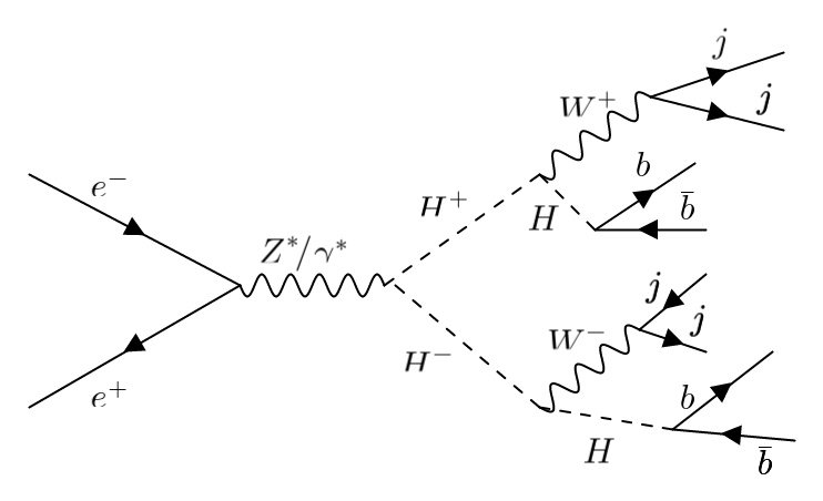
Figure 1: The s-channel Feynman diagram contributing to the signal process

In this analysis, each of the charged Higgs decays into $W^{\pm}H$ and the final state becomes $2W^{\pm}H$. Several benchmark points in the parameter space of 2HDM majid are considered for charged Higgs bosons observability at centre of mass energy $\sqrt{s}=1.5$ TeV. The signal and background events are generated independently for each scenario observe . The charged Higgs boson candidates are identified by comparing signal with background events in different distributions. To reconstruct the charged Higgs bosons, simulated events are analyzed. For this purpose, first b-jets are identified. These b-jets are reconstructed by choosing proper b tagging algorithms and b-jet clustering. The combinations of b-jets are identified so that the dijet invariant mass gives us the Higgs candidate. The mass range for studied charged Higgs is $125<m_{H^{\pm}}<400$ GeV at $\sqrt{s}=1.5$ TeV at the integrated luminosity of $500fb^{-1}$

II Two Higgs Doublet Model

There are four types of 2HDM. In type I, the gauge bosons and all fermions attain mass from one Higgs doublet while contribution of the other Higgs doublet is via mixing constraint . Discrete Symmetry $\phi_{1}\rightarrow-\phi_{1}$ is involved in type I. One higgs doublet (conventionally $\phi_{2}$ ) couples with all quarks (up-type quark and down-type quark) and charged leptons in type-I 2HDM and flavour is conserved naturally. There are two discrete situations to achieve naturally flavor conservation in 2HDM. First, when only one Higgs doublet (conventionally $\phi_{2}$ ) couple with all quarks (up-type and down-type) and charged leptons, it is named as the type-I 2HDM. In second case, termed as type-II 2HDM, all the up-type quarks couple to one Higgs doublet ($\phi_{2}$ ) and all down-type quarks along with charged leptons couple with the other Higgs doublet ($\phi_{1}$ ). It can be observed that a discrete symmetry $(\phi_{1}\rightarrow-\phi_{1})$ can be implemented on type-I as well as on type-II. It is conventionally assumed that the up-type quarks are always coupled with the second doublet $\phi_{2}$ in all types. Different types of 2HDM are shown in Table  1.

Types of Model	Description	$u_{R}^{i}$	$d_{R}^{i}$	$e_{R}^{i}$
Type I	Fermiophobic	$\Phi_{2}$	$\Phi_{2}$	$\Phi_{2}$
Type II	MSSM like	$\Phi_{2}$	$\Phi_{1}$	$\Phi_{1}$
Type III	Lepton-specific	$\Phi_{2}$	$\Phi_{2}$	$\Phi_{1}$
Type IV	Flipped	$\Phi_{2}$	$\Phi_{1}$	$\Phi_{2}$

Table 1: Different types of 2HDM on the basis of coupling of Fermions with charged leptons

The expression for the general scalar potential with two higgs doublets $\phi_{1}$ and $\phi_{2}$ can be written as

$$V_{2HDM}=m_{11}^{2}\phi_{1}^{\dagger}\phi_{1}+m_{22}^{2}\phi_{2}^{\dagger}\phi_{2}-[m_{12}^{2}\phi_{1}^{\dagger}\phi_{2}+h.c]+\frac{1}{2}\lambda_{1}(\phi_{1}^{\dagger}\phi_{1})^{2}+\frac{1}{2}\lambda_{2}(\phi_{2}^{\dagger}\phi_{2})^{2}$$ (1)

$$+\lambda_{3}(\phi_{1}^{\dagger}\phi_{1})(\phi_{2}^{\dagger}\phi_{2})+\lambda_{4}(\phi_{1}^{\dagger}\phi_{2})(\phi_{2}^{\dagger}\phi_{1})+[\frac{1}{2}\lambda_{5}(\phi_{1}^{\dagger}\phi_{2})^{2}+[\lambda_{6}(\phi_{1}^{\dagger}\phi_{1})+\lambda_{7}(\phi_{2}^{\dagger}\phi_{2})](\phi_{1}^{\dagger}\phi_{2})+h.c]$$

In Equation (1), $\lambda_{i}$, where ($i=1,2.....,7)$ are coupling parameters having no dimensions and $m_{11}^{2}$, $m_{22}^{2}$ and $m_{12}^{2}$ are squared mass parameters. Out of these parameters the $m_{12}^{2}$ and $\lambda_{i}$ (Where $i=5,6,7$) are preferably complex while the remaining parameters are real. The $m_{12}^{2}$ term is of great importance because its nonzero values causes the soft breakdown of the $Z_{2}$ symmetry $(\phi_{1}\rightarrow-\phi_{1})$ or $(\phi_{2}\rightarrow-\phi_{2})$. The potential becomes explicitly CP violating in the presence of non zero imaginary parts of the complex parameters therefore in order to treat the potential as CP conserving here it is supposed that all the parameters used are real. For complete specification of the model the different parameters $m_{12}^{2}$, $\tan\beta$, physical Higgs masses$m_{H^{\pm}}$,$m_{A}$,$m_{h}$,$m_{H}$, mixing angle $\alpha$,$\sin(\beta-\alpha)$, $\lambda_{6}$ and $\lambda_{7}$ must be calculated in the physical basis 2HDM ; model .If the value of $\sin(\beta-\alpha)$ is taken to be one then it is called the exact alignment limit in which the lighter CP-even Higgs $h$ behaves like SM Higgs boson and if the value of $\sin(\beta-\alpha)$ is taken to be zero then the heavier CP-even Higgs behaves like SM Higgs boson. This study is performed within alignment limit i.e. $\sin(\beta-\alpha)=1$. The mass of lighter Higgs is taken as the mass of SM higgs boson i.e. $m_{h}=125GeV$. In type-I 2HDM all the fermions couple with a single Higgs doublet $(\phi_{2})$ same as in SM however the other Higgs doublet does not couple at all. This is due to the implementation of distinct $Z_{2}$ symmetry. For Yukawa interactions in type-I 2HDM the lagrangian is given in Equation (2)

$$L_{Yukawa}=Y_{e}\overline{L_{L}}\phi_{2}e_{R}+Y_{u}\overline{Q_{L}}~{}\widehat{\phi}_{2}u_{R}+Y_{d}\overline{Q_{L}}\phi_{2}d_{R}+h.c]$$ (2)

where $e_{R},_{u}{R},d_{R}$ are the left handed leptons, up-type and down-type quarks singlet respectively with$Y_{e},Y_{u},Y_{d}$ as their corresponding Yukawa coupling matrices. The terms $\overline{L_{L}},\overline{Q_{L}}$ are left-handed lepton and quark doublets respectively and $\widehat{\phi}_{2}=\iota\sigma_{2}\phi_{2}^{\ast}$ (Where $\sigma_{2}$ is Pauli matrix). If the weak eigen states of $\phi_{2}$ are expressed in physical terms then above Equation  (2) becomes

$$L_{Yukawa}=-\{\underset{\varphi=u,d,l}{\sum}\dfrac{m_{\varphi}}{\upsilon}(\kappa_{\varphi}^{h}\overline{\varphi}\varphi h^{0}+\kappa_{\varphi}^{H}\overline{\varphi}\varphi H^{0}-\iota\kappa_{\varphi}^{A}\overline{\varphi}\gamma_{5}\varphi A\}-\{\dfrac{V_{ud}}{\sqrt{2}\upsilon}\overline{u}(m_{u}\kappa_{u}^{A}P_{L}+m_{d}\kappa_{d}^{A}P_{R})dH^{+}\\ -\dfrac{m_{l}}{\sqrt{2}\upsilon}\kappa_{l}^{A}\overline{\nu}_{L}l_{R}H^{+}+h.c\}$$ (3)

In above Equation the $\kappa$ factors represent the Yukawa couplings and their values for 2HDM type-I are given in Table  2 .

$\kappa_{u}^{h}$	$\kappa_{d}^{h}$	$\kappa_{l}^{h}$	$\kappa_{u}^{H}$	$\kappa_{d}^{H}$	$\kappa_{l}^{H}$	$\kappa_{u}^{A}$	$\kappa_{d}^{A}$	$\kappa_{l}^{A}$
$\dfrac{\cos\alpha}{\sin\beta}$	$\dfrac{\cos\alpha}{\sin\beta}$	$\dfrac{\cos\alpha}{\sin\beta}$	$\dfrac{\sin\alpha}{\sin\beta}$	$\dfrac{\sin\alpha}{\sin\beta}$	$\dfrac{\sin\alpha}{\sin\beta}$	$\cot\beta$	$-\cot\beta$	$-\cot\beta$

Table 2: Values of Yukawa couplings for 2HDM type I

For all types of 2HDM, W and Z boson couplings with neutral Higgs bosons are identical. Light Higgs ‘h’ and heavy Higgs ‘H’ couplings with either ZZ or WW are equal to $\sin(\beta-\alpha)$ and $\cos(\beta-\alpha)$ times the corresponding standard model couplings respectively. The coupling for the interaction between higgs boson pair and gauge boson like $H^{\pm}W^{\pm}H$ can be estimated by using the gauge coupling structure and the angles $\alpha$ and $\beta$. The coupling relations bb are given below in Equations  (4),(5) and (6).

$$g(H^{\pm}HW^{\pm}):\dfrac{g}{2}(p_{H}-p_{H^{\pm}})^{\mu}\sin(\beta-\alpha)$$ (4)

$$g(H^{\pm}hW^{\pm}):\dfrac{g}{2}(p_{h}-p_{H^{\pm}})^{\mu}\cos(\beta-\alpha)$$ (5)

$$(gH^{\pm}HW^{\pm}):\dfrac{g}{2}(p_{A}-p_{H^{\pm}})^{\mu}$$ (6)

Where $p_{H}$, $p_{h}$ and $p_{A}$ represent the momentum of incoming particles respectively.

III Strategy and Signal Extraction

In this study events are produced with the help of Pythia-8210  pyt and relative efficiencies are also calculated in it. 2HDMC-1.7.0  con is used to calculate the branching ratios as well as decay widths of Higgs sector in type-I of Two Higgs doublet Model at desired benchmark points and its output in SLHA format is fed to Pythia. For the analysis and reconstruction of jets produced in the events Pythia is linked with fastjet-3.3.3. In order to record the events data, the interface of HepMC-2.06.06  Hep is given to Pythia. The output of Pythia is than analyzed and histograms are plotted by using Root- 6.20/04  rt .

III.1 Signal Process

The observability of the charged Higgs bosons is investigated through signal process $e^{+}e^{-}\rightarrow H^{+}H^{-}$. The process chain is $e^{+}e^{-}\rightarrow Z^{*}/\gamma^{*}\rightarrow H^{+}H^{-}\rightarrow HW^{+}HW^{-}\rightarrow b\overline{b}jjb\overline{b}jj$. There are many other possibilities for this process. In the process $e^{+}e^{-}\rightarrow Zh$, h has taken as SM higgs so it can not be taken for study when Higgs boson beyond SM is studied. In processes $e^{+}e^{-}\rightarrow ZH$ or $e^{+}e^{-}\rightarrow Ah$, the H Z Z and $hZA$ vertices are involved and both are proportional to $\cos\left(\beta-\alpha\right)$. At $\sin\left(\beta-\alpha\right)=1$, both processes vanish when requirement is like SM observe . The choice of process $e^{+}e^{-}\rightarrow Z^{*}/\gamma^{*}\rightarrow H^{+}H^{-}$ is most suitable and favorable for study of charged Higgs at linear collider. The process takes place through exchange of Z and gamma bosons in s-channel. Each heavy neutral Higgs boson $H$ is allowed to disintegrate only into two b-jets and W boson is allowed to decay into two light jets. The final state contains four b-jets, and fout light jets.
In this study the masses of charged Higgs $H^{\pm}$ and pseudo scalar Higgs A are considered same in order to avoid the decay of charged Higgs bosons into pseudo scalar Higgs A. The selected benchmark points which fulfill the theoretical and experimental constriants are considered. The 2HDMC-1.7.0 hd is linked with packages HiggsBound-4.2.0 and HiggsSignal-1.4.0. It is used to make sure that all the benchmark points are consistent with all experimental and theoretical constraints. The range of parameter $m_{12}^{2}$ for each benchmark points satisfies the theoretical constraints. The mass splitting between heavy neutral Higgs and charged Higgs is taken in such a way that the bosonic decay of both charged Higgs $H^{\pm}\rightarrow W^{\pm}H$ is kinematically permitted. The ranges of heavy neutral and charged Higgs bosons, $\tan\beta$, $m_{12}^{2}$ and $\sin(\beta-\alpha)$ for different benchmark points are listed in Table 3.

	BP1	BP2	BP3	BP4
$m_{h}$(GeV)	$125$	$125$	$125$	$125$
$m_{H}$(GeV)	$150$	$200$	$250$	$300$
$m_{A}$ (GeV)	$250$	$325$	$400$	$400$
$m_{H^{\pm}}$ (GeV)	$250$	$325$	$400$	$400$
$\tan\beta$	$40$	$40$	$40$	$40$
$m_{12}^{2}$	$560$	$996-999$	$1560$	$2245-2248$
$\sin(\beta-\alpha)$	$1$	$1$	$1$	$1$

Table 3: The Higgs bosons masses, range of $m_{12}^{2}$ and branching fractions for different benchmark points within the allowed region.

The branching ratios for decays $(H^{\pm}\rightarrow W^{\pm}H)$ and $(H\rightarrow b\overline{b})$ as well as decay widths of higgs sector are obtained by using 2HDMC-1.7.0 hd for selected benchmark points and are given in Table 4.

BPpoints	$BR(H^{\pm}\rightarrow W^{\pm}H)$	$BR(H\rightarrow b\overline{b})$
BP1	9$.89\times 10^{-1}$	$7.112\times 10^{-1}$
BP2	$9.95\times 10^{-1}$	$6.16\times 10^{-1}$
BP3	$9.97\times 10^{-1}$	$5.08\times 10^{-1}$
BP4	$9.75\times 10^{-1}$	$3.79\times 10^{-1}$

Table 4: The branching ratios at each benchmark points.

All this information about a benchmark point is also included in its Susy LesHouches (SLHA) file and is provided to Pythia8210  pyt as input for generating events. The cross section for the process at given benchmark points is calculated by using Comphep-4.5.2  cp ; cf shown in Table 5.

BP points	$\sigma$	$\sigma$	$\sigma$	$\sigma_{max}$	$\sqrt{s}$
	at$1$TeV	at$1.5$TeV	at$3$TeV
	(fb)	(fb)	(fb)	(fb)	GeV
BP1	17.294	$10.978$	$3.1368$	$21.966$	$800$
BP2	11.699	$9.5886$	$3.0445$	$12.977$	$1040$
BP3	5.761	$7.9288$	$2.9294$	$8.5611$	$1250$
BP4	5.761	$7.9288$	$2.9294$	$8.5611$	$1250$

Table 5: The cross section, maximum cross section and corresponding C.M. energy of $e^{+}e^{-}\rightarrow H^{+}H^{-}$ at different benchmark points.

Energy is plotted versus cross section as shown in Figure  2.

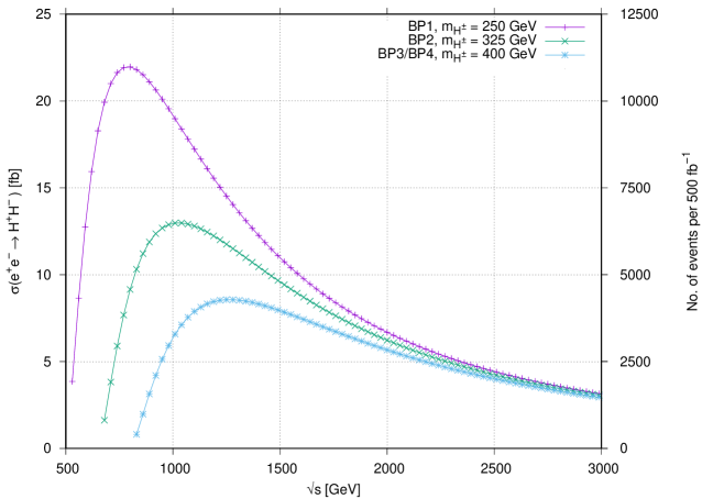
Figure 2: The cross section versus energy at different benchmark points within the allowed region.

It shows that with increase in energy, the cross section increases rapidly. It has maximum value when energy becomes equal to the threshhold energy. Threshold energy is the energy, required to produce the process. The cross section decreases with further increase in energy and it almost becomes linear at 3 TeV. It is due to the reason that the cross section of a process is inversely proportional to the square of the center of mass energy. At 3 TeV center of mass energy, the crosssections for all benchmark points have the same value, it means that the cross sections become independent of the center of mass energy and plots at this energy becomes linear.”

The main SM background process in the signal channel is the production of pair of top quark $t\overline{t}$ through electron-positron annihilation $e^{+}e^{-}\rightarrow t\overline{t}$. Events for all this background processe are also generated in Pythia because all the known information about SM particles, their couplings and SM processes are already stored in Pythia built in flags.

III.2 Event Selection process for identification of jets

The generated events are stored in HepMC-2.06.06  Hep . The jets produced in the events are reconstructed by using the FASTJET  mm . In this study anti-$k_{i}$, jet algorithm  anti is used to reconstruct the jets. Different kinematic selection cuts are applied which arises certain fluctuations in the signal. The selection cuts are applied in such a way that enhances the signal to background ratio while signal events are maintained at an appropriate level. Selection efficiencies are calculated and importance of signal is determined by computing signal significance. These cuts define the band of ranges which are invariant quantities, measured in events. It must fulfil the number of several final state particles. These particles are identified in phase of primary reconstruction using “object identification cuts”. Then the kinematic selection cuts are applied to refine the rejection and selection of background events to finalise the results.

The first step in event selection is the kinematic cut on jets which omit the soft $p_{T}$ jets and the ones that are in forward region along the collision beams. For this we apply following cuts on transverse momentum and pseudorapidity of jets.

$$p_{T}^{jet}>20GeV,|\eta_{jets}|<2.5$$ (7)

Once we have jets within the desired kinematic range, we split the reconstructed jets by identifying them as light and b-tagged jets. In order to achieve this, we do a $\Delta R$ matching of the jets with the generated particles which is defined as

$$\Delta R=\sqrt{(\Delta\eta)^{2}+(\Delta\phi)^{2}}$$ (8)

We identify the jets which are within $\Delta R<0.4$ of the b-quarks in the event as b-jets and the ones that are farther away from b-quarks as light jets. Once we have identified the jets, we apply the multiplicity cut on the jet. For $j\bar{j}j\bar{j}b\bar{b}b\bar{b}$ channel we require the event to have at least four light jets and at least four b-jets. In the analysis, we use the selected light-jets (b-jets) to find a combination that minimise the $\chi^{2}$ defined as follows.

$$\chi^{2}=\left(\frac{m_{jj,1}-m_{W}}{\sigma_{m_{W}}}\right)^{2}+\left(\frac{m_{jj,2}-m_{W}}{\sigma_{m_{W}}}\right)^{2}\left(\frac{m_{bb,1}-m_{H}}{\sigma_{m_{H}}}\right)^{2}+\left(\frac{m_{bb,2}-m_{H}}{\sigma_{m_{H}}}\right)^{2}$$ (9)

where $m_{jj,bb}$ are the dijet mass, $m_{W}$ is the mass of $W$ boson, and $m_{H}$ is the mass of the heavy Higgs boson according to the BP taken, and the $\sigma_{m_{W,H}}$ are the widths of the respective mass distributions. The cut of $\chi^{2}<10$ is applied to select only events with good reconstructed $W$ and $H$ bosons. The charged Higgs boson $H^{\pm}$ is then reconstructed using the combination of $W$ and $H$ which gives mass nearest to $H^{\pm}$ nominal mass according to the BP. After applying different selections cuts, The efficiencies are calculated. For getting more better simulation results, more than hundred thousand events are generated and analyzed for each selected scenario. Applying all cuts on generated events, relative efficiencies for corresponding selection cut are calculated. At the end, total signal selection efficiency is also calculated for each benchmark point. The results are shown in Table 6.

Cuts	BP1	BP2	BP3	BP4
Four lightjets	0.1467	0.2557	0.3278	0.3052
Four b-jets	0.5666	0.6478	0.6655	0.6544
$\chi^{2}$	0.2224	0.1737	0.1085	0.6162
CH $\chi^{2}$	0.5027	0.4526	0.3599	0.6767
Total efficiency	0.00929	0.01302	0.00852	0.00833
$\sigma\times B.R.$	4.58	2.17	0.66	0.37

Table 6: The efficiencies for different selection cuts at different mass hypothesis

The signal process has reasonable selection efficiency at all the selected benchmark points. From Table 6 it can be seen that from randomly generated signal events, all the events have four b jets and light jets. This is due to the fact that heavy scalar Higgs bosons, in signal processes decay into b-jets and W bosons decay into light jets.

IV Results and discussion

In the finalized results, topology of our assumed first signal process contains four b-jets and four light jets. Jet multiplicity distributions of signals processes and different SM backgrounds are shown in Figure  3.

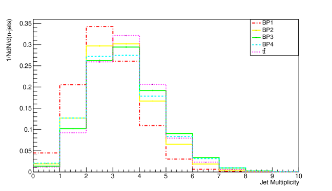
Figure 3: The jet multiplicity for events(signal and background)

The distribution of b-jets slightly depends on neutral Higgs boson mass in the assumed signal event. The production of b-jet is suppressed kinematically in the production of Higgs boson, the availability of phase space is smaller due to which it decays to bottom quarks.

Transverse energy $E_{T}$ of jets for second process is shown in Figure  5

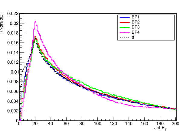
Figure 4: The Pseudorapidity $\eta$ of signal along with all background events

The jet Pseudorapidity $\eta$ for different signal and background processes is shown in Figure 5.

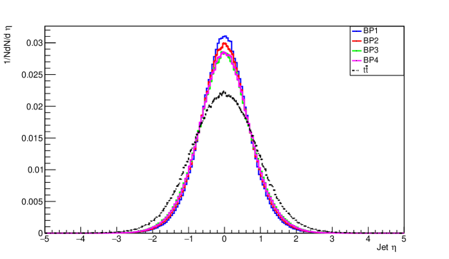
Figure 5: The Pseudorapidity $\eta$ of signal along with all background events

After extracting out the data of $\Delta R$, the profiling process of $\Delta R$ is discussed. By the analysis of plot of $\Delta R$ shown in Figure 6, the b-jets can easily be identified by finding the minima of the plot. To identify the b-jets from all sorted jets, those jets are choosen which satisfy $\Delta R<0.4$.

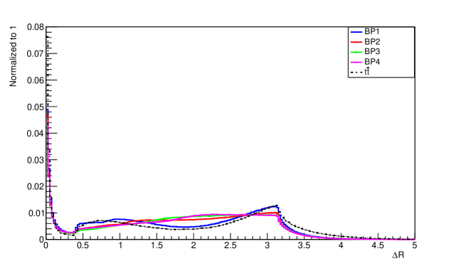
Figure 6: The distribution of $\Delta$ R( jets, quarks) variables used to tag bjet for all signal and background processes.

A jet is identified as a b-jet having possibility of $70\%$ if it has resemblance with a b quark and with chance of $10\%$ if it resemblance with a c quark. The above mentioned values are supposed as the b tagging efficiency and fake rate successively. As signal comprises on four b-jets from the hadronic decay of each heavy Higgs boson denoted by $H_{1}$ and $H_{2}$. In the Figure 7 the number of b-jets in signals and background events are shown.

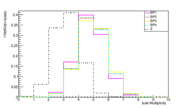
Figure 7: The bjets multiplicity at different benchmark points in various signals and background events

After the selection cuts, the only background which can contribute up to a reasonable level is $t\overline{t}$ having a very small number of events with four b-jets. For signal processes, it can be seen that each one has almost $60\%$to $70\%$ four b-jets efficiency. Other SM background may exist but they have very small number of events as compared to the signals. In the signal process, these jets come from hadronic decay of both W bosons.

IV.1 Reconstruction of W Bosons

For all scenarios the reconstructed masses peaks are exactly at 80 GeV which is close to the known mass of the W boson in SM (80.4 GeV). For backgrounds. the number of events with reconstructed W masses are very small as compared to our signals and on normalizing the above graphs, the reconstructed W masses for background processes cannot be seen. The histograms are filled for reconstructed masses of both $W^{\pm}$ for all benchmark points and shown in Figure 8 and  9. The representation for $W^{\pm}$ in histograms is taken as $W_{1}$ and $W_{2}$.

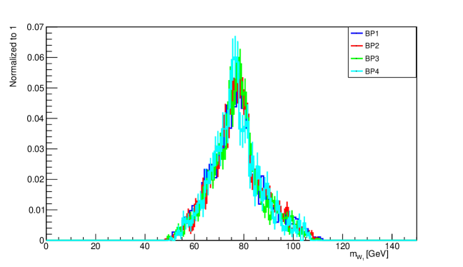
Figure 8: The plots of reconstructed invariant mass of$W_{1}$

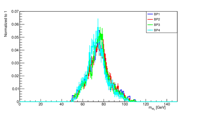
Figure 9: The plots of reconstructed invariant mass of $W_{2}$ in all signal events.

IV.2 Reconstruction of Heavy Neutral scalar Higgs Bosons

The invariant mass of neutral scalar Higgs bosons is reconstructed. In this work, the generation of signal and background processes is involved which display natural interference and selection techniques where different mass speculations are displayed for Higgs invariant mass remaking.
The process of mass reconstruction of Higgs bosons is considered as important to attain the reliable separation between the main assumed signal and the background processes. Peak of the signal resonance would be produced by the proper mass variable. By this process, large signal will be produced over the background ratio. The pair of b-jets comes out from the heavy Higgs Boson in the signal events. Due to that fact, the invariant mass of this pair should be lesser and lie within mass casement adjusted by neutral Higgs mass. Mass of the Higgs Boson can be calculated by the conventional formula given as

$$m_{H}=\sqrt{E^{2}-p_{x}^{2}-p_{y}^{2}-p_{z}^{2}}$$ (10)

The reconstructed invariant mass of the Higgs boson is represented by ”$m_{rec}$”, and the actual value of the Higgs boson mass is represented by ”$m_{Gen}$”. Then, for each possible combination, the sum of squared differences between observed and predicted Higgs-boson masses is calculated. Then, light jet and bjet pairings that meet the following conditions are chosen.

$\chi^{2}_{min}>10$

Only those events are selected which have four b-jets. In $\eta-\phi$ space, $\Delta R$ is calculated for all probable combinations of b-jet pairs for each event. The selection cut is introduced to justify that the combination of b-jet pairs are truly coming from Higgs boson decay so their reconstructed masses should be nearly equal to input mass of heavy Higgs boson ($m_{H}$). The small fraction of reconstructed masses not lying in this window is eliminated from efficiency calculation for each signal.the representation of neutral Higgs bosons are taken as $m_{H_{1}}$ and $m_{H_{2}}$.

The reconstructed mass distributions of $H_{1}$ and $H_{2}$ are shown in Figures 10 and 11 accordingly.

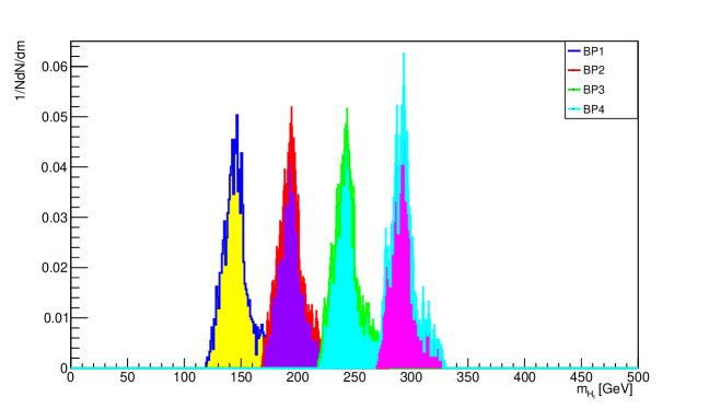
Figure 10: The reconstructed invariant mass of first heavy Higgs boson mass $m_{H_{1}}$ for all signal events and background.

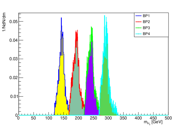
Figure 11: The reconstructed invariant mass of first heavy Higgs boson mass $m_{H_{2}}$ for all signal events and background.

The generated masses, reconstructed masses and corrected masses of Heavy neutral Higgs bosons for each selected scenario are computed in Table 7 and Table 8.

Signal Scenario	Gen. Mass(GeV)	Recons. Mass (GeV)	Corr.recons. Mass(GeV)
BP1	$150$	$143.9\pm 0.2459$	$151.45\pm 0.49$
BP2	$200$	$193.42\pm 0.2232$	$200.97\pm 0.47$
BP3	$250$	$241.63\pm 0.2476$	$249.18\pm 0.49$
BP4	$300$	$290.85\pm 0.2920$	$298.4\pm 0.5$

Table 7: Generated mass, reconstructed mass and corrected reconstructed mass of heavy neutral Higgs boson $H_{1}$ for all benchmark points.

Signal Scenario	Gen. Mass (GeV)	Recons. Mass (GeV)	Corr.recons. Mass(GeV)
BP1	$150$	$143.24\pm 0.24$	$151.83\pm 0.48$
BP2	$200$	$191.6\pm 0.2245$	$200.19\pm 0.47$
BP3	$250$	$240.8\pm 0.2296$	$249.39\pm 0.48$
BP4	$300$	$290\pm 0.2998$	$298.59\pm 0.5$

Table 8: The generated mass, reconstructed mass and corrected reconstructed mass of heavy neutral Higgs boson$H_{2}$ for all benchmark points.

The reconstructed masses are obtained by fitting suitable gaussian function on the distribution curves of $m_{H_{1}}$ and $m_{H_{2}}$ and taking their mean values. From Table 7 and Table 8 it can be observed that the reconstructed masses are less than the generated masses to some extent. These errors are caused by the uncertainties in different stages of analysis process like jet reconstruction algorithm, b-jet tagging procedure, fit functions, momentum and energy calculations of particles etc. These uncertainties can be reduced by making further developments in jet cluster sequence, b-jet tagging algorithm, measuring and fitting methods etc. However, this study is not concerned with the implementation of such modifications. An average difference of all measured masses of $m_{H_{1}}$ and $m_{H_{2}}$ is determined from their generated values and it is found that these are 7.55 GeV and 8.59 GeV less from their generated values respectively and average mass error is 0.2521 and 0.2483 respectively. This average difference is added in the reconstructed masses of $m_{H_{1}}$ and $m_{H_{2}}$ to find the corrected reconstructed mass values. It can be observed that the corrected reconstructed masses of both heavy scalar Higgs bosons are well agreed with their generated masses.

IV.3 Reconstruction of Charged Higgs Bosons

The reconstruction of charged Higgs masses is possible from W and H bosons. Now those events are selected that have four b-jets as well as four light jets simultaneously. Mass of positively charged Higgs boson, expressed as $m_{H^{+}}$ is determined from its supposed decay products i.e. $W^{+}$ boson and one heavy Higgs boson $m_{H_{1}}$. Mass of negatively charged Higgs boson expressed as $m_{H^{-}}$ is determined from its supposed decay products i.e. $W^{-}$ boson and other heavy Higgs boson $m_{H_{2}}$. As the mass distributions of both heavy Higgs bosons are almost similar to each other so the choice of heavy Higgs boson to reconstruct the charged Higgs boson will not affect the charged Higgs rebuilt masses significantly.

The Figure 12 shows the reproduced distributions for mass of charged Higgs $m_{H^{+}}$ and Figure 13 for mass of charged Higgs $m_{H^{-}}$. The charged Higgs $m_{H^{+}}$ is represented as CH1 and charged Higgs $m_{H^{-}}$ is represented as CH2.

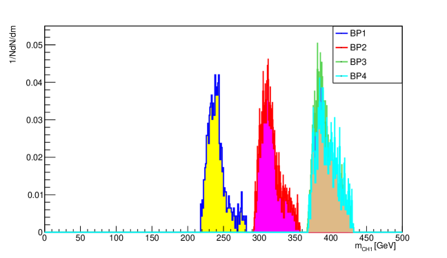
Figure 12: The reconstructed mass of charged Higgs boson $H^{+}$for all benchmark points.

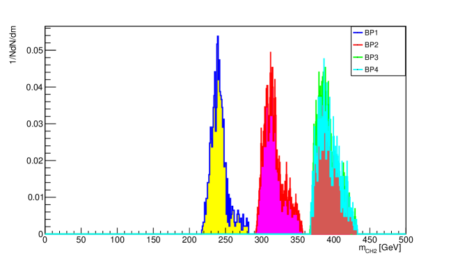
Figure 13: The reconstructed mass of charged Higgs boson $H^{-}$for all benchmark points.

The masses of charged Higgs $m_{H^{+}}$ and $m_{H^{-}}$ are less from their generated mass by an average of 10.65 GeV and 11.31 GeV respectively and average mass error is 0.51 and 0.45 respectively.. These values are added in the reconstructed masses of $m_{H^{+}}$ and $m_{H^{-}}$ respectively to get corrected reconstructed masses. Table  9 and Table 10 contain the data of generated, reconstructed and corrected reconstructed masses of charged Higgs bosons.

Signal Scenario	Gen. Mass(GeV)	Recons. Mass (GeV)	Corr.recons. Mass(GeV)
BP1	$250$	$237.5\pm 0.4$	$248.15\pm 0.9$
BP2	$325$	$313\pm 0.4$	$323.65\pm 0.9$
BP3	$400$	$388pm0.6$	$398.65\pm 1$
BP4	$400$	$393.9\pm 0.65$	$404.55\pm 1$

Table 9: The generated mass, reconstructed mass and corrected reconstructed mass of charged Higgs boson $H^{+}$ for all benchmark points.

Signal Scenario	Gen. Mass(GeV)	Recons. Mass(GeV)	Corr.recons. Mass(GeV)
BP1	$250$	$238.5\pm 0.29$	$249.81\pm 0.7$
BP2	$325$	$313.5\pm 0.4$	$324.81\pm 0.8$
BP3	$400$	$386.8\pm 0.42$	$398.11\pm 0.8$
BP4	$400$	$390.95\pm 0.7$	$402.26\pm 1$

Table 10: The generated mass, reconstructed mass and corrected reconstructed mass of charged Higgs boson $H^{-}$ for all benchmark points.

Gen. Mass is the mass of neutral heavy higgs mass taken as BP which satisfy the constraints. Here it was generated .

IV.4 Signal Significance

To examine the visibility of charged higgs boson at a linear collider, significance of the signal is studied for charged Higgs mass distributions. Signal to background ratio, total efficiency and signal significance is calculated for integrated luminosity 100 500 fb^-1 1000 and 5000 and results is presented in Table   11 . Although in this study the detector effects are not included however this process can be used as a discovery channel for charged Higgs boson at CLIC. The Figure 14 shows the bin wise filling of charged scalar Higgs mass values of all signal events and total background events at $100fb^{-1}$, $500fb^{-1}$.

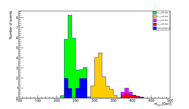
Figure 14: Mass of charged Higgs boson for all signals and for total background events filled bin wise at $500fb^{-1}$.

It can be seen that the signals are dominated over background events throughout the charged Higgs mass range. Table 11 shows the signal significance values at each benchmark point, at integrated luminosities of $100fb^{-1}$, $500fb^{-1}$,$1000fb^{-1}$ and $5000fb^{-1}$.

	BP1	BP2	BP3	BP4
Significance $S/\sqrt{B}$ at$100fb^{-1}$	$5.98$	$4.53$	$0.90$	$0.499$
Significance S/$\sqrt{B}$ at $500fb^{-1}$	$13.39$	$10.14$	$2.01$	$1.11$
Significance S/$\sqrt{B}$ at $1000fb^{-1}$	$18.94$	$14.35$	$2.85$	$1.57$
Significance S/$\sqrt{B}$ at $5000fb^{-1}$	$42.35$	$32.09$	$6.38$	$3.52$
Total Signal Efficiency $(\epsilon_{total})$	0.00577	0.01302	0.00852	0.00833

Table 11: Values of signal significance and efficiency for all benchmark points at $100,500,1000$ and $5000fb^{-1}$.

Figure 15 shows the signal significance, against each benchmark point at integrated luminosities, $100fb^{-1}$, $500fb^{-1}$,$1000fb^{-1}$ and $5000fb^{-1}$. Figure 16 represents the signal significance deviations from Standard Model predictions in the considered bosonic decay channel as a function of twice of the charged Higgs mass. The production of higher charged Higgs masses causes a reduction in the cross section which ultimately reduces the signal events at a specific value of integrated luminosity.

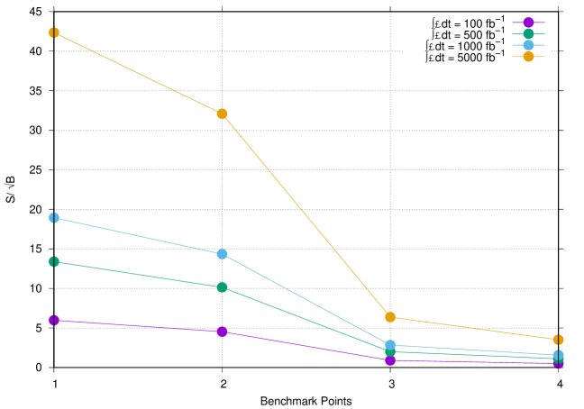
Figure 15: Signal significance corresponding to each benchmark point at integrated luminosities of $100fb^{-1}$, $500fb^{-1}$, $1000fb^{-1}$ and $5000fb^{-1}$.

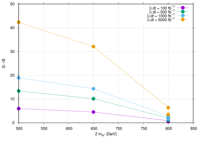
Figure 16: The Signal significance versus twice of mass of charged scalar expected for $100fb^{-1}$, $500fb^{-1}$, $1000fb^{-1}$ and $5000fb^{-1}$.

V Conclusion

In this research work, 2HDM type-I is considered as theoretical ground and scenario chosen in it is like SM in which lighter scalar Higgs (h) behaves as Standard Model Higgs boson and $\sin(\beta-\alpha)=1$. Four distinct points in the allowed region are considered and their credibility is checked by 2HDMC-1.7.0. The production and observability of charged Higgs pair $H^{\pm}$ through electron positron annihilation is investigated at four benchmark points Compact Linear Collider. The series of decays in signal process is given as $e^{+}e^{-}\rightarrow Z^{*}/\gamma^{*}\rightarrow H^{+}H^{-}\rightarrow HW^{+}HW^{-}\rightarrow jjb\overline{b}b\overline{b}jj$ in which bosonic decay of charged Higgs is considered that involves $H^{\pm}W^{\pm}H$ vertex twice in a signal process. This coupling vertex is proportional to $\sin(\beta-\alpha)$ and momenta of charged Higgs and neutral scalar Higgs bosons. As value of $\sin(\beta-\alpha)$ is set equal to unity so it is only proportional to the momentum of the particles involved.The value of $\tan\beta$ is kept relatively high to enhance the branching ratio $H\rightarrow b\overline{b}$ to benefit the signal processes.
In this work a specific bosonic decay of charged Higgs boson is considered after its production which was not studied in detail till this time. The values of all Higgs masses are taken in such a way that they permit the assumed bosonic decay kinematically. The production cross section of the signal process is determined for each benchmark point at different center of mass energies which has reasonable values which shows that this process can be used to probe the charged Higgs boson experimentally. Ignoring the minor errors, all the measurements for reconstructed charged and neutral Higgs boson invariant masses are in good agreement with their generated masses. Analysis code is run for all of assumed scenarios separately and the signal selection efficiencies are calculated for all benchmark points. The results shows that all the signals have sufficiently large total signal selection efficiencies. The reconstructed mass distributions of charged Higgs bosons and heavy Higgs bosons shows well high peaks. The analysis reveals that this process is favorable to discover the assumed scenarios for charged Higgs boson. Signal significance and total signal efficiency have been calculated for integrated luminosities at $100fb^{-1}$ and $500fb^{-1}$. The results prove that the charged Higgs is observable through pair production along with its bosonic decays. This study is supposed to provide the experimentalists a good way to examine the Higgs bosons beyond SM as well as to check the validity of 2HDM model in considered parameter space.

References

- (1) Hashemi, Majid,Charged higgs pair production in a general two higgs doublet model at and linear colliders, Commun.Theor.Phys. 61 (2014) 69.
- (2) Achard, Pablo, O. Adriani, M. Aguilar-Benitez, J. Alcaraz, G. Alemanni, J. Allaby, A. Aloisio et al., Search for charged Higgs bosons at LEP, Phys.Lett.B 575 (2003) 208-220.
- (3) Ilisie, Victor, and Antonio Pich, Low-mass fermiophobic charged Higgs phenomenology in two-Higgs-doublet models, JHEP 9 (2014) 89.
- (4) Czodrowski, Patrick, Search for Charged Higgs Bosons with the ATLAS Detector at the LHC,PhD diss., Dresden, Tech. U., (2013).
- (5) T. D. Lee,,A theory of spontaneous T violation, Phys.Rev.D8 (1973) 1226–1239.
- (6) Hashemi, Majid, and Gholamhossein Haghighat,Observability of 2HDM neutral Higgs bosons with different masses at future linear colliders, Nucl.Phys.B 951 (2020) 114903.
- (7) Ahmed, Ijaz, Sources of Charged Higgs Pair through Double or Triple Higgs Production at Linear Colliders,Advan. In HEP 2017 (2017).
- (8) CLIC, The and Charles, TK and Giansiracusa, PJ and Lucas, TG and Rassool, RP and Volpi, M and Balazs, C and Afanaciev, K and Makarenko, V and Patapenka, A and others,The Compact Linear Collider (CLIC)-2018 Summary Report,arxiv:1812.06018
- (9) Hashemi, Majid, and Gholamhossein Haghighat, Capability of future linear colliders to discover heavy neutral CP-even and CP-odd Higgs bosons within type-I 2HDM, J.Phys.G 45 (2) 095005.
- (10) Branco, Gustavo Castelo, P. M. Ferreira, L. Lavoura, M. N. Rebelo, Marc Sher, and Joao P. Silva, Theory and phenomenology of two-Higgs-doublet models, Physics reports 516 (2012) 1-102.
- (11) Arbey, A., F. Mahmoudi, O. Stål, and T. Stefaniak, Status of the charged Higgs boson in two Higgs doublet models, Eur. Phys. J.C 3 (2018) 182.
- (12) Arhrib, Abdesslam, Rachid Benbrik, Hicham Harouiz, Stefano Moretti, Yan Wang, and Qi-Shu Yan. ,Implications of light charged Higgs boson at the LHC Run III in the 2HDM., arXiv:2003.11108.
- (13) Sjöstrand, Torbjörn, Stefan Ask, Jesper R. Christiansen, Richard Corke, Nishita Desai, Philip Ilten, Stephen Mrenna, Stefan Prestel, Christine O. Rasmussen, and Peter Z. Skands. ”An introduction to PYTHIA 8.2.” Computer physics communications 191 (2015): 159-177.
- (14) D. Eriksson, J. Rathsman and O.Stal,2HDMC - Two-Higgs-Doublet Model Calculator., Comput. Phys. Commun. 181 (2010) 189.
- (15) The reference manual can be obtained at the URL: http://lcgapp.cern.ch/project/simu/HepMC/
- (16) Brun, Rene, and Fons Rademakers,ROOT—an object oriented data analysis framework, Nucl. Instrum. Meth. A 389 (1997) 81-86.
- (17) Eriksson, David, Johan Rathsman, and Oscar Stål.,2HDMC–two-Higgs-doublet model calculator, arXiv:0902.0851.
- (18) Boos, Edward, et al.,CompHEP 4.4—automatic computations from lagrangians to events, Nucl. Instrum. Meth. A 534 (2004) 250-259.
- (19) Pukhov, Alexander, et al.,,CompHEP-a package for evaluation of n diagrams and integration over multi-particle phase space, arXiv preprint hep-ph/9908288 (1999) .
- (20) Cacciari, Matteo, Gavin P. Salam, and Gregory Soyez,FastJet user manual., Eur. Phys. J.C3 (2012) 1896.
- (21) Cacciari, Matteo, Gavin P. Salam, and Gregory Soyez.,The anti-kt jet clustering algorithm,JHEP4(2008)063
- (22) Enberg, Rikard, William Klemm, Stefano Moretti, and Shoaib Munir., Electroweak production of light scalar–pseudoscalar pairs from extended Higgs sectors, Phys.Lett.B 764 (2017) 121-125.
- (23) Grimus, Walter, L. Lavoura, O. M. Ogreid, and P. Osland,A precision constraint on multi-Higgs-doublet models,J.Phys.G35(2008)075001
- (24) Yao, Wei-Ming, C. D. Amsler, David M. Asner, R. M. Bamett, J. Beringer, P. R. Burchat, C. D. Carone et al., Review of particle physics,J.Phys.G:Nuc.and part.Phys.01(2006) 001