Parameter estimation for threshold Ornstein-Uhlenbeck processes from discrete observations

Abstract

Assuming that a threshold Ornstein-Uhlenbeck process is observed at discrete time instants, we propose generalized moment estimators to estimate the parameters. Our theoretical basis is the celebrated ergodic theorem. To use this theorem we need to find the explicit form of the invariant measure. With the sampling time step $h>0$ arbitrarily fixed, we prove the strong consistency and asymptotic normality of our estimators as the sample size $N\to\infty$.

[table]capposition=top capbtabboxtable[][]

1 Introduction

Let $W=\{W(t)\}_{t\geq 0}$ be a one-dimensional standard Brownian motion on a filtered probability space $(\Omega,\mathcal{F},\mathbb{P},(\mathcal{F}_{t})_{\{t\geq 0\}})$ and let a threshold Ornstein-Uhlenbeck (hereafter abbreviated as OU) process $X$ be described by the following stochastic differential equation (SDE):

$$dX_{t}=\sum_{i=1}^{m}(\beta_{i}-\alpha_{i}X_{t})I(\theta_{i-1}<X_{t}\leq\theta_{i})dt+\sigma dW_{t},$$ (1.1)

where $\theta_{i},i=0,1,\cdots,m$ with $-\infty=\theta_{0}<\theta_{1}<\theta_{2}<\cdots<\theta_{m}=\infty$ are the so-called thresholds; $\beta_{i}\in\mathbb{R}$ and $\alpha_{i}>0$ are the drift parameters; $\sigma>0$ is the diffusion parameter; $X_{0}\in\mathbb{R}$ is a given initial condition; and $I(\cdot)$ denotes the indicator function. The existence and uniqueness of the solution to the above equation (1.1) have been known (e.g. Bass and Pardoux, 1987). Assume that the parameters $\alpha_{i}$ and $\beta_{i}$ are unknown and assume that we can observe the state $X_{t}$ of the process at discrete time instants $t_{k}=kh$, $k=1,2,\cdots,N$, where $h$ is an arbitrarily given fixed time step. This paper aims to estimate the unknown parameters $\Theta=(\alpha_{1},\cdots,\alpha_{m},\beta_{1},\cdots,\beta_{m})$ in (1.1) by using the obtained observations $\left\{X_{kh}\,,k=1,2,\cdots,N\right\}$.

The models with different levels of thresholds have been widely studied and applied in various fields. On one hand, the threshold autoregressive models are introduced to model the nonlinearities in nonlinear time series. Tong (1983) found that it is more suitable to use the threshold models to describe the asymmetry in the variance-generating mechanism. Brockwell et al. (1991), as well as, Brockwell and Hyndman (1992) investigated the problems of modelling and forecasting the continuous-time threshold process. Browne and Whitt (1995) showed that the piecewise-linear diffusion tends to be a good approximation for some birth-and-death processes. The threshold processes also played an important role in finance, we refer to the works of Chi et al. (2017), Decamps et al. (2006), Jiang et al. (2018), Siu et al. (2006), Siu (2016) and references therein. On the other hand, the threshold diffusion processes have a close tie with the skew diffusion processes that have been widely treated in financial literature (see Ding et al., 2020; Gairat and Shcherbakov, 2017; Wang et al., 2015; Zhuo and Menoukeu-Pamen, 2017; Zhuo et al., 2017).

While the threshold models are applied, an important problem is to estimate the parameters $\Theta$ through the available historical data. There have been some approaches to estimate the parameters for threshold diffusion processes such as least squares estimation, likelihood estimation, and Bayesian estimation. We refer the readers to Brockwell et al. (2007), Chan (1993), Kutoyants (2012), Lejay and Pigato (2020), and Stramer and Roberts (2007). Let us also mention that in Su and Chan (2015, 2017), the authors proposed the novel quasi-likelihood estimators and test. Within the above mentioned estimation methods, the observations are supposed to be obtained continuously. Since real data are usually collected at discrete time instants, it is necessary to estimate the parameters when only discrete observations are available. To our best knowledge, the problem to estimate parameters for a continuous-time threshold diffusion processes based on discrete observations is under-explored.

One situation in the discrete-time observations is that one has the high-frequency data, which means that in our observations $\left\{X_{kh},k=1,2,\cdots,N\right\}$, we have $h$ depends on $N$, $h\rightarrow 0$, and $Nh\rightarrow\infty$. In this case it is possible to approximate the (stochastic) integral by its “Riemann-Itô” sum to modify the continuous-time estimators to the discrete ones.

In reality, the continuous or high-frequency observations are usually impossible or very costly that we cannot have the luxury to collect such large amount of data. As a consequence, the time step $h$ must be allowed to be an arbitrarily fixed constant. Hence, we cannot borrow methods that are only valid for continuous-time observations or for high-frequency data. The present work proposes a completely different approach to address this problem. Our approach is motivated by the previous works of the construction of the estimators: the ergodic type estimators for the OU process driven by fractional Brownian motion (e.g. Hu and Song, 2013); the ergodic type estimators for the reflected OU process driven by standard Brownian motions (e.g. Hu et al., 2015); and the ergodic type estimators for the OU process driven by stable Lévy motions (e.g. Cheng et al., 2020).

Similar to the above mentioned papers, we use the ergodic theorem to obtain the generalized moment estimators for the parameters. To this end, we need first to prove the ergodic theorem for our threshold diffusion (1.1). Namely, we need to prove that there is a probability density function $\psi(x)$ such that

$$\lim_{N\rightarrow\infty}\frac{1}{N}\sum_{k=1}^{N}f(X_{t_{k}})=\int_{\mathbb{R}}f(x)\psi(x)dx$$

and we also need to find the explicit form of the probability density $\psi(x)$. This is done in Section 2. After obtaining the explicit dependence of the probability density on the parameters we let

$$\frac{1}{N}\sum_{k=1}^{N}f_{i}(X_{t_{k}})=\int_{\mathbb{R}}f_{i}(x)\psi(x)dx$$ (1.2)

for different appropriately chosen functions $f_{i}$ to obtain a suitable system of algebraic equations for the parameters. In Equation (1.1) there are $3m$ unknown parameters $\alpha_{1},\cdots,\alpha_{m},\beta_{1},\cdots,\beta_{m},{\theta}_{1},\cdots,{\theta}_{m-1},{\sigma}$. Presumably, we can choose $3m$ different functions $f$ so that we obtain a system of $3m$ equations for the $3m$ unknowns. However, some parameters are coupled with each other and cannot be separated. For example, from Remark 3.1, when $m=2$, ${\theta}_{0}=-\infty$, ${\theta}_{1}=0$, $\theta_{2}=\infty$, $\beta_{1}=\beta_{2}=0$, we see that if $(\frac{\alpha_{1}}{{\sigma}^{2}},\frac{\alpha_{2}}{{\sigma}^{2}})$ remains the same, then the invariant probability density $\psi_{1}$ remains the same function. So, even in this simplest case we cannot expect to use (1.2) to estimate $\alpha_{1}$, $\alpha_{2}$, and ${\sigma}$ simultaneously. To avoid this identifiability problem in this paper we focus on the estimation of the parameters $\Theta$ assuming ${\theta}_{1},\cdots,{\theta}_{m-1},{\sigma}$ are known. Furthermore, to better convey our idea, we focus on the case that $m=2$, ${\theta}_{0}=-\infty$, ${\theta}_{2}=\infty$, and the parameters ${\theta}={\theta}_{1}$ and ${\sigma}$ are known. This means that we shall focus on the following equation:

$$dX_{t}=(\beta_{1}-\alpha_{1}X_{t})I(X_{t}\leq\theta)dt+(\beta_{2}-\alpha_{2}X_{t})I(X_{t}>\theta)dt+\sigma dW_{t}\,,$$ (1.3)

where $\theta\in\mathbb{R}$, $\beta_{1}$, $\beta_{2}\in\mathbb{R}$, $\alpha_{1}$, $\alpha_{2}\in(0,\infty)$, and $\sigma\in(0,\infty)$. However, it should be mentioned that if ${\sigma}$ and $\theta$ are unknown, we may assume that the data are collected from the high-frequency type. In this case, ${\sigma}$ and $\theta$ can be estimated in the manners of Kutoyants (2012) and Su and Chan (2015), respectively. Now that we have four parameters ${\Theta}=(\alpha_{1},\alpha_{2},\beta_{1},\beta_{2})$, so we only need to choose four different $f$ to obtain a system of four equations. However, since the invariant probability density $\psi$ depends on the parameters in a very complex way it is hard to know whether the solution exists (locally and globally) uniquely. One of the major contributions of this work is to appropriately use the conditional moments so that we can obtain some manageable equations. This will be carried out in Section 3. We briefly summarize our efforts in that section as follows.

1. In Section 3.1, we assume $\beta_{1}=\beta_{2}={\theta}=0$. The conditional moments are introduced to obtain the explicit generalized moment estimators for $\alpha_{1}$ and $\alpha_{2}$. Furthermore, the strong consistency and asymptotic normality of the estimators are obtained.

2. In Section 3.2, we assume that $\beta_{1}=\beta_{2}=0$ whereas ${\theta}$ is known but is not equal to $0$. In this case, we can obtain two uncoupled algebraic equations for the two parameters $\alpha_{1}$ and $\alpha_{2}$ by conditional moments. Each of these equations will be shown to have a globally unique solution, yielding the generalized moment estimators for $\alpha_{1}$ and $\alpha_{2}$, although not explicitly. The strong consistency and asymptotic normality of the estimators are obtained.

3. In Section 3.3, we further assume that ${\theta}$ is known but is equal to not $0$ and we want to estimate all the four parameters $(\alpha_{1},\alpha_{2},\beta_{1},\beta_{2})$. We use the conditional moments to invert the four equations into two uncoupled systems of equations to obtain the generalized estimators for $\alpha_{1}$, $\alpha_{2}$, $\beta_{1}$, and $\beta_{2}$. The Jacobians (which are independent of data) of the two systems are computed, whose non-degeneracy implies that both systems have unique local solutions. To seek an answer for global uniqueness we reduce the problem to a simpler one of finding the zeros of two functions, both of a single variable. If the derivatives (now involving observation data) of such functions are nonzero, then the global uniqueness holds by the mean value theorem.

In our cases (2) and (3) the explicit solution to the system of algebraic equations is still hard to obtain. But there are many standard methods, such as the Newton-Raphson iteration method. It is available to solve the nonlinear system in Matlab and Mathematica by the built-in functions “fsolve” and “FindRoot”, respectively. In Section 4, some numerical experiments are provided to show the efficiency of our estimation approach. Section 5 concludes this paper.

2 Ergodicity and invariant density

Before proceeding to construct our estimators, we need some stationary and ergodic properties of the threshold diffusion process described by (1.1). The following proposition is adopted from Brockwell et al. (1991), Brockwell and Hyndman (1992), and Browne and Whitt (1995).

Proposition 2.1

Suppose that $\sigma>0$. Then the process defined by (1.1) has a stationary distribution if and only if

$$\lim_{x\to-\infty}(-\alpha_{1}x^{2}+2\beta_{1}x)<0\,,\quad\lim_{x\to\infty}(-\alpha_{m}x^{2}+2\beta_{m}x)<0\;.$$

Furthermore, the stationary density is given by

$$\psi(x)=\sum_{i=1}^{m}k_{i}\exp\left(\frac{-\alpha_{i}x^{2}+2\beta_{i}x}{\sigma^{2}}\right)I(\theta_{i-1}<x\leq\theta_{i}),$$

where $k_{i}$ are uniquely determined by the system of $m$ equations:

$$\int_{-\infty}^{\infty}\psi(x)dx=1\,,\quad{\rm and}\quad\psi(\theta_{i}-)=\psi(\theta_{i}+)\,,\quad i=1,2,\ldots,m-1\,.$$

Remark 2.2

The constants $k_{i},i=1,2,\cdots,m$ depends on the parameters in the equation (1.1). This is one of the main reasons to make the analysis of the system of algebraic equations sophisticated.

Although the stationary density function $\psi(\cdot)$ is not Gaussian, it is a mixture of Gaussian densities and has finite moments of all orders. Moreover, if the threshold OU process $X$ is stationary, it is also geometrically ergodic (see Stramer et al., 1996). The following lemma describes the stochastic stability of threshold OU processes and plays a crucial role in our estimation approach.

Lemma 2.3

The $h$-skeleton sampled chain $\{X_{kh}:k\geq 0\}$ which comes from the process $X$ defined by (1.1) is ergodic, namely, the following ergodic identity holds: for any $X_{0}\in\mathcal{S}:=\mathbb{R}$ and for any $f\in L_{1}(\mathbb{R},\psi(x)dx)$,

$$\lim_{N\to\infty}\frac{1}{N}\sum_{k=1}^{N}f(X_{kh})=\mathbb{E}[f(X_{\infty})]=\int_{\mathbb{R}}f(x)\psi(x)dx,~{}a.s.$$

Proof. It suffices to show that the process X is bounded in probability on average and is a $T$-process (see Meyn and Tweedie, 1993, Theorem 8.1). We note that the threshold diffusion process $X$ is a $\varphi$-irreducible $T$-process, where $\varphi$ is a Lebesgue measure (see Stramer et al., 1996). Moreover, since for $i=1,2$,

$$\lim_{|x|\to\infty}\left(-\alpha_{i}x^{2}+2\beta_{i}x\right)<0,$$

we have from Stramer et al. (1996, Theorem 5.1) that $X$ is a positive Harris recurrent process. Finally, by virtue of Meyn and Tweedie (1993, Theroem 3.2(ii)), we conclude that $X$ is bounded in probability on average. $\Box$

Using the same definitions as that in Karlin and Taylor (1981), the scale density function $s(x)$, scale measure $S(x)$, and speed density function $m(x)$ are given by

$$s(x)=\left\{\begin{aligned} &c_{1}\exp\left(-\frac{2\beta_{1}x}{\sigma^{2}}+\frac{\alpha_{1}x^{2}}{\sigma^{2}}\right)\;,&x\leq\theta,\\ &c_{2}\exp\left(-\frac{2\beta_{2}x}{\sigma^{2}}+\frac{\alpha_{2}x^{2}}{\sigma^{2}}\right)\;,&x>\theta,\end{aligned}\right.$$

$$S(x)=\int_{-\infty}^{x}s(y)dy,\quad m(x)=\frac{2}{s(x)\sigma^{2}},$$

where $c_{1}=\exp\left(-\frac{2\beta_{2}\theta}{\sigma^{2}}+\frac{\alpha_{2}\theta^{2}}{\sigma^{2}}\right)$ and $c_{2}=\exp\left(-\frac{2\beta_{1}\theta}{\sigma^{2}}+\frac{\alpha_{1}\theta^{2}}{\sigma^{2}}\right)$. For $i=1,2$, let

$$\widetilde{z}_{i}=\frac{\sqrt{2\alpha_{i}}}{\sigma}\left(\theta-\frac{\beta_{i}}{\alpha_{i}}\right),\quad b_{i}=\frac{\beta_{i}^{2}}{\sigma^{2}\alpha_{i}}\;.$$

Then the coefficients $k_{1}$ and $k_{2}$ of $\psi(x)$ are given by

$$k_{1} =\frac{1}{\sigma\sqrt{\pi}}\frac{\phi(\widetilde{z}_{2})}{\phi(\widetilde{z}_{2})e^{b_{1}}\Phi(\widetilde{z}_{1})/\sqrt{\alpha_{1}}+{\phi(\widetilde{z}_{1})e^{b_{1}}\Phi(-\widetilde{z}_{2})/\sqrt{\alpha_{2}}}}\;,$$ (2.4)

$$k_{2} =\frac{1}{\sigma\sqrt{\pi}}\frac{\phi(\widetilde{z}_{1})}{\phi(\widetilde{z}_{2})e^{b_{2}}\Phi(\widetilde{z}_{1})/\sqrt{\alpha_{1}}+{\phi(\widetilde{z}_{1})e^{b_{2}}\Phi(-\widetilde{z}_{2})/\sqrt{\alpha_{2}}}}\;,$$ (2.5)

where $\phi(x):=\frac{1}{\sqrt{2\pi}}e^{-x^{2}/2}$ is the normal density, $\Phi(x)=\frac{1}{\sqrt{2\pi}}\int_{-\infty}^{x}e^{-\frac{y^{2}}{2}}dy$ is the the standard normal distribution function. Although the SDE (1.3) has no explicit solution, we can derive the spectral expansion of its transition density, see the proof in A.

Proposition 2.4

For $i=1,2$, set

$$z_{i} =\frac{\sqrt{2\alpha_{i}}}{\sigma}\left(x-\frac{\beta_{i}}{\alpha_{i}}\right),\quad\nu_{i}=\frac{\lambda}{\alpha_{i}}\;,$$

$$\widetilde{z}_{i} =\frac{\sqrt{2\alpha_{i}}}{\sigma}\left(\theta-\frac{\beta_{i}}{\alpha_{i}}\right),\quad\varrho=\frac{2\beta_{1}\theta+2\beta_{2}\theta-\alpha_{1}\theta^{2}-\alpha_{2}\theta^{2}}{\sigma^{2}}.$$

Let $D_{v}(z)$ and $H_{v}(z)$ denote the parabolic cylinder function and Hermite function respectively (see Buchholz, 1969; Lebedev, 1965). Let $0\leq\lambda_{1}<\lambda_{2}<\cdots<\lambda_{n}\to\infty$ as $n\to\infty$ be the simple discrete zeros of the Wronskian equation:

$$\omega(\lambda)=\exp(\varrho)2^{1-\frac{\nu_{1}+\nu_{2}}{2}}\sigma^{-1}\left[\nu_{2}\sqrt{\alpha_{2}}H_{\nu_{1}}(-\frac{\widetilde{z}_{1}}{\sqrt{2}})H_{\nu_{2}-1}(\frac{\widetilde{z}_{2}}{\sqrt{2}})+\nu_{1}\sqrt{\alpha_{1}}H_{\nu_{2}}(\frac{\widetilde{z}_{2}}{\sqrt{2}})H_{\nu_{1}-1}(-\frac{\widetilde{z}_{1}}{\sqrt{2}})\right]=0\,.$$ (2.6)

Denote

$$\varphi_{n}(x)=\left\{\begin{aligned} &\sqrt{\frac{\eta(\theta,\lambda_{n})}{\omega^{\prime}(\lambda_{n})\xi(\theta,\lambda_{n})}}\xi(x,\lambda_{n})\;,&x\leq\theta,\\ &\operatorname{sign}(\xi(\theta,\lambda_{n})\eta(\theta,\lambda_{n}))\sqrt{\frac{\xi(\theta,\lambda_{n})}{\omega^{\prime}(\lambda)\eta(\theta,\lambda_{n})}}\eta(x,\lambda_{n})\;,&x>\theta,\end{aligned}\right.$$ (2.7)

with

$$\xi(x,\lambda)=\exp\left(z_{1}^{2}/4\right)D_{\nu_{1}}(-z_{1}),\quad\eta(x,\lambda)=\exp\left(z_{2}^{2}/4\right)D_{\nu_{2}}(z_{2})\,.$$

Then, the spectral expansion of the transition density of $X$ (defined from $\mathbb{P}(X_{t}\in A|X_{0}=x)=\int_{A}p_{t}(x,y)dy$ for any Borel set $A$ of $\mathbb{R}$) is given by

$$p_{t}(x,y)=m(y)\sum_{n=1}^{\infty}\exp(-\lambda_{n}t)\varphi_{n}(x)\varphi_{n}(y)\,.$$

3 Estimate $\alpha_{i}$ and $\beta_{i}$

In this section we attempt to construct generalized moment estimators for the parameters $\alpha=(\alpha_{1},\alpha_{2})^{T}$ and $\beta=(\beta_{1},\beta_{2})^{T}$, where $T$ denotes the transpose of a vector, and to study their strong consistency and asymptotic normality. We classify our study into several cases according to the drift parameters.

3.1 Case I: Estimate $\alpha_{i}$ for known $\beta_{i}=0$ and $\theta=0$

Here we consider the case $\beta_{i}=0$, $i=1,2$ and ${\theta}=0$. In this case the equation becomes

$$dX_{t}=-\alpha_{1}X_{t}I(X_{t}\leq 0)dt-\alpha_{2}X_{t}I(X_{t}>0)dt+\sigma dW_{t}\,.$$ (3.8)

Then the stationary density of $X$ is given by

$$\psi_{1}(x)=\frac{2\sqrt{\alpha_{1}\alpha_{2}}}{\sqrt{\pi}(\sqrt{\alpha_{1}}+\sqrt{\alpha_{2}})\sigma}\left[\exp\left(-\frac{\alpha_{1}x^{2}}{\sigma^{2}}\right)I(x\leq 0)+\exp\left(-\frac{\alpha_{2}x^{2}}{\sigma^{2}}\right)I(x>0)\right].$$ (3.9)

Remark 3.1

It is easily observed that $\psi_{1}(x)$ depends only on $\frac{\alpha_{1}}{{\sigma}^{2}}$ and $\frac{\alpha_{2}}{{\sigma}^{2}}$.

From this identity we have

Proposition 3.2

Let $X_{\infty}=\lim_{t\to\infty}X_{t}$ and define

$$L_{n}=\mathbb{E}\left[(-X_{\infty})^{n}I(X_{\infty}\leq 0)\right],\quad R_{n}=\mathbb{E}\left[X_{\infty}^{n}I(X_{\infty}>0)\right].$$

Then for any real number $n>0$,

$$L_{n} =\frac{\sigma^{n}\sqrt{\alpha_{1}\alpha_{2}}}{\alpha_{1}^{(n+1)/2}\sqrt{\pi}(\sqrt{\alpha_{1}}+\sqrt{\alpha_{2}})}\Gamma\left(\frac{n+1}{2}\right)\;,$$ (3.10)

$$R_{n} =\frac{\sigma^{n}\sqrt{\alpha_{1}\alpha_{2}}}{\alpha_{2}^{(n+1)/2}\sqrt{\pi}(\sqrt{\alpha_{1}}+\sqrt{\alpha_{2}})}\Gamma\left(\frac{n+1}{2}\right)\;,$$ (3.11)

where $\Gamma(\cdot)$ denotes the Gamma function $\Gamma(\alpha)=\int_{0}^{\infty}x^{\alpha-1}e^{-x}dx$.

From the above expressions (3.10)-(3.11) and by some elementary calculations, we can represent the parameters $\alpha_{1}$ and $\alpha_{2}$ in terms of $L_{n}$ and $R_{n}$ as

$$\alpha_{1} =\left\{\frac{\sigma^{n}\Gamma\left(\frac{n+1}{2}\right)}{\sqrt{\pi}L_{n}\left[\left(\frac{R_{n}}{L_{n}}\right)^{\frac{1}{n+1}}+1\right]}\right\}^{\frac{2}{n}},$$ (3.12)

$$\alpha_{2} =\left\{\frac{\sigma^{n}\Gamma\left(\frac{n+1}{2}\right)}{\sqrt{\pi}R_{n}\left[\left(\frac{L_{n}}{R_{n}}\right)^{\frac{1}{n+1}}+1\right]}\right\}^{\frac{2}{n}}.$$ (3.13)

Since $L_{n}>0$ and $R_{n}>0$, $\alpha_{1}$ and $\alpha_{2}$ are well-defined by (3.12) and (3.13).

Setting

$$\widehat{L}_{n,N}=\frac{1}{N}\sum_{k=1}^{N}(-X_{kh})^{n}I(X_{kh}\leq 0),\quad\widehat{R}_{n,N}=\frac{1}{N}\sum_{k=1}^{N}(X_{kh})^{n}I(X_{kh}>0),$$

we naturally construct the generalized moment estimators for $\alpha_{1},\alpha_{2}$ as follows:

$$\widehat{\alpha}_{1,n,N} =\left\{\frac{\sigma^{n}\Gamma\left(\frac{n+1}{2}\right)}{\sqrt{\pi}\widehat{L}_{n,N}\left[\left(\frac{\widehat{R}_{n,N}}{\widehat{L}_{n,N}}\right)^{\frac{1}{n+1}}+1\right]}\right\}^{\frac{2}{n}},$$ (3.14)

$$\widehat{\alpha}_{2,n,N} =\left\{\frac{\sigma^{n}\Gamma\left(\frac{n+1}{2}\right)}{\sqrt{\pi}\widehat{R}_{n,N}\left[\left(\frac{\widehat{L}_{n,N}}{\widehat{R}_{n,N}}\right)^{\frac{1}{n+1}}+1\right]}\right\}^{\frac{2}{n}}.$$ (3.15)

We will show the strong consistency and asymptotic normality of the estimators $\widehat{\alpha}_{1,n,N}$ and $\widehat{\alpha}_{2,n,N}$ of $\alpha_{1}$ and $\alpha_{2}$ in the following theorems.

Remark 3.3

Although the expectation of $(-X_{\infty})^{n}I(X_{\infty}\leq\theta)$ (or $X_{\infty}^{n}I(X_{\infty}>\theta)$) is not the $n$-th order moment in the conventional sense, it captures sufficient information about the parameters and the motivation of the estimation scheme in this paper stems from the generalized moment estimation. For this reason, we still use the term of “generalized moment estimators”.

Theorem 3.4

Fix any real number $n>0$ and fix any time step size $h>0$. Then $\widehat{\alpha}_{1,n,N}\to\alpha_{1}$ and $\widehat{\alpha}_{2,n,N}\to\alpha_{2}$ almost surely as $N\to\infty$, where $\widehat{\alpha}_{1,n,N}$, $\widehat{\alpha}_{2,n,N}$ are defined by (3.14) and (3.15) respectively.

Proof. The straightforward applications of Lemma 2.3 to $f_{1}(x)=(-x)^{n}I(x\leq 0)$ and $f_{2}(x)=x^{n}I(x>0)$ yield

$$\lim_{N\to\infty}\widehat{L}_{n,N}=L_{n}>0,\quad\lim_{N\to\infty}\widehat{R}_{n,N}=R_{n}>0,~{}a.s.$$

which imply the theorem by (3.12)-(3.15). $\Box$

Next, we study the central limit theorem (CLT) for the estimators. In comparison to Theorem 2 in Hu et al. (2015), we shall discuss the joint asymptotic normality of the estimators. Before stating our theorem we need the following notations. Denote

$$g_{1n}(x)=(-x)^{n}I(x\leq 0),\quad g_{2n}(x)=x^{n}I(x>0)\,.$$

Let $\widetilde{X}_{0}$ be a random variable with probability density function $\psi_{1}$ given by (3.9), independent of the Brownian motion and let $\widetilde{X}_{t}$ be the solution to (3.8) with initial condition $\widetilde{X}_{0}$. From Meyn and Tweedie (2009, Theorem 17.0.1), we get that

$$\sigma_{ij}^{n}:={\rm Cov}(g_{in}(\widetilde{X}_{0}),g_{jn}(\widetilde{X}_{0}))+\sum_{k=1}^{\infty}\left[{\rm Cov}(g_{in}(\widetilde{X}_{0}),g_{jn}(\widetilde{X}_{kh}))+{\rm Cov}(g_{jn}(\widetilde{X}_{0}),g_{in}(\widetilde{X}_{kh}))\right]\,,$$ (3.16)

where $i,j=1,2$, are well defined and are given by (B.40) with ${\theta}=0$. Let $G_{i,n}$, $i=1,2$ be defined on $\mathbb{R}^{2}$ by

$$G_{1,n}(x,y)=\left\{\frac{\sigma^{n}\Gamma\left(\frac{n+1}{2}\right)}{\sqrt{\pi}x\left[\left(\frac{y}{x}\right)^{\frac{1}{n+1}}+1\right]}\right\}^{\frac{2}{n}},\quad G_{2,n}(x,y)=\left\{\frac{\sigma^{n}\Gamma\left(\frac{n+1}{2}\right)}{\sqrt{\pi}y\left[\left(\frac{x}{y}\right)^{\frac{1}{n+1}}+1\right]}\right\}^{\frac{2}{n}}$$

which are the functions corresponding to (3.14) and (3.15). Denote $G_{n}=(G_{1,n},G_{2,n}):\mathbb{R}^{2}\to\mathbb{R}^{2}$.

Now we can state our main result of this subsection.

Theorem 3.5

Fix an arbitrary $h>0$. Denote $\alpha=(\alpha_{1},\alpha_{2})^{T}$ and $\widehat{\alpha}_{n,N}=(\widehat{\alpha}_{1,n,N},\widehat{\alpha}_{2,n,N})^{T}$, where $\widehat{\alpha}_{1,n,N}$, $\widehat{\alpha}_{2,n,N}$ are defined by (3.14) and (3.15) respectively. Then as $N\to\infty$,

$$\sqrt{N}\left(\widehat{\alpha}_{n,N}-\alpha\right) \Rightarrow\mathbf{N}\left(0,\nabla G_{n}(L_{n},R_{n})\cdot\Sigma_{n}\cdot\nabla G_{n}(L_{n},R_{n})^{T}\right)\,,$$

where the symbol “$\Rightarrow$” denotes convergence in distribution, $\mathbf{N}(\mu,\Sigma)$ stands for the normal random vector with mean $\mu$ and variance $\Sigma$, and $\Sigma_{n}:=(\sigma_{ij}^{n})_{1\leq i,j\leq 2}$ with $\sigma_{ij}^{n}$ being defined by (3.16) or equivalently by (B.40) with ${\theta}=0$ .

Proof. The proof is carried out in two steps. First, we establish the bivariate CLT for $(\widehat{L}_{n,N},\widehat{R}_{n,N})^{T}$, then we employ the bivariate delta method. Recall that $\{X_{kh}\}$ is a positive Harris chain with invariant probability $\psi$ (Lemma 2.3) and is $V$-uniformly ergodic with a function $V(x)=x^{2m}+1$ or $V(x)=e^{x^{2m}}+1$ (see Stramer et al., 1996, Theorem 5.1). That is to say, there exist $R\in(0,\infty)$ and $\rho\in(0,1)$ such that for all $x\in\mathbb{R}$,

$$||P^{n}(x,\cdot)-\psi_{1}||_{V}\leq RV(x)\rho^{n},$$

where $V$-norm $||\nu||_{V}:=\sup_{g:g\leq V}|\nu(g)|$, $\nu$ is any signed measure (see Meyn and Tweedie, 2009, Page 334), and $P^{n}(x,B):=P_{nh}(x,B):=\mathbb{P}(X_{nh}\in B)$ is an $n$-step transition probability function of the sampled chain $\{X_{kh}\}_{k\geq 0}$ from the initial point $x$ to set $B$. Then from Meyn and Tweedie (2009, Theorem 17.0.1), for any $(a_{1},a_{2})\in\mathbb{R}^{2}$, letting $A(x)=a_{1}x^{n}I(x\leq 0)+a_{2}x^{n}I(x>0)$, we know that

$$\sqrt{N}(a_{1}\widehat{L}_{n,N}+a_{2}\widehat{R}_{n,N})=\frac{1}{\sqrt{N}}\sum_{k=1}^{N}A(X_{kh})=:\frac{1}{\sqrt{N}}S_{n}(A)$$

converges to some normal random variable $Z_{a_{1},a_{2}}$ in the sense of distribution. By the Cramér-Wold device we know that $\sqrt{N}(\widehat{L}_{n,N},\widehat{R}_{n,N})^{T}$ converges jointly to a (two-dimensional) normal vector. Moreover, in view of the multivariable Markov chain CLT (Brooks et al., 2011, Section 1.8.1), we have

$$\sqrt{N}((\widehat{L}_{n,N},\widehat{R}_{n,N})^{T}-(L_{n,N},R_{n,N})^{T})\Rightarrow\mathbf{N}(0,\Sigma_{n})\,,$$

where $\sigma_{ij}^{n}$ is defined by (3.16). Let us recall the sufficient conditions of the multivariate delta method (see van der Vaart, 1998): all partial derivatives $\partial G_{j}(x,y)/\partial x$ and $\partial G_{j}(x,y)/\partial y$ exist for $(x,y)$ in a neighborhood of $(L_{n},R_{n})$ (notice that $L_{n}>0$ and $R_{n}>0$) and are continuous at $(L_{n},R_{n})$. It is clear that the conditions are justified. From the multivariate delta method, the following desired result follows

$$\sqrt{N}\left(G_{n}(\widehat{L}_{n,N},\widehat{R}_{n,N})-G_{n}(L_{n},R_{n})\right)\Rightarrow\mathbf{N}\left(0,\nabla G_{n}(L_{n},R_{n})\cdot\Sigma_{n}\cdot\nabla G_{n}(L_{n},R_{n})^{T}\right).$$

Hence, we complete the proof. $\Box$

Remark 3.6

The asymptotic variance is given by $\nabla G_{n}(L_{n},R_{n})\cdot\Sigma_{n}\cdot\nabla G_{n}(L_{n},R_{n})^{T}$. Our numerical experiments show that the estimators perform better when $\alpha_{1}$ and $\alpha_{2}$ are smaller in terms of mean squared error (MSE), see Figure 1, where we set $\sigma=1$, $h=0.5$, $N=100,000$. From Figure 1 , we also see that the best estimators is to choose the moment $n$ to be between $2$ and $4$.

(a) $\widehat{\alpha}_{1,n,N}$ against $n$ ($\alpha_{1}=0.02$)

(b) $\widehat{\alpha}_{2,n,N}$ against $n$ ($\alpha_{1}=0.05$)

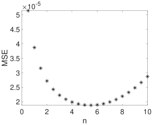
(c) $\widehat{\alpha}_{1,n,N}$ against $n$ ($\alpha_{1}=0.1$)

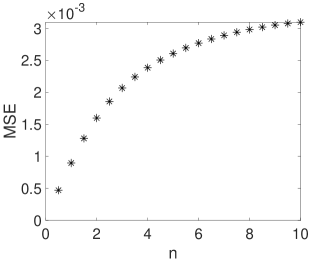
(d) $\widehat{\alpha}_{2,n,N}$ against $n$ ($\alpha_{1}=0.5$)

Figure 1: MSE of $\widehat{\alpha}_{1,n,N}$ and $\widehat{\alpha}_{2,n,N}$.

3.2 Case II: Estimate $\alpha_{i}$ for known $\beta_{i}=0$ and $\theta\neq 0$

Now we consider the case $\theta\neq 0$, $\beta_{i}=0$, $i=1,2$. Recall the explicit expression for the stationary density we obtained in Section 2:

$$\psi_{2}(x)=k_{1}\exp\left(-\frac{\alpha_{1}x^{2}}{\sigma^{2}}\right)I(x\leq\theta)+k_{2}\exp\left(-\frac{\alpha_{2}x^{2}}{\sigma^{2}}\right)I(x>\theta),$$

where $k_{1}$ and $k_{2}$ are determined by $\psi_{2}(\theta-)=\psi_{2}(\theta+)$ and $\int_{-\infty}^{\infty}\psi_{2}(x)dx=1$. The constants $k_{1}$ and $k_{2}$ are complicated functions of the unknown parameters $\alpha_{1}$ and $\alpha_{2}$. We shall use the technique of conditional moments to get rid of them. Since the stationary distribution of $X$ is Gaussian conditioned to stay in the interval $(-\infty,\theta)$ or the interval $(\theta,\infty)$, we shall focus on the conditional moments of $X_{\infty}$. Some elementary calculations give

$$\left\{\begin{aligned} &\mathbb{E}[X_{\infty}|X_{\infty}\leq\theta]=\frac{\mathbb{E}[X_{\infty}I(X_{\infty}\leq\theta)]}{\mathbb{E}[I(X_{\infty}\leq\theta)]}=-\frac{\sigma}{\sqrt{2\alpha_{1}}}\frac{\phi(-\sqrt{2\alpha_{1}}\theta/\sigma)}{1-\Phi(-\sqrt{2\alpha_{1}}\theta/\sigma)},\\ &\mathbb{E}[X_{\infty}|X_{\infty}>\theta]=\frac{\mathbb{E}[X_{\infty}I(X_{\infty}>\theta)]}{\mathbb{E}[I(X_{\infty}>\theta)]}=\frac{\sigma}{\sqrt{2\alpha_{2}}}\frac{\phi(\sqrt{2\alpha_{2}}\theta/\sigma)}{1-\Phi(\sqrt{2\alpha_{2}}\theta/\sigma)}\,.\end{aligned}\right.$$

For simplicity of notations, we set

$$\widehat{L}_{n,N}^{\theta}=\frac{1}{N}\sum_{k=1}^{N}X_{kh}^{n}I(X_{kh}\leq\theta),\quad\widehat{R}_{n,N}^{\theta}=\frac{1}{N}\sum_{k=1}^{N}X_{kh}^{n}I(X_{kh}>\theta),$$ (3.17)

$$L_{n}^{\theta}=\mathbb{E}[X_{\infty}^{n}I(X_{\infty}\leq\theta)],\quad R_{n}^{\theta}=\mathbb{E}[X_{\infty}^{n}I(X_{\infty}>\theta)].$$ (3.18)

Motivated from the approximations $\widehat{L}_{n,N}^{\theta}\approx L_{n}^{\theta}$ and $\widehat{R}_{n,N}^{\theta}\approx R_{n}^{\theta}$, we use the following equations to construct our estimators for the parameters $\alpha_{1},\alpha_{2}$:

$$\left\{\begin{aligned} &\frac{\widehat{L}_{1,N}^{\theta}}{\widehat{L}_{0,N}^{\theta}}=-\frac{\sigma}{\sqrt{2\alpha_{1}}}\frac{\phi(-\sqrt{2\alpha_{1}}\theta/\sigma)}{1-\Phi(-\sqrt{2\alpha_{1}}\theta/\sigma)},\\ &\frac{\widehat{R}_{1,N}^{\theta}}{\widehat{R}_{0,N}^{\theta}}=\frac{\sigma}{\sqrt{2\alpha_{2}}}\frac{\phi(\sqrt{2\alpha_{2}}\theta/\sigma)}{1-\Phi(\sqrt{2\alpha_{2}}\theta/\sigma)}.\end{aligned}\right.$$ (3.19)

Let

$$x=\frac{\sqrt{2\alpha_{1}}\theta}{\sigma}\,,\qquad y=\frac{\sqrt{2\alpha_{2}}\theta}{\sigma}\,,$$ (3.20)

and

$$A(x)=\frac{\phi(-x)}{1-\Phi(-x)},\quad B(y)=\frac{\phi(y)}{1-\Phi(y)}.$$

Equivalently, the system of equations (3.19) becomes

$$\left\{\begin{aligned} &\frac{\widehat{L}_{1,N}^{\theta}}{\theta\widehat{L}_{0,N}^{\theta}}=-\frac{A(x)}{x}=:K_{1}(x),\\ &\frac{\widehat{R}_{1,N}^{\theta}}{\theta\widehat{R}_{0,N}^{\theta}}=\frac{B(y)}{y}=:K_{2}(y).\end{aligned}\right.$$ (3.21)

These are two uncoupled equations, so we can solve them separately. To see if there is a unique solution to each of the above equations or not, we use the simple mean value theorem: if a differentiable function $f$ has nonzero derivatives on an interval $I$, then it is injective. Using the fact that $A^{\prime}(x)=-xA(x)-A^{2}(x)$ and $B^{\prime}(y)=-yB(y)+B^{2}(y)$, we can compute the derivatives of $K_{1}$ and $K_{2}$ as follows:

$$\left\{\begin{aligned} &\frac{dK_{1}}{dx}=A(x)\left(\frac{1}{x^{2}}+1+\frac{A(x)}{x}\right),\\ &\frac{dK_{2}}{dy}=-B(y)\left(\frac{1}{y^{2}}+1-\frac{B(y)}{y}\right).\end{aligned}\right.$$

To investigate the monotonicity of $K_{i}$, $i=1,2$, it is equivalent to show the positivity or negativity of $F_{1}(x)=\frac{1}{x^{2}}+1+\frac{A}{x}$ and $F_{2}(y):=\frac{1}{y^{2}}+1-\frac{B}{y}$. Since $F_{1}(-y)=F_{2}(y)$, to show each of the equation in (3.21) has a unique solution in $\mathbb{R}$, we only need to show $F_{1}(x)>0$ for all $x\neq 0$. Denote $\widetilde{F}(x):=1-\Phi(-x)+x^{2}(1-\Phi(-x))+x\phi(-x)$. Then $F_{1}(x)=\widetilde{F}(x)/[x^{2}(1-\Phi(-x))]$. Note that

$$\widetilde{F}^{\prime}(x)=2\phi(x)+2x\Phi(x),\quad\widetilde{F}^{\prime\prime}(x)=2\Phi(x)>0.$$

Since $\lim_{x\to-\infty}\widetilde{F}^{\prime}(x)=0$, we see $\widetilde{F}^{\prime}(x)>0$. Now we can conclude that $\widetilde{F}(x)>0$ from $\lim_{x\to-\infty}\widetilde{F}(x)=0$. Therefore, there exists a continuous inverse function $H=(H_{1},H_{2})$ of $(K_{1},K_{2})$ such that

$$\widehat{x}_{N}:=H_{1}\left(\frac{\widehat{L}_{1,N}^{\theta}}{{\theta}\widehat{L}_{0,N}^{\theta}}\right),\quad\widehat{y}_{N}:=H_{2}\left(\frac{\widehat{R}_{1,N}^{\theta}}{{\theta}\widehat{R}_{0,N}^{\theta}}\right).$$

From the ergodic theorem we know that $\widehat{L}_{n,N}^{\theta}$ and $\widehat{R}_{n,N}^{\theta}$ converge almost surely to $L_{n}^{\theta}$ and $R_{n}^{\theta}$ defined by (3.18). Thus, the estimators $\widehat{x}_{N}$ and $\widehat{y}_{N}$ converge almost surely to the parameters

$$x=H_{1}(K_{1}(x))=\frac{\sqrt{2\alpha_{1}}\theta}{\sigma},\quad y=H_{2}(K_{2}(y))=\frac{\sqrt{2\alpha_{2}}\theta}{\sigma}$$ (3.22)

respectively, as $N\to\infty$. Now the relationship (3.20) between $(x,y)$ and $(\alpha_{1},\alpha_{2})$ yields the following theorem.

Theorem 3.7

For any sample size $N$ the system of equations (3.21) has a unique solution $(\widehat{x}_{N},\widehat{y}_{N})$. The generalized moment estimators defined by

$$\widehat{\alpha}_{1,N}=\frac{1}{2}\left(\frac{\sigma\widehat{x}_{N}}{\theta}\right)^{2},\quad\widehat{\alpha}_{2,N}=\frac{1}{2}\left(\frac{\sigma\widehat{y}_{N}}{\theta}\right)^{2}$$

are strongly consistent, namely, $(\widehat{\alpha}_{1,N},\widehat{\alpha}_{2,N})$ converges to $(\alpha_{1},\alpha_{2})$ almost surely.

Compared with the case I, the estimators only have implicit expressions in terms of the inverse functions $H_{1}$ and $H_{2}$. Nevertheless, it is clear that $H_{1}$ and $H_{2}$ are continuously differentiable. Hence, we can exhibit the following CLT for the estimators $\widehat{\alpha}_{i,N}$, $i=1,2$.

Theorem 3.8

As $N\to\infty$,

$$\sqrt{N}\left((\widehat{\alpha}_{1,N},\widehat{\alpha}_{2,N})^{T}-(\alpha_{1},\alpha_{2})^{T}\right)\Rightarrow\mathbf{N}(0,\widehat{\Sigma}),$$

where $\widehat{\Sigma}$ is given by (3.23) below.

Proof. The proof is similar to that of Theorem 3.5, so we only provide a sketch of the proof. Set

$$F_{1}(x)=I(x\leq\theta),\quad F_{2}(x)=xI(x\leq\theta)\,,$$

$$F_{3}(x)=I(x>\theta),\quad F_{4}(x)=xI(x>\theta)\,.$$

From Meyn and Tweedie (2009, Theorem 17.0.1), we get that for $i,j=1,2,3,4,$

$$\widetilde{\sigma}_{ij}:={\rm Cov}(F_{i}(\widetilde{X}_{0}),F_{j}(\widetilde{X}_{0}))+\sum_{k=1}^{\infty}\left[{\rm Cov}(F_{i}(\widetilde{X}_{0}),F_{j}(\widetilde{X}_{kh}))+{\rm Cov}(F_{j}(\widetilde{X}_{0}),F_{i}(\widetilde{X}_{kh}))\right],$$

are well defined and non-negative. They can be computed by using (B.40) as follows:

$$\tilde{\sigma}_{ij}=\sigma(F_{i},F_{j})\,,\quad i,j=1,2,3,4\,.$$

Denote $\tilde{\Sigma}_{2}:=(\tilde{\sigma}_{ij})_{1\leq i,j\leq 4}$, then we have

$$\sqrt{N}\left((\widehat{L}_{0,N}^{\theta},\widehat{L}_{1,N}^{\theta},\widehat{R}_{0,N}^{\theta},\widehat{R}_{1,N}^{\theta})^{T}-(L_{0}^{\theta},L_{1}^{\theta},R_{0}^{\theta},R_{1}^{\theta})^{T}\right)\Rightarrow\mathbf{N}(0,\tilde{\Sigma}_{2}).$$

Define two functions by $h_{1}(x_{1},x_{2}):=H_{1}(\frac{x_{2}}{\theta x_{1}})$ and $h_{2}(x_{3},x_{4}):=H_{2}(\frac{x_{4}}{\theta x_{3}})$ and set two maps

$$h:(x_{1},x_{2},x_{3},x_{4})\mapsto(h_{1}(x_{1},x_{2}),h_{2}(x_{3},x_{4}))\;,$$

$$l:(x_{1},x_{2})\mapsto\left(\frac{\sigma^{2}{x_{1}}^{2}}{2\theta^{2}},\frac{\sigma^{2}{x_{2}}^{2}}{2\theta^{2}}\right)\;.$$

By the multivariate delta method, we have

$$\sqrt{N}\left(h(\widehat{L}_{0,N}^{\theta},\widehat{L}_{1,N}^{\theta},\widehat{R}_{0,N}^{\theta},\widehat{R}_{1,N}^{\theta})^{T}-h(L_{0}^{\theta},L_{1}^{\theta},R_{0}^{\theta},R_{1}^{\theta})^{T}\right)\Rightarrow\mathbf{N}(0,\bar{\Sigma}),$$

where $\bar{\Sigma}=\nabla h(L_{0}^{\theta},L_{1}^{\theta},R_{0}^{\theta},R_{1}^{\theta})\tilde{\Sigma}_{2}\nabla h(L_{0}^{\theta},L_{1}^{\theta},R_{0}^{\theta},R_{1}^{\theta})^{T}$. Applying the multivariate delta method again, we get the desired CLT result

$$\sqrt{N}\left(l(h(\widehat{L}_{0,N}^{\theta},\widehat{L}_{1,N}^{\theta},\widehat{R}_{0,N}^{\theta},\widehat{R}_{1,N}^{\theta}))^{T}-l(h(L_{0}^{\theta},L_{1}^{\theta},R_{0}^{\theta},R_{1}^{\theta}))^{T}\right)\Rightarrow\mathbf{N}(0,\widehat{\Sigma}),$$

where

$$\widehat{\Sigma}:=\nabla l(h(L_{0}^{\theta},L_{1}^{\theta},R_{0}^{\theta},R_{1}^{\theta}))\ \bar{\Sigma}\ \nabla l(h(L_{0}^{\theta},L_{1}^{\theta},R_{0}^{\theta},R_{1}^{\theta}))^{T}\,.$$ (3.23)

The proof is then completed. $\Box$

3.3 Case III: Estimate $\beta_{i}$ and $\alpha_{i}$ for known $\theta\neq 0$

In this subsection, we extend our approach to multiple-parameter case, where $\theta\neq 0$. The stationary density is given by

$$\psi_{3}(x)=k_{1}\exp\left(\frac{-\alpha_{1}x^{2}+2\beta_{1}x}{\sigma^{2}}\right)I(x\leq\theta)+k_{2}\exp\left(\frac{-\alpha_{2}x^{2}+2\beta_{2}x}{\sigma^{2}}\right)I(x>\theta),$$ (3.24)

where $k_{1}$ and $k_{2}$ are defined by (2.4) and (2.5). We can obtain the following stationary moments

$$\left\{\begin{aligned} &\frac{\mathbb{E}[X_{\infty}I(X_{\infty}\leq\theta)]}{\mathbb{E}[I(X_{\infty}\leq\theta)]}=\frac{-\frac{\sigma}{\sqrt{2\alpha_{1}}}\phi\left(\frac{\sqrt{2\alpha_{1}}\theta}{\sigma}-\frac{2\beta_{1}}{\sqrt{2\alpha_{1}}\sigma}\right)}{\Phi\left(\frac{\sqrt{2\alpha_{1}}\theta}{\sigma}-\frac{2\beta_{1}}{\sqrt{2\alpha_{1}}\sigma}\right)}+\frac{\beta_{1}}{\alpha_{1}},\\ &\frac{\mathbb{E}[X_{\infty}^{2}I(X_{\infty}\leq\theta)]}{\mathbb{E}[I(X_{\infty}\leq\theta)]}=\frac{\sigma^{2}}{2\alpha_{1}}+\left(\frac{\beta_{1}}{\alpha_{1}}\right)^{2}+\frac{\phi\left(\frac{\sqrt{2\alpha_{1}}\theta}{\sigma}-\frac{2\beta_{1}}{\sqrt{2\alpha_{1}}\sigma}\right)}{\Phi\left(\frac{\sqrt{2\alpha_{1}}\theta}{\sigma}-\frac{2\beta_{1}}{\sqrt{2\alpha_{1}}\sigma}\right)}\left(-\theta-\frac{\beta_{1}}{\alpha_{1}}\right)\frac{\sigma}{\sqrt{2\alpha_{1}}}\,,\\ &\frac{\mathbb{E}[X_{\infty}I(X_{\infty}>\theta)]}{\mathbb{E}[I(X_{\infty}>\theta)]}=\frac{\frac{\sigma}{\sqrt{2\alpha_{2}}}\phi\left(\frac{\sqrt{2\alpha_{2}}\theta}{\sigma}-\frac{2\beta_{2}}{\sqrt{2\alpha_{2}}\sigma}\right)}{1-\Phi\left(\frac{\sqrt{2\alpha_{2}}\theta}{\sigma}-\frac{2\beta_{2}}{\sqrt{2\alpha_{2}}\sigma}\right)}+\frac{\beta_{2}}{\alpha_{2}},\\ &\frac{\mathbb{E}[X_{\infty}^{2}I(X_{\infty}>\theta)]}{\mathbb{E}[I(X_{\infty}>\theta)]}=\frac{\sigma^{2}}{2\alpha_{2}}+\left(\frac{\beta_{2}}{\alpha_{2}}\right)^{2}+\frac{\phi\left(\frac{\sqrt{2\alpha_{1}}\theta}{\sigma}-\frac{2\beta_{1}}{\sqrt{2\alpha_{1}}\sigma}\right)}{1-\Phi\left(\frac{\sqrt{2\alpha_{1}}\theta}{\sigma}-\frac{2\beta_{1}}{\sqrt{2\alpha_{1}}\sigma}\right)}\left(\theta+\frac{\beta_{1}}{\alpha_{1}}\right)\frac{\sigma}{\sqrt{2\alpha_{2}}}\,.\end{aligned}\right.$$ (3.25)

Denote the right-hand sides of the above identities by $\bar{K}_{i}$, $i=1,2,3,4$. Let

$$v =\frac{\beta_{1}}{\alpha_{1}},\quad u=\frac{\sqrt{2\alpha_{1}}\theta}{\sigma}-\frac{2\beta_{1}}{\sqrt{2\alpha_{1}}\sigma}=\frac{\sqrt{2\alpha_{1}}(\theta-v)}{\sigma},\quad A(u)=\frac{\phi(-u)}{1-\Phi(-u)},$$ (3.26)

$$z =\frac{\beta_{2}}{\alpha_{2}},\quad\omega=\frac{\sqrt{2\alpha_{2}}\theta}{\sigma}-\frac{2\beta_{2}}{\sqrt{2\alpha_{2}}\sigma}=\frac{\sqrt{2\alpha_{2}}(\theta-z)}{\sigma},\quad B(\omega)=\frac{\phi(\omega)}{1-\Phi(\omega)}\,.$$ (3.27)

Then we can rewrite $\bar{K}_{i}$ as

$$\left\{\begin{aligned} &\bar{K}_{1}(u,v)=\frac{v-\theta}{u}A(u)+v,\\ &\bar{K}_{2}(u,v)=\left(\frac{\theta-v}{u}\right)^{2}+v^{2}-A(u)\frac{\theta^{2}-v^{2}}{u}\,,\\ &\bar{K}_{3}(\omega,z)=\frac{\theta-z}{\omega}B(\omega)+z,\\ &\bar{K}_{4}(\omega,z)=\left(\frac{\theta-z}{\omega}\right)^{2}+z^{2}+B(\omega)\frac{\theta^{2}-z^{2}}{\omega}\,.\end{aligned}\right.$$ (3.28)

Similar to the previous cases, we approximate the left hand sides of (3.25) by the following statistics for $i=1,2$:

$$\widehat{L}_{i,N}^{\theta}/\widehat{L}_{0,N}^{\theta} \approx\mathbb{E}[(X_{\infty})^{i}I(X_{\infty}\leq\theta)]/\mathbb{E}[I(X_{\infty}\leq\theta)],$$

$$\widehat{R}_{i,N}^{\theta}/\widehat{R}_{0,N}^{\theta} \approx\mathbb{E}[(X_{\infty})^{i}I(X_{\infty}\leq\theta)]/\mathbb{E}[I(X_{\infty}>\theta)],$$

Motivated by (3.25) and (3.28) we first propose the following estimators $\widehat{v}_{N}$, $\widehat{u}_{N}$, $\widehat{z}_{N}$, and $\widehat{\omega}_{N}$ to estimate $v,u,z,\omega$ by solving the following system

$$\left\{\begin{aligned} &\frac{\widehat{L}_{1,N}^{\theta}}{\widehat{L}_{0,N}^{\theta}}=\frac{v-\theta}{u}A(u)+v,\\ &\frac{\widehat{L}_{2,N}^{\theta}}{\widehat{L}_{0,N}^{\theta}}=\left(\frac{\theta-v}{u}\right)^{2}+v^{2}-A(u)\frac{\theta^{2}-v^{2}}{u}\,,\\ &\frac{\widehat{R}_{1,N}^{\theta}}{\widehat{R}_{0,N}^{\theta}}=\frac{\theta-z}{\omega}B(\omega)+z,\\ &\frac{\widehat{R}_{2,N}^{\theta}}{\widehat{R}_{0,N}^{\theta}}=\left(\frac{\theta-z}{\omega}\right)^{2}+z^{2}+B(\omega)\frac{\theta^{2}-z^{2}}{\omega}\,.\end{aligned}\right.$$ (3.29)

Next we need to solve this system of four equations. First, we observe that this system of four equations is decoupled as two systems, each consisting two equations. Let us first study the first pair of equations in (3.29):

$$\left\{\begin{aligned} &\frac{\widehat{L}_{1,N}^{\theta}}{\widehat{L}_{0,N}^{\theta}}=\frac{v-\theta}{u}A(u)+v=:\bar{K}_{1}(u,v)\,,\\ &\frac{\widehat{L}_{2,N}^{\theta}}{\widehat{L}_{0,N}^{\theta}}=\left(\frac{\theta-v}{u}\right)^{2}+v^{2}-A(u)\frac{\theta^{2}-v^{2}}{u}=:\bar{K}_{2}(u,v)\,.\end{aligned}\right.$$ (3.30)

The partial derivatives of $\bar{K}_{1},\bar{K}_{2}$ are given by

$$\left\{\begin{aligned} &\frac{\partial\bar{K}_{1}}{\partial u}=-\frac{v-\theta}{u^{2}}A(u)-(v-\theta)A(u)-A^{2}(u)\frac{v-\theta}{u}\,,\\ &\frac{\partial\bar{K}_{1}}{\partial v}=\frac{A(u)}{u}+1\,,\\ &\frac{\partial\bar{K}_{2}}{\partial u}=-\frac{2(\theta-v)^{2}}{u^{3}}-(-uA(u)-A^{2}(u))\frac{\theta^{2}-v^{2}}{u}+A(u)\frac{\theta^{2}-v^{2}}{u^{2}}\,,\\ &\frac{\partial\bar{K}_{2}}{\partial v}=-\frac{2(\theta-v)}{u^{2}}+2v+\frac{2A(u)v}{u}\,.\end{aligned}\right.$$

The Jacobian matrix $J_{1}$ of $(\bar{K}_{1},\bar{K}_{2})$ is given by

$$J_{1}=\begin{pmatrix}\frac{\partial\bar{K}_{1}}{\partial u}&\frac{\partial\bar{K}_{1}}{\partial v}\\ \frac{\partial\bar{K}_{2}}{\partial u}&\frac{\partial\bar{K}_{2}}{\partial v}\\ \end{pmatrix}.$$

The determinant of $J_{1}$ is

$$\det(J_{1})=-\frac{(v-\theta)^{2}}{u^{3}}(A(u)u^{3}+3A(u)u+A^{3}(u)u+2A^{2}(u)u^{2}+3A^{2}(u)-2)\;.$$

Let $D_{1}(u)=A(u)u^{3}+3A(u)u+A^{3}(u)u+2A^{2}(u)u^{2}+3A^{2}(u)-2$. To show that $\det(J_{1})\neq 0$ for all $u\neq 0$ and $v\neq\theta$ it suffices to show that $D_{1}(u)<0$. From the Figure 2, we can see that $D_{1}(u)<0$ for all $u\in[-10,5]$. Let

$$\mathbb{D}_{1} = \left\{(u,v)\in\mathbb{R}^{2}\,;v\not=\theta\,\right.\ {\rm and}$$

$$\left.D_{1}(u)=A(u)u^{3}+3A(u)u+A^{3}(u)u+2A^{2}(u)u^{2}+3A^{2}(u)-2\not=0\right\}\,.$$

The Figure 2 implies $\left\{(u,v),u\in(-10,5)\,,v\not=0\right\}\subseteq\mathbb{D}_{1}$. If necessary, one can enlarge the interval $(-10,5)$. If $(u_{0},v_{0})\in\mathbb{D}_{1}$ is from the true parameters $(\alpha_{1},\beta_{1})$, then by the ergodic Lemma 2.3 we know that when $N$ goes to infinity (3.30) will become true identities with the $(u,v)$ on the right-hand side replaced by $(u_{0},v_{0})$. Thus, when $N$ is sufficiently large $\displaystyle\left(\frac{\widehat{L}_{1,N}^{\theta}}{\widehat{L}_{0,N}^{\theta}}\,,\frac{\widehat{L}_{2,N}^{\theta}}{\widehat{L}_{0,N}^{\theta}}\right)$ will be in any given neighbourhood of $(\bar{K}_{1}(u_{0},v_{0}),\bar{K}_{2}(u_{0},v_{0}))$. On the other hand, it is obvious that $\mathbb{D}_{1}$ is an open set in $\mathbb{R}^{2}$ and $\bar{K}_{1},\bar{K}_{2}$ are continuous functions of $(u,v)$. Since $\det(J_{1})\not=0$ on $\mathbb{D}_{1}$, by the inverse function theorem there is one unique solution pair $(u,v)\in\mathbb{D}_{1}$ in some neighbourhood of $(u_{0},v_{0})$ such that the system of equations (3.30) are satisfied. This gives the existence and local uniqueness of the solution to the system of equations (3.30).

Now we consider the second pair of equations in (3.29).

$$\left\{\begin{aligned} &\frac{\widehat{R}_{1,N}^{\theta}}{\widehat{R}_{0,N}^{\theta}}=\frac{\theta-z}{\omega}B(\omega)+z=:\bar{K}_{3}(\omega,z)\,,\\ &\frac{\widehat{R}_{2,N}^{\theta}}{\widehat{R}_{0,N}^{\theta}}=\left(\frac{\theta-z}{\omega}\right)^{2}+z^{2}+B(\omega)\frac{\theta^{2}-z^{2}}{\omega}=:\bar{K}_{4}(\omega,z)\,.\end{aligned}\right.$$ (3.31)

The partial derivatives of $\bar{K}_{3}(\omega,z)$, $\bar{K}_{4}(\omega,z)$ are

$$\left\{\begin{aligned} &\frac{\partial\bar{K}_{3}}{\partial\omega}=-\frac{\theta-z}{\omega^{2}}B(\omega)-(\theta-z)B(\omega)+B^{2}(\omega)\frac{\theta-z}{\omega}\\ &\frac{\partial\bar{K}_{3}}{\partial z}=-\frac{B(\omega)}{\omega}+1,\\ &\frac{\partial\bar{K}_{4}}{\partial\omega}=-\frac{2(\theta-z)^{2}}{\omega^{3}}+(-\omega B(\omega)+B^{2}(\omega))\frac{\theta^{2}-z^{2}}{\omega}-B(\omega)\frac{\theta^{2}-z^{2}}{\omega^{2}},\\ &\frac{\partial\bar{K}_{4}}{\partial z}=-\frac{2(\theta-z)}{\omega^{2}}+2z-\frac{2B(\omega)z}{\omega}\\ \end{aligned}\right.$$

The determinant of the Jacobian matrix $J_{2}$ of $(\bar{K}_{3},\bar{K}_{4})$ is

$$\det(J_{2})=\frac{(\theta-z)^{2}}{\omega^{3}}(B(\omega)\omega^{3}+3B(\omega)\omega+B^{3}(\omega)\omega-2B^{2}(\omega)\omega^{2}-3B^{2}(\omega)-2)\;.$$

Let $D_{2}(\omega)=B(\omega)\omega^{3}+3B(\omega)\omega+B^{3}(\omega)\omega-2B^{2}(\omega)\omega^{2}-3B^{2}(\omega)-2$. From the Figure 3, we see that $D_{2}(\omega)<0$ for all $\omega\in[-5,5]$. Denote

$$\mathbb{D}_{2} = \left\{(z,\omega)\in\mathbb{R}^{2}\,;z\not=\theta\,\right.\ {\rm and}$$

$$\left.D_{2}(\omega)=B(\omega)\omega^{3}+3B(\omega)\omega+B^{3}(\omega)\omega-2B^{2}(\omega)\omega^{2}-3B^{2}(\omega)-2\not=0\right\}\,.$$

Analogous to the argument for the system of equations (3.30) we can prove the existence and local uniqueness of the solution to the system of equations (3.31).

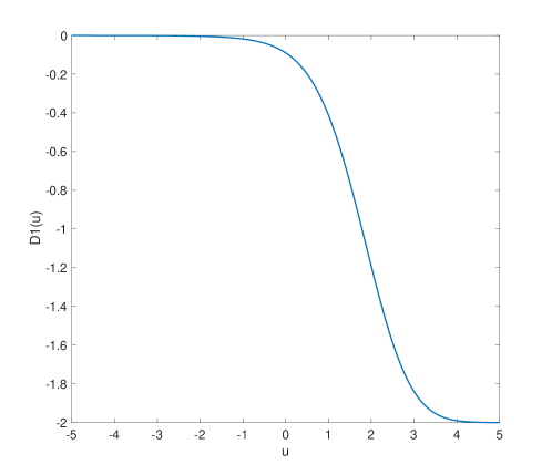
(a) $D_{1}(u)$

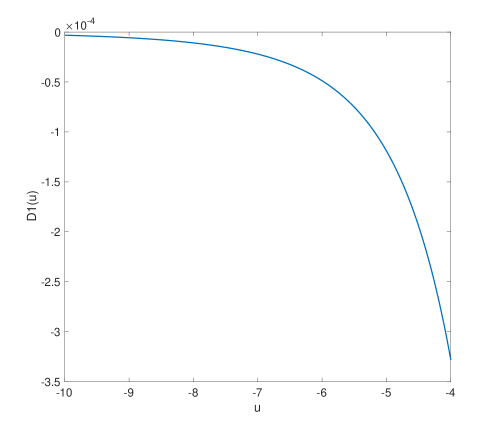
(b) $D_{1}(u)$

Figure 2: The plot of $D_{1}(u)$.

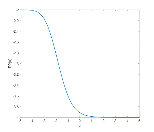
Figure 3: $D_{2}(u)$

Once we have the existence and local uniqueness of the system of equations (3.30) and (3.31) we can follow the substitutions (3.26) and (3.27) to obtain the generalized moment estimators $\widehat{\alpha}_{i,N}$ and $\widehat{\beta}_{i,N}$ for $\alpha_{i}$ and $\beta_{i}$, $i=1,2$. We summarize the above as the following theorem.

Theorem 3.9

Let $(\alpha_{1},\beta_{1},\alpha_{2},\beta_{2})$ be the true parameters such that $(u,v)$ and $(z,\omega)$ defined by (3.26) and (3.27) are in $\mathbb{D}_{1}$ and $\mathbb{D}_{2}$, respectively. Then, when $N$ is sufficiently large the systems of equations (3.30) and (3.31) have solutions $(\widehat{u}_{N},\widehat{v}_{N})$ and $(\widehat{\omega}_{N},\widehat{z}_{N})$, respectively. The solutions are unique in a neighbourhood of $(u,v)$ and a neighbourhood of $(\omega,z)$. If we define

$$\widehat{\alpha}_{1,N} =\frac{(\widehat{u}_{N})^{2}\sigma^{2}}{2(\theta-\widehat{v}_{N})^{2}},\quad\widehat{\alpha}_{2,N}=\frac{(\widehat{\omega}_{N})^{2}\sigma^{2}}{2(\theta-\widehat{z}_{N})^{2}},$$ (3.32)

$$\widehat{\beta}_{1,N} =\widehat{v}_{N}\widehat{\alpha}_{1,N},\quad\widehat{\beta}_{2,N}=\widehat{z}_{N}\widehat{\alpha}_{2,N}\,,$$ (3.33)

then when $N\rightarrow\infty$, we have

$$(\widehat{\alpha}_{1,N}\,,\widehat{\alpha}_{2,N}\,,\widehat{\beta}_{1,N}\,,\widehat{\beta}_{2,N})\rightarrow(\alpha_{1},\alpha_{2},\beta_{1},\beta_{2})\quad\hbox{almost suely}\,.$$

Remark 3.10

If $u=0$, $\omega=0$, i.e., $\frac{\beta_{i}}{\alpha_{i}}=v=z=\theta$, $i=1,2$. We can estimate $(\alpha_{1},\alpha_{2})$ by solving

$$\left\{\begin{aligned} &\frac{\widehat{L}_{1,N}^{\theta}}{\widehat{L}_{0,N}^{\theta}}=-\frac{\sigma}{\sqrt{\pi\alpha_{1}}}+\theta,\\ &\frac{\widehat{R}_{1,N}^{\theta}}{\widehat{R}_{0,N}^{\theta}}=\frac{\sigma}{\sqrt{\pi\alpha_{2}}}+\theta.\\ \end{aligned}\right.$$

Then $\widehat{\beta}_{i}=\theta\widehat{\alpha}_{i}$, $i=1,2$.

We also have the CLT for the above estimators. Before stating the theorem, let us describe the asymptotic variances. Let

$$G_{1}(x)=I(x\leq\theta),\quad G_{2}(x)=xI(x\leq\theta),\quad G_{3}(x)=x^{2}I(x\leq\theta)\,,$$

$$G_{4}(x)=I(x>\theta),\quad G_{5}(x)=xI(x>\theta),\quad G_{6}(x)=x^{2}I(x>\theta)\,.$$

Denote

$$\tilde{\Sigma}_{3}=\left({\sigma}_{ij}\right)_{1\leq i,j\leq 6}\,,\quad\hbox{where}\quad{\sigma}_{ij}=\sigma(G_{i},G_{j})\,,1\leq i,j\leq 6$$

with $\sigma(G_{i},G_{j})$ being defined by (B.40). Then we have as before,

$$\sqrt{N}\left((\widehat{L}_{0,N}^{\theta},\widehat{L}_{1,N}^{\theta},\widehat{L}_{2,N}^{\theta},\widehat{R}_{0,N}^{\theta},\widehat{R}_{1,N}^{\theta},R_{2,N}^{\theta})^{T}-(L_{0}^{\theta},L_{1}^{\theta},L_{2}^{\theta},R_{0}^{\theta},R_{1}^{\theta},R_{2}^{\theta})^{T}\right)\Rightarrow\mathbf{N}(0,\tilde{\Sigma}_{3}).$$

Let $(u,v)=(\kappa_{1}(x_{1},x_{2}),\kappa_{2}(x_{1},x_{2}))$ be the inverse mapping of $(\bar{K}_{1}(u,v),\bar{K}_{2}(u,v))$ defined by (3.30) and let $(\omega,z)=(\kappa_{3}(x_{3},x_{4}),\kappa_{4}(x_{3},x_{4}))$ be the inverse mapping of $(\bar{K}_{3}(u,v),\bar{K}_{4}(u,v))$ defined by (3.31). Comparing with (3.32)-(3.33) and denoting $x=(x_{1},x_{2},x_{3},x_{4},x_{5},x_{6})$, we introduce

$$\rho_{1}(x):=\frac{(\kappa_{1}(\frac{x_{2}}{x_{1}},\frac{x_{3}}{x_{1}}))^{2}\sigma^{2}}{2(\theta-\kappa_{2}(\frac{x_{2}}{x_{1}},\frac{x_{3}}{x_{1}}))^{2}}\,;$$

$$\rho_{2}(x):=\frac{(\kappa_{3}(\frac{x_{5}}{x_{4}},\frac{x_{6}}{x_{4}})^{2}\sigma^{2}}{2(\theta-\kappa_{4}(\frac{x_{5}}{x_{4}},\frac{x_{6}}{x_{4}}))^{2}}\,;$$

$$\rho_{3}(x):=\kappa_{2}(\frac{x_{2}}{x_{1}},\frac{x_{3}}{x_{1}})\rho_{1}(x)\,;$$

$$\rho_{4}(x):=\kappa_{4}(\frac{x_{5}}{x_{4}},\frac{x_{6}}{x_{4}})\rho_{2}(x)\,.$$

Define a map $\rho:\mathbb{R}^{6}\ni x\mapsto(\rho_{1}(x),\rho_{2}(x),\rho_{3}(x),\rho_{4}(x))\in\mathbb{R}^{4}$. Now we establish the following asymptotic normality theorem.

Theorem 3.11

As $N\to\infty$, we have the following asymptotic normality:

$$\sqrt{N}\left((\widehat{\alpha}_{1,N}\,,\widehat{\alpha}_{2,N}\,,\widehat{\beta}_{1,N}\,,\widehat{\beta}_{2,N})^{T}-(\alpha_{1},\alpha_{2},\beta_{1},\beta_{2})^{T}\right)\Rightarrow\mathbf{N}(0,\bar{\Sigma}_{3})\,,$$

where

$$\bar{\Sigma}_{3}=\nabla\rho(L_{0}^{\theta},L_{1}^{\theta},L_{2}^{\theta},R_{0}^{\theta},R_{1}^{\theta},R_{2}^{\theta})\ \tilde{\Sigma}_{3}\nabla\rho(L_{0}^{\theta},L_{1}^{\theta},L_{2}^{\theta},R_{0}^{\theta},R_{1}^{\theta},R_{2}^{\theta})^{T}\,.$$

Theorem 3.9 gives domains $\mathbb{D}_{1}$ and $\mathbb{D}_{2}$ so that we can find generalized moment estimators $\widehat{\alpha}_{1,N}\,,\widehat{\alpha}_{2,N}$ , $\widehat{\beta}_{1,N}\,,\widehat{\beta}_{2,N}$ of $\alpha_{1},\alpha_{2},\beta_{1},\beta_{2}$. On the one hand, although the functions $D_{1}$ and $D_{2}$ are explicit, we still have difficulty to know the shapes of $\mathbb{D}_{1}$ and $\mathbb{D}_{2}$. Our numerical experiments suggest that $D_{1}(u)\not=0$ and $D_{2}(u)\not=0$ for all $u\in\mathbb{R}$. However, we cannot conclude this analytically. On the other hand, as we know that the implicit function theorem is a local one in high dimensions. This means that the solutions to (3.30) and to (3.31) are unique only in a neighbourhood of the true parameters. The method of nondegeneracy of the determinant cannot be used to guarantee the existence of a global inverse function. For example, the mapping $(f(x,y),g(x,y))=(e^{x}\cos y,e^{x}\sin y)$ from $\mathbb{R}^{2}$ to $\mathbb{R}^{2}$ has a strictly positive Jacobian determinant $J(f,g)=e^{x}$ on the whole plane $\mathbb{R}^{2}$. But it is not an injection as a mapping from $\mathbb{R}^{2}$ to $\mathbb{R}^{2}$. Therefore, Theorem 3.9 is powerful when we know a priori roughly the range of the true parameters. For example, in the modelling of the financial market, we know roughly the long memory Hurst parameter $H$ is around $0.5$. But in some other cases researchers do not have any idea about the parameter ranges. Thus, a natural question arises: What should we do if there are more than one solution to (3.30) and to (3.31)? Now we are going to address this global uniqueness issue (existence is not an issue by Theorem 3.9).

From the first equation of (3.30) we have

$$v=\frac{u\frac{\widehat{L}_{1,N}^{\theta}}{\widehat{L}_{0,N}^{\theta}}+\theta A(u)}{u+A(u)}\,.$$ (3.34)

Substituting it to the second equation of (3.30) we obtain

$$u\left(\frac{\widehat{L}_{1,N}^{\theta}}{\widehat{L}_{0,N}^{\theta}}-\theta\right)^{2}+u\left(u\frac{\widehat{L}_{1,N}^{\theta}}{\widehat{L}_{0,N}^{\theta}}+\theta A(u)\right)^{2}$$

$$\qquad\qquad-A(u)\left[\theta^{2}(u+A(u))^{2}-\left(u\frac{\widehat{L}_{1,N}^{\theta}}{\widehat{L}_{0,N}^{\theta}}+\theta A(u)\right)^{2}\right]-u(u+A(u))^{2}\frac{\widehat{L}_{2,N}^{\theta}}{\widehat{L}_{0,N}^{\theta}}=0\,.$$ (3.35)

This is one equation on one unknown $u$. Solving $F_{1}(u)=0$ to get $\widehat{u}_{N}$ and substituting it into (3.34), we can get $\widehat{v}_{N}$. Notice that the quantities $\frac{\widehat{L}_{1,N}^{\theta}}{\widehat{L}_{0,N}^{\theta}}$ and $\frac{\widehat{L}_{2,N}^{\theta}}{\widehat{L}_{0,N}^{\theta}}$ appeared in (3.32) can be computed from real data.

We can proceed similarly for the system of equations (3.31). From its first equation we see

$$z=\frac{\omega\frac{\widehat{R}_{1,N}^{\theta}}{\widehat{R}_{0,N}^{\theta}}-{\theta}B(\omega)}{\omega-B(\omega)}\,.$$ (3.36)

Substituting it to the second equation of (3.31) we have

$$\omega\left(\frac{\widehat{R}_{1,N}^{\theta}}{\widehat{R}_{0,N}^{\theta}}-\theta\right)^{2}+\omega\left(\omega\frac{\widehat{R}_{1,N}^{\theta}}{\widehat{R}_{0,N}^{\theta}}-\theta B(\omega)\right)^{2}$$

$$\qquad\qquad+B(\omega)\left[\theta^{2}(\omega-B(\omega))^{2}-\left(\omega\frac{\widehat{R}_{1,N}^{\theta}}{\widehat{R}_{0,N}^{\theta}}-{\theta}B(\omega)\right)^{2}\right]-\omega(\omega-B(\omega))^{2}\frac{\widehat{R}_{2,N}^{\theta}}{\widehat{R}_{0,N}^{\theta}}=0\,.$$ (3.37)

Denote the left-hand side by $F_{2}(\omega)$. Solving $F_{2}(\omega)=0$ and substituting it into (3.34) yields $\widehat{z}_{N}$. Notice that the quantities $\frac{\widehat{R}_{1,N}^{\theta}}{\widehat{R}_{0,N}^{\theta}}$ and $\frac{\widehat{R}_{2,N}^{\theta}}{\widehat{R}_{0,N}^{\theta}}$ appeared in (3.32) can also be computed from real data. We simulate a sample of the process (1.3) and plot the graphs $F_{1}(u)$ and $F_{2}(\omega)$ in Figure 4. We take $\sigma=1$, $\alpha_{1}=0.1$, $\alpha_{2}=0.5$, $\beta_{1}=0.2$, $\beta_{2}=0.5$, $\theta=0.3$, $h=0.5$, $N=100,000$. It can be seen that since the case of $u=0$ and $\omega=0$ is excluded in Remark 3.10, there exists only one root for $F_{1}$ (or $F_{2}$).

(a) $F_{1}(u)$

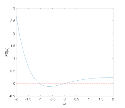
(b) $F_{2}(\omega)$

Figure 4: The plot of $F_{1}(u)$ and $F_{1}(u)$ .

4 Numerical experiments

To validate our estimation scheme discussed in Section 3, we conduct some numerical experiments in this section. Table 1 and Table 2 demonstrate the mean and standard deviation of the estimators $\widehat{\alpha}_{1,n,N}$ and $\widehat{\alpha}_{2,n,N}$ with $\sigma=1$ and taking the order $n\in\{1,2,3,4,5,6,7\}$, $\theta=0$, $\beta_{1}=\beta_{2}=0$ through 1,000 sample paths. Here we set the simulation parameters as: $h=0.5$, $N=100,000$, $X_{0}=0$. Based on the numerical results, it can be seen that the estimators have good consistency and the estimators corresponding the order $n=2,3$ are recommended. By using the built-in function “fsolve” in Matlab to solve the system in (3.21), for given parameters $h=0.5$, $\theta=0.1$, $\beta_{1}=\beta_{2}=0$, and $\sigma=0.6$, we estimate the parameters $\alpha_{1}$ and $\alpha_{2}$ in Table 3 and show the standard deviation in Table 4.

Table 1: Mean of the estimators $\widehat{\alpha}$ through 1,000 sample paths. The true parameters are setting as: $\alpha_{1}=0.02$, $\alpha_{2}=0.05$.

	n
Mean	1	2	3	4	5	6	7
$\alpha_{1}$	0.0198	0.0199	0.0199	0.0200	0.0200	0.0200	0.0201
$\alpha_{2}$	0.0497	0.0497	0.0495	0.0496	0.0497	0.0499	0.0497

Table 2: Standard deviation of the estimators $\widehat{\alpha}$ through 1,000 sample paths. The true parameters are setting as: $\alpha_{1}=0.02$, $\alpha_{2}=0.05$.

	n
Std	1	2	3	4	5	6	7
$\alpha_{1}$	0.0012	0.0011	0.0011	0.0011	0.0012	0.0013	0.0015
$\alpha_{2}$	0.0027	0.0025	0.0023	0.0023	0.0025	0.0026	0.0030

Table 3: Mean of the estimators $\widehat{\alpha}$ through 1,000 sample paths. The true parameters are setting as: $\alpha_{1}=0.1$, $\alpha_{2}=0.2$, $\theta=0.1$

	N($\times 10^{4}$)
Mean	0.8	1.2	1.6	2.0
$\alpha_{1}$	0.0981	0.0979	0.0977	0.0974
$\alpha_{2}$	0.1917	0.1911	0.1910	0.1908

Table 4: Standard deviation of the estimators $\widehat{\alpha}$ through 1,000 sample paths. The true parameters are setting as: $\alpha_{1}=0.1$, $\alpha_{2}=0.2$, $\theta=0.1$

	N($\times 10^{4}$)
Std	0.8	1.2	1.6	2.0
$\alpha_{1}$	0.0094	0.0074	0.0065	0.0056
$\alpha_{2}$	0.0150	0.0122	0.0103	0.0090

5 Conclusion

We conclude the paper here. In this paper, we have proposed the stationary moment estimators for the two-regime threshold OU process. Our approach can be extended to more threshold diffusion processes, including the threshold square-root process, where $X$ is a positive process almost surely with the diffusion term $\sigma(x)=\sum_{i=1}^{m}\sigma_{i}\sqrt{x}I(\theta_{i-1}<x\leq\theta_{i})$, $0=\theta_{0}<\theta_{1}<\theta_{2}<\cdots<\theta_{m}=\infty$. In the multi threshold OU case, the stationary density is given by

$$\psi(x)=\sum_{i=1}^{m}k_{i}\exp\left(\frac{-\alpha_{i}x^{2}+\beta_{i}x}{\sigma_{i}^{2}}\right)I(\theta_{i-1}<x\leq\theta_{i}),$$

with $k_{i}$ determined by $\int_{-\infty}^{\infty}\psi(x)dx$ and $\sigma_{i}^{2}\psi(\theta_{i}-)=\sigma^{2}_{i+1}\psi(\theta_{i}+)$, $i=1,\ldots,m-1$. Notice that $\psi(x)$ may be not continuous at the point $\theta_{i}$. In addition, our estimation approach may be extended to estimate $\alpha_{i}$, $\beta_{i}$, $\theta$, and $\sigma$ simultaneously. For the related reference, we mention the recent work in Cheng et al. (2020). They employed the ergodic theorem for $X_{t_{k}}-X_{t_{k-1}}$, and derived its characteristic function under the stationary distribution. For the threshold process, it is more difficult to conduct these because of the nonlinear term of the threshold process. The problem of estimating $\alpha_{i}$, $\beta_{i}$, $\theta$, and $\sigma$ simultaneously will be studied in a future work.

Appendix A Proof of Proposition 2.4

We compute the transition probability by the spectral expansion method in Linetsky (2005). The proof is similar to Theorem 3.2 in Decamps et al. (2006) and Proposition 3.1 in Wang et al. (2015). So we just show the main computation procedure here. For more details we refer the reader to Proposition 3.1 in Wang et al. (2015). The spectral expansion of the density is written as

$$p_{t}(x,y)=m(y)\sum_{n=1}^{\infty}\exp(-\lambda t)\varphi_{n}(x)\varphi_{n}(y),$$ (A.38)

where $\varphi_{n}(x)$ is the normalized eigenfunction associated to $\lambda_{n}$. It is well-known that

$$\xi(x,\lambda)=\exp\left(z_{1}^{2}/4\right)D_{v}(-z_{1})$$

and

$$\eta(x,\lambda)=\exp\left(z_{2}^{2}/4\right)D_{v}(z_{2})$$

are the solutions with continuous scale derivatives to the following Strum-Liouville equation

$$\frac{1}{2}\sigma^{2}u^{\prime\prime}(x)+(\beta_{1}-\alpha_{1}x)u^{\prime}(x)=-\lambda u(x),\quad x\leq\theta,$$

and

$$\frac{1}{2}\sigma^{2}u^{\prime\prime}(x)+(\beta_{2}-\alpha_{2}x)u^{\prime}(x)=-\lambda u(x),\quad x\geq\theta,$$

respectively.

The Wronskian is given by

$$\omega(\lambda) =\xi(\theta,\lambda)\frac{\eta^{\prime}(\theta,\lambda)}{s(\theta)}-\eta(\theta,\lambda)\frac{\xi^{\prime}(\theta,\lambda)}{s(\theta)},$$

where $\eta^{\prime}(\theta,\lambda)=\frac{\partial\eta(x,\lambda)}{\partial x}\bigg{|}_{x=\theta}$ and $\xi^{\prime}(\theta,\lambda)=\frac{\partial\xi(x,\lambda)}{\partial x}\bigg{|}_{x=\theta}$. Noticing that the Hermite function $H_{v}(z)$ satisfies the recurrence relation (see Lebedev, 1965, Page 289) as

$$\frac{\partial H_{v}(z)}{\partial z}=2vH_{v-1}(z),$$

we get functions $\omega(\lambda)$ and $\varphi_{n}(x)$ in (2.6) and (2.7) respectively. Thus, the proof is completed .

Appendix B Computation of the asymptotic covariances

In this section we compute the covariance $\sigma$ in Theorems 3.5, 3.8 and 3.11 in details by using the invariant measure $\psi_{3}$ given by (3.24) and by the transition probability density function. We give a general formula. For any functions $f$ and $g$ we denote $\langle f\rangle=\int_{\mathbb{R}}f(x)dx$ and $\langle f,g\rangle=\langle fg\rangle$. Let $p_{t}(x,y)$ be the transition density of (1.3) which is also given by (A.38). Define $P_{t}f(x)=\int_{\mathbb{R}}p_{t}(x,y)f(y)dy$. Then, we have $\mathbb{E}\left[g(\widetilde{X}_{kh})|\widetilde{X}_{0}\right]=P_{kh}g(\widetilde{X}_{0})$. For any two functions $f,g:\mathbb{R}\rightarrow\mathbb{R}$ if the following covariance is convergent, then it can be computed as

$$\sigma(f,g) ={\rm Cov}\left[f(\widetilde{X}_{0})\,,g(\widetilde{X}_{0})\right]+\sum_{k=1}^{\infty}{\rm Cov}\left[f(\widetilde{X}_{0})\,,g(\widetilde{X}_{kh})\right]+\sum_{k=1}^{\infty}{\rm Cov}\left[g(\widetilde{X}_{0})\,,f(\widetilde{X}_{kh})\right]$$

$$={\rm Cov}\left[f(\widetilde{X}_{0})\,,g(\widetilde{X}_{0})\right]+\sum_{k=1}^{\infty}\left\{\mathbb{E}\left[f(\widetilde{X}_{0})g(\widetilde{X}_{kh})\right]-\mathbb{E}\left[f(\widetilde{X}_{0})\right]\mathbb{E}\left[g(\widetilde{X}_{kh})\right]\right\}$$

$$\qquad\qquad+\sum_{k=1}^{\infty}\left\{\mathbb{E}\left[g(\widetilde{X}_{0})f(\widetilde{X}_{kh})\right]-\mathbb{E}\left[g(\widetilde{X}_{0})\right]\mathbb{E}\left[f(\widetilde{X}_{kh})\right]\right\}$$

$$={\rm Cov}\left[f(\widetilde{X}_{0})\,,g(\widetilde{X}_{0})\right]+\sum_{k=1}^{\infty}\left\{\mathbb{E}\left[f(\widetilde{X}_{0})(P_{kh}g)(\widetilde{X}_{0})\right]-\mathbb{E}\left[f(\widetilde{X}_{0})\right]\mathbb{E}\left[(P_{kh}g)(\widetilde{X}_{0})\right]\right\}$$

$$\qquad\qquad+\sum_{k=1}^{\infty}\left\{\mathbb{E}\left[g(\widetilde{X}_{0})(P_{kh}f)(\widetilde{X}_{0})\right]-\mathbb{E}\left[g(\widetilde{X}_{0})\right]\mathbb{E}\left[(P_{kh}f)(\widetilde{X}_{0})\right]\right\}\,.$$

Denote $\psi_{f}:=\sum_{k=1}^{\infty}P_{kh}f$ and $\widehat{\psi}_{f}=\psi_{f}-\langle\psi_{3},\psi_{f}\rangle$. Then, we have

$$\psi_{f}=(I-P_{h})^{-1}P_{h}f\,,\quad\widehat{\psi}_{f}=(I-P_{h})^{-1}P_{h}f-\langle\psi_{3},(I-P_{h})^{-1}P_{h}f\rangle\,.$$ (B.39)

We also denote $\widehat{f}=f-\langle\psi_{3},f\rangle=\langle\psi_{3}f\rangle$. With these notations, we have

$${\sigma}(f,g) =\langle\psi_{3}fg\rangle-\langle\psi_{3}f\rangle\langle\psi_{3}g\rangle+\langle\psi_{3}g\psi_{f}\rangle-\langle\psi_{3}g\rangle\langle\psi_{3}\psi_{f}\rangle+\langle\psi_{3}f\psi_{g}\rangle-\langle\psi_{3}f\rangle\langle\psi_{3}\psi_{g}\rangle$$

$$=\langle\psi_{3}\widehat{f}\widehat{g}\rangle+\langle\psi_{3}g\widehat{\psi}_{f}\rangle+\langle\psi_{3}f\widehat{\psi}_{g}\rangle\,.$$ (B.40)

Declarations of interest: none.

References

- Bass and Pardoux (1987) R. F. Bass and É. Pardoux. Uniqueness for diffusions with piecewise constant coefficients. Probab. Theory Related Fields, 76(4):557–572, 1987. ISSN 0178-8051. doi: 10.1007/BF00960074. URL https://doi.org/10.1007/BF00960074.
- Brockwell et al. (1991) Peter J. Brockwell, Rob J. Hyndman, and Gary K. Grunwald. Continuous time threshold autoregressive models. Statist. Sinica, 1(2):401–410, 1991. ISSN 1017-0405.
- Brockwell et al. (2007) Peter J. Brockwell, Richard A. Davis, and Yu Yang. Continuous-time Gaussian autoregression. Statistica Sinica, 17(1):63–80, 2007. ISSN 10170405, 19968507. URL http://www.jstor.org/stable/26432511.
- Brockwell and Hyndman (1992) P.J. Brockwell and R.J. Hyndman. On continuous-time threshold autoregression. International Journal of Forecasting, 8(2):157 – 173, 1992. ISSN 0169-2070. doi: https://doi.org/10.1016/0169-2070(92)90116-Q. URL http://www.sciencedirect.com/science/article/pii/016920709290116Q.
- Brooks et al. (2011) Steve Brooks, Andrew Gelman, Galin L. Jones, and Xiao-Li Meng, editors. Handbook of Markov chain Monte Carlo. Chapman & Hall/CRC Handbooks of Modern Statistical Methods. CRC Press, Boca Raton, FL, 2011. ISBN 978-1-4200-7941-8. doi: 10.1201/b10905. URL https://doi.org/10.1201/b10905.
- Browne and Whitt (1995) Sid Browne and Ward Whitt. Piecewise-linear diffusion processes. In Advances in queueing, Probab. Stochastics Ser., pages 463–480. CRC, Boca Raton, FL, 1995.
- Buchholz (1969) Herbert Buchholz. The confluent hypergeometric function with special emphasis on its applications. Translated from the German by H. Lichtblau and K. Wetzel. Springer Tracts in Natural Philosophy, Vol. 15. Springer-Verlag New York Inc., New York, 1969.
- Chan (1993) K. S. Chan. Consistency and limiting distribution of the least squares estimator of a threshold autoregressive model. Ann. Statist., 21(1):520–533, 1993. ISSN 0090-5364. doi: 10.1214/aos/1176349040. URL https://doi.org/10.1214/aos/1176349040.
- Cheng et al. (2020) Yiying Cheng, Yaozhong Hu, and Hongwei Long. Generalized moment estimators for -stable Ornstein-Uhlenbeck motions from discrete observations. Stat. Inference Stoch. Process., 23(1):53–81, 2020. ISSN 1387-0874. doi: 10.1007/s11203-019-09201-4. URL https://doi.org/10.1007/s11203-019-09201-4.
- Chi et al. (2017) Zeyu Chi, Fangyuan Dong, and Hoi Ying Wong. Option pricing with threshold mean reversion. Journal of Futures Markets, 37(2):107–131, 2017. doi: 10.1002/fut.21795. URL https://onlinelibrary.wiley.com/doi/abs/10.1002/fut.21795.
- Decamps et al. (2006) Marc Decamps, Marc Goovaerts, and Wim Schoutens. Self exciting threshold interest rates models. Int. J. Theor. Appl. Finance, 9(7):1093–1122, 2006. ISSN 0219-0249. doi: 10.1142/S0219024906003937. URL https://doi.org/10.1142/S0219024906003937.
- Ding et al. (2020) Kailin Ding, Zhenyu Cui, and Yongjin Wang. A markov chain approximation scheme for option pricing under skew diffusions. Quantitative Finance, 0(0):1–20, 2020. doi: 10.1080/14697688.2020.1781235. URL https://doi.org/10.1080/14697688.2020.1781235.
- Gairat and Shcherbakov (2017) Alexander Gairat and Vadim Shcherbakov. Density of skew Brownian motion and its functionals with application in finance. Math. Finance, 27(4):1069–1088, 2017. ISSN 0960-1627. doi: 10.1111/mafi.12120. URL https://doi.org/10.1111/mafi.12120.
- Hu and Song (2013) Yaozhong Hu and Jian Song. Parameter estimation for fractional Ornstein-Uhlenbeck processes with discrete observations. In Malliavin calculus and stochastic analysis, volume 34 of Springer Proc. Math. Stat., pages 427–442. Springer, New York, 2013. doi: 10.1007/978-1-4614-5906-4˙19. URL https://doi.org/10.1007/978-1-4614-5906-4_19.
- Hu et al. (2015) Yaozhong Hu, Chihoon Lee, Myung Hee Lee, and Jian Song. Parameter estimation for reflected Ornstein-Uhlenbeck processes with discrete observations. Stat. Inference Stoch. Process., 18(3):279–291, 2015. ISSN 1387-0874. doi: 10.1007/s11203-014-9112-7. URL https://doi.org/10.1007/s11203-014-9112-7.
- Jiang et al. (2018) Yiming Jiang, Shiyu Song, and Yongjin Wang. Pricing European vanilla options under a jump-to-default threshold diffusion model. J. Comput. Appl. Math., 344:438–456, 2018. ISSN 0377-0427. doi: 10.1016/j.cam.2018.04.039. URL https://doi.org/10.1016/j.cam.2018.04.039.
- Karlin and Taylor (1981) Samuel Karlin and Howard M. Taylor. A second course in stochastic processes. Academic Press, Inc. [Harcourt Brace Jovanovich, Publishers], New York-London, 1981.
- Kutoyants (2012) Yury A. Kutoyants. On identification of the threshold diffusion processes. Ann. Inst. Statist. Math., 64(2):383–413, 2012. ISSN 0020-3157. doi: 10.1007/s10463-010-0318-1. URL https://doi.org/10.1007/s10463-010-0318-1.
- Lebedev (1965) N. N. Lebedev. Special functions and their applications. Revised English edition. Translated and edited by Richard A. Silverman. Prentice-Hall, Inc., Englewood Cliffs, N.J., 1965.
- Lejay and Pigato (2020) Antoine Lejay and Paolo Pigato. Maximum likelihood drift estimation for a threshold diffusion. Scandinavian Journal of Statistics, 47(3):609–637, 2020. doi: 10.1111/sjos.12417. URL https://onlinelibrary.wiley.com/doi/abs/10.1111/sjos.12417.
- Linetsky (2005) Vadim Linetsky. On the transition densities for reflected diffusions. Adv. in Appl. Probab., 37(2):435–460, 2005. ISSN 0001-8678. doi: 10.1239/aap/1118858633. URL https://doi.org/10.1239/aap/1118858633.
- Meyn and Tweedie (2009) Sean Meyn and Richard L. Tweedie. Markov chains and stochastic stability. Cambridge University Press, Cambridge, second edition, 2009. ISBN 978-0-521-73182-9. doi: 10.1017/CBO9780511626630. URL https://doi.org/10.1017/CBO9780511626630. With a prologue by Peter W. Glynn.
- Meyn and Tweedie (1993) Sean P. Meyn and R. L. Tweedie. Stability of Markovian processes. II. Continuous-time processes and sampled chains. Adv. in Appl. Probab., 25(3):487–517, 1993. ISSN 0001-8678. doi: 10.2307/1427521. URL https://doi.org/10.2307/1427521.
- Siu (2016) Tak Kuen Siu. A self-exciting threshold jump-diffusion model for option valuation. Insurance Math. Econom., 69:168–193, 2016. ISSN 0167-6687. doi: 10.1016/j.insmatheco.2016.05.008. URL https://doi.org/10.1016/j.insmatheco.2016.05.008.
- Siu et al. (2006) Tak Kuen Siu, Howell Tong, and Hailiang Yang. Option pricing under threshold autoregressive models by threshold Esscher transform. J. Ind. Manag. Optim., 2(2):177–197, 2006. ISSN 1547-5816. doi: 10.3934/jimo.2006.2.177. URL https://doi.org/10.3934/jimo.2006.2.177.
- Stramer and Roberts (2007) O. Stramer and G. O. Roberts. On Bayesian analysis of nonlinear continuous-time autoregression models. J. Time Ser. Anal., 28(5):744–762, 2007. ISSN 0143-9782. doi: 10.1111/j.1467-9892.2007.00549.x. URL https://doi.org/10.1111/j.1467-9892.2007.00549.x.
- Stramer et al. (1996) O. Stramer, R. L. Tweedie, and P. J. Brockwell. Existence and stability of continuous time threshold ARMA processes. Statist. Sinica, 6(3):715–732, 1996. ISSN 1017-0405.
- Su and Chan (2015) Fei Su and Kung-Sik Chan. Quasi-likelihood estimation of a threshold diffusion process. J. Econometrics, 189(2):473–484, 2015. ISSN 0304-4076. doi: 10.1016/j.jeconom.2015.03.038. URL https://doi.org/10.1016/j.jeconom.2015.03.038.
- Su and Chan (2017) Fei Su and Kung-Sik Chan. Testing for threshold diffusion. J. Bus. Econom. Statist., 35(2):218–227, 2017. ISSN 0735-0015. doi: 10.1080/07350015.2015.1073594. URL https://doi.org/10.1080/07350015.2015.1073594.
- Tong (1983) Howell Tong. Threshold models in nonlinear time series analysis, volume 21 of Lecture Notes in Statistics. Springer-Verlag, New York, 1983. ISBN 0-387-90918-4. doi: 10.1007/978-1-4684-7888-4. URL https://doi.org/10.1007/978-1-4684-7888-4.
- van der Vaart (1998) A. W. van der Vaart. Asymptotic statistics, volume 3 of Cambridge Series in Statistical and Probabilistic Mathematics. Cambridge University Press, Cambridge, 1998. ISBN 0-521-49603-9; 0-521-78450-6. doi: 10.1017/CBO9780511802256. URL https://doi.org/10.1017/CBO9780511802256.
- Wang et al. (2015) Suxin Wang, Shiyu Song, and Yongjin Wang. Skew Ornstein-Uhlenbeck processes and their financial applications. J. Comput. Appl. Math., 273:363–382, 2015. ISSN 0377-0427. doi: 10.1016/j.cam.2014.06.023. URL https://doi.org/10.1016/j.cam.2014.06.023.
- Zhuo and Menoukeu-Pamen (2017) Xiaoyang Zhuo and Olivier Menoukeu-Pamen. Efficient piecewise trees for the generalized skew Vasicek model with discontinuous drift. Int. J. Theor. Appl. Finance, 20(4):1750028, 34, 2017. ISSN 0219-0249. doi: 10.1142/S0219024917500285. URL https://doi.org/10.1142/S0219024917500285.
- Zhuo et al. (2017) Xiaoyang Zhuo, Guangli Xu, and Haoyan Zhang. A simple trinomial lattice approach for the skew-extended CIR models. Math. Financ. Econ., 11(4):499–526, 2017. ISSN 1862-9679. doi: 10.1007/s11579-017-0192-1. URL https://doi.org/10.1007/s11579-017-0192-1.