Delayed finite-dimensional observer-based control of 1D parabolic PDEs via reduced-order LMIs

Abstract

Recently a constructive method was introduced for finite-dimensional observer-based control of 1D parabolic PDEs. In this paper we present an improved method in terms of the reduced-order LMIs (that significantly shorten the computation time) and introduce predictors to manage with larger delays. We treat the case of a 1D heat equation under Neumann actuation and non-local measurement, that has not been studied yet. We apply modal decomposition and prove $L^{2}$ exponential stability by a direct Lyapunov method. We provide reduced-order LMI conditions for finding the observer dimension $N$ and resulting decay rate. The LMI dimension does not grow with $N$. The LMI is always feasible for large $N$, and feasibility for $N$ implies feasibility for $N+1$. For the first time we manage with delayed implementation of the controller in the presence of fast-varying (without any constraints on the delay-derivative) input and output delays. To manage with larger delays, we construct classical observer-based predictors. For the known input delay, the LMIs dimension does not grow with $N$, whereas for unknown one the LMIs dimension grows, but it is essentially smaller than in the existing results. A numerical example demonstrates the efficiency of our method.

1 Introduction

Observer-based controllers for PDEs with observers in the form of PDEs have been constructed in [4, 22, 21] (to name a few). Very attractive for practical applications finite-dimensional observer-based controllers for parabolic systems was studied by using the modal decomposition approach in [2, 3, 4, 9, 10]. The recent papers [15, 16, 18] on constructive LMI-based finite-dimensional observer-based control have introduced $N$-dimensional observers, where the gains (as well as the controller gains) are based only on the $N_{0}\leq N$ unstable modes. However, the stability analysis was based on the full-order closed-loop systems. The latter led to higher-order LMIs whose dimension grows with $N$ and complicated proofs of their feasibility.

Delayed and/or sampled-data finite-dimensional controllers were designed in [8, 11, 29] for distributed static output-feedback control and in [13, 6] for boundary state-feedback control. Delayed implementation of finite-dimensional observer-based controllers for the 1D heat equation was presented in [17]. In the case of Dirichlet actuation considered in [17], the results were not applicable to the case where both input and output delays are fast-varying (without any constraints on the time-derivative that correspond e.g. to sampled-data and network-based control). For boundary control in the presence of fast-varying input and output delays only infinite-dimensional PDE observers have been suggested till now [19].

Large input delays for PDEs can be compensated by classical predictors [20]. Predictor-based controllers for ODEs that compensated an arbitrary large constant part of a delay were suggested in [12, 25, 28] and extended to state-feedback boundary control of parabolic PDEs in [23, 27]. For coupled systems of ODEs, predictors may enlarge the constant part of the delay which preserves stability, but cannot manage with arbitrary large constant delays due to coupling [24, 30]. However, the finite-dimensional observer-based predictors have not been constructed yet for PDEs.

In the present paper, we introduce finite-dimensional observer-based controllers for the 1D heat equation under Neumann actuation and non-local measurement. We apply modal decomposition to the original system (without dynamic extension) and prove $L^{2}$ exponential stability of the closed-loop system by a direct Lyapunov method. The paper contribution to challenging finite-dimensional observer-based control can be summarized as follows:

1. The paper introduces reduced-order closed-loop system that reveals the singularly perturbed structure of the system, leads to reduced-order LMIs, trivializes the LMIs feasibility proof and the fact that their feasibility for the observer dimension $N$ implies feasibility for $N+1$. In example, the feasibility of the reduced-order LMIs for the delayed case can be easily verified for $N=30$, whereas in [17] the corresponding conditions could not be verified for $N=9$. Note that larger $N$ enlargers delays that preserve the stability.

2. For the first time in the case of boundary control, the results are applicable to fast-varying input and output delays. This is because the proportional controller under Neumann actuation and non-local measurement leads to $L^{2}$ convergence. For briefness, our results are presented for differentiable delays. However, via the time-delay approach to networked control [7], the same LMI conditions are applicable to networked control implementation via a zero-order-hold device, under sampled-data delayed measurements.

3. The first finite-dimensional observer-based predictor is constructed to compensate the constant part of input fast-varying delay, and this is in the presence of the small output fast-varying delay. We present the classical predictors using the reduction approach [1]. We predict the future state of the observer, whereas the infinite-dimensional part depends on the uncompensated large delay. We consider the case of either known or unknown input delay. For the known input delay, the LMIs dimension does not grow with $N$, whereas for the unknown one it grows, but is essentially smaller than in [17]. An example demonstrates the efficiency of the method and shows that predictors allow for larger delays which preserve the stability.

Our new method can be applied to other classes of parabolic PDEs (see Remark 2.1 below). In the conference version of the paper [14] predictors were not considered.

Notations and preliminaries: $L^{2}(0,1)$ is the Hilbert space of Lebesgue measurable and square integrable functions $f:[0,1]\to\mathbb{R}$ with inner product $\left<f,g\right>:=\scriptsize{\int_{0}^{1}f(x)g(x)dx}$ and norm $\left\|f\right\|^{2}:=\left<f,f\right>$. $H^{k}(0,1)$ is the Sobolev space of functions $f:[0,1]\to\mathbb{R}$ having $k$ square integrable weak derivative, with norm $\left\|f\right\|^{2}_{H^{k}}:={\color[rgb]{0,0,1}\sum_{j=0}^{k}\left\|\frac{\text{d}^{j}f}{\text{dx}^{j}}\right\|^{2}}$. The Euclidean norm on $\mathbb{R}^{n}$ will be denoted by $\left|\cdot\right|$. For $P\in\mathbb{R}^{n\times n}$, the notation $P>0$ means that $P$ is symmetric and positive definite. The sub-diagonal elements of a symmetric matrix are denoted by $*.$ For $U\in\mathbb{R}^{n\times n},\ U>0$ and $X\in\mathbb{R}^{n}$ we denote $\left|X\right|^{2}_{U}=X^{T}UX$. We denote by $\mathbb{Z}_{+}$ the set of nonnegative integers.

Recall that the Sturm-Liouville eigenvalue problem

$$\begin{array}[]{lll}&\phi^{\prime\prime}+\lambda\phi=0,\ \ x\in[0,1]\quad;\quad\phi^{\prime}(0)=\phi^{\prime}(1)=0,\end{array}$$ (1.1)

induces a sequence of eigenvalues $\scriptsize\lambda_{n}=n^{2}\pi^{2},n\geq 0$ with corresponding eigenfunctions

$$\begin{array}[]{lll}\phi_{0}(x)=1,\quad\phi_{n}(x)=\sqrt{2}\cos\left(\sqrt{\lambda_{n}}x\right),n\geq 1.\end{array}$$ (1.2)

Moreover, the eigenfunctions form a complete orthonormal system in $L^{2}(0,1)$. Given $N\in\mathbb{Z}_{+}$ and $h\in L^{2}(0,1)$ satisfying $h\overset{L^{2}}{=}\sum_{n=0}^{\infty}h_{n}\phi_{n}$ we will use the notation $\left\|h\right\|_{N}^{2}=\left\|h\right\|^{2}-\sum_{n=0}^{N}h_{n}^{2}=\sum_{n=N+1}^{\infty}h_{n}^{2}$.

2 Non-delayed $L^{2}$-stabilization

Consider the reaction-diffusion system

$$z_{t}(x,t)=z_{xx}(x,t)+qz(x,t),\ z_{x}(0,t)=0,\ z_{x}(1,t)=u(t)$$ (2.1)

where $t\geq 0$, $x\in[0,1]$, $z(x,t)\in\mathbb{R}$ and $q\in\mathbb{R}$ is the reaction coefficient. We consider Neumann actuation with a control input $u(t)$ and non-local measurement of the form

$$y(t)=\left<c,z(\cdot,t)\right>,\quad c\in L^{2}(0,1).$$ (2.2)

Below, we prove the existence and uniqueness of a classical solution to (2.1) (see proof after (2.14)). Therefore, we can present the solution as

$$z(x,t)\overset{L^{2}}{=}\sum_{n=0}^{\infty}z_{n}(t)\phi_{n}(x),\ \ z_{n}(t)=\left<z(\cdot,t),\phi_{n}\right>.$$ (2.3)

with $\phi_{n}(t),\ n\in\mathbb{Z}_{+}$ given in (1.2) (see e.g [3, 13]). Differentiating $z_{n}(t)$ and substituting $z_{t}=z_{xx}+qz$ we have

$$\begin{array}[]{lll}\dot{z}_{n}(t)\!=\!\int_{0}^{1}z_{t}(x,t)\phi_{n}(x)dx\!=\int_{0}^{1}z_{xx}(x,t)\phi_{n}(x)dx+qz_{n}(t).\end{array}$$

Integrating by parts twice and using the boundary conditions for $z$ and $\phi_{n}$ we find

$$\begin{array}[]{lll}&\int_{0}^{1}z_{xx}(x,t)\phi_{n}(x)dx=-\lambda_{n}z_{n}(t)+\phi_{n}(1)u(t)\end{array}$$

which leads to

$$\dot{z}_{n}(t)=(-\lambda_{n}+q)z_{n}(t)+b_{n}u(t),\quad t\geq 0,$$ (2.4)

$$b_{0}=1,\ \ b_{n}={(-1)}^{n}\sqrt{2},\ n\in\mathbb{Z}_{+}.$$

In particular, note that

$$b_{n}\neq 0,\quad n\in\mathbb{Z}_{+}$$ (2.5)

and for $N\geq 0$ the following holds:

$$\begin{array}[]{lll}&\sum_{n=N+1}^{\infty}b_{n}^{2}\lambda_{n}^{-1}=\frac{2}{\pi^{2}}\sum_{n=N+1}^{\infty}\frac{1}{n^{2}}\leq\frac{2}{\pi^{2}N}.\end{array}$$ (2.6)

Let $\delta>0$ be a desired decay rate. Since $\lim_{n\to\infty}\lambda_{n}=\infty$, there exists some $N_{0}\in\mathbb{Z}_{+}$ such that

$$-\lambda_{n}+q<-\delta,\quad n>N_{0}.$$ (2.7)

Let $N\geq N_{0}+1$, where $N$ will define the dimension of the observer, whereas $N_{0}$ will be the dimension of the controller. We construct a $N$-dimensional observer of the form

$$\hat{z}(x,t):=\sum_{n=0}^{N}\hat{z}_{n}(t)\phi_{n}(x)$$ (2.8)

where $\hat{z}_{n}(t)$ satisfy the ODEs for $t\geq 0$

$$\begin{array}[]{lll}\dot{\hat{z}}_{n}(t)&=(-\lambda_{n}+q)\hat{z}_{n}(t)+b_{n}u(t)\\ &-l_{n}\left[\left<\sum_{n=0}^{N}\hat{z}_{n}(t)\phi_{n},c\right>-y(t)\right],\\ \hat{z}_{n}(0)&=0,\quad 0\leq n\leq N.\end{array}$$ (2.9)

Here $l_{n},\ 0\leq n\leq N$ are scalars, and $l_{N_{0}+1}=...=l_{N}=0$. We further choose $l_{N_{0}+1}=...=l_{N}=0$. This choice will lead to a reduced-order closed-loop system (see (2.25), (2.26) below) with omitted ODEs for $\hat{z}_{N_{0}+1},...,\hat{z}_{N}$ and will not deteriorate the performance of the closed-loop system. Let

$$\begin{array}[]{ll}&A_{0}=\operatorname{diag}\left\{-\lambda_{i}+q\right\}_{i=0}^{N_{0}},\ L_{0}=\operatorname{col}\left\{l_{i}\right\}_{i=0}^{N_{0}}\\ &B_{0}=\operatorname{col}\left\{b_{i}\right\}_{i=0}^{N_{0}},\ C_{0}=\left[c_{0},\dots,c_{N_{0}}\right],\ c_{n}=\left<c,\phi_{n}\right>.\end{array}$$ (2.10)

Assume that

$$c_{n}\neq 0,\quad 0\leq n\leq N_{0}.$$ (2.11)

By the Hautus lemma $(A_{0},C_{0})$ is observable. We choose $L_{0}=[l_{0},\dots,l_{N_{0}}]^{T}$ which satisfies the Lyapunov inequality:

$$P_{\text{o}}(A_{0}-L_{0}C_{0})+(A_{0}-L_{0}C_{0})^{T}P_{\text{o}}<-2\delta P_{\text{o}}$$ (2.12)

with $0<P_{\text{o}}\in\mathbb{R}^{(N_{0}+1)\times(N_{0}+1)}$. By the Hautus lemma, $(A_{0},B_{0})$ is controllable due to (2.5). Let $K_{0}\in\mathbb{R}^{1\times(N_{0}+1)}$ satisfy the Lyapunov inequality

$$\begin{array}[]{lll}&P_{\text{c}}(A_{0}+B_{0}K_{0})+(A_{0}+B_{0}K_{0})^{T}P_{\text{c}}<-2\delta P_{\text{c}},\end{array}$$ (2.13)

where $0<P_{\text{c}}\in\mathbb{R}^{(N_{0}+1)\times(N_{0}+1)}$. We propose a controller

$$u(t)=K_{0}\hat{z}^{N_{0}}(t),\quad\hat{z}^{N_{0}}(t)=\left[\hat{z}_{0}(t),\dots,\hat{z}_{N_{0}}(t)\right]^{T}$$ (2.14)

which is based on the $N$-dimensional observer (2.9). Note that (2.9) implies $u(0)=0$.

For well-posedness we introduce the change of variables $w(x,t)=z(x,t)-\frac{1}{2}x^{2}u(t)$ leading to the equivalent PDE

$$\begin{array}[]{lll}&w_{t}(x,t)=w_{xx}(x,t)+qw(x,t)+f(x,t),\ x\in[0,1],\ t\geq 0,\\ &f(x,t)=-\frac{1}{2}x^{2}\dot{u}(t)+\left(\frac{q}{2}x^{2}+1\right)u(t),\\ &w_{x}(0,t)=0,\quad w_{x}(1,t)=0.\end{array}$$ (2.15)

Consider the operator

$$\begin{array}[]{lll}&{\color[rgb]{0,0,1}\mathfrak{A}}:\mathcal{D}({\color[rgb]{0,0,1}\mathfrak{A}})\subseteq L^{2}(0,1)\to L^{2}(0,1),\ \ {\color[rgb]{0,0,1}\mathfrak{A}}h=-h^{\prime\prime},\\ &\mathcal{D}({\color[rgb]{0,0,1}\mathfrak{A}})=\left\{h\in H^{2}(0,1)|h^{\prime}(0)=h^{\prime}(1)=0\right\}.\end{array}$$ (2.16)

It is well known that ${\color[rgb]{0,0,1}\mathfrak{A}}$ generates a strongly continuous semigroup on $L^{2}(0,1)$ [26]. Let ${\color[rgb]{0,0,1}\mathbb{G}}=L^{2}(0,1)\times\mathbb{R}^{N+1}$ be a Hilbert space with the norm $\left\|\cdot\right\|_{{\color[rgb]{0,0,1}\mathbb{G}}}=\sqrt{\left\|\cdot\right\|+\left|\cdot\right|}$. Defining the state $\xi(t)=\text{col}\left\{w(\cdot,t),\hat{z}^{N}(t)\right\}$, where

$$\begin{array}[]{lll}\hat{z}^{N}(t)=\text{col}\left\{\hat{z}_{0}(t),\dots,\hat{z}_{N}(t)\right\}\end{array}$$ (2.17)

the closed-loop system (2.9), (2.14) and (2.15) can be presented as

$$\frac{\text{d}}{\text{dt}}\xi(t)+\operatorname{diag}\left\{{\color[rgb]{0,0,1}\mathfrak{A}},{\color[rgb]{0,0,1}\mathfrak{B}}\right\}\xi(t)=\operatorname{col}\left\{f_{1}(\xi),f_{2}(\xi)\right\}$$

where

$$\begin{array}[]{lll}&{\color[rgb]{0,0,1}\mathfrak{B}}\xi_{2}\scriptsize=\begin{bmatrix}-\left(A_{0}+B_{0}K_{0}-L_{0}C_{0}\right)&L_{0}C_{1}\\ -B_{1}K_{0}&-A_{1}\end{bmatrix}\xi_{2},\ \ \xi_{2}\in\mathbb{R}^{N+1},\\ &f_{1}(\xi)=\scriptsize\begin{bmatrix}q&\upsilon&\frac{x^{2}}{2}K_{0}L_{0}C_{1}\end{bmatrix}\normalsize\xi-\frac{x^{2}}{2}K_{0}L_{0}\left<c,\xi_{1}\right>,\\ &f_{2}(\xi)=\text{col}\left\{L_{0}\left<c,\xi_{1}\right>+\frac{1}{2}\left<c,x^{2}\right>K_{0}\xi_{2},0\right\},\\ &\upsilon=\left(\frac{q}{2}x^{2}+1\right)K_{0}-\frac{x^{2}}{2}K_{0}(A_{0}+B_{0}K_{0}-L_{0}C_{0})\\ &\hskip 14.22636pt+\frac{1}{2}\left<c,x^{2}\right>L_{0}K_{0}.\end{array}$$

$f_{1}$ and $f_{2}$ are linear and, therefore, continuously differentiable. Let $z(\cdot,0)=w(\cdot,0)\in H^{1}(0,1)$. By Theorems 6.3.1 and 6.3.3 in [26], there exists a unique classical solution

$$\xi\in C\left([0,\infty);{\color[rgb]{0,0,1}\mathbb{G}}\right)\cap C^{1}\left((0,\infty);{\color[rgb]{0,0,1}\mathbb{G}}\right)$$ (2.18)

satisfying $\xi(t)\in\mathcal{D}\left({\color[rgb]{0,0,1}\mathfrak{A}}\right)\times\mathbb{R}^{N+1},\ t>0$. Applying $z(x,t)=w(x,t)+\frac{1}{2}x^{2}u(t)$, (2.1) and (2.9), subject to (2.14), have a unique classical solution such that $z\in C([0,\infty),L^{2}(0,1))\cap C^{1}((0,\infty),L^{2}(0,1))$ and $z(\cdot,t)\in H^{2}(0,1)$ with $z_{x}(0,t)=0,\ z_{x}(1,t)=u(t)$ for $t\in[0,\infty)$.

Let

$$e_{n}(t)=z_{n}(t)-\hat{z}_{n}(t),\ 0\leq n\leq N$$ (2.19)

be the estimation error. The last term on the right-hand side of (2.9) can be written as

$$\begin{array}[]{ll}&\int_{0}^{1}c(x)\left[\sum_{n=1}^{N}\hat{z}_{n}(t)\phi_{n}(x)-\sum_{n=1}^{\infty}z_{n}(t)\phi_{n}(x)\right]dx\\ &=-\sum_{n=0}^{N}c_{n}e_{n}(t)-\zeta(t),\ \zeta(t)=\sum_{n=N+1}^{\infty}c_{n}z_{n}(t).\end{array}$$ (2.20)

Then the error equations for $0\leq n\leq N$ and $t\geq 0$ are

$$\begin{array}[]{r}\dot{e}_{n}(t)=(-\lambda_{n}+q)e_{n}(t)-l_{n}\left(\sum_{n=1}^{N}c_{n}e_{n}(t)+\zeta(t)\right).\end{array}$$ (2.21)

Using the Young inequality, we obtain the bound

$$\begin{array}[]{lll}\zeta^{2}(t)&\leq\left\|c\right\|_{N}^{2}\sum_{n=N+1}^{\infty}z_{n}^{2}(t).\end{array}$$ (2.22)

Denote

$$\begin{array}[]{lllllll}&e^{N_{0}}(t)=\operatorname{col}\left\{e_{n}(t)\right\}_{n=1}^{N_{0}},\ e^{N-N_{0}}(t)=\operatorname{col}\left\{e_{n}(t)\right\}_{n=N_{0}+1}^{N},\\ &\hat{z}^{N-N_{0}}(t)=\operatorname{col}\left\{\hat{z}_{n}(t)\right\}_{n=N_{0}+1}^{N},\ \mathcal{L}_{0}=\text{col}\left\{L_{0},-L_{0}\right\},\\ &\mathcal{K}_{0}=\begin{bmatrix}K_{0},&0_{1\times(N_{0}+1)}\end{bmatrix},\ A_{1}=\operatorname{diag}\left\{-\lambda_{i}+q\right\}_{i=N_{0}+1}^{N},\\ &B_{1}=\left[b_{N_{0}+1},\dots,b_{N}\right]^{T},\ C_{1}=\left[c_{N_{0}+1},\dots,c_{N}\right],\end{array}$$ (2.23)

and

$$\begin{array}[]{lllllll}&F_{0}=\scriptsize\begin{bmatrix}A_{0}+B_{0}K_{0}&L_{0}C_{0}\\ 0&A_{0}-L_{0}C_{0}\end{bmatrix},\ X_{0}(t)=\scriptsize\begin{bmatrix}\hat{z}^{N_{0}}(t)\\ e^{N_{0}}(t)\end{bmatrix}.\end{array}$$ (2.24)

From (2.3), (2.9), (2.10), (2.14), (2.21), (2.23) and (2.24) we observe that $e^{N-N_{0}}(t)$ satisfies

$$\dot{e}^{N-N_{0}}(t)=A_{1}e^{N-N_{0}}(t)$$ (2.25)

and is exponentially decaying, whereas the reduced-order closed-loop system

$$\dot{X}_{0}(t)=F_{0}X_{0}(t)+\mathcal{L}_{0}C_{1}e^{N-N_{0}}(t)+\mathcal{L}_{0}\zeta(t),$$ (2.26)

$$\dot{z}_{n}(t)=(-\lambda_{n}+q)z_{n}(t)+b_{n}\mathcal{K}_{0}X_{0}(t),\ n>N.$$

with $\zeta(t)$ subject to (2.22) does not depend on $\hat{z}^{N-N_{0}}(t)$. Moreover, $\hat{z}^{N-N_{0}}(t)$ satisfies

$$\dot{\hat{z}}^{N-N_{0}}(t)=A_{1}\hat{z}^{N-N_{0}}(t)+B_{1}\mathcal{K}_{0}X_{0}(t)$$ (2.27)

and is exponentially decaying provided $X_{0}(t)$ is exponentially decaying. Therefore, for stability of (2.1) under the control law (2.14) it is sufficient to show stability of the reduced-order system (2.26). The latter can be considered as a singularly perturbed system with the slow state $X_{0}(t)$ and the fast infinite-dimensional state $z_{n}(t),\ n>N$.

Note that in [15], the full-order closed-loop system with the states $X_{0},\hat{z}^{N-N_{0}},e^{N-N_{0}},z_{n}\ \ (n>N)$ was considered, leading to full-order LMI conditions for stability. In the present paper we derive stability conditions for the reduced-order system (2.26) in terms of reduced-order LMI (see (2.29) below) for finding $N$ and the exponential decay rate $\delta$. Differently from [15], the dimension of this LMI will not grow with $N$. Its feasibility for large $N$ will follow directly from the application of Schur complements. Moreover, if this LMI is feasible for $N$, it will be feasible for $N+1$. To prove the exponential $L^{2}$-stability of the closed-loop system we employ the Lyapunov function

$$\begin{array}[]{lll}&V(t)=V_{0}(t)+p_{e}\left|e^{N-N_{0}}(t)\right|^{2},\\ &V_{0}(t)=\left|X_{0}(t)\right|^{2}_{P_{0}}+\sum_{n=N+1}^{\infty}z^{2}_{n}(t)\end{array}$$ (2.28)

where $0<P_{0}\in\mathbb{R}^{(2N_{0}+2)\times(2N_{0}+2)}$ and $0<p_{e}\in\mathbb{R}$. Note that $V(t)$ allows to compensate $\zeta(t)$ using (2.22), whereas $V_{0}$ corresponds to (2.26) with $e^{N-N_{0}}=0$.

Theorem 2.1

Consider (2.1) with measurement (2.2) where $c\in L^{2}(0,1)$ satisfies (2.11) and $z(\cdot,0)\in L^{2}(0,1)$. Let the control law be given by (2.14). Let $\delta>0$ be a desired decay rate, $N_{0}\in\mathbb{Z}_{+}$ satisfy (2.7) and $N\geq N_{0}+1$. Assume that $L_{0}$ and $K_{0}$ are obtained using (2.12) and (2.13), respectively. Let there exist $0<P_{0}\in\mathbb{R}^{(2N_{0}+2)\times(2N_{0}+2)}$ and a scalar $\alpha>0$ such that the following LMI holds:

$$\begin{array}[]{lll}&\scriptsize\begin{bmatrix}\Phi_{0}\ &P_{0}\mathcal{L}_{0}\ &0\\ *\ &-2\left(\lambda_{N+1}-q-\delta\right)\left\|c\right\|_{N}^{-2}\ &1\\ *&*&-\frac{\alpha\left\|c\right\|_{N}^{2}}{\lambda_{N+1}}\end{bmatrix}<0,\\ &\Phi_{0}=P_{0}F_{0}+F_{0}^{T}P_{0}+2\delta P_{0}+\frac{2\alpha}{\pi^{2}N}\mathcal{K}_{0}^{T}\mathcal{K}_{0}.\end{array}$$ (2.29)

Then the solution $z(x,t)$ of (2.1) subject to the control law (2.14) and the corresponding observer $\hat{z}(x,t)$ given by (2.8), (2.9) satisfy the following inequalities:

$$\begin{array}[]{lll}\left\|z(\cdot,t)\right\|+\left\|z(\cdot,t)-\hat{z}(\cdot,t)\right\|\leq Me^{-\delta t}\left\|z(\cdot,0)\right\|\end{array}$$ (2.30)

for some constant $M\geq 1$. Moreover, LMI (2.29) is always feasible if $N$ is large enough and feasibility of (2.29) for $N$ implies its feasibility for $N+1$.

Proof:  Differentiating $V_{0}(t)$ along (2.26) we obtain

$$\begin{array}[]{lll}\dot{V}_{0}+2\delta V_{0}=X_{0}^{T}(t)\left[P_{0}F_{0}+F_{0}^{T}P_{0}+2\delta P_{0}\right]X_{0}(t)\\ +2X_{0}^{T}(t)P_{0}\mathcal{L}_{0}\zeta(t)+2\sum_{n=N+1}^{\infty}(-\lambda_{n}+q+\delta)z_{n}^{2}(t)\\ +2\sum_{n=N+1}^{\infty}z_{n}(t)b_{n}\mathcal{K}_{0}X_{0}(t)+2X_{0}^{T}(t)P_{0}\mathcal{L}_{0}C_{1}e^{N-N_{0}}(t).\end{array}$$ (2.31)

The Young inequality implies

$$2\sum_{n=N+1}^{\infty}z_{n}(t)b_{n}\mathcal{K}_{0}X_{0}(t)=2\sum_{n=N+1}^{\infty}\lambda_{n}^{\frac{1}{2}}z_{n}(t)\frac{b_{n}}{\lambda_{n}^{\frac{1}{2}}}\mathcal{K}_{0}X_{0}(t)$$ (2.32)

$$\overset{\eqref{eq:IntegTest}}{\leq}\frac{1}{\alpha}\sum_{n=N+1}^{\infty}\lambda_{n}z_{n}^{2}(t)+\frac{2\alpha}{\pi^{2}N}\left|\mathcal{K}_{0}X_{0}(t)\right|^{2},$$

where $\alpha>0$. From monotonicity of $\lambda_{n},\ n\in\mathbb{Z}_{+}$ we have

$$\begin{array}[]{lll}&2\sum_{n=N+1}^{\infty}\left(-\lambda_{n}+q+\delta+\frac{1}{2\alpha}\lambda_{n}\right)z_{n}^{2}(t)\\ &\overset{\eqref{eq:ZetaEstBoundartAct}}{\leq}2\left(-\lambda_{N+1}+q+\delta+\frac{1}{2\alpha}\lambda_{N+1}\right)\left\|c\right\|_{N}^{-2}\zeta^{2}(t)\end{array}$$ (2.33)

provided $-\lambda_{N+1}+q+\delta+\frac{1}{2\alpha}\lambda_{N+1}\leq 0$. Differentiating $p_{e}\left|e^{N-N_{0}}(t)\right|^{2}$ we have

$$\begin{array}[]{lll}&\frac{d}{dt}\left[p_{e}\left|e^{N-N_{0}}(t)\right|^{2}\right]+2\delta p_{e}\left|e^{N-N_{0}}(t)\right|^{2}\\ &\hskip 14.22636pt=2p_{e}\left(e^{N-N_{0}}(t)\right)^{T}\left(A_{1}+\delta I\right)e^{N-N_{0}}(t).\end{array}$$ (2.34)

Let $\eta(t)=\text{col}\left\{X_{0}(t),\zeta(t),e^{N-N_{0}}(t)\right\}$. From (2.31)-(2.34)

$$\dot{V}+2\delta V\leq\eta^{T}(t)\Psi\eta(t)\leq 0$$ (2.35)

if

$$\Psi=\scriptsize\begin{bmatrix}\Omega_{1}\ &\Omega_{2}\\ *\ &2p_{e}\left(A_{1}+\delta I\right)\end{bmatrix}<0,\ \Omega_{2}=\scriptsize\begin{bmatrix}P_{0}\mathcal{L}_{0}C_{1}\\ 0\end{bmatrix},$$ (2.36)

$$\Omega_{1}=\scriptsize\begin{bmatrix}\Phi_{0}\ &P_{0}\mathcal{L}_{0}\\ *\ &-2\left(\lambda_{N+1}-q-\delta-\frac{1}{2\alpha}\lambda_{N+1}\right)\left\|c\right\|_{N}^{-2}\end{bmatrix}.$$

Note that $A_{1}+\delta I<0$ by (2.7). Therefore, by Schur complement, $\Psi<0$ iff

$$\begin{array}[]{lll}&\Omega_{1}-\frac{1}{2p_{e}}P_{0}\mathcal{L}_{0}C_{1}\left(A_{1}+\delta I\right)^{-1}C_{1}^{T}\mathcal{L}_{0}^{T}P_{0}<0\end{array}$$ (2.37)

Taking $p_{e}\to\infty$ in (2.37) ($p_{e}$ does not appear in $\Omega_{1}$), we find that $\Psi<0$ iff $\Omega_{1}<0$ and the latter is equivalent, by Schur complement, to (2.29). Thus, (2.29) guarantees (2.35) implying the exponential stability of the closed-loop system (2.25)-(2.27) and (2.30).

To prove the feasibility of (2.29) for large $N$, choose $\alpha=1$ and $N_{1}\in\mathbb{N}$ such that for $N\geq N_{1}$, we have $\Phi_{0}<0$ in (2.29) for some $P_{0}>0$. This is possible since $\left\|\mathcal{K}_{0}\right\|$ is independent of $N$ and $F_{0}$ is Hurwitz (see (2.12), (2.13) and (2.24)). By increasing $N_{1}$ we can also assume that for $N\geq N_{1}$ we have $\frac{1}{2}\lambda_{N+1}-q-\delta>0$. Then, by Schur complement $\Omega_{1}<0$ holds iff

$$\Phi_{0}+\frac{\left\|c\right\|_{N}^{2}}{\lambda_{N+1}-2q-2\delta}P_{0}\mathcal{L}_{0}\mathcal{L}_{0}^{T}P_{0}<0.$$ (2.38)

Since $\left\|\mathcal{L}_{0}\right\|$ is independent of $N$, $\lambda_{N+1}\overset{N\to\infty}{\longrightarrow}\infty$ and $\left\|c\right\|_{N}^{2}\overset{N\to\infty}{\longrightarrow}0$, by increasing $N_{1}$ if needed, (2.38) holds. Finally, note that by replacing $N$ with $N+1$ in (2.38), the positive terms on the left-hand side decrease, whereas $P_{0}F_{0}+F_{0}^{T}P_{0}+2\delta P_{0}$ is unchanged. This shows that feasibility for $N$ implies feasibility for $N+1$. $\Box$

Remark 2.1

The reduced-order LMIs can be derived similarly for other parabolic PDEs (including heat equations with variable diffusion and reaction coefficients as in [15] and Kuramoto-Sivashinsky equation (KSE) as in [16]): for the reduced-order closed-loop system (without $\hat{z}^{N-N_{0}}$) the Lyapunov function of the form $V(t)=V_{0}(t)+p_{e}|e^{N-N_{0}}(t)|^{2}$ should be employed, where $p_{e}>0$ is large and $V_{0}$ corresponds to the reduced-order closed-loop system with the omitted $e^{N-N_{0}}$. Then for $p_{e}\to\infty$ the reduced-order LMI will be obtained. Moreover, it can be shown that for the mentioned above PDEs the similar controller under Neumann actuation and non-local measurement leads to $L^{2}$ convergence without dynamic extension. This allows treating fast-varying input/output delays as presented in Section 3.

3 Delayed $L^{2}$-stabilization

We consider the delayed reaction-diffusion system

$$z_{t}(x,t)=z_{xx}(x,t)+qz(x,t),$$ (3.1)

$$z_{x}(0,t)=0,\quad z_{x}(1,t)=u(t-\tau_{u}(t)),$$

under delayed Neumann actuation and delayed non-local measurement

$$y(t)=\left<z(\cdot,t-\tau_{y}(t)),c\right>,\quad c\in L^{2}(0,1).$$ (3.2)

Here $z(\cdot,t-\tau_{y}(t))=z(\cdot,0)$ for $t-\tau_{y}(t)\leq 0$ and $\tau_{y}(t)\geq 0$ is a known continuously differentiable output delay with locally Lipschitz derivative from the interval

$$0<\tau_{m}\leq\tau_{y}(t)\leq\tau_{M}.$$ (3.3)

The lower bound on $\tau_{y}(t)$ is required for well-posedness only. The continuously differentiable input delay $\tau_{u}(t)$ belongs to the known interval

$$\tau_{u}(t)\in[r,r+\theta_{M}],\quad t\geq 0$$ (3.4)

where $r>0$ and has locally Lipschitz derivative. Henceforth the dependence of $\tau_{y}(t)$ and $\tau_{u}(t)$ on $t$ will be suppressed to shorten notations.

We present the solution of (3.1) as (2.3). Then (2.4) has the form

$$\dot{z}_{n}(t)=(-\lambda_{n}+q)z_{n}(t)+b_{n}u(t-\tau_{u})$$ (3.5)

$$b_{0}=1,\ \ b_{n}={(-1)}^{n}\sqrt{2},\ \ n=0,1,\dots.$$

Let $\delta>0$. There exists some $N_{0}\in\mathbb{Z}_{+}$ such that (2.7) holds. $N_{0}$ will define the dimension of the controller, whereas $N\geq N_{0}+1$ will be the dimension of the observer. To derive stability conditions in terms of the reduced-order LMIs, in Sections 3.1 and 3.2 we consider the case of known input delay and construct a $N$-dimensional observer of the form (2.8), where $\hat{z}_{n}(t)$ satisfy the ODEs

$$\dot{\hat{z}}_{n}(t) =(-\lambda_{n}+q)\hat{z}_{n}(t)+b_{n}u(t-\tau_{u})$$ (3.6)

$$-l_{n}\left[\left<\hat{z}(\cdot,t-\tau_{y}),c\right>-y(t)\right],\quad t\geq 0,$$

$$\hat{z}_{n}(t) =0,\quad t\leq 0,\qquad 0\leq n\leq N.$$

Here $l_{n}\ (0\leq n\leq N)$ are scalars and $l_{N_{0}+1}=...=l_{N}=0$. In Section 3.3 we consider unknown $\tau_{u}$, where $u(t-\tau_{u})$ in the observer equation (3.6) is replaced by $u(t-r)$.

Recall the notations (2.10). Under the assumption (2.11), $(A_{0},C_{0})$ is observable. Let $L_{0}=[l_{0},\dots,l_{N_{0}}]^{T}$ satisfy the Lyapunov inequality (2.12) for some $0<P_{\text{o}}\in\mathbb{R}^{(N_{0}+1)\times(N_{0}+1)}$. Similarly, (2.5) implies that $(A_{0},B_{0})$ is controllable. Let $K_{0}\in\mathbb{R}^{1\times(N_{0}+1)}$ satisfy (2.13) for some $0<P_{\text{c}}\in\mathbb{R}^{(N_{0}+1)\times(N_{0}+1)}$.

3.1 Stabilization robust with respect to delays

We propose the control law (2.14), which is based on the $N$-dimensional observer (2.8), (3.6).

We show well-posedness of the closed-loop system (3.1), (3.6) subject to the measurement (3.2) and control input (2.14). Note that well-posedness of the closed-loop systems in Sections 3.2 and 3.3 can be proved similarly and it is omitted for brevity. We assume that there exist unique $t_{y}^{*}\in[\tau_{m},\tau_{M}]$ and $t_{u}^{*}\in[r,r+\theta_{M}]$ such that $t_{y}^{*}-\tau_{y}(t_{y}^{*})=t_{u}^{*}-\tau_{u}(t_{u}^{*})=0$ (see Figure 1). Recall (2.16) and let $z(\cdot,0)\in\mathcal{D}\left(\mathfrak{A}\right)$. We use the step method for well-posedness.

Figure 1: Well-posedness: time instances for the step method

In the first step, consider $t\in[0,t_{u}^{*}]$. By (2.14) and (3.6) we have $u(t-\tau_{u}(t))\equiv 0,\ t\in[0,t_{u}^{*}]$. Since $z(\cdot,0)\in\mathcal{D}\left(\mathfrak{A}\right)$, by Theorem 4.1.3 in [26], the PDE (3.1) has a unique solution in $C^{1}([0,t_{u}^{*}],L^{2}(0,1))$. Next, consider the ODEs (3.6). First, let $t\in[0,t_{y}^{*}]$. By assumption we have $y(t)\equiv\left<z(\cdot,0),c\right>$ and $\hat{z}(\cdot,t-\tau_{y}(t))\equiv 0$. Hence, (3.6) have a unique solution that is continuously differentiable with Lipschitz derivative on $[0,t_{y}^{*}]$. Next, let $t\in[t_{y}^{*},t_{y}^{*}+\tau_{m}]$ and consider (3.6) with initial condition $\left\{\hat{z}_{n}(t_{y}^{*})\right\}_{n=0}^{N}$ obtained at the previous step. Note that by assumption we have $0\leq t-\tau_{y}(t)\leq t_{y}^{*},\ \forall t\in[t_{y}^{*},t_{y}^{*}+\tau_{m}]$. By the previous results, the last two terms in the ODEs (3.6) (thought of as non-homogeneous terms) are Lipschitz continuous on $t\in[t_{y}^{*},t_{y}^{*}+\tau_{m}]$. Hence, there exists a unique solution that is continuously differentiable with Lipschitz derivative for $t\in[t_{y}^{*},t_{y}^{*}+\tau_{m}]$. Gluing the solutions together we have a unique solution that is continuously differentiable with Lipschitz derivative for $t\in[0,t_{y}^{*}+\tau_{m}]$. Repeating the same arguments step by step on $[t_{y}^{*}+\tau_{m},t_{y}^{*}+2\tau_{m}],[t_{y}^{*}+2\tau_{m}*,t_{y}^{*}+3\tau_{m}],\dots$ until $t=\tau_{u}^{*}$, we conclude that (3.6) has a unique solution that is continuously differentiable with Lipschitz derivative for $t\in[0,t_{u}^{*}]$.

In the second step, consider $t\in[t_{u}^{*},t_{u}^{*}+\tau_{m}]$. Here, the control input is no longer identically zero. We have $t-\tau_{y}(t)\in[0,t_{u}^{*}]$ and $t-\tau_{u}(t)\in[0,t_{u}^{*})$ for $t\in[t_{u}^{*},t_{u}^{*}+\tau_{m}]$. Consider first (3.1) with initial condition $z(\cdot,t_{u}^{*})\in\mathcal{D}\left(\mathfrak{A}\right)$ obtained in the previous step. Introducing $w(x,t)=z(x,t)-\frac{1}{2}x^{2}u(t-\tau_{u}(t))$ we have the following equivalent PDE

$$\begin{array}[]{lll}&w_{t}(x,t)=w_{xx}(x,t)+qw(x,t)\\ &+\left(\frac{qx^{2}}{2}+1\right)u(t-\tau_{u}(t))-\frac{x^{2}}{2}\dot{u}(t-\tau_{u}(t))(1-\dot{\tau}_{u}(t)),\\ &w_{x}(0,t)=0,\quad w_{x}(1,t)=0.\end{array}$$

with initial condition $w(\cdot,t_{u}^{*})=z(\cdot,t_{u}^{*})$. By results of the previous step, $\eqref{eq:ContDef}$ and the assumption on $\tau_{u}(t)$, the last two terms on the right-hand-side are Lipschitz continuous non homogeneities on $t\in[t_{u}^{*},t_{u}^{*}+\tau_{m}]$. By Theorems 6.3.1 and 6.3.3 in [26] (see similar arguments in (2.15)-(2.18)) we obtain a unique classical solution such that $z\in C([t_{u}^{*},t_{u}^{*}+\tau_{m}],L^{2}(0,1))\cap C^{1}((t_{u}^{*},t_{u}^{*}+\tau_{m}],L^{2}(0,1))$ and $z(\cdot,t)\in H^{2}(0,1)$ with $z_{x}(0,t)=0,\ z_{x}(1,t)=u(t-\tau_{u}(t))$ for $t\in[t_{u}^{*},t_{u}^{*}+\tau_{m}]$. Next, consider (3.6) for $t\in[t_{u}^{*},t_{u}^{*}+\tau_{m}]$ with initial condition $\left\{\hat{z}_{n}(t_{u}^{*})\right\}_{n=0}^{N}$ obtained at the previous step. Since $t-\tau_{y}(t)\in[0,t_{u}^{*}]$ and $t-\tau_{u}(t)\in[0,t_{u}^{*})$ for $t\in[t_{u}^{*},t_{u}^{*}+\tau_{m}]$, the three last terms in the ODEs are Lipschitz continuous on $t\in[t_{u}^{*},t_{u}^{*}+\tau_{m}]$. Hence, (3.6) has a unique solution that is continuously differentiable with Lipschitz derivative on $t\in[t_{u}^{*},t_{u}^{*}+\tau_{m}]$. Continuing step-by-step on $[t_{u}^{*}+\tau_{m}*,t_{u}^{*}+2\tau_{m}],[t_{u}^{*}+2\tau_{m}*,t_{u}^{*}+3\tau_{m}],\dots$ we obtain the existence of a unique classical solution $z\in C([0,\infty),L^{2}(0,1))\cap C^{1}((0,\infty)\setminus S,L^{2}(0,1))$, where $S=\left\{\tau_{u}^{*}+j\tau_{m}\right\}_{j=0}^{\infty}$. Moreover, $z(\cdot,t)\in H^{2}(0,1)$ with $z_{x}(0,t)=0,\ z_{x}(1,t)=u(t-\tau_{u}(t))$ for $t\in[0,\infty)$.

Recall the estimation error given in (2.23). The last term on the right-hand side of (3.6) can be written as

$$\begin{array}[]{ll}\left<\hat{z}(\cdot,t-\tau_{y}),c\right>-y(t)=-\sum_{n=0}^{N}c_{n}e_{n}(t-\tau_{y})-\zeta(t-\tau_{y})\end{array}$$ (3.7)

with $\zeta(t)$ given in (2.20) and satisfies (2.22). Then the error equations for $t\geq 0$ and $0\leq n\leq N_{0}$ are

$$\begin{array}[]{ll}&\dot{e}_{n}(t)=(-\lambda_{n}+q)e_{n}(t)\\ &\hskip 14.22636pt-l_{n}\left(\sum_{n=1}^{N}c_{n}e_{n}(t-\tau_{y})+\zeta(t-\tau_{y})\right),\\ &e_{n}(t)=\left<z_{0},\phi_{n}\right>,\quad t\leq 0.\end{array}$$ (3.8)

Recall the notations (2.10), (2.23) and (2.24) and let

$$\begin{array}[]{lll}&\mathcal{B}_{0}=\text{col}\left\{B_{0},0_{(N_{0}+1)\times 1}\right\},\ \mathcal{C}_{0}=[0_{1\times(N_{0}+1)},C_{0}],\\ &\Upsilon_{y}(t)=X_{0}(t-\tau_{y})-X_{0}(t),\ \Upsilon_{r}(t)=X_{0}(t-r)-X_{0}(t),\\ &\Upsilon_{u}(t)=X_{0}(t-\tau_{u})-X_{0}(t-r).\end{array}$$ (3.9)

As in the non-delayed case, here $e^{N-N_{0}}(t)=e^{A_{1}t}e(0)$ satisfies (2.25). Substituting $e^{N-N_{0}}(t-\tau_{y})=e^{-A_{1}\tau_{y}}e^{N-N_{0}}(t)$, the reduced-order (i.e decoupled from $\hat{z}^{N-N_{0}}(t)$) closed-loop system is governed by

$$\begin{array}[]{llllll}\dot{X}_{0}(t)=&F_{0}X_{0}(t)+\mathcal{B}_{0}\mathcal{K}_{0}\left[\Upsilon_{u}(t)+\Upsilon_{r}(t)\right]+\mathcal{L}_{0}\mathcal{C}_{0}\Upsilon_{y}(t)\\ &+\mathcal{L}_{0}\zeta(t-\tau_{y})+\mathcal{L}_{0}C_{1}e^{-A_{1}\tau_{y}}e^{N-N_{0}}(t),\\ \dot{z}_{n}(t)=&(-\lambda_{n}+q)z_{n}(t)+b_{n}\mathcal{K}_{0}X_{0}(t)\\ &+b_{n}\mathcal{K}_{0}\left[\Upsilon_{u}(t)+\Upsilon_{r}(t)\right],\quad n>N,\end{array}$$ (3.10)

with $\zeta(t)$ subject to (2.22), where $e^{N-N_{0}}(t)$ is an exponentially decaying input. Note that $\hat{z}^{N-N_{0}}(t)$ satisfies

$$\dot{\hat{z}}^{N-N_{0}}(t)=A_{1}\hat{z}^{N-N_{0}}(t)+B_{1}\mathcal{K}_{0}X_{0}(t-\tau_{u})$$ (3.11)

and is exponentially decaying provided $X_{0}(t)$ is exponentially decaying. For $L^{2}$-stability analysis of (3.10), (2.25) we fix $\delta_{0}>\delta$ and define the Lyapunov functional

$$W(t):=V(t)+\sum_{i=0}^{2}V_{S_{i}}(t)+\sum_{i=0}^{2}V_{R_{i}}(t),$$ (3.12)

where $V(t)$ is given by (2.28) and

$$\begin{array}[]{llll}&V_{S_{0}}(t):=\int_{t-r}^{t}e^{-2\delta_{0}(t-s)}\left|\mathcal{K}_{0}X_{0}(s)\right|^{2}_{S_{0}}ds,\\ &V_{R_{0}}(t):=r\int_{-r}^{0}\int_{t+\theta}^{t}e^{-2\delta_{0}(t-s)}\left|\mathcal{K}_{0}\dot{X}_{0}(s)\right|^{2}_{R_{0}}dsd\theta\\ &V_{S_{1}}(t):=\int_{t-r-\theta_{M}}^{t-r}e^{-2\delta_{0}(t-s)}\left|\mathcal{K}_{0}X_{0}(s)\right|^{2}_{S_{1}}ds,\\ &V_{R_{1}}(t):=\theta_{M}\int_{-r-\theta_{M}}^{-r}\int_{t+\theta}^{t}e^{-2\delta_{0}(t-s)}\left|\mathcal{K}_{0}\dot{X}_{0}(s)\right|^{2}_{R_{1}}dsd\theta\\ &V_{S_{2}}(t):=\int_{t-\tau_{M}}^{t}e^{-2\delta_{0}(t-s)}\left|X_{0}(s)\right|^{2}_{S_{2}}ds,\\ &V_{R_{2}}(t):=\tau_{M}\int_{-\tau_{M}}^{0}\int_{t+\theta}^{t}e^{-2\delta_{0}(t-s)}\left|\dot{X}_{0}(s)\right|^{2}_{R_{2}}dsd\theta.\\ \end{array}$$ (3.13)

Here $S_{2},R_{2}>0$ are square matrices of order $2N_{0}+2$ and $S_{0},R_{0},S_{1},R_{1}>0$ are scalars. $V_{S_{0}}$ and $V_{R_{0}}$ are introduced to compensate $\Upsilon_{r}(t)$. $V_{S_{1}}$ and $V_{R_{1}}$ are used to compensate $\Upsilon_{u}(t)$. $V_{S_{2}}$ and $V_{R_{2}}$ are used to compensate $\Upsilon_{y}(t)$. Finally, to compensate $\zeta(t-\tau_{y})$ we will use Halanay’s inequality:

Lemma 3.1

(Halanay’s inequality).
Let $0<\delta_{1}<\delta_{0}$ and let $W:[t_{0}-\tau_{M},\infty)\longrightarrow[0,\infty)$ be an absolutely continuous function that satisfies

$$\dot{W}(t)+2\delta_{0}W(t)-2\delta_{1}\sup_{-\tau_{M}\leq\theta\leq 0}W(t+\theta)\leq 0,\quad t\geq t_{0}.$$

Then $W(t)\leq\exp\big{(}-2\delta_{\tau_{M}}(t-t_{0})\big{)}\sup_{-\tau_{M}\leq\theta\leq 0}W(t_{0}+\theta),\ t\geq t_{0},$ where $\delta_{\tau_{M}}>0$ is a unique positive solution of

$$\delta_{\tau_{M}}=\delta_{0}-\delta_{1}\exp(2\delta_{\tau_{M}}\tau_{M}).$$ (3.14)

To state the main result of this section, we employ the following notations for $G_{1}\in\mathbb{R}$ and $G_{2}\in\mathbb{R}^{2(N_{0}+1)\times 2(N_{0}+1)}$ and $0<\alpha,\alpha_{1},\alpha_{2}\in\mathbb{R}$:

$$\begin{array}[]{lll}&\Psi_{0}=\scriptsize\left[\begin{array}[]{c|c}\Theta&\Sigma_{1}\ \ \Sigma_{2}\\ \hline\cr*&\operatorname{diag}\left\{\Gamma_{1},\Gamma_{2}\right\}\end{array}\right],\ \Theta=\scriptsize\begin{bmatrix}\Phi_{\text{delay}}&P_{0}\mathcal{L}_{0}\\ *&-2\delta_{1}\left\|c\right\|_{N}^{-2}\end{bmatrix},\\ &\Sigma_{1}=\scriptsize\begin{bmatrix}P_{0}\mathcal{L}_{0}\mathcal{C}_{0}-2\delta_{1}P_{0}-\varepsilon_{M}S_{2}&-\varepsilon_{M}S_{2}\\ 0&0\end{bmatrix},\\ &\Sigma_{2}=\scriptsize\begin{bmatrix}P_{0}\mathcal{B}_{0}-\varepsilon_{r,M}\mathcal{K}_{0}^{T}S_{1}\ &\Xi_{1}\ &-\varepsilon_{r,M}\mathcal{K}_{0}^{T}S_{1}\\ 0\ &0\ &0\end{bmatrix},\\ &\Gamma_{1}=\scriptsize\begin{bmatrix}-2\delta_{1}P_{0}-\varepsilon_{M}(R_{2}+S_{2})\ &-\varepsilon_{M}(S_{2}+G_{2})\\ \ &-\varepsilon_{M}(R_{2}+S_{2})\end{bmatrix},\\ &\Gamma_{2}=\scriptsize\begin{bmatrix}-\varepsilon_{r,M}(R_{1}+S_{1})+\frac{2\alpha_{1}}{\pi^{2}N}\ &-\varepsilon_{r,M}S_{1}\ &-\varepsilon_{r,M}(S_{1}+G_{1})\\ *\ &\Xi_{2}\ &-\varepsilon_{r,M}S_{1}\\ *\ &*\ &-\varepsilon_{r,M}(R_{1}+S_{1})\end{bmatrix},\\ &\Phi_{\text{delay}}=\Phi_{0}+(1-\varepsilon_{r})\mathcal{K}_{0}^{T}S_{0}\mathcal{K}_{0},\\ &\hskip 19.91692pt+(\varepsilon_{r}-\varepsilon_{r,M})\mathcal{K}_{0}^{T}S_{1}\mathcal{K}_{0}+(1-\varepsilon_{M})S_{2},\end{array}$$ (3.15)

$$\begin{array}[]{lll}&\Xi_{1}=P_{0}\mathcal{B}_{0}-\varepsilon_{r}\mathcal{K}_{0}^{T}S_{0}+(\varepsilon_{r}-\varepsilon_{r,M})\mathcal{K}_{0}^{T}S_{1},\\ &\Xi_{2}=\frac{2\alpha_{2}}{\pi^{2}N}-\varepsilon_{r}(R_{0}+S_{0})+(\varepsilon_{r}-\varepsilon_{r,M})S_{1},\\ &\Lambda_{0}=[F_{0},\mathcal{L}_{0},\mathcal{L}_{0}\mathcal{C}_{0},0,\mathcal{B}_{0},\mathcal{B}_{0},0],\\ &\varepsilon_{\tau}=e^{-2\delta_{0}\tau},\quad\tau\in\left\{r,\tau_{M},r+\theta_{M}\right\}.\end{array}$$

Theorem 3.1

Consider (3.1), measurement (3.2) with $c\in L^{2}(0,1)$ satisfying (2.11), control law (2.14). Let $\delta_{0}>\delta>0$ and $\delta_{1}=\delta_{0}-\delta$. Let $N_{0}\in\mathbb{Z}_{+}$ satisfy (2.7) and $N\geq N_{0}+1$. Assume that $L_{0}$ and $K_{0}$ are obtained using (2.12) and (2.13), respectively. Given $r,\theta_{M},\tau_{M}>0$, let there exist positive definite matrices $P_{0},S_{2},R_{2}\in\mathbb{R}^{2(N_{0}+1)\times 2(N_{0}+1)}$, scalars $S_{0},R_{0},S_{1},R_{1},\alpha,\alpha_{1},\alpha_{2}>0$, $G_{1}\in\mathbb{R}$ and $G_{2}\in\mathbb{R}^{2(N_{0}+1)\times 2(N_{0}+1)}$ such that

$$\begin{array}[]{lll}&\scriptsize\begin{bmatrix}R_{1}&G_{1}\\ *&R_{1}\end{bmatrix}\geq 0,\ \ \scriptsize\begin{bmatrix}R_{2}&G_{2}\\ *&R_{2}\end{bmatrix}\geq 0,\\ &\scriptsize\left[\begin{array}[]{c|c}-\lambda_{N+1}+q+\delta_{0}&1\qquad 1\qquad 1\\ \hline\cr*&-\frac{2}{\lambda_{N+1}}\operatorname{diag}\left\{\alpha,\alpha_{1},\alpha_{2}\right\}\end{array}\right]<0\end{array}$$ (3.16)

and

$$\Psi_{0}+\Lambda_{0}^{T}\left[\mathcal{K}_{0}^{T}\left(r^{2}R_{0}+\theta_{M}^{2}R_{1}\right)\mathcal{K}_{0}+\tau_{M}^{2}R_{2}\right]\Lambda_{0}\normalsize<0$$ (3.17)

hold. Then the solution $z(x,t)$ to (3.1) under the control law (2.14) and the observer $\hat{z}(x,t)$ defined by (2.8), (3.6) satisfy

$$\left\|z(\cdot,t)\right\|+\left\|z(\cdot,t)-\hat{z}(\cdot,t)\right\|\leq Me^{-\delta_{\tau_{M}}t}\left\|z(\cdot,0)\right\|$$ (3.18)

for some $M\geq 1$, where $\delta_{\tau_{M}}>0$ is defined by (3.14). Moreover, LMIs (3.16), (3.17) are always feasible for large enough $N$ and small enough $\tau_{M},\theta_{M}$ and $r$ and their feasibility for $N$ implies feasibility for $N+1$.

Proof:  Differentiating $V(t)$ along (2.25), (3.10) we obtain

$$\begin{array}[]{lll}&\dot{V}+2\delta V=X_{0}^{T}(t)\left[P_{0}F_{0}+F_{0}^{T}P_{0}+2\delta_{0}P_{0}\right]X_{0}(t)\\ &+2X_{0}^{T}(t)P_{0}\mathcal{L}_{0}\zeta(t-\tau_{y})+2X_{0}^{T}(t)P_{0}\mathcal{B}_{0}\mathcal{K}_{0}\left[\Upsilon_{u}(t)+\Upsilon_{r}(t)\right]\\ &+2X_{0}^{T}(t)P_{0}\mathcal{L}_{0}\mathcal{C}_{0}\Upsilon_{y}(t)+2X_{0}^{T}(t)P_{0}\mathcal{L}_{0}C_{1}e^{-A\tau_{y}}e^{N-N_{0}}(t)\\ &+2\sum_{n=N+1}^{\infty}(-\lambda_{n}+q+\delta_{0})z_{n}^{2}(t)+2p_{e}\left|e^{N-N_{0}}(t)\right|^{2}_{A_{1}+\delta_{0}I}\\ &+2\sum_{n=N+1}^{\infty}z_{n}(t)b_{n}\mathcal{K}_{0}\left[X_{0}(t)+\Upsilon_{u}(t)+\Upsilon_{r}(t)\right].\end{array}$$ (3.19)

By arguments similar to (2.32) we have

$$\begin{array}[]{lll}&2\sum_{n=N+1}^{\infty}z_{n}(t)b_{n}\mathcal{K}_{0}\left[X_{0}(t)+\Upsilon_{u}(t)+\Upsilon_{r}(t)\right]\\ &\leq\left[\frac{1}{\alpha}+\frac{1}{\alpha_{1}}+\frac{1}{\alpha_{2}}\right]\sum_{n=N+1}^{\infty}\lambda_{n}z_{n}^{2}(t)+\frac{2\alpha}{\pi^{2}N}\left|\mathcal{K}_{0}X_{0}(t)\right|^{2}\\ &+\frac{2\alpha_{1}}{\pi^{2}N}\left|\mathcal{K}_{0}\Upsilon_{u}(t)\right|^{2}+\frac{2\alpha_{2}}{\pi^{2}N}\left|\mathcal{K}_{0}\Upsilon_{r}(t)\right|^{2}.\end{array}$$ (3.20)

Differentiation of $V_{S_{0}}$ and $V_{R_{0}}$ leads to

$$\begin{array}[]{lll}&\dot{V}_{S_{0}}+2\delta_{0}V_{S_{0}}=\left|\mathcal{K}_{0}X_{0}(t)\right|^{2}_{S_{0}}\\ &\hskip 22.76219pt-\varepsilon_{r}\left|\mathcal{K}_{0}X_{0}(t)+\mathcal{K}_{0}\Upsilon_{r}(t)\right|^{2}_{S_{0}},\\ &\dot{V}_{R_{0}}+2\delta_{0}V_{R_{0}}=r^{2}\left|\mathcal{K}_{0}\dot{X}_{0}(t)\right|^{2}_{R_{0}}\\ &\hskip 22.76219pt-r\int_{t-r}^{t}e^{-2\delta_{0}(t-s)}\left|\mathcal{K}_{0}\dot{X}_{0}(s)\right|^{2}_{R_{0}}ds.\end{array}$$ (3.21)

By using Jensen’s inequality we have

$$-r\int_{t-r}^{t}e^{-2\delta_{0}(t-s)}\left|\mathcal{K}_{0}\dot{X}_{0}(s)\right|^{2}_{R_{0}}ds\leq-\varepsilon_{r}\left|\mathcal{K}_{0}\Upsilon_{r}(t)\right|^{2}_{R_{0}}.$$

Let

$$\begin{array}[]{lll}&Q_{u}(t)=X_{0}(t-r-\theta_{M})-X_{0}(t-\tau_{u}),\\ &Q_{y}(t)=X_{0}(t-\tau_{M})-X_{0}(t-\tau_{y}).\end{array}$$ (3.22)

Differentiation of $V_{S_{i}}$ and $V_{R_{i}}$, $i\in\left\{1,2\right\}$, gives:

$$\begin{array}[]{lll}&\dot{V}_{S_{1}}+2\delta_{0}V_{S_{1}}=\varepsilon_{r}\left|\mathcal{K}_{0}\Upsilon_{r}(t)+\mathcal{K}_{0}X_{0}(t)\right|^{2}_{S_{1}}\\ &-\varepsilon_{r+\theta_{M}}\left|\mathcal{K}_{0}\left(Q_{u}(t)+\Upsilon_{u}(t)+\Upsilon_{r}(t)+X_{0}(t)\right)\right|^{2}_{S_{1}},\\ &\dot{V}_{S_{2}}+2\delta_{0}V_{S_{2}}=\left|X_{0}(t)\right|_{S_{2}}^{2}\\ &-\varepsilon_{\tau_{M}}\left|Q_{y}(t)+\Upsilon_{y}(t)+X_{0}(t)\right|^{2}_{S_{2}},\\ &\dot{V}_{R_{1}}+2\delta_{0}V_{R_{1}}=\theta_{M}^{2}\left|\mathcal{K}_{0}\dot{X}_{0}(t)\right|^{2}_{R_{1}}\\ &\hskip 22.76219pt-\theta_{M}\int_{t-r-\theta_{M}}^{t-r}e^{-2\delta_{0}(t-s)}\left|\mathcal{K}_{0}\dot{X}_{0}(s)\right|^{2}_{R_{1}}ds,\\ &\dot{V}_{R_{2}}+2\delta_{0}V_{R_{2}}=\tau_{M}^{2}\left|\dot{X}_{0}(t)\right|^{2}_{R_{2}}\\ &\hskip 22.76219pt-\tau_{M}\int_{t-\tau_{M}}^{t}e^{-2\delta_{0}(t-s)}\left|\dot{X}_{0}(s)\right|^{2}_{R_{2}}ds.\end{array}$$

By Jensen’s and Park’s inequalities (see [7]) to obtain

$$\begin{array}[]{lll}&-\theta_{M}\int_{t-r-\theta_{M}}^{t-r}e^{-2\delta_{0}(t-s)}\left|\mathcal{K}_{0}\dot{X}_{0}(s)\right|^{2}_{R_{1}}ds\\ &\leq-\varepsilon_{r+\theta_{M}}\scriptsize\begin{bmatrix}\mathcal{K}_{0}\Upsilon_{u}(t)\\ \mathcal{K}_{0}Q_{u}(t)\end{bmatrix}^{T}\begin{bmatrix}R_{1}&G_{1}\\ *&R_{1}\end{bmatrix}\begin{bmatrix}\mathcal{K}_{0}\Upsilon_{u}(t)\\ \mathcal{K}_{0}Q_{u}(t)\end{bmatrix},\\ &-\tau_{M}\int_{t-\tau_{M}}^{t}e^{-2\delta_{0}(t-s)}\left|\dot{X}_{0}(s)\right|^{2}_{R_{2}}ds\\ &\leq-\varepsilon_{\tau_{M}}\scriptsize\begin{bmatrix}\Upsilon_{y}(t)\\ Q_{y}(t)\end{bmatrix}^{T}\begin{bmatrix}R_{2}&G_{2}\\ *&R_{2}\end{bmatrix}\begin{bmatrix}\Upsilon_{y}(t)\\ Q_{y}(t)\end{bmatrix}.\end{array}$$

To compensate $\zeta(t-\tau_{y})$ we use

$$\begin{array}[]{lll}&-2\delta_{1}\operatorname{sup}_{-\tau_{M}\leq\theta\leq 0}W(t+\theta)\leq-2\delta_{1}V(t-\tau_{y}(t))\\ &\overset{\eqref{eq:ZetaEstBoundartAct}}{\leq}-2\delta_{1}\left[\Upsilon_{y}(t)+X_{0}(t)\right]^{T}P_{0}\left[\Upsilon_{y}(t)+X_{0}(t)\right]\\ &-2\delta_{1}\left\|c\right\|_{N}^{-2}\zeta^{2}(t-\tau_{y})-2\delta_{1}p_{e}\left|e^{N-N_{0}}(t)\right|^{2}_{e^{-2A_{1}\tau_{y}}}\end{array}$$ (3.23)

where $\delta_{0}=\delta_{1}+\delta$. Let $\eta(t)=\text{col}\left\{X_{0}(t),\zeta(t-\tau_{y}),\Upsilon_{y}(t),\right.$ $\left.Q_{y}(t),\mathcal{K}_{0}\Upsilon_{u}(t),\mathcal{K}_{0}\Upsilon_{r}(t),\mathcal{K}_{0}Q_{u}(t),e^{N-N_{0}}(t)\right\}$. Using (3.19) - (3.23), we employ Halanay’s inequality

$$\begin{array}[]{ll}&\dot{W}(t)+2\delta_{0}W(t)-2\delta_{1}\operatorname{sup}_{-\tau_{M}\leq\theta\leq 0}W(t+\theta)\\ &\leq\eta^{T}(t)\Psi_{1}\eta(t)+2\sum_{n=N+1}^{\infty}\varpi_{n}z_{n}^{2}(t)\leq 0,\ t\geq 0,\end{array}$$

if

$$\begin{array}[]{lll}\varpi_{n}=-\lambda_{n}+q+\delta_{0}+\left[\frac{1}{2\alpha}+\frac{1}{2\alpha_{1}}+\frac{1}{2\alpha_{2}}\right]\lambda_{n}<0,\ n>N,\\ \Psi_{1}=\Psi_{\text{full}}+\Lambda^{T}\left[\mathcal{K}_{0}^{T}\left(r^{2}R_{0}+\theta_{M}^{2}R_{1}\right)\mathcal{K}_{0}+\tau_{M}^{2}R_{2}\right]\Lambda<0.\end{array}$$

Here

$$\Lambda=[\Lambda_{0},\mathcal{L}_{0}C_{1}e^{-A_{1}\tau_{y}}],\ \Gamma_{3}=2p_{e}(A_{1}+\delta_{0}I-\delta_{1}e^{-2A_{1}\tau_{y}}),$$

$$\begin{array}[]{lll}&\Psi_{\text{full}}=\left[\begin{array}[]{c|c}\Psi_{0}&\Sigma_{3}\\ \hline\cr*&\Gamma_{3}\end{array}\right],\quad\Sigma_{3}=\scriptsize\begin{bmatrix}P_{0}\mathcal{L}_{0}C_{1}e^{-A_{1}\tau_{y}}\\ 0\end{bmatrix}.\end{array}$$ (3.24)

Monotonicity of $\left\{\lambda_{n}\right\}_{n=1}^{\infty}$ and Schur’s complement imply that $\varpi_{n}<0,\ n>N$ iff the second LMI in (3.16) holds. We have $\Gamma_{3}=2p_{e}(A_{1}+\delta_{0}I-\delta_{1}e^{-2A_{1}\tau_{y}})<0$ due to (2.7). Therefore, by Schur complement for $p_{e}\to\infty$ we obtain that $\Psi_{1}<0$ iff (3.17) holds. Hence, feasibility of (3.16), (3.17) and Lemma 3.1 lead to $W(t)\leq\exp\big{(}-2\delta_{\tau_{M}}t\big{)}\sup_{-\tau_{M}\leq\theta\leq 0}W(\theta)$ for $t\geq 0$. The latter implies (3.18). Finally, note that (3.16) and (3.17) are reduced-order LMIs whose dimension is independent of $N$. By arguments similar to Theorem 3.1 in [17] it can be shown that (3.16) and (3.17) are feasible for large enough $N$ and small enough $\tau_{M},\theta_{M},r$. Moreover, by Schur complements, the LMIs feasibility for $N$ implies their feasibility for $N+1$. $\Box$

3.2 Predictor-based $L^{2}$-stabilization: known input delay

In this section we compensate the constant and known part $r$ of $\tau_{u}$ subject to (3.4) by using a classical predictor [1, 28]. Recall the observer (2.8) which satisfies (3.6). Using the notations (2.10),(2.17), (2.23) and (2.24) we obtain

$$\begin{array}[]{ll}&\dot{\hat{z}}^{N_{0}}(t)=A_{0}\hat{z}^{N_{0}}(t)+B_{0}u(t-\tau_{u})+L_{0}C_{0}e^{N_{0}}(t-\tau_{y})\\ &\hskip 19.91692pt+L_{0}C_{1}e^{N-N_{0}}(t-\tau_{y})+{L}_{0}\zeta(t-\tau_{y}),\quad t\geq 0.\end{array}$$ (3.25)

We propose the following predictor-based control law

$$\begin{array}[]{lll}&\bar{z}(t)=e^{A_{0}r}\hat{z}^{N_{0}}(t)+\int_{t-r}^{t}e^{A_{0}(t-s)}B_{0}u(s)ds,\ u(t)=K_{0}\bar{z}(t)\end{array}$$ (3.26)

Differentiating $\bar{z}(t)$ and using (LABEL:eq:z^N0Vector) we obtain

$$\begin{array}[]{ll}&\dot{\bar{z}}(t)=A_{0}\bar{z}(t)+B_{0}u(t)\\ &+e^{A_{0}r}B_{0}\left[u(t-\tau_{u})-u(t-r)\right]+e^{A_{0}r}L_{0}\\ &\times\Big{[}C_{0}e^{N_{0}}(t-\tau_{y})+C_{1}e^{N-N_{0}}(t-\tau_{y})+\zeta(t-\tau_{y})\Big{]}.\end{array}$$

We present the reduced-order closed-loop system as

$$\begin{array}[]{llllll}\dot{\bar{X}}(t)=&\bar{F}_{0}\bar{X}(t)+\bar{\mathcal{B}}_{0}\mathcal{K}_{0}\bar{\Upsilon}_{u}(t)+\bar{\mathcal{L}}_{0}\mathcal{C}_{0}\bar{\Upsilon}_{y}(t)\\ &+\bar{\mathcal{L}}_{0}\zeta(t-\tau_{y})+\bar{\mathcal{L}}_{0}C_{1}e^{-A_{1}\tau_{y}}e^{N-N_{0}}(t),\\ \dot{z}_{n}(t)=&(-\lambda_{n}+q)z_{n}(t)+b_{n}\mathcal{K}_{0}\bar{X}(t)\\ &+b_{n}\mathcal{K}_{0}[\bar{\Upsilon}_{u}(t)+\bar{\Upsilon}_{r}(t)],\quad n>N,\quad t\geq 0,\end{array}$$ (3.27)

where

$$\begin{array}[]{lll}&\bar{X}(t)=\text{col}\{\bar{z}(t),e^{N_{0}}(t)\},\ \bar{\Upsilon}_{y}(t)=\bar{X}(t-\tau_{y})-\bar{X}(t),\\ &\bar{\Upsilon}_{u}(t)=\bar{X}(t-\tau_{u})-\bar{X}(t-r),\ \mathcal{C}_{0}=[0_{1\times(N_{0}+1)},C_{0}],\\ &\bar{\Upsilon}_{r}(t)=\bar{X}(t-r)-\bar{X}(t),\ \bar{\mathcal{L}}_{0}=\text{col}\left\{e^{A_{0}r}L_{0},-L_{0}\right\},\\ &\bar{Q}_{u}(t)=\bar{X}(t-r-\theta_{M})-\bar{X}(t-\tau_{u}),\\ &\bar{Q}_{y}(t)=\bar{X}(t-\tau_{M})-\bar{X}(t-\tau_{y}),\end{array}$$

$$\begin{array}[]{lll}&\bar{F}_{0}=\scriptsize\begin{bmatrix}A_{0}+B_{0}K_{0}&e^{A_{0}r}L_{0}C_{0}\\ 0&A_{0}-L_{0}C_{0}\end{bmatrix},\ \bar{\mathcal{B}}_{0}=\text{col}\left\{e^{A_{0}r}B_{0},0\right\}.\end{array}$$ (3.28)

As in the non-delayed case, here $e^{N-N_{0}}(t)$ satisfies (2.25) and is exponentially decaying, whereas $\zeta(t)$ satisfies (2.22). From (3.26) we have that exponential decay of $\bar{X}(t)$ implies exponential decay of $X_{0}(t)$ in (2.24).

For $L^{2}$-stability analysis of (3.27), (2.25) we fix $\delta_{0}>\delta$ and define the Lyapunov functional (3.12). Here $V(t)$ and $V_{S_{i}},V_{R_{i}},\ i\in\left\{0,1,2\right\}$ are given by (2.28) and (3.13), respectively, with $X_{0}$ replaced by $\bar{X}$.

To state the main result of this section, let $G_{1}\in\mathbb{R}$ and $G_{2}\in\mathbb{R}^{2(N_{0}+1)\times 2(N_{0}+1)}$ and $0<\alpha,\alpha_{1},\alpha_{2}\in\mathbb{R}$. We introduce

$$\begin{array}[]{lll}&\bar{\Psi}_{0}=\scriptsize\left[\begin{array}[]{c|c}\bar{\Theta}&\bar{\Sigma}_{1}\ \ \bar{\Sigma}_{2}\\ \hline\cr*&\operatorname{diag}\left\{\Gamma_{1},\Gamma_{2}\right\}\end{array}\right],\ \bar{\Theta}=\scriptsize\begin{bmatrix}\bar{\Phi}&P_{0}\bar{\mathcal{L}}_{0}\\ *&-2\delta_{1}\left\|c\right\|_{N}^{-2}\end{bmatrix},\\ &\bar{\Sigma}_{1}=\scriptsize\begin{bmatrix}P_{0}\bar{\mathcal{L}}_{0}\mathcal{C}_{0}-2\delta_{1}P_{0}-\varepsilon_{M}S_{2}&-\varepsilon_{M}S_{2}\\ 0&0\end{bmatrix},\\ &\bar{\Sigma}_{2}=\scriptsize\begin{bmatrix}P_{0}\bar{\mathcal{B}}_{0}-\varepsilon_{r,M}\mathcal{K}_{0}^{T}S_{1}\ &\bar{\Xi}_{1}\ &-\varepsilon_{r,M}\mathcal{K}_{0}^{T}S_{1}\\ 0\ &0\ &0\end{bmatrix},\\ &\bar{\Phi}=P_{0}\bar{F}_{0}+\bar{F}_{0}^{T}P_{0}+2\delta P_{0}+(1-\varepsilon_{r})\mathcal{K}_{0}^{T}S_{0}\mathcal{K}_{0}\\ &+\frac{2\alpha}{\pi^{2}N}\mathcal{K}_{0}^{T}\mathcal{K}_{0}+(\varepsilon_{r}-\varepsilon_{r,M})\mathcal{K}_{0}^{T}S_{1}\mathcal{K}_{0}+(1-\varepsilon_{M})S_{2},\\ &\bar{\Xi}_{1}=-\varepsilon_{r}\mathcal{K}_{0}^{T}S_{0}+(\varepsilon_{r}-\varepsilon_{r,M})\mathcal{K}_{0}^{T}S_{1},\\ &\bar{\Lambda}_{0}=[\bar{F}_{0},\bar{\mathcal{L}}_{0},\bar{\mathcal{L}}_{0}\mathcal{C}_{0},0,\bar{\mathcal{B}}_{0},0,0]\end{array}$$

where $\Gamma_{i},\ i\in\left\{1,2,3\right\}$ and $\varepsilon_{\tau},\ \tau\in\left\{r,\tau_{M},r+\theta_{M}\right\}$ are given in (3.15), (3.24).

Theorem 3.2

Consider (3.1), measurement (3.2) with $c\in L^{2}(0,1)$ satisfying (2.11), control law (3.26). Let $\delta_{0}>\delta>0$ and $\delta_{1}=\delta_{0}-\delta$. Let $N_{0}\in\mathbb{Z}_{+}$ satisfy (2.7) and $N\geq N_{0}+1$. Assume that $L_{0}$ and $K_{0}$ are subject to (2.12) and (2.13), respectively. Given $r,\theta_{M},\tau_{M}>0$, let there exist positive definite matrices $P_{0},S_{2},R_{2}\in\mathbb{R}^{2(N_{0}+1)\times 2(N_{0}+1)}$, scalars $S_{0},R_{0},S_{1},R_{1},\alpha,\alpha_{1},\alpha_{2}>0$, $G_{1}\in\mathbb{R}$ and $G_{2}\in\mathbb{R}^{2(N_{0}+1)\times 2(N_{0}+1)}$ such that (3.16) and

$$\begin{array}[]{lll}&\bar{\Psi}_{0}+\bar{\Lambda}_{0}^{T}\left[\mathcal{K}_{0}^{T}\left(r^{2}R_{0}+\theta_{M}^{2}R_{1}\right)\mathcal{K}_{0}+\tau_{M}^{2}R_{2}\right]\bar{\Lambda}_{0}\normalsize<0.\end{array}$$ (3.29)

hold. Then the solution $z(x,t)$ to (3.1) under the control law (3.26) and the corresponding observer $\hat{z}(x,t)$ defined by (2.8), (3.6) satisfy (3.18) for some $M>0$ and $\delta_{\tau_{M}}>0$ defined by (3.14). Moreover, LMIs (3.16) and (3.29) are always feasible if $N$ is large enough and $\tau_{M},\theta_{M},r$ are small enough. Feasibility of (3.16) and (3.29) for $N$ implies their feasibility for $N+1$.

Proof:  The proof is essentially identical to proof of Theorem 3.1. Hence, we only state the differences. Let $\eta(t)=\text{col}\left\{\bar{X}(t),\zeta(t-\tau_{y}),\bar{\Upsilon}_{y}(t),\bar{Q}_{y}(t),\mathcal{K}_{0}\bar{\Upsilon}_{u}(t),\right.$ $\left.\mathcal{K}_{0}\bar{\Upsilon}_{r}(t),\mathcal{K}_{0}\bar{Q}_{u}(t),e^{N-N_{0}}(t)\right\}$. By arguments similar to (3.19)-(3.23) we obtain

$$\begin{array}[]{ll}&\dot{W}(t)+2\delta_{0}W(t)-2\delta_{1}\operatorname{sup}_{-\tau_{M}\leq\theta\leq 0}W(t+\theta)\\ &\leq\eta^{T}(t)\Psi_{2}\eta(t)+2\sum_{n=N+1}^{\infty}\varpi_{n}z_{n}^{2}(t)\leq 0,\ t\geq 0,\end{array}$$ (3.30)

if

$$\begin{array}[]{lll}\varpi_{n}=-\lambda_{n}+q+\delta_{0}+\left[\frac{1}{2\alpha}+\frac{1}{2\alpha_{1}}+\frac{1}{2\alpha_{2}}\right]\lambda_{n}<0,\ n>N,\\ \Psi_{2}=\bar{\Psi}+\bar{\Lambda}^{T}\left[\mathcal{K}_{0}^{T}\left(r^{2}R_{0}+\theta_{M}^{2}R_{1}\right)\mathcal{K}_{0}+\tau_{M}^{2}R_{2}\right]\bar{\Lambda}<0.\end{array}$$ (3.31)

Here $\bar{\Lambda}=[\bar{\Lambda}_{0},\bar{\mathcal{L}}_{0}C_{1}e^{-A_{1}\tau_{y}}]$ and

$$\begin{array}[]{lll}&\bar{\Psi}=\scriptsize\left[\begin{array}[]{c|c}\bar{\Psi}_{0}&\Sigma_{3}\\ \hline\cr*&\Gamma_{3}\end{array}\right],\ \Sigma_{3}=\scriptsize\begin{bmatrix}P_{0}\bar{\mathcal{L}}_{0}C_{1}e^{-A_{1}\tau_{y}}\\ 0\end{bmatrix}.\end{array}$$ (3.32)

Monotonicity of $\left\{\lambda_{n}\right\}_{n=1}^{\infty}$ and Schur’s complement imply that $\varpi_{n}<0,\ n>N$ iff the second LMI in (3.16) holds. Finally, note that (2.7) implies $\Gamma_{3}<0$. By Schur complement and $p_{e}\to\infty$, $\Psi_{2}<0$ iff (3.29) holds. Note that (3.16) and (3.29) are again of reduced-order (i.e, the dimension is independent of $N$). $\Box$

3.3 Predictor-based $L^{2}$-stabilization: unknown input delay

In this section we assume an input delay $\tau_{u}(t)=r+\theta(t)$ with a known constant part $r>0$ and unknown $\theta(t)\in[0,\theta_{M}]$. Since $\theta(t)$ is unknown, the observer (2.8) is designed to satisfy (3.6) with $u(t-\tau_{u})$ replaced by $u(t-r)$. Therefore, (LABEL:eq:z^N0Vector) is modified as follows:

$$\begin{array}[]{ll}\dot{\hat{z}}^{N_{0}}(t)=&A_{0}\hat{z}^{N_{0}}(t)+B_{0}u(t-r)+L_{0}C_{0}e^{N_{0}}(t-\tau_{y})\\ &+L_{0}C_{1}e^{N-N_{0}}(t-\tau_{y})+{L}_{0}\zeta(t-\tau_{y})\end{array}$$ (3.33)

whereas $\hat{z}^{N-N_{0}}(t)$ satisfies

$$\dot{\hat{z}}^{N-N_{0}}(t)=A_{1}\hat{z}^{N-N_{0}}(t)+B_{1}u(t-r).$$ (3.34)

Furthermore, the estimation error satisfies

$$\begin{array}[]{ll}&\dot{e}^{N_{0}}(t)=A_{0}e^{N_{0}}(t)+B_{0}[u(t-\tau_{u})-u(t-r)]\\ &\quad-L_{0}[C_{0}e^{N_{0}}(t-\tau_{y})+C_{1}e^{N-N_{0}}(t-\tau_{y})+\zeta(t-\tau_{y})],\\ &\dot{e}^{N-N_{0}}(t)=A_{1}e^{N-N_{0}}(t)+B_{1}[u(t-\tau_{u})-u(t-r)].\end{array}$$ (3.35)

As in [17], uncertainty in $\tau_{u}$ leads to coupling of $e^{N-N_{0}}(t)$ with $u(t)$. We propose the predictor-based control law (3.26). Differentiating $\bar{z}(t)$ and using (3.33) we obtain

$$\begin{array}[]{ll}&\dot{\bar{z}}(t)=(A_{0}+B_{0}K_{0})\bar{z}(t)+e^{A_{0}r}L_{0}\\ &\times\Big{[}C_{0}e^{N_{0}}(t-\tau_{y})+C_{1}e^{N-N_{0}}(t-\tau_{y})+\zeta(t-\tau_{y})\Big{]}\end{array}$$ (3.36)

Differently from the case of a known $\tau_{u}$, we introduce

$$\bar{X}(t)=\text{col}\{\bar{z}(t),e^{N_{0}}(t),e^{N-N_{0}}(t)\}$$ (3.37)

as the closed-loop state, which includes $e^{N-N_{0}}(t)$. Note that differently from [17], $\hat{z}^{N-N_{0}}(t)$ is not a part of $\bar{X}(t)$. Therefore, for a given $N$, the LMIs subsequently obtained will not be of reduced-order, but are of essentially smaller dimension than in [17]. Recall $\bar{Q}_{u}(t)$, $\bar{Q}_{y}(t)$, $\bar{\Upsilon}_{u}(t)$, $\bar{\Upsilon}_{y}(t)$ and $\bar{\Upsilon}_{r}(t)$ given in (3.28) and let

$$\begin{array}[]{lll}&\bar{F}=\scriptsize\begin{bmatrix}A_{0}+B_{0}K_{0}&e^{A_{0}r}L_{0}C_{0}&e^{A_{0}r}L_{0}C_{1}\\ 0&A_{0}-L_{0}C_{0}&-L_{0}C_{1}\\ 0&0&A_{1}\end{bmatrix},\\ &\bar{\mathcal{L}}=\text{col}\left\{e^{A_{0}r}L_{0},-L_{0},0\right\},\ \mathcal{C}=[0_{1\times(N_{0}+1)},\ C_{0},\ C_{1}],\\ &\bar{\mathcal{B}}=\text{col}\left\{0_{(N_{0}+1)\times 1},B_{0},B_{1}\right\},\ \mathcal{K}_{0}=[K_{0},\ 0,\ 0].\end{array}$$

The closed-loop system is governed by

$$\begin{array}[]{llllll}\dot{\bar{X}}(t)=&\bar{F}\bar{X}(t)+\bar{\mathcal{B}}\mathcal{K}_{0}\bar{\Upsilon}_{u}(t)+\bar{\mathcal{L}}\mathcal{C}\bar{\Upsilon}_{y}(t)+\bar{\mathcal{L}}\zeta(t-\tau_{y}),\\ \dot{z}_{n}(t)=&(-\lambda_{n}+q)z_{n}(t)+b_{n}\mathcal{K}_{0}\bar{X}(t)\\ &+b_{n}\mathcal{K}_{0}[\bar{\Upsilon}_{u}(t)+\bar{\Upsilon}_{r}(t)],\quad n>N,\quad t\geq 0\end{array}$$ (3.38)

where $\zeta(t)$ satisfies (2.22). From (3.34) follows that $\hat{z}^{N-N_{0}}(t)$ is exponentially decaying if the closed-loop system (3.38) is exponentially decaying.

For $L^{2}$-stability of the closed-loop system (3.38) let $\delta_{0}>\delta$ and define the Lyapunov functional (3.12) with $V(t)$ replaced by $V_{0}(t)$, given in (2.28), $V_{S_{i}},V_{R_{i}},\ i\in\left\{0,1,2\right\}$ given in (3.13) and $X_{0}(t)$ is replaced by $\bar{X}(t)$ everywhere. To state the main result of this section, let $G_{1}\in\mathbb{R}$ and $G_{2}\in\mathbb{R}^{(N+N_{0}+2)\times(N+N_{0}+2)}$ and $0<\alpha,\alpha_{1},\alpha_{2}\in\mathbb{R}$. Let

$$\begin{array}[]{lll}&\bar{\Psi}_{1}=\scriptsize\left[\begin{array}[]{c|c }\bar{\Psi}_{2}&\Sigma_{4}\ \ \Sigma_{5}\\ \hline\cr*&\operatorname{diag}\left\{\Gamma_{1},\Gamma_{2}\right\}\end{array}\right],\ \bar{\Psi}_{2}=\scriptsize\begin{bmatrix}\bar{\Phi}_{1}&P_{0}\bar{\mathcal{L}}\\ *&-2\delta_{1}\left\|c\right\|_{N}^{-2}\end{bmatrix}\\ &\Sigma_{4}=\scriptsize\begin{bmatrix}P_{0}\bar{\mathcal{L}}\mathcal{C}-2\delta_{1}P_{0}-\varepsilon_{M}S_{2}&\quad-\varepsilon_{M}S_{2}\\ 0&0\end{bmatrix},\\ &\Sigma_{5}=\scriptsize\begin{bmatrix}P_{0}\bar{\mathcal{B}}-\varepsilon_{r,M}\mathcal{K}_{0}^{T}S_{1}\ &\bar{\Xi}_{1}\ &-\varepsilon_{r,M}\mathcal{K}_{0}^{T}S_{1}\\ 0\ &0\ &0\end{bmatrix},\\ \end{array}$$

$$\begin{array}[]{lll}&\bar{\Phi}_{1}=P_{0}\bar{F}+\bar{F}^{T}P_{0}+2\delta P_{0}+(1-\varepsilon_{r})\mathcal{K}_{0}^{T}S_{0}\mathcal{K}_{0}\\ &+\frac{2\alpha}{\pi^{2}N}\mathcal{K}_{0}^{T}\mathcal{K}_{0}+(\varepsilon_{r}-\varepsilon_{r,M})\mathcal{K}_{0}^{T}S_{1}\mathcal{K}_{0}+(1-\varepsilon_{M})S_{2},\\ &\bar{\Lambda}_{1}=[\bar{F},\bar{\mathcal{L}},\bar{\mathcal{L}}\mathcal{C},0,\bar{\mathcal{B}},0,0]\end{array}$$

with $\Gamma_{1}$, $\Gamma_{2}$ given in (3.15).

Theorem 3.3

Consider (3.1) with unknown input delay $\tau_{u}(t)$, measurement (3.2) with $c\in L^{2}(0,1)$ satisfying (2.11), control law (3.26). Let $\delta_{0}>\delta>0$ and $\delta_{1}=\delta_{0}-\delta$. Let $N_{0}\in\mathbb{Z}_{+}$ satisfy (2.7) and $N\geq N_{0}+1$. Let $L_{0}$ and $K_{0}$ satisfy (2.12) and (2.13), respectively. Given $r,\theta_{M},\tau_{M}>0$, let there exist positive definite matrices $P_{0},S_{2},R_{2}\in\mathbb{R}^{(N+N_{0}+2)\times(N+N_{0}+2)}$, scalars $S_{0},R_{0},S_{1},R_{1},\alpha,\alpha_{1},\alpha_{2}>0$, $G_{1}\in\mathbb{R}$ and $G_{2}\in\mathbb{R}^{(N+N_{0}+2)\times(N+N_{0}+2)}$ such that (3.16) and

$$\bar{\Psi}_{1}+\bar{\Lambda}_{1}^{T}\left[\mathcal{K}_{0}^{T}\left(r^{2}R_{0}+\theta_{M}^{2}R_{1}\right)\mathcal{K}_{0}+\tau_{M}^{2}R_{2}\right]\bar{\Lambda}_{1}<0$$ (3.39)

hold. Then the solution $z(x,t)$ to (3.1) under the control law (3.26) and the observer $\hat{z}(x,t)$ defined by (2.8), (3.33) and (3.34) satisfy (3.18) for some $M>0$ and $\delta_{\tau_{M}}>0$ defined by (3.14). The LMIs (3.16) and (3.39) are always feasible if $N$ is large enough and $\tau_{M},\theta_{M},r$ are small enough.

Proof:  The proof is essentially identical to proof of Theorem 3.1. Hence, we only state the differences. Let $\eta(t)=\text{col}\left\{\bar{X}(t),\zeta(t-\tau_{y}),\bar{\Upsilon}_{y}(t),\bar{\mu}_{y}(t),\mathcal{K}_{0}\bar{\Upsilon}_{u}(t),\mathcal{K}_{0}\bar{\Upsilon}_{r}(t)\right.$ $\left.,\mathcal{K}_{0}\bar{Q}_{u}(t)\right\}$. Similar to (3.19)-(3.23) we obtain

$$\begin{array}[]{ll}&\dot{W}(t)+2\delta_{0}W(t)-2\delta_{1}\operatorname{sup}_{-\tau_{M}\leq\theta\leq 0}W(t+\theta)\\ &\leq\eta^{T}(t)\Psi_{3}\eta(t)+2\sum_{n=N+1}^{\infty}\varpi_{n}z_{n}^{2}(t)\leq 0,\ t\geq 0,\end{array}$$

if

$$\begin{array}[]{lll}\varpi_{n}=-\lambda_{n}+q+\delta_{0}+\left[\frac{1}{2\alpha}+\frac{1}{2\alpha_{1}}+\frac{1}{2\alpha_{2}}\right]\lambda_{n}<0,\ n>N,\\ \Psi_{3}=\bar{\Psi}_{1}+\bar{\Lambda}_{1}^{T}\left[\mathcal{K}_{0}^{T}\left(r^{2}R_{0}+\theta_{M}^{2}R_{1}\right)\mathcal{K}_{0}+\tau_{M}^{2}R_{2}\right]\bar{\Lambda}_{1}<0.\end{array}$$ (3.40)

Monotonicity of $\left\{\lambda_{n}\right\}_{n=1}^{\infty}$ and Schur’s complement imply that $\varpi_{n}<0,\ n>N$ iff the second LMI in (3.16) holds, whereas $\Psi_{3}<0$ is exactly (3.39). $\Box$

4 Example: temperature control in a rod

Consider control of heat flow in the rod with constant thermal conductivity, mass density, specific heat and reaction coefficient [3, 5]. The control action effects the heat flow at one end, while keeping the heat flow in the other end fixed. The model of spatiotemporal evolution of the dimensionless rod temperature (denoted by $z(x,t)$) is given by (2.1), where $q$ is the reaction coefficient. We consider $q=3$, which results in an unstable open-loop system. The measurement of the distributed rod temperature is given by (2.2), where $c(x)=\chi_{[0.3,0.9]}(x)$ (i.e, the indicator function of $[0.3,0.9]$). The control objective is to stabilize the rod temperature at the unstable steady state $z(x,t)=0$.

The observer and controller gains are found from (2.12) and (2.13). For non-delayed stabilization we consider $\delta\in\left\{0.1,1,2,5\right\}$ which result in $N_{0}=0$. For each $\delta$ we compute the corresponding gains and find the minimum value of $N$ such that the LMI of Theorem 2.1 holds (see Table 1).

$\delta$	$0.1$	$1$	$2$	$5$	7.5
$N$	$3$	$4$	$4$	$4$	$5$
$K_{0}$	$-5$	$-5$	$-7$	$-13$	$-18$
$L_{0}$	$5.5$	$8.33$	$11.67$	$21.6$	$29.8$

Table 1: Minimal $N$ that guarantees decay rate $\delta$: non-delayed case.

For delayed stabilization we choose $\delta=0$, which results in $N_{0}=0$. The controller and observer gains are given by

$$K_{0}=-5.5,\quad L_{0}=5.5.$$ (4.1)

We verify the feasibility of LMIs of Theorems 3.1 (no predictor), 3.2 (predictor, known $\tau_{u}$) and 3.3 (predictor, unknown $\tau_{u}$) for $\delta_{0}=\delta_{1}$. Since the corresponding LMIs are strict, feasibility with $\delta=0$ implies their feasibility for small enough $\delta_{*}>0$. In the first test we fix $\tau_{M}=\theta_{M}=10^{-7}$ and find the minimal value of $N$ which guarantees the feasibility of the LMIs for increasing values of $r$. The results are given in Table 2. It is seen that predictor allows to increase the maximal value of $r$ from $0.14$ till $0.3$. The maximum value of $r$, with corresponding $N$ for which the LMIs of Theorems 3.1, 3.2 and 3.3 were found feasible are $r=0.16\ (N=18)$, $r=0.44\ (N=24)$ and $r=0.41\ (N=26)$, respectively.

$r$	0.06	0.1	0.14	0.18	0.26	0.3
Th. 3.1: no predictor	6	6	14	-	-	-
Th. 3.2, 3.3: predictor	6	6	6	8	12	16

Table 2: Minimal $N$ for the stability: given $r$ and $\tau_{M}=\theta_{M}=10^{-7}$.

In the second test we fix $\tau_{M}=\theta_{M}$ and find the maximum value of $r$ and the corresponding minimal value of $N$ for which LMIs are feasible. The results are given in Table 3. It is seed that for $\theta_{M}=\tau_{M}=0.01$ the LMIs of Theorems 3.2 and 3.3 allow for larger $r$ than in Theorem 3.1. For $\theta_{M}=\tau_{M}=0.04$ the same comparison holds only for Theorems 3.2 and Theorem 3.1, whereas no feasibility was obtained in Theorem 3.3 due to higher-dimensional LMIs for $N=30$.

$\tau_{M}=\theta_{M}$	$0.01$	$0.04$
Th. 3.1: no predictor	$r=0.14$, $N=30$	$r=0.12$, $N=30$
Th. 3.2: predictor	$r=0.3$, $N=30$	$r=0.25$, $N=30$
Th. 3.3: predictor	$r=0.25$, $N=22$	-

Table 3: Maximal $r$ and minimal $N$ that guarantee the stability.

Our reduced-order LMIs are feasible for larger values of $N$ than in [17] (where for $N>9$ we could not verify LMIs) due to a significantly lower computational complexity. A larger $N$ allows larger delays in example. For additional LMI simulations with different gains see [14]).

For simulations of the solutions to the closed-loop systems we choose observer and controller gains given by (4.1). We fix $\tau_{M}=\theta_{M}=0.01$ and choose the known delays $\tau_{u}(t)=r+0.01\sin^{2}(120t)$ and $\tau_{y}(t)=0.01\cos^{2}(120t)$. Note that $\dot{\tau}_{y}<1$ and $\dot{\tau}_{u}<1$ does not hold. We choose $r_{\text{max}}$ and $N$ given in the first column and the first two lines of Table 3. For the initial condition $z(x,0)=10x^{2}(1-x)^{2}$ we do simulations of the closed-loop systems (3.10) (without predictor) and (3.27) (with predictor) and the ODEs satisfied by $\hat{z}^{N-N_{0}}(t)$. In both cases, we simulate the ODEs of $z_{n}(t)$ for $N+1\leq n\leq 50$. The value of $\zeta(t)$, given by (2.20), is approximated by $\zeta(t)\approx\sum_{n=N+1}^{50}c_{n}z_{n}(t)$. Results of the simulations are given at the top of Figure 2 and confirm our theoretical results. Moreover, a simulation for $r=0.22$ and $N=30$ without predictor shows instability (see the bottom of Figure 2). The use of predictor allows to stabilize for a larger $r=0.3$ with $N=30$.

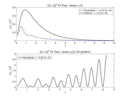
Figure 2: Simulation results for known $\tau_{u}$. Top: stability confirming the LMI results. Bottom: instability without predictor

5 Conclusion

We suggested a finite-dimensional observer-based control of the 1D heat equation under Neumann actuation, non-local measurement and fast-varying input/output delays. Reduced-order LMI stability conditions were derived. Classical predictors were used to enlarge the delays.

References

[1]
Z. Artstein.
Linear systems with delayed controls: a reduction.
IEEE Transactions on Automatic Control, 27(4):869–879, 1982.
[2]
M. J. Balas.
Finite-dimensional controllers for linear distributed parameter
systems: exponential stability using residual mode filters.
Journal of Mathematical Analysis and Applications,
133(2):283–296, 1988.
[3]
P. Christofides.
Nonlinear and Robust Control of PDE Systems: Methods and
Applications to transport reaction processes.
Springer, 2001.
[4]
R. Curtain.
Finite-dimensional compensator design for parabolic distributed
systems with point sensors and boundary input.
IEEE Transactions on Automatic Control, 27(1):98–104, 1982.
[5]
R. Curtain and K. Morris.
Transfer functions of distributed parameter systems: A tutorial.
Automatica, 45(5):1101–1116, 2009.
[6]
N. Espitia, I. Karafyllis, and M. Krstic.
Event-triggered boundary control of constant-parameter
reaction–diffusion PDEs: a small-gain approach.
Automatica, 128:109562, 2021.
[7]
E. Fridman.
Introduction to time-delay systems: analysis and control.
Birkhauser, Systems and Control: Foundations and Applications, 2014.
[8]
E. Fridman and A. Blighovsky.
Robust sampled-data control of a class of semilinear parabolic
systems.
Automatica, 48:826–836, 2012.
[9]
S. Ghantasala and N. El-Farra.
Active fault-tolerant control of sampled-data nonlinear distributed
parameter systems.
International Journal of Robust and Nonlinear Control,
22(1):24–42, 2012.
[10]
C. Harkort and J. Deutscher.
Finite-dimensional observer-based control of linear distributed
parameter systems using cascaded output observers.
International journal of control, 84(1):107–122, 2011.
[11]
W. Kang and E. Fridman.
Distributed sampled-data control of
Kuramoto-Sivashinsky equation.
Automatica, 95:514–524, 2018.
[12]
I. Karafyllis and M. Krstic.
Predictor feedback for delay systems: Implementations and
approximations.
Springer, 2017.
[13]
I. Karafyllis and M. Krstic.
Sampled-data boundary feedback control of 1-D parabolic
PDEs.
Automatica, 87:226–237, 2018.
[14]
R. Katz, I. Basre, and E. Fridman.