{textblock*}

(15mm,18mm) To appear in the Proceedings of the 20th European Control Conference (ECC), 2021.

Co-Design of Autonomous Systems: From Hardware Selection to Control Synthesis

Gioele Zardini, Andrea Censi, Emilio Frazzoli This work was supported by the Swiss National Science Foundation under NCCR Automation, grant agreement 51NF40_180545. The authors are with the Institute for Dynamic Systems and Control, ETH Zürich, Switzerland. {gzardini,acensi,efrazzoli}@ethz.ch.

Abstract

Designing cyber-physical systems is a complex task which requires insights at multiple abstraction levels. The choices of single components are deeply interconnected and need to be jointly studied. In this work, we consider the problem of co-designing the control algorithm as well as the platform around it. In particular, we leverage a monotone theory of co-design to formalize variations of the LQG control problem as monotone feasibility relations. We then show how this enables the embedding of control co-design problems in the higher level co-design problem of a robotic platform. We illustrate the properties of our formalization by analyzing the co-design of an autonomous drone performing search-and-rescue tasks and show how, given a set of desired robot behaviors, we can compute Pareto efficient design solutions.

I Introduction

Refer to caption — (a) A MDPI is a monotone relation between partially ordered sets (posets) of functionalities and resources.

Cyber-physical systems are composed of material parts, such as sensors, actuators and computing units, and software components, such as perception, planning, and control modules. Traditionally, the design optimization of such components is treated in a compartmentalized manner, assuming specific, fixed configurations for the parts of the system which are not object of the design exercise. However, the designs of both physical and software components are deeply interconnected and need to be jointly considered. Examples of the importance of a joint design of components range from power-constrained robot design [1, 2] to the design of fleets of autonomous vehicles which need to provide mobility services jointly with the existing urban transportation system [3, 4]. Open questions are: What is the simplest sensor which a robot can use to guarantee a specific performance in a given task? How will this choice affect computation? Which platform design minimizes the overall monetary cost?

In this work, we propose an approach for the co-design of the platform and its control system (Fig. 1(d)), with particular reference to robotics. While a broad theory to optimize the control of specific systems has been developed, there exists no formalism which allows to jointly design control strategies and the platforms on which they will be executed. This is an issue, since robotic platforms are typically not fixed, and components such as actuators, sensors and batteries are subject to continuous changes.

Related literature

Traditionally, researchers have been working on specific instances of the co-design of control, sensing and actuation [5, 6, 7, 8, 9, 10, 11, 12, 13, 14, 15, 16, 17, 18, 19, 20, 21, 22]. The author of [5] formalizes the optimal design of the robotic platform for serial manipulators, and a precise analysis of trade-offs in robot sensing and actuation for worst-case scenarios is provided in [6]. The authors of [7] and [8] propose approaches for the co-design of control algorithms and platforms, applied to lane keeping and HVAC systems, respectively, and [9, 10] focus on performance and security of cyber-physical systems. The problem of sensor selection typically cannot be solved in a closed form, but [11, 12] show that in particular cases, there is enough structure for efficient optimization. Specifically, the authors of [13] study the problem of sensing-constrained LQG control, providing examples of robotic tasks, and authors of [14] optimally select sensors to solve path planning problems. In [15], the authors propose an approach for optimal control with communication constraints and [16] provides a framework to jointly optimize sensor selection and control, by minimizing the information acquired by the sensor. An analysis of performance limits for robotic tasks parametrized by the complexity of the environment is given in [17]. Selection of sensors and actuators is studied in [18], where the authors optimize the design of the system with the goal of providing robust control for aeroservoelastic systems. Furthermore, [19] proposes an approach to optimize actuators placement in large-scale networks control, [20] studies computation-communication trade-offs and sensor selection for processing networks, and [22] gives a broad view of compositional cyber-physical system theories. In conclusion, to the best of our knowledge, existing design techniques for autonomous platforms are characterized by a fixed, problem-specific structure and do not allow to formalize and solve system co-design problems involving control synthesis.

Statement of contributions

In this work we show how to use a monotone theory of co-design to frame the design of LQG control strategies in the co-design problem of an entire robotic platform. First, we formulate (variations of) LQG control as a MDPI, characterized by feasibility relations between the control performance, accuracy, measurements’ and system’s noises. Second, we show how nuisances such as delays, digitalization and intermittent observations can be integrated in our formalism. The proofs for our results are available in Sections -B and -C. Finally, we showcase the advantages of our approach, considering the co-design problem of a mobile robot which needs to execute an idealized search-and-rescue task (Fig. 1(d)). We illustrate how, given the robot model and desired behaviors, we can formulate and answer several questions regarding the design of the robot.

II Monotone Co-Design Theory

We assume the reader to be familiar with basic concepts from order theory (listed in Section -A). A possible reference is [23]. In this section, we report the main concepts related to the mathematical theory of co-design [24, 25].

Definition 1 (MDPI).

Given the partially ordered sets (posets) ${\color[rgb]{0.0,0.5,0.0}\definecolor[named]{pgfstrokecolor}{rgb}{0.0,0.5,0.0}\mathcal{F}},{\color[rgb]{0.7,0.0,0.0}\definecolor[named]{pgfstrokecolor}{rgb}{0.7,0.0,0.0}\mathcal{R}}$ , representing functionalities and resources, respectively, we define a MDPI $d$ as a tuple $\langle\mathcal{I}_{d},\mathsf{prov},\mathsf{req}\rangle$ , where $\mathcal{I}_{d}$ is the set of implementations, and $\mathsf{prov}$ , $\mathsf{req}$ are functions mapping $\mathcal{I}_{d}$ to ${\color[rgb]{0.0,0.5,0.0}\definecolor[named]{pgfstrokecolor}{rgb}{0.0,0.5,0.0}\mathcal{F}}$ and ${\color[rgb]{0.7,0.0,0.0}\definecolor[named]{pgfstrokecolor}{rgb}{0.7,0.0,0.0}\mathcal{R}}$ , respectively:

{\color[rgb]{0.0,0.5,0.0}\definecolor[named]{pgfstrokecolor}{rgb}{0.0,0.5,0.0}\mathcal{F}}\xleftarrow{\mathsf{prov}}\mathcal{I}_{d}\xrightarrow{\mathsf{req}}{\color[rgb]{0.7,0.0,0.0}\definecolor[named]{pgfstrokecolor}{rgb}{0.7,0.0,0.0}\mathcal{R}}.

To each MDPI we associate a monotone map $\bar{d}$ given by

	$\displaystyle\bar{d}\colon{\color[rgb]{0.0,0.5,0.0}\definecolor[named]{pgfstrokecolor}{rgb}{0.0,0.5,0.0}\mathcal{F}}^{\mathrm{op}}\times{\color[rgb]{0.7,0.0,0.0}\definecolor[named]{pgfstrokecolor}{rgb}{0.7,0.0,0.0}\mathcal{R}}$	$\displaystyle\to\mathbb{P}({\mathcal{I}_{d}})$
	$\displaystyle\langle{\color[rgb]{0.0,0.5,0.0}\definecolor[named]{pgfstrokecolor}{rgb}{0.0,0.5,0.0}f}^{*},{\color[rgb]{0.7,0.0,0.0}\definecolor[named]{pgfstrokecolor}{rgb}{0.7,0.0,0.0}r}\rangle$	$\displaystyle\mapsto\{i\in\mathcal{I}_{d}\colon(\mathsf{prov}(i)\succeq_{{\color[rgb]{0.0,0.5,0.0}\definecolor[named]{pgfstrokecolor}{rgb}{0.0,0.5,0.0}\mathcal{F}}}{\color[rgb]{0.0,0.5,0.0}\definecolor[named]{pgfstrokecolor}{rgb}{0.0,0.5,0.0}f})\wedge(\mathsf{req}(i)\preceq_{{\color[rgb]{0.7,0.0,0.0}\definecolor[named]{pgfstrokecolor}{rgb}{0.7,0.0,0.0}\mathcal{R}}}{\color[rgb]{0.7,0.0,0.0}\definecolor[named]{pgfstrokecolor}{rgb}{0.7,0.0,0.0}r})\},$

where $(\cdot)^{\mathrm{op}}$ reverses the order of a poset. A MDPI is represented in diagrammatic form as in Fig. 1(a). The expression $\bar{d}({\color[rgb]{0.0,0.5,0.0}\definecolor[named]{pgfstrokecolor}{rgb}{0.0,0.5,0.0}f^{*}},{\color[rgb]{0.7,0.0,0.0}\definecolor[named]{pgfstrokecolor}{rgb}{0.7,0.0,0.0}r})$ returns the set of implementations $S\subseteq\mathcal{I}_{d}$ for which functionalities ${\color[rgb]{0.0,0.5,0.0}\definecolor[named]{pgfstrokecolor}{rgb}{0.0,0.5,0.0}f}$ are feasible with resources ${\color[rgb]{0.7,0.0,0.0}\definecolor[named]{pgfstrokecolor}{rgb}{0.7,0.0,0.0}r}$ .

Example 1 (Monotonicity).

Consider the MDPI of a battery (block in Fig. 1(d)) by means of the provided energy and the required cost and mass. If a set $S=d({\color[rgb]{0.0,0.5,0.0}\definecolor[named]{pgfstrokecolor}{rgb}{0.0,0.5,0.0}f}^{*},{\color[rgb]{0.7,0.0,0.0}\definecolor[named]{pgfstrokecolor}{rgb}{0.7,0.0,0.0}r})$ of batteries require ${\color[rgb]{0.7,0.0,0.0}\definecolor[named]{pgfstrokecolor}{rgb}{0.7,0.0,0.0}r}=\langle{\color[rgb]{0.7,0.0,0.0}\definecolor[named]{pgfstrokecolor}{rgb}{0.7,0.0,0.0}\text{mass}},{\color[rgb]{0.7,0.0,0.0}\definecolor[named]{pgfstrokecolor}{rgb}{0.7,0.0,0.0}\text{cost}}\rangle$ to provide ${\color[rgb]{0.0,0.5,0.0}\definecolor[named]{pgfstrokecolor}{rgb}{0.0,0.5,0.0}f}={\color[rgb]{0.0,0.5,0.0}\definecolor[named]{pgfstrokecolor}{rgb}{0.0,0.5,0.0}\text{energy}}$ , then they can also provide less energy ${\color[rgb]{0.0,0.5,0.0}\definecolor[named]{pgfstrokecolor}{rgb}{0.0,0.5,0.0}f^{\prime}}\preceq{\color[rgb]{0.0,0.5,0.0}\definecolor[named]{pgfstrokecolor}{rgb}{0.0,0.5,0.0}f}$ , i.e. $S^{\prime}\supseteq S$ . On the other hand, if one has more resources ${\color[rgb]{0.7,0.0,0.0}\definecolor[named]{pgfstrokecolor}{rgb}{0.7,0.0,0.0}r^{\prime\prime}}\succeq{\color[rgb]{0.7,0.0,0.0}\definecolor[named]{pgfstrokecolor}{rgb}{0.7,0.0,0.0}r}$ , the new set of batteries will at least still provide ${\color[rgb]{0.0,0.5,0.0}\definecolor[named]{pgfstrokecolor}{rgb}{0.0,0.5,0.0}f}$ , i.e. $S^{\prime\prime}\supseteq S$ .

Definition 2.

Given a MDPI $d$ , we define monotone maps $h_{d}\colon{\color[rgb]{0.0,0.5,0.0}\definecolor[named]{pgfstrokecolor}{rgb}{0.0,0.5,0.0}\mathcal{F}}\to\mathcal{A}{\color[rgb]{0.7,0.0,0.0}\definecolor[named]{pgfstrokecolor}{rgb}{0.7,0.0,0.0}\mathcal{R}}$ , mapping a functionality to the minimum antichain of resources providing it, and $h_{d}^{\prime}\colon{\color[rgb]{0.7,0.0,0.0}\definecolor[named]{pgfstrokecolor}{rgb}{0.7,0.0,0.0}\mathcal{R}}\to\mathcal{A}{\color[rgb]{0.0,0.5,0.0}\definecolor[named]{pgfstrokecolor}{rgb}{0.0,0.5,0.0}\mathcal{F}}$ , mapping a resource to the maximum antichain of functionalities provided by it. To solve MDPIs we find these maps, relying on Kleene’s fixed point theorem [24].

Individual MDPIs can be composed in several ways to form a co-design problem (Fig. 3). Series composition describes the case in which the functionality of a MDPI becomes the resource of another MDPI. For instance, the computation power provided by a computer is required by algorithm implementations. The relation “ $\preceq$ ” appearing in Fig. 3 represents a co-design constraint: The resource one component requires has to be at most the one provided by another component. Parallel composition corresponds to processes happening together. Finally, loop composition describes feedback.¹¹1It can be proved that the formalization of feedback makes the category of MDPIs a traced monoidal category [26]. Composition operations preserve monotonicity and thus all related algorithmic properties [24].

(a) Series composition.

(b) Parallel composition.

Figure 3: MDPIs can be composed in different ways.

III Continuous-time LQG control as a MDPI

Background on LQG control

First, we recall the definition of infinite-horizon LQG control.

Definition 3 (Continuous-time LQG control).

Given the continuous-time stochastic dynamics

	$\displaystyle\mathrm{d}\bm{x}_{t}$	$\displaystyle=\mathbf{A}\bm{x}_{t}\mathrm{d}t+\mathbf{B}\bm{u}_{t}\mathrm{d}t+\mathbf{E}\mathrm{d}\bm{w}_{t}$
	$\displaystyle\mathrm{d}\bm{y}_{t}$	$\displaystyle=\mathbf{C}\bm{x}_{t}\mathrm{d}t+\mathbf{G}\mathrm{d}\bm{v}_{t},$

where $\bm{v}_{t}$ and $\bm{w}_{t}$ are two standard Brownian processes, let $\mathbf{A},\mathbf{B},\mathbf{C}$ , $\mathbf{E}$ , $\mathbf{G}$ be matrices of compatible dimensions and $\mathbf{W}=\mathbf{E}\mathbf{E}^{*}$ , $\mathbf{V}=\mathbf{G}\mathbf{G}^{*}$ be the effective noise covariances. The continuous-time infinite-horizon LQG problem consists of finding a control law $\bm{u}^{\star}$ minimizing the quadratic cost

J=\textstyle{\lim_{T\to\infty}}\frac{1}{T}\mathbb{E}\{\smallint_{0}^{T}\left(\left(\bm{x}_{t}^{\intercal}\mathbf{Q}\bm{x}_{t}\right)+\left(\bm{u}_{t}^{\intercal}\mathbf{R}\bm{u}_{t}\right)\right)\mathrm{d}t\},

with $\mathbf{Q}\in\mathcal{P}$ , $\mathbf{R}\in\mathcal{P}^{+}$ , where $\mathcal{P}^{+}$ ( $\mathcal{P}$ ) is the set of positive definite (positive semi-definite) matrices.

Remark.

In this work we use the Hermitian matrices poset $\langle\mathcal{M}^{n},\preceq\rangle$ . Given two Hermitian matrices of order $n$ $\mathbf{A},\mathbf{B}\in\mathcal{M}^{n}$ , we have $\mathbf{A}\preceq\mathbf{B}\Leftrightarrow(\mathbf{B}-\mathbf{A})\in\mathcal{P}^{+}$ . These matrices have real eigenvalues, which we can think of as axis lengths of ellipsoids. Order is given by ellipsoid inclusion.

Lemma 1.

The optimal control law for the LQG problem in Def. 3 is $\bm{u}_{t}^{\star}=-\mathbf{K}\hat{\bm{x}}_{t}=-\mathbf{R}^{-1}\mathbf{B}^{*}\bar{\mathbf{S}}\hat{\bm{x}}_{t}$ , where $\hat{\bm{x}}_{t}$ is the unbiased minimum-variance estimate of $\bm{x}_{t}$ given previous measurements and $\bar{\mathbf{S}}\in\mathcal{P}^{+}$ solves the Riccati equation

\mathbf{SA}+\mathbf{A}^{*}\mathbf{S}-\mathbf{SBR}^{-1}\mathbf{B}^{*}\mathbf{S}+\mathbf{Q}=\mathbf{0}.

(1)

The minimum cost $J^{\star}$ achieved by the optimal control is²²2Note that [27] contains a typo at p.188 (one extra $\mathbf{V}^{-1}$ factor). Instead, [28] has a cleaner derivation and exposition.:

	$\displaystyle J^{\star}$	$\displaystyle=\mathsf{Tr}\left(\bar{\mathbf{S}}\bar{\mathbf{\Sigma}}\mathbf{C}^{*}\mathbf{V}^{-1}\mathbf{C}\bar{\mathbf{\Sigma}}+\bar{\mathbf{\Sigma}}\mathbf{Q}\right)$
		$\displaystyle=\mathsf{Tr}\left(\bar{\mathbf{\Sigma}}\bar{\mathbf{S}}\mathbf{BR}^{-1}\mathbf{B}^{*}\bar{\mathbf{S}}+\bar{\mathbf{S}}\mathbf{W}\right),$

where $\bar{\mathbf{\Sigma}}\in\mathcal{P}^{+}$ is the solution of the Riccati equation

\mathbf{A\Sigma}+\mathbf{\Sigma A}^{*}-\mathbf{\Sigma C}^{*}\mathbf{V}^{-1}\mathbf{C\Sigma}+\mathbf{W}=\mathbf{0}.

(2)

(a) LQG digital control with observation and computation delays, sampling and ZOH.

(b) Diagrammatic representation of co-design theorems.

Figure 4: (a) We consider the case of LQG control first in the continuous-time and then in the digital case. We highlight the monotonicity in several nuisances in the problem. For instance, if the probability of dropping observations increases, the tracking error will not decrease. These properties are summarized diagrammatically in (b), which is the graphical representation of the feasibility relations presented in this work.

Co-design formalization

To formalize the LQG control problem as a MDPI, we first define two performance metrics. From a continuous-time LQG problem, we define the stationary tracking error $P_{\mathrm{track}}$ and control effort $P_{\mathrm{effort}}$ :

P_{\mathrm{track}}=\textstyle{\lim_{t\to\infty}}\mathbb{E}\{\bm{x}_{t}^{\intercal}\mathbf{Q}\bm{x}_{t}\},\ P_{\mathrm{effort}}=\textstyle{\lim_{t\to\infty}}\mathbb{E}\{\bm{u}_{t}^{\intercal}\mathbf{R}\bm{u}_{t}\}.

We are now ready to state the first central result of this work.

Theorem 1.

The LQG problem of Def. 3 can be formulated and solved as a MDPI with diagrammatic form as in Fig. 1(b).

To prove Theorem 1, we show that there exists a MDPI as in Def. 1, relating functionalities ${\color[rgb]{0.0,0.5,0.0}\definecolor[named]{pgfstrokecolor}{rgb}{0.0,0.5,0.0}\mathbf{V}},{\color[rgb]{0.0,0.5,0.0}\definecolor[named]{pgfstrokecolor}{rgb}{0.0,0.5,0.0}\mathbf{W}}$ and resources ${\color[rgb]{0.7,0.0,0.0}\definecolor[named]{pgfstrokecolor}{rgb}{0.7,0.0,0.0}P_{\mathrm{track}}},{\color[rgb]{0.7,0.0,0.0}\definecolor[named]{pgfstrokecolor}{rgb}{0.7,0.0,0.0}P_{\mathrm{effort}}}$ . First, by writing ${\color[rgb]{0.7,0.0,0.0}\definecolor[named]{pgfstrokecolor}{rgb}{0.7,0.0,0.0}P_{\mathrm{track}}}$ and ${\color[rgb]{0.7,0.0,0.0}\definecolor[named]{pgfstrokecolor}{rgb}{0.7,0.0,0.0}P_{\mathrm{effort}}}$ explicitly (Lemma 2), we prove their monotonicity with respect to cost weighting (Lemma 3). Second, we show the monotone relation characterizing the MDPI (Lemma 4 and Lemma 5).

Lemma 2.

The metrics $P_{\mathrm{track}}$ and $P_{\mathrm{effort}}$ can be written as

	$\displaystyle\textstyle{\lim_{t\to\infty}}\mathbb{E}\{\bm{x}_{t}^{\intercal}\mathbf{Q}_{0}\bm{x}_{t}\}$	$\displaystyle=\mathsf{Tr}\left(\mathbf{Q}_{0}\left(\mathbf{\Sigma}+\mathbf{F}\right)\right),$
	$\displaystyle\textstyle{\lim_{t\to\infty}}\mathbb{E}\{\bm{u}_{t}^{\intercal}\mathbf{R}_{0}\bm{u}_{t}\}$	$\displaystyle=\mathsf{Tr}\left(\mathbf{S}\mathbf{B}^{*}\mathbf{R}^{-1}\mathbf{R}_{0}\mathbf{R}^{-1}\mathbf{B}\mathbf{S}\mathbf{F}\right),$

where $\mathbf{\Sigma}$ solves 2, $\mathbf{F}$ solves the Lyapunov equation

\left(\mathbf{A}-\mathbf{B}\mathbf{K}\right)\mathbf{F}+\mathbf{F}\left(\mathbf{A}-\mathbf{B}\mathbf{K}\right)^{*}+\mathbf{L}\mathbf{V}\mathbf{L}^{*}=\mathbf{0},

(3)

$\mathbf{S}$ solves 1 and $\mathbf{L}=\mathbf{\Sigma}\mathbf{C}^{*}\mathbf{V}^{-1}$ is the Kalman gain.

Given explicit forms, we can now show that they are characterized by monotonic relations.

Lemma 3.

Let $\mathbf{Q}(\alpha)=\alpha\mathbf{Q}_{0}$ and $\mathbf{R}(\alpha)=\frac{1}{\alpha}\mathbf{R}_{0}$ , $\alpha\in\mathbb{R}_{+}$ . Let $\bm{u}^{\star}(\alpha)$ be the solution of the LQG problem with $\mathbf{Q}(\alpha)$ and $\mathbf{R}(\alpha)$ . Then, under optimal control one has:

•

$P_{\mathrm{track}}(\alpha)$ is decreasing with $\alpha$ increasing.
•

$P_{\mathrm{effort}}(\alpha)$ is increasing with $\alpha$ increasing.

Intuitively, by increasing $\alpha$ we increase the penalty for the tracking error of the control. For this reason, $P_{\mathrm{track}}$ decreases and $P_{\mathrm{effort}}$ increases. We now want to assess the effect of the system and observation noises on the optimal control.

Lemma 4.

The solution of 2 is monotonic in $\mathbf{V}$ and $\mathbf{W}$ , i.e., $\langle\mathbf{V},\mathbf{W}\rangle\preceq\langle\mathbf{V}^{\prime},\mathbf{W}^{\prime}\rangle\Rightarrow\mathbf{\Sigma}(\mathbf{V},\mathbf{W})\preceq\mathbf{\Sigma}(\mathbf{V}^{\prime},\mathbf{W}^{\prime})$ .

Lemma 5.

Consider the situation of Lemma 3:

•

Fix $P_{\mathrm{track}}$ . $P_{\mathrm{effort}}$ is monotonic in $\mathbf{W}$ and in $\mathbf{V}$ .
•

Fix $P_{\mathrm{effort}}$ . $P_{\mathrm{track}}$ is monotonic in $\mathbf{W}$ and in $\mathbf{V}$ .

This shows that the more uncertain the observations and the system dynamics are, the larger the control effort and tracking error will be, and concludes the proof of Theorem 1.

The presented MDPI precisely assesses the feasibility relation between control effort, tracking error, system noise, and the observation noise. This MDPI can be manipulated by taking the “op” of a quantity (Def. 1), and moving it on the other side of the diagram. For instance, we can think of the observation noise as resource, by switching its meaning to information (i.e., from noise to information matrix).

Dealing with delays

We now show the ability of our formalism to capture the influence of delays on the system.

Theorem 2.

A continuous-time LQG problem with observation and computation delays ( $d_{\mathrm{obs}}$ , $d_{\mathrm{comp}}$ ) can be formulated and solved as a MDPI with diagrammatic as in Fig. 1(c).

To establish the effect of a nuisance, we follow what we call the substitution principle. If in the case in which the nuisance was “lower” the controller could simulate a “higher” nuisance, then we have monotonicity. If we had a smaller delay, we could simulate a larger one by adding it artificially. Hence, control effort and tracking error of the optimal control strategy cannot decrease with larger delay.

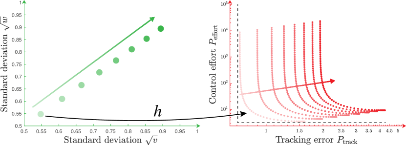
Visualization via Pareto fronts

We want to give a visual interpretation of the presented results. For the scalar case of Def. 3 we can derive $P_{\mathrm{track}}$ and $P_{\mathrm{effort}}$ in closed-form:

	$\displaystyle P_{\mathrm{track}}(q_{0})$	$\displaystyle=q_{0}\left(\bar{\sigma}+\frac{\bar{(\sigma}c)^{2}}{2v\sqrt{a^{2}+\alpha^{2}q_{0}b^{2}/r_{0}}}\right),$
	$\displaystyle P_{\mathrm{effort}}(r_{0})$	$\displaystyle=\frac{r_{0}\bar{\sigma}^{2}c^{2}}{2b^{2}v}\frac{\left(a+\sqrt{a^{2}+\alpha^{2}b^{2}q_{0}/r_{0}}\right)^{2}}{\sqrt{a^{2}+\alpha^{2}b^{2}q_{0}/r_{0}}},$

where variables are in lower case since they represent scalar quantities. We can compute their limits, by fixing $v$ and $w$ :

	$\displaystyle\lim_{\alpha\to 0}P_{\mathrm{track}}(q_{0})$	$\displaystyle=q_{0}\left(\bar{\sigma}+\frac{(\bar{\sigma}c)^{2}}{2va}\right),\lim_{\alpha\to\infty}P_{\mathrm{track}}(q_{0})=q_{0}\bar{\sigma},$
	$\displaystyle\lim_{\alpha\to 0}P_{\mathrm{effort}}(r_{0})$	$\displaystyle=\frac{2r_{0}a(c\bar{\sigma})^{2}}{{b^{2}v}},\lim_{\alpha\to\infty}P_{\mathrm{effort}}(r_{0})=\infty.$

We can plot instances of the Pareto front $\langle{\color[rgb]{0.7,0.0,0.0}\definecolor[named]{pgfstrokecolor}{rgb}{0.7,0.0,0.0}P_{\mathrm{track}}},{\color[rgb]{0.7,0.0,0.0}\definecolor[named]{pgfstrokecolor}{rgb}{0.7,0.0,0.0}P_{\mathrm{effort}}}\rangle$ (Fig. 1(e)). This is the query in which we “fix functionalities and minimize resources”, where the Pareto fronts represent the best achievable control performances, given specific $v$ and $w$ . Alternatively, we could ask to “fix resources and maximize functionalities”. This is the query in which we fix ${\color[rgb]{0.7,0.0,0.0}\definecolor[named]{pgfstrokecolor}{rgb}{0.7,0.0,0.0}P_{\mathrm{track}}}$ and ${\color[rgb]{0.7,0.0,0.0}\definecolor[named]{pgfstrokecolor}{rgb}{0.7,0.0,0.0}P_{\mathrm{effort}}}$ , and observe a Pareto front of system and observation noises at which the given performance can be provided. Monotonicity is easy to see. By choosing $\langle{\color[rgb]{0.0,0.5,0.0}\definecolor[named]{pgfstrokecolor}{rgb}{0.0,0.5,0.0}v_{1}},{\color[rgb]{0.0,0.5,0.0}\definecolor[named]{pgfstrokecolor}{rgb}{0.0,0.5,0.0}w_{1}}\rangle\preceq\langle{\color[rgb]{0.0,0.5,0.0}\definecolor[named]{pgfstrokecolor}{rgb}{0.0,0.5,0.0}v_{2}},{\color[rgb]{0.0,0.5,0.0}\definecolor[named]{pgfstrokecolor}{rgb}{0.0,0.5,0.0}w_{2}}\rangle$ (i.e., ${\color[rgb]{0.0,0.5,0.0}\definecolor[named]{pgfstrokecolor}{rgb}{0.0,0.5,0.0}v_{1}}\leq{\color[rgb]{0.0,0.5,0.0}\definecolor[named]{pgfstrokecolor}{rgb}{0.0,0.5,0.0}v_{2}}$ and ${\color[rgb]{0.0,0.5,0.0}\definecolor[named]{pgfstrokecolor}{rgb}{0.0,0.5,0.0}w_{1}}\leq{\color[rgb]{0.0,0.5,0.0}\definecolor[named]{pgfstrokecolor}{rgb}{0.0,0.5,0.0}w_{2}}$ ), we see that both ${\color[rgb]{0.7,0.0,0.0}\definecolor[named]{pgfstrokecolor}{rgb}{0.7,0.0,0.0}P_{\mathrm{track}}}$ and ${\color[rgb]{0.7,0.0,0.0}\definecolor[named]{pgfstrokecolor}{rgb}{0.7,0.0,0.0}P_{\mathrm{effort}}}$ increase, and hence that the Pareto fronts dominate each other.

IV Digital LQG control as a MDPI

Digital LQG control

We define the infinite-horizon discrete-time LQG control problem.

Definition 4 (Discrete-time LQG control).

Consider the discrete-time stochastic dynamics

	$\displaystyle\bm{x}_{k}$	$\displaystyle={\mathbf{A}}_{\mathrm{d}}\bm{x}_{k}+{\mathbf{B}}_{\mathrm{d}}\bm{u}_{k}+{\mathbf{E}}_{\mathrm{d}}\bm{w}_{k}$
	$\displaystyle\bm{y}_{k}$	$\displaystyle={\mathbf{C}}_{\mathrm{d}}\bm{x}_{k}+{\mathbf{G}}_{\mathrm{d}}\bm{v}_{k},$

where $\bm{w}_{k}$ and $\bm{v}_{k}$ are two standard Brownian processes and ${\mathbf{W}}_{\mathrm{d}}=\mathbf{E}\mathbf{E}^{*}$ , ${\mathbf{V}}_{\mathrm{d}}=\mathbf{G}\mathbf{G}^{*}$ the noise covariances. The discrete-time infinite-horizon LQG problem consists of finding a control law $\bm{u}^{\star}$ which minimizes the quadratic cost

{J}_{\mathrm{d}}=\textstyle{\lim_{N\to\infty}}\frac{1}{N}\mathbb{E}\{\sum_{i=0}^{N-1}\left(\bm{x}_{i}^{\intercal}{\mathbf{Q}}_{\mathrm{d}}\bm{x}_{i}+\bm{u}_{i}^{\intercal}{\mathbf{R}}_{\mathrm{d}}\bm{u}_{i}\right)\},

where ${\mathbf{Q}}_{\mathrm{d}}\in\mathcal{P}$ , ${\mathbf{R}}_{\mathrm{d}}\in\mathcal{P}^{+}$ .

We want to show that the relations found in Section III hold for the case of digital LQG control, where we want to control a continuous-time system using a digital controller.

Lemma 6.

Consider a continuous-time LQG problem, where observations are sampled with period $\delta$ and processed by a digital controller to produce a control input (Fig. 4(a)). The input is reconstructed using ZOH with period $\delta$ . We can find:

	$\displaystyle{\mathbf{A}}_{\mathrm{d}}$	$\displaystyle=e^{\mathbf{A}\delta},{\mathbf{B}}_{\mathrm{d}}=\smallint_{0}^{\delta}e^{\mathbf{A}s}\mathbf{B}\mathrm{d}s,{\mathbf{C}}_{\mathrm{d}}=\mathbf{C},{\mathbf{Q}}_{\mathrm{d}}=\smallint_{0}^{\delta}e^{\mathbf{A}^{\intercal}s}\mathbf{Q}e^{\mathbf{A}s}\mathrm{d}s,$
	$\displaystyle{\mathbf{R}}_{\mathrm{d}}$	$\displaystyle=\smallint_{0}^{\delta}((\smallint_{0}^{s}e^{\mathbf{A}t}\mathbf{B}\mathrm{d}t)\mathbf{Q}(\smallint_{0}^{s}e^{\mathbf{A}t}\mathbf{B}\mathrm{d}t)^{\intercal}+\mathbf{R})\mathrm{d}s.$

such that the optimal cost of this controller coincides with the optimal cost ${J}_{\mathrm{d}}$ in Def. 4.

Define the stationary digital tracking error and control effort:

P_{\mathrm{track}}^{\mathrm{d}}=\lim_{k\to\infty}\mathbb{E}\{\bm{x}_{k}^{\intercal}\mathbf{Q}\bm{x}_{k}\},~{}P_{\mathrm{effort}}^{\mathrm{d}}=\lim_{k\to\infty}\mathbb{E}\{\bm{u}_{k}^{\intercal}\mathbf{R}\bm{u}_{k}\}.

We can now formulate Theorem 1 for the discrete-time case.

Theorem 3.

The digital LQG problem in Lemma 6 with fixed sampling period $\delta$ can be formulated and solved as a MDPI with diagrammatic form as in Fig. 1(b).

The proof is analogous to the one of Theorem 1. Theorem 3 allows us to interconnect LQG control problems as MDPIs in the co-design diagram of a real robotic platform.

Effect of sampling period and intermittent observations

We now assess the impact of sampling period and intermittent observations [29, 30] on digital LQG control.

Definition 5 (LQG with intermittent observations).

The LQG problem with intermittent observations differs from the original problem by the observations $\bm{y}_{k}^{\prime}=\gamma_{k}\bm{y}_{k}$ , where $\gamma_{k}\in\{0,1\}$ is a random sequence.

Theorem 4.

The digital LQG problem given in Fig. 4(a) with delay of the form $\delta=2^{n}\delta_{0}$ can be formulated and solved as a MDPI with diagrammatic form as in Fig. 4(b).

To prove both cases, we can use the substitution principle. Assuming a sampling period $\delta=2^{n}\delta_{0}$ , $P_{\mathrm{track}}$ and $P_{\mathrm{effort}}$ are monotonic with $n$ .³³3Note that using $\delta$ of this form corresponds to the case where the information available is a subset decreasing with $n$ . We are not stating this result in general. This would require a deeper discussion and several assumptions about the system (e.g., about oscillatory behavior). This is an open problem [31, 32] and we leave its extensive treatment to future work. On the other hand, if the controller is given a set of observations, it can simulate having less (i.e., an higher drop probability $p$ ), by artificially deleting selected observations. Therefore, the control effort and tracking error cannot decrease with increasing $p$ .

Discussion

Theorems 1, 2, 3 and 4 show how to frame and solve variations of LQG control problems as MDPIs. In particular, the results provide an interface to include control synthesis in the robot co-design problem. Note that the theory and results generalize to the case of parameter uncertainty [33]. In the next section we show how this new perspective allows one to solve complex robot co-design problems, capturing heterogeneous abstraction levels within a unified framework.

V Co-design of an autonomous drone

Figure 5: Data-flow diagram for an autonomous system.

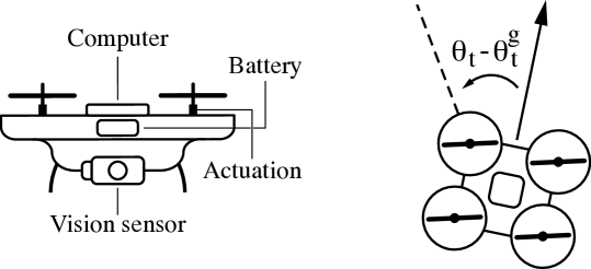
In this section we show the ability of the proposed formalism to capture LQG control synthesis together with practical aspects related to robot design, such as sensor, actuation and computer selection. We consider a sensor-based navigation task for an autonomous drone (Fig. 2). The drone must reach a goal and it is guided by a vision sensor, used as a bearing sensor, needed to detect the relative direction of the goal.

V-A System modeling

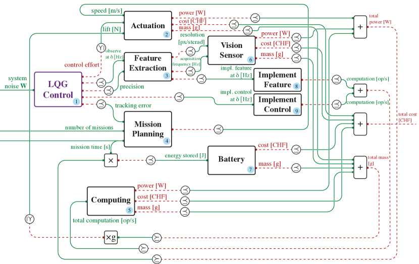
To understand the co-design approach, we need to distinguish logical dependencies and data-flow. While the diagram provided in Fig. 5 describes the system’s data-flow, the co-design diagram in Fig. 1(d) formalizes logical dependencies through functional decomposition. We now present the single MDPIs composing the co-design diagram, together with an explanation on how to obtain the models.

Block LQG Control: Given the task of aligning itself with the goal, we define the state of the robot as $\langle\theta_{t},\omega_{t}\rangle$ , where $\theta_{t}$ is its heading and $\omega_{t}$ its angular speed. The heading of the goal at time $t$ is denoted by $\theta_{t}^{\mathrm{g}}$ . The control is the resulting torque $\tau_{t}$ . The dynamics of the heading are given by the differential equations $\mathrm{d}\theta_{t}=\omega_{t}\mathrm{d}t$ , $\mathrm{d}\omega_{t}=\frac{\tau_{t}}{I}\mathrm{d}t+\mathrm{d}w_{t}$ , where $I$ is the moment of inertia of the drone about its rotational axis, and $w_{t}$ is a Brownian process with intensity ${\color[rgb]{0.0,0.5,0.0}\definecolor[named]{pgfstrokecolor}{rgb}{0.0,0.5,0.0}\sigma_{w}^{2}}$ . We assume Gaussian observations of the relative bearing of drone and goal $y_{t}=(\theta_{t}-\theta_{t}^{\mathrm{g}})+v_{t}$ , where $v_{t}$ is white Gaussian noise with intensity ${\color[rgb]{0.7,0.0,0.0}\definecolor[named]{pgfstrokecolor}{rgb}{0.7,0.0,0.0}\sigma_{v}^{2}}$ , describing measurement uncertainty. Assuming that the goal is far away, $\theta_{t}^{\mathrm{g}}$ is approximately constant, and w.l.o.g. we can assume it to be 0 ( $y_{t}=\theta_{t}+v_{t}$ ). We pose the stationary problem of minimizing the objective $\textstyle{\lim_{T\to\infty}}\frac{1}{T}\smallint_{0}^{T}\left(\alpha q_{0}\theta_{t}^{2}+\frac{r_{0}}{\alpha}\tau_{t}^{2}\right)\mathrm{d}t.$ This is a LQG problem with $\mathbf{Q}=\text{diag}(0,\alpha q_{0})$ , $\mathbf{R}=r_{0}/\alpha$ , for the continuous-time system given by the system matrices:

	$\displaystyle\mathbf{A}$	$\displaystyle=\begin{bmatrix}0&1\\ 0&0\end{bmatrix},\quad\mathbf{B}=\frac{1}{I}\begin{bmatrix}0\\ 1\end{bmatrix},\quad\mathbf{C}=\begin{bmatrix}1&0\end{bmatrix},$
	$\displaystyle\mathbf{W}$	$\displaystyle=\begin{bmatrix}0&0\\ 0&\sigma_{w}^{2}/I\end{bmatrix},\quad\mathbf{V}=\sigma_{v}^{2}.$

As shown in Section III, we can formalize this as a MDPI , which provides stability of the system up to a given system noise, requiring observations at a specific frequency and with given precision. The control law has to be implemented at a given frequency, resulting in specific control effort and tracking error. Implementations are given by the different cost weights, parametrized by $\alpha$ . Obtaining the model: As explained in Section III, the MDPI can be obtained by solving specific Riccati equations via numerical simulations.

Block Vision Sensor: The observations required by the control block are provided by a vision sensor at a given frequency and with a specific resolution. Such sensors have a cost, mass and power consumption. Obtaining the model: This is obtained from sensor catalogues (e.g., cameras).

Block Feature Extraction: Sensor measurements are processed by a feature extraction algorithm , providing the LQG control MDPI with observations at a certain frequency and accuracy, limited by sensor properties. Obtaining the model: This can be obtained by answering photogrammetry questions such as “what resolution is needed to achieve a certain detection accuracy?”

Blocks Algorithms Implementation: Given the above, we need to implement the control and feature detection algorithms , . Each of these is a MDPI, characterized by a catalogue of algorithms, each operating at a specific frequency and requiring computation power. Obtaining the model: This can be obtained via benchmarking. An example is given by SLAMBench [34].

Block Computing: The processes require computation power, provided by a computing unit . Each computing unit has a cost, mass, and requires power. Obtaining the model: We can model this via computer catalogues.

Block Actuation: The total mass of the system is lifted thanks to actuation , which provides lift, control effort and speed by requiring cost, mass and power. Obtaining the model: Models can be obtained from catalogues. For instance, power consumption can be modeled as a monotone function of lift and control effort, as in [24].

Block Battery: A battery provides energy to the system, requiring cost and mass. Obtaining the model: Different battery technologies can be extracted from catalogues [24].

Block Mission Planning: Finally, a mission planning block evaluates the performance of the system, measured by tracking error, the mission time, the number of missions and the detected drone speed. Obtaining the model: This is a simple list of requirements for specific scenarios.

Composing the full diagram

The single MDPIs presented in the previous paragraph are interconnected to form a co-design diagram (Fig. 1(d)) as follows. First, the total power required by the system arises from the sum of the power required by actuation, by the sensors and by the computing unit. Given the mission time, one can determine the energy which needs to be provided by the battery. This is the first feedback loop in the co-design diagram. Second, the computation required by both the control and feature extraction implementations needs to be provided by the computing unit (second loop). Third, the mass of the system is given by the masses of the sensors, battery, actuators and computing unit, and determines the lift needed from actuation (third loop). The number of loops provides an upper bound for the complexity of the solution algorithm [24, Proposition 5]. In particular, the solver will create a chain in the poset of antichains of $\bar{\mathbb{R}}_{\geq 0}^{3}$ , where the latter represents the poset containing the three resources which are fed back.

V-B Co-Design results

We now show how the proposed framework is able to solve the co-design problem of an autonomous drone, co-designing the controller synthesis together with the rest of the platform. We consider the MDPI reported in Fig. 1(d) and provide design insights in terms of cost, power consumption, tracking error, missions duration and number of missions.⁴⁴4The solver, based on a formal language, is available at codesign.science. We list the design variables in Table I. Specifically, they include the selection of sensors, control parameters, battery technologies, computing units and actuators. In the following, we bound the system noise and fix $q_{0}=r_{0}=1$ , to propose a sample of design insights that the framework can produce.

Remark.

The following results have to be understood qualitatively, not quantitatively: we contribute in the formalization of meta-models and interfaces, not in the numbers. We look forward to working with experts to get adequate data.

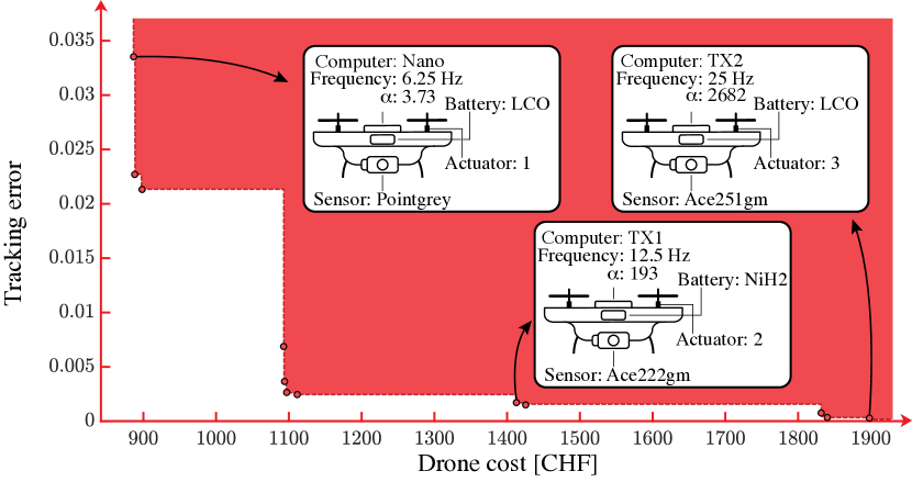
Cost and performance trade-off (Fig. 6(a))

We query the optimal design solutions which enable the drone to perform 5,000 missions lasting 40 minutes (Fig. 6(a)). The red dots represent the elements belonging to the antichain of optimal design solutions, expressed in terms of the platform cost and the tracking error. The solutions are not comparable, since no instance leads simultaneously to lower cost and tracking error. The upper set of resources (not necessarily optimal, but making the MDPI feasible) is given in solid red. We report implementations corresponding to specific optimal solutions. As can be gathered from Fig. 6(a), a budget increase for the drone reduces the tracking error. For instance, an investment from 900 CHF to 1,100 CHF reduces the tracking error by 90 %. On the other hand, a 27 % investment from 1,100 CHF to 1,400 CHF only reduces the tracking error by 5 %.

Power and performance trade-off (Fig. 6(b))

The optimization objectives can be quickly modified, without affecting the way the solution is obtained. For instance, we query the co-design framework in a similar way, now looking at the trade-offs between power consumption and tracking error for the case in which the drone must complete 1,000 missions lasting 10 minutes (Fig. 6(b)). When more power is available, better sensors and more performing computers, batteries and actuators can be used, reducing the tracking error.

Monotonicity of the drone MDPI (Fig. 6(c))

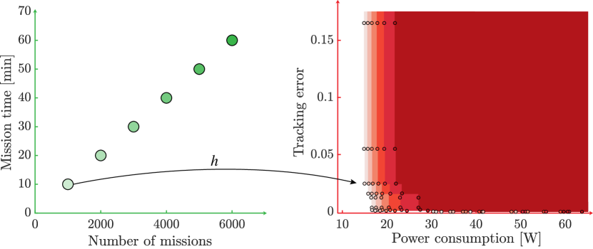
We consider increasing mission time and number of missions and assess the evolution in trade-offs in platform power consumption and tracking error. Fig. 6(c) shows multiple co-design queries. In particular, for each functionality (left plot), we compute the map $h$ , which maps a functionality to the minimum antichain of resources which provide it (Def. 2). Monotonicity can be seen in the dominance of subsequent Pareto fronts (right plot), illustrated in increasing red tonality.

Variable	Options	Source
Actuators	Type 1, 2, 3	[24]
Computer	RaspPi 4B, Jetson Nano/TX1/TX2	[35]
Control	0.2-50.0 Hz, $\alpha\in[10^{-4},10^{4}]$	-
Sensor	Basler Ace251gm/222gm/13gm/7gm/5gm/15um	[36]
	Flir Pointgrey/Blackfly/BlackflyBoard	[37]
Battery	LCO, LFP, LiPo, LMO, NiCad, NiH2, NiMH, SLA	[24]

TABLE I: Variables, options and sources for the drone co-design problem.

VI Conclusions

We considered the co-design of robotic platforms and linear control systems steering them. We have shown how to frame LQG control problems in a monotone theory of co-design, framing them as monotone feasibility relations (MDPIs). The approach guarantees modularity and compositionality, allowing us to model complex, interconnected systems and to capture heterogeneous design abstraction levels, ranging from control synthesis to hardware selection.

Outlook

This work fits in our vision of compositional robotics, where we want to describe and co-design robots all the way from signals characterising a single component [38] to networks and fleet effects [39]. We want to leverage compositionality properties of our framework to interconnect the co-design problem of a robot in the co-design problem of an urban robot-enabled mobility system, to assess how local trade-offs influence fleet-level operations [40]. Furthermore, we want to extend the proposed studies to the synthesis of more complex control structures.

Acknowledgments

We thank Dr. Fuller, Dr. Bonalli, Dr. Tanaka, Mr. Lanzetti, Mr. Zanardi, and Ms. Monti.

-A Background on orders

Definition 6 (Poset).

A poset is a tuple $\langle P,\preceq_{P}\rangle$ , where $P$ is a set and $\preceq_{P}$ is a partial order, defined as a reflexive, transitive, and antisymmetric relation.

Definition 7 (Opposite of a poset).

The opposite of a poset $\langle P,\preceq_{P}\rangle$ is the poset $\langle P^{\mathrm{op}},\preceq_{P}^{\mathrm{op}}\rangle$ , which has the same elements as $P$ , and the reverse ordering.

Definition 8 (Product poset).

Let $\langle P,\preceq_{P}\rangle$ and $\langle Q,\preceq_{Q}\rangle$ be posets. Then, $\langle P\times Q,\preceq_{P\times Q}\rangle$ is a poset with

\langle p_{1},q_{1}\rangle\preceq_{P\times Q}\langle p_{2},q_{2}\rangle\Leftrightarrow(p_{1}\preceq_{P}p_{2})\wedge(q_{1}\preceq_{Q}q_{2}).

This is called the product poset of $\langle P,\preceq_{P}\rangle$ and $\langle Q,\preceq_{Q}\rangle$ .

Definition 9 (Monotonicity).

A map $f\colon P\rightarrow Q$ between two posets $\langle P,\preceq_{P}\rangle$ , $\langle Q,\preceq_{Q}\rangle$ is monotone iff $x\preceq_{P}y$ implies $f(x)\preceq_{Q}f(y)$ . Monotonicity is compositional.

-B Proofs for Section III

Proof of Lemma 2.

With $\bm{e}_{t}=\bm{x}_{t}-\hat{\bm{x}}_{t}$ estimation error one has:

	$\displaystyle\lim_{t\to\infty}\mathbb{E}\{\bm{x}_{t}^{\intercal}\mathbf{Q}_{0}\bm{x}_{t}\}$	$\displaystyle=\lim_{t\to\infty}\mathsf{Tr}\left(\mathbf{Q}_{0}\mathbb{E}\{\bm{x}_{t}\bm{x}_{t}^{\intercal}\}\right)$
		$\displaystyle=\lim_{t\to\infty}\mathsf{Tr}\left(\mathbf{Q}_{0}\mathbb{E}\{(\hat{\bm{x}}_{t}+\bm{e}_{t})(\hat{\bm{x}}_{t}+\bm{e}_{t})^{\intercal}\}\right)$
		$\displaystyle=\lim_{t\to\infty}\mathsf{Tr}\left(\mathbf{Q}_{0}\mathbb{E}\{\hat{\bm{x}}_{t}\hat{\bm{x}}_{t}^{\intercal}+\bm{e}_{t}\bm{e}_{t}^{\intercal}\}\right)$
		$\displaystyle=\mathsf{Tr}\left(\mathbf{Q}_{0}(\mathbf{F}+\mathbf{\Sigma})\right),$

where $\mathbf{F}$ can be computed using the closed-loop dynamics in 3. By applying the optimal control $\bm{u}_{t}^{\star}$ , we have:

	$\displaystyle\lim_{t\to\infty}\mathbb{E}\{\bm{u}_{t}^{\intercal}\mathbf{R}_{0}\bm{u}_{t}\}$	$\displaystyle=\lim_{t\to\infty}\mathbb{E}\{\hat{\bm{x}}_{t}^{\intercal}\mathbf{K}^{\intercal}\mathbf{R}_{0}\mathbf{K}\hat{\bm{x}}_{t}\}$
		$\displaystyle=\mathsf{Tr}\left(\mathbf{S}\mathbf{B}^{*}\mathbf{R}^{-1}\mathbf{R}_{0}\mathbf{R}^{-1}\mathbf{B}\mathbf{S}\mathbf{F}\right).\qed$

Lemma 7 (Lemma 3, [41]).

Let $\mathbf{A},\mathbf{B}\in\mathcal{P}^{+}$ , $\mathbf{B}-\mathbf{A}\in\mathcal{P}$ . Then, $\mathbf{A}^{-1},\mathbf{B}^{-1}\in\mathcal{P}^{+}$ and $\mathbf{A}^{-1}-\mathbf{B}^{-1}\in\mathcal{P}$ .

Proof of Lemma 3.

First: $\alpha\leq\alpha^{\prime}$ , $\mathbf{Q}=\alpha\mathbf{Q}_{0}\preceq\alpha^{\prime}\mathbf{Q}_{0}=\mathbf{Q}^{\prime}$ and $\mathbf{R}=\mathbf{R}_{0}/\alpha\succeq\mathbf{R}^{\prime}=\mathbf{R}_{0}/\alpha^{\prime}$ . For the first part, following Lemma 2, we need to prove that

\alpha\leq\alpha^{\prime}\Rightarrow\mathsf{Tr}\left(\mathbf{Q}_{0}\left(\mathbf{\Sigma}+\mathbf{F}\right)\right)\mid_{\alpha}\geq\mathsf{Tr}\left(\mathbf{Q}_{0}\left(\mathbf{\Sigma}+\mathbf{F}\right)\right)\mid_{\alpha^{\prime}}.

$\mathbf{\Sigma}$ is independent from $\alpha$ . From 3 it is clear that $\alpha\leq\alpha^{\prime}\Rightarrow\mathbf{F}_{1}\succeq\mathbf{F}_{2}$ , which confirms the statement. For the second part, following Lemma 2, it is easy to prove that $\alpha\leq\alpha^{\prime}$ implies $\mathsf{Tr}\left(\mathbf{S}\mathbf{B}\alpha^{2}\mathbf{R}_{0}^{-1}\mathbf{B}^{*}\mathbf{S}\mathbf{F}\right)\mid_{\alpha}\leq\mathsf{Tr}\left(\mathbf{S}\mathbf{B}\alpha^{\prime 2}\mathbf{R}_{0}^{-1}\mathbf{B}^{*}\mathbf{S}\mathbf{F}\right)\mid_{\alpha^{\prime}}$ .∎

Proof of Lemma 4.

First, we know that $\bar{\mathbf{\Sigma}}$ satisfies 2 :

\mathbf{A\Sigma}+\mathbf{\Sigma A}^{*}-\mathbf{\Sigma C}^{*}\mathbf{V}^{-1}\mathbf{C\Sigma}+\mathbf{W}\coloneqq\mathbf{M}(\mathbf{V},\mathbf{W}).

By letting $\langle\mathbf{V}_{1},\mathbf{W}_{1}\rangle\preceq\langle\mathbf{V}_{2},\mathbf{W}_{2}\rangle$ , and using the notation $\mathbf{M}_{i}=\mathbf{M}(\mathbf{V}_{i},\mathbf{W}_{i})$ , $i\in\{1,2\}$ , from Theorem 3 in [41] we know that $\mathbf{M}_{2}-\mathbf{M}_{1}\succeq\mathbf{0}\Rightarrow\bar{\mathbf{\Sigma}}(\mathbf{V}_{1},\mathbf{W}_{1})\preceq\bar{\mathbf{\Sigma}}(\mathbf{V}_{2},\mathbf{W}_{2})$ . We have:

\displaystyle\mathbf{M}_{2}-\mathbf{M}_{1}

\displaystyle=-\mathbf{\Sigma}\mathbf{C}^{*}\left(\mathbf{V}_{2}^{-1}-\mathbf{V}_{1}^{-1}\right)\mathbf{C}\mathbf{\Sigma}+\mathbf{W}_{2}-\mathbf{W}_{1}\succeq\mathbf{0},

where we use that $\mathbf{V}_{1}^{-1}-\mathbf{V}_{2}^{-1}\in\mathcal{P}^{+}$ and $\mathbf{W}_{2}-\mathbf{W}_{1}\in\mathcal{P}^{+}$ (Lemma 7). Therefore, $\bar{\mathbf{\Sigma}}$ is monotone in $\mathbf{V}$ and $\mathbf{W}$ . ∎

Proof of Lemma 5.

We need to prove:

	$\displaystyle\langle\mathbf{V},\mathbf{W}\rangle$	$\displaystyle\preceq\langle\mathbf{V}^{\prime},\mathbf{W}^{\prime}\rangle\Rightarrow P_{\mathrm{effort}}(\mathbf{V},\mathbf{W})\leq P_{\mathrm{effort}}(\mathbf{V}^{\prime},\mathbf{W}^{\prime}),$
	$\displaystyle\langle\mathbf{V},\mathbf{W}\rangle$	$\displaystyle\preceq\langle\mathbf{V}^{\prime},\mathbf{W}^{\prime}\rangle\Rightarrow P_{\mathrm{track}}(\mathbf{V},\mathbf{W})\leq P_{\mathrm{track}}(\mathbf{V}^{\prime},\mathbf{W}^{\prime}).$

From Lemma 4, we know $\mathbf{\Sigma}(\mathbf{V},\mathbf{W})\preceq\mathbf{\Sigma}(\mathbf{V}^{\prime},\mathbf{W}^{\prime})$ . Since $\mathbf{F}$ solves 3, we know $\mathbf{F}(\mathbf{V},\mathbf{W})\preceq\mathbf{F}(\mathbf{V}^{\prime},\mathbf{W}^{\prime})$ . As no other term of $P_{\mathrm{effort}}$ or $P_{\mathrm{track}}$ depends on $\mathbf{V},\mathbf{W}$ , we are done. ∎

-C Proofs for Section IV

Proof of Lemma 6.

We consider the continuous-time dynamics given in Def. 3, and sample this process with sampling period $\delta$ . The input $\bm{u}_{t}$ is constant over the sampling period. We can write the solution of the dynamics as

\bm{x}_{t}=\Phi(t,k\delta)\bm{x}_{k\delta}+\Gamma(t,k\delta)\bm{u}_{k\delta},

(4)

where $\Phi(t,k\delta)$ satisfies

\frac{\mathrm{d}}{\mathrm{d}t}\Phi(t,k\delta)=\mathbf{A}\Phi(t,k\delta),\quad\Phi(k\delta,k\delta)=\mathbf{I},

(5)

and

\Gamma(t,k\delta)=\smallint_{k\delta}^{t}\Phi(t,s)\bm{B}\mathrm{d}s.

(6)

The sampled version of the dynamics is

	$\displaystyle\bm{x}_{k\delta+\delta}$	$\displaystyle=\Phi(t,k\delta)\bm{x}_{k\delta}+\Gamma(t,k\delta)\bm{u}_{k\delta}+\bm{w}_{k\delta}$
	$\displaystyle\bm{y}_{k\delta}$	$\displaystyle=\bm{C}\bm{x}_{k\delta}+\bm{v}_{k\delta},$

with covariances ${\mathbf{W}}_{\mathrm{d}}=\int_{0}^{\delta}e^{\mathbf{A}\tau}\mathbf{W}e^{\mathbf{A}^{\intercal}\tau}\mathrm{d}\tau$ , and ${\mathbf{V}}_{\mathrm{d}}$ . We can now manipulate the continuous-time cost provided in Def. 3:

	$\displaystyle J$	$\displaystyle=\textstyle{\lim_{T\to\infty}}\frac{1}{T}\mathbb{E}\{\smallint_{0}^{T}\left(\left(\bm{x}_{t}^{\intercal}\mathbf{Q}\bm{x}_{t}\right)+\left(\bm{u}_{t}^{\intercal}\mathbf{R}\bm{u}_{t}\right)\right)\mathrm{d}t\}$		(7)
		$\displaystyle=\textstyle{\lim_{N\to\infty}}\frac{1}{N}\mathbb{E}\{\sum_{k=0}^{N-1}\smallint_{k\delta}^{k\delta+\delta}\left(\left(\bm{x}_{t}^{\intercal}\mathbf{Q}\bm{x}_{t}\right)+\left(\bm{u}_{t}^{\intercal}\mathbf{R}\bm{u}_{t}\right)\right)\mathrm{d}t\}.$		(7)

We can now use 4 to get:

\displaystyle\smallint_{k\delta}^{k\delta+\delta}\left(\left(\bm{x}_{t}^{\intercal}\mathbf{Q}\bm{x}_{t}\right)+\left(\bm{u}_{t}^{\intercal}\mathbf{R}\bm{u}_{t}\right)\right)\mathrm{d}t=\bm{x}_{k\delta}^{\intercal}{\mathbf{Q}}_{\mathrm{d}}\bm{x}_{k\delta}+\bm{u}_{k\delta}^{\intercal}{\mathbf{R}}_{\mathrm{d}}\bm{u}_{k\delta},

	$\displaystyle{\mathbf{Q}}_{\mathrm{d}}$	$\displaystyle=\smallint_{k\delta}^{k\delta+\delta}\Phi^{\intercal}(s,k\delta)\mathbf{Q}\Phi(s,k\delta)\mathrm{d}s,$
	$\displaystyle{\mathbf{R}}_{\mathrm{d}}$	$\displaystyle=\smallint_{k\delta}^{k\delta+\delta}\left(\Gamma^{\intercal}(s,k\delta)\mathbf{Q}\Gamma(s,k\delta)+\mathbf{R}\right)\mathrm{d}s.$

Hence, 7 is $\underset{N\to\infty}{\lim}\frac{1}{N}\mathbb{E}\{\sum_{k=0}^{N-1}\bm{x}_{k\delta}^{\intercal}{\mathbf{Q}}_{\mathrm{d}}\bm{x}_{k\delta}+\bm{u}_{k\delta}^{\intercal}{\mathbf{R}}_{\mathrm{d}}\bm{u}_{k\delta}\}$ , which indeed corresponds to the cost of a discrete-time LQG (Def. 4). Solving 5 one finds ${\mathbf{A}}_{\mathrm{d}}=\Phi(t,k\delta)=e^{\mathbf{A}\delta}$ , and one can hence write 6 as ${\mathbf{B}}_{\mathrm{d}}=\Gamma(\delta,0)=\smallint_{0}^{\delta}e^{\mathbf{A}s}\mathbf{B}\mathrm{d}s$ . ∎

Proof of Theorem 3

Lemma 8.

The optimal control law for a digital LQG problem is $\bm{u}_{k}^{\star}=-{\mathbf{K}}_{\mathrm{d}}\hat{\bm{x}}_{k}=-\left({\mathbf{B}}_{\mathrm{d}}^{*}\bar{\mathbf{P}}{\mathbf{B}}_{\mathrm{d}}+{\mathbf{R}}_{\mathrm{d}}\right)^{-1}{\mathbf{B}}_{\mathrm{d}}^{*}\bar{\mathbf{P}}{\mathbf{A}}_{\mathrm{d}}\hat{\bm{x}}_{k}$ , where $\bar{\mathbf{P}}\in\mathcal{P}^{+}$ is the solution of the Riccati equation

\mathbf{P}={\mathbf{A}}_{\mathrm{d}}^{*}\mathbf{P}{\mathbf{A}}_{\mathrm{d}}-({\mathbf{A}}_{\mathrm{d}}^{*}\mathbf{P}{\mathbf{B}}_{\mathrm{d}})({\mathbf{R}}_{\mathrm{d}}+{\mathbf{B}}_{\mathrm{d}}^{*}\mathbf{P}{\mathbf{B}}_{\mathrm{d}})^{-1}({\mathbf{B}}_{\mathrm{d}}^{*}\mathbf{P}{\mathbf{A}}_{\mathrm{d}})+{\mathbf{Q}}_{\mathrm{d}}.

(8)

The minimum cost ${J}_{\mathrm{d}}^{\star}$ achieved by the optimal control is⁵⁵5Note that also [42] contains a typo at p. 476 (- instead of + in Eq. 7.199).:

		$\displaystyle{J}_{\mathrm{d}}^{\star}=\mathsf{Tr}\left(\left(\bar{\mathbf{P}}+{\mathbf{Q}}_{\mathrm{d}}\right){\mathbf{L}}_{\mathrm{d}}\left({\mathbf{C}}_{\mathrm{d}}\bar{\mathbf{\Gamma}}{\mathbf{C}}_{\mathrm{d}}^{}+{\mathbf{V}}_{\mathrm{d}}\right){\mathbf{L}}_{\mathrm{d}}^{}+{\mathbf{Q}}_{\mathrm{d}}\bar{\mathbf{\Gamma}}\right)$
		$\displaystyle=\mathsf{Tr}\left(({\mathbf{Q}}_{\mathrm{d}}+\bar{\mathbf{P}}){\mathbf{W}}_{\mathrm{d}}+\bar{\mathbf{\Gamma}}{\mathbf{K}}_{\mathrm{d}}^{}\left({\mathbf{R}}_{\mathrm{d}}+{\mathbf{B}}_{\mathrm{d}}^{}({\mathbf{Q}}_{\mathrm{d}}+\bar{\mathbf{P}}){\mathbf{B}}_{\mathrm{d}}\right){\mathbf{K}}_{\mathrm{d}}\right),$

where $\bar{\mathbf{\Gamma}}\in\mathcal{P}^{+}$ is the solution of the Riccati equation

\mathbf{\Gamma}={\mathbf{A}}_{\mathrm{d}}\mathbf{\Gamma}{\mathbf{A}}_{\mathrm{d}}^{*}-{\mathbf{A}}_{\mathrm{d}}\mathbf{\Gamma}\mathbf{C}^{*}(\mathbf{C}\mathbf{\Gamma}\mathbf{C}^{*}+{\mathbf{V}}_{\mathrm{d}})^{-1}\mathbf{C}\mathbf{\Gamma}{\mathbf{A}}_{\mathrm{d}}^{*}+{\mathbf{W}}_{\mathrm{d}}.

(9)

Lemma 9.

One can write

	$\displaystyle\textstyle{\lim_{k\to\infty}}\mathbb{E}\{\bm{x}_{k}^{\intercal}\mathbf{Q}\bm{x}_{k}\}$	$\displaystyle=\mathsf{Tr}\left(\mathbf{Q}(\mathbf{\Gamma}+\mathbf{F})\right),$
	$\displaystyle\textstyle{\lim_{k\to\infty}}\mathbb{E}\{\bm{u}_{k}^{\intercal}\mathbf{R}\bm{u}_{k}\}$	$\displaystyle=\mathsf{Tr}\left({\mathbf{K}}_{\mathrm{d}}^{\intercal}\mathbf{R}{\mathbf{K}}_{\mathrm{d}}\mathbf{F}\right),$

where $\mathbf{\Gamma}$ solves 9 and $\mathbf{F}$ solves the Lyapunov equation

\mathbf{F}={\mathbf{L}}_{\mathrm{d}}\left(\mathbf{C}\mathbf{\Gamma}\mathbf{C}^{*}+{\mathbf{V}}_{\mathrm{d}}\right){\mathbf{L}}_{\mathrm{d}}^{\intercal}+({\mathbf{A}}_{\mathrm{d}}-{\mathbf{B}}_{\mathrm{d}}{\mathbf{K}}_{\mathrm{d}})\mathbf{F}({\mathbf{A}}_{\mathrm{d}}-{\mathbf{B}}_{\mathrm{d}}{\mathbf{K}}_{\mathrm{d}})^{*},

(10)

with ${\mathbf{L}}_{\mathrm{d}}=\mathbf{\Gamma}\mathbf{C}^{*}(\mathbf{C}\mathbf{\Gamma}\mathbf{C}^{*}+{\mathbf{V}}_{\mathrm{d}})^{-1}$ discrete Kalman gain.

Lemma 10.

Consider the LQG problem of Lemma 6. Let $\mathbf{Q}(\alpha)=\alpha\mathbf{Q}_{0}$ and $\mathbf{R}(\alpha)=\frac{1}{\alpha}\mathbf{R}_{0}$ , $\alpha\in\mathbb{R}_{+}$ . Let $\bm{u}^{\star}(\alpha)$ be the solution of the LQG problem with $\mathbf{Q}(\alpha)$ and $\mathbf{R}(\alpha)$ . Then, under optimal control one has:

•

$P_{\mathrm{track}}^{\mathrm{d}}(\alpha)$ is decreasing with $\alpha$ increasing.
•

$P_{\mathrm{effort}}^{\mathrm{d}}(\alpha)$ is increasing with $\alpha$ increasing.

Proof.

The proof is analogous to the one of Lemma 3. ∎

Lemma 11.

Consider the situation of Lemma 10. One has:

•

Fix $P_{\mathrm{track}}^{\mathrm{d}}$ . $P_{\mathrm{effort}}^{\mathrm{d}}$ is monotonic in ${\mathbf{W}}_{\mathrm{d}}$ and in ${\mathbf{V}}_{\mathrm{d}}$ .
•

Fix $P_{\mathrm{effort}}^{\mathrm{d}}$ , $P_{\mathrm{track}}^{\mathrm{d}}$ is monotonic in ${\mathbf{W}}_{\mathrm{d}}$ and in ${\mathbf{V}}_{\mathrm{d}}$ .

Proof.

Consider $\langle{\mathbf{V}}_{\mathrm{d}},{\mathbf{W}}_{\mathrm{d}}\rangle\preceq\langle{\mathbf{V}}_{\mathrm{d}}^{\prime},{\mathbf{W}}_{\mathrm{d}}^{\prime}\rangle$ . From the Comparison Theorem in [43], we know that the solution $\bar{\mathbf{\Gamma}}$ of 9 is monotonic in both ${\mathbf{V}}_{\mathrm{d}}$ and ${\mathbf{W}}_{\mathrm{d}}$ . Furthermore, the solution of 8 does not depend on ${\mathbf{V}}_{\mathrm{d}},{\mathbf{W}}_{\mathrm{d}}$ . Finally, ${\mathbf{F}}_{\mathrm{d}}$ solves the discrete Lyapunov equation 10 and analogously to Lemma 5, one can prove $\mathbf{F}({\mathbf{V}}_{\mathrm{d}},{\mathbf{W}}_{\mathrm{d}})\preceq\mathbf{F}({\mathbf{V}}_{\mathrm{d}}^{\prime},{\mathbf{W}}_{\mathrm{d}}^{\prime})$ . ∎

References

[1] A. Censi, E. Mueller, E. Frazzoli, and S. Soatto, “A power-performance approach to comparing sensor families, with application to comparing neuromorphic to traditional vision sensors,” in 2015 IEEE International Conference on Robotics and Automation (ICRA). IEEE, 2015, pp. 3319–3326.
[2] J. Ichnowski, J. Prins, and R. Alterovitz, “Cloud-based motion plan computation for power-constrained robots,” in Algorithmic Foundations of Robotics XII. Springer, 2020, pp. 96–111.
[3] K. Spieser, K. Treleaven, R. Zhang, E. Frazzoli, D. Morton, and M. Pavone, “Toward a systematic approach to the design and evaluation of automated mobility-on-demand systems: A case study in singapore,” in Road vehicle automation. Springer, 2014, pp. 229–245.
[4] G. Zardini, N. Lanzetti, M. Salazar, A. Censi, E. Frazzoli, and M. Pavone, “On the co-design of av-enabled mobility systems,” in Proc. IEEE Int. Conf. on Intelligent Transportation Systems, Rhodes, Greece, Sept. 2020.
[5] J.-P. Merlet, “Optimal design of robots,” 2005.
[6] J. M. O’Kane and S. M. LaValle, “Comparing the power of robots,” The International Journal of Robotics Research, vol. 27, no. 1, pp. 5–23, 2008.
[7] M. Maasoumy, Q. Zhu, C. Li, F. Meggers, and A. Sangiovanni-Vincentelli, “Co-design of control algorithm and embedded platform for building hvac systems,” in Proceedings of the ACM/IEEE 4th International Conference on Cyber-Physical Systems, 2013, pp. 61–70.
[8] D. Soudbakhsh, L. T. Phan, O. Sokolsky, I. Lee, and A. Annaswamy, “Co-design of control and platform with dropped signals,” in Proceedings of the ACM/IEEE 4th international conference on cyber-physical systems, 2013, pp. 129–140.
[9] Q. Zhu and A. Sangiovanni-Vincentelli, “Codesign methodologies and tools for cyber–physical systems,” Proceedings of the IEEE, vol. 106, no. 9, pp. 1484–1500, 2018.
[10] B. Zheng, P. Deng, R. Anguluri, Q. Zhu, and F. Pasqualetti, “Cross-layer codesign for secure cyber-physical systems,” IEEE Transactions on Computer-Aided Design of Integrated Circuits and Systems, vol. 35, no. 5, pp. 699–711, 2016.
[11] S. Joshi and S. Boyd, “Sensor selection via convex optimization,” IEEE Transactions on Signal Processing, vol. 57, no. 2, pp. 451–462, 2008.
[12] V. Gupta, T. H. Chung, B. Hassibi, and R. M. Murray, “On a stochastic sensor selection algorithm with applications in sensor scheduling and sensor coverage,” Automatica, vol. 42, no. 2, pp. 251–260, 2006.
[13] V. Tzoumas, L. Carlone, G. J. Pappas, and A. Jadbabaie, “Lqg control and sensing co-design,” IEEE Transactions on Automatic Control, 2020.
[14] Y. Zhang and D. A. Shell, “Abstractions for computing all robotic sensors that suffice to solve a planning problem,” arXiv preprint arXiv:2005.10994, 2020.
[15] S. Tatikonda and S. Mitter, “Control under communication constraints,” IEEE Transactions on automatic control, vol. 49, no. 7, pp. 1056–1068, 2004.
[16] T. Tanaka and H. Sandberg, “Sdp-based joint sensor and controller design for information-regularized optimal lqg control,” in 2015 54th IEEE Conference on Decision and Control (CDC). IEEE, 2015, pp. 4486–4491.
[17] S. Karaman and E. Frazzoli, “High-speed motion with limited sensing range in a poisson forest,” in 2012 IEEE 51st IEEE Conference on Decision and Control (CDC). IEEE, 2012, pp. 3735–3740.
[18] C. P. Moreno, H. Pfifer, and G. J. Balas, “Actuator and sensor selection for robust control of aeroservoelastic systems,” in 2015 American Control Conference (ACC). IEEE, 2015, pp. 1899–1904.
[19] B. Guo, O. Karaca, T. Summers, and M. Kamgarpour, “Actuator placement for optimizing network performance under controllability constraints,” in 2019 IEEE 58th Conference on Decision and Control (CDC). IEEE, 2019, pp. 7140–7147.
[20] L. Ballotta, L. Schenato, and L. Carlone, “Computation-communication trade-offs and sensor selection in real-time estimation for processing networks,” IEEE Transactions on Network Science and Engineering, 2020.
[21] G. Zardini, D. Milojevic, A. Censi, and E. Frazzoli, “Co-design of embodied intelligence: A structured approach,” 2021.
[22] G. Bakirtzis, C. H. Fleming, and C. Vasilakopoulou, “Categorical semantics of cyber-physical systems theory,” arXiv preprint arXiv:2010.08003, 2020.
[23] B. A. Davey and H. A. Priestley, Introduction to lattices and order. Cambridge university press, 2002.
[24] A. Censi, “A mathematical theory of co-design,” arXiv preprint arXiv:1512.08055, 2015.
[25] ——, “A class of co-design problems with cyclic constraints and their solution,” IEEE Robotics and Automation Letters, vol. 2, no. 1, pp. 96–103, 2016.
[26] B. Fong and D. I. Spivak, An invitation to applied category theory: seven sketches in compositionality. Cambridge University Press, 2019.
[27] M. H. Davis, “Linear estimation and stochastic control,” 1977.
[28] H. Kwakernaak and R. Sivan, Linear optimal control systems. Wiley-interscience New York, 1972, vol. 1.
[29] B. Sinopoli, L. Schenato, M. Franceschetti, K. Poolla, M. I. Jordan, and S. S. Sastry, “Kalman filtering with intermittent observations,” IEEE transactions on Automatic Control, vol. 49, no. 9, pp. 1453–1464, 2004.
[30] A. Censi, “Kalman filtering with intermittent observations: convergence for semi-markov chains and an intrinsic performance measure,” IEEE Transactions on Automatic Control, February 2011.
[31] S. M. Melzer and B. C. Kuo, “Sampling period sensitivity of the optimal sampled data linear regulator,” Automatica, vol. 7, no. 3, pp. 367–370, 1971.
[32] E. Bini and G. M. Buttazzo, “The optimal sampling pattern for linear control systems,” IEEE Transactions on Automatic Control, vol. 59, no. 1, pp. 78–90, 2013.
[33] A. Censi, “Uncertainty in monotone codesign problems,” IEEE Robotics and Automation Letters, vol. 2, no. 3, pp. 1556–1563, 2017.
[34] L. Nardi, B. Bodin, M. Z. Zia, J. Mawer, A. Nisbet, P. H. J. Kelly, A. J. Davison, M. Luján, M. F. P. O’Boyle, G. D. Riley, N. P. Topham, and S. B. Furber, “Introducing slambench, a performance and accuracy benchmarking methodology for SLAM,” in IEEE International Conference on Robotics and Automation, ICRA 2015, Seattle, WA, USA, 26-30 May, 2015. IEEE, 2015, pp. 5783–5790. [Online]. Available: https://doi.org/10.1109/ICRA.2015.7140009
[35] NVIDIA. (2020) Nvidia products. Available online: https://www.nvidia.com.
[36] Basler. (2020) Basler cameras. Available online: https://www.baslerweb.com.
[37] Flir. (2020) Flir cameras. Available online: https://www.flir.com.
[38] G. Zardini, D. I. Spivak, A. Censi, and E. Frazzoli, “A compositional sheaf-theoretic framework for event-based systems,” in 3rd Annual International Applied Category Theory Conference (ACT 2020), 2020.
[39] G. Zardini, N. Lanzetti, A. Censi, E. Frazzoli, and M. Pavone, “Co-design to enable user-friendly tools to assess the impact of future mobility solutions,” 2020.
[40] S. Choudhury, K. Solovey, M. J. Kochenderfer, and M. Pavone, “Efficient large-scale multi-drone delivery using transit networks,” in 2020 IEEE International Conference on Robotics and Automation (ICRA). IEEE, 2020, pp. 4543–4550.
[41] P. De Leenheer and E. D. Sontag, “A note on the monotonicity of matrix riccati equations,” Tech. Rep., 2004.
[42] E. Hendricks, O. Jannerup, and P. H. Sørensen, Linear systems control: deterministic and stochastic methods. Springer.
[43] G. Freiling and A. Hochhaus, “Properties of the solutions of rational matrix difference equations,” Computers & Mathematics with Applications, vol. 45, no. 6-9, pp. 1137–1154, 2003.