Predicting impurity spectral functions using machine learning

Abstract

The Anderson Impurity Model (AIM) is a canonical model of quantum many-body physics. Here we investigate whether machine learning models, both neural networks (NN) and kernel ridge regression (KRR), can accurately predict the AIM spectral function in all of its regimes, from empty orbital, to mixed valence, to Kondo. To tackle this question, we construct two large spectral databases containing approximately 410k and 600k spectral functions of the single-channel impurity problem. We show that the NN models can accurately predict the AIM spectral function in all of its regimes, with point-wise mean absolute errors down to 0.003 in normalized units. We find that the trained NN models outperform models based on KRR and enjoy a speedup on the order of $10^{5}$ over traditional AIM solvers. The required size of the training set of our model can be significantly reduced using furthest point sampling in the AIM parameter space, which is important for generalizing our method to more complicated multi-channel impurity problems of relevance to predicting the properties of real materials.

Introduction. Describing the physics of strongly correlated quantum many-body systems in real material systems is a signature challenge. In weakly correlated systems like simple metals, semiconductors, and band insulators, the physics is single-particle in nature and tools like Landau-Fermi liquid theory work well. However in materials where correlations are not weak, the single-particle picture is typically insufficient to describe the physics at low energy scales where emergent, completely novel phenomena can arise. Such physics is of greatest interest because they gift correlated materials with exceptional properties ranging over high temperature superconductivity Lee et al. (2006); Fradkin et al. (2015), colossal magnetoresistance Ramirez (1997), heavy fermion behavior Si and Steglich (2010), immense thermopower Homes et al. (2018); Chikina et al. (2020), and huge volume collapses McMahan et al. (1998) to name but a few.

Measuring the response functions of applied weak external stimuli represents a key means to probe the properties of a strongly correlated material. However, of all the properties of a strongly correlated system, the response functions are the most difficult to ascertain theoretically. The response functions require not only knowledge of the ground state properties of a correlated material, but detailed knowledge of its excited state structure together with matrix elements of the observables of interest (for example, electric and heat currents). Many different theoretical approaches exist for resolving this difficult problem. Here, our motivational focus is one technique that has shown great promise for being able to categorically describe wide classes of correlated materials: dynamical mean field theory (DMFT) Metzner and Vollhardt (1989); Georges et al. (1996).

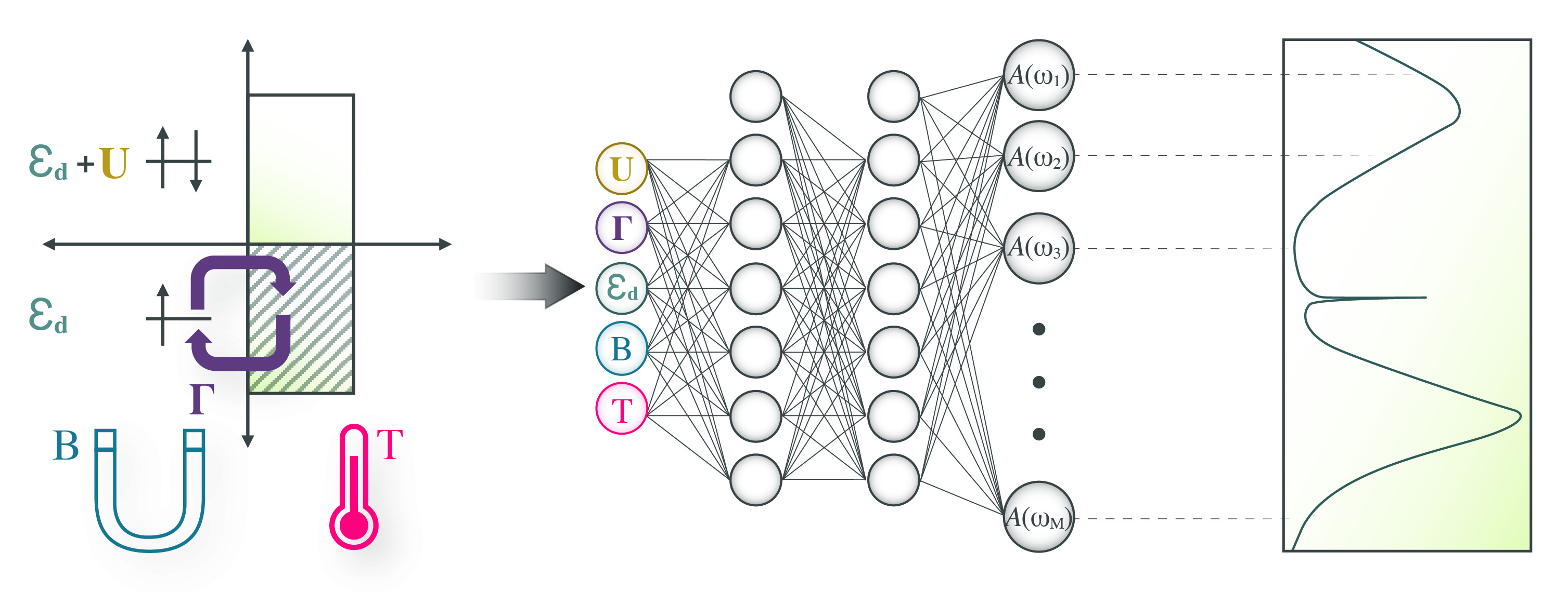
Figure 1: Cartoon of a typical Anderson impurity model with a set of physical input parameters (left). The physical properties are fed as training data into a neural network (center), which then learns to predict the spectral function (right).

DMFT is a Green’s function method Kent and Kotliar (2018) that sums over an infinite set of Feynman diagrams consistent with the self-energy of the single-particle Green’s function being local. In practice, performing this infinite summation amounts to solving a self-consistent quantum impurity problem. Besides lying at the heart of DMFT, quantum impurity problems are interesting many-body systems in and of themselves. They also describe magnetic impurities in metallic systems de Haas et al. (1934); Costi et al. (2009), engineered quantum dots in bosonic or fermionic environments Leggett et al. (1987); Cronenwett et al. (1998); Latta et al. (2011), and boundary edge modes in topologically non-trivial systems Drozdov et al. (2014). They also generically experience low-energy dynamically generated phenomena that are beyond perturbation theory such as the Kondo effect Anderson (1970); Kondo (1964) and the attendant Abrikosov-Suhl resonance that appears at low temperatures and frequencies in the quantum impurity’s spectral response function.

Different techniques are available to find the spectral function of a quantum impurity problem. Included among those that are numerically exact are continuous-time quantum Monte Carlo simulations Gull et al. (2011); Aoki et al. (2014), the numerical renormalization group (NRG) Wilson (1975), and the density matrix renormalization group White (1992). The number of channels in the impurity problem determines the complexity of computing the spectral function (in the context of DMFT, the number of channels in the effective impurity model matches the number of bands involved in the underlying material). Single channel impurity models are relatively cheap to solve numerically while multiple channel impurity problems are exponentially more challenging. For example, five band f-electron materials have associated impurity models requiring petascale computational resources to accurately solve Melnick et al. (2020). Furthermore, DMFT embeds quantum impurity model solutions in a self-consistent loop, requiring multiple solutions for final convergence.

In this light, we ask if machine learning (ML) approaches offer an alternative to expensive many-body simulations of impurity response functions. This question was first posed in Ref. Arsenault et al., 2014, where kernel ridge regression (KRR) models were trained on a small database of about 5000 spectral functions computed at imaginary frequencies. A focus of this study was to understand the optimal parameterization of the spectral function for training purposes, finding that a representation in terms of Legendre polynomials worked best. More recently Ref. Walker et al., 2020 used a set of neural networks to train a spectral solver for a quantum impurity connected to a bath of six sites, and each network was trained to predict the spectral function at a single frequency.

In the work presented herein, we investigate whether an individual model, whether it be KRR or a neural network, can predict the impurity response function in regimes where the relevant energy scales are separated by orders of magnitude and where temperature and magnetic field are also parameters. To this end, we have constructed large ($\sim 10^{5}$) databases of high fidelity spectral functions in the thermodynamic limit using NRG. We examine the dependence of these results on the training set size, as generating large training sets for the multi-channel impurity problems, the problem of ultimate interest, is much more computationally intensive. We use NRG to create our databases as it is an approach that (i) can reliably reach arbitrary, exponentially small dynamically generated energy scales; (ii) computes spectral properties directly on the real frequency axis, and (iii) can work with arbitrary temperatures in an efficient, systematic manner Bulla et al. (2008); Anders and Schiller (2005); Weichselbaum and von Delft (2007); Stadler et al. (2015); Lee et al. (2017). To the best of our knowledge, such high quality NRG databases do not exist for the AIM model.

Quantum Impurity Model. In this work we consider the most elementary of quantum impurity models, the single impurity Anderson model (SIAM) Anderson (1961) with a fixed hybridization function. While we aspire to use ML algorithms Rigo and Mitchell (2020); Hendry and Feiguin (2019) to study multi-channel impurity problems, we begin here with the simpler SIAM test environment. The SIAM Hamiltonian is given by:

$$\hat{H}=\hat{H}_{\mathrm{imp}}+\sum_{\sigma}\int d\varepsilon\,\sqrt{\tfrac{\Gamma(\varepsilon)}{\pi}}(\hat{d}_{\sigma}^{\dagger}\hat{c}_{\varepsilon\sigma}+\mathrm{H.c.})+\int d\varepsilon\,\varepsilon\,\hat{c}_{\varepsilon\sigma}^{\dagger}\hat{c}_{\varepsilon\sigma}.$$ (1)

Here, $\hat{H}_{\mathrm{imp}}=\varepsilon_{d\sigma}\hat{n}_{d\sigma}+U\hat{n}_{d\uparrow}\hat{n}_{d\downarrow}$, where $\hat{d}_{\sigma}^{\dagger}$ creates a particle with spin $\sigma\in\{\uparrow,\downarrow\}$ at the impurity $d$-level at energy $\varepsilon_{d\sigma}=\varepsilon_{d}-\tfrac{\sigma}{2}B$ with $B$ an external magnetic field representing the Zeeman splitting. Double occupation of the impurity levels pays a Coulombic energy penalty, $U,$ as measured by $U\hat{n}_{d\uparrow}\hat{n}_{d\downarrow}$. The coupling of the bath of electrons, $\hat{c}_{\varepsilon\sigma}^{(\dagger)},$ to the impurity is described by the hybridization function, $\Gamma(\varepsilon)=\pi\rho_{\varepsilon}V_{\varepsilon}^{2},$ with $\rho_{\varepsilon}$ the density of states, and $V_{\varepsilon}$ the corresponding hopping matrix element at $\varepsilon$. For simplicity in this work we use a featureless hybridization function, $\Gamma(\varepsilon)=\vartheta(D-|\varepsilon|)\,\Gamma,$ with constant strength $\Gamma=1$ for $|\varepsilon|<D$ and zero elsewhere (we take all energies in units of the half-bandwidth $D=1$, unless specified otherwise, as well as $\hbar=k_{B}=1$).

Database Construction. Inspired by earlier work Arsenault et al. (2014), we started with impurity parameters, U, $\Gamma$, and $\varepsilon_{\mathrm{d}}$, which we expanded to include external parameters $B$ and temperature $T$. For a single data point, these inputs will henceforth be written as the ordered set $x_{p}\equiv\left(U,\Gamma,\varepsilon_{\mathrm{d}},B,T\right)_{p}.$ We randomly select values for the parameters within predefined physically motivated domains. $x_{p}$ is mapped onto the scaled target $y_{p}(\omega)\equiv\pi\Gamma_{p}A_{p}(\omega)\in[0,1]$, where $A(\omega)$ is the corresponding spectral function which we compute via the NRG. Two disjoint sets were generated: the “Anderson" ($\mathcal{D}^{\mathrm{A}}$) and “Kondo" ($\mathcal{D}^{\mathrm{K}}$) sets of sizes $|\mathcal{D}^{\mathrm{A}}|\approx 600\mathrm{k}$ and $|\mathcal{D}^{\mathrm{K}}|\approx 410\mathrm{k}.$ Both sets produce related physics and span similar regions of the 5D input hyperspace (see Fig. 2). As the ML results are similar, we present the Anderson Set results unless otherwise specified. Details on the input parameter generation including histograms and results on the Kondo Set can be found in the Appendices SM .

In practice, spectra were examined between $\omega=\pm 0.8$ to circumvent band edge artifacts, and within that window the spectra are sampled on a refined mixed linear-logarithmic frequency grid $\omega_{i}$ for $i=1,\ldots,M$ with $M=333$. Finally, all regions of the input hyperspace were sufficiently represented according to the trials’ smallest physical energy (SPE) scale, defined as $E_{0}\equiv\max(T,T_{\mathrm{K}},|B|),$ where $T_{\mathrm{K}}$ is the Kondo temperature SM .

Each dataset contains data points $(x_{p},y_{p})$, and is partitioned into disjoint training $(\mathcal{R}^{\Omega})$, cross-validation $(\mathcal{V}^{\Omega})$, and testing $(\mathcal{T}^{\Omega})$ sets, with $\Omega\in\{\mathrm{A},\mathrm{K}\}$ for the Anderson and Kondo datasets, respectively. We use approximately 2% of the data for cross-validation, another 2% for testing, and the rest for training . In an effort to evaluate how the data selection method of the minimal training sets affects the results, we also define two subsets of $\mathcal{R},$ both of size 50k. The first is a randomly down-sampled subset $\mathcal{R}_{\mathrm{r}}\subset\mathcal{R}.$ The second is a furthest-points down-sampled (FPS) subset $\mathcal{R}_{\mathrm{f}}\subset\mathcal{R}$ constructed by first selecting a random point, and then iteratively sampling the next furthest point in the remainder of the scaled, 5D parameter-space. Models are hyper parameter-tuned using the validation set, and all results presented in this work correspond to the testing sets, both of which are consistent regardless of the model or training set.

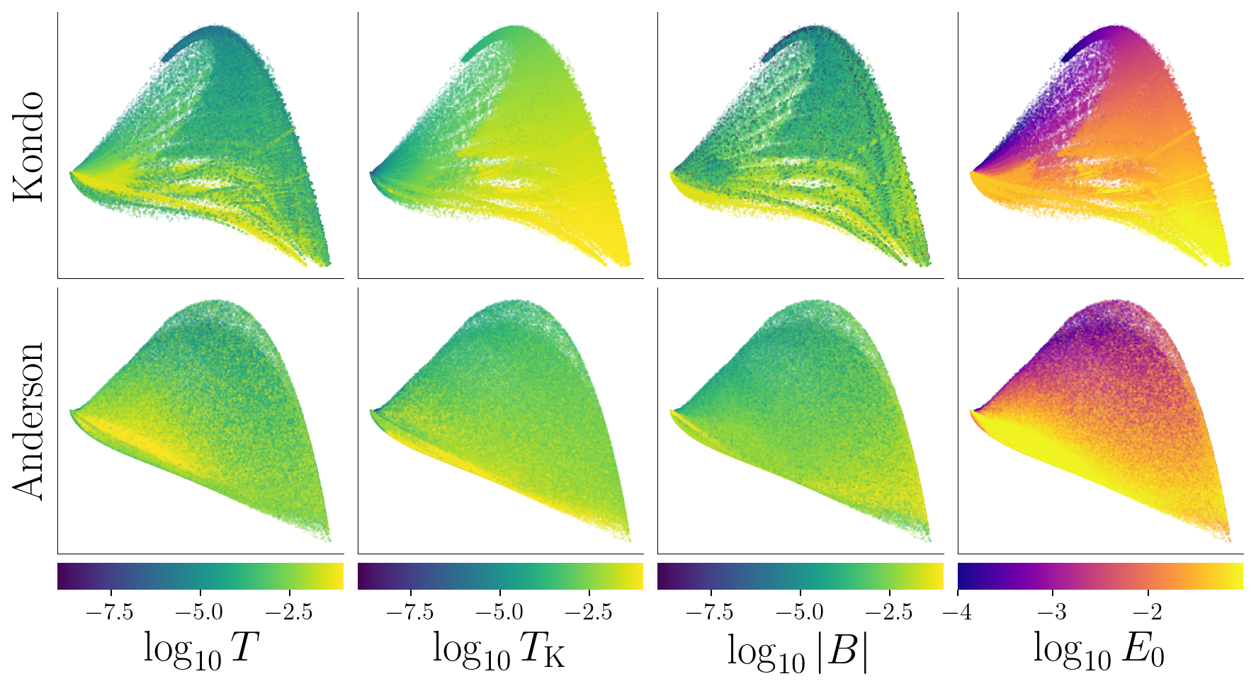
Figure 2: Principal component analysis performed on the Kondo (top) and Anderson (bottom) spectral datasets. In each of the four columns the same PCA data are colored in terms of different parameters, left to right: temperature, Kondo temperature, magnetic field strength, and $E_{0}$.

In order to visually evaluate the integrity of the generated datasets, we performed a principal component analysis (PCA) in the spectral space, reducing the dimension of each spectrum from $M$ to $2$. The results are plotted in Fig. 2, and color-coded with respect to parameters of the SIAM that are most directly relevant for the physical low-energy regime, $T$, $T_{\mathrm{K}}$, $|B|$, and the derived $E_{0}$. Overall, the smooth color gradients observed in the PCA plots suggest that the physically-relevant input parameters can be mapped continuously to prominent spectral features. Additionally, one can identify interesting trends within the physical parameter regimes. In the plots involving $E_{0}$, the lowest values cluster at the top and towards the left, while the largest $E_{0}$ scales concentrate at the bottom towards the right/left for the Kondo/Anderson dataset. This suggests that the dynamically generated Kondo peak at low energies and the higher energy side peaks correspond to different spectral features, as already understood from domain knowledge. Despite the overall similarity between the Kondo and Anderson PCA plots, there are subtle differences. For example, in the Kondo set, the input parameters were generated on a grid SM leading to streaks in the PCA plots while such streaks are absent in the uniformly sampled Anderson set. These PCA plots qualitatively confirm the physical intuition that a well-defined mapping exists between the input parameters, which determine the physics of the system, and the spectral functions. This suggests that machine learning algorithms are well suited to modeling the feature-target mapping.

Model Results & Discussion. We use the mean absolute error (MAE) to characterize model performance. The MAE between a ground truth NRG spectrum $y_{p}(\omega)$ and ML-predicted $\hat{y}_{p}(\omega)$ is defined as an average over the testing set,

$$\delta y_{p}=\frac{1}{M}\sum_{i=1}^{M}|y_{p}(\omega_{i})-\hat{y}_{p}(\omega_{i})|,\quad\overline{\delta y}=\frac{1}{|\mathcal{T}|}\sum_{y_{p}\in\mathcal{T}}\delta y_{p},$$ (2)

as displayed in Table 1.

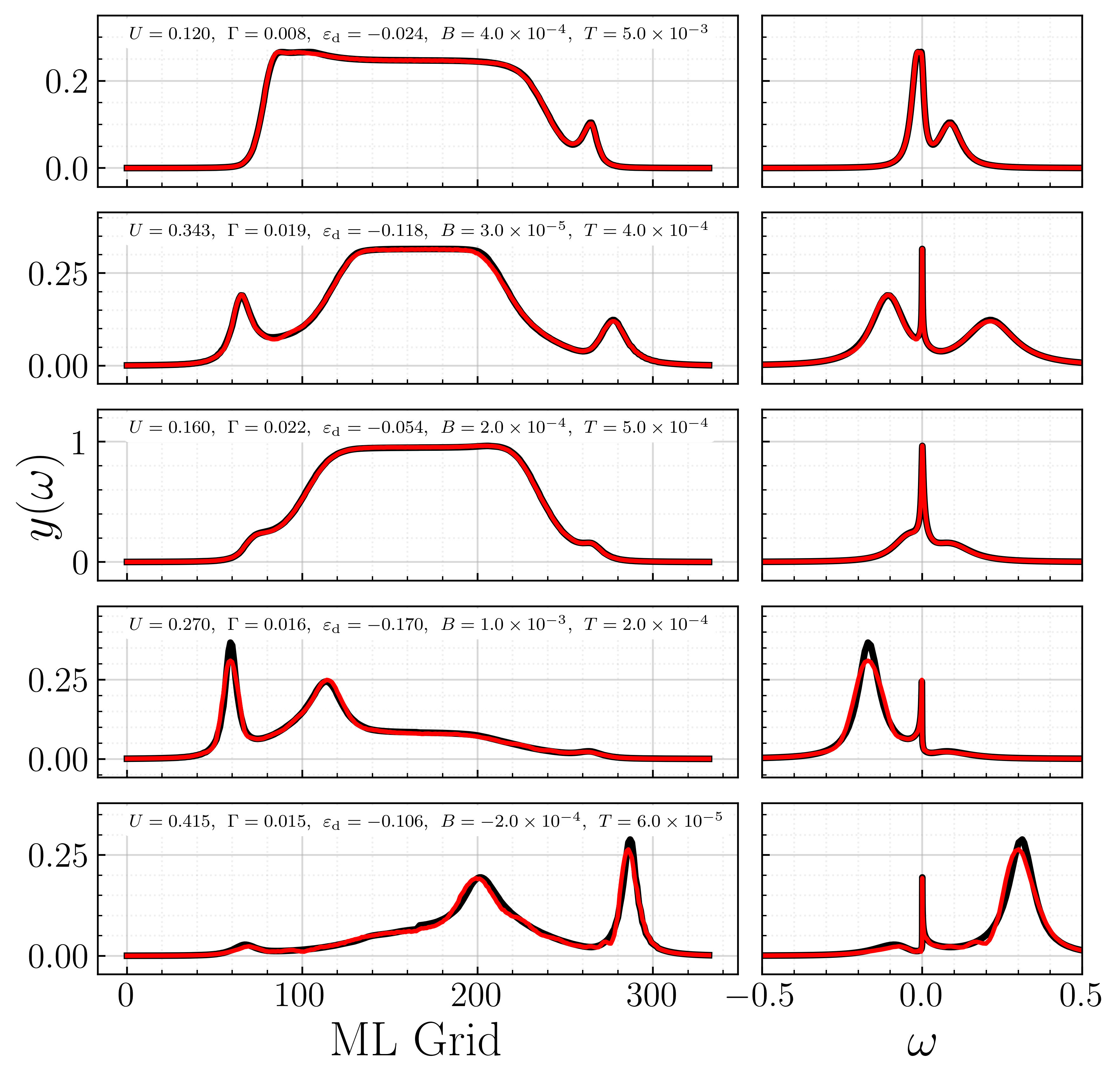
Figure 3: Representative ground truth (black) and MLP-predicted (red) spectral functions from the testing set, $\mathcal{T}^{\mathrm{A}},$ from the model trained on $\mathcal{R}^{\mathrm{A}}.$ Data correspond to the best example of each of the five pentiles of the data top to bottom, respectively. The system parameters $x_{p}\equiv\left(U,\Gamma,\varepsilon_{\mathrm{d}},B,T\right)_{p}$ are specified within each panel. As the algorithms have no notion of the $\omega$-grid on which the spectra are defined, we present the “ML-grid" (left) which represents the spectral functions, $y_{p}=\pi\Gamma_{p}A_{p}$, on a uniformly-spaced grid (emphasizing how the algorithms “see" the targets).

Table 1: Summary of average and standard deviations of mean absolute error [cf. Eq. (2)] of all trained models as computed on test sets, $\mathcal{T}^{\Omega}$. The training sets used are shown in parenthesis, e.g., MLP$(\mathcal{R}_{\mathrm{f}})$ indicates the MLP trained on the down-sampled 50k trial $\mathcal{R}_{\mathrm{f}}$ sets but still evaluated on the appropriate $\mathcal{T}$. All KRR$(\mathcal{R}_{\mathrm{r}})$ training attempts yielded poor predictions with $r^{2}<0$. DC-KRR$(\mathcal{R}_{\mathrm{F}})$ trained on the full training set $\mathcal{R}$ but in sequentially-sampled subsets ordered by the FPS algorithm as explained in Eq. (3).

$\Omega$	Baseline	MLP$(\mathcal{R})$	MLP$(\mathcal{R}_{\mathrm{r}})$	MLP$(\mathcal{R}_{\mathrm{f}})$	KRR$(\mathcal{R}_{\mathrm{r}})$	KRR$(\mathcal{R}_{\mathrm{f}})$	DC-KRR$(\mathcal{R}_{\mathrm{F}})$
A	$0.126\pm 0.054$	$0.003\pm 0.003$	$0.091\pm 0.070$	$0.014\pm 0.013$	$0.084\pm 0.068$	$0.021\pm 0.023$	$0.017\pm 0.026$
K	$0.234\pm 0.076$	$0.003\pm 0.002$	$0.152\pm 0.141$	$0.010\pm 0.009$	$0.152\pm 0.145$	$0.019\pm 0.021$	$0.035\pm 0.033$

We introduce a measure of the spectral data variation, referred to as the baseline error, as the MAE of the test set against its average spectrum, $\overline{y}(\omega)\equiv\frac{1}{|\mathcal{T}|}\sum_{y_{p}\in\mathcal{T}}y_{p}(\omega)$. In a dataset with a high degree of variance, such as $\mathcal{R}^{\mathrm{A}}$ or $\mathcal{R}^{\mathrm{K}}$, we expect the baseline error to be quite large; our goal is to train a machine learning model to learn the mapping between the input and output effectively, and thus significantly outperform this baseline. We begin our investigation with a multi-layer perceptron (MLP), a deep learning model capable of capturing highly non-linear relations in high-dimensional data. We observe a superb performance from the MLP trained on $\mathcal{R}$, where the results outperform the baseline by factors of roughly 40 and 80 on the Anderson ($\overline{\delta y}=0.003$) and Kondo ($\overline{\delta y}=0.003$) testing sets, respectively.

From each pentile of the Anderson test set, the best representative examples of the model predictions are presented in Fig. 3. We first note that all important spectral features are well-reproduced in these examples including the peak heights, widths, and locations of the sharp central peak and the broader side peaks. As expected, models trained using all of $\mathcal{R}$ present the best results. However, models trained using the FPS subset, $\mathcal{R}_{\mathrm{f}}$, which only constitutes about 10% of each of the full training sets, also perform surprisingly well, indicating that even a moderately sized training set can result in accurate predictions, if the sampling of the input-parameter space is well-spanned. This is critically important for more complex physical problems where generating training data becomes much more expensive. By comparison, models trained on a randomly sampled subset, $\mathcal{R}_{\mathrm{r}},$ of the same size performs roughly an order of magnitude worse than $\mathcal{R}_{\mathrm{f}}$, and even barely outperforms the baseline.

We also examine analytical results from the KRR model Pedregosa et al. (2011); Zhang et al. (2013). However, this method scales cubically with training set size $|\mathcal{R}_{x}|$ with $x\in\{\mathrm{r},\mathrm{f}\},$ as it requires a full matrix inversion, making it intractable to use the full $\mathcal{R}$ at once. We mitigate this problem in two ways: using down-sampled training sets of $\mathcal{R}_{\mathrm{r}}$ or $\mathcal{R}_{\mathrm{f}}$, and a divide-and-conquer KRR (DC-KRR) algorithm Zhang et al. (2013); You et al. (2018). Details regarding KRR and DC-KRR algorithms and hyperparameters can be found in SM . Models trained using $\mathcal{R}_{\mathrm{f}}$ perform an order of magnitude better, and have higher coefficients of determination $(r^{2})$ than the $\mathcal{R}_{\mathrm{r}}$ counterparts, in agreement with our earlier findings for the MLP.

The final KRR models trained on $\mathcal{R}_{\mathrm{f}}$ are superior to the baseline error by factors of roughly 6 and 10 for the Anderson and Kondo sets, respectively. Interestingly, both the MLP and KRR models trained with the down-sampled $\mathcal{R}_{\mathrm{r}}$ achieved nearly identical results, and both are essentially indistinguishable from the baselines, indicating there is insufficient information contained in the randomly-downsampled training sets to train successful models.

In contrast, DC-KRR uses the full data set by partitioning $\mathcal{R}$ into $S$ consecutive (ordered), disjoint subsets $\mathcal{R}_{\mathrm{f}}^{(s)}$, such that

$$\mathcal{R}_{\mathrm{F}}=\left(\mathcal{R}_{\mathrm{f}}^{(1)},\mathcal{R}_{\mathrm{f}}^{(2)},...,\mathcal{R}_{\mathrm{f}}^{(S)}\right),\quad|\mathcal{R}_{\mathrm{f}}^{(s)}|\approx 50\mathrm{k},$$ (3)

where the union $\bigcup_{s}\mathcal{R}_{\mathrm{f}}^{(s)}$ is equivalent to the full training set $\mathcal{R}$ with respect to the earlier analysis, and it holds that $\mathcal{R}_{\mathrm{f}}\equiv\mathcal{R}_{\mathrm{f}}^{(1)}.$ We then train an independent KRR model for each $\mathcal{R}_{\mathrm{f}}^{(s)}$ and average the resulting learned parameters. Because the KRR models performed poorly with $\mathcal{R}_{\mathrm{r}}$ we only present the DC-KRR whose subsets were indexed according to the FPS algorithm in Table 1. Here, both models exceed the baseline average by a factor of roughly 7. Despite training on the full data set, the DC-KRR performs comparably to the KRR($\mathcal{R}_{\mathrm{f}}$) model.

Conclusion. In summary we have shown that ML algorithms can predict state-of-the-art Anderson impurity model spectra to overall quantitative accuracy at a speedup of $10^{5}$ over NRG. We have found that the use of furthest points sampling can significantly reduce the required amount of training data to achieve satisfactory accuracy. While KRR and DC-KRR are effective for small datasets or large datasets properly divided into chunks of small datasets, our results imply that deep learning algorithms trained on sufficient amount of data are superior for predicting both the single and many-body features of a SIAM spectral function. Future work will expand the physical model to include additional impurity parameters, most importantly a structured hybridization function and more channels, and thus examine the viability of a ML algorithm in the context of a DMFT self-consistent loop.

A0 A1: Dataset construction

We use the Numerical Renormalization Group (NRG, Wilson (1975); Bulla et al. (2008)) to compute the impurity spectral functions. The NRG obtains the spectral data directly on the real-frequency axis for arbitrary temperatures where we use the fdm-NRG approach Weichselbaum and von Delft (2007). We use a typical discretization parameter of $\Lambda=2$, with the discrete data subsequently smoothened using standard log-Gaussian broadening schemes. We also compute the local self-energy $\Sigma^{\mathrm{imp}}(\omega)$ to improve spectral resolution of the NRG data Bulla et al. (1998).

Each NRG trial takes a set of randomly sampled system parameters $x_{p}\equiv\left(U,\Gamma,\varepsilon_{\mathrm{d}},B,T\right)_{p}$, and generates a spectral function $\pi\Gamma A(\omega)$. Here the factor of $\pi\Gamma$ maintains normalization, such that, e.g., $\pi\Gamma A(0)\leq 1$ can be interpreted as transmission probability in transport measurements. Meir et al. (1991); Goldhaber-Gordon et al. (1998); Costi et al. (2009) The hybridization strength $\Gamma$ is derived from the hybridization function chosen to be featureless, i.e. $\Gamma(\omega)=\Gamma\vartheta(D-|\omega|)$, Wilson (1975); Bulla et al. (2008) where the half-bandwidth $D:=1$ sets the unit of energy throughout, unless specified otherwise.

Due to the artificial sharp cutoff at the band edge caused by our choice of constant hybridization strength, we only consider the energy window $\omega=[-0.8,0.8]\,D$ to avoid artefacts at the band edge. We do not examine regions, and hence also ignore spectral weight beyond the band edge. Within the specified window, we coarse-grain the essentially continuous NRG data to the same fixed frequency grid to be used in the machine learning (ML) algorithms. This grid is chosen such that it is linearly spaced for larger frequencies (67 points for $\omega\in\left[0.1,0.8\right]$), and logarithmically spaced for smaller frequencies (99 points for $\omega\in[10^{-5},10^{-1}]$). The same grid is mirrored for negative frequencies. With the addition of a single point at $\omega=0$ to bridge the logarithmic grid from positive to negative we have our final 333 coarse-grain frequency points. The grid $\omega_{i}$ is the same for every trial, which thus maps the five physical parameters to the normalized spectral function,

$$x_{p}\quad\mapsto\quad y_{p,i}\equiv\pi\Gamma_{p}\,A_{p}(\omega_{i}).$$ (AA0.1)

The five physical parameters $x_{p}$ are referred to as the input features, and the 333 $y_{p}$ values as the output targets in our ML algorithms.

The smallest non-zero $\omega$ value in our logarithmic frequency grid is $10^{-5}$, which is well above the NRG’s minimum set at $\sim 10^{-6}$ as determined by our Wilson chain length of $L=50$ and discretization parameter $\Lambda=2$. Therefore, to ensure that features are captured within our frequency grid for ML, any NRG trials with smallest physical energy (SPE) $E_{0}$ scales smaller than $10^{-4}$ are removed. The SPE scale of each trial is defined by:

$$E_{0}=\mathrm{max}\left(|B|,T,T_{K}\right)\text{ ,}$$ (AA0.2)

with the Kondo temperature $T_{K}$ determined according to Haldane’s formula Haldane (1978),

$$T_{K}=\min\bigl{(}0.575,\sqrt{\tfrac{U\Gamma}{2}}\bigr{)}\exp\bigl{(}\tfrac{\pi\varepsilon_{d}(\varepsilon_{d}+U)}{2U\Gamma}\bigr{)}\text{ .}$$ (AA0.3)

By definition of being the smallest physical energy scale, all physical features in the spectral data are at least as broad as the SPE. For example, low-energy Kondo features (described by $T_{K}$ which is defined at $B=T=0$) are physically smeared out at the energy scale of $\lvert B\rvert$ or $T$ if these are larger than $T_{K}$.

A1.A1.1  A1.1: Physical Parameter Selection

The five physical parameters for the single impurity Anderson model (SIAM) in this work are collected as an ordered set $x_{p}\equiv\left(U,\Gamma,\varepsilon_{d},B,T\right)_{p}$. Inspired by the earlier work of Arsenault et. al. Arsenault et al. (2014), we began with all five parameters sampled on pre-selected grids (referred to as ‘on-grid data’ below). This initial set contained just over 1.45 million trials (see blue bars in Fig. A1). However, we eventually found it favorable to supplement these with 329k additional trials with random parameter values from preset ranges (‘off-grid’) provided that their $E_{0}$ values fell within the targeted range of $[10^{-4},10^{-1}]$ (see green bars in Fig. A1). Ultimately we removed any trials where the $E_{0}$ did not fall in the desired energy range (see right panel in Fig. A1).

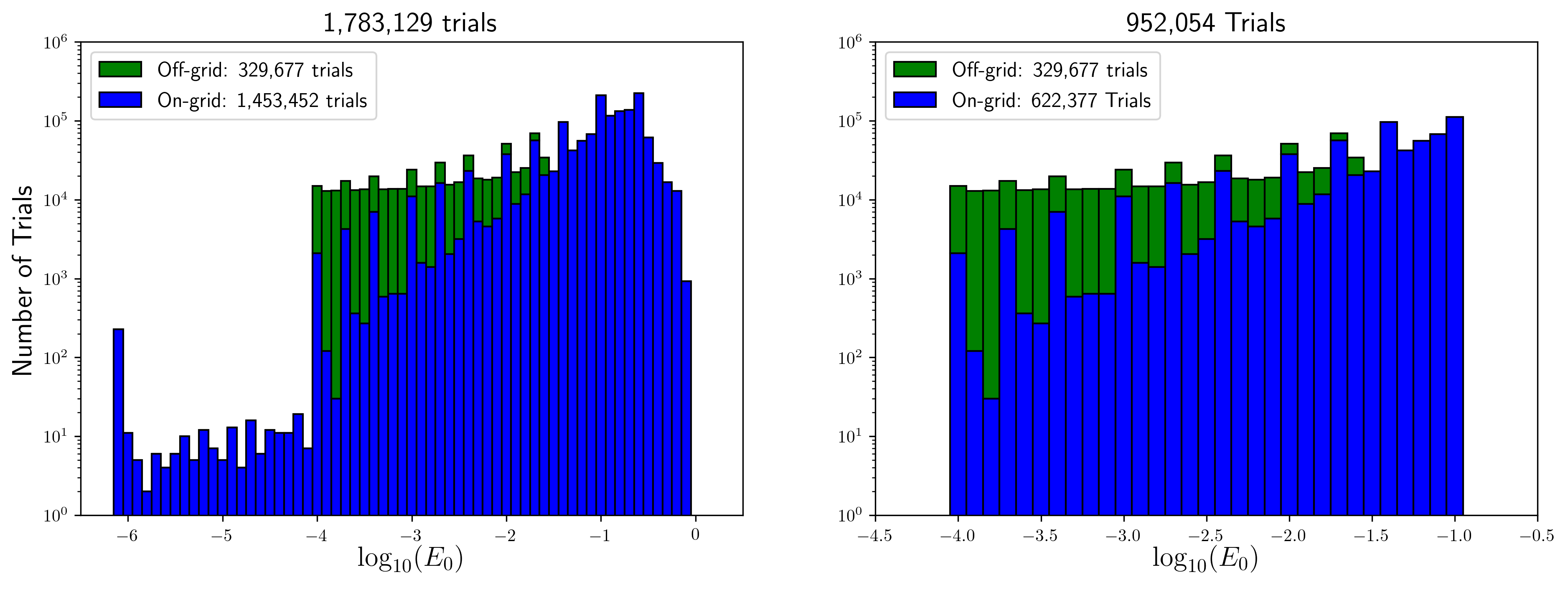
Figure A1: SPE histograms for the Kondo data set. The original on-grid data (blue) of 1.45 million trials was supplemented by an additional 329k off-grid trials (green) to ensure a more even $E_{0}$ distribution on a log-scale (left panel). Trials with SPE values outside our range of interest $E_{0}\in[10^{-4},10^{-1}]$ were discarded, which gave rise to a final SPE distribution (right panel). Bin widths are the same in both panels.

We then enforced the additional requirement on the hybridization strength $\Gamma$,

$$\Gamma>\mathrm{min}\bigl{(}\tfrac{|B|}{5},\tfrac{U}{40}\bigr{)}$$ (AA1.4)

in order to avoid extremely narrow features in the spectral data comparable to or below the frequency grid spacing chosen for ML. From a physical perspective, this would correspond to an essentially decoupled and hence trivial impurity. Finally, a randomly selected subset of trials that satisfied the above requirements were selected for a data set of $\sim$ 411k trials. We refer to this dataset as the “Kondo Set” because many parameter sets have large Coulomb energies $U$ comparable to or larger than the half bandwidth (i.e. $U\gtrsim 1$). The SPE distribution for the Kondo set is presented in Fig. A2, while the parameter value distribution is shown in black in Fig. A5.

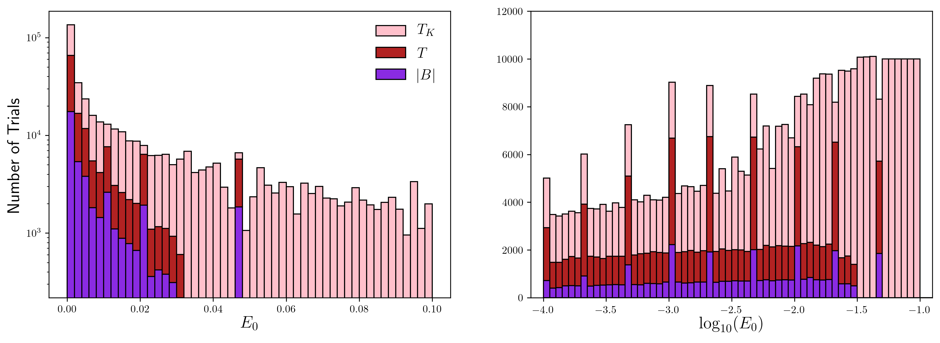
Figure A2: SPE histogram of 411,267 data point Kondo set on linear and log-scale (left and right panel respectively), with approximately equal distribution across trials at lower energies only where $E_{0}$ is dominated by $|B|$, $T$, or $T_{K}$. Regularly spaced spikes in right panel are due to the on-grid portion of the Kondo set.

In contrast, the “Anderson Set” was designed with an even SPE distribution in mind, while also keeping $U<0.5$ right from the start as shown in black in the left-most panels of Fig. A4. To be specific, the parameters for this data set were sampled in the following manner: (i) randomly choose an SPE value with a flat distribution on the log-scale in the range $E_{0}\in[10^{-4},10^{-1}]$ (ii) randomly select which of the three parameters $|B|$, $T$, or $T_{K}$ takes that $E_{0}$ value, then (iii) ensure that the other two parameters are smaller than $E_{0}$, using the range $[0,E_{0}/10]$. Both positive and negative values for $B$ are computed in all cases. With $T_{K}$ fixed, (iv) the remaining values for $U$, $\varepsilon_{d}$, and $\Gamma$ are sampled based on Eq. (AA0.3). Specifically, the values for $\Gamma$ and $U$ are assigned at random on a linear scale below bandwidth, while still ensuring Eq. (AA1.4). This fixes the prefactor in Eq. (AA0.3). By taking the logarithm, we then solve for $\varepsilon_{d}$. If no valid solutions exist for $\varepsilon_{d}$ given the choices in $U$ and $\Gamma$, we go back and repeat step (iv). With this basic algorithm we generated a total of about 600k trials with the desired flat SPE distribution as demonstrated in Fig. A3. The parameter distribution for the Anderson Set is shown in black in Fig. A4.

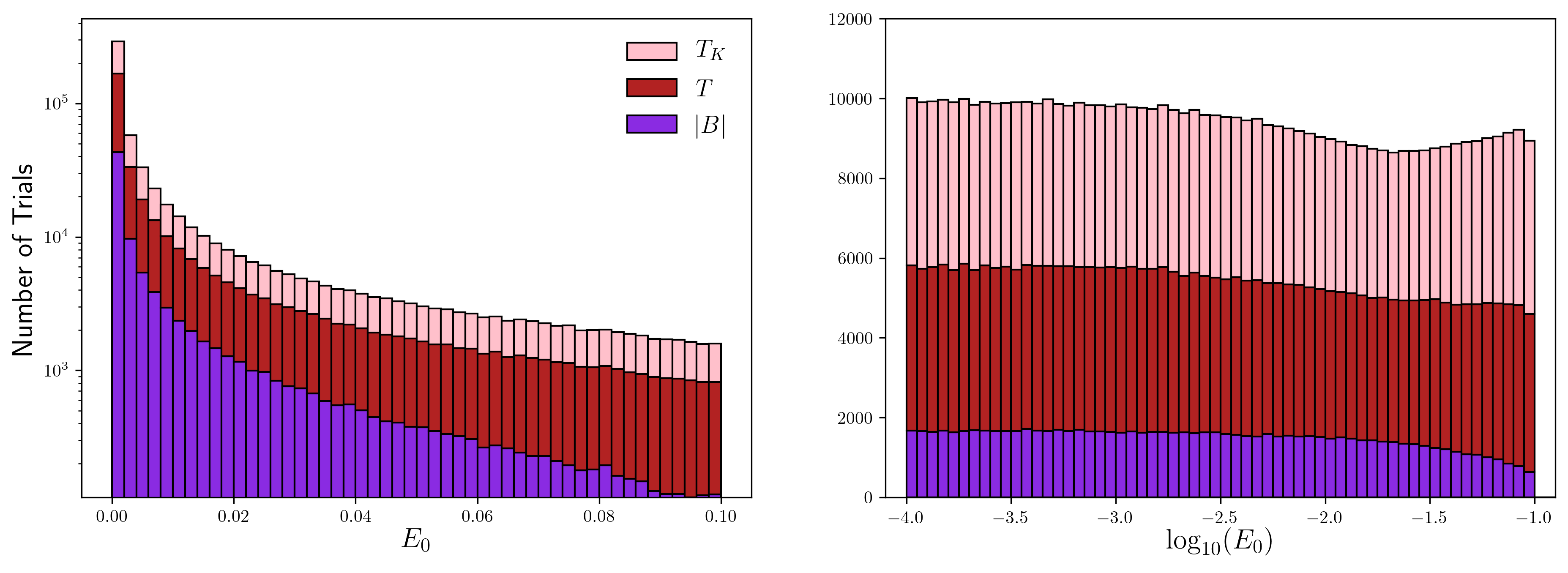
Figure A3: SPE histogram of 599,578 data point Anderson set on linear and log-scale (left and right panel respectively), with approximately equal distribution across trials where $E_{0}$ is dominated by $|B|$, $T$, or $T_{K}$.

A2.A2.2  A1.2: Split selection

The full datasets for the Anderson and Kondo datasets are labeled $\mathcal{D}^{\Omega}$ with $\Omega\in\{\mathrm{A},\mathrm{K}\}.$ Each contain about 500k of data points $(x_{p},y_{p})$ that are split into disjoint training ($\mathcal{R}^{\Omega}$), validation ($\mathcal{V}^{\Omega}$), and testing ($\mathcal{T}^{\Omega}$) sets. Since the Anderson and Kondo sets themselves are disjoint and also mostly dealt with on an equal footing, we generally suppress the subscript $\Omega$ for readability unless stated otherwise. The two pairs of validation and testing sets are fixed for the entirety of this work. The splits were generated as follows:

1. The testing set, $\mathcal{T}^{\Omega},$ contains roughly 2% of the total data and is selected by randomly down-sampling $\mathcal{D}^{\Omega}$. It is evaluated at the end of the pipeline, and represents the most unbiased representation of the model performance. All results are evaluated on the testing set, unless explicitly stated otherwise.

2. The validation set, $\mathcal{V}^{\Omega},$ also contains roughly 2% of the total data, and is also selected by randomly down-sampling $\mathcal{D}^{\Omega}.$ It is used only to tune model hyperparameters.

3. The full training set, $\mathcal{R}$ (with $\Omega$ indexing suppressed), contains 96% of the total data and is used to train the model. The different versions of the training set are explained below.

   • The randomly sampled training set $\mathcal{R}_{\mathrm{r}}$ contains 50k data points. It is selected by randomly down-sampling $\mathcal{R}.$

   • The furthest points-sampled (FPS) training set $\mathcal{R}_{\mathrm{f}}$ contains 50k data points. It is selected via the algorithm presented in Section A1.4.

   • For divide-and-conquer DC-KRR only, we generate a collection of ordered disjoint subsets $\mathcal{R}_{\mathrm{F}}\equiv\left(\mathcal{R}_{\mathrm{f}}^{(1)},\mathcal{R}_{\mathrm{f}}^{(2)},\ldots,\mathcal{R}_{\mathrm{f}}^{(S)}\right)$, where the set itself $\mathcal{R}=\bigcup_{s=1}^{S}\mathcal{R}_{\mathrm{f}}^{(s)}$ (i.e., the unordered union of the subsets are equivalent to the full training set). The sequence is ordered in the sense that the $\mathcal{R}_{\mathrm{f}}^{(s)}$ are generated consecutively using the algorithm presented in Section A1.4. As an example, the sampling of $\mathcal{R}_{\mathrm{f}}^{(s)}$ excludes samples already included in $\{\mathcal{R}_{\mathrm{f}}^{(1)},\ldots,\mathcal{R}_{\mathrm{f}}^{(s-1)}\},$ and the first point in $\mathcal{R}_{\mathrm{f}}^{(s)}$ is furthest-sampled from the last point in $\mathcal{R}_{\mathrm{f}}^{(s-1)}.$ Note also that $\mathcal{R}_{\mathrm{f}}^{(1)}=\mathcal{R}_{\mathrm{f}}.$

A3.A3.3  A1.3: Preprocessing input features (symlog scaling)

Anderson and Kondo-type models frequently exhibit dynamically generated, exponentially small energy scales. Hence the parameters that enter the SPE in Eq. AA0.2, namely $T_{\mathrm{K}}$, $B$, and $T$, were sampled on a logarithmic scale that stretches over several orders of magnitude. Therefore, prior to model training, one is naturally led to also apply a (symmetric) logarithmic (“symlog”) rescaling to the input features $x_{p}$. Feature scaling was necessary for the MLP and the analytical methods when $\mathcal{R}_{\mathrm{R}}$ was used, as described elsewhere in this document.

Given that the value for $T_{\mathrm{K}}$ itself is not a bare Hamiltonian parameter, we apply the following logarithmic scaling to $\Gamma$, $B$, and $T$:

$$\Gamma \to \log_{10}\,\Gamma$$

$$B \to \mathrm{symlog}_{10}(B)\equiv\mathrm{sgn}(B)\log_{10}|B|$$ (AA3.5)

$$T \to \log_{10}\,T\text{ ,}$$

where $U$ and $\varepsilon_{d}$ are left on the linear scale. Here $\Gamma,T>0$ are always chosen non-zero, yet possibly exponentially small. Also, we always have $|B|<1$, and in the case that $B=0$, the trial’s $B$ value is reset to an order of magnitude smaller than the smallest non-negative $B$ value in the set.

After performing the scaling step in Eq. A3.A3.3, the mean ($\mu$) and standard deviation ($\sigma$) are computed for each of the 5 components $x_{p}^{(i)}\in x_{p}$ in the current training set. Then we use $x_{p}^{(i)}\rightarrow\frac{x_{p}^{(i)}-\mu^{(i)}}{\sigma^{(i)}}$ for every trial from the training, validation, and testing sets.

A4.A4.4  A1.4: Furthest points sampling algorithm

Here we employ a relatively simple algorithm for sampling data points in an arbitrary dimensional space. Note that sampling is performed on scaled features as to treat their notion of distance on equal footing. The algorithm is defined below:

1. Select a random point $x_{p}\in\mathcal{R}$ (here, $x_{p}$ represents the 5-dimensional input parameter vector, i.e., the feature space). It is labeled the current point, and added as first point to the set of sampled points $\mathcal{R}_{\mathrm{F}}$.

2. Find the point that is furthest away from the current point that has not yet been selected, and add it to the set of sampled points. We define distance by $||\cdot||_{L_{d}}$ with $d=2$.

3. Repeat step 2 until the desired size of $\mathcal{R}_{\mathrm{F}}$ is reached.

A5.A5.5  A1.5: Parameter Distributions

In this section we present the input feature distributions. In Fig. A4 we show the full Anderson set with its two down-sampled subsets which were plotted with a degree of translucency to exhibit the concentration of the down-sampled trials. One can immediately observe that the furthest point sampled data is more diffuse whereas the random points tend to concentrate in several regions in each distribution. In Fig. A5 we present the same data for the full Kondo set. Here, we can clearly see the striations due to the ‘on-grid’ trials as opposed to the clusters of “off-grid" trials explained in Section A1.

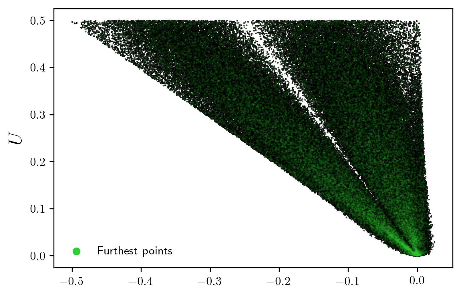
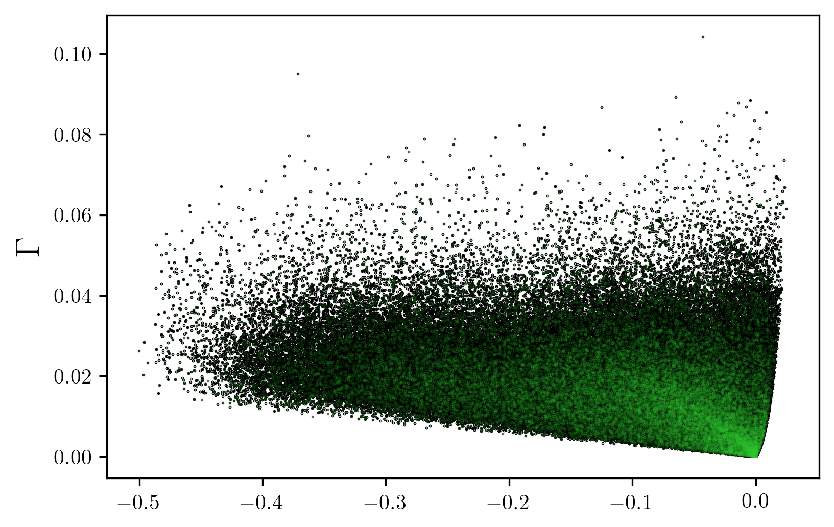
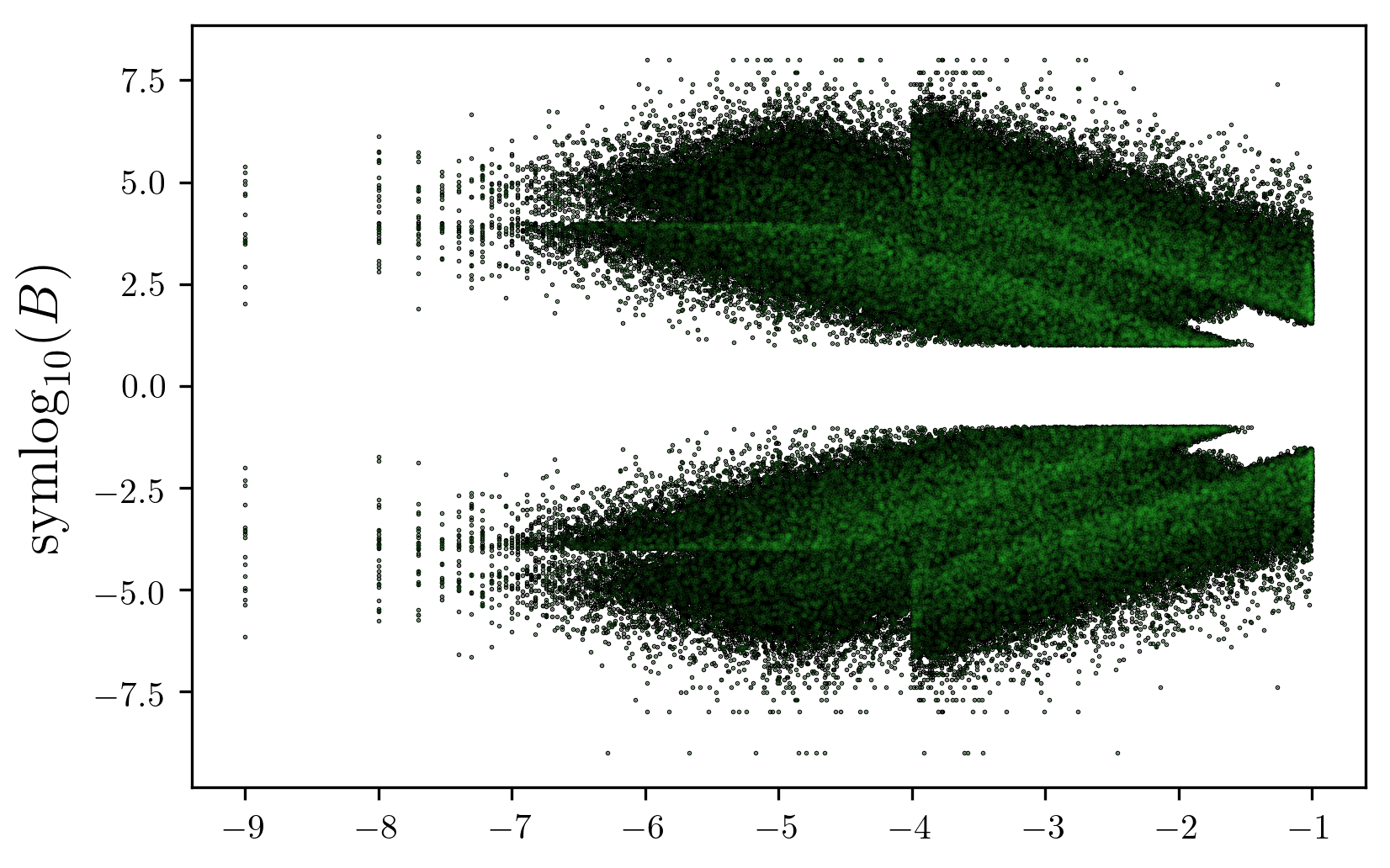
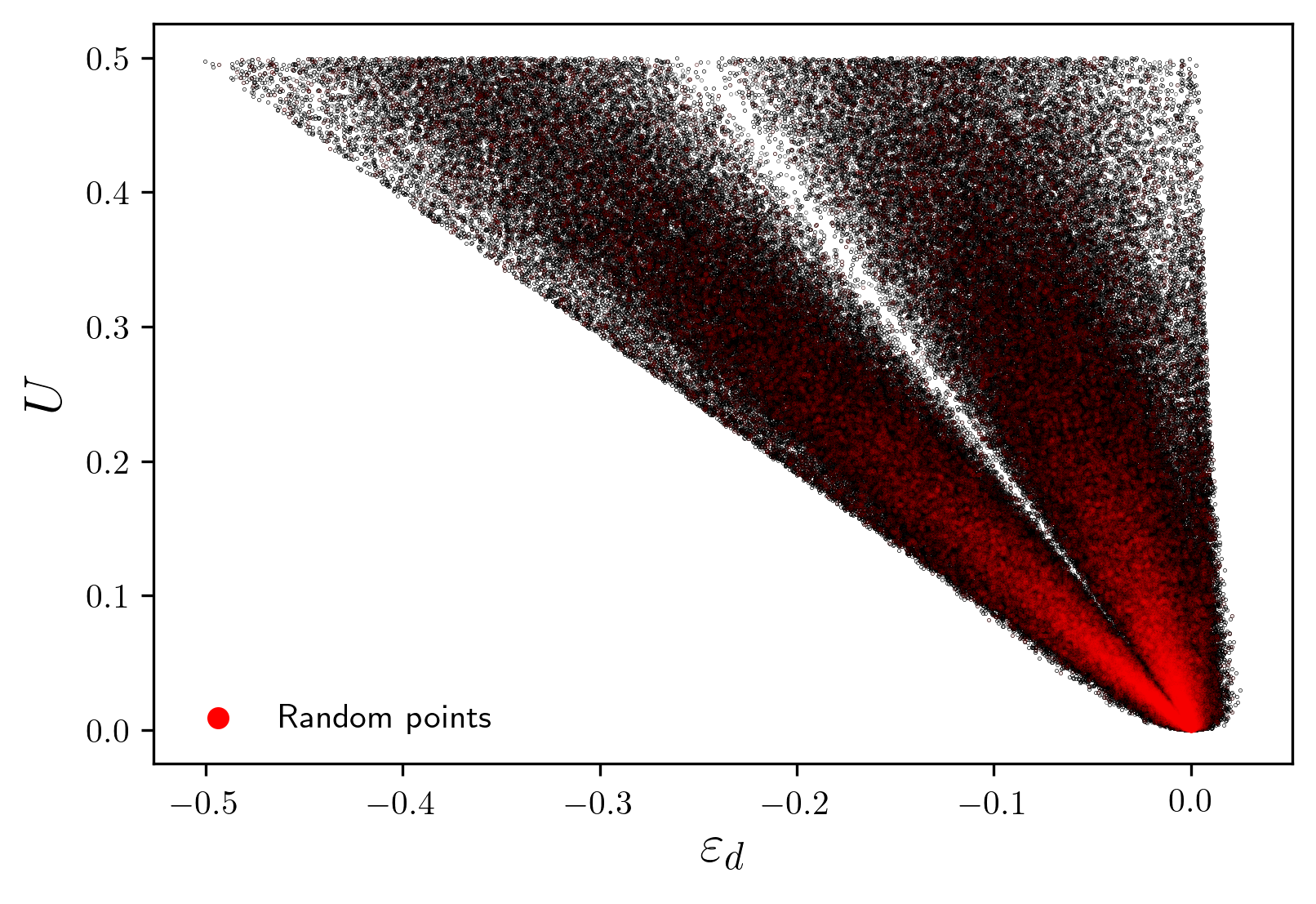
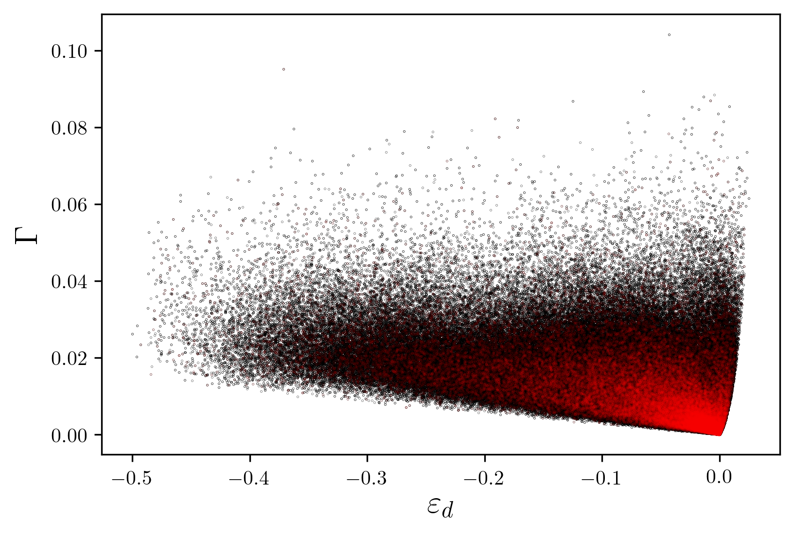
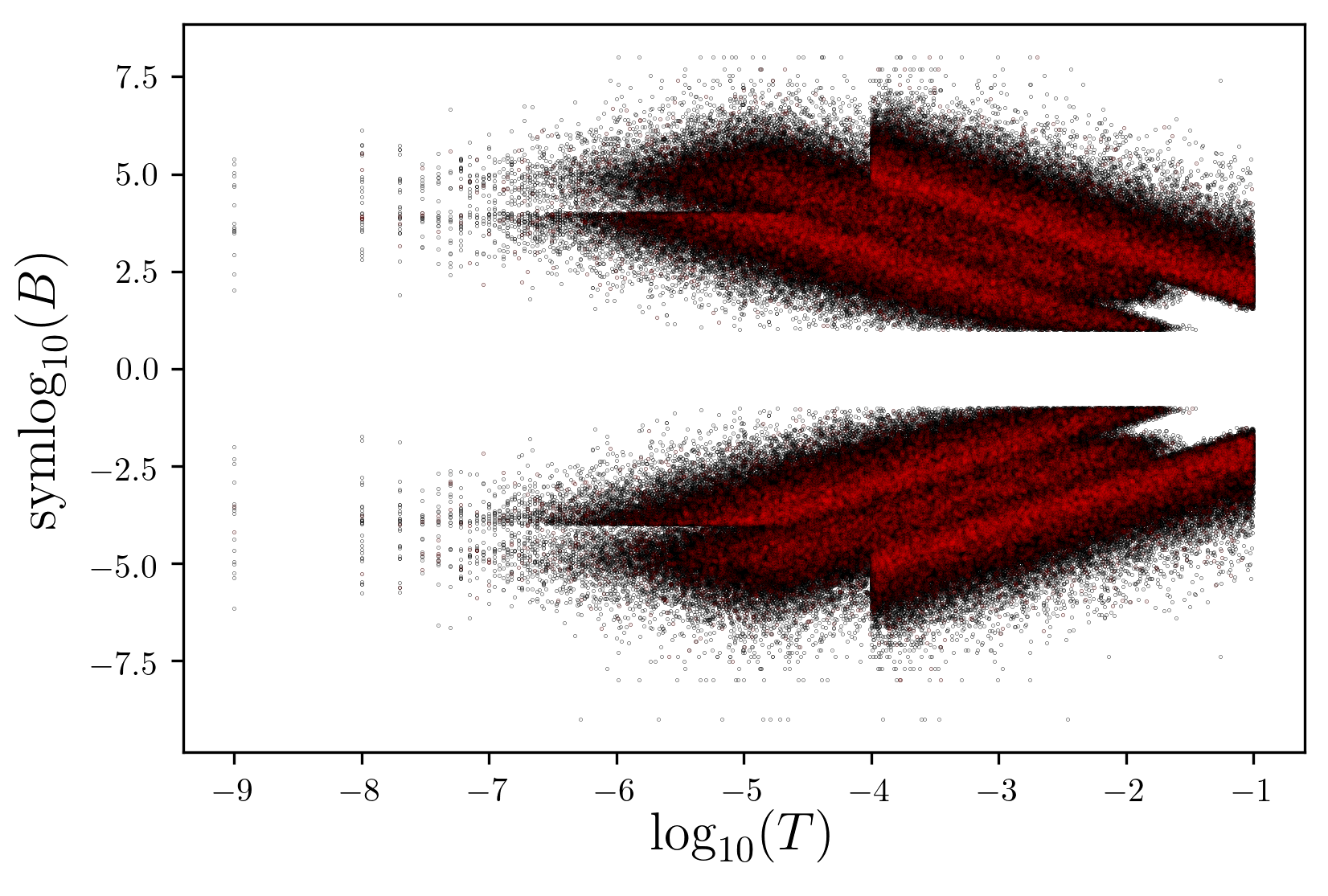
Figure A4: The input feature distribution for the full Anderson set is presented in black. Elements from the down-sampled subsets of the furthest point and random point algorithms each representing approximately 10% of the full set are superimposed in color at 10% opacity to exhibit trial density. The top row shows the furthest point distribution in green while the bottom row shows the random points in red. See Sections A1.3 and A1.4 for additional information regarding the symmetric logarithm (symlog₁₀) procedure and furthest-point sampling algorithm respectively.

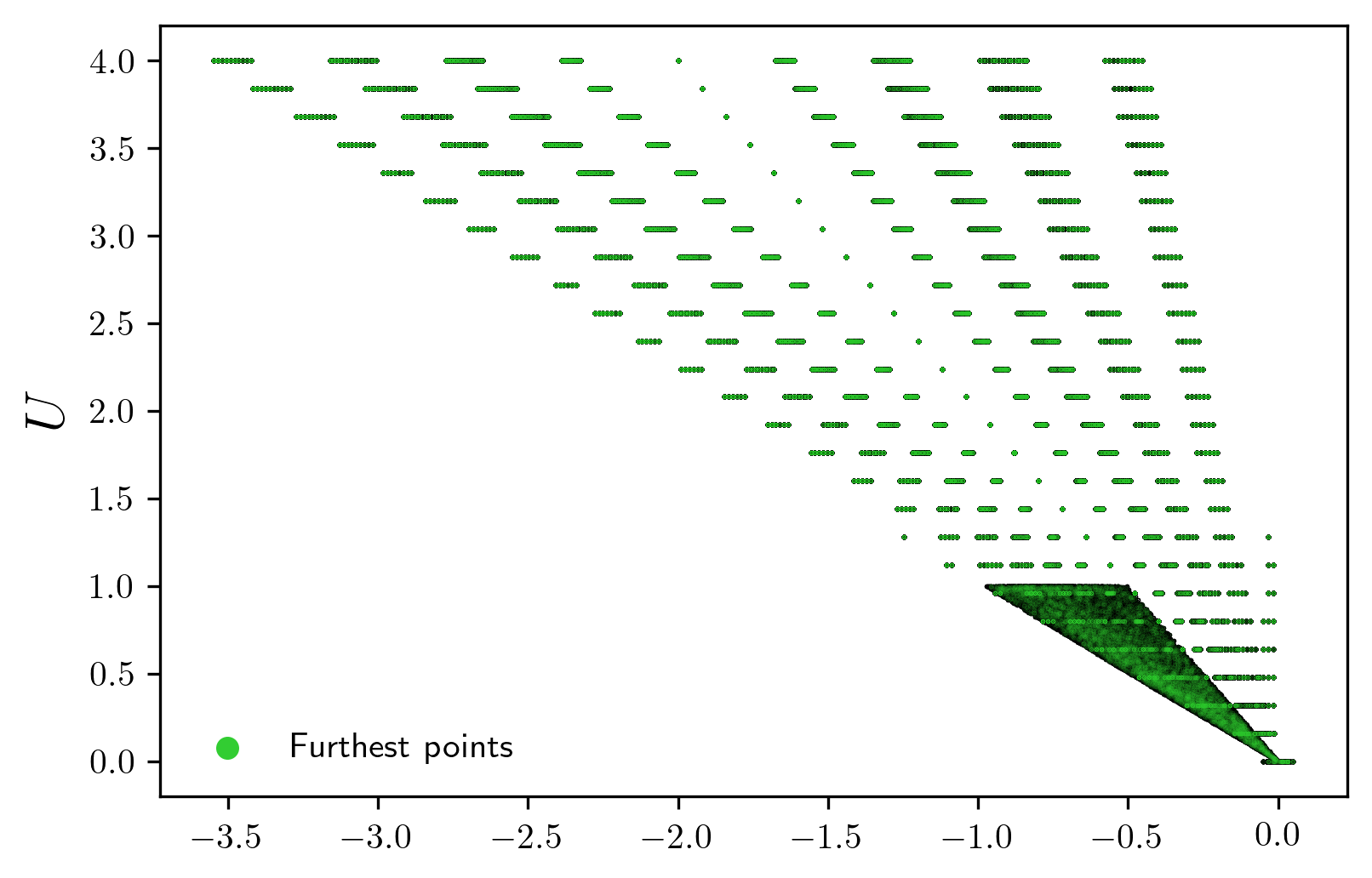
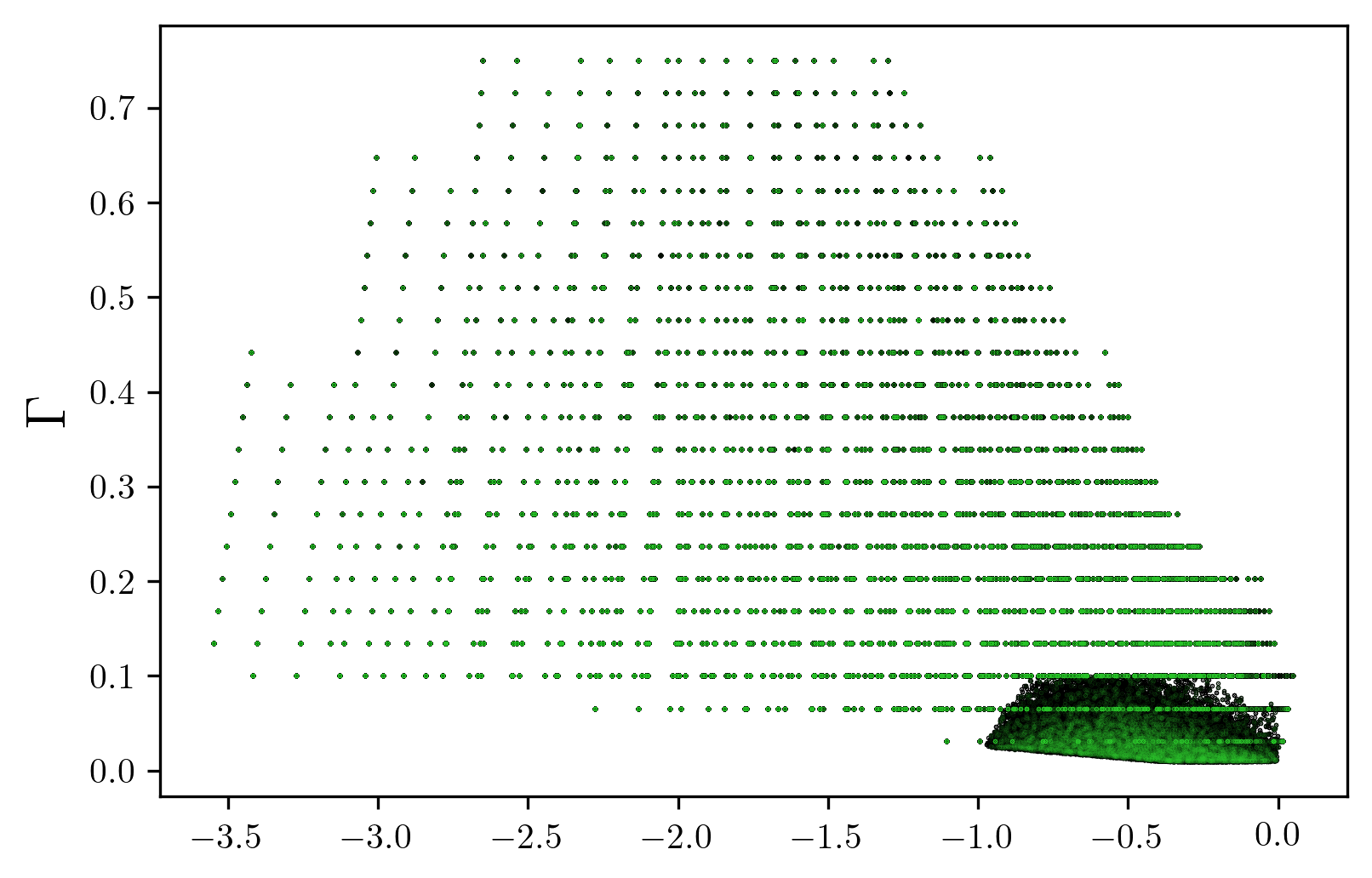
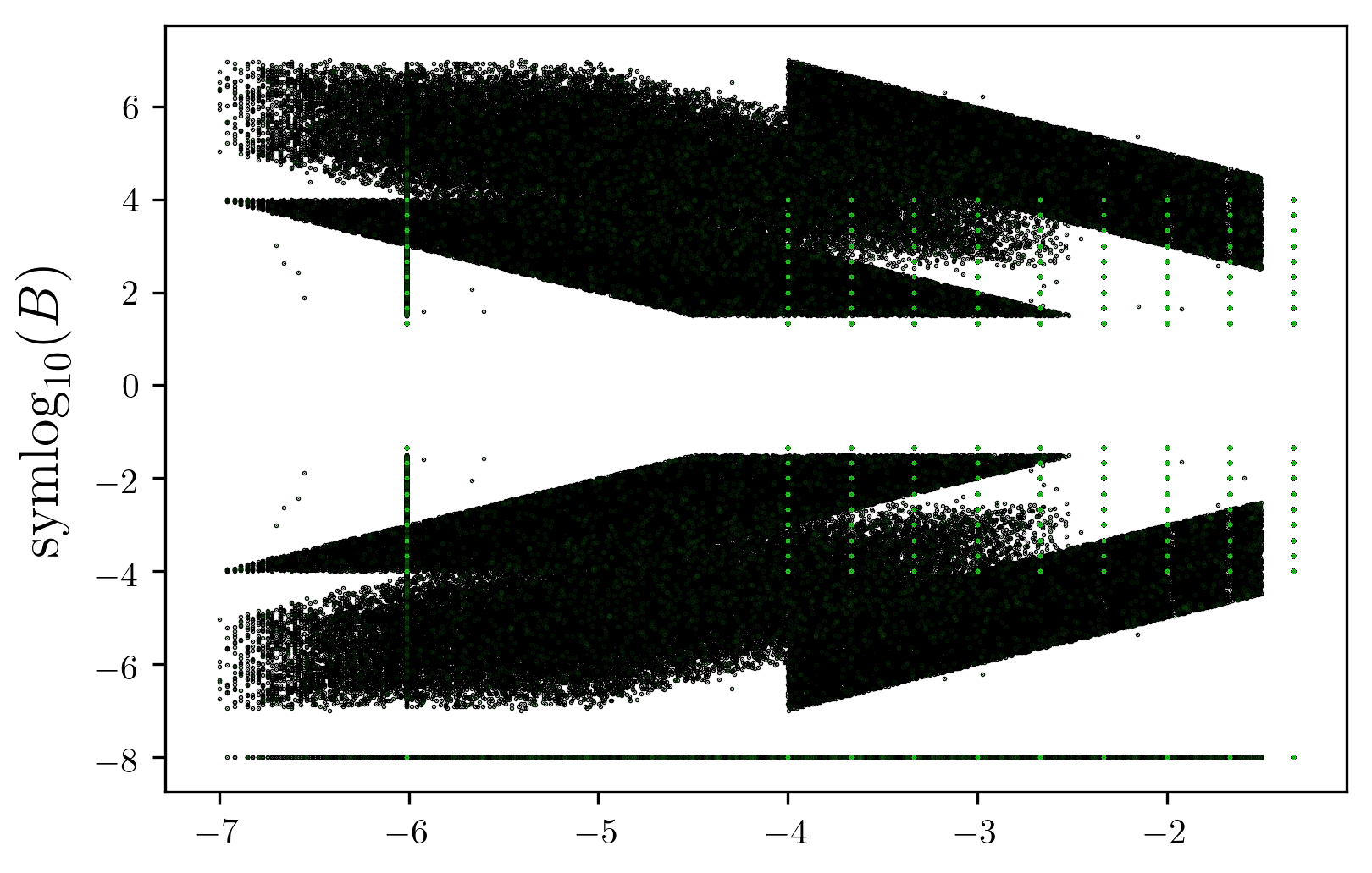
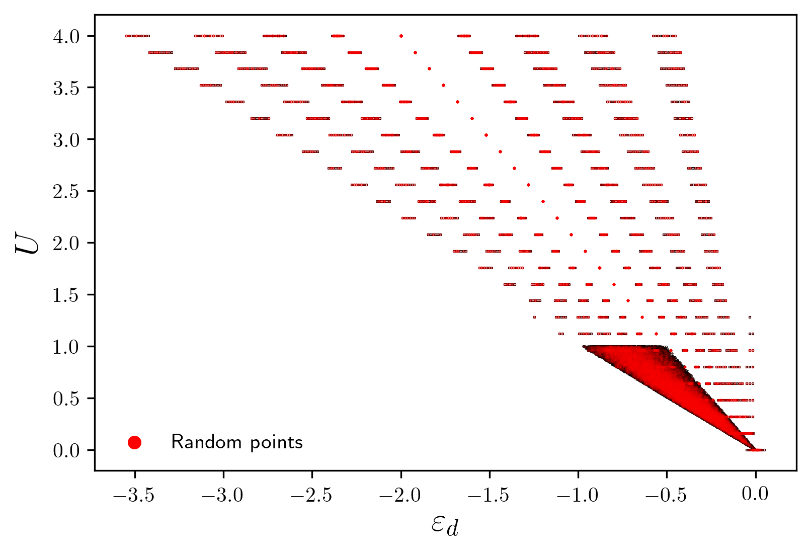
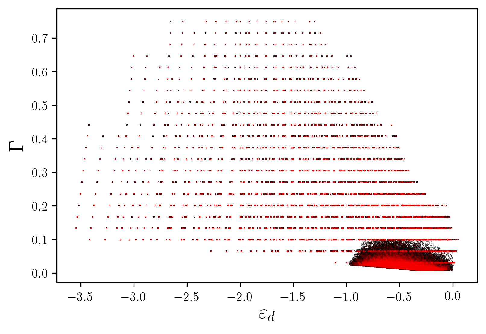
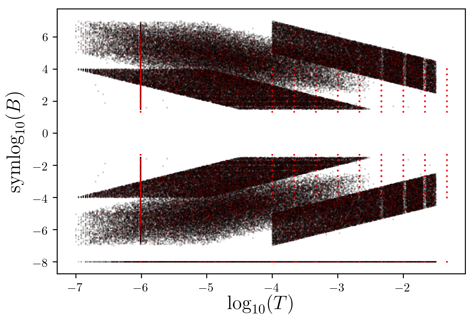
Figure A5: The input feature distribution for the full Kondo set (black). The down-sampled subsets each representing about 10% of the full data set are superimposed in color at 10% opacity to demonstrate density. The top row shows the furthest point algorithm’s subset in green, while the bottom row has the random point subset in red. See Sections A1.3 and A1.4 for additional information regarding the symmetric logarithm (symlog₁₀) procedure and furthest-point sampling algorithm respectively. The horizontal line at symlog${}_{10}(B)=-8$ in the right-most panels is caused by setting our $B\equiv 0\to 10^{-8}$ as explained in Section A1.3.

A0 A2: Machine learning models

In this section, we provide a brief overview of some machine learning theory, along with details of the specific model architectures and hyperparameters chosen in this work. For a detailed overview of practical machine learning technique in the domains of physics and chemistry, we refer the interested reader to the overview by Wang et al. Wang et al. (2020) and for details on feed-forward neural networks, to the overview by Cheng and Titterington Cheng and Titterington (1994). For details regarding the analytical models, see texts by Mohri et al. Mohri et al. (2018) and Hastie et al. Hastie et al. (2009). For the particular applications of these methods explored in this work, we refer our readers to Zhang et al. Zhang et al. (2013) and You et al. You et al. (2018).

A1.A1.1  A2.1: Neural networks

In this work we use a fully-connected feed-forward neural network known as a multi-layer perceptron (MLP) as the sole deep learning model. An MLP consists of sequential layers of nodes, where each node takes as input the output from all previous layers, and outputs a single value, known as an activation. The activations of the $l$th layer are computed by the general matrix equation $\mathbf{a}^{l}=f(W^{l}\mathbf{a}^{l-1}),$ where $\mathbf{a}^{l}$ is the vector of activations from the $l$th layer. $W^{l}$ is the $l$th weight matrix mapping the output from the $(l-1)$th layer to the input of the $l$th layer. The function $f$ is called the activation function. It applies a differentiable, element-wise non-linearity to the output, allowing the weights to learn highly-nonlinear representations of the input, parameterized by the neural network weights. These weights are learned during training, in which a numerical optimization procedure tries to find the minimum distance between ground truth training data points and the predictions. The specific model hyperparameters, or non-learned parameters of the model, are discussed in Section A2.2.

A2.A2.2  A2.2: Neural network training

Here we present the training protocols we used to train and hyperparameter-tune the neural networks used in this work. We find the optimal set of hyperparameters by using a combination of grid search and hand-tuning. The best model is determined by training models with different hyperparameter combinations on the same training set, evaluating on the validation set $\mathcal{V}$, and selecting the model with the lowest MAE. That model, finally, is evaluated on the testing set $\mathcal{T}$ which yields the presented data, unless indicated otherwise.

A3.A3.3  A2.3: Common neural network training parameters

All models share the following hyperparameters:

• $||\cdot||_{L_{1}}$ loss, the mean absolute error (MAE).

• Adam optimizer Kingma and Ba (2014) with a starting learning rate of $10^{-3}.$

• ReLU activation function.

• A scheduler which decreases the learning rate when the validation loss plateaus. This scheduler has a patience of 10 epochs, decrease factor of 0.5, and minimum learning rate of $10^{-7}.$

• Training batch size of 16 384 ($2^{14}$).

• For simplicity, we constrain all hidden layers to be of the same size.

• Total of 5000 epochs.

A4.A4.4  A2.4: Best neural network hyperparameters

As evaluated on $\mathcal{V},$ we present the best hyperparameter combinations in Table A1. Note that hyperparameter tuning is a highly non-convex problem, and it is possible that better combinations exist.

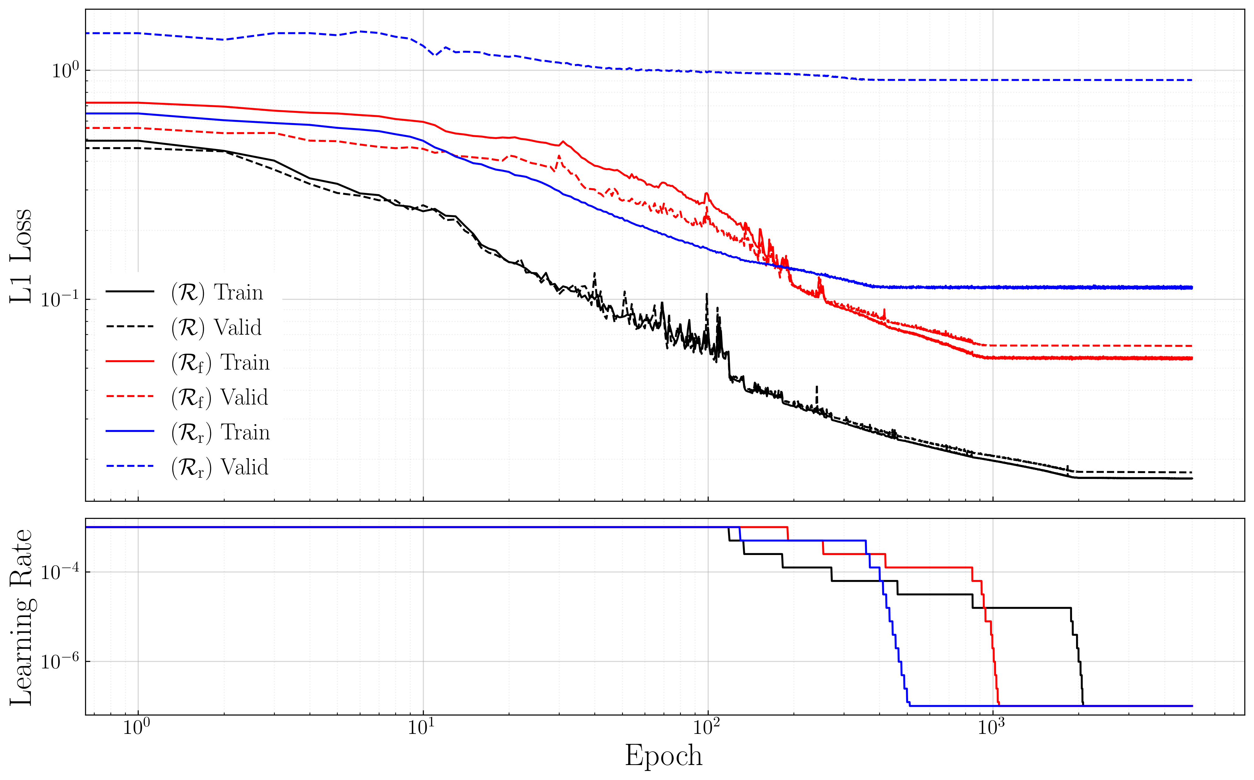
Figure A10: Anderson training and validation losses and learning rates plotted as a function of epochs for models trained on the full set $\mathcal{R},$ the FPS training set $\mathcal{R}_{\mathrm{f}},$ and random-sampled $\mathcal{R}_{\mathrm{r}},$ training sets.

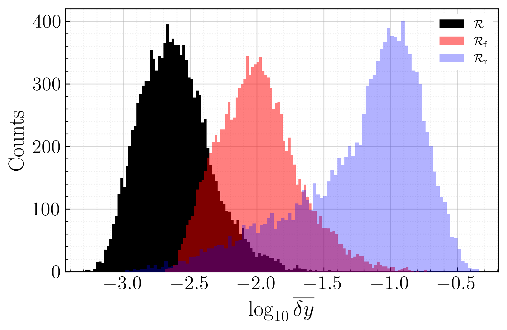
Figure A11: Anderson testing set histogram for the MLP models trained on the full $\mathcal{R},$ the FPS $\mathcal{R}_{\mathrm{f}},$ and random-sampled $\mathcal{R}_{\mathrm{r}}$ training sets.

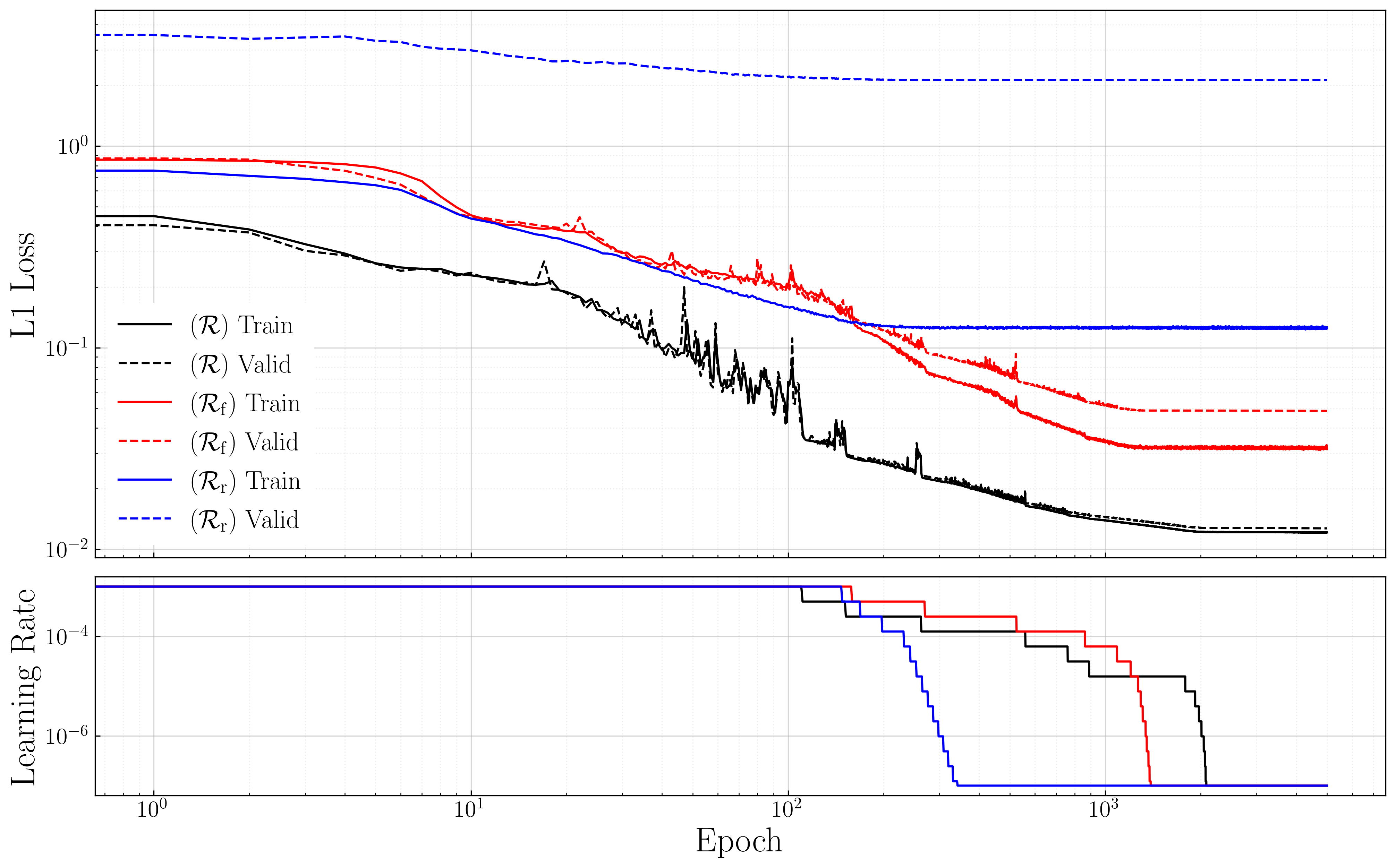
Figure A19: Kondo training and validation losses and learning rates plotted as a function of epochs for models trained on the full $\mathcal{R},$ FPS $\mathcal{R}_{\mathrm{f}},$ and random-sampled $\mathcal{R}_{\mathrm{r}}$ training sets.

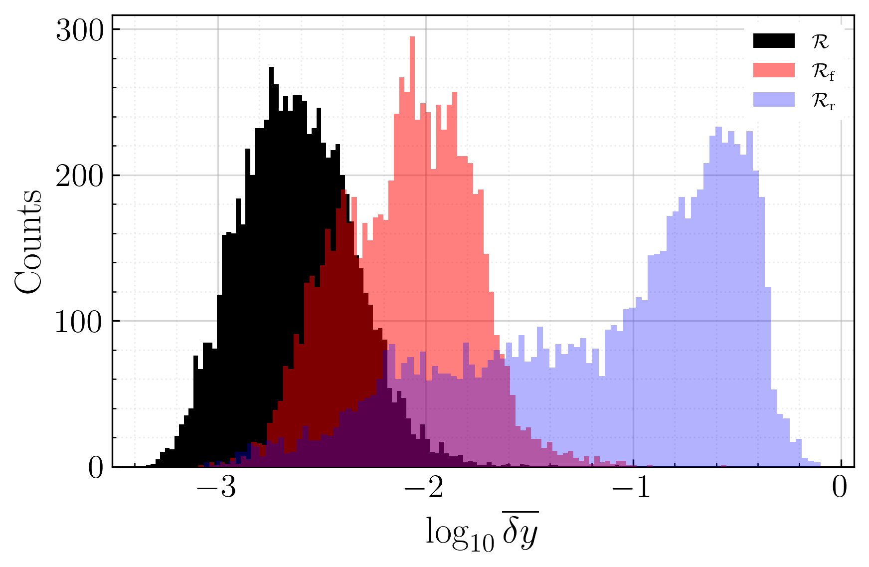
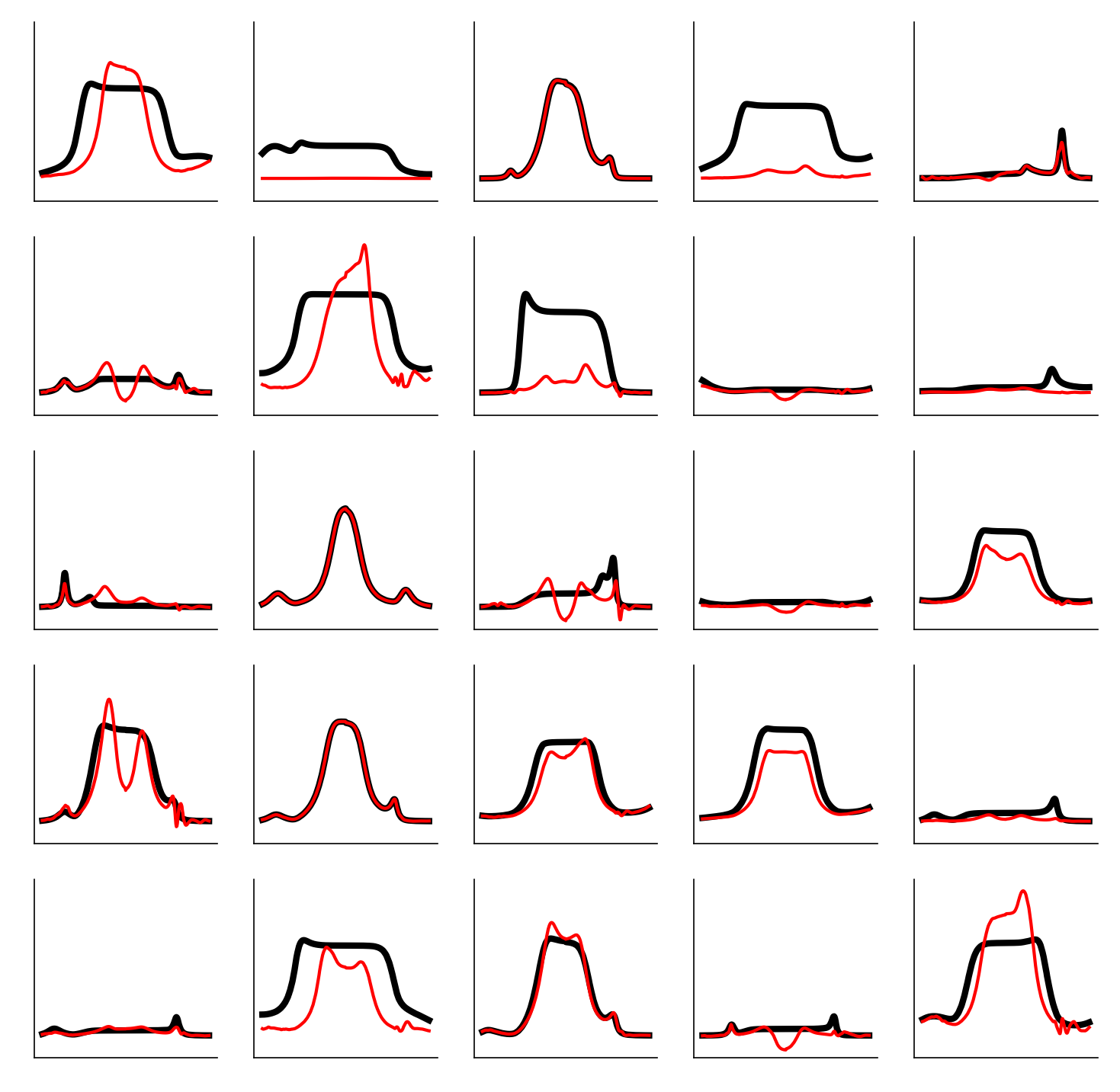
Figure A20: Kondo testing set histogram for the MLP models trained on the full $\mathcal{R},$ FPS $\mathcal{R}_{\mathrm{f}},$ and random-sampled $\mathcal{R}_{\mathrm{r}},$ training sets.

Table A1: The best hyperparameters for the neural networks for Anderson (upper rows) and Kondo (lower rows) as found by a combination of hand tuning and grid search. Training and validation losses are displayed in Fig. A10 and Fig. A19 for the Anderson and Kondo sets respectively. Testing set error distributions are shown in Fig. A11 and Fig. A20 for the Anderson and Kondo sets respectively. In the rightmost column (Examples), we provide the figure number where randomly drawn samples from each of the respective testing sets may be viewed. Both NRG ground truth (black) and predicted (red) spectra are displayed. Summaries of where the example results are shown are given in Tables A3 and A4.

Training set	hidden layer size	Number of hidden layers	Dropout Srivastava et al. (2014)	Examples
$\mathcal{R}^{\mathrm{A}}$	256	8	0	A7
$\mathcal{R}_{\mathrm{r}}^{\mathrm{A}}$	256	4	0.05	A8
$\mathcal{R}_{\mathrm{f}}^{\mathrm{A}}$	256	8	0	A9
$\mathcal{R}^{\mathrm{K}}$	256	8	0	A16
$\mathcal{R}_{\mathrm{r}}^{\mathrm{K}}$	256	4	0.05	A17
$\mathcal{R}_{\mathrm{f}}^{\mathrm{K}}$	256	8	0	A18

A5.A5.5  A2.5: Kernel ridge regression

Regression methods are trained to find the line of best fit. However, not all problems lend themselves well to a linear-fit decision boundary. In those cases it may be easier to compute the parameters’ higher dimensional dual space by way of a kernel where a linear fit may now be possible Mohri et al. (2018). This approach is known as kernel ridge regression (KRR) You et al. (2018); Pedregosa et al. (2011).

For a given trial $\left(x_{p},y_{p}\right)$ of $N$ total trials, the generic form of a KRR minimization algorithm reads:

$$\min\limits_{\alpha}\frac{1}{N} \left(\sum_{p=1}^{N}\left(y_{p}-f_{p}\right)^{2}+\lambda\lVert f\rVert_{\mathcal{H}}^{2}\right)$$ (AA5.6a)

$$f_{p} =\sum_{p^{\prime}=1}^{N}\alpha_{p^{\prime}}k\left(x_{p^{\prime}},x_{p}\right)$$ (AA5.6b)

where the first term in Eq. AA5.6a is the usual linear regression mean squared error (MSE) cost function between the model’s kernel-based prediction $f_{p}$ and ground truth value $y_{p}$ Zhang et al. (2013). While several kernels exist, in this work we exclusively use the Laplacian kernel Rupp (2015) given by $K_{pp^{\prime}}\equiv k(x_{p},x_{p^{\prime}})=\mathrm{exp}\bigl{(}-\tfrac{1}{\sigma}\|x_{p}-x_{p^{\prime}}\|_{1}\bigr{)}$ with input feature vectors $x_{p}$ and $x_{p^{\prime}}$ (5-dimensional in this work). The exponential argument is the L1 norm (Manhattan Distance) divided by the kernel radius $\sigma>0$ which determines how similar $x_{p}$ is to $x_{p^{\prime}}$. The target vectors $y_{p}$ are of size $M=333$ in the present case.

The second term in Eq. (AA5.6a) is the regularization term which helps prevent over-fitting. It includes two factors: the strength $\lambda\geq 0$, and the Hilbert space norm $\lVert f\rVert_{\mathcal{H}}$ defined as $\lVert f\rVert_{\mathcal{H}}:=\langle f,f\rangle_{\mathcal{H}}^{\nicefrac{{1}}{{2}}}$. Zhang et al. (2013) Both the kernel radius $\sigma$ and regularization strength $\lambda$ are tunable hyperparameters. Table A2 shows the selected hand-tuned hyperparameters. In this work we find that scaling the data by a symmetric logarithm procedure for $B$, $T$, and $\Gamma$ only improved the analytical algorithm results when the model is fit to $\mathcal{R}_{\mathrm{r}}$. Hence, no such scaling is applied when training with $\mathcal{R}_{\mathrm{f}}$. Throughout, we apply the standard normalization of the data, such that mean and standard deviations of all training data are 0 and 1, respectively [cf. Section A1.3].

Solving Eq. (AA5.6) for the weight matrix $\alpha$ requires an expensive inversion of the kernel matrix, $k(x_{p},x_{p^{\prime}})$ which scales as $O(N^{3})$ in time and $O(N^{2})$ in memory for $N$ data points $(x_{p},y_{p})$. This expense can be mitigated in several ways, including the divide-and-conquer approach, detailed below. In this work all KRR trials were modelled on 50k training trials (see Section A3).

The $r^{2}$ score (R-squared) value determines the quality of a trained regression model. A perfect model would achieve $r^{2}=1$, so the closer a model is to 1, the better the fit. A score of $r^{2}=0$ indicates that a constant model predicts the same result regardless of input. A negative score indicates that the model is arbitrarily worse than a constant representing the mean value. In this work we found that it was possible to generate acceptable models for the furthest-point sampled training data $\mathcal{R}_{\mathrm{f}}$, but the models fit with random point sampled $\mathcal{R}_{\mathrm{r}}$ training set were so poor that they had negative $r^{2}$ values. Therefore, if training set size is a limiting factor for a brute-force affordable KRR model (here inverting a full matrix of dimension 50k), then one must chose the training set with great care.

A6.A6.6  A2.6: Divide-and-conquer kernel ridge regression

Divide-and-conquer kernel ridge regression (DC-KRR) is one of several approaches one may take to mitigate the poor scaling of a traditional KRR algorithm explained above Zhang et al. (2013). In DC-KRR the total number $N\approx 500k$ of training trials is subdivided into $S\sim 10$ subsets with an equal number $n\approx 50k$ training trials in each (with minor variations for the Kondo as compared to the Anderson set). Then, a separate KRR model is fitted for each, and the trained weights ($\alpha$ in Eq. (AA5.6)) are saved. After training, a prediction may be acquired by computing (for each subset) the product of the weights and the kernel of the queried value and subset’s training trials. The final results are averaged for the final prediction as shown in Eq. AA6.7.

Given input parameters $x_{P}$ corresponding to ground truth target $y_{P}$, one may obtain a DC-KRR prediction $\hat{y}_{P}$ via:

$$\hat{y}_{P}=\frac{1}{S}\sum_{s=1}^{S}\mathrm{ker}(\mathcal{R}_{f}^{s},x_{P})\alpha_{s}$$ (AA6.7)

where $\alpha_{s}$ is a matrix of the learned algorithm weights described in Eqn. AA5.6 and ker$(\mathcal{R}_{f}^{s},x_{P})$ indicates the kernel between all $x_{p}\in\mathcal{R}_{f}^{s}$ and the queried $x_{P}$ input. DC-KRR has hyperparameters $\lambda$ and $\sigma$ which function in the same manner as described in Section 2.5 and we use the Laplacian kernel here as well. Final hyperparameter values are given in Table A2, which are applied universally for all subsets. Fig. A6 shows the individual $r^{2}$ values for each subset in the DC-KRR algorithm, whereas the final averaged $r^{2}$ value is reported in Table A2.

This approach reduces the cost of training with all data points in $\mathcal{R}$ and making the approach easily parallelizable. However, the overall scaling has not changed in this implementation; DC-KRR simply permits the use of the full training set. Additionally, it should be noted that the composition of the individual subsets matters. As DC-KRR works by training a multitude of standard KRR models, the same pitfalls that can negatively affect a single KRR model can also detract from the individual DC-KRR subset models which are then averaged, thus potentially compounding the error. In this work we chose to apply the furthest- point ordering on the training data prior to splitting $\mathcal{R}$ set into equal sized subsets as the KRR trials performed better with this pre-processing step.

A7.A7.7  A2.7: Best KRR and DC-KRR hyperparameters

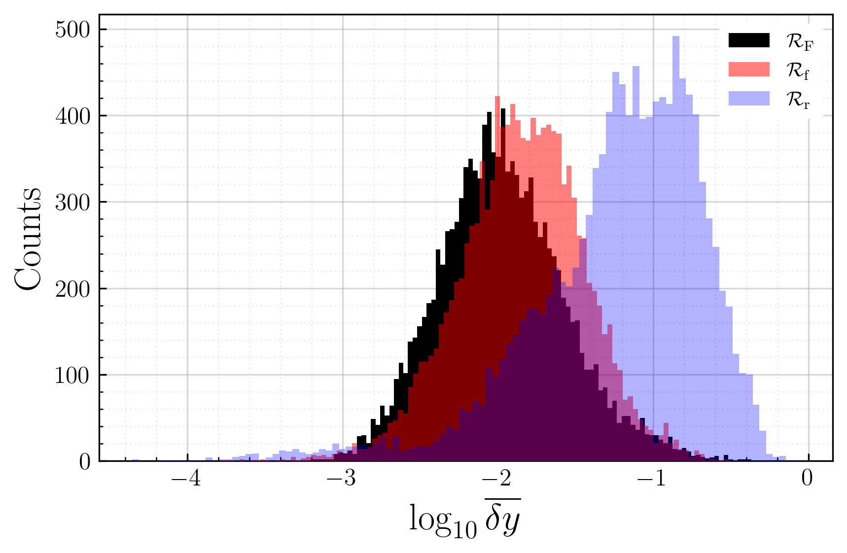
Figure A15: Anderson testing set histogram fro the DC-KRR trained with the chunked FPS-ordered set full $\mathcal{R}_{\mathrm{F}}$ (black), and the KRR models trained on the random $\mathcal{R}_{\mathrm{r}}$ (red) and FPS ordered $\mathcal{R}_{\mathrm{f}}$ (blue) down-sampled sets.

Table A2: The hand-tuned hyperparameters $\sigma$ and $\lambda$ [cf. Eqs. (AA5.6)], together with the $r^{2}$ scores of the validation ($\mathcal{V}$) and testing sets ($\mathcal{T}$) used in this work for kernel ridge regression (KRR) and divide-and-conquer KRR (DC-KRR). While several values were examined for each of these hyperparameters for each set of training data, only the final choices are presented. We also differentiate furthest-point sampled $\mathcal{R}_{\mathrm{f}}$ from random point sampled $\mathcal{R}_{\mathrm{r}}$ training data. For the training of the DC-KRR models, the full training set $\mathcal{R}$ was used, yet partitioned into $S$ disjoint subsets $\{\mathcal{R}_{f}^{s}\}$ as described in Eqn. 3 in the main text. Values for the DC-KRR $r^{2}$ entries are the result of averaging the $r^{2}$ values from the subsets shown in Fig. A6. In the rightmost column (Examples), we provide the figure number where randomly drawn samples from each of the respective testing sets may be viewed. Both NRG ground truth (black) and predicted (red) spectra are displayed. Summaries of where the example results are shown are given in Tables A3 and A4. Only the best models have associated result examples in Appendix A3. Figs. A15 and A24 demonstrate regression approach error distributions for the Anderson and Kondo sets respectively.

		Anderson						Kondo
KRR	Scaling	$\sigma$	$\lambda$	$r^{2}_{\mathcal{V}}$	$r^{2}_{\mathcal{T}}$	MAE($\mathcal{T}$)	Examples	$\sigma$	$\lambda$	$r^{2}_{\mathcal{V}}$	$r^{2}_{\mathcal{T}}$	MAE($\mathcal{T}$)	Examples
$\mathcal{R}_{\mathrm{r}}$	None	100	0	-0.267	-0.255	$0.102\pm 0.096$	N/A	100	0	-0.192	-0.204	$0.182\pm 0.187$	N/A
$\mathcal{R}_{\mathrm{r}}$	Symlog	$6.\bar{6}$	0.1	0.277	0.282	$0.085\pm 0.068$	A12	10	0	0.179	0.188	$0.152\pm 0.145$	A21
$\mathcal{R}_{\mathrm{f}}$	None	1	0.01	0.929	0.932	$0.021\pm 0.023$	A13	1	0.01	0.979	0.979	$0.019\pm 0.021$	A22
$\mathcal{R}_{\mathrm{f}}$	Symlog	1	0	0.909	0.915	$0.024\pm 0.026$	N/A	1	0.01	0.972	0.972	$0.023\pm 0.024$	N/A
DC-KRR
$\mathcal{R}_{\mathrm{F}}$	None	1	0	0.950	0.950	$0.0175\pm 0.026$	A14	1	0	0.902	0.899	$0.035\pm 0.033$	A23

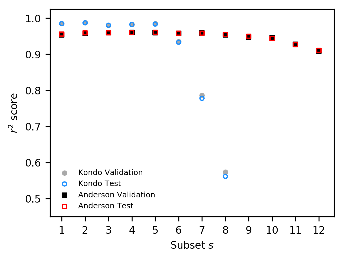
Figure A6: DC-KRR $r^{2}$ values for each subset within the Anderson (squares) and Kondo (circles) $\mathcal{R}_{\mathrm{F}}$ sets. Closed markers indicate the validation $r^{2}$ scores, and open markers indicate that of the test sets. Final DC-KRR values are the averages across all relevant subsets.

In Fig. A6 we present the $r^{2}$ values for each subset $s$ for the validation $\mathcal{V}$ and testing $\mathcal{T}$ sets in DC-KRR. In all cases there is excellent agreement between a given subset’s $r^{2}$ score for the validation and test sets. By the very construction of the underlying FPS, the last group ($s=S$) collects the rest of the data set, hence is no longer strictly FPS. This introduces a certain bias towards late patches, as seen in Fig. A6. The values for the Anderson set are tightly distributed. In contrast, the Kondo sets exhibit significant deterioration towards the last subsets $s=7$ and 8, negatively impacting the overall average. Despite this deterioration, however, the final $r^{2}$ values remain quite high for both datasets, indicating reliable models.

A0 A3: Results

In this section, we present figures demonstrating various representations of each model’s performance. These figures are connected to the different models in Table A3 for the Anderson results, and Table A4 for the Kondo results. For clarity, we highlight the differences between each dataset; note that all results that follow were hyperparameter-tuned on the same $\mathcal{V}$ and all results that follow in this section correspond to the testing set ($\mathcal{T}$) results as evaluated on the best model, which is determined by the MAE on $\mathcal{V}$.

• The full training set refers to training on all available training data, $\mathcal{R}$.

• The FPS training set refers to training on only the 50k furthest-points sampled data, $\mathcal{R}_{\mathrm{f}}=\mathcal{R}_{\mathrm{f}}^{(1)}.$

• The dataset $\mathcal{R}_{\mathrm{r}}$ refers to training on only the 50k randomly down-sampled data,

For all datasets, we present the following results:

• Random 25: a randomly-selected 25 samples plotted on the ML grid.

• Training info: loss and learning rate plots when applicable.

• Distribution: error distributions.

Table A3: A quick-reference for the Anderson results presented in this section. The table entries are figure labels. See text for description for the three rows.

	MLP$(\mathcal{R})$	MLP$(\mathcal{R}_{\mathrm{r}})$	MLP$(\mathcal{R}_{\mathrm{f}})$	KRR$(\mathcal{R}_{\mathrm{r}})$	KRR$(\mathcal{R}_{\mathrm{f}})$	DC-KRR$(\mathcal{R}_{\mathrm{F}})$
Random 25	A7	A8	A9	A12	A13	A14
Training info	A10	A10	A10	$-$	$-$	$-$
Distribution	A11	A11	A11	A15	A15	A15

Table A4: A quick-reference for the Kondo results presented in this section. The table entries are figure labels. See text for description fo the three rows.

	MLP$(\mathcal{R})$	MLP$(\mathcal{R}_{\mathrm{r}})$	MLP$(\mathcal{R}_{\mathrm{f}})$	KRR$(\mathcal{R}_{\mathrm{r}})$	KRR$(\mathcal{R}_{\mathrm{f}})$	DC-KRR$(\mathcal{R}_{\mathrm{F}})$
Random 25	A16	A17	A18	A21	A22	A23
Training info	A19	A19	A19	$-$	$-$	$-$
Distribution	A20	A20	A20	A24	A24	A24

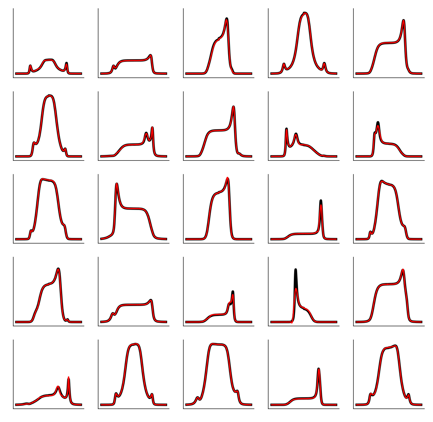
Figure A7: Random samples on the Anderson testing set for an MLP trained on $\mathcal{R}.$ Black is ground truth and red is prediction.

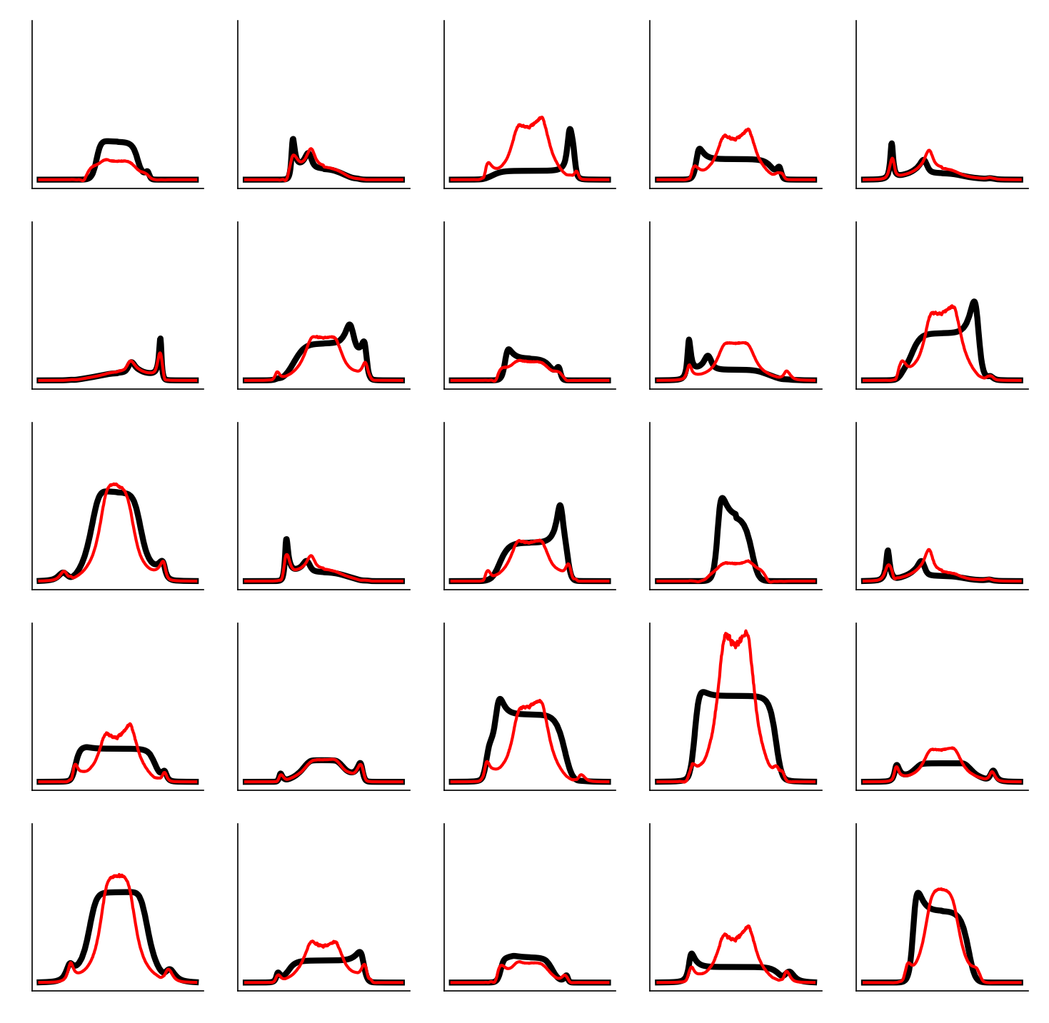
Figure A8: Random samples on the Anderson testing set for an MLP trained on $\mathcal{R}_{\mathrm{r}}.$ Black is ground truth and red is prediction.

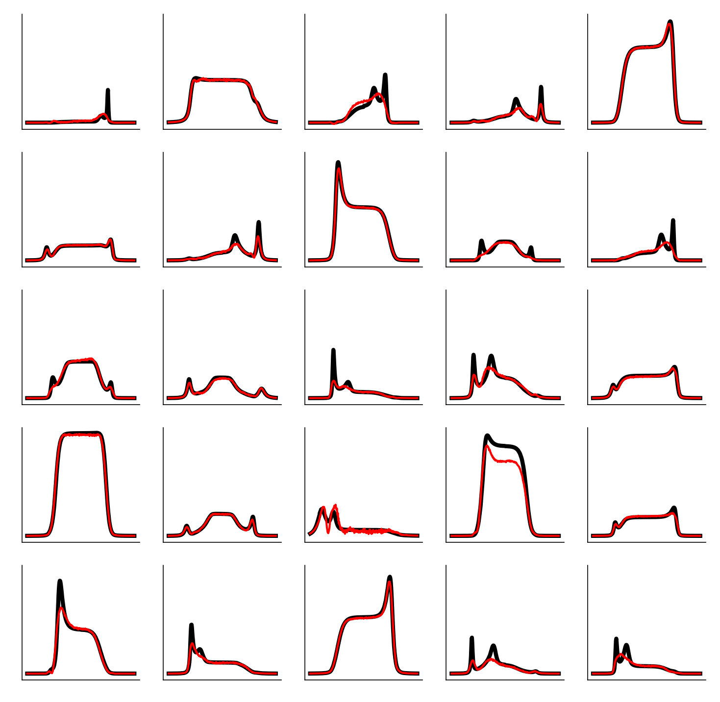
Figure A9: Random samples on the Anderson testing set for an MLP trained on $\mathcal{R}_{\mathrm{f}}.$ Black is ground truth and red is prediction.

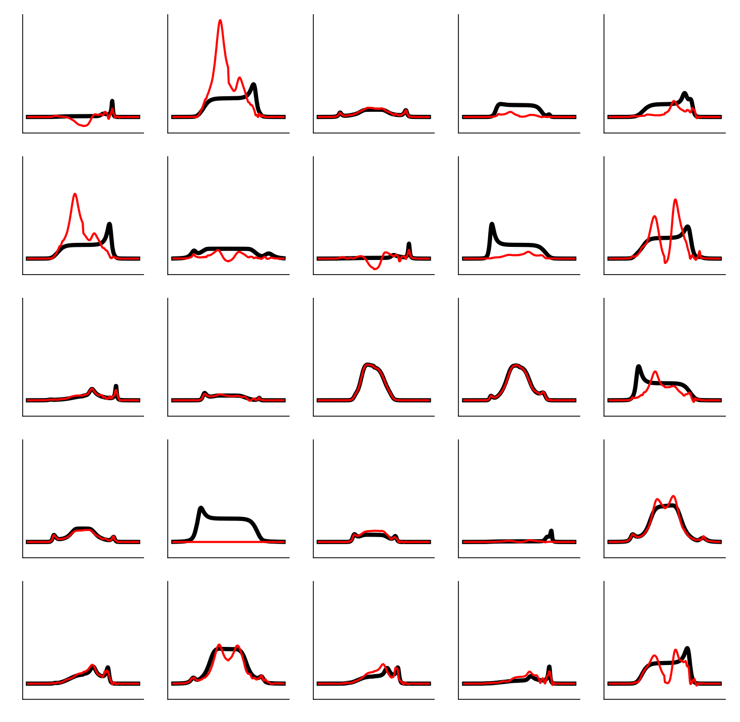
Figure A12: Random samples on the Anderson testing set for the KRR method trained on $\mathcal{R}_{\mathrm{r}}.$ Black is ground truth and red is prediction.

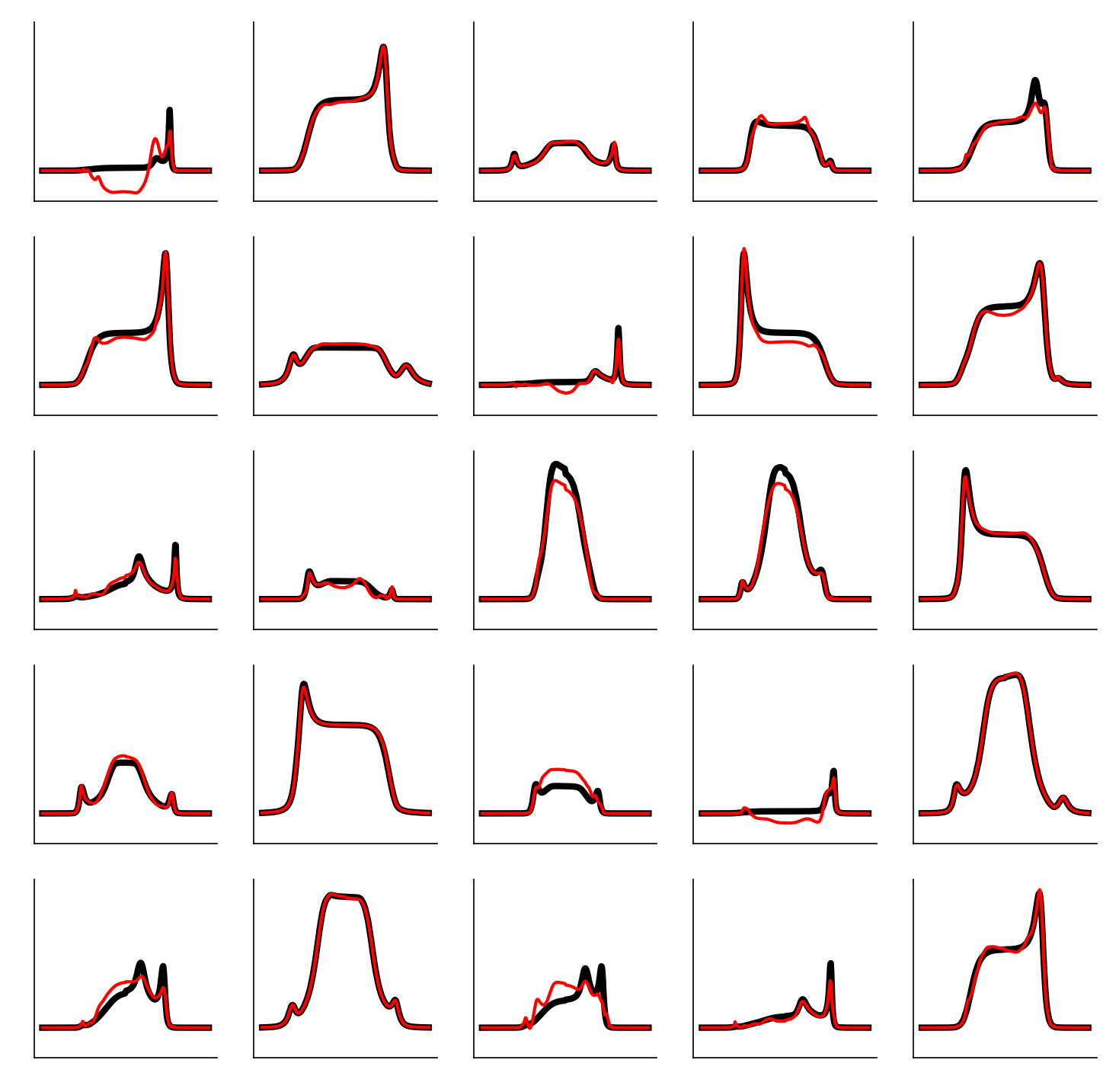
Figure A13: Random samples on the Anderson testing set for the KRR method trained on $\mathcal{R}_{\mathrm{f}}.$ Black is ground truth and red is prediction.

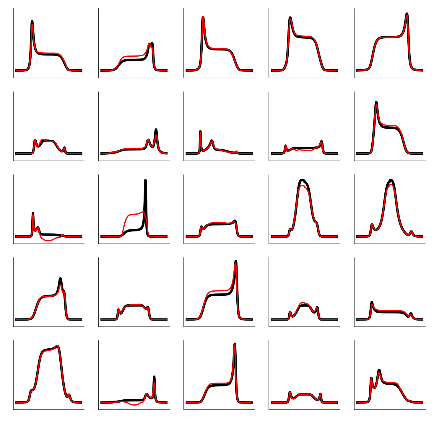
Figure A14: Random samples on the Anderson testing set for the DC-KRR method trained on $\mathcal{R}_{\mathrm{F}}.$ Black is ground truth and red is prediction. Note that the full training set is used, but the data is chunked in the order of the FPS data points.

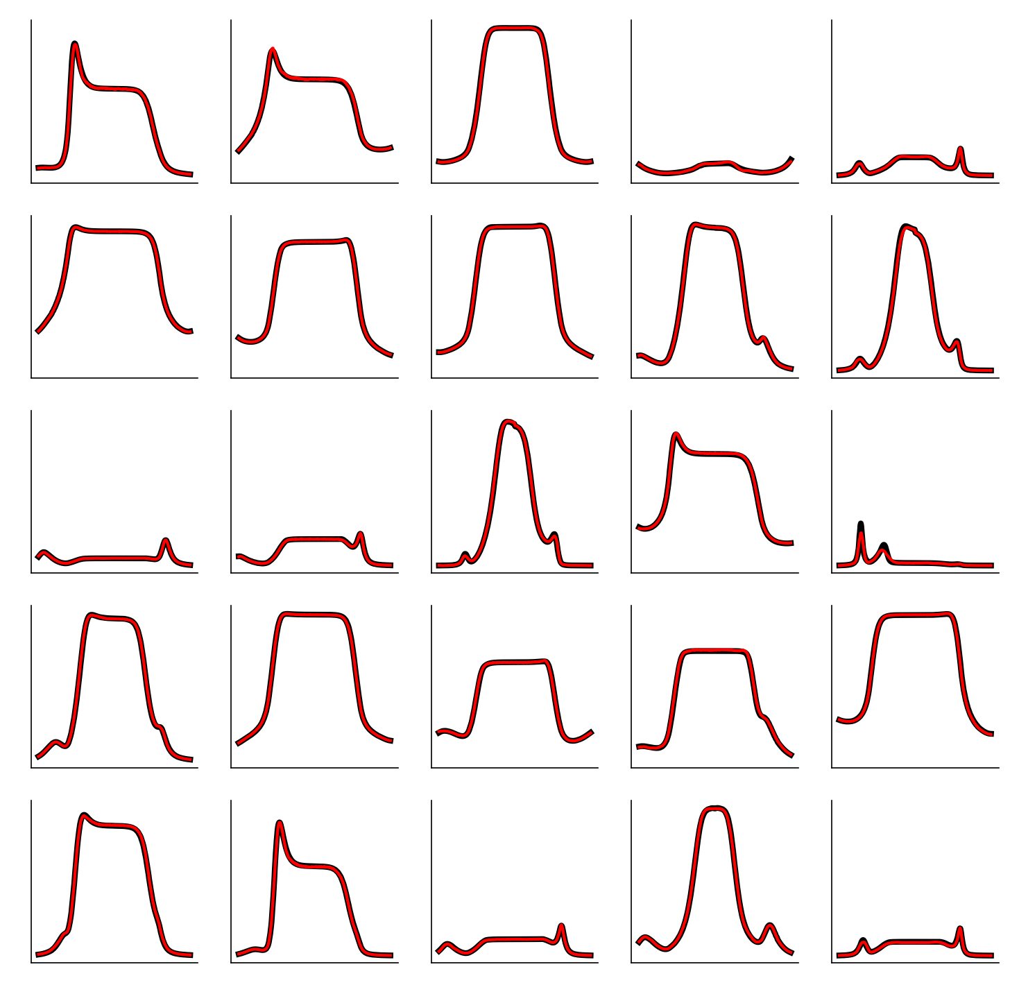
Figure A16: Random samples on the Kondo testing set for an MLP trained on $\mathcal{R}.$ Black is ground truth and red is prediction.

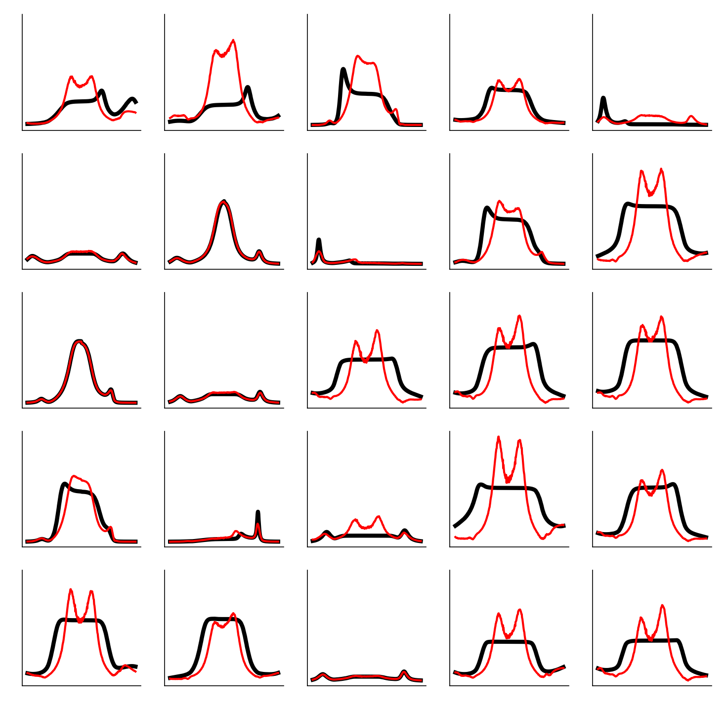
Figure A17: Random samples on the Kondo testing set for an MLP trained on $\mathcal{R}_{\mathrm{r}}.$ Black is ground truth and red is prediction.

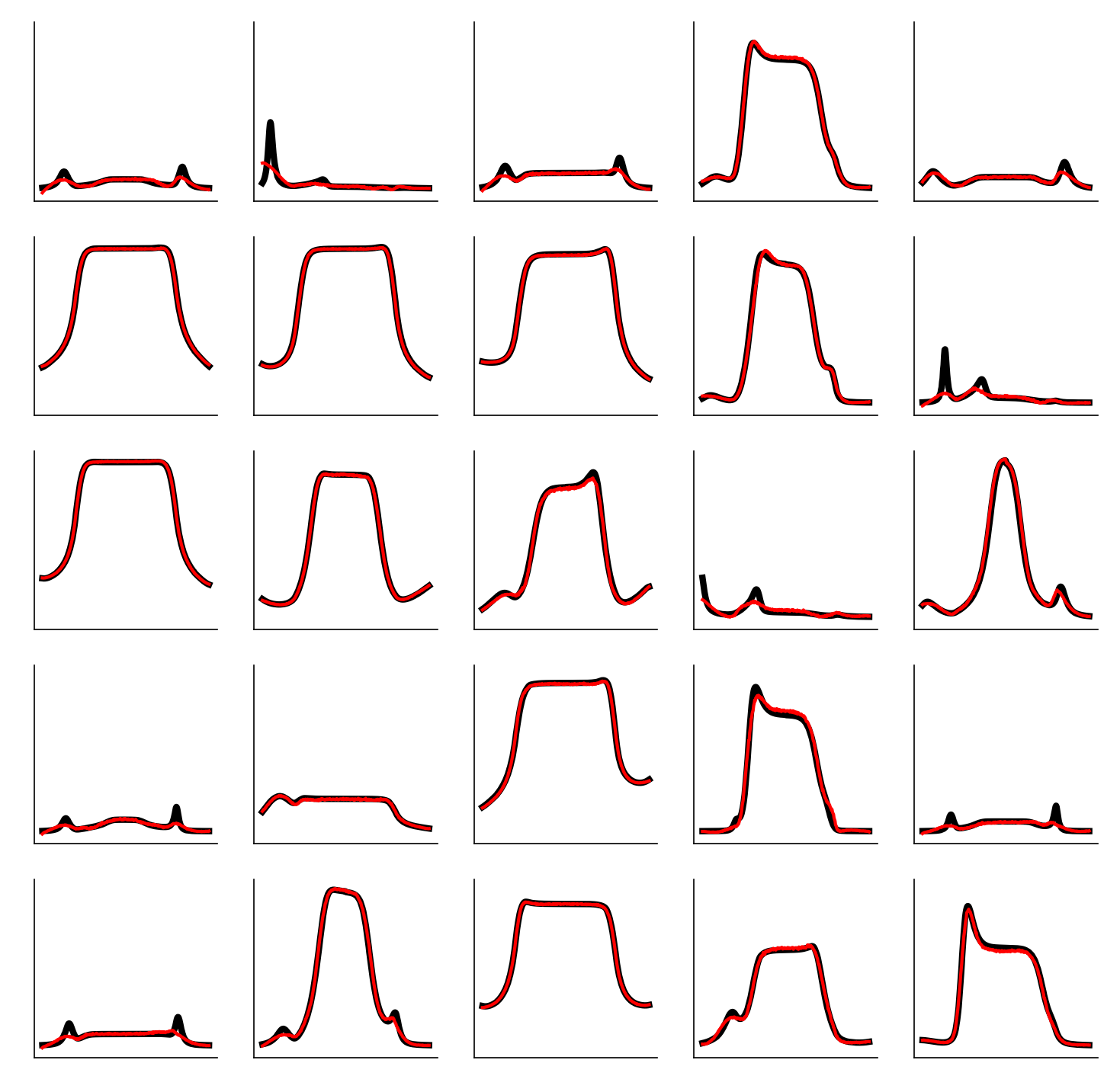
Figure A18: Random samples on the Kondo testing set for an MLP trained on $\mathcal{R}_{\mathrm{f}}.$ Black is ground truth and red is prediction.

Figure A21: Random samples on the Kondo testing set for the KRR method trained on $\mathcal{R}_{\mathrm{r}}.$ Black is ground truth and red is prediction.

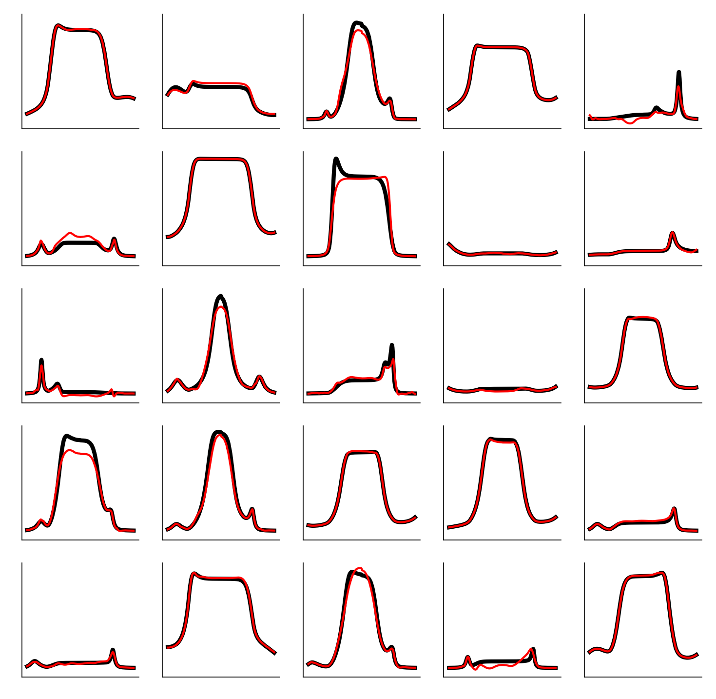
Figure A22: Random samples on the Kondo testing set for the KRR method trained on $\mathcal{R}_{\mathrm{f}}.$ Black is ground truth and red is prediction.

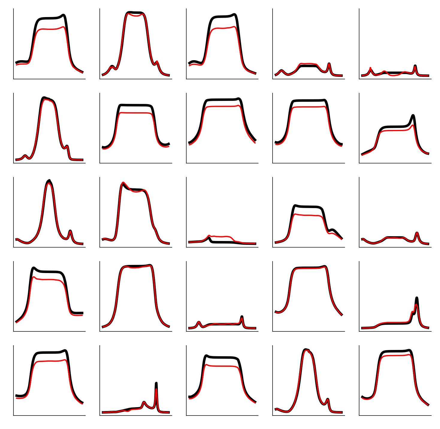
Figure A23: Random samples on the Kondo testing set for the DC-KRR method trained on $\mathcal{R}_{\mathrm{F}}.$ Black is ground truth and red is prediction. Note that the full training set is used, but the data is chunked in the order of the FPS data points.

Figure A24: Kondo testing set histogram fro the DC-KRR trained with the chunked FPS-ordered full set $\mathcal{R}_{\mathrm{F}}$ (black), and the KRR models trained on the random $\mathcal{R}_{\mathrm{r}}$ (red) and FPS ordered $\mathcal{R}_{\mathrm{f}}$ (blue) down-sampled sets.

References

- Lee et al. (2006) P. A. Lee, N. Nagaosa, and X.-G. Wen, Rev. Mod. Phys. 78, 17 (2006).
- Fradkin et al. (2015) E. Fradkin, S. A. Kivelson, and J. M. Tranquada, Rev. Mod. Phys. 87, 457 (2015).
- Ramirez (1997) A. P. Ramirez, J. Phys. Condens. Matter 9, 8171 (1997).
- Si and Steglich (2010) Q. Si and F. Steglich, Science 329, 1161 (2010).
- Homes et al. (2018) C. C. Homes, Q. Du, C. Petrovic, W. H. Brito, S. Choi, and G. Kotliar, Sci. Rep. 8 (2018).
- Chikina et al. (2020) A. Chikina, J.-Z. Ma, W. H. Brito, S. Choi, P. Sémon, A. Kutepov, Q. Du, J. Jandke, H. Liu, N. C. Plumb, M. Shi, C. Petrovic, M. Radovic, and G. Kotliar, Phys. Rev. Research 2, 023190 (2020).
- McMahan et al. (1998) A. McMahan, C. Huscroft, R. Scalettar, and E. Pollock, J. Comput. Aided Mol. Des. 5, 131 (1998).
- Metzner and Vollhardt (1989) W. Metzner and D. Vollhardt, Phys. Rev. Lett. 62, 324 (1989).
- Georges et al. (1996) A. Georges, G. Kotliar, W. Krauth, and M. J. Rozenberg, Rev. Mod. Phys. 68, 13 (1996).
- Kent and Kotliar (2018) P. R. C. Kent and G. Kotliar, Science 361, 348 (2018).
- de Haas et al. (1934) W. J. de Haas, J. de Boer, and G. J. van dën Berg, Physica 1, 1115 (1934).
- Costi et al. (2009) T. A. Costi, L. Bergqvist, A. Weichselbaum, J. von Delft, T. Micklitz, A. Rosch, P. Mavropoulos, P. H. Dederichs, F. Mallet, L. Saminadayar, and C. Bäuerle, Phys. Rev. Lett. 102, 056802 (2009).
- Leggett et al. (1987) A. J. Leggett, S. Chakravarty, A. T. Dorsey, M. P. A. Fisher, A. Garg, and W. Zwerger, Rev. Mod. Phys. 59, 1 (1987).
- Cronenwett et al. (1998) S. M. Cronenwett, T. H. Oosterkamp, and L. P. Kouwenhoven, Science 281, 540 (1998).
- Latta et al. (2011) C. Latta, F. Haupt, M. Hanl, A. Weichselbaum, M. Claassen, W. Wuester, P. Fallahi, S. Faelt, L. Glazman, J. v. Delft, H. E. Türeci, and A. Imamoglu, Nature 474, 627 (2011).
- Drozdov et al. (2014) I. K. Drozdov, A. Alexandradinata, S. Jeon, S. Nadj-Perge, H. Ji, R. J. Cava, B. A. Bernevig, and A. Yazdani, Nat. Phys. 10, 664 (2014).
- Anderson (1970) P. W. Anderson, Journal of Physics C: Solid State Physics 3, 2436 (1970).
- Kondo (1964) J. Kondo, Progress of Theoretical Physics 32, 37 (1964).
- Gull et al. (2011) E. Gull, A. J. Millis, A. I. Lichtenstein, A. N. Rubtsov, M. Troyer, and P. Werner, Rev. Mod. Phys. 83, 349 (2011).
- Aoki et al. (2014) H. Aoki, N. Tsuji, M. Eckstein, M. Kollar, T. Oka, and P. Werner, Rev. Mod. Phys. 86, 779 (2014).
- Wilson (1975) K. G. Wilson, Rev. Mod. Phys. 47, 773 (1975).
- White (1992) S. R. White, Phys. Rev. Lett. 69, 2863 (1992).
- Melnick et al. (2020) C. Melnick, P. Sémon, K. Yu, N. D’Imperio, A.-M. Tremblay, and G. Kotliar, “Accelerated impurity solver for dmft and its diagrammatic extensions,” (2020), ArXiv:2010.08482 [cond-mat.str-el] .
- Arsenault et al. (2014) L.-F. Arsenault, A. Lopez-Bezanilla, O. A. von Lilienfeld, and A. J. Millis, Phys. Rev. B 90, 155136 (2014).
- Walker et al. (2020) N. Walker, S. Kellar, Y. Zhang, and K.-M. Tam, “Neural network solver for small quantum clusters,” (2020), arXiv:2008.12331 [cond-mat.str-el] .
- Bulla et al. (2008) R. Bulla, T. A. Costi, and T. Pruschke, Rev. Mod. Phys. 80, 395 (2008).
- Anders and Schiller (2005) F. B. Anders and A. Schiller, Phys. Rev. Lett. 95, 196801 (2005).
- Weichselbaum and von Delft (2007) A. Weichselbaum and J. von Delft, Phys. Rev. Lett. 99, 076402 (2007).
- Stadler et al. (2015) K. M. Stadler, Z. P. Yin, J. von Delft, G. Kotliar, and A. Weichselbaum, Phys. Rev. Lett. 115, 136401 (2015).
- Lee et al. (2017) S.-S. B. Lee, J. von Delft, and A. Weichselbaum, Phys. Rev. Lett. 119, 236402 (2017).
- Anderson (1961) P. W. Anderson, Phys. Rev. 124, 41 (1961).
- Rigo and Mitchell (2020) J. B. Rigo and A. K. Mitchell, Phys. Rev. B 101, 241105 (2020).
- Hendry and Feiguin (2019) D. Hendry and A. E. Feiguin, Phys. Rev. B 100, 245123 (2019).
- (34) “Supplemental Material (url will be inserted by publisher).” .
- Note (1) The Anderson and Kondo data sets are completely disjoint, i.e., they have separate training, validation and testing sets, and are independently trained and evaluated. As such we often suppress the index for brevity.
- Pedregosa et al. (2011) F. Pedregosa, G. Varoquaux, A. Gramfort, V. Michel, B. Thirion, O. Grisel, M. Blondel, P. Prettenhofer, R. Weiss, V. Dubourg, J. Vanderplas, A. Passos, D. Cournapeau, M. Brucher, M. Perrot, and E. Duchesnay, J. Mach. 12, 2825 (2011).
- Zhang et al. (2013) Y. Zhang, J. C. Duchi, and M. J. Wainwright, J. Mach. 16, 3299 (2013).
- You et al. (2018) Y. You, J. Demmel, C.-J. Hsieh, and R. Vuduc, in Proceedings of the 2018 International Conference on Supercomputing - ICS ’18 (ACM Press, New York, New York, USA, 2018) pp. 307–317.
- Bulla et al. (1998) R. Bulla, A. C. Hewson, and T. Pruschke, J. Phys. Condens. Matter 10, 8365 (1998).
- Meir et al. (1991) Y. Meir, N. S. Wingreen, and P. A. Lee, Phys. Rev. Lett. 66, 3048 (1991).
- Goldhaber-Gordon et al. (1998) D. Goldhaber-Gordon, H. Shtrikman, D. Mahalu, D. Abusch-Magder, U. Meirav, and M. A. Kastner, Nature 391, 156 (1998).
- Haldane (1978) F. D. M. Haldane, Phys. Rev. Lett. 40, 416 (1978).
- Wang et al. (2020) A. Y.-T. Wang, R. J. Murdock, S. K. Kauwe, A. O. Oliynyk, A. Gurlo, J. Brgoch, K. A. Persson, and T. D. Sparks, Chem. Mater. (2020).
- Cheng and Titterington (1994) B. Cheng and D. M. Titterington, Stat. Sci 9, 2 (1994).
- Mohri et al. (2018) M. Mohri, A. Rostamizadeh, and A. Talwalkar, Foundations of Machine Learning, 2nd ed. (The MIT Press, Cambridge, MA, 2018).
- Hastie et al. (2009) T. Hastie, R. Tibshirani, and J. Friedman, The Elements of Statistical Learning: Data Mining, Inference, and Prediction, 2nd ed. (Springer-Verlag, New York, New York, USA, 2009).
- Note (2) We remind the reader that the validation and testing sets are fixed for each for the entirety of this work.
- Kingma and Ba (2014) D. P. Kingma and J. Ba, arXiv preprint arXiv:1412.6980 (2014).
- Srivastava et al. (2014) N. Srivastava, G. Hinton, A. Krizhevsky, I. Sutskever, and R. Salakhutdinov, The journal of machine learning research 15, 1929 (2014).
- Rupp (2015) M. Rupp, Int. J. Quantum Chem. 115, 1058 (2015).