Strain localization regularization and patterns formation in rate-dependent plastic materials with multiphysics coupling

Abstract

Strain localization is an instability phenomenon occurring in deformable solid materials which undergo dissipative deformation mechanisms. Such instability is characterized by the localization of the displacement or velocity fields in a zone of finite thickness and is generally associated with the failure of materials. In several fields of material engineering and natural sciences, estimating the thickness of localized deformation is required to make accurate predictions of the evolution of the physical properties within localized strain regions and of the material strength. In this context, scientists and engineers often rely on numerical modeling techniques to study strain localization in solid materials. However, classical continuum theory for elasto-plastic materials fails at estimating strain localization thicknesses due to the lack of an internal length in the model constitutive laws. In this study, we investigate at which conditions multiphysics coupling enables to regularize the problem of strain localization using rate-dependent plasticity. We show that coupling the constitutive laws for deformation to a single generic diffusion-reaction equation representing a dissipative state variable can be sufficient to regularize the ill-posed problem under some conditions on the softening parameters in the plastic potential. We demonstrate in these cases how rate-dependent plasticity and multiphysics coupling can lead to material instabilities depicting one or several internal length scales controlled by the physical parameters resulting in the formation of regular or erratic patterns. As we consider a general form of the equations, the results presented in this study can be applied to a large panel of examples in the material engineering and geosciences communities.

1 Introduction

Solid materials can undergo irreversible deformation mechanisms when subject to large deformation and consequently to large stresses. Such irreversible deformation is usually associated with the dissipation of some energy quantity which may depend on a set of coupled state variables such as temperature and pressure. In a large variety of solid materials undergoing irreversible deformation, the displacement and velocity fields can localize in finite thicknesses which are commonly described as strain localization phenomena. Understanding the conditions which lead to localization instabilities and how they evolve has become of relevance in several fields of material engineering and natural sciences as localization instabilities can drastically alter the physical properties of the solid materials and ultimately lead to its failure. Observations of localization instabilities are well documented by laboratory studies for a large variety of materials, including: (i) metals and alloys [Tresca, 1878, Antolovich & Armstrong, 2014]; (ii) biomaterials [Richman et al., 1975, Budday et al., 2014, Molnár et al., 2018]; or (iii) geomaterials [Desrues et al., 1996, Baud et al., 2004, Fossen et al., 2007]. To explain these observations, the scientific community has put forward several theoretical frameworks in the last decades [Rudnicki & Rice, 1975, Issen & Rudnicki, 2000]. One major outcome of this theoretical effort was to recognize that Cauchy-Boltzmann mechanical formulation, which is usually adopted to describe the deformation of solids fails at describing strain localization phenomena as it predicts localized thicknesses of zero-size [Iordache & William, 1998, Rattez et al., 2018a]. Such formulations are therefore said to be ill-posed as they induce mesh-dependency in finite-element analyses accompanied with convergence defects [Borst et al., 1993, Vardoulakis & Sulem, 1995, Rattez et al., 2018b]. To mitigate this effect, several regularization techniques are found in the literature, such as higher-order continuum theories [Mühlhaus & Vardoulakis, 1987, Pijaudier-Cabot & Bazant, 1987, Vardoulakis & Aifantis, 1991, Forest et al., 2005], multiphysics coupling [Benallal & Bigoni, 2004, Benallal, 2005, Rice et al., 2014, Veveakis et al., 2014b] or viscous regularization [Needleman, 1988, Loret & Prevost, 1990, Prevost & Loret, 1990, Wang et al., 1996].

The concept of viscous regularization of the strain localization problem was first introduced by Needleman [1988] and later followed by Prevost & Loret [1990], Loret & Prevost [1990] who described by means of numerical tests how rate-dependency resolves the mesh-dependency of strain localization for softening materials under quasi-static and dynamic loading conditions. As explained in [Bažant & Jirásek, 2002], the rate dependency introduces a characteristic length scale – only when the inertial terms are considered – which allows to prevent the change of type of partial differential equations that occurs with strain softening, rate independent materials and to regularize the strain localization problem. However, this regularization presents peculiarities compared to other regularization methods like high order continuum theories. Its effect tends to disappear in time if the time scale of the problem is larger than the relaxation time associated with the viscous terms. Thus, this viscous regularization can only be used within a narrow range of time delays and rates [Bažant & Jirásek, 2002]. Benallal [2008] later investigated the conditions in terms of loading conditions, viscosity and numerical time discretization for the regularization by viscous terms to be effective. Moreover, this rate-dependent regularization is more sensitive to the imperfections triggering the localization process than other methods [Molinari & Clifton, 1987, Belytschko et al., 1991]. Wang et al. [1996] have shown that the size of the strain localization zone is controlled by the minimum of the imperfection length scale and the viscous length scale, that is why recent numerical study have introduced a large perturbation length scale in their numerical setting to study localization in geomaterials [Duretz et al., 2014, 2019, Jacquey & Cacace, 2020]. In his seminal paper, Needleman [1988] also noticed that the length scale of strain localization is related to heterogeneities or imperfections and speculated that considering additional coupling to diffusive processes would integrate a physical length scale into the constitutive laws of deformation. This coupling of rate-dependency and a diffusion equation has been applied to study the phenomenon of adiabatic shear bands [Batra & Kim, 1991, McAuliffe & Waisman, 2013] for the particular case of the temperature-dependent mechanical behavior and it has been shown that for a variety of imperfections the shear-band structure depends almost entirely on the imposed nominal strain rate and material parameters [Bayliss et al., 1994]. However, all these studies have shown numerically the regularization by the viscous-diffusion coupling for a single or limited set of parameters, but it remains unclear under which conditions the coupling of a diffusion equation regularizes the problem of strain localization or how the viscous and diffusive characteristic lengths interact to control the localization for problems involving a small relaxation time compared to the viscous time scale.

To address these questions, we consider in this study a general combination of multiphysics coupling and viscous terms to investigate the regularization of the ill-posed problem. We performed a linear stability analysis of the resulting system of equations and demonstrate the conditions necessary to regularize the strain localization problem. We have identified several strain localization regimes based on the dependency of the plastic yield to accumulated plastic strain and coupled dissipative variable. Two specific regimes are covered in this study: one for which strain localization regularization induces the formation of regular patterns controlled by standing waves and another where the regularization can induce complex patterns controlled by the interplay of standing and propagating waves. We also present the dynamic evolution of such systems by means of finite-element simulations.

2 Problem formulation

In the following, we describe the mathematical formulation of the one-dimensional deformation of a solid material using a rate-dependent plasticity model coupled to a diffusion-reaction equation. Materials subject to pure shear, pure compression or uniaxial deformation can be reduced to one-dimensional problems but more complex loading conditions would require to account for additional dimensions. We make use of a classical additive splitting of the total strain ($\gamma$) into an elastic ($\gamma^{el}$) and a plastic component ($\gamma^{p}$):

$$\gamma=\frac{\partial u}{\partial x}=\gamma^{el}+\gamma^{p}$$ (1)

The governing equation for the displacement variable $u$ in one dimension is obtained based on the balance of momentum:

$$\rho\frac{\partial^{2}u}{\partial t^{2}}-\frac{\partial\tau}{\partial x}=\rho\frac{\partial^{2}u}{\partial t^{2}}-G\frac{\partial^{2}u}{\partial x^{2}}+G\frac{\partial\gamma^{p}}{\partial x}=0$$ (2)

where $G$ is the elastic modulus and $\rho$ the material density. Equation 2 is similar to a wave equation with an additional term depending on the plastic behavior of the material. Equation 2 can also be expressed by considering the velocity $v=\frac{\partial u}{\partial t}$ as the primary variable for deformation:

$$\frac{1}{c^{2}}\frac{\partial^{2}v}{\partial t^{2}}-\frac{\partial^{2}v}{\partial x^{2}}+\frac{\partial\dot{\gamma}^{p}}{\partial x}=0,$$ (3)

where $c=\sqrt{\frac{G}{\rho}}$ is the elastic wave velocity and $\dot{\gamma}^{p}$ the plastic strain rate. The plastic strain is generally considered as an internal variable and not a state variable. Additionally, we consider a coupled variable $\theta$ (here considered dimensionless for sake of generality) governed by a diffusion-reaction type of equation:

$$\frac{\partial\theta}{\partial t}-\kappa\frac{\partial^{2}\theta}{\partial x^{2}}-\alpha\dot{\gamma}^{p}=0,$$ (4)

where $\kappa$ is the diffusivity of the material and $\alpha$ a coefficient controlling the release of mechanical energy. We keep the coupled variable $\theta$ as a generic variable in this study as it can represent a large variety of processes depending of the type of material considered, the spatial and temporal scales at which we consider the deformation of the material and the type of forcing conditions the material is subject to. In a general sense, Equation 4 represents the diffusion of an internal quantity which is relevant for the deformation of the material. The variable $\theta$ could therefore represent physical quantities such as temperature of the material; the saturation or the fluid pressure in the case of fully-saturated porous media; the mass concentration of a specific mineral; or the microstructure organization representing a phase transition. This variable can also be interpreted as a non-local version of the accumulated plastic strain, in the form of a damage or breakage variable often adopted for granular media [Kamrin, 2019]. The source term $\alpha\dot{\gamma}^{p}$ is chosen to be generic, representing effects like the dissipation rate in the case of $\theta$ being the temperature, the volumetric plastic rate of deformation in mass balance considerations, the deviatoric plastic strain rate in the case of $\theta$ being a generalized damage variable expressing shear failure, to mention only a few examples. Here for sake of simplicity, we consider $\alpha=1$ but in a general sense this coefficient can be a function of stress, elastic strain or other state variables depending on the physics considered.

We consider the onset of plastic deformation as being controlled by the following yield function formulated in terms of stress:

$$\mathcal{F}=\tau-\tau_{y}\left(\gamma^{p},\theta\right)$$ (5)

where $\tau$ is the stress and $\tau_{y}$ the yield stress expressed as a function of the two variables $\gamma^{p}$ and $\theta$. Assuming a rate-dependent plastic model or viscoplastic (overstress) rheology, the flow law for the plastic strain is expressed as:

$$\dot{\gamma}^{p}=\frac{\langle\mathcal{F}\rangle}{\eta}\frac{\partial\mathcal{F}}{\partial\tau},$$ (6)

where $\eta$ is the material viscosity and $\langle x\rangle=\frac{x+\lvert x\rvert}{2}$ denotes the Macauley brackets. Using the expression of the function introduced in Equation 5, one can obtain the following flow rule for the viscoplastic strain:

$$\dot{\gamma}^{p}=\frac{G}{\eta}\langle\bar{\tau}-\bar{\tau}_{y}\left(\gamma^{p},\theta\right)\rangle,$$ (7)

where $\bar{\tau}=\frac{\tau}{G}$ and $\bar{\tau}_{y}=\frac{\tau_{y}}{G}$ are the dimensionless stress and yield stress. Assuming a material already undergoing plastic deformation, we can assume the stress is larger than the yield stress and therefore simplify Equation 7 by removing the Macauley brackets. The plastic strain rate can be eliminated from the governing equations by combining Equations 7 and 3 and considering $\Theta=\frac{\partial\theta}{\partial x}$ as the primary coupled variable and combining Equations 7 and 4 which results in:

$$\frac{1}{c^{2}}\frac{\partial^{2}v}{\partial t^{2}}+\frac{G}{\eta c^{2}}\frac{\partial v}{\partial t}-\frac{\partial^{2}v}{\partial x^{2}}-\frac{G}{\eta}\frac{\partial\bar{\tau}_{y}}{\partial x} = 0,$$

$$\frac{\partial\Theta}{\partial t}-\kappa\frac{\partial^{2}\Theta}{\partial x^{2}}-\frac{G}{\eta c^{2}}\frac{\partial v}{\partial t}+\frac{G}{\eta}\frac{\partial\bar{\tau}_{y}}{\partial x} = 0.$$ (8)

We introduce the following dimensionless spatial and temporal variables $\bar{x}$ and $\bar{t}$ respectively depending on the material properties and loading conditions:

$$\bar{t}=\dot{\gamma}_{0}t,\quad\bar{x}=\frac{\dot{\gamma}_{0}}{c}x,\quad\bar{u}=\frac{\dot{\gamma}_{0}}{c}u,\quad\bar{v}=\frac{v}{c},\quad\bar{\Theta}=\frac{c}{\dot{\gamma}_{0}}\Theta$$ (9)

where $\dot{\gamma}_{0}$ is the loading or background strain rate. Making use of the dimensionless quantities introduced in Equation 9, the final set of governing equations can be simplified as:

$$\frac{\partial^{2}\bar{v}}{\partial\bar{t}^{2}}+\xi\frac{\partial\bar{v}}{\partial\bar{t}}-\frac{\partial^{2}\bar{v}}{\partial\bar{x}^{2}}-\xi\frac{\partial\bar{\tau}_{y}}{\partial\bar{x}} = 0,$$

$$\frac{\partial\bar{\Theta}}{\partial\bar{t}}-\frac{\chi}{\xi}\frac{\partial^{2}\bar{\Theta}}{\partial\bar{x}^{2}}-\xi\frac{\partial\bar{v}}{\partial\bar{t}}+\xi\frac{\partial\bar{\tau}_{y}}{\partial\bar{x}} = 0.$$ (10)

where we introduced the following dimensionless parameters:

$$\chi=\frac{\kappa\rho}{\eta},\quad\xi=\frac{G}{\dot{\gamma}_{0}\eta}.$$ (11)

The parameter $\chi$ represents the ratio of physical (or coupling) diffusivity to momentum diffusivity (or kinematic viscosity). Its value is governed by the physical properties of the material. The parameter $\xi$ is the ratio of the loading time scale to the viscous time scale. This parameters depends both on the boundary condition and the material physical properties. The viscosity of the material $\eta$ influences both of these dimensionless parameters. However, the effective diffusivity of the coupled variable $\bar{\Theta}$ expressed as the ratio of the two introduced dimensionless parameters is independent of the viscosity.

3 Linear stability Analysis

3.1 Governing equations for the perturbations

To analyze the stability of deformation mechanisms, it is common to consider the loss of ellipticity of the acoustic tensor as a condition for strain localization. However, when deformation is coupled to a set of physical variables, it is necessary to consider the evolution of these coupled quantities and take into account how their changes impact deformation. For that purpose, it is more convenient to perform a linear stability analysis of the resulting system of coupled equations. In the absence of multiphysics coupling, the results from a linear stability analysis yield the same stability condition as the one obtained by considering the loss of ellipticity of the acoustic tensor [Rattez et al., 2018a].

In the following, we investigate the onset of strain localization in the system described by Equations 10 by means of a linear stability analysis. We consider the set of solutions described by a small perturbation (noted with superscript $\star$) around a steady-state solution (noted with subscript $0$):

$$\bar{u}\left(\bar{x},\bar{t}\right) = \bar{u}_{0}\left(\bar{x}\right)+\bar{u}^{\star}\left(\bar{x},\bar{t}\right),$$

$$\bar{\Theta}\left(\bar{x},\bar{t}\right) = \bar{\Theta}_{0}\left(\bar{x}\right)+\bar{\Theta}^{\star}\left(\bar{x},\bar{t}\right).$$ (12)

For sake of simplicity, we also make use of the following notation for the velocity perturbation $\bar{v}^{\star}=\frac{\partial\bar{u}^{\star}}{\partial\bar{t}}$. The perturbation solutions satisfy the following linearized version of Equation 10 given by:

$$\frac{\partial^{2}\bar{v}^{\star}}{\partial\bar{t}^{2}}+\xi\left(1+h_{\gamma}\right)\frac{\partial\bar{v}^{\star}}{\partial\bar{t}}-\frac{\partial^{2}\bar{v}^{\star}}{\partial\bar{x}^{2}}-\xi h_{\gamma}\frac{\partial^{2}\bar{u}^{\star}}{\partial\bar{x}^{2}}-\xi h_{\theta}\bar{\Theta}^{\star} = 0,$$

$$\frac{\partial\bar{\Theta}^{\star}}{\partial\bar{t}}-\frac{\chi}{\xi}\frac{\partial^{2}\bar{\Theta}^{\star}}{\partial\bar{x}^{2}}-\xi\left(1+h_{\gamma}\right)\frac{\partial\bar{v}^{\star}}{\partial\bar{t}}+\xi h_{\gamma}\frac{\partial^{2}\bar{u}^{\star}}{\partial\bar{x}^{2}}+\xi h_{\theta}\bar{\Theta}^{\star} = 0,$$ (13)

where we made use of a Taylor expansion for the expression of the yield stress derivative: $\frac{\partial\bar{\tau}_{y}}{\partial\bar{x}}\left(\gamma^{p},\theta\right)=\frac{\partial\bar{\tau}_{y}}{\partial\bar{x}}\left(\gamma^{p}_{0},\theta_{0}\right)+h_{\gamma}\frac{\partial\gamma^{p\star}}{\partial\bar{x}}+h_{\theta}\bar{\Theta}^{\star}$ where $h_{\gamma}=\frac{\partial\bar{\tau}_{y}}{\partial\gamma^{p}}\left(\gamma^{p}_{0},\theta_{0}\right)$ and $h_{\theta}=\frac{\partial\bar{\tau}_{y}}{\partial\theta}\left(\gamma^{p}_{0},\theta_{0}\right)$ are the effective moduli defined as the derivative of the yield stress with respect to the plastic strain and coupled variable estimated at the steady-state conditions. As we do not consider here a specific yield stress expression, we will consider different cases depending on the sign (hardening/softening) and the absolute values of these two plastic moduli. The results of the following linear stability analysis are therefore relevant for any non-linear system (independently from the expression of the yield stress) which can be linearized in the form of Equation 13. We do not investigate the expressions of the steady-state solutions in this study as we do not consider a particular yield stress expression. The dependency of the steady-state solutions are rather captured by exploring the different values of the plastic moduli. In the following, we therefore assume the existence of a steady-state solution and analyze the evolution of the perturbations.

Applying a space Fourier transform to the set of Equations 13, it can be demonstrated that the perturbations can be expressed as:

$$\bar{u}^{\star}\left(\bar{x},\bar{t}\right) = \bar{u}^{\star}\exp\left(ik\bar{x}+s\bar{t}\right),$$

$$\bar{\Theta}^{\star}\left(\bar{x},\bar{t}\right) = \bar{\Theta}^{\star}\exp\left(ik\bar{x}+s\bar{t}\right),$$ (14)

where $\bar{u}^{\star}$ and $\bar{\Theta}^{\star}$ on the right-end side of Equation 14 are independent of the dimensionless space and time variables. The parameters $k$ and $s$ are the wave number and the rate of growth of the perturbation (or Lyapunov exponent) respectively. By substituting the expressions of the solutions (Equations 14) into the governing Equations 13, one can obtain the following matrix system governing the perturbations amplitudes:

$$\begin{bmatrix}s^{2}\left(s+\xi\left(1+h_{\gamma}\right)\right)+k^{2}\left(s+\xi h_{\gamma}\right)&-\xi h_{\theta}\\ -\xi\left(1+h_{\gamma}\right)s^{2}-\xi h_{\gamma}k^{2}&s+-\frac{\chi}{\xi}k^{2}+\xi h_{\theta}\end{bmatrix}\begin{bmatrix}\bar{u}^{\star}\\ \bar{\Theta}^{\star}\end{bmatrix}=\begin{bmatrix}0\\ 0\end{bmatrix}$$ (15)

In this study, we consider the condition for strain localization when the above system of equations becomes unstable in the Lyapunov sense (when $s>0$). The strain localization condition in the context of the coupled system described by Equation 15 reads:

$$\det\begin{bmatrix}s^{2}\left(s+\xi\left(1+h_{\gamma}\right)\right)+k^{2}\left(s+\xi h_{\gamma}\right)&-\xi h_{\theta}\\ -\xi\left(1+h_{\gamma}\right)s^{2}-\xi h_{\gamma}k^{2}&s+-\frac{\chi}{\xi}k^{2}+\xi h_{\theta}\end{bmatrix}=0,$$ (16)

which gives some solutions depending on the dimensionless rate of growth of the perturbation $s$ and on $k=\frac{2\pi}{\lambda}$ where $\lambda$ is the dimensionless wavelength of the perturbation and on the different physical parameters of the system ($h_{\pi}$, $h_{\theta}$, $\chi$ and $\xi$).

The characteristic polynomial for strain localization is a fourth order expression in $s$, whose solutions depend on the dimensionless wavelength and the physical properties. We analyze the stability of the system in terms of the solution of $s$. From the expression of the perturbations (Equations 14), it is clear that any perturbations will vanish over time if the rate of growth of the perturbation $s$ is negative, characterizing a stable regime. On the other hand, if the rate of growth is positive, the perturbations will increase exponentially over time and therefore refers to an unstable regime. Solutions of Equation 16 can also lead to complex expressions of the rate of growth $s$. In that case, using the expression of the perturbations, it is also clear that the stability of the system, thus the exponential increase of decay of the perturbation amplitudes depend only on the sign of the real part of the rate of growth of the perturbation as illustrated by the following equation:

$$X^{\star}\left(\bar{x},\bar{t}\right)=X^{\star}\exp\left[ik\bar{x}+\left(Re\left(s\right)+iIm\left(s\right)\right)\bar{t}\right]=X^{\star}\exp\left(Re\left(s\right)\bar{t}\right)\exp\left[i\left(k\bar{x}+Im\left(s\right)\bar{t}\right)\right],$$ (17)

where $Re\left(\cdot\right)$ and $Im\left(\cdot\right)$ are the real and imaginary parts of a complex number and $X^{\star}$ is the perturbation amplitudes of the main variables.

3.2 Effect of multiphysics coupling for rate-dependent materials

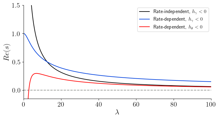
Figure 1: Results of the linear stability analysis for a rate-independent plastic model subject to internal softening (black line), for a rate-dependent plastic model subject to internal softening (blue line) and for a rate-dependent plastic model subject to coupling softening.

In this section, we will investigate the role of multiphysics coupling as a mean to regularize the strain localization problem. To put in perspective such role of the multiphysics coupling, we illustrate in Figure 1 the results obtained from linear stability analysis which emphasize the role of rate-dependency and multiphysics coupling. The solid black line corresponding to a rate-independent material subject to internal softening and no multiphysics coupling illustrate the ill-posedness of the strain localization problem for Cauchy continua. The rate of growth of the perturbation tends to infinity for zero wavelength characterizing a strain localization which is neither regularized in time nor in space. This leads to convergence problems for numerical simulators and mesh-sensitive strain localization results. As the dominant wavelength for strain localization is zero, deformation localizes in bands of the size of one element which prevents any reliable estimation of the localization thickness. The blue line, corresponding to a similar material but including rate-dependency (obtained by setting $h_{\gamma}<0$ and $h_{\theta}=0$ in Equation 13) illustrates the partial regularization of rate-dependent rheologies. The rate of growth of the perturbation reaches a bounded maximum for a zero wavelength. The viscous terms introduced by the rate-dependent constitutive laws allow to regularize the system in time (rate of growth does not tend towards infinity) but fail to regularize the strain localization problem in space as the regularization by rate dependence observed numerically disappears over time. It is thus only effective if used for loading timescales shorter than material relaxation time and the shear band size depends strongly on the imperfection wavelength imposed to trigger the localization. These findings have been covered in some details by Bažant & Jirásek [2002], Stefanou & Gerolymatou [2019]. The red solid line on the other hand corresponds to a rate-dependent material only subject to multiphysics coupling ($h_{\theta}<0$) without internal plastic hardening/softening ($h_{\gamma}=0$). Such setting allows to isolate the impact of multiphysics coupling on the strain localization regularization. The rate of growth of the perturbation reaches a maximum for a positive and bounded wavelength. The value of this wavelength (noted $\hat{\lambda}$) and corresponding to the maximum of the rate of growth of the perturbation allows to estimate the spatial extend of localized displacement or velocity fields or the spacing between regular patterns produced by strain localization.

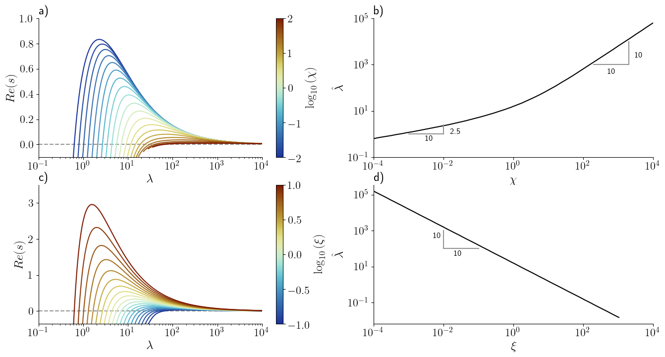
Figure 2: Impacts of diffusivity ratio $\chi$ and time scale ratio $\xi$ on the dominant wavelength of strain localization for a rate-dependent material subject to multiphysics softening only. Panels (a) and (c) show the results of the linear stability analysis for a range of values of $\chi$ and $\xi$ respectively. Panels (b) and (d) shows the dominant wavelength as a function of $\chi$ and $\xi$ respectively.

Figure 2 illustrates the dependency of the dominant wavelength $\hat{\lambda}$ on the physical parameters and boundary conditions of the problem for a material subject to multiphysics softening only. The impact of the diffusivity ratio $\chi$ (ratio of coupling diffusivity to momentum diffusivity) is illustrated in panels (a) and (b) in Figure 2. The dominant wavelength increases with the diffusivity ratio and a shift in the slope can be observed when the coupling diffusivity is greater than the momentum diffusivity (shift at $\chi\sim 1$). Below this critical value the diffusivity ratio is controlled by momentum diffusivity and the perturbation amplitude growths significantly faster (high values of $Re\left(s\right)$) than when the diffusivity ratio is dominated by the physical diffusivity of the coupled process. Panels (c) and (d) in Figure 2 illustrate the impact of the time scale ratio $\xi$ (ratio of the loading time scale to the viscous time scale). The dominant wavelength is inversely proportional to the time scale ratio (slope $-1$ in $\log$-$\log$ scale). Furthermore, for high values of the time scale ratio $\xi$ the perturbation grows significantly faster. This effect can be interpreted in terms of the loading conditions: for fast imposed strain rates, strain will localized slowly in a large extend whereas for slow imposed strain rates, strain will localized fast into small thicknesses. The findings presented here suggest that the introduction of viscous terms are not sufficient to regularize the strain localization problem (blue line in Figure 1). However, when considered together with a softening process controlled by a coupled diffused variable, strain localizes in finite thicknesses whose extents are physically controlled by the diffusivity and time scale ratios. As deforming solid materials are usually described with internal plastic hardening or softening, we investigate in the following the different regimes obtained when internal and multiphysics hardening/softening mechanisms interact or compete.

3.3 Combined multiphysics coupling and strain hardening/softening

In the following, we present the different responses of strain localization depending on the values of the parameters for a material undergoing both internal hardening/softening ($h_{\gamma}\neq 0$) and hardening/softening due to multiphysics coupling ($h_{\theta}\neq 0$).

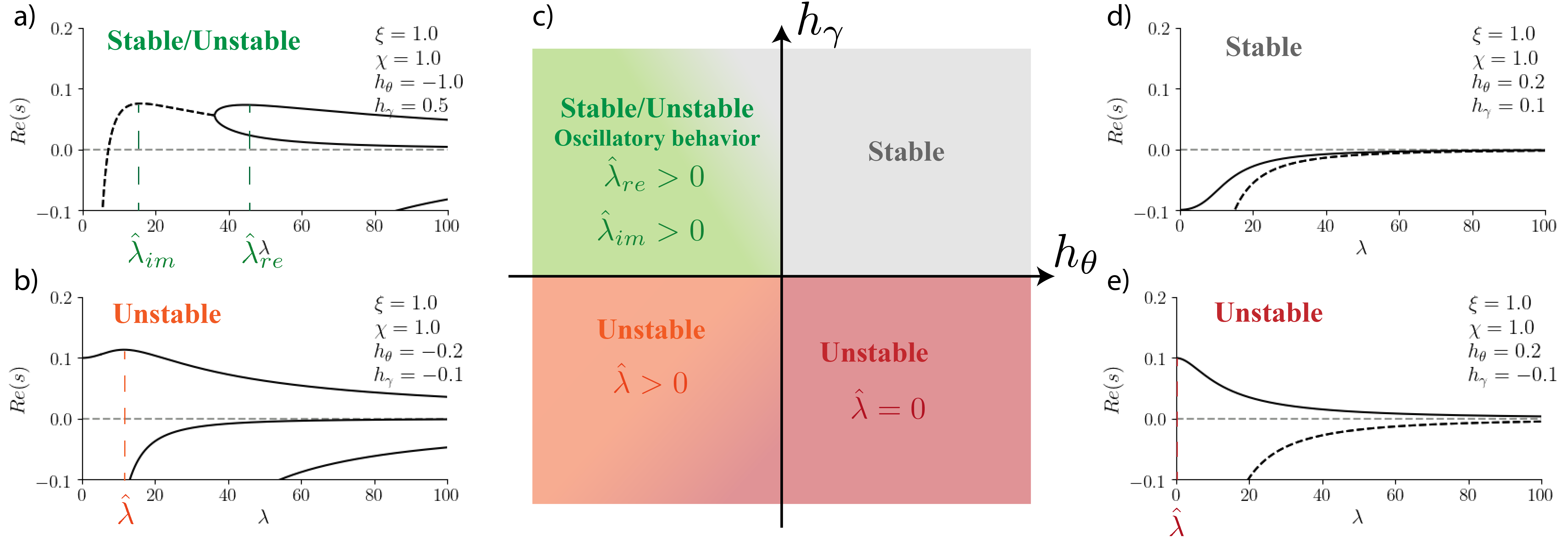
Figure 3: Overview of the results of the linear stability analysis. Panel (c) shows the stability conditions depending on the values of the two moduli $h_{\theta}$ and $h_{\gamma}$. Panels (a), (b), (d) and (e) show the real part of the rate of growth of the perturbation as a function of the perturbation wavelength for the representative regions described in panel (c). Solid lines indicate a pure real solution and dashed lines the real part of an imaginary solution. For each panel, we indicate the strain localization wavelength $\hat{\lambda}$ defined as the wavelength for which the rate of growth of the perturbation is maximum. The strain localization problem is said to be regularized if $0<\hat{\lambda}<+\infty$.

Figure 3 shows a map of the stability of the system depending on the values of the two plastic moduli $h_{\theta}$ and $h_{\gamma}$ together with representative linear stability analysis results for each case. If both moduli are positive, the material only undergoes hardening and the material behavior is always stable (gray region in panel (c) and panel (d)). If the material is subject to internal weakening and coupled hardening ($h_{\gamma}<0$ and $h_{\theta}>0$), the behavior is unconditionally unstable and a maximum bounded value of the real part of the rate of growth of the perturbation is obtained for a wavelength equals to zero (red region in panel (c) and panel (e)). Such system is characterized as being regularized in time because the maximum value of the rate of growth of the perturbation is bounded but remains unregularized in space as the dominant wavelength is zero. Similar results can be obtained in the case when $h_{\theta}=0$ and $h_{\gamma}<0$ as demonstrated by [Stefanou & Gerolymatou, 2019] and from the previous section (see Figure 1). When the material is subject to both internal weakening and coupled weakening ($h_{\gamma}<0$ and $h_{\theta}<0$, orange/red region in panel (c)), the system is unstable and can be regularized both in time and space as depicted in panel (b). We cover in this contribution the conditions necessary for regularizing the system in space, meaning that the dominant wavelength $\hat{\lambda}$ corresponding to the maximum of the rate of growth of the perturbation is finite and non-zero (see panel (b)). The last region, defined by competing internal hardening and coupled weakening ($h_{\theta}<0$ and $h_{\gamma}>0$, green region in panel (c) and panel (a)) give rise to a more complex behavior. Two local maxima of the real part of the rate of growth of the perturbation can be identified: one corresponding to a complex solution (dashed line in panel (a)) and a second one corresponding to a pure real solution (solid line). The existence of a complex unstable solution can be interpreted as an oscillatory instability. As the modulus $h_{\gamma}$ is increasing and the modulus $h_{\theta}$ tending toward zero, the real part of the rate of growth of the perturbation tends toward zero, hence exhibiting a continuous transition toward stable conditions (gray area in Figure 3-c). This regime is investigated in more details in section 5. In the following, we investigate the conditions for regularizing strain localization for a system characterized by internal and coupled weakening (panel (b)) and the underlying implications for the evolution of strain localization.

4 Strain localization regularization by standing waves ($h_{\gamma}<0$ and $h_{\theta}<0$)

In this section, we cover the regime described by a overall weakening both in the accumulated plastic strain ($h_{\gamma}<0$) and in the coupled variable ($h_{\theta}<0$). As depicted in Figure 3, this regime is unconditionally unstable but not necessarily regularized in a strain localization sense. We therefore describe under which conditions, both in terms of physical properties and boundary conditions, the strain localization phenomenon is regularized both in time and space.

4.1 Wavelength of strain localization

Figure 4 shows the results of the linear stability analysis for a regime characterized by softening both in plastic strain and in the coupled diffused variable depending on a range of values for the different physical parameters. We investigate the influence of the diffusivity ratio $\chi$, the time scale ratio $\xi$ and the two dimensionless plastic moduli $h_{\gamma}$ and $h_{\theta}$. For the given set of parameters, the results suggest that it exists a critical value of the diffusivity ratio for which the strain localization is regularized. For values of the diffusivity ratio ($\chi$) higher than this critical value, the maximum value for the rate of growth of the perturbation corresponds to a dimensionless wavelength of zero, meaning that the strain localization problem is ill-posed (see red line in Figure 4-a). The regularization of the strain localization problem by diffusive process occurs only for diffusivity ratios $\chi$ below this critical value (see blue line in Figure 4-a). In addition, decreasing the diffusivity ratio decreases the dominant wavelength of strain localization. The time scale ratio ($\xi$) does not have any impact on the regularization of the strain localization problem but only influence the absolute value of the rate of growth of the perturbation and its dominant wavelength. A low value of the time scale ratio $\xi$ corresponds to high viscous strain rates which leads to a fast growing perturbation. The effects of the plastic modulus $h_{\gamma}$ are similar to those of the effective strain rate ratio $\xi$. Increasing the plastic moduli however increases the value of the regularized wavelength. Finally the coupled plastic modulus $h_{\theta}$ influences the long wavelengths but has limited influences to short ones. Increasing the coupled plastic modulus leads to a decrease in the strain localization wavelength.

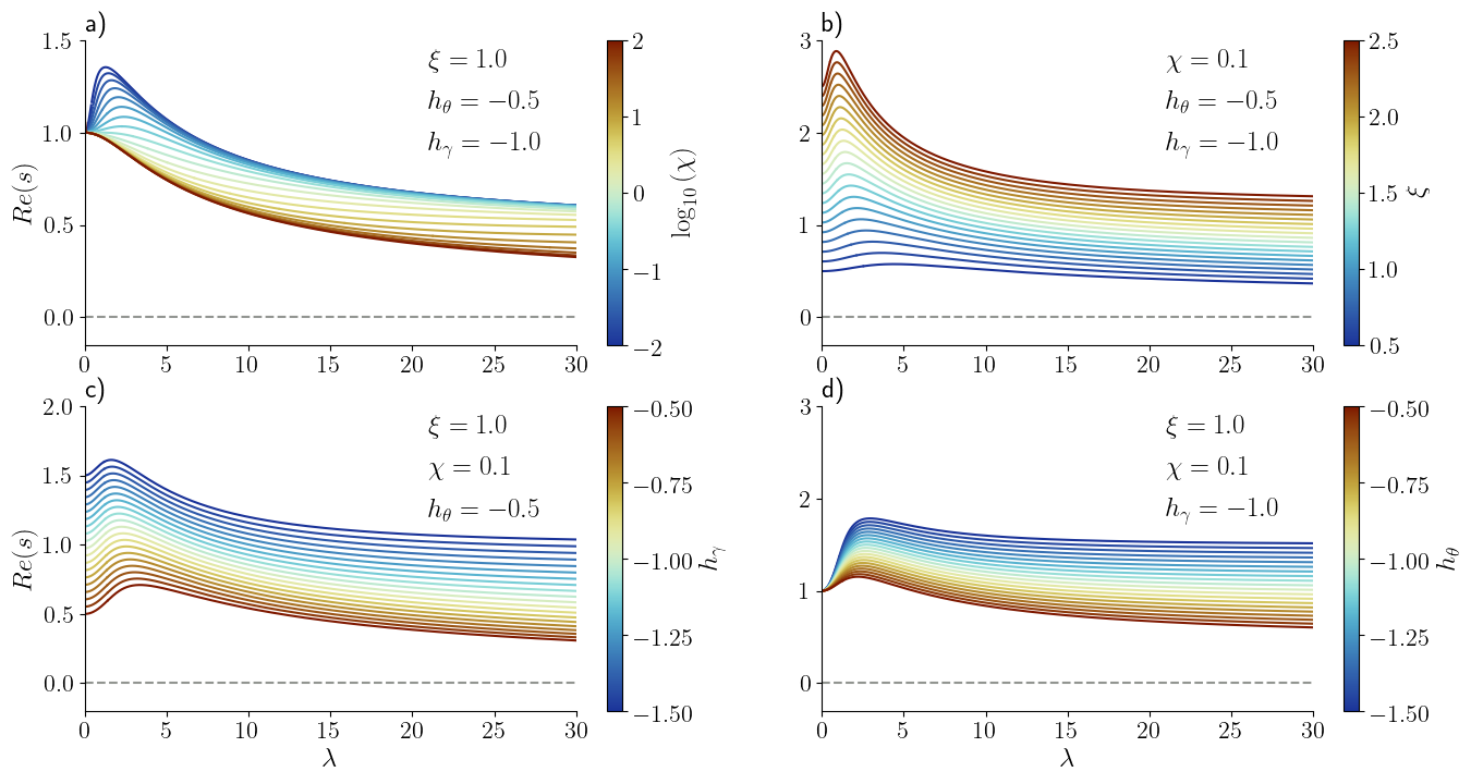
Figure 4: Results of the linear stability analysis in response to a range of values for the four physical parameters: diffusivity ratio $\chi$ (top left), time scale ratio $\xi$ (top right), internal plastic modulus $h_{\gamma}$ (bottom left) and plastic coupled modulus $h_{\theta}$ (bottom right).

Figure 5 illustrates the different regimes obtained by appropriately scaling all the parameters ($h_{\theta},h_{\gamma},\chi,\xi$) involved in the strain localization problem. We introduced the effective diffusivity ratio $\left|h_{\gamma}\right|\chi$ defined as the product of the diffusivity ratio and the absolute value of the internal weakening modulus and the effective coupled plastic modulus $\frac{1}{1+\left|h_{\theta}\right|}$ as a measure of the coupled weakening process. The regularization via diffusive process of the strain localization problem is only effective when the effective diffusivity ratio is smaller than one (see regime I in blue). For an overdiffused system, or for large internal weakening mechanism, the system is in general unregularized. In that case, for mild coupled weakening mechanism (low value of $h_{\theta}$), the strain localization wavelength tends toward zero (regime II in red) and for large coupled weakening mechanism (high value of $h_{\theta}$), it tends toward infinity (regime III in gray). A general condition for the regularization of the strain localization problem is therefore a low diffusivity of the internal diffusive process together with competing weakening mechanisms. In general, it can be concluded that internal weakening tends to unregularize the strain localization problem whereas coupled weakening favors an internal length scale. It is also worth noticing that our results suggest that the regime described in Figure 5 are independent from the time scale ratio $\xi$ and thus from the loading strain rate. However, this quantity impacts the obtained length scale of the strain localization as described in Figure 2.

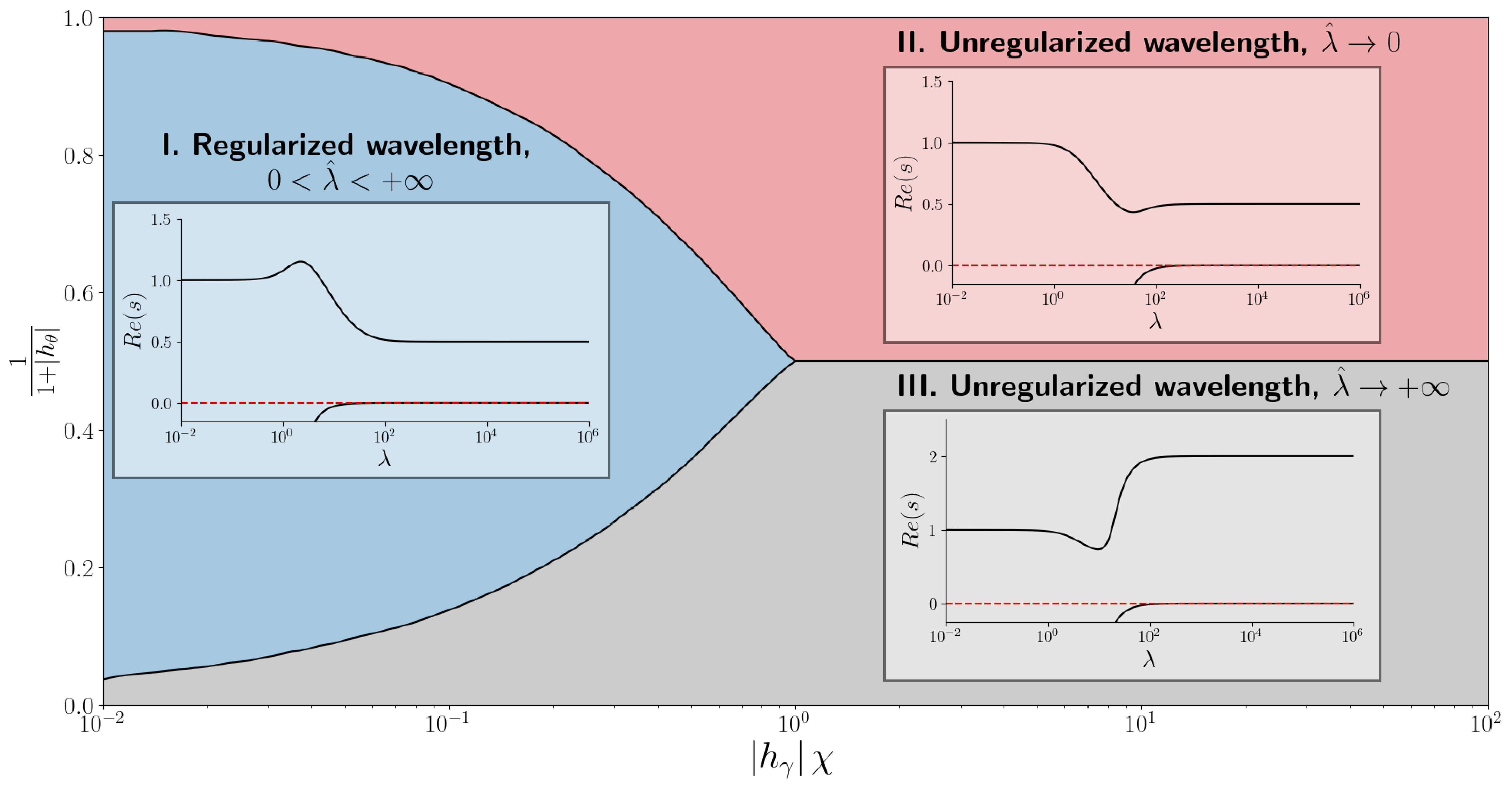
Figure 5: Phase diagram for the strain localization problem. The different regimes are displayed as a function of the effective diffusivity ratio $\left|h_{\gamma}\right|\chi$ and the effective coupled plastic modulus $\frac{1}{1+\left|h_{\theta}\right|}$. The blue regime refers to a regularized strain localization problem whereas the red and gray regimes refer to an unregularized problem for which the dominant wavelength either tends toward zero or infinity respectively.

4.2 Evolution of strain localization

To understand the implications of the existence of a regularized wavelength for strain localization, we performed dynamic simulations using the finite-element method. We implemented the system of equations described in Equation 13 relying on the MOOSE environment (Multiphysics Object-Oriented Simulation Environment) [Permann et al., 2020]. MOOSE is an open source environment for multiphysics Finite Element applications developed by the Idaho National Laboratories (INL, https://mooseframework.inl.gov/). It provides a flexible, hybrid parallel platform to solve for multiphysics and multicomponent problems in an implicit manner.

For this analysis, we consider a one-dimensional bar of dimensionless length $100$ subject to background strain rate $\dot{\gamma}_{0}$. As we are solving for the perturbations of the state variables, the displacement perturbation variable $\bar{u}^{\star}$ is initially homogeneous and equals to zero. The coupled variable perturbation $\theta^{\star}$ is initialized by considering a perturbation at the center of the domain given by the following equation:

$$\theta^{\star}\left(\bar{x},\bar{t}=0\right)=\begin{cases}\frac{1}{2}\theta^{\star}_{0}\left(1+\cos\left(\frac{2\pi\bar{x}}{\lambda_{0}}\right)\right),&\text{ if }-\frac{\lambda_{0}}{2}<\bar{x}<\frac{\lambda_{0}}{2},\\ 0&\text{otherwise.}\end{cases}$$ (18)

where $\theta^{\star}_{0}$ and $\lambda_{0}$ are the initial perturbation amplitude and wavelength respectively. The solution given by the finite-element analysis allows to describe the distribution and evolution with time of the displacement and coupled variable perturbation fields. We consider here the case where the physical parameters give a regularized wavelength as depicted for regime I in Figure 5.

Figure 6 shows the distribution and evolution in time of the strain rate perturbation for a regularized system. The initial perturbation in the coupled variable perturbation field drives the system to strain localization. The wavelength of the strain localization gradually evolves toward the value obtained from the linear stability analysis. As the initial wavelength of the perturbation is smaller than the internal wavelength of the system, the size of the strain localization increases progressively upon reaching the internal wavelength as depicted in Figure 7 showing the evolution of the strain localization wavelength with time. As the perturbation evolves over time, it generates regular patterns governed by the strain localization wavelength.

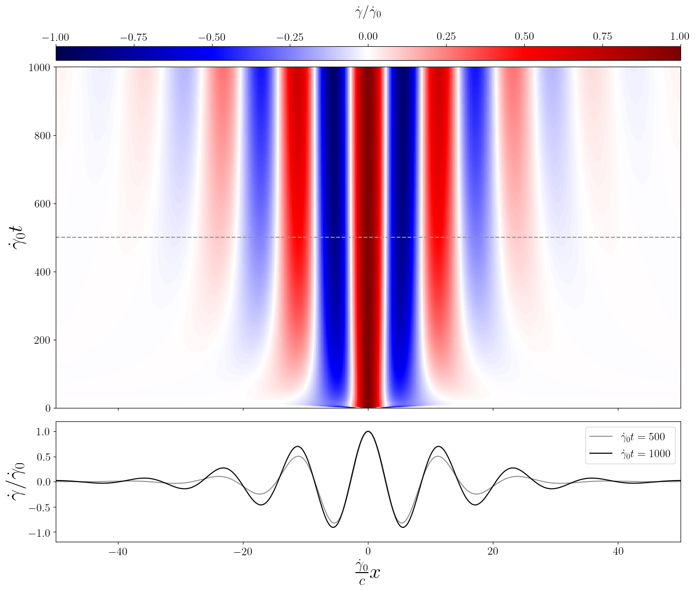
Figure 6: Evolution and distribution of the perturbation evaluated by finite-element analysis. The wavelength of the initial coupled variable perturbation is taken as $\lambda_{0}=5.0$. Top panel shows the distribution and evolution of the total strain rate. Bottom panel shows the distribution along the bar of the total strain rate at two different times. As the perturbations grows exponentially with time, normalized values are plotted.

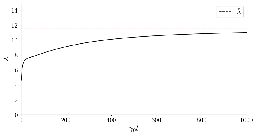
Figure 7: Evolution with time of the perturbation wavelength obtained from the finite-element simulations. The red dotted line indicates the dominant wavelength obtained from the linear stability analysis.

5 Strain localization regularization by standing and propagating waves ($h_{\gamma}>0$ and $h_{\theta}<0$)

In this section we investigate the case where deformation is characterized by competing hardening and softening. In particular, we consider the case where the system undergoes hardening in the plastic strain ($h_{\gamma}>0$) and softening in the coupled variable ($h_{\theta}<0$). As depicted in Figure 3 panel (a), this regime is characterized by two dominant wavelengths, the first one being attributed to standing waves and the second one to propagating waves. Here we investigate the conditions in terms of physical parameters and boundary conditions which allow these two sets of waves to interplay.

5.1 Standing and propagating waves

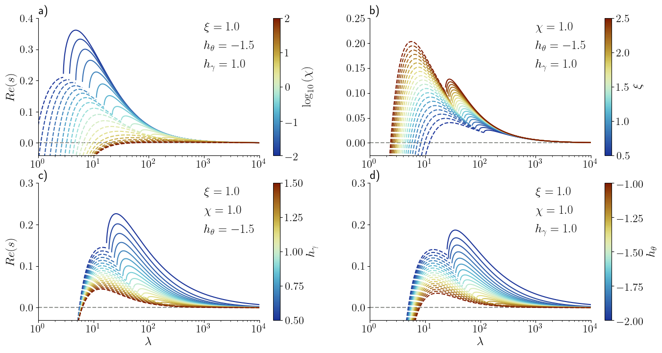
Figure 8: Results of the linear stability analysis in response to a range of values for the four physical parameters: diffusivity ratio $\chi$ (top left), time scale ratio $\xi$ (top right), internal plastic modulus $h_{\gamma}$ (bottom left) and plastic coupled modulus $h_{\theta}$ (bottom right).

Figure 8 illustrates the results of the linear stability analyses for a range of values of the four parameters ($\chi,\xi,h_{\gamma},h_{\theta}$). The perturbations evolve toward two different wavelengths upon strain localization as presented in Figure 8. The first one corresponds to an oscillatory regime (real part of a complex solution, dashed lines in Figure 8) which can be characterized by propagating waves. The second one (real solution, solid lines in Figure 8) corresponds to standing waves and is often referred as the spacing or the thickness of localized bands (see previous section and Figure 6). The coexistence of these two sets of waves highly depends on the parameter values which also dictate which regime dominates the strain localization phenomenon. An interesting aspect of these findings is that the diffusivity ratio $\chi$ seems to play a major role in switching between dominating standing waves (for low values of $\chi$) to dominating propagating waves (for high values of $\chi$) which captures the competing effect of physical to momentum diffusivities. The coupled diffusive process therefore controls how strain localization evolves in a deforming solid and the nature of its macroscopic manifestations. While the effect of the time scale ratio $\xi$ does not seem to influence the existence of standing and propagating waves, the diffusivity ratio $\chi$ and the two plastic moduli $h_{\gamma}$ and $h_{\theta}$ play a major role in controlling which waves (standing or propagating) are dominant. The competing effect of internal hardening and coupled softening is also relevant to the transition between the two regimes, which is well captured by the effective coupled plastic moduli $\frac{1}{1+\left|h_{\theta}\right|}$ bounded between zero and one and the effective diffusivity ratio $\left|h_{\gamma}\right|\chi$ as introduced in section 4.

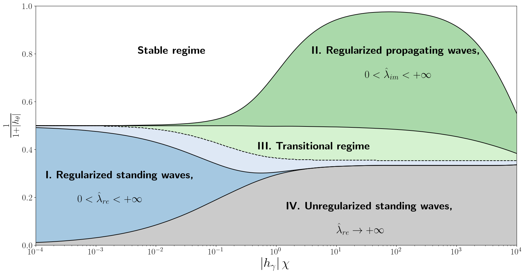
Figure 9: Phase diagram for the different strain localization regimes as a function of the effective diffusivity ratio $\left|h_{\gamma}\right|\chi$ and the effective coupled plastic modulus $\frac{1}{1+\left|h_{\theta}\right|}$. Regime I in blue corresponds to regularized standing waves, regime II in green to regularized propagating waves. Regime III is a transitional regime (light blue and light green) where the two wavelengths (standing and propagating waves) coexist. Light green region indicates that the propagating waves grow faster than the standing waves and the light blue region the opposite. Regime IV in gray indicates a non-regularized standing waves regime, similar to the gray regime in Figure 5. The white region indicates a stable behavior where the perturbations decrease over time.

Figure 9 illustrates the different regimes we identified in the $\left|h_{\gamma}\right|\chi$, $\frac{1}{1+\left|h_{\theta}\right|}$ space for a system undergoing internal hardening and coupled weakening. Standing waves are obtained when the coupled weakening mechanism dominates over the internal hardening mechanism and for low diffusivity ratio (high $h_{\theta}$ and low $\left|h_{\gamma}\right|\chi$). As the internal hardening or diffusivity increases, propagating waves can emerge, coexisting with the standing waves (transitional regime III as depicted in Figure 9). For low coupled weakening mechanism, standing waves can fade away and only propagating waves remain (regime II). For low coupled weakening mechanism at low effective diffusivity ratio, a stable regime is obtained where the perturbation fades away with time to go back to the steady-state solution. Similar to the findings presented in section 4, an unregularized standing waves regime is obtained for high coupled weakening mechanism leading to infinite wavelengths (regime IV in Figure 9).

5.2 Evolution of strain localization with interacting standing and propagating waves

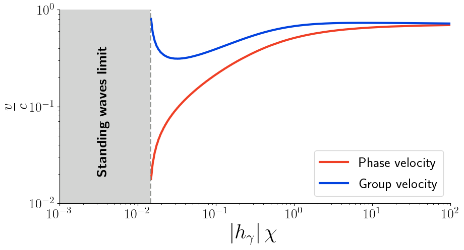
Figure 10: Evolution of the ratio of phase and group velocities to the elastic wave velocity as a function of the effective diffusivity ratio $\left|h_{\gamma}\right|\chi$ obtained with $h^{\theta}=-1.5$. Below a critical value of the effective diffusivity ratio, the standing waves regime is reached and the phase velocity tends toward zero and the group velocity toward infinity.

Figure 10 shows the evolution of the phase and group velocities (normalized by the elastic wave velocity) as a function of the effective diffusivity ratio $\left|h_{\gamma}\right|\chi$ as predicted by the linear stability analysis. Below a critical value of diffusivity, propagating waves vanish and the standing waves regime is reached. Approaching this regime, the group velocity tends toward infinity and the phase velocity to zero. The phase velocity is always lower than the group velocity but both converge to a constant value for high values of $\left|h_{\gamma}\right|\chi$. The strain localization waves velocity remains always smaller than the elastic wave velocity. These findings suggest that even in the case of propagating strain localization activated by diffusive process, the strain localization waves propagate slower than the elastic waves. In this case, the elastic wave velocity acts as a limit for strain localization propagation.

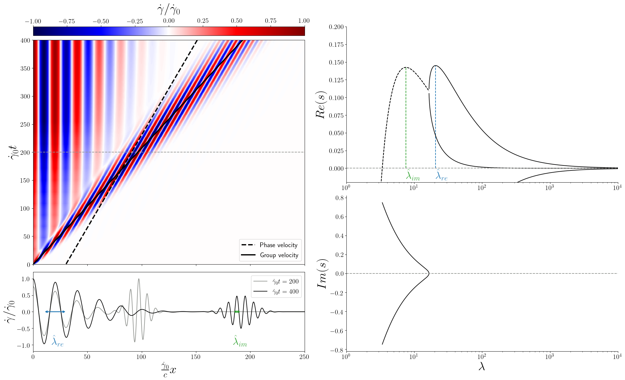
Figure 11: Left panels show the evolution and distribution of the normalized total strain rate for a dynamic simulation. The predicted phase and group velocities from the linear stability analysis are indicated as well as the two wavelengths corresponding to standing and propagating waves. Right panels show the results from the linear stability analysis for the set of parameters chosen in the dynamic simulation.

We performed some dynamic simulations for this regime using the finite-element-method based MOOSE framework Permann et al. [2020] to analyze the evolution of the strain localization. We cover the case of the standing waves regime in some details in section 4 and focus here on the transitional regime when both standing and propagating waves coexist. We consider a similar setting and the same initial perturbation in the coupled variable $\theta^{\star}$ (Equation 18) as presented in section 4 for a dimensionless bar of length $500$ centered in zero (we report here only the results of the positive half as the results are symmetric).

Figure 11 shows the distribution of the normalized total strain rate over time together with the results of the linear stability analysis for the system considered. The initial imposed perturbation generate a propagating wave characterized by a group velocity larger than the phase velocity as predicted by the linear stability analysis. Behind this propagating front, standing waves develop which self organize in a regular way. The two coexisting wavelengths predicted by the linear stability analysis match with the thickness of the standing and propagating waves. The macroscopic manifestation of such a transitional regime can be seen as an erratic distribution and propagation of deformation due to the discrepancy between phase and group velocities, followed by the formation of organized deformation patterns. The group and phase velocities observed in the simulations also match the predictions obtained from the linear stability analysis.

6 Discussion

In this study, we demonstrated under which conditions the introduction of a viscous term or the use of a viscoplastic model can successfully lead to the regularization of strain localization phenomena. The combination of viscoplasticity together with the multiphysics coupling to a diffusive process allows to carry the diffusive length scale to the deformation constitutive laws and therefore obtain a physical length scale for strain localization. The concept of viscous regularization has been widely studied in the modeling community. Several contributions investigated numerically the effect of viscoplasticity on the localization of the displacement or velocity fields with some success in terms of regularization of the ill-posed problem [Needleman, 1988, Loret & Prevost, 1990, Prevost & Loret, 1990, Duretz et al., 2014, 2019, Jacquey & Cacace, 2020] but always missed an analytical or mathematical proof that the length scale observed in the numerical results uprose from the constitutive laws. The results presented in this contribution argue that viscous terms alone do not regularize the strain localization in space but only in time. The artificial regularization observed in numerical models therefore is the results of a regularization in time from the viscous terms which allows to carry the length scale (usually quite large) introduced by the initial perturbation of the strain field. The length scale obtained in such models does not refer to a physical length scale but rather depends on the initial conditions, and thus on the size of the perturbation introduced. We report in this contribution that (i) viscous terms, (ii) inertia effects and (iii) multiphysics coupling are necessary to obtain a physical length scale for strain localization. Weakening mechanisms triggered by a coupled diffusive variable therefore tend to regularize the strain localization problem whereas internal weakening mechanisms promote unregularized internal length scale of zero size. The successful regularization of the strain localization problem, when the perturbation wavelength is positive, finite and determined by physical parameters depends on the competition between these two weakening mechanisms. While the loading rate conditions influence the size of the dominant wavelength and thus the internal length scale, they do not have any impact on the regularization conditions.

An essential aspect in the formulation we propose in this contribution is the coupling between the deformation mechanism and a diffusive process. This coupling allows to integrate the diffusive length-scale into the deformation localization phenomenon. As demonstrated in the present study, the dominant length-scale upon localization highly depends on the effective diffusivity of the material. This coupling is therefore essential to regularize the ill-posed problem of deformation localization. Such coupling is in general common for the rheological description of solid materials. Several studies considered thermo-mechanical [Veveakis et al., 2014a, Paesold et al., 2016] or chemo-mechanical [Brantut et al., 2011, Buscarnera, 2012, Stefanou & Sulem, 2014, Sulem & Stefanou, 2016] coupling as playing an important role for the regularization of strain localization. For geomaterials, generally described as porous media, the diffusion of pore pressure and saturation was also considered in the literature [Zhang & Schrefler, 2000, Schrefler et al., 2006, Veveakis & Regenauer-Lieb, 2015a, Alevizos et al., 2017, Oka et al., 2019]. The introduction of coupled diffusive process is also at the base of non-local theories such as gradient damage or breakage mechanics [Nguyen & Einav, 2010]. This study demonstrates how the coupling to a single diffusive process generates long-lasting localization patterns. Several studies considered the deformation of solid materials as the result of complex multiphysics involving several couplings to diffusive processes [Segall & Rice, 2006, Platt et al., 2014]. Such approaches, described as THMC (thermal-hydro-mechanical-chemical) coupling imply the existence of several length scales associated to the different diffusive processes considered [Veveakis & Regenauer-Lieb, 2015b]. The overall behavior of multiphysics solid materials can generally vary over the scale considered as each diffusive process is dominant at a specific length and time-scale. In this regard, the results presented in this contribution considering the coupling to a single diffusive process can be used to describe the multiphysics of deforming solid materials at a specific scale at which the chosen diffusive process is dominant. Extending the current approach to multiple diffusive processes, thus considering the multiscale aspect of the deformation of solid materials could be the topic of future studies.

We covered in this contribution two specific regimes which are characterized by the formation of regular patterns due to standing waves and by the formation of erratic patterns due to oscillatory solutions and the interplay of propagating and standing waves. As we solved for the dynamic evolution of a linearized system – we did not consider a particular form of the shear stress function but rather considered its derivatives evaluated at the steady-state solution – the patterns obtained are periodic in space and we could identify well-defined regimes. Considering a particular non-linear shear stress function would eventually not lead to similar periodic patterns as the derivative of the shear stress function are not constant over time in a general sense. This suggests that the deformation of a material characterized by a non-linear shear stress (which is generally the case) would not be limited to one of the particular regimes we described here but rather could evolve in time and therefore results in transient dominant wavelengths and a potential switch from erratic to regular pattern over time. In particular, most materials undergo hardening in the internal plastic strain after yielding and gradually transition to a softening regime upon continuous loading. Following the results presented here, this would imply that the dissipative propagating waves may emerge shortly after yielding but would vanish over time and let standing waves dominating the deformation at a larger time scale. The results we presented in this contribution could therefore have implications for the deformation of granular materials for which such waves have been observed in the laboratory [Guillard et al., 2015], for the initiation and propagation of earthquake rupture characterized by velocities lower than the elastic wave velocity [Kanamori, 1994], slow slip events [Dragert et al., 2001, Obara et al., 2004] or for the driving mechanisms responsible for the Portevin-Le Chatelier effect in steel and aluminum alloys which is characterized by the progressive formation of regular patterns [Yilmaz, 2016].

7 Conclusion

In this contribution, we investigate the behavior of a one-dimentional rate-dependent plastic formulation coupled to a diffusive process for deforming solid materials. We demonstrate the conditions in terms of physical parameters to regularize both in space and time strain localization using a linear stability analysis. We demonstrated that inertia effects together with the rate-dependency of the plasticity model adopted give minimum values for the applied strain rate and physical diffusivity values to effectively regularize the strain localization problem. Using finite-element analysis, we illustrated how the strain localization wavelength evolves over time in response to a given perturbation. The results described in this contribution are relevant to the multiscale description of localization phenomena in a large variety of solids exhibiting shear or compaction bands. As we considered a generic coupled diffusive process, the results presented in this contribution are extendable to any multiphysical system such as thermo-mechanical, chemo-mechanical or hydro-mechanical coupling but also to non-local theories such as gradient damage or breakage mechanics. We also investigated using the same set of governing equations, the existence of an oscillatory regime with two wavelengths with implications for the propagation of strain localization in the form of dissipative waves and the formation of erratic patterns.

References

- Alevizos et al. [2017] Alevizos, S., Poulet, T., Sari, M., Lesueur, M., Regenauer-Lieb, K., & Veveakis, M. (2017). A framework for fracture network formation in overpressurised impermeable shale: Deformability versus diagenesis. Rock Mechanics and Rock Engineering, 50, 689–703. URL: https://doi.org/10.1007/s00603-016-0996-y. doi:10.1007/s00603-016-0996-y.
- Antolovich & Armstrong [2014] Antolovich, S. D., & Armstrong, R. W. (2014). Plastic strain localization in metals: Origins and consequences. Progress in Materials Science, 59, 1–160. doi:10.1016/j.pmatsci.2013.06.001.
- Batra & Kim [1991] Batra, R., & Kim, C. (1991). Effect of thermal conductivity on the initiation, growth and bandwidth of adiabatic shear bands. International Journal of Engineering Science, 29, 949–960. doi:10.1016/0020-7225(91)90168-3.
- Baud et al. [2004] Baud, P., Klein, E., & fong Wong, T. (2004). Compaction localization in porous sandstones: Spatial evolution of damage and acoustic emission activity. Journal of Structural Geology, 26, 603–624. doi:10.1016/j.jsg.2003.09.002.
- Bažant & Jirásek [2002] Bažant, Z. P., & Jirásek, M. (2002). Nonlocal integral formulations of plasticity and damage: Survey of progress. Journal of Engineering Mechanics, 128, 1119–1149. doi:10.1061/(asce)0733-9399(2002)128:11(1119).
- Bayliss et al. [1994] Bayliss, A., Belytschko, T., Kulkarni, M., & Lott-Crumpler, D. A. (1994). On the dynamics and the role of imperfections for localization in thermo-viscoplastic materials. Modelling and Simulation in Materials Science and Engineering, 2, 941–964. doi:10.1088/0965-0393/2/5/001.
- Belytschko et al. [1991] Belytschko, T., Moran, B., & Kulkarni, M. (1991). On the crucial role of imperfections in quasi-static viscoplastic solutions. Journal of Applied Mechanics, 58, 658–665. doi:10.1115/1.2897246.
- Benallal [2005] Benallal, A. (2005). On localization modes in coupled thermo-hydro-mechanical problems. Comptes Rendus Mécanique, 333, 557–564. doi:10.1016/j.crme.2005.05.005.
- Benallal [2008] Benallal, A. (2008). A note on ill-posedness for rate-dependent problems and its relation to the rate-independent case. Computational Mechanics, 42, 261. doi:10.1007/s00466-008-0252-8.
- Benallal & Bigoni [2004] Benallal, A., & Bigoni, D. (2004). Effects of temperature and thermo-mechanical couplings on material instabilities and strain localization of inelastic materials. Journal of the Mechanics and Physics of Solids, 52, 725–753. doi:10.1016/s0022-5096(03)00118-2.
- Borst et al. [1993] Borst, R. D., Sluys, L., Muhlhaus, H., & Pamin, J. (1993). Fundamental issues in finite element analyses of localization of deformation. Engineering Computations, 10, 99–121. doi:10.1108/eb023897.
- Brantut et al. [2011] Brantut, N., Sulem, J., & Schubnel, A. (2011). Effect of dehydration reactions on earthquake nucleation: Stable sliding, slow transients, and unstable slip. Journal of Geophysical Research: Solid Earth, 116. URL: https://agupubs.onlinelibrary.wiley.com/doi/abs/10.1029/2010JB007876. doi:10.1029/2010JB007876.
- Budday et al. [2014] Budday, S., Steinmann, P., & Kuhl, E. (2014). The role of mechanics during brain development. Journal of the Mechanics and Physics of Solids, 72, 75–92. doi:10.1016/j.jmps.2014.07.010.
- Buscarnera [2012] Buscarnera, G. (2012). A conceptual model for the chemo-mechanical degradation of granular geomaterials. Géotechnique Letters, 2, 149–154. doi:10.1680/geolett.12.00020.
- Desrues et al. [1996] Desrues, J., Chambon, R., Mokni, M., & Mazerolle, F. (1996). Void ratio evolution inside shear bands in triaxial sand specimens studied by computed tomography. Geotechnique, 46, 529–546. doi:10.1680/geot.1996.46.3.529.
- Dragert et al. [2001] Dragert, H., Wang, K., & James, T. S. (2001). A silent slip event on the deeper cascadia subduction interface. Science, 292, 1525–1528. doi:10.1126/science.1060152.
- Duretz et al. [2019] Duretz, T., Borst, R., & Pourhiet, L. L. (2019). Finite thickness of shear bands in frictional viscoplasticity and implications for lithosphere dynamics. Geochemistry, Geophysics, Geosystems, 20, 5598–5616. doi:10.1029/2019gc008531.
- Duretz et al. [2014] Duretz, T., Schmalholz, S. M., Podladchikov, Y. Y., & Yuen, D. A. (2014). Physics‐controlled thickness of shear zones caused by viscous heating: Implications for crustal shear localization. Geophysical Research Letters, 41, 4904–4911. doi:10.1002/2014gl060438.
- Forest et al. [2005] Forest, S., Blazy, J. S., Chastel, Y., & Moussy, F. (2005). Continuum modeling of strain localization phenomena in metallic foams. Journal of Materials Science, 40, 5903–5910. doi:10.1007/s10853-005-5041-6.
- Fossen et al. [2007] Fossen, H., Schultz, R. A., Shipton, Z. K., & Mair, K. (2007). Deformation bands in sandstone: a review. Journal of the Geological Society, 164, 755–769. doi:10.1144/0016-76492006-036.
- Guillard et al. [2015] Guillard, F., Golshan, P., Shen, L., Valdes, J. R., & Einav, I. (2015). Dynamic patterns of compaction in brittle porous media. Nature Physics, 11, 835–838. doi:10.1038/nphys3424.
- Iordache & William [1998] Iordache, M.-M., & William, K. (1998). Localized failure analysis in elastoplastic Cosserat continua. Computer Methods in Applied Mechanics and Engineering, 151, 559–586. doi:10.1016/S0045-7825(97)00166-7.
- Issen & Rudnicki [2000] Issen, K. A., & Rudnicki, J. W. (2000). Conditions for compaction bands in porous rock. Journal of Geophysical Research: Solid Earth, 105, 21529. doi:10.1029/2000JB900185.
- Jacquey & Cacace [2020] Jacquey, A. B., & Cacace, M. (2020). Multiphysics modeling of a brittle‐ductile lithosphere: 1. explicit visco‐elasto‐plastic formulation and its numerical implementation. Journal of Geophysical Research: Solid Earth, 125. doi:10.1029/2019jb018474.
- Kamrin [2019] Kamrin, K. (2019). Non-locality in granular flow: Phenomenology and modeling approaches. Frontiers in Physics, 7, 116. URL: https://www.frontiersin.org/article/10.3389/fphy.2019.00116. doi:10.3389/fphy.2019.00116.
- Kanamori [1994] Kanamori, H. (1994). Mechanics of earthquakes. Annual Review of Earth and Planetary Sciences, 22, 207–237. doi:10.1146/annurev.ea.22.050194.001231.
- Loret & Prevost [1990] Loret, B., & Prevost, J. H. (1990). Dynamic strain localization in elasto-(visco-)plastic solids, Part 1. General formulation and one-dimensional examples. Computer Methods in Applied Mechanics and Engineering, 83, 247–273. doi:10.1016/0045-7825(90)90073-U.
- McAuliffe & Waisman [2013] McAuliffe, C., & Waisman, H. (2013). Mesh insensitive formulation for initiation and growth of shear bands using mixed finite elements. Computational Mechanics, 51, 807–823. doi:10.1007/s00466-012-0765-z.
- Molinari & Clifton [1987] Molinari, A., & Clifton, R. J. (1987). Analytical characterization of shear localization in thermoviscoplastic materials. Journal of Applied Mechanics, 54, 806–812. doi:10.1115/1.3173121.
- Molnár et al. [2018] Molnár, G., Rodney, D., Martoïa, F., Dumont, P. J., Nishiyama, Y., Mazeau, K., & Orgéas, L. (2018). Cellulose crystals plastify by localized shear. Proceedings of the National Academy of Sciences of the United States of America, 115, 7260–7265. doi:10.1073/pnas.1800098115.
- Mühlhaus & Vardoulakis [1987] Mühlhaus, H.-B., & Vardoulakis, I. (1987). The thickness of shear bands in granular materials. Géotechnique, 37, 271–283. doi:10.1680/geot.1987.37.3.271.
- Needleman [1988] Needleman, A. (1988). Material rate dependence and mesh sensitivity in localization problems. Computer Methods in Applied Mechanics and Engineering, 67, 69–85. doi:10.1016/0045-7825(88)90069-2.
- Nguyen & Einav [2010] Nguyen, G. D., & Einav, I. (2010). Nonlocal regularisation of a model based on breakage mechanics for granular materials. International Journal of Solids and Structures, 47, 1350 – 1360. URL: http://www.sciencedirect.com/science/article/pii/S0020768310000314. doi:10.1016/j.ijsolstr.2010.01.020.
- Obara et al. [2004] Obara, K., Hirose, H., Yamamizu, F., & Kasahara, K. (2004). Episodic slow slip events accompanied by non‐volcanic tremors in southwest japan subduction zone. Geophysical Research Letters, 31. doi:10.1029/2004gl020848.
- Oka et al. [2019] Oka, F., Shahbodagh, B., & Kimoto, S. (2019). A computational model for dynamic strain localization in unsaturated elasto-viscoplastic soils. International Journal for Numerical and Analytical Methods in Geomechanics, 43, 138–165. URL: https://onlinelibrary.wiley.com/doi/abs/10.1002/nag.2857. doi:10.1002/nag.2857.
- Paesold et al. [2016] Paesold, M. K., Bassom, A. P., Regenauer-Lieb, K., & Veveakis, M. (2016). Conditions for the localisation of plastic deformation in temperature sensitive viscoplastic materials. Journal of Mechanics and Materials and Structures, 11, 113 – 136. URL: https://msp.org/jomms/2016/11-2/p02.xhtml. doi:10.2140/jomms.2016.11.113.
- Permann et al. [2020] Permann, C. J., Gaston, D. R., Andrš, D., Carlsen, R. W., Kong, F., Lindsay, A. D., Miller, J. M., Peterson, J. W., Slaughter, A. E., Stogner, R. H., & Martineau, R. C. (2020). MOOSE: Enabling massively parallel multiphysics simulation. SoftwareX, 11, 100430. URL: http://www.sciencedirect.com/science/article/pii/S2352711019302973. doi:https://doi.org/10.1016/j.softx.2020.100430.
- Pijaudier-Cabot & Bazant [1987] Pijaudier-Cabot, G., & Bazant, Z. P. (1987). Non local Damage Theory. Journal of engineering mechanics, 113, 1512–1533. doi:http://dx.doi.org/10.1061/(ASCE)0733-9399(1987)113:10(1512).
- Platt et al. [2014] Platt, J. D., Rudnicki, J. W., & Rice, J. R. (2014). Stability and localization of rapid shear in fluid‐saturated fault gouge: 2. Localized zone width and strength evolution. Journal of Geophysical Research: Solid Earth, 119, 4334–4359. doi:10.1002/2013jb010711.
- Prevost & Loret [1990] Prevost, J. H., & Loret, B. (1990). Dynamic strain localization in elasto-(visco-)plastic solids, part 2. plane strain examples. Computer Methods in Applied Mechanics and Engineering, 83, 275–294. doi:10.1016/0045-7825(90)90074-v.
- Rattez et al. [2018a] Rattez, H., Stefanou, I., & Sulem, J. (2018a). The importance of Thermo-Hydro-Mechanical couplings and microstructure to strain localization in 3D continua with application to seismic faults. Part I: Theory and linear stability analysis. Journal of the Mechanics and Physics of Solids, 115, 54–76. doi:10.1016/j.jmps.2018.03.004.
- Rattez et al. [2018b] Rattez, H., Stefanou, I., Sulem, J., Veveakis, M., & Poulet, T. (2018b). The importance of Thermo-Hydro-Mechanical couplings and microstructure to strain localization in 3D continua with application to seismic faults . Part II : Numerical implementation and post-bifurcation analysis. Journal of the Mechanics and Physics of Solids, 115, 1–29. doi:10.1016/j.jmps.2018.03.003.
- Rice et al. [2014] Rice, J. R., Rudnicki, J. W., & Platt, J. D. (2014). Stability and localization of rapid shear in fluid-saturated fault gouge : 1 . Linearized stability analysis. Journal of Geophysical Research, (pp. 1–23). doi:10.1002/2013JB010710.Received.
- Richman et al. [1975] Richman, D. P., Sturat, R. M., Hutchinson, J. W., & Caviness, V. S. J. (1975). Mechanical model of brain convolutional development. Science, 189, 18–21. doi:10.1126/science.1135626.
- Rudnicki & Rice [1975] Rudnicki, J. W., & Rice, J. R. (1975). Conditions for the localization of deformation in pressure-sensitive dilatant materials. Journal of the Mechanics and Physics of Solids, 23, 371–394. doi:10.1016/0022-5096(75)90001-0.
- Schrefler et al. [2006] Schrefler, B., Zhang, H., & Sanavia, L. (2006). Interaction between different internal length scales in strain localization analysis of fully and partially saturated porous media—the 1-d case. International Journal for Numerical and Analytical Methods in Geomechanics, 30, 45–70. doi:10.1002/nag.474.
- Segall & Rice [2006] Segall, P., & Rice, J. R. (2006). Does shear heating of pore fluid contribute to earthquake nucleation? Journal of Geophysical Research: Solid Earth (1978–2012), 111. doi:10.1029/2005JB004129.
- Stefanou & Gerolymatou [2019] Stefanou, I., & Gerolymatou, E. (2019). Strain localization in geomaterials and regularization: rate-dependency, higher order continuum theories and multi-physics. In J. Sulem, & C. Viggiani (Eds.), ALERT Doctoral School 2019: The legacy of Ioannis Vardoulakis to Geomechanics chapter 3. (pp. 47–85).
- Stefanou & Sulem [2014] Stefanou, I., & Sulem, J. (2014). Chemically induced compaction bands: Triggering conditions and band thickness. Journal of Geophysical Research: Solid Earth, 119, 880–899. URL: https://agupubs.onlinelibrary.wiley.com/doi/abs/10.1002/2013JB010342. doi:10.1002/2013JB010342.
- Sulem & Stefanou [2016] Sulem, J., & Stefanou, I. (2016). Thermal and chemical effects in shear and compaction bands. Geomechanics for Energy and the Environment, 6, 4 – 21. doi:https://doi.org/10.1016/j.gete.2015.12.004.
- Tresca [1878] Tresca, M. (1878). On further applications of the flow of solids. Journal of the Franklin Institute, 106, 396–404. doi:10.1016/0016-0032(78)90047-9.
- Vardoulakis & Aifantis [1991] Vardoulakis, I., & Aifantis, E. C. (1991). A gradient flow theory of plasticity for granular materials. Acta Mechanica, 87, 197–217.
- Vardoulakis & Sulem [1995] Vardoulakis, I., & Sulem, J. (1995). Bifurcation Analysis in Geomechanics. Glascow: Blackie.
- Veveakis & Regenauer-Lieb [2015a] Veveakis, E., & Regenauer-Lieb, K. (2015a). Cnoidal waves in solids. Journal of the Mechanics and Physics of Solids, 78, 231 – 248. URL: http://www.sciencedirect.com/science/article/pii/S0022509615000411. doi:10.1016/j.jmps.2015.02.010.
- Veveakis & Regenauer-Lieb [2015b] Veveakis, E., & Regenauer-Lieb, K. (2015b). Review of extremum postulates. Current Opinion in Chemical Engineering, 7, 40 – 46. URL: http://www.sciencedirect.com/science/article/pii/S2211339814000860. doi:https://doi.org/10.1016/j.coche.2014.10.006.
- Veveakis et al. [2014a] Veveakis, E., Regenauer-Lieb, K., & Weinberg, R. (2014a). Ductile compaction of partially molten rocks: the effect of non-linear viscous rheology on instability and segregation. Geophysical Journal International, 200, 519–523. URL: https://doi.org/10.1093/gji/ggu412. doi:10.1093/gji/ggu412.
- Veveakis et al. [2014b] Veveakis, M., Poulet, T., & Alevizos, S. (2014b). Thermo-poro-mechanics of chemically active creeping faults: 2. Transient considerations. Journal of Geophysical Research: Solid Earth, 119, 4583–4605. doi:10.1002/2013JB010071.
- Wang et al. [1996] Wang, W., Sluys, L., & de Borst, R. (1996). Interaction between material length scale and imperfection size for localisation phenomena in viscoplastic media. European Journal of Mechanics - A/Solids, 15, 447–464.
- Yilmaz [2016] Yilmaz, A. (2016). The portevin–le chatelier effect: a review of experimental findings. Science and Technology of Advanced Materials, 12, 063001. doi:10.1088/1468-6996/12/6/063001.
- Zhang & Schrefler [2000] Zhang, H. W., & Schrefler, B. A. (2000). Gradient-dependent plasticity model and dynamic strain localisation analysis of saturated and partially saturated porous media: one dimensional model. European Journal of Mechanics - A/Solids, 19, 503 – 524. doi:https://doi.org/10.1016/S0997-7538(00)00177-7.