Near-Optimal Data Source Selection for Bayesian Learning

Abstract

We study a fundamental problem in Bayesian learning, where the goal is to select a set of data sources with minimum cost while achieving a certain learning performance based on the data streams provided by the selected data sources. First, we show that the data source selection problem for Bayesian learning is NP-hard. We then show that the data source selection problem can be transformed into an instance of the submodular set covering problem studied in the literature, and provide a standard greedy algorithm to solve the data source selection problem with provable performance guarantees. Next, we propose a fast greedy algorithm that improves the running times of the standard greedy algorithm, while achieving performance guarantees that are comparable to those of the standard greedy algorithm. The fast greedy algorithm can also be applied to solve the general submodular set covering problem with performance guarantees. Finally, we validate the theoretical results using numerical examples, and show that the greedy algorithms work well in practice.

Keywords: Bayesian Learning, Combinatorial Optimization, Approximation Algorithms, Greedy Algorithms

1 Introduction

The problem of learning the true state of the world based on streams of data has been studied by researchers from different fields. A classical method to tackle this task is Bayesian learning, where we start with a prior belief about the true state of the world and update our belief based on the data streams from the data sources (e.g., [8]). In particular, the data streams can come from a variety of sources, including experiment outcomes [3], medical tests [13], and sensor measurements [15], etc. In practice, we need to pay a cost in order to obtain the data streams from the data sources; for example, conducting certain experiments or installing a particular sensor incurs some cost that depends on the nature of the corresponding data source. Thus, a fundamental problem that arises in Bayesian learning is to select a subset of data sources with the smallest total cost, while ensuring a certain level of the learning performance based on the data streams provided by the selected data sources.

In this paper, we focus on a standard Bayesian learning rule that updates the belief on the true state of the world recursively based on the data streams. The learning performance is then characterized by an error given by the difference between the steady-state belief obtained from the learning rule and the true state of the world. Moreover, we consider the scenario where the data sources are selected a priori before running the Bayesian learning rule, and the set of selected data sources is fixed over time. We then formulate and study the Bayesian Learning Data Source Selection (BLDS) problem, where the goal is to minimize the cost spent on the selected data sources while ensuring that the error of the learning process is within a prescribed range.

1.1 Related Work

In [5] and [9], the authors studied the data source selection problem for Bayesian active learning. They considered the scenario where the data sources are selected in a sequential manner with a single data source selected at each time step in the learning process. The goal is then to find a policy on sequentially selecting the data sources with minimum cost, while the true state of the world can be identified based on the selected data sources. In contrast, we consider the scenario where a subset of data sources are selected a priori. Moreover, the selected data sources may not necessarily lead to the learning of the true state of the world. Thus, we characterize the performance of the learning process via its steady-state error.

The problem studied in this paper is also related but different from the problem of ensuring sparsity in learning, where the goal is to identify the fewest number of features in order to explain a given set of data [22, 14].

Finally, our problem formulation is also related to the sensor placement problem that has been studied for control systems (e.g., [19] and [25]), signal processing (e.g., [4] and [24]), and machine learning (e.g., [15]). In general, the goal of these problems is either to optimize certain (problem-specific) performance metrics of the estimate associated with the measurements of the placed sensors while satisfying the sensor placement budget constraint, or to minimize the cost spent on the placed sensors while ensuring that the estimation performance is within a certain range.

1.2 Contributions

First, we formulate the Bayesian Learning Data Source Selection (BLDS) problem, and show that the BLDS problem is NP-hard. Next, we show that the BLDS problem can be transformed into an instance of the submodular set covering problem studied in [23]. The BLDS problem can then be solved using a standard greedy algorithm with approximation (i.e., performance) guarantees, where the query complexity of the greedy algorithm is $O(n^{2})$, with $n$ to be the number of all candidate data sources. In order to improve the running times of the greedy algorithm, we further propose a fast greedy algorithm with query complexity $O(\frac{n}{\epsilon}\ln\frac{n}{\epsilon})$, where $\epsilon\in(0,1)$. The fast greedy algorithm achieves comparable performance guarantees to those of the standard greedy algorithm, and can also be applied to solve the general submodular set covering problem with performance guarantees. Finally, we provide illustrative examples to interpret the performance bounds obtained for the greedy algorithms applied to the BLDS problem, and give simulation results.

1.3 Notation and Terminology

The sets of integers and real numbers are denoted as $\mathbb{Z}$ and $\mathbb{R}$, respectively. For a vector $x\in\mathbb{R}^{n}$, we denote its transpose as $x^{\prime}$. For $x\in\mathbb{R}$, let $\lceil x\rceil$ be the smallest integer that is greater than or equal to $x$. Given any integer $n\geq 1$, we define $[n]\triangleq\{1,\dots,n\}$. The cardinality of a set $\mathcal{A}$ is denoted by $|\mathcal{A}|$. Given two functions $\varphi_{1}:\mathbb{R}_{\geq 0}\to\mathbb{R}$ and $\varphi_{2}:\mathbb{R}_{\geq 0}\to\mathbb{R}$, $\varphi_{1}(n)$ is $O(\varphi_{2}(n))$ if there exist positive constants $c$ and $N$ such that $|\varphi_{1}(n)|\leq c|\varphi_{2}(n)|$ for all $n\geq N$.

2 The Bayesian Learning Data Source Selection Problem

In this section, we formulate the data source selection problem for Bayesian learning that we will study in this paper. Let $\Theta\triangleq\{\theta_{1},\theta_{2},\dots,\theta_{m}\}$ be a finite set of possible states of the world, where $m\triangleq|\Theta|$. We consider a set $[n]$ of data sources that can provide data streams of the state of the world. At each discrete time step $k\in\mathbb{Z}_{\geq 1}$, the signal (or observation) provided by source $i\in[n]$ is denoted as $\omega_{i,k}\in S_{i}$, where $S_{i}$ is the signal space of source $i$. Conditional on the state of the world $\theta\in\Theta$, an observation profile of the $n$ sources at time $k$, denoted as $\omega_{k}\triangleq(\omega_{1,k},\dots,\omega_{n,k})\in S_{1}\times\cdots\times S_{n}$, is generated by the likelihood function $\ell(\cdot|\theta)$. Let $\ell_{i}(\cdot|\theta)$ denote the $i$-th marginal of $\ell(\cdot|\theta)$, which is the signal structure of data source $i\in[n]$. We make the following assumption on the observation model (e.g., see [10, 17, 16, 20]).

Assumption 1.

For each source $i\in[n]$, the signal space $S_{i}$ is finite, and the likelihood function $\ell_{i}(\cdot|\theta)$ satisfies $l_{i}(s_{i}|\theta)>0$ for all $s_{i}\in S_{i}$ and for all $\theta\in\Theta$. Furthermore, for all $\theta\in\Theta$, the observations are independent over time, i.e., $\{\omega_{i,1},\omega_{i,2},\dots\}$ is a sequence of independent identically distributed (i.i.d.) random variables. The likelihood function is assumed to satisfy $\ell(\cdot|\theta)=\prod_{i=1}^{n}\ell_{i}(\cdot|\theta)$ for all $\theta\in\Theta$, where $\ell_{i}(\cdot|\theta)$ is the $i$-th marginal of $\ell(\cdot|\theta)$.

Consider the scenario where there is a (central) designer who needs to select a subset of data sources in order to learn the true state of the world based on the observations from the selected sources. Specifically, each data source $i\in[n]$ is assumed to have an associated selection cost $h_{i}\in\mathbb{R}_{>0}$. Considering any $\mathcal{I}\triangleq\{n_{1},n_{2},\dots,n_{\tau}\}$ with $\tau=|\mathcal{I}|$, we let $h(\mathcal{I})$ denote the sum of the costs of the selected sources in $\mathcal{I}$, i.e., $h(\mathcal{I})\triangleq\sum_{n_{i}\in\mathcal{I}}h_{n_{i}}$. Let $\omega_{\mathcal{I},k}\triangleq(\omega_{n_{1},k},\dots,\omega_{n_{\tau},k})\in S_{n_{1}}\times\cdots\times S_{n_{\tau}}$ be the observation profile (conditioned on $\theta\in\Theta$) generated by the likelihood function $\ell_{\mathcal{I}}(\cdot|\theta)$, where $\ell_{\mathcal{I}}(\cdot|\theta)=\prod_{i=1}^{\tau}\ell_{n_{i}}(\cdot|\theta)$. We assume that the designer knows $\ell_{i}(\cdot|\theta)$ for all $\theta\in\Theta$ and for all $i\in[n]$, and thus knows $\ell_{\mathcal{I}}(\cdot|\theta)$ for all $\mathcal{I}\subseteq[n]$ and for all $\theta\in\Theta$. After the data sources are selected, the designer updates its belief of the state of the world using the following standard Bayes’ rule:

$$\mu^{\mathcal{I}}_{k+1}(\theta)=\frac{\mu_{0}(\theta)\prod_{j=0}^{k}\ell_{\mathcal{I}}(\omega_{\mathcal{I},j+1}|\theta)}{\sum_{\theta_{p}\in\Theta}\mu_{0}(\theta_{p})\prod_{j=0}^{k}\ell_{\mathcal{I}}(\omega_{\mathcal{I},j+1}|\theta_{p})}\ \forall\theta\in\Theta,$$ (1)

where $u^{\mathcal{I}}_{k+1}(\theta)$ is the belief of the designer that $\theta$ is the true state at time step $k+1$, and $\mu_{0}(\theta)$ is the initial (or prior) belief of the designer that $\theta$ is the true state. We take $\sum_{\theta\in\Theta}\mu_{0}(\theta)=1$ and $\mu_{0}(\theta)\in\mathbb{R}_{\geq 0}$ for all $\theta\in\Theta$. Note that $\sum_{\theta\in\Theta}\mu^{\mathcal{I}}_{k}(\theta)=1$ for all $\mathcal{I}\subseteq[n]$ and for all $k\in\mathbb{Z}_{\geq 1}$, where $0\leq\mu_{k}^{\mathcal{I}}(\theta)\leq 1$ for all $\theta\in\Theta$. In other words, $\mu_{k}^{\mathcal{I}}(\cdot)$ is a probability distribution over $\Theta$ for all $k\in\mathbb{Z}_{\geq 1}$ and for all $\mathcal{I}\subseteq[n]$. Rule (1) is also equivalent to the following recursive rule:

$$\mu^{\mathcal{I}}_{k+1}(\theta)=\frac{\mu^{\mathcal{I}}_{k}(\theta)\ell_{\mathcal{I}}(\omega_{\mathcal{I},k+1}|\theta)}{\sum_{\theta_{p}\in\Theta}\mu^{\mathcal{I}}_{k}(\theta_{p})\ell_{\mathcal{I}}(\omega_{\mathcal{I},k+1}|\theta_{p})}\ \forall\theta\in\Theta,$$ (2)

with $\mu_{0}^{\mathcal{I}}(\theta)\triangleq\mu_{0}(\theta)$ for all $\mathcal{I}\subseteq[n]$. For a given state $\theta\in\Theta$ and a given $\mathcal{I}\subseteq[n]$, we define the set of observationally equivalent states to $\theta$ as

$$F_{\theta}(\mathcal{I})\triangleq\mathop{\arg\min}_{\theta_{p}\in\Theta}D_{KL}(\ell_{\mathcal{I}}(\cdot|\theta_{p})\|\ell_{\mathcal{I}}(\cdot|\theta)),$$ (3)

where $D_{KL}(\ell_{\mathcal{I}}(\cdot|\theta_{p})\|\ell_{\mathcal{I}}(\cdot|\theta))$ is the Kullback-Leibler (KL) divergence between the likelihood functions $\ell_{\mathcal{I}}(\cdot|\theta_{p})$ and $\ell_{\mathcal{I}}(\cdot|\theta)$. Noting that $D_{KL}(\ell_{\mathcal{I}}(\cdot|\theta)\|\ell_{\mathcal{I}}(\cdot|\theta))=0$ and that the KL divergence is always nonnegative, we have $\theta\in F_{\theta}(\mathcal{I})$ for all $\theta\in\Theta$ and for all $\mathcal{I}\subseteq[n]$. Equivalently, we can write $F_{\theta}(\mathcal{I})$ as

$$F_{\theta}(\mathcal{I})=\{\theta_{p}\in\Theta:\ \ell_{\mathcal{I}}(s_{\mathcal{I}}|\theta_{p})=\ell_{\mathcal{I}}(s_{\mathcal{I}}|\theta),\forall s_{\mathcal{I}}\in S_{\mathcal{I}}\},$$ (4)

where $S_{\mathcal{I}}\triangleq S_{n_{1}}\times\cdots\times S_{n_{\tau}}$. Note that $F_{\theta}(\mathcal{I})$ is the set of states that cannot be distinguished from $\theta$ based on the data streams provided by the data sources indicated by $\mathcal{I}$. Moreover, we define $F_{\theta}(\emptyset)\triangleq\Theta$. Noting that $\ell_{\mathcal{I}}(\cdot|\theta)=\prod_{i=1}^{\tau}\ell_{n_{i}}(\cdot|\theta)$ under Assumption 1, we can further obtain from Eqs. (3)-(4) the following:

$$F_{\theta}(\mathcal{I})=\bigcap_{n_{i}\in\mathcal{I}}F_{\theta}(n_{i}),$$ (5)

for all $\mathcal{I}\subseteq[n]$ and for all $\theta\in\Theta$. Using similar arguments to those for Lemma $1$ in [18], one can show the following result.

Lemma 1.

Suppose the true state of the world is $\theta^{*}$, and $\mu_{0}(\theta)>0$ for all $\theta\in\Theta$. For all $\mathcal{I}\subseteq[n]$, the rule given in (1) ensures: (a) $\mathop{\lim}_{k\to\infty}\mu^{\mathcal{I}}_{k}(\theta_{p})=0$ almost surely (a.s.) for all $\theta_{p}\notin F_{\theta^{*}}(\mathcal{I})$; and (b) $\lim_{k\to\infty}\mu^{\mathcal{I}}_{k}(\theta_{q})=\frac{\mu_{0}(\theta_{q})}{\sum_{\theta\in F_{\theta^{*}}(\mathcal{I})}\mu_{0}(\theta)}$ a.s. for all $\theta_{q}\in\ F_{\theta^{*}}(\mathcal{I})$, where $F_{\theta^{*}}(\mathcal{I})$ is given by Eq. (5).

Consider a true state $\theta^{*}\in\Theta$ and a set $\mathcal{I}\subseteq[n]$ of selected sources. In order to characterize the (steady-state) learning performance of rule (1), we will use the following error metric (e.g., [11]):

$$e_{\theta^{*}}(\mathcal{I})\triangleq\frac{1}{2}\mathop{\lim}_{k\to\infty}\|\mu^{\mathcal{I}}_{k}-\mathbf{1}_{\theta^{*}}\|_{1},$$ (6)

where $\mu^{\mathcal{I}}_{k}\triangleq\begin{bmatrix}\mu^{\mathcal{I}}_{k}(\theta_{1})&\cdots&\mu^{\mathcal{I}}_{k}(\theta_{m})\end{bmatrix}^{\prime}$, and $\mathbf{1}_{\theta^{*}}\in\mathbb{R}^{m}$ is a (column) vector where the element that corresponds to $\theta^{*}$ is $1$ and all the other elements are zero. Note that $\frac{1}{2}\|\mu^{\mathcal{I}}_{k}-\mathbf{1}_{\theta^{*}}\|_{1}$ is also known as the total variation distance between the two distributions $\mu_{k}^{\mathcal{I}}$ and $\mathbf{1}_{\theta^{*}}$ (e.g., [2]). Also note that $e_{\theta^{*}}(\mathcal{I})$ exists (a.s.) due to Lemma 1. We then see from Lemma 1 that $e_{\theta^{*}}(\mathcal{I})=1-\frac{\mu_{0}(\theta^{*})}{\sum_{\theta\in F_{\theta^{*}}(\mathcal{I})}\mu_{0}(\theta)}$ holds almost surely. Since the true state is not known a priori to the designer, we further define

$$e^{s}_{\theta_{p}}(\mathcal{I})\triangleq 1-\frac{\mu_{0}(\theta_{p})}{\sum_{\theta\in F_{\theta_{p}}(\mathcal{I})}\mu_{0}(\theta)}\ \forall\theta_{p}\in\Theta,$$ (7)

which represents the (steady-state) total variation distance between the designer’s belief $\mu_{k}^{\mathcal{I}}$ and $\mathbf{1}_{\theta_{p}}$, when $\theta_{p}$ is assumed to be the true state of the world. We then define the Bayesian Learning Data Source Selection (BLDS) problem as follows.

Problem 1.

(BLDS) Consider a set $\Theta=\{\theta_{1},\dots,\theta_{m}\}$ of possible states of the world; a set $[n]$ of data sources providing data streams, where the signal space of source $i\in[n]$ is $S_{i}$ and the observation from source $i\in[n]$ under state $\theta\in\Theta$ is generated by $\ell_{i}(\cdot|\theta)$; a selection cost $h_{i}\in\mathbb{R}_{>0}$ of each source $i\in[n]$; an initial belief $\mu_{0}(\theta)\in\mathbb{R}_{>0}$ for all $\theta\in\Theta$ with $\sum_{\theta\in\Theta}\mu_{0}(\theta)=1$; and prescribed error bounds $0\leq R_{\theta_{p}}\leq 1$ ($R_{\theta_{p}}\in\mathbb{R}$) for all $\theta_{p}\in\Theta$. The BLDS problem is to find a set of selected data sources $\mathcal{I}\subseteq[n]$ that solves

$$\begin{split}&\mathop{\min}_{\mathcal{I}\subseteq[n]}h(\mathcal{I})\\ &s.t.\ e^{s}_{\theta_{p}}(\mathcal{I})\leq R_{\theta_{p}}\ \forall\theta_{p}\in\Theta,\end{split}$$ (8)

where $e^{s}_{\theta_{p}}(\mathcal{I})$ is defined in (7).

Note that the constraints in (8) also capture the fact that the true state of the world is unknown to the designer a priori. In other words, for any set $\mathcal{I}\subseteq[n]$ and for any $\theta_{p}\in\Theta$, the constraint $e^{s}_{\theta_{p}}(\mathcal{I})\leq R_{\theta_{p}}$ requires the (steady-state) learning error $e_{\theta_{p}}^{s}(\mathcal{I})$ to be upper bounded by $R_{\theta_{p}}$ when the true state of the world is assumed to be $\theta_{p}$. Moreover, the interpretation of $R_{\theta_{p}}$ for $\theta_{p}\in\Theta$ is as follows. When $R_{\theta_{p}}=0$, we see from (7) and the constraint $e_{\theta_{p}}^{s}(\mathcal{I})\leq R_{\theta_{p}}$ that $F_{\theta_{p}}(\mathcal{I})=\{\theta_{p}\}$. In other words, the constraint $e_{\theta_{p}}^{s}(\mathcal{I})\leq 0$ requires that any $\theta_{q}\in\Theta\setminus\{\theta_{p}\}$ is not observationally equivalent to $\theta_{p}$, based on the observations from the data sources indicated by $\mathcal{I}\subseteq[n]$. Next, when $R_{\theta_{p}}=1$, we know from (7) that the constraint $e^{s}_{\theta_{p}}(\mathcal{I})\leq 1$ is satisfied for all $\mathcal{I}\subseteq[n]$. Finally, when $0<R_{\theta_{p}}<1$ and $\mu_{0}(\theta)=\frac{1}{m}$ for all $\theta\in\Theta$, where $m=|\Theta|$, we see from (7) that the constraint $e^{s}_{\theta_{p}}(\mathcal{I})\leq R_{\theta_{p}}$ is equivalent to $|F_{\theta_{p}}(\mathcal{I})|\leq\frac{1}{1-R_{\theta_{p}}}$, i.e., the number of states that are observationally equivalent to $\theta_{p}$ should be less than or equal to $\frac{1}{1-R_{\theta_{p}}}$, based on the observations from the data source indicated by $\mathcal{I}\subseteq[n]$. In summary, the value of $R_{\theta_{p}}$ in the constraints represents the requirements of the designer on distinguishing state $\theta_{p}$ from other states in $\Theta$, where a smaller value of $R_{\theta_{p}}$ would imply that the designer wants to distinguish $\theta_{p}$ from more states in $\Theta$ and vice versa. Supposing $R_{\theta_{p}}=R$ for all $\theta_{p}\in\Theta$, where $0\leq R\leq 1$ and $R\in\mathbb{R}$, we see that the constraints in (8) can be equivalently written as $\mathop{\max}_{\theta_{p}\in\Theta}e_{\theta_{p}}^{s}(\mathcal{I})\leq R$.

Remark 2.

The problem formulation that we described above can be extended to the scenario where the data sources are distributed among a set of agents, and the agents collaboratively learn the true state of the world using their own observations and communications with other agents. This scenario is known as distributed non-Bayesian learning (e.g., [20]). The goal of the (central) designer is then to select a subset of all the agents whose data sources will be used to collect observations such that the learning error of all the agents is within a prescribed range. More details about this extension can be found in the Appendix.

Next, we show that the BLDS problem is NP-hard via a reduction from the set cover problem defined in Problem 2, which is known to be NP-hard (e.g., [7], [6]).

Problem 2.

(Set Cover) Consider a set $U=\{u_{1},\dots,u_{d}\}$ and a collection of subsets of $U$, denoted as $\mathcal{C}=\{C_{1},\dots,C_{k}\}$. The set cover problem is to select as few as possible subsets from $\mathcal{C}$ such that every element in $U$ is contained in at least one of the selected subsets.

Theorem 3.

The BLDS problem is NP-hard even when all the data sources have the same cost, i.e., $h_{i}=1$ for all $i\in[n]$.

Proof.

We give a polynomial-time reduction from the set cover problem to the BLDS problem. Consider an arbitrary instance of the set cover problem as described in Problem 2, with the set $U=\{u_{1},\dots,u_{d}\}$ and the collection $\mathcal{C}=\{C_{1},\dots,C_{k}\}$, where $C_{i}$’s are subsets of $U$. Denote $C_{i}=\{u_{i_{1}},\dots,u_{i_{\beta_{i}}}\}$ for all $i\in[k]$, where $\beta_{i}=|C_{i}|$. We then construct an instance of the BLDS problem as follows. The set of possible states of the world is set to be $\Theta=\{\theta_{1},\dots,\theta_{d+1}\}$. The number of data sources is set as $n=k$, where the signal space of source $i$ is set to be $S_{i}=\{0,1\}$ for all $i\in[k]$. For any source $i\in[k]$, the likelihood function $\ell_{i}(\cdot|\theta)$ corresponding to source $i\in[k]$ is set to satisfy that $\ell_{i}(0|\theta_{1})=\ell_{i}(1|\theta_{1})=\frac{1}{2}$, $\ell_{i}(0|\theta_{q+1})=\ell_{i}(1|\theta_{q+1})=\frac{1}{2}$ for all $u_{q}\in U\setminus C_{i}$, and $\ell_{i}(0|\theta_{i_{j}+1})=\frac{1}{3}$ and $\ell_{i}(1|\theta_{i_{j}+1})=\frac{2}{3}$ for all $u_{i_{j}}\in C_{i}$. The selection cost is set as $h_{i}=1$ for all $i\in[k]$. The initial belief is set to be $\mu_{0}(\theta_{p})=\frac{1}{d+1}$ for all $p\in[d+1]$. The prescribed error bounds are set as $R_{\theta_{1}}=0$ and $R_{\theta_{p}}=1$ for all $p\in\{2,\dots,d+1\}$. Note that the set of selected sources is denoted as $\mathcal{I}=\{n_{1},\dots,n_{\tau}\}\subseteq[k]$.

Since $R_{\theta_{p}}=1$ for all $p\in\{2,\dots,d+1\}$, the constraint $e^{s}_{\theta_{p}}(\mathcal{I})\leq R_{\theta_{p}}$ is satisfied for all $\mathcal{I}\subseteq[n]$ and for all $p\in\{2,\dots,d+1\}$. We then focus on the constraint corresponding to $\theta_{1}$. Letting $R_{\theta_{1}}=0$ and $\mu_{0}(\theta_{p})=\frac{1}{d+1}$ for all $p\in[d+1]$, the constraint $e^{s}_{\theta_{1}}(\mathcal{I})\leq R_{\theta_{1}}$ is equivalent to $|F_{\theta_{1}}(\mathcal{I})|\leq 1$, where $F_{\theta_{1}}(\mathcal{I})=\bigcap_{n_{i}\in\mathcal{I}}F_{\theta_{1}}(n_{i})$ with $F_{\theta_{1}}(n_{i})$ given by Eq. (4). Denote $F_{\theta_{1}}^{c}(i)\triangleq\Theta\setminus F_{\theta_{1}}(i)$ for all $i\in[k]$. From the way we set the likelihood function $\ell_{i}(\cdot|\theta)$ for source $i\in[k]$ in the constructed instance of the BLDS problem, we see that $F_{\theta_{1}}^{c}(i)=\{\theta_{i_{1}+1},\dots,\theta_{i_{\beta_{i}}+1}\}$ for all $i\in[k]$, i.e., $C_{i}\in\mathcal{C}$ corresponds to $F_{\theta_{1}}^{c}(i)$ for all $i\in[k]$. Moreover, using De Morgan’s laws, we have

$$F_{\theta_{1}}(\mathcal{I})=\bigcap_{n_{i}\in\mathcal{I}}F_{\theta_{1}}(n_{i})=\Theta\setminus\big{(}\bigcup_{n_{i}\in\mathcal{I}}F_{\theta_{1}}^{c}(n_{i})\big{)}.$$ (9)

Considering any $\mathcal{I}=\{n_{1},\dots,n_{\tau}\}\subseteq[k]$ where $\tau=|\mathcal{I}|$, we denote $\mathcal{C}_{\mathcal{I}}\triangleq\{C_{n_{1}},\dots,C_{n_{\tau}}\}$. We will show that $\mathcal{I}$ is a feasible solution to the given set cover instance (i.e., for any $u_{j}\in U$, there exists $C_{i}\in\mathcal{C}_{\mathcal{I}}$ such that $u_{j}\in C_{i}$) if and only if $\mathcal{I}$ is a feasible solution to the constructed BLDS instance (i.e., the constraint $e^{s}_{\theta_{1}}(\mathcal{I})\leq R_{\theta_{1}}$ is satisfied).

Suppose $\mathcal{I}$ is a feasible solution to the given set cover instance. Since $C_{i}\in\mathcal{C}$ corresponds to $F_{\theta_{1}}^{c}(i)$ for all $i\in[k]$, we see that for any $\theta_{p}\in\{\theta_{2},\dots,\theta_{d+1}\}$, there exists $n_{i}\in\mathcal{I}$ such that $\theta_{p}\in F_{\theta_{1}}^{c}(n_{i})$ in the constructed BLDS instance, which implies $\bigcup_{n_{i}\in\mathcal{I}}F_{\theta_{1}}^{c}(n_{i})=\{\theta_{2},\dots,\theta_{d+1}\}$. It follows from (9) that $F_{\theta_{1}}(\mathcal{I})=\Theta\setminus\{\theta_{2},\dots,\theta_{d+1}\}=\{\theta_{1}\}$, which implies that the constraint $|F_{\theta_{1}}(\mathcal{I})|\leq 1$ is satisfied, i.e., the constraint $e^{s}_{\theta_{1}}(\mathcal{I})\leq R_{\theta_{1}}$ is satisfied. Conversely, suppose $\mathcal{I}$ is a feasible solution to the constructed BLDS instance, i.e., the constraint $e^{s}_{\theta_{1}}(\mathcal{I})\leq R_{\theta_{1}}$ is satisfied, which implies $|F_{\theta_{1}}(\mathcal{I})|\leq 1$. Noting that $\theta_{1}\in F_{\theta_{1}}(\mathcal{I})$ for all $\mathcal{I}\subseteq[k]$, we have $F_{\theta_{1}}(\mathcal{I})=\{\theta_{1}\}$. We then see from (9) that $\bigcup_{n_{i}\in\mathcal{I}}F_{\theta_{1}}^{c}(n_{i})=\{\theta_{2},\dots,\theta_{d+1}\}$, i.e., for all $\theta_{p}\in\{\theta_{2},\dots,\theta_{d+1}\}$, there exists $n_{i}\in\mathcal{I}$ such that $\theta_{p}\in F_{\theta_{1}}^{c}(n_{i})$. It then follows from the one-to-one correspondence between $C_{i}$ and $F_{\theta_{1}}^{c}(i)$ that for any $u_{j}\in U$, there exists $C_{n_{i}}\in\mathcal{C}_{\mathcal{I}}$ such that $u_{j}\in C_{n_{i}}$ in the set cover instance.

Since the selection cost is set as $h_{i}=1$ for all $i\in[k]$, we see from the above arguments that $\mathcal{I}^{*}$ is an optimal solution to the set cover instance if and only if it is an optimal solution to the BLDS instance. Since the set cover problem is NP-hard, we conclude that the BLDS problem is NP-hard. ∎

3 Submodularity and Greedy Algorithms for the BLDS Problem

In this section, we first show that the BLDS problem can be transformed into an instance of the submodular set covering problem studied in [23]. We then consider two greedy algorithms for the BLDS problem and study their performance guarantees when applied to the problem. We start with the following definition.

Definition 4.

([21]) A set function $f:2^{[n]}\to\mathbb{R}$ is submodular if for all $X\subseteq Y\subseteq[n]$ and for all $j\in[n]\setminus Y$,

$$f(X\cup\{j\})-f(X)\geq f(Y\cup\{j\})-f(Y).$$ (10)

Equivalently, $f:2^{[n]}\to\mathbb{R}$ is submodular if for all $X,Y\subseteq[n]$,

$$\sum_{j\in Y\setminus X}(f(X\cup\{j\})-f(X))\geq f(Y\cup X)-f(X).$$ (11)

To proceed, note that the constraint corresponding to $\theta_{p}$ in Problem 1 (i.e., (8)) is satisfied for all $\mathcal{I}\subseteq[n]$ if $R_{\theta_{p}}=1$. Since $\mu_{0}(\theta)>0$ for all $\theta\in\Theta$, we can then equivalently write the constraints as

$$\sum_{\theta\in F_{\theta_{p}}(\mathcal{I})}\mu_{0}(\theta)\leq\frac{\mu_{0}(\theta_{p})}{1-R_{\theta_{p}}},\ \forall\theta_{p}\in\Theta\ \text{with}\ R_{\theta_{p}}<1.$$ (12)

Define $F_{\theta}^{c}(\mathcal{I})\triangleq\Theta\setminus F_{\theta}(\mathcal{I})$ for all $\theta\in\Theta$ and for all $\mathcal{I}\subseteq[n]$, where $F_{\theta}(\mathcal{I})$ is given by Eq. (5). Note that $F_{\theta}^{c}(\mathcal{I})$ is the set of states that can be distinguished from $\theta$, given the data sources indicated by $\mathcal{I}$. Using the fact $\sum_{\theta\in\Theta}\mu_{0}(\theta)=1$, (12) can be equivalently written as

$$\sum_{\theta\in F_{\theta_{p}}^{c}(\mathcal{I})}\mu_{0}(\theta)\geq 1-\frac{\mu_{0}(\theta_{p})}{1-R_{\theta_{p}}},\ \forall\theta_{p}\in\Theta\ \text{with}\ R_{\theta_{p}}<1.$$ (13)

Moreover, we note that the constraint corresponding to $\theta_{p}$ in (13) is satisfied for all $\mathcal{I}\subseteq[n]$ if $1-\frac{\mu_{0}(\theta_{p})}{1-R_{\theta_{p}}}\leq 0$, i.e., $R_{\theta_{p}}\geq 1-\mu_{0}(\theta_{p})$. Hence, we can equivalently write (13) as

$$\sum_{\theta\in F_{\theta_{p}}^{c}(\mathcal{I})}\mu_{0}(\theta)\geq 1-\frac{\mu_{0}(\theta_{p})}{1-R_{\theta_{p}}},\ \forall\theta_{p}\in\bar{\Theta},$$

where $\bar{\Theta}\triangleq\{\theta_{p}\in\Theta:0\leq R_{\theta_{p}}<1-\mu_{0}(\theta_{p})\}$. For all $\mathcal{I}\subseteq[n]$, let us define

$$f_{\theta_{p}}(\mathcal{I})\triangleq\sum_{\theta\in F_{\theta_{p}}^{c}(\mathcal{I})}\mu_{0}(\theta),\ \forall\theta_{p}\in\bar{\Theta}.$$ (14)

Noting that $F_{\theta_{p}}(\emptyset)=\Theta$, i.e., $F_{\theta_{p}}^{c}(\emptyset)=\emptyset$, we let $f_{\theta_{p}}(\emptyset)=0$. It then follows directly from (14) that $f_{\theta_{p}}:2^{[n]}\to\mathbb{R}_{\geq 0}$ is a monotone nondecreasing set function.

Remark 5.

Note that in order to ensure that there exists $\mathcal{I}\subseteq[n]$ that satisfies the constraints in (13), we assume that $f_{\theta_{p}}([n])\geq 1-\frac{\mu_{0}(\theta_{p})}{1-R_{\theta_{p}}}$ for all $\theta_{p}\in\bar{\Theta}$, since $f_{\theta_{p}}(\cdot)$ is nondecreasing for all $\theta_{p}\in\bar{\Theta}$.

Lemma 6.

The set function $f_{\theta_{p}}:2^{[n]}\to\mathbb{R}_{\geq 0}$ defined in (14) is submodular for all $\theta_{p}\in\bar{\Theta}$.

Proof.

Consider any $\mathcal{I}_{1}\subseteq\mathcal{I}_{2}\subseteq[n]$ and any $j\in[n]\setminus\mathcal{I}_{2}$. For all $\mathcal{I}\subseteq[n]$, we will drop the dependency of $F_{\theta_{p}}(\mathcal{I})$ (resp., $F_{\theta_{p}}^{c}(\mathcal{I})$) on $\theta_{p}$, and write $F(\mathcal{I})$ (resp., $F^{c}(\mathcal{I})$) for notational simplicity in this proof. We then have the following:

$$f_{\theta_{p}}(\mathcal{I}_{1}\cup\{j\})-f_{\theta_{p}}(\mathcal{I}_{1})$$

$$= \sum_{\theta\in F^{c}(\mathcal{I}_{1}\cup\{j\})}\mu_{0}(\theta)-\sum_{\theta\in F^{c}(\mathcal{I}_{1})}\mu_{0}(\theta)$$

$$= \sum_{\theta\in F^{c}(\mathcal{I}_{1})\cup F^{c}(j)}\mu_{0}(\theta)-\sum_{\theta\in F^{c}(\mathcal{I}_{1})}\mu_{0}(\theta)$$ (15)

$$= \sum_{\theta\in(F^{c}(\mathcal{I}_{1})\cup F^{c}(j))\setminus F^{c}(\mathcal{I}_{1})}\mu_{0}(\theta)=\sum_{\theta\in F^{c}(j)\setminus F^{c}(\mathcal{I}_{1})}\mu_{0}(\theta).$$ (16)

To obtain (3), we note $F^{c}(\mathcal{I}_{1}\cup\{j\})=\Theta\setminus F(\mathcal{I}_{1}\cup\{j\})=\Theta\setminus(F(\mathcal{I}_{1})\cap F(j))$, which implies (via De Morgan’s laws) $F^{c}(\mathcal{I}_{1}\cup\{j\})=F^{c}(\mathcal{I}_{1})\cup F^{c}(j)$. Similarly, we also have

$$f_{\theta_{p}}(\mathcal{I}_{2}\cup\{j\})-f_{\theta_{p}}(\mathcal{I}_{2})=\sum_{\theta\in F^{c}(j)\setminus F^{c}(\mathcal{I}_{2})}\mu_{0}(\theta).$$ (17)

Since $\mathcal{I}_{1}\subseteq\mathcal{I}_{2}$, we have $F^{c}(j)\setminus F^{c}(\mathcal{I}_{2})\subseteq F^{c}(j)\setminus F^{c}(\mathcal{I}_{1})$, which implies via (16)-(17)

$$f_{\theta_{p}}(\mathcal{I}_{1}\cup\{j\})-f_{\theta_{p}}(\mathcal{I}_{1})\geq f_{\theta_{p}}(\mathcal{I}_{2}\cup\{j\})-f_{\theta_{p}}(\mathcal{I}_{2}).$$

Since the above arguments hold for all $\theta_{p}\in\bar{\Theta}$, we know from (10) in Definition 4 that $f_{\theta_{p}}(\cdot)$ is submodular for all $\theta_{p}\in\bar{\Theta}$. ∎

Moreover, considering any $\mathcal{I}\subseteq[n]$, we define

$$f^{\prime}_{\theta_{p}}(\mathcal{I})\triangleq\mathop{\min}\{f_{\theta_{p}}(\mathcal{I}),1-\frac{\mu_{0}(\theta_{p})}{1-R_{\theta_{p}}}\}\ \forall\theta_{p}\in\bar{\Theta},$$ (18)

where $f_{\theta_{p}}(\mathcal{I})$ is defined in (14). Since $f_{\theta_{p}}(\cdot)$ is submodular and nondecreasing with $f_{\theta_{p}}(\emptyset)=0$ and $f_{\theta_{p}}([n])\geq 1-\frac{\mu_{0}(\theta_{p})}{1-R_{\theta_{p}}}$, one can show that $f^{\prime}_{\theta_{p}}(\cdot)$ is also submodular and nondecreasing with $f^{\prime}_{\theta_{p}}(\emptyset)=0$ and $f^{\prime}_{\theta_{p}}([n])=1-\frac{\mu_{0}(\theta_{p})}{1-R_{\theta_{p}}}$. Noting that the sum of submodular functions remains submodular, we see that $\sum_{\theta_{p}\in\bar{\Theta}}f^{\prime}_{\theta_{p}}(\cdot)$ is submodular and nondecreasing. We also have the following result.

Lemma 7.

Consider any $\mathcal{I}\subseteq[n]$. The constraint $\sum_{\theta\in F_{\theta_{p}}^{c}(\mathcal{I})}\mu_{0}(\theta)\geq 1-\frac{\mu_{0}(\theta_{p})}{1-R_{\theta_{p}}}$ holds for all $\theta_{p}\in\bar{\Theta}$ if and only if $\sum_{\theta_{p}\in\bar{\Theta}}f^{\prime}_{\theta_{p}}(\mathcal{I})=\sum_{\theta_{p}\in\bar{\Theta}}f^{\prime}_{\theta_{p}}([n])$, where $f^{\prime}_{\theta_{p}}(\cdot)$ is defined in (18).

Proof.

Suppose the constraints $\sum_{\theta\in F_{\theta_{p}}^{c}(\mathcal{I})}\mu_{0}(\theta)\geq 1-\frac{\mu_{0}(\theta_{p})}{1-R_{\theta_{p}}}$ hold for all $\theta_{p}\in\bar{\Theta}$. It follows from (18) that $f^{\prime}_{\theta_{p}}(\mathcal{I})=1-\frac{\mu_{0}(\theta_{p})}{1-R_{\theta_{p}}}$ for all $\theta_{p}\in\bar{\Theta}$. Noting that $f_{\theta_{p}}([n])\geq 1-\frac{\mu_{0}(\theta_{p})}{1-R_{\theta_{p}}}$ as argued in Remark 5, we have $f^{\prime}_{\theta_{p}}([n])=1-\frac{\mu_{0}(\theta_{p})}{1-R_{\theta_{p}}}$ for all $\theta_{p}\in\bar{\Theta}$, which implies $\sum_{\theta_{p}\in\bar{\Theta}}f^{\prime}_{\theta_{p}}(\mathcal{I})=\sum_{\theta_{p}\in\bar{\Theta}}f^{\prime}_{\theta_{p}}([n])$. Conversely, suppose $\sum_{\theta_{p}\in\bar{\Theta}}f^{\prime}_{\theta_{p}}(\mathcal{I})=\sum_{\theta_{p}\in\bar{\Theta}}f^{\prime}_{\theta_{p}}([n])$, i.e., $\sum_{\theta_{p}\in\bar{\Theta}}\Big{(}f^{\prime}_{\theta_{p}}(\mathcal{I})-\big{(}1-\frac{\mu_{0}(\theta_{p})}{1-R_{\theta_{p}}}\big{)}\Big{)}=0$. Noting from (18) that $f^{\prime}_{\theta_{p}}(\mathcal{I})\leq 1-\frac{\mu_{0}(\theta_{p})}{1-R_{\theta_{p}}}$ for all $\mathcal{I}\subseteq[n]$, we have $f^{\prime}_{\theta_{p}}(\mathcal{I})=1-\frac{\mu_{0}(\theta_{p})}{1-R_{\theta_{p}}}$ for all $\theta_{p}\in\bar{\Theta}$, i.e., $f_{\theta_{p}}(\mathcal{I})\geq 1-\frac{\mu_{0}(\theta_{p})}{1-R_{\theta_{p}}}$ for all $\theta_{p}\in\bar{\Theta}$. This completes the proof of the lemma. ∎

Based on the above arguments, for all $\mathcal{I}\subseteq[n]$, we further define

$$z(\mathcal{I})\triangleq\sum_{\theta_{p}\in\bar{\Theta}}f^{\prime}_{\theta_{p}}(\mathcal{I})=\sum_{\theta_{p}\in\bar{\Theta}}\mathop{\min}\{f_{\theta_{p}}(\mathcal{I}),1-\frac{\mu_{0}(\theta_{p})}{1-R_{\theta_{p}}}\},$$ (19)

where $f_{\theta_{p}}(\mathcal{I})$ is defined in (14). We then see from Lemma 7 that (8) in Problem 1 can be equivalently written as

$$\begin{split}&\mathop{\min}_{\mathcal{I}\subseteq[n]}h(\mathcal{I})\\ &s.t.\ z(\mathcal{I})=z([n]),\end{split}$$ (20)

where one can show that $z(\cdot)$ defined in Eq. (19) is a nondecreasing and submodular set function with $z(\emptyset)=0$. Now, considering an instance of the BLDS problem, for any $\mathcal{I}\subseteq[n]$ and for any $\theta\in\Theta$, one can obtain $F_{\theta}(\mathcal{I})$ (and $F_{\theta}^{c}(\mathcal{I})$) in $O(S|\mathcal{I}||\Theta|)$ time, where $S\triangleq\mathop{\max}_{n_{i}\in\mathcal{I}}|S_{i}|$ with $S_{i}$ to be the signal space of source $n_{i}\in\mathcal{I}$. Therefore, we see from (14) and (19) that for any $\mathcal{I}\subseteq[n]$, one can compute the value of $z(\mathcal{I})$ in $O(Sn|\Theta|^{2})$ time.

3.1 Standard Greedy Algorithm

Problem (20) can now be viewed as the submodular set covering problem studied in [23], where the submodular set covering problem is solved using a standard greedy algorithm with performance guarantees. Specifically, we consider the greedy algorithm defined in Algorithm 1 for the BLDS problem. The algorithm maintains a sequence of sets $\mathcal{I}_{g}^{0},\mathcal{I}_{g}^{1},\dots,\mathcal{I}_{g}^{T}$ containing the selected elements from $[n]$, where $T\in\mathbb{Z}_{\geq 1}$. Note that Algorithm 1 requires $O(n^{2})$ evaluations of function $z(\cdot)$, where $z(\mathcal{I})$ can be computed in $O(Sn|\Theta|^{2})$ time for any $\mathcal{I}\subseteq[n]$ as argued above. In other words, the query complexity of Algorithm 1 is $O(n^{2})$. We then have the following result from the arguments above (i.e., Lemmas 6-7) and Theorem $1$ in [23], which characterizes the performance guarantees for the greedy algorithm (Algorithm 1) when applied to the BLDS problem.

Input: $[n]$, $z:2^{[n]}\to\mathbb{R}_{\geq 0}$, $h_{i}$ $\forall i\in[n]$
Output: $\mathcal{I}_{g}$

Algorithm 1 Greedy Algorithm for BLDS

1:$t\leftarrow 0$, $\mathcal{I}_{g}^{0}\leftarrow\emptyset$

2:while $z(\mathcal{I}_{g}^{t})<z([n])$ do

3:     $j_{t}\in\mathop{\arg\max}_{i\in[n]\setminus\mathcal{I}_{g}^{t}}\frac{z(\mathcal{I}_{g}^{t}\cup\{i\})-z(\mathcal{I}_{g}^{t})}{h_{i}}$

4:     $\mathcal{I}_{g}^{t+1}\leftarrow\mathcal{I}_{g}^{t}\cup\{j_{t}\}$, $t\leftarrow t+1$

5:$T\leftarrow t$, $\mathcal{I}_{g}\leftarrow\mathcal{I}_{g}^{T}$

6:return $\mathcal{I}_{g}$

Theorem 8.

Let $\mathcal{I}^{*}$ be an optimal solution to the BLDS problem. Algorithm 1 returns a solution $\mathcal{I}_{g}$ to the BLDS problem (i.e., (20)) that satisfies the following, where $\mathcal{I}_{g}^{1},\dots,\mathcal{I}_{g}^{T-1}$ are specified in Algorithm 1.

(a) $h(\mathcal{I}_{g})\leq\bigg{(}1+\ln\displaystyle\mathop{\max}_{i\in[n],\zeta\in[T-1]}\Big{\{}\frac{z(i)-z(\emptyset)}{z(\mathcal{I}_{g}^{\zeta}\cup\{i\})-z(\mathcal{I}_{g}^{\zeta})}:z(\mathcal{I}_{g}^{\zeta}\cup\{i\})-z(\mathcal{I}_{g}^{\zeta})>0\Big{\}}\bigg{)}h(\mathcal{I}^{*})$,

(b) $h(\mathcal{I}_{g})\leq\Big{(}1+\ln\frac{h_{j_{T}}(z(j_{1})-z(\emptyset))}{h_{j_{1}}(z(\mathcal{I}_{g}^{T-1}\cup\{j_{T}\})-z(\mathcal{I}_{g}^{T-1}))}\Big{)}h(\mathcal{I}^{*})$,

(c) $h(\mathcal{I}_{g})\leq\Big{(}1+\ln\frac{z([n])-z(\emptyset)}{z([n])-z(\mathcal{I}_{g}^{T-1})}\Big{)}h(\mathcal{I}^{*})$,

(d) if $z(\mathcal{I})\in\mathbb{Z}_{\geq 0}$ for all $\mathcal{I}\subseteq[n]$, $h(\mathcal{I}_{g})\leq\big{(}\sum_{i=i}^{M}\frac{1}{i}\big{)}h(\mathcal{I}^{*})\leq(1+\ln M)h(\mathcal{I}^{*})$, where $M\triangleq\mathop{\max}_{j\in[n]}z(j)$.

Note that the bounds in Theorem 8(a)-(c) depend on $\mathcal{I}_{g}^{t}$ from the greedy algorithm. We can compute the bounds in Theorem 8(a)-(c) in parallel with the greedy algorithm, in order to provide a performance guarantee on the output of the algorithm. The bound in Theorem 8(d) does not depend on $\mathcal{I}_{g}^{t}$, and can be computed using $O(n)$ evaluations of function $z(\cdot)$.

3.2 Fast greedy algorithm

We now give an algorithm (Algorithm 2) for BLDS that achieves $O(\frac{n}{\epsilon}\ln\frac{n}{\epsilon})$ query complexity for any $\epsilon\in(0,1)$, which is significantly smaller than $O(n^{2})$ as $n$ scales large. In line $3$ of Algorithm 2, $h_{\max}\triangleq\mathop{\max}_{j\in[n]}h_{j}$ and $h_{\min}\triangleq\mathop{\min}_{j\in[n]}h_{j}$. While achieving faster running times, we will show that the solution returned by Algorithm 2 has slightly worse performance bounds compared to those of Algorithm 1 provided in Theorem 8, and potentially slightly violates the constraint of the BLDS problem given in (20). Specifically, a larger value of $\epsilon$ in Algorithm 2 leads to faster running times of Algorithm 2, but yields worse performance guarantees. Moreover, note that Algorithm 1 adds a single element to $\mathcal{I}_{g}$ in each iteration of the while loop in lines $2$-$4$. In contrast, Algorithm 2 considers multiple candidate elements in each iteration of the for loop in lines $3$-$9$, and adds elements that satisfy the threshold condition given in line $5$, which leads to faster running times. Formally, we have the following result.

Input: $[n]$, $z:2^{[n]}\to\mathbb{R}_{\geq 0}$, $h_{i}$ $\forall i\in[n]$, $\epsilon\in(0,1)$
Output: $\mathcal{I}_{f}$

Algorithm 2 Fast Greedy Algorithm for BLDS

1:$t\leftarrow 0$, $\mathcal{I}_{f}^{0}\leftarrow\emptyset$

2:$d\leftarrow\mathop{\max}_{i\in[n]}\frac{z(i)-z(\emptyset)}{h_{i}}$

3:for $(\tau=d$; $\tau\geq\frac{\epsilon h_{\mathop{\min}}}{nh_{\mathop{\max}}}d$; $\tau\leftarrow\tau(1-\epsilon))$ do

4:     for $j\in[n]$ do

5:         if $\frac{z(\mathcal{I}_{f}^{t}\cup\{j\})-z(\mathcal{I}_{f}^{t})}{h_{j}}\geq\tau$ then

6:              $\mathcal{I}_{f}^{t+1}\leftarrow\mathcal{I}_{f}^{t}\cup\{j\}$, $t\leftarrow t+1$          

7:         if $z(\mathcal{I}_{f}^{t})=z([n])$ then

8:              $T\leftarrow t$, $\mathcal{I}_{f}\leftarrow\mathcal{I}_{f}^{T}$

9:              return $\mathcal{I}_{f}$               

10:$T\leftarrow t$, $\mathcal{I}_{f}\leftarrow\mathcal{I}_{f}^{T}$

11:return $\mathcal{I}_{f}$

Theorem 9.

Suppose $\frac{h_{\mathop{\max}}}{h_{\mathop{\min}}}\leq n^{H}$ holds in the BLDS instances, where $h_{\max}=\mathop{\max}_{j\in[n]}h_{j}$, $h_{\min}=\mathop{\min}_{j\in[n]}h_{j}$, and $H\in\mathbb{R}_{\geq 1}$ is a fixed constant. Let $\mathcal{I}^{*}$ be an optimal solution to the BLDS problem. For any $\epsilon\in(0,1)$, Algorithm 2 returns a solution $\mathcal{I}_{f}$ to the BLDS problem (i.e., (20)) in query complexity $O(\frac{n}{\epsilon}\ln\frac{n}{\epsilon})$ that satisfies $z(\mathcal{I}_{f})\geq(1-\epsilon)z([n])$, and has the following performance bounds, where $\mathcal{I}_{f}^{T-1}$ is given in Algorithm 2.

(a) $h(\mathcal{I}_{f})\leq\frac{1}{1-\epsilon}\Big{(}1+\ln\frac{z([n])}{z([n])-z(\mathcal{I}_{f}^{T-1})}\Big{)}h(\mathcal{I}^{*})$,

(b) if $z(\mathcal{I})\in\mathbb{Z}_{\geq 0}$ for all $\mathcal{I}\subseteq[n]$, $h(\mathcal{I}_{f})\leq\frac{1}{1-\epsilon}\big{(}1+\ln z([n])\big{)}h(\mathcal{I}^{*})$.

Proof.

Consider any $\epsilon\in(0,1)$. We first show that the query complexity of Algorithm 2 is $O(\frac{n}{\epsilon}\ln\frac{n}{\epsilon})$. Note that the for loop in lines $3$-$9$ runs for at most $K_{\mathop{\max}}\triangleq\lceil\frac{1}{-\ln(1-\epsilon)}\cdot(\ln\frac{n}{\epsilon}+\ln\frac{h_{\mathop{\max}}}{h_{\mathop{\min}}})\rceil$ iterations, where each iteration requires $O(n)$ evaluations of $z(\cdot)$. One can also show that $-\ln(1-\epsilon)-\epsilon>0$ for $\epsilon\in(0,1)$, which implies $K_{\mathop{\max}}\leq\frac{1}{\epsilon}\cdot(\ln\frac{n}{\epsilon}+H\ln n)+1\leq\frac{1}{\epsilon}((H+1)\ln\frac{n}{\epsilon}+1)$, where $H\in\mathbb{R}_{\geq 1}$ is a fixed constant. It then follows from the above arguments that the query complexity of Algorithm 2 is $O(\frac{n}{\epsilon}\ln\frac{n}{\epsilon})$.

Next, we show that $\mathcal{I}_{f}$ satisfies $z(\mathcal{I}_{f})\geq(1-\epsilon)z([n])$. Note that if Algorithm 2 ends with line $9$, then $z(\mathcal{I}_{f})=z([n])$ and thus $z(\mathcal{I}_{f})\geq(1-\epsilon)z([n])$ hold. Hence, we assume that Algorithm 2 ends with $\tau=\frac{\epsilon h_{\mathop{\min}}}{nh_{\mathop{\max}}}d$ in the for loop in lines $3$-$9$. Also note that $z(\emptyset)=0$. Denoting $j^{*}\in\mathop{\arg}{\max}_{i\in[n]}\frac{z(i)-z(\emptyset)}{h_{i}}$ and considering any $j\in[n]\setminus\mathcal{I}_{f}$, we have from the definition of Algorithm 2 the following:

$$\frac{z(\mathcal{I}_{f}\cup\{j\})-z(\mathcal{I}_{f})}{h_{j}}<\frac{\epsilon h_{\mathop{\min}}z(j^{*})}{nh_{\mathop{\max}}h_{j^{*}}},$$

$$\implies z(\mathcal{I}_{f}\cup\{j\})-z(\mathcal{I}_{f})<\frac{\epsilon}{n}z(j^{*})\leq\frac{\epsilon}{n}z([n]),$$ (21)

where we use the facts $h_{j}\leq h_{\mathop{\max}}$ and $h_{j^{*}}\geq h_{\mathop{\min}}$ to obtain the first inequality in (21), and use the fact that $z(\cdot)$ is monotone nondecreasing to obtain the second inequality in (21). Since (21) holds for all $j\in[n]\setminus\mathcal{I}_{f}$, it follows that

$$\sum_{j\in[n]\setminus\mathcal{I}_{f}}\big{(}z(\mathcal{I}_{f}\cup\{j\})-z(\mathcal{I}_{f})\big{)}<\epsilon z([n])\implies z([n])-z(\mathcal{I}_{f})<\epsilon z([n]),$$

where we use the submodularity of $z(\cdot)$ (i.e., (11) in Definition 4).

We now prove part (a). Denote $\mathcal{I}_{f}^{t}=\{j_{1},\dots,j_{t}\}\subseteq[n]$ for all $t\in[T]$ with $\mathcal{I}_{f}^{0}=\emptyset$ in Algorithm 2. First, suppose $T\geq 2$. Considering any $t\in[T-1]$, we have from line $5$ in Algorithm 2:

$$\frac{z(\mathcal{I}_{f}^{t}\cup\{j_{t+1}\})-z(\mathcal{I}_{f}^{t})}{h_{j_{t+1}}}\geq\tau.$$ (22)

Moreover, consider any $j\in[n]\setminus\mathcal{I}_{f}^{t}$. Since $j$ has not been added to $\mathcal{I}_{f}^{t}$ while the current threshold is $\tau$, one can see that $j$ does not satisfy the threshold condition in line $5$ when the threshold was $\frac{\tau}{1-\epsilon}$, i.e.,

$$\frac{z(\mathcal{I}_{f}^{t^{\prime}}\cup\{j\})-z(\mathcal{I}_{f}^{t^{\prime}})}{h_{j}}\leq\frac{\tau}{1-\epsilon}\implies\frac{z(\mathcal{I}_{f}^{t}\cup\{j\})-z(\mathcal{I}_{f}^{t})}{h_{j}}\leq\frac{\tau}{1-\epsilon},$$ (23)

where $t^{\prime}\in\{0,\dots,T-1\}$ with $t^{\prime}<t$ is a corresponding time step in Algorithm 2 when the threshold was $\frac{\tau}{1-\epsilon}$. Note that we obtain the second inequality in (23) using again the submodularity of $z([n])$ (i.e., (10) in Definition 4). Combining (22) and (23), we have

$$\frac{z(\mathcal{I}_{f}^{t}\cup\{j_{t+1}\})-z(\mathcal{I}_{f}^{t})}{h_{j_{t+1}}}\geq\frac{(1-\epsilon)(z(\mathcal{I}_{f}^{t}\cup\{j\})-z(\mathcal{I}_{f}^{t}))}{h_{j}}.$$ (24)

Noting that (24) holds for all $j\in\mathcal{I}^{*}\setminus\mathcal{I}_{f}^{t}$, one can show that

$$\frac{z(\mathcal{I}_{f}^{t}\cup\{j_{t+1}\})-z(\mathcal{I}_{f}^{t})}{h_{j_{t+1}}}\geq\frac{(1-\epsilon)\sum_{j\in\mathcal{I}^{*}\setminus\mathcal{I}_{f}^{t}}(z(\mathcal{I}_{f}^{t}\cup\{j\})-z(\mathcal{I}_{f}^{t}))}{\sum_{j\in\mathcal{I}^{*}\setminus\mathcal{I}_{f}^{t}}h_{j}},$$ (25)

which further implies, via the fact that $z(\cdot)$ is submodular and monotone nondecreasing, the following:

$$\frac{z(\mathcal{I}_{f}^{t}\cup\{j_{t+1}\})-z(\mathcal{I}_{f}^{t})}{h_{j_{t+1}}}\geq\frac{(1-\epsilon)(z(\mathcal{I}^{*}\cup\mathcal{I}_{f}^{t})-z(\mathcal{I}_{f}^{t}))}{h(\mathcal{I}^{*}\setminus\mathcal{I}_{f}^{t})}\geq\frac{(1-\epsilon)(z(\mathcal{I}^{*})-z(\mathcal{I}_{f}^{t}))}{h(\mathcal{I}^{*})}.$$ (26)

Rearranging the terms in (26), we have

$$z(\mathcal{I}^{*})-z(\mathcal{I}_{f}^{t})\leq\frac{h(\mathcal{I}^{*})}{1-\epsilon}\cdot\frac{z(\mathcal{I}^{*})-z(\mathcal{I}_{f}^{t})-(z(\mathcal{I}^{*})-z(\mathcal{I}_{f}^{t+1}))}{h_{j_{t+1}}},$$

$$\implies z(\mathcal{I}^{*})-z(\mathcal{I}_{f}^{t+1})\leq(1-\frac{(1-\epsilon)h_{j_{t}+1}}{h(\mathcal{I}^{*})})(z(\mathcal{I}^{*})-z(\mathcal{I}_{f}^{t})).$$ (27)

Moreover, we see from the above arguments that (27) holds for all $t\in[T-1]$. Now, considering $t=0$ and using similar arguments to those above, we can show that (24) and thus (27) also hold. Therefore, viewing (27) as a recursion of $z(\mathcal{I}^{*})-z(\mathcal{I}_{f}^{t})$ for $t\in\{0,\dots,T-1\}$, we obtain the following:

$$z(\mathcal{I}^{*})-z(\mathcal{I}_{f}^{T-1})\leq(z(\mathcal{I}^{*})-z(\mathcal{I}_{f}^{0}))\prod_{t=1}^{T-1}\Big{(}1-\frac{h_{j_{t}}(1-\epsilon)}{h(\mathcal{I}^{*})}\Big{)}.$$ (28)

Furthermore, one can show that $\prod_{t=1}^{T-1}\big{(}1-\frac{h_{j_{t}}(1-\epsilon)}{h(\mathcal{I}^{*})}\big{)}\leq\big{(}1-\frac{h(\mathcal{I}_{f}^{T-1})(1-\epsilon)}{(T-1)h(\mathcal{I}^{*})}\big{)}^{T-1}\leq e^{-(1-\epsilon)\frac{h(\mathcal{I}_{f}^{T-1})}{h(\mathcal{I}^{*})}}$ (e.g., [12]). Since $z(\mathcal{I}_{f}^{0})=z(\emptyset)=0$ and $z(\mathcal{I}^{*})=z([n])$, it then follows from (28) that

$$z(\mathcal{I}^{*})-z(\mathcal{I}_{f}^{T-1})\leq z(\mathcal{I}^{*})e^{-(1-\epsilon)\frac{h(\mathcal{I}_{f}^{T-1})}{h(\mathcal{I}^{*})}},$$

$$\implies \ln(z([n]-z(\mathcal{I}_{f}^{T-1})))\leq-(1-\epsilon)\frac{h(\mathcal{I}_{f}^{T-1})}{h(\mathcal{I}^{*})}+\ln z([n]),$$

$$\implies h(\mathcal{I}_{f}^{T-1})\leq\frac{1}{1-\epsilon}\ln\frac{z([n])}{z([n])-z(\mathcal{I}_{f}^{T-1})}h(\mathcal{I}^{*}),$$ (29)

where we note that $z([n])-z(\mathcal{I}_{f}^{T-1})>0$, since $z(\cdot)$ is monotone nondecreasing and $z(\mathcal{I}_{f}^{T-1})\neq z([n])$. In order to prove part (a) (for $T\geq 2$), it remains to show that $h_{j_{T}}\leq\frac{1}{1-\epsilon}h(\mathcal{I}^{*})$, which together with (29) yield the bound in part (a). We can now use (25) with $t=T-1$ to obtain

$$h_{j_{T}} \leq\frac{h(\mathcal{I}^{*}\setminus\mathcal{I}_{f}^{T-1})}{1-\epsilon}\cdot\frac{z(\mathcal{I}_{f}^{T})-z(\mathcal{I}_{f}^{T-1})}{\sum_{j\in\mathcal{I}^{*}\setminus\mathcal{I}_{f}^{T-1}}(z(\mathcal{I}_{f}^{T-1}\cup\{j\})-z(\mathcal{I}_{f}^{T-1}))}$$

$$\leq\frac{h(\mathcal{I}^{*})}{1-\epsilon}\cdot\frac{z(\mathcal{I}_{f}^{T})-z(\mathcal{I}_{f}^{T-1})}{z(\mathcal{I}_{f}^{T-1}\cup\mathcal{I}^{*})-z(\mathcal{I}_{f}^{T-1})},$$ (30)

where (30) follows from the submodularity of $z(\cdot)$. Since $z(\mathcal{I}_{f}^{T})\leq z(\mathcal{I}_{f}^{T-1}\cup\mathcal{I}^{*})$ from the facts that $z(\mathcal{I}^{*})=z([n])$ and $z(\cdot)$ is monotone nondecreasing, we see from (30) that $h_{j_{T}}\leq\frac{1}{1-\epsilon}h(\mathcal{I}^{*})$.

Next, suppose $T=1$, i.e., $\mathcal{I}_{f}=j_{1}$. We will show that $h(\mathcal{I}^{*})=h(\mathcal{I}_{g})$. Noting from the definition of Algorithm 2 that $j_{1}\in\mathop{\arg}{\max}_{i\in[n]}\frac{z(i)-z(\emptyset)}{h_{i}}$, we have

$$\frac{z(j_{1})}{h_{j_{1}}}\geq\frac{z(j)}{h_{j}},\ \forall j\in\mathcal{I}^{*}.$$

It then follows from similar arguments to those for (25) and (26) that

$$\frac{z(j_{1})}{h_{j_{1}}}\geq\frac{\sum_{j\in\mathcal{I}^{*}}z(j)}{\sum_{j\in\mathcal{I}^{*}}h_{j}}\geq\frac{z(\mathcal{I}^{*})}{h(\mathcal{I}^{*})},$$

which implies

$$\frac{h(\mathcal{I}_{f})}{h(\mathcal{I}^{*})}\leq\frac{z(\mathcal{I}_{f})}{z(\mathcal{I}^{*})}\leq 1,$$

where we use the fact $z(\mathcal{I}_{f})\leq z(\mathcal{I}^{*})$, since $z(\cdot)$ is monotone nondecreasing with $z(\mathcal{I}^{*})=z([n])$. Thus, we have $h(\mathcal{I}_{f})\leq h(\mathcal{I}^{*})$. Noting that $h(\mathcal{I}^{*})\leq h(\mathcal{I}_{g})$ always holds due to the fact that $\mathcal{I}^{*}$ is an optimal solution, we conclude that $h(\mathcal{I}^{*})=h(\mathcal{I}_{g})$. This completes the proof of part (a).

Part (b) now follows directly from part (a) by noting that $z([n])-z(\mathcal{I}_{f}^{T-1})\geq 1$, since $z([n])-z(\mathcal{I}_{f}^{T-1})>0$ and $z(\mathcal{I})\in\mathbb{Z}_{\geq 1}$ for all $\mathcal{I}\subseteq[n]$. ∎

Remark 10.

The threshold-based greedy algorithm has also been proposed for the problem of maximizing a monotone nondecreasing submodular function subject to a cardinality constraint (e.g., [1]). The threshold-based greedy algorithm proposed in [1] improves the running times of the standard greedy algorithm proposed in [21], and achieves a comparable performance guarantee to that of the standard greedy algorithm in [21]. Here, we propose a threshold-based greedy algorithm (Algorithm 2) to solve the submodular set covering problem, which improves the running times of the standard greedy algorithm for the submodular set covering problem proposed in [23] (i.e., Algorithm 2), and achieves comparable performances guarantees as we showed in Theorem 9.

3.3 Interpretation of Performance Bounds

Here, we give an illustrative example to interpret the performance bounds of Algorithm 1 and Algorithm 2 given in Theorem 8 and Theorem 9, respectively. In particular, we focus on the bounds given in Theorem 8(d) and Theorem 9(b). Consider an instance of the BLDS problem, where we set $\mu_{0}(\theta_{p})=\frac{1}{m}$ for all $\theta_{p}\in\Theta$ with $m=|\Theta|$. In other words, there is a uniform prior belief over the states in $\Theta=\{\theta_{1},\dots,\theta_{m}\}$. Moreover, we set the error bounds $R_{\theta_{p}}=\frac{R}{m}$ for all $\theta_{p}\in\Theta$, where $R\in\mathbb{Z}_{\geq 0}$ and $R<m-1$. Recalling that $\bar{\Theta}=\{\theta_{p}\in\Theta:0\leq R_{\theta_{p}}<1-\mu_{0}(\theta_{p})\}$ and noting the definition of $z(\cdot)$ in Eq. (19), for all $\mathcal{I}\subseteq[n]$, we define

$$z^{\prime}(\mathcal{I})\triangleq m(m-R)z(\mathcal{I})=m(m-R)\sum_{\theta_{p}\in\Theta}f^{\prime}_{\theta_{p}}(\mathcal{I}).$$ (31)

One can check that $z^{\prime}(\mathcal{I})\in\mathbb{Z}_{\geq 0}$ for all $\mathcal{I}\subseteq[n]$. Moreover, one can show that (20) can be equivalently written as

$$\begin{split}&\mathop{\min}_{\mathcal{I}\subseteq[n]}h(\mathcal{I})\\ &s.t.\ z^{\prime}(\mathcal{I})=z^{\prime}([n]).\end{split}$$ (32)

Noting that $M^{\prime}\triangleq\mathop{\max}_{j\in[n]}z^{\prime}(j)\leq m^{2}(m-R)$ from (31), we then see from Theorem 8(d) that applying Algorithm 1 to (32) yields the following performance bound:

$$h(\mathcal{I}_{g})\leq\Big{(}\sum_{i=i}^{M^{\prime}}\frac{1}{i}\Big{)}h(\mathcal{I}^{*})\leq\big{(}1+\ln M^{\prime})h(\mathcal{I}^{*})\leq(1+2\ln m+\ln(m-R)\big{)}h(\mathcal{I}^{*}).$$ (33)

Similarly, since $z^{\prime}([n])\leq m^{2}(m-R)$ also holds, Theorem 9(b) implies the following performance bound for Algorithm 2 when applied to (32):

$$h(\mathcal{I}_{f})\leq\frac{1}{1-\epsilon}\big{(}1+\ln z^{\prime}([n])\big{)}h(\mathcal{I}^{*})\leq\frac{1}{1-\epsilon}(1+2\ln m+\ln(m-R)\big{)}h(\mathcal{I}^{*}),$$ (34)

where $\epsilon\in(0,1)$. Again, we note from Theorem 9 that a smaller value of $\epsilon$ yields a tighter performance bound for Algorithm 2 (according to (34)) at the cost of slower running times. Thus, supposing $m$ and $\epsilon$ are fixed, we see from (33) and (34) that the performance bounds of Algorithm 1 and Algorithm 2 become tighter as $R$ increases, i.e., as the error bound $R_{\theta_{p}}$ increases. On the other hand, supposing $R$ and $\epsilon$ are fixed, we see from (33) and (34) that the performance bounds of Algorithm 1 and Algorithm 2 become tighter as $m$ decreases, i.e., as the number of possible states of the world decreases.

Finally, we note that the performance bounds given in Theorem 8 are worst-case performance bounds for Algorithm 1. Thus, in practice the ratio between a solution returned by the algorithm and an optimal solution can be smaller than the ratio predicted by Theorem 8. Nevertheless, there may also exist instances of the BLDS problem that let Algorithm 1 return a solution that meets the worst-case performance bound. Moreover, instances with tighter performance bounds (given by Theorem 8) potentially imply better performance of the algorithm when applied to those instances, as we can see from the above discussions and the numerical examples that will be provided in the next section. Therefore, the performance bounds given in Theorem 8 also provide insights into how different problem parameters of BLDS influence the actual performance of Algorithm 1. Similar arguments also hold for Algorithm 2 and the corresponding performance bounds given in Theorem 9.

3.4 Numerical examples

In this section, we focus on validating Algorithms 1 (resp., Algorithm 2), and the performance bounds provided in Theorem 8 (resp., Theorem 9) using numerical examples constructed as follows. First, the total number of data sources is set to be $10$, and the selection cost $h_{i}$ is drawn uniformly from $[10]$ for all $i\in[n]$. The cost structure is then fixed in the sequel. Similarly to Section 3.3, we consider BLDS instances where $\mu_{0}(\theta_{p})=\frac{1}{m}$ for all $\theta_{p}\in\Theta$ with $m=|\Theta|$, and $R_{\theta_{p}}=\frac{R}{m}$ for all $\theta_{p}\in\Theta$ with $R\in\mathbb{Z}_{>0}$ and $R<m-1$. Specifically, we set $m=15$ and range $R$ from $0$ to $13$. For each $R\in\{0,1,\dots,13\}$, we further consider $500$ corresponding randomly generated instances of the BLDS problem, where for each BLDS instance we randomly generate the set $F_{\theta_{p}}^{c}(i)$ (i.e., the set of states that can be distinguished from $\theta_{p}$ given data source $i$) for all $i\in[n]$ and for all $\theta_{p}\in\Theta$.

In Fig. 1 and Fig 2, we showcase the results corresponding to Algorithm 1 when applied to solve the random BLDS instances generated above. Specifically, in Fig. 1, we plot histograms of the ratio $h(\mathcal{I}_{g})/h(\mathcal{I}^{*})$ for $R=1$, $R=5$ and $R=10$, where $\mathcal{I}_{g}$ is the solution returned by Algorithm 1 and $\mathcal{I}^{*}$ is an optimal solution to BLDS. We see from Fig. 1 that Algorithm 1 works well on the randomly generated BLDS instances, as the values of $h(\mathcal{I}_{g})/h(\mathcal{I}^{*})$ are close to $1$. Moreover, we see from Fig. 1 that as $R$ increases, Algorithm 1 yields better overall performance for the $500$ randomly generated BLDS instances. Now, from the way we set $\mu_{0}(\theta_{p})$ and $R_{\theta_{p}}$ in the BLDS instances constructed above, we see from the arguments in Section 3.3 that the performance bound for Algorithm 1 given by Theorem 8(d) can be written as $h(\mathcal{I}_{g})\leq\big{(}1+\ln M^{\prime})h(\mathcal{I}^{*})$, where $M^{\prime}=\mathop{\max}_{j\in[n]}z^{\prime}(j)$ and $z^{\prime}(\cdot)$ is defined in (31). Thus, in Fig. 2, we plot the performance bound of Algorithm 1, i.e., $1+\ln M^{\prime}$, for $R$ ranging from $0$ to $13$. Also note that for each $R\in\{0,1,\dots,13\}$, we obtain the averaged value of $1+\ln M^{\prime}$ over $500$ random BLDS instances as we constructed above. We then see from Fig. 2 that the value of the performance bound of Algorithm 1 decreases, i.e., the performance bound becomes tighter, as $R$ increases from $0$ to $13$. Since the performance bound in Theorem 8(d) is the worst-case guarantee, Algorithm 1 achieves better performance than that predicted by the bound. However, as we mentioned in Section 3.3, the behavior of the performance bound aligns with the actual performance of Algorithm 1 presented in Fig. 1, i.e., a tighter performance bound implies a better overall performance of the algorithm on the $500$ random BLDS instances.

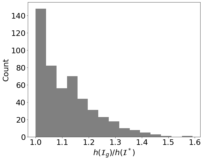
(a) a

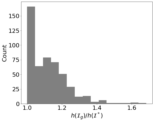
(b) b

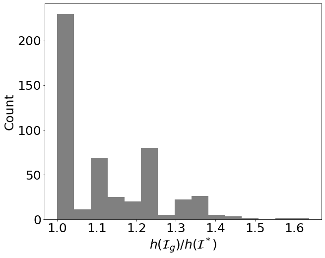
(c) c

Figure 1: Histograms of the ratio $h(\mathcal{I}_{g})/h(\mathcal{I}^{*})$.

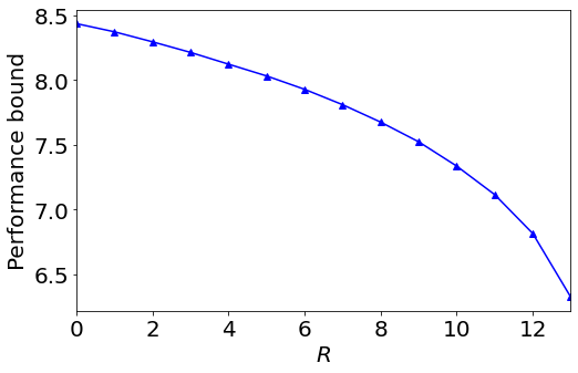
Figure 2: Performance bound for Algorithm 1 given by Theorem 8(d).

Similarly, we plot the results corresponding to Algorithm 2 when applied to the $500$ randomly generated BLDS instances as we described above. In addition, we set $\epsilon=0.1$ in Algorithm 2. Again, we observe from the histograms in Fig. 3 that Algorithm 2 works well on the randomly generated BLDS instances, and that as $R$ increases, Algorithm 2 yields better over all performance for the $500$ randomly generated BLDS instances. Here, we also note from the histogram in Fig. 3(b) that the ratio $h(\mathcal{I}_{f})/h(\mathcal{I}^{*})$ may be smaller than $1$ for certain BLDS instances (where recall that $h(\mathcal{I}_{f})$ is the cost of the solution $\mathcal{I}_{f}$ returned by Algorithm 2). This is because the solution $\mathcal{I}_{f}$ returned by Algorithm 2 only satisfies $z(\mathcal{I}_{f})\geq(1-\epsilon)z([n])$ (where $z([n])=z(\mathcal{I}^{*})$) as we argued in Theorem 2, which potentially implies that $z(\mathcal{I}_{f})<z(\mathcal{I}^{*})$ and $h(\mathcal{I}_{f})/h(\mathcal{I}^{*})<1$. Nonetheless, we observe from our experiments that for more than $99\%$ of the $1500$ random BLDS instances (with $R\in\{1,5,10\}$), the constraint $z(\mathcal{I}_{f})=z([n])$ is satisfied. Moreover, we have from the arguments in Section 3.3 that the performance bound for Algorithm 2 given by Theorem 9(b) can be written as $h(\mathcal{I}_{f})\leq\frac{1}{1-\epsilon}(1+\ln z^{\prime}([n]))h(\mathcal{I}_{*})$, where $z^{\prime}(\cdot)$ is defined in (31) and we set $\epsilon=0.1$. In Fig. 4, we plot the performance bound of Algorithm 2, i.e., $\frac{1}{1-\epsilon}(1+\ln z^{\prime}([n]))$, averaged over the $500$ random BLDS instances, for $R$ ranging from $0$ to $13$. We also see from Fig. 4 that the value of the performance bound of Algorithm 2 decreases, i.e., the performance bound becomes tighter, as $R$ increases from $0$ to $13$. Although the performance bound in Theorem 9 is still a worst-case guarantee, the behavior of the bound again aligns with the actual performance of Algorithm 2 presented in Fig. 3, i.e., a tighter performance bound implies a better overall performance of the algorithm on the $500$ random BLDS instances.

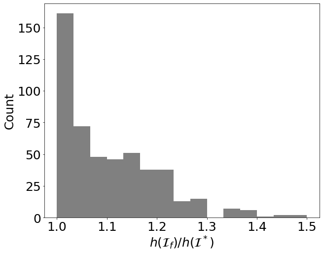
(a) a

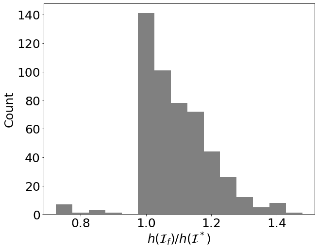
(b) b

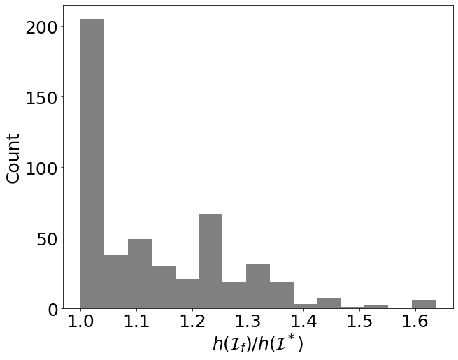
(c) c

Figure 3: Histograms of the ratio $h(\mathcal{I}_{f})/h(\mathcal{I}^{*})$.

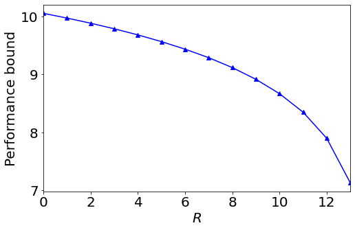
Figure 4: Performance bound for Algorithm 2 given by Theorem 9(b).

Putting the above results and discussions together, both of Algorithms 1 and 2 achieve good performance for the randomly generated BLDS instances, while Algorithm 2 achieves faster running times as we discussed in Section 3.2. Moreover, while the performance bound given in Theorem 8(d) for Algorithm 1 is tighter than that given in Theorem 9(b), both of the bounds provide insights into how the problem parameters of BLDS (e.g., the error bound $R$) influence the actual performance of the algorithms as we discussed above.

4 Conclusion

In this work, we considered the problem of data source selection for Bayesian learning. We first proved that the data source selection problem for Bayesian learning is NP-hard. Next, we showed that the data source selection problem can be transformed into an instance of the submodular set covering problem, and can then be solved using a standard greedy algorithm with provable performance guarantees. We also proposed a fast greedy algorithm that improves the running times of the standard greedy algorithm, while achieving comparable performance guarantees. The fast greedy algorithm can be applied to solve the general submodular set covering problem. We showed that the performance bounds provide insights into the actual performances of the algorithms under different instances of the data source selection problem. Finally, we validated our theoretical analysis using numerical examples, and showed that the greedy algorithms work well in practice.

5 Appendix

5.1 Extension to Non-Bayesian Learning

Let us consider a scenario where there is a set of agents, denoted as $[n]$, who wish to collaboratively learn the true state of the world. The agents interact over a directed graph $\mathcal{G}=([n],\mathcal{E})$, where each vertex in $[n]$ corresponds to an agent and a directed edge $(j,i)\in\mathcal{E}$ indicates that agent $i$ can (directly) receive information from agent $j$. Denote $\mathcal{N}_{i}\triangleq\{j:(j,i)\in\mathcal{E},j\neq i\}$ as the set of neighbors of agent $i$. Suppose each agent has an associated data source with the same observation model as described in Section 2. Specifically, the observation (conditioned on the state $\theta\in\Theta$) provided by the data source at agent $i$ at time step $k\in\mathbb{Z}_{\geq 1}$ is denoted as $\omega_{i,k}\in S_{i}$, which is generated by the likelihood function $\ell_{i}(\cdot|\theta)$. Each agent $i\in[n]$ is assumed to know $\ell_{i}(\cdot|\theta)$ for all $\theta\in\Theta$. Similarly, we consider the scenario where using the data source of agent $i\in[n]$ incurs a cost denoted as $h_{i}\in\mathbb{R}_{>0}$ for all $i\in[n]$, and there is a (central) designer who can select a subset $\mathcal{I}\subseteq[n]$ of agents whose data sources will be used to collect observations. We assume that the designer knows $\ell_{i}(\cdot|\theta)$ for all $i\in[n]$ and for all $\theta\in\Theta$. After set $\mathcal{I}\subseteq[n]$ is selected, each agent $i\in[n]$ updates its belief of the state of the world, denoted as $\mu^{\mathcal{I}}_{i,k}(\cdot)$, using the following distributed non-Bayesian learning rule as described in [20]:

$$\mu_{i,k+1}^{\mathcal{I}}(\theta)=\frac{\prod_{j=1}^{n}(\mu_{j,k}^{\mathcal{I}}(\theta))^{a_{ij}}\ell_{i}(\omega_{i,k+1}|\theta)}{\sum_{\theta_{p}\in\Theta}\prod_{j=1}^{n}(\mu_{j,k}^{\mathcal{I}}(\theta_{p}))^{a_{ij}}\ell_{i}(\omega_{i,k+1}|\theta_{p})}\ \forall\theta\in\Theta,$$ (35)

where $\mu_{i,k}^{\mathcal{I}}(\theta)$ is the belief of agent $i$ that $\theta$ is the true state at time step $k$ when the set of sources given by $\mathcal{I}\subseteq[n]$ is selected, and $a_{ij}$ is the weight that agent $i\in[n]$ assigns to an agent $j\in\mathcal{N}_{i}\cup\{i\}$. Specifically, for any two distinct agents $i,j\in[n]$, $a_{ij}>0$ if agent $i$ receives information from agent $j$ and $a_{ij}=0$ otherwise, where $\sum_{j\in\mathcal{N}_{i}\cup\{i\}}a_{ij}=1$. Note that if agent $i\notin\mathcal{I}$, i.e., the data source of agent $i$ is not selected to collect observations, we set $\ell_{i}(s_{i}|\theta_{p})=\ell_{i}(s_{i}|\theta_{q})$ for all $\theta_{p},\theta_{q}\in\Theta$ and for all $s_{i}\in S_{i}$. Similarly, for any $i\in[n]$, the initial belief is set to be $\mu_{i,0}^{\mathcal{I}}(\theta)=\mu_{i,0}(\theta)$ for all $\mathcal{I}\subseteq[n]$ and for all $\theta\in\Theta$, where $\sum_{\theta\in\Theta}\mu_{i,0}(\theta)=1$ and $\mu_{i,0}(\theta)\in\mathbb{R}_{\geq 0}$ for all $\theta\in\Theta$. We then see from (35) that $\sum_{\theta\in\Theta}\mu^{\mathcal{I}}_{i,k}(\theta)=1$ and $0\leq\mu_{i,k}^{\mathcal{I}}(\theta)\leq 1$ for all $k\in\mathbb{Z}_{\geq 0}$, for all $\theta\in\Theta$ and for all $\mathcal{I}\subseteq[n]$. Moreover, for a given true state $\theta\in\Theta$, we define $F_{\theta}(i)=\{\theta_{p}\in\Theta:\ \ell_{i}(s_{i}|\theta_{p})=\ell_{i}(s_{i}|\theta),\forall s_{i}\in S_{i}\}$ for all $i\in[n]$. Similarly to Section 2, we denote $F_{\theta}(\mathcal{I})=\bigcap_{n_{i}\in\mathcal{I}}F_{\theta}(n_{i})$, where we also assume that Assumption 1 holds for the analysis in this section. Again, note that $F_{\theta}(\emptyset)=\Theta$, and $\theta\in F_{\theta}(\mathcal{I})$ for all $\theta\in\Theta$ and for all $\mathcal{I}\subseteq[n]$. We have the following result.

Lemma 11.

Consider a set $[n]$ of agents interacting over a strongly connected graph $\mathcal{G}=([n],\mathcal{E})$. Suppose the true state of the world is $\theta^{*}$, $\mu_{i,0}(\theta)>0$ for all $i\in[n]$ and for all $\theta\in\Theta$, and $a_{ii}>0$ for all $i\in[n]$ in the rule given in (35). For any $\mathcal{I}\in[n]$, the rule given in (35) ensures that (a) $\mathop{\lim}_{k\to\infty}\mu^{\mathcal{I}}_{i,k}(\theta_{p})=0$ a.s. for all $\theta_{p}\notin F_{\theta^{*}}(\mathcal{I})$ and for all $i\in[n]$; and (b) $\lim_{k\to\infty}\mu^{\mathcal{I}}_{i,k}(\theta_{q})=\frac{\prod_{j=1}^{n}\mu_{j,0}(\theta_{q})^{\pi_{j}}}{\sum_{\theta\in F_{\theta^{*}}(\mathcal{I})}\prod_{j=1}^{n}\mu_{j,0}(\theta)^{\pi_{j}}}$ a.s. for all $i\in[n]$ and $\theta_{q}\in\ F_{\theta^{*}}(\mathcal{I})$, where $\pi\triangleq\begin{bmatrix}\pi_{1}&\cdots&\pi_{n}\end{bmatrix}^{\prime}$ satisfies $\pi^{\prime}A=\pi^{\prime}$ and $\|\pi\|_{1}=1$, and $A\in\mathbb{R}^{n\times n}$ is defined such that $A_{ij}=a_{ij}$ for all $i,j\in[n]$.

Proof.

We begin by defining the following quantities for all $\mathcal{I}\subseteq[n]$, for all $i\in[n]$ and for all $k\in\mathbb{Z}_{\geq 0}$:

$$\delta^{\mathcal{I}}_{i,k}(\theta)\triangleq\ln\frac{\mu^{\mathcal{I}}_{i,k}(\theta)}{\mu^{\mathcal{I}}_{i,k}(\theta^{*})}\ \text{and}\ \sigma_{i,k+1}(\theta)\triangleq\ln\frac{\ell_{i}(\omega_{i,k+1}|\theta)}{\ell_{i}(\omega_{i,k+1}|\theta^{*})},$$ (36)

where $\delta_{i,0}^{\mathcal{I}}(\theta)=\delta_{i,0}(\theta)\triangleq\ln\frac{\mu_{i,0}(\theta)}{\mu_{i,0}(\theta^{*})}$ for all $\mathcal{I}\subseteq[n]$. For any $\mathcal{I}\subseteq[n]$, we consider an agent $i\in[n]$ and $\theta_{p}\notin F_{\theta^{*}}(\mathcal{I})$. Following similar arguments to those for Theorem $1$ in [20], one can obtain that $\lim_{k\to\infty}\delta_{i,k}^{\mathcal{I}}(\theta_{p})=-\infty$ a.s., i.e., $\lim_{k\to\infty}\frac{\mu^{\mathcal{I}}_{i,k}(\theta_{p})}{\mu^{\mathcal{I}}_{i,k}(\theta^{*})}=0$ a.s. Since $0\leq\mu^{\mathcal{I}}_{i,k}(\theta)\leq 1$ for all $\theta\in\Theta$ and for all $k\in\mathbb{Z}_{\geq 0}$, it follows that $\lim_{k\to\infty}\frac{\mu^{\mathcal{I}}_{i,k}(\theta_{p})}{\mu^{\mathcal{I}}_{i,k}(\theta^{*})}\geq\lim_{k\to\infty}\mu^{\mathcal{I}}_{i,k}(\theta_{p})\geq 0$, which implies $0\leq\lim_{k\to\infty}\mu^{\mathcal{I}}_{i,k}(\theta_{p})\leq 0$ a.s., i.e., $\lim_{k\to\infty}\mu^{\mathcal{I}}_{i,k}(\theta_{p})=0$ a.s. This proves part (a).

We then prove part (b). For any $\mathcal{I}\subseteq[n]$, we now consider an agent $i\in[n]$ and $\theta_{q}\in F_{\theta^{*}}(\mathcal{I})$. Based on the definition of $F_{\theta^{*}}(\mathcal{I})$, we note that $\sigma_{i,k+1}(\theta_{q})=0,\forall k\in\mathbb{Z}_{\geq 0}$. We then obtain from (35) the following:

$$\delta^{\mathcal{I}}_{k+1}(\theta_{q})=A\delta^{\mathcal{I}}_{k}(\theta_{q}),$$

where $\delta^{\mathcal{I}}_{k}(\theta_{q})\triangleq\begin{bmatrix}\delta^{\mathcal{I}}_{1,k}(\theta_{q})&\cdots&\delta^{\mathcal{I}}_{n,k}(\theta_{q})\end{bmatrix}^{\prime}$. Moreover, we have

$$\lim_{k\to\infty}\delta^{\mathcal{I}}_{k}(\theta_{q})=(\lim_{k\to\infty}A^{k})\delta_{0}(\theta_{q})=\mathbf{1}_{n}\pi^{\prime}\delta_{0}(\theta_{q}),$$ (37)

where the last equality follows from the fact that $A$ is an irreducible and aperiodic stochastic matrix based on the hypotheses of the lemma. Simplifying (37), we obtain

$$\lim_{k\to\infty}\frac{\mu^{\mathcal{I}}_{i,k}(\theta_{q})}{\mu^{\mathcal{I}}_{i,k}(\theta^{*})}=\frac{\prod_{j=1}^{n}\mu_{j,0}(\theta_{q})^{\pi_{j}}}{\prod_{j=1}^{n}\mu_{j,0}(\theta^{*})^{\pi_{j}}}>0.$$ (38)

Summing up Eq. (38) for all $\theta_{q}\in F_{\theta^{*}}(\mathcal{I})$, we have

$$\lim_{k\to\infty}\frac{\sum_{\theta_{q}\in F_{\theta^{*}}(\mathcal{I})}\mu^{\mathcal{I}}_{i,k}(\theta_{q})}{\mu^{\mathcal{I}}_{i,k}(\theta^{*})}=\sum_{\theta_{q}\in F_{\theta^{*}}(\mathcal{I})}\frac{\prod_{j=1}^{n}\mu_{j,0}(\theta_{q})^{\pi_{j}}}{\prod_{j=1}^{n}\mu_{j,0}(\theta^{*})^{\pi_{j}}}>0.$$ (39)

Noting from part (a) that $\lim_{k\to\infty}\sum_{\theta_{q}\in\ F_{\theta^{*}}(\mathcal{I})}\mu^{\mathcal{I}}_{i,k}(\theta_{q})=1$ a.s., we see from (39) that $\lim_{k\to\infty}\mu^{\mathcal{I}}_{i,k}(\theta^{*})$ exists and is positive, a.s., which further implies via (38) that $\lim_{k\to\infty}\mu^{\mathcal{I}}_{i,k}(\theta_{q})$ exists and is positive, a.s. In other words, we have from (38) the following:

$$\frac{\mu^{\mathcal{I}}_{i,\infty}(\theta_{q})}{\mu^{\mathcal{I}}_{i,\infty}(\theta^{*})}=\frac{\prod_{j=1}^{n}\mu_{j,0}(\theta_{q})^{\pi_{j}}}{\prod_{j=1}^{n}\mu_{j,0}(\theta^{*})^{\pi_{j}}},$$ (40)

where $\mu^{\mathcal{I}}_{i,\infty}(\theta_{q})\triangleq\lim_{k\to\infty}\mu^{\mathcal{I}}_{i,k}(\theta_{q})$ for all $\theta_{q}\in F_{\theta^{*}}(\mathcal{I})$. Again noting that $\lim_{k\to\infty}\sum_{\theta\in\ F_{\theta^{*}}(\mathcal{I})}\mu^{\mathcal{I}}_{i,k}(\theta)=1$ a.s. for all $i\in[n]$, part (b) then follows from Eq. (40). ∎

Similarly to the problem formulation described in Section 2, we define the following error metric for the designer:

$$\bar{e}_{\theta^{*}}(\mathcal{I})=\sum_{i=1}^{n}e_{\theta^{*},i}(\mathcal{I}),$$

where $\theta^{*}$ is the true state, $e_{\theta^{*},i}(\mathcal{I})\triangleq\frac{1}{2}\mathop{\lim}_{k\to\infty}\|\mu^{\mathcal{I}}_{i,k}-\mathbf{1}_{\theta^{*}}\|_{1}$ and $\mu^{\mathcal{I}}_{i,k}\triangleq\begin{bmatrix}\mu^{\mathcal{I}}_{i,k}(\theta_{1})&\cdots&\mu^{\mathcal{I}}_{i,k}(\theta_{m})\end{bmatrix}^{\prime}$. In words, $\bar{e}_{\theta^{*}}(\mathcal{I})$ is the sum of the steady-state learning errors of all the agents in $[n]$, when the true state of the world is assumed to be $\theta^{*}$. It then follows from Lemma 11 that $\bar{e}_{\theta^{*}}(\mathcal{I})=n\big{(}1-\frac{\prod_{j=1}^{n}(\mu_{j,0}(\theta^{*}))^{\pi_{j}}}{\sum_{\theta\in F_{\theta^{*}}(\mathcal{I})}\prod_{j=1}^{n}(\mu_{j,0}(\theta))^{\pi_{j}}}\big{)}$ almost surely. Denoting

$$\bar{e}^{s}_{\theta_{p}}(\mathcal{I})\triangleq n\big{(}1-\frac{\prod_{j=1}^{n}(\mu_{j,0}(\theta_{p}))^{\pi_{j}}}{\sum_{\theta\in F_{\theta_{p}}(\mathcal{I})}\prod_{j=1}^{n}(\mu_{i,0}(\theta))^{\pi_{j}}}\big{)}\ \forall\theta_{p}\in\Theta,$$ (41)

we consider the following problem for the designer:

$$\begin{split}&\mathop{\min}_{\mathcal{I}\subseteq[n]}h_{\mathcal{I}}\\ &s.t.\ \bar{e}^{s}_{\theta_{p}}(\mathcal{I})\leq\bar{R}_{\theta_{p}},\forall\theta_{p}\in\Theta,\end{split}$$ (42)

where $0\leq\bar{R}_{\theta_{p}}\leq n$ and $\bar{R}_{\theta_{p}}\in\mathbb{R}$. Denoting $\bar{\mu}_{0}(\theta)\triangleq\prod_{i=1}^{n}\mu_{i,0}(\theta)^{\pi_{i}}$ for all $\theta\in\Theta$, we have from (41):

$$\bar{e}_{\theta_{p}}^{s}(\mathcal{I})=n(1-\frac{\bar{\mu}_{0}(\theta_{p})}{\sum_{\theta\in F_{\theta_{p}}(\mathcal{I})}\bar{\mu}_{0}(\theta)}),\forall\theta_{p}\in\Theta.$$ (43)

Now, we have from (7) and (43) that the optimization problem (42) can be viewed as an instance of Problem 1. Thus, all the theoretical results derived in this paper apply to this non-Bayesian distributed setting as well.

References

- Badanidiyuru and Vondrák [2014] A. Badanidiyuru and J. Vondrák. Fast algorithms for maximizing submodular functions. In Proc. ACM-SIAM Symposium on Discrete Algorithms, pages 1497–1514, 2014.
- Brémaud [2013] P. Brémaud. Markov chains: Gibbs fields, Monte Carlo simulation, and queues, volume 31. Springer Science & Business Media, 2013.
- Chaloner and Verdinelli [1995] K. Chaloner and I. Verdinelli. Bayesian experimental design: A review. Statistical Science, pages 273–304, 1995.
- Chepuri and Leus [2014] S. P. Chepuri and G. Leus. Sparsity-promoting sensor selection for non-linear measurement models. IEEE Transactions on Signal Processing, 63(3):684–698, 2014.
- Dasgupta [2005] S. Dasgupta. Analysis of a greedy active learning strategy. In Proc. Advances in Neural Information Processing Systems, pages 337–344, 2005.
- Feige [1998] U. Feige. A threshold of ln n for approximating set cover. Journal of the ACM (JACM), 45(4):634–652, 1998.
- Garey and Johnson [1979] M. R. Garey and D. S. Johnson. Computers and intractability: a guide to the theory of NP-Completeness. Freeman, 1979.
- Gelman et al. [2013] A. Gelman, J. B. Carlin, H. S. Stern, D. B. Dunson, A. Vehtari, and D. B. Rubin. Bayesian data analysis. Chapman and Hall/CRC, 2013.
- Golovin et al. [2010] D. Golovin, A. Krause, and D. Ray. Near-optimal Bayesian active learning with noisy observations. In Proc. Advances in Neural Information Processing Systems, pages 766–774, 2010.
- Jadbabaie et al. [2012] A. Jadbabaie, P. Molavi, A. Sandroni, and A. Tahbaz-Salehi. Non-Bayesian social learning. Games and Economic Behavior, 76(1):210–225, 2012.
- Jadbabaie et al. [2013] A. Jadbabaie, P. Molavi, and A. Tahbaz-Salehi. Information heterogeneity and the speed of learning in social networks. Columbia Business School Research Paper, (13-28), 2013.
- Khuller et al. [1999] S. Khuller, A. Moss, and J. S. Naor. The budgeted maximum coverage problem. Information Processing Letters, 70(1):39–45, 1999.
- Kononenko [1993] I. Kononenko. Inductive and Bayesian learning in medical diagnosis. Applied Artificial Intelligence an International Journal, 7(4):317–337, 1993.
- Krause and Cevher [2010] A. Krause and V. Cevher. Submodular dictionary selection for sparse representation. In Proc. International Conference on Machine Learning, pages 567–574, 2010.
- Krause et al. [2008] A. Krause, A. Singh, and C. Guestrin. Near-optimal sensor placements in Gaussian processes: Theory, efficient algorithms and empirical studies. Journal of Machine Learning Research, 9(Feb):235–284, 2008.
- Lalitha et al. [2014] A. Lalitha, A. Sarwate, and T. Javidi. Social learning and distributed hypothesis testing. In Proc. IEEE International Symposium on Information Theory, pages 551–555, 2014.
- Liu et al. [2014] Q. Liu, A. Fang, L. Wang, and X. Wang. Social learning with time-varying weights. Journal of Systems Science and Complexity, 27(3):581–593, 2014.
- Mitra et al. [2020] A. Mitra, J. A. Richards, and S. Sundaram. A new approach to distributed hypothesis testing and non-Bayesian learning: Improved learning rate and Byzantine-resilience. IEEE Transactions on Automatic Control, 2020.
- Mo et al. [2011] Y. Mo, R. Ambrosino, and B. Sinopoli. Sensor selection strategies for state estimation in energy constrained wireless sensor networks. Automatica, 47(7):1330–1338, 2011.
- Nedić et al. [2017] A. Nedić, A. Olshevsky, and C. A. Uribe. Fast convergence rates for distributed non-Bayesian learning. IEEE Transactions on Automatic Control, 62(11):5538–5553, 2017.
- Nemhauser et al. [1978] G. L. Nemhauser, L. A. Wolsey, and M. L. Fisher. An analysis of approximations for maximizing submodular set functions—i. Mathematical Programming, 14(1):265–294, 1978.
- Palmer et al. [2004] J. Palmer, B. D. Rao, and D. P. Wipf. Perspectives on sparse Bayesian learning. In Proc. Advances in Neural Information Processing Systems, pages 249–256, 2004.
- Wolsey [1982] L. A. Wolsey. An analysis of the greedy algorithm for the submodular set covering problem. Combinatorica, 2(4):385–393, 1982.
- Ye and Sundaram [2019] L. Ye and S. Sundaram. Sensor selection for hypothesis testing: Complexity and greedy algorithms. In Proc. IEEE Conference on Decision and Control, pages 7844–7849, 2019.
- Ye et al. [2020] L. Ye, N. Woodford, S. Roy, and S. Sundaram. On the complexity and approximability of optimal sensor selection and attack for Kalman filtering. IEEE Transactions on Automatic Control, 2020.