Cophasing multiple aperture telescopes with Linearized Analytic Phase Diversity (LAPD)

Abstract

Focal plane wavefront sensing is an appealing technique to cophase multiple aperture telescopes. Phase diversity, operable with any aperture configuration or source extension, generally suffers from high computing load. In this Letter, we introduce, characterize and experimentally validate the LAPD algorithm, based on a fast linearized phase diversity algorithm We demonstrate that a typical performance of $\lambda/75$ RMS wavefront error can be reached.

1 Introduction

Segmentation of the primary mirror is an inevitable step for space or ground-based optical telescopes in order to maximize the pupil diameter and therefore increase their spatial resolution and collecting power. This was implemented for the Keck telescopes [1] on the ground, or the soon-to-be-launched James Webb Space Telescope (JWST) [2], and it prevails in the design of the future extremely large optical telescope projects [3, 4]. For other projects [5], the goal is to minimize the volume at launch.

A critical sub-system of such instruments is the Cophasing Sensor (CS), whose goal is to measure low order aberrations (i.e. local piston tip and tilt) corresponding to relative positioning errors of the sub-apertures. We make the assumption that the optical quality of each sub-aperture is sufficient so that the high order aberrations are negligible; for example, high technology readiness level of requirements for the JWST segments is a mirror quality with less than 23.7nm RMS error [6]. Several steps are usually required to bring the instrument from a potentially very disturbed state (where images of each sub-aperture are scattered in the focal plane) to the optimal phased state with phasing errors within a small fraction of the operation wavelength (typically below $\lambda/40$ RMS according to a typical error budget for multi-aperture systems [7]). Therefore, different algorithms are being investigated to correct for aberrations during each step [8].

For the fine phasing step, Phase Diversity (PD) [9, 10] is a very appealing and much studied CS [11, 12, 13, 14, 15, 16, 17, 18] for several reasons: firstly, this CS can use the scientific camera; this both simplifies the hardware and avoids differential aberrations between the scientific sensor and the CS. Secondly, it is appropriate for an instrument with a large number of sub-apertures, because the complexity of the hardware does not scale with the number of sub-apertures and remains essentially independent of it, contrarily to the case of common pupil-plane sensors [13]. Finally, even if this letter only addresses the case of an unresolved object, it can be used on very extended objects, for which it is actually the only reasonable CS [17]. However, since the link between the aberrations and the focal and extrafocal images that are analyzed is highly non-linear, PD usually requires time-consuming, high computational cost, iterative minimization algorithms.

Before PD can be applied, the sub-apertures must be coarsely (geometrically) aligned. For this step, Vievard et al. [19] developed the ELASTIC algorithm. The latter allows to reduce large tip/tilt aberrations over sub-apertures from several $\lambda$ RMS to less than $\lambda/8$ RMS when observing an unresolved target. In this case, Mocœur et al. [20] proved through simulations that usual PD equations could be linearized, and the algorithm thus made much simpler, and incomparably quicker for whichever observed object (resolved or unknown and unresolved). Other methods, like Fast and Furious [15, 21], also exploited the small aberration regime to implement a fast estimator for wavefront sensing and control but it does not allow open loop estimation, and is limited to unresolved sources.

In this Letter we present a new algorithm similar to the Newton-Raphson method [22] and based on Mocœur et al. [20]. We derive and discuss the algorithm, numerically characterize it, and finally we present the first lab experimental validation of linearized PD on a multi-aperture telescope.

2 The linearized phase diversity principle

The idea behind the new algorithm is to iteratively apply the linearized PD [20] around the last estimated set of aberrations. Concretely, it means that a first set of aberrations would be estimated and then used as starting point to derive a new estimate. A few iteration of this method is expected to help increasing the capture range of the linearized PD.

Following Mocœur et al. [20] we begin by performing a $1^{rst}$ order Taylor expansion of the instrument Point Spread Function (PSF) $\boldsymbol{h}$, a vector defined on $N_{f}$ pixels, around the last known aberration state $\mathbf{a^{\prime}}$ as a function of the current aberration vector $\mathbf{a}$. With $\delta_{\textbf{a}}=\textbf{a}-\textbf{a'}$, we can write :

$$\boldsymbol{h}(\mathbf{a})=\boldsymbol{h}(\mathbf{a^{\prime}})+\operatorname{\mathbf{J}}_{\boldsymbol{h}}(\mathbf{a^{\prime}})\delta_{\textbf{a}}+o(\delta_{\textbf{a}})$$ (1)

where the vector of the Zernike coefficients of the residual perturbations we want to measure is $\mathbf{a}=(a_{0,0},a_{0,1},...,a_{k,n})$, with $k\in\left\{1,2,3\right\}$ the Zernike mode and $n$ the sub-aperture index. $\operatorname{\mathbf{J}}_{\boldsymbol{h}}(\mathbf{a^{\prime}})$ is the Jacobian matrix of $\boldsymbol{h}$ in $\mathbf{a^{\prime}}$: $\operatorname{\mathbf{J}}_{\boldsymbol{h}}=\left(\dfrac{\partial{\boldsymbol{h}}}{\partial{a_{0,0}}},\dfrac{\partial{\boldsymbol{h}}}{\partial{a_{0,1}}}...,\dfrac{\partial{\boldsymbol{h}}}{\partial{a_{k,n}}}\right)$.

Doing so, Mocœur showed that the best maximum likelihood estimator is the one that minimizes a criterion $L$, defined from the two diversity images $\boldsymbol{i}_{1}$ and $\boldsymbol{i}_{2}$, whose Fourier Transform (FT) are written as $\tilde{\boldsymbol{i}}_{1}$ and $\tilde{\boldsymbol{i}}_{2}$, as:

$$L(\mathbf{a}) =\dfrac{1}{2\sigma^{2}}\sum_{\nu}|\mathbf{A}(\nu)\mathbf{a}-\mathbf{B}(\nu)|^{2}+\mbox{Cst}$$ (2)

where $\sigma$ is the noise variance in each image, supposedly the same in both, $\nu$ is the spatial frequency index, and

$\mathbf{A}(\nu)=\dfrac{\tilde{\boldsymbol{i}}_{2}(\nu)\text{\boldmath$\alpha$\unboldmath}_{1}(\nu)-\tilde{\boldsymbol{i}}_{1}(\nu)\text{\boldmath$\alpha$\unboldmath}_{2}(\nu)}{\sqrt{|\text{\boldmath$\beta$\unboldmath}_{1}(\nu)|^{2}+|\text{\boldmath$\beta$\unboldmath}_{2}(\nu)|^{2}+\epsilon}}$ and $\mathbf{B}(\nu)=\dfrac{\tilde{\boldsymbol{i}}_{1}\text{\boldmath$\beta$\unboldmath}_{2}(\nu)-\tilde{\boldsymbol{i}}_{2}(\nu)\text{\boldmath$\beta$\unboldmath}_{1}(\nu)}{\sqrt{|\text{\boldmath$\beta$\unboldmath}_{1}(\nu)|^{2}+|\text{\boldmath$\beta$\unboldmath}_{2}(\nu)|^{2}+\epsilon}}$

with, for $i\in\{1,2\}$ (each diversity plane), $\text{\boldmath$\alpha$\unboldmath}_{i}=FT[\operatorname{\mathbf{J}}_{\boldsymbol{h}_{i}}]\mbox{ and }\text{\boldmath$\beta$\unboldmath}_{i}=FT[\boldsymbol{h}_{i}]$.

$\mathbf{A}(\nu)$ is a $(k_{max}\mathcal{N}_{a})$ vector (with $k_{max}$ the highest Zernike mode considered and $\mathcal{N}_{a}$ the number of sub-apertures) defined for each $\nu$ value. We can concatenate all $\mathbf{A}(\nu)$ vectors to obtain a $\mathbf{A}$ matrix with $(N_{f},k_{max}\mathcal{N}_{a})$ dimensions. $\mathbf{A}$ corresponds to the part of the criteria that explicitly depends on the sought aberrations. $\mathbf{B}(\nu)$ is a scalar and is used to compute the vector (with a length of $N_{f}$) $\mathbf{B}$ corresponding to the criteria expression when there are no aberrations. $\epsilon$ is set to $10^{-6}$, allowing the criteria not to diverge for high frequencies.

Since $L$ is quadratic, the derivation of its gradient with respect to the aberrations leads to a simple linear equation depending on $\mathbf{a}$. Therefore, the latter can be estimated analytically thanks to the least square solution for complex data:

$$\hat{\mathbf{a}}=\left[\Re(\mathbf{A}^{H}\mathbf{A})\right]^{\dagger}.\left[\Re(\mathbf{A}^{H}\mathbf{B})\right]$$ (3)

with $\Re$ the real part and $\dagger$ the matrix generalized inverse.

Here, we compute the latter with the Singular Value Decomposition. In this process, we can filter out singular modes whose singular values are too small and lead to noise amplification in the inversion. We show Fig. 1 the filtered modes for a 6 circular aperture instrument. We can see that the filtered modes, not seen by the system, are as expected the global piston, tip and tilt.

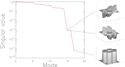
Figure 1: Singular values associated with each modes. The three lowest singular values showed for a 6 circular sub-aperture system correspond to global tip, global tilt and global piston.

We found that range and accuracy could be notably increased by performing a few internal iterations (typically from 1 to 3 as we will show in the following section): a first set of aberrations (noted $\mathbf{a^{\prime}}$) is estimated, and used as initial guess for a new estimation. It means that the Taylor expansion is then performed around $\mathbf{a^{\prime}}$ (Eq. (1)). We call this algorithm LAPD for Linearized Analytical Phase Diversity.

3 Numerical validation

The optimization and performance evaluations of LAPD are based on a compact pupil with 18 circular sub-apertures placed on a hexagonal grid (see Fig. 2 - left) and compared to a ”classic” iterative PD algorithm [10] for an observation of an unresolved source. All our tests are performed with a simulation tool that simulates the pupil, the phase map error in the pupil plane and that generates images of a point source using the Fraunhofer diffraction theory [23] . The size of the images is $64$ by $64$ pixels, with photon noise and a read-out-noise of $5$ photo-electrons. For an initial purpose of metrology tests we will consider high illumination of $5\times 10^{5}$ photo-electrons per image corresponding to a Signal-to-noise ratio of around 700. No higher order aberration are taken into account in our tests here.

3.1 Phase diversity optimization

We start with the optimization of the defocus introduced between the focal plane image and the diversity image. PD algorithms are based upon the difference between those two images. If this difference is not large enough, performance of such algorithms is poor. In order to find the optimal defocus for LAPD, we fix a random piston/tip/tilt aberration set with a 0.1 rad RMS standard deviation and study the estimation error for various defocus values. For each value of defocus we perform $\mathcal{N}_{o}=50$ noise and perturbation draws. Fig. 2 shows the evolution of LAPD and classic PD algorithm estimation root mean square error (RMSE) in regards of the defocus between images.

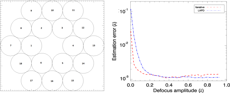
Figure 2: Left: Simulated 18 compact circular sub-apertures. Right : Defocus amplitude optimization for LAPD and the classic PD.

We can see that the tendency of both algorithms is that their estimation error decreases when the defocus increases, until a minimal plateau. The latter minimum is slightly above $\lambda/1000$ RMS for both algorithm when the defocus amplitude is larger than $0.2\lambda$. This result is in adequation with previous work [24] on optimal defocus diversity in the case of a monolithic telescope. In the following we will use a $0.3\lambda$ defocus amplitude.

3.2 Linearity of the sensor

Let us now study the linearity and dynamic range of LAPD. We study the LAPD estimation using $0$ to several internal iterations for a piston and a tilt error range of $\left[-0.5\lambda;0.5\lambda\right]$. Fig. 3 shows the evolution of the mean estimation over $\mathcal{N}_{o}=50$ noise draws as a function of the introduced piston or tilt. We keep an illumination of $5\times 10^{5}$ photo-electrons per image for this test.

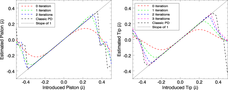
Figure 3: Evolution of the piston () and tilt () estimation as a function the introduced piston or tilt.

On Fig. 3 (left) we can see that LAPD without internal iteration has a linear response on the $\left[-0.2\lambda;0.1\lambda\right]$ piston range. Increasing the number of internal iterations enlarges LAPD linear range to about $\left[-0.4\lambda;0.35\lambda\right]$. More than 3 internal iterations do not increase the dynamic range. We also over-plot the linear range of the classic PD $\left[-0.45\lambda;0.4\lambda\right]$. The asymmetry that we notice in the linear range comes from the choice of the small unilateral defocus as a phase diversity. Indeed, further tests showed that the linear range will be symmetric only in the case of a symmetric diversity (two diversity images with opposite defocus) or by increasing the defocus to several $\lambda$s. On Fig. 3 (right) we see that LAPD tilt estimation is linear on the $\left[-0.1\lambda;0.1\lambda\right]$ range without internal iteration. When increasing the number of internal iterations to 3 the tilt estimation is linear on the $\left[-0.32\lambda;0.32\lambda\right]$ range, just like the classic PD. We then showed that LAPD piston or tilt estimation is linear on a given dynamic range and the latter can be increased by using more internal LAPD iterations. Doing so, LAPD dynamic range is comparable to classic phase diversity algorithm’s for tilt estimation. The dynamic range of the piston estimation does not reach the same as the classic PD, however we can assume that static phasing errors would not be as large during the telescope fine phasing step.

3.3 Noise propagation study

Finally, we study the performance of LAPD with regards to the photo-electron count ($\mathcal{N}_{ph}$). We set the number of internal iterations to two, as we saw previously that it is sufficient to significantly increase the capture range of the algorithm. For each case we study the standard deviation and the RMSE of the piston/tip/tilt estimation over the $\mathcal{N}_{o}=50$ draws. A random piston/tip/tilt set with a 0.2 rad standard deviation is applied for each estimation. Fig. 4 left and right respectively show the evolution of the standard deviation and the RMSE as a function of the number of photo-electrons in each image.

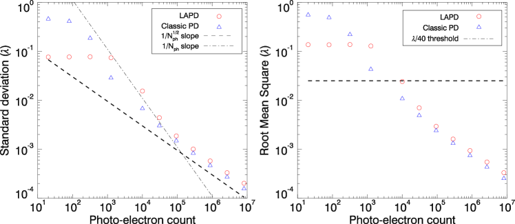
Figure 4: LAPD propagation study. Evolution of the standard deviation (left) and RMSE (right) of the estimation as a function of image illumination.

We can distinguish different regimes in the standard deviation evolution of the LAPD and classic PD estimations: at low flux (below $10^{3}$ photo-electrons for LAPD, below $5\times 10^{2}$ photo-electrons for the classic PD) the standard deviation of the estimation is constant. The value of the standard deviation is around $\lambda/16$ for LAPD and around $\lambda/5$ for the classic PD. This difference can be explained by the fact that the few number of iterations for LAPD can play the role of regulation [25]. Since the classic PD does not have any kind of regularisation, the performance at low flux is significantly worse. At high flux ($\mathcal{N}_{ph}>10^{4}$, respectively $\mathcal{N}_{ph}>10^{5}$), the slope of detector-noise (respectively shot-noise) regime is clearly evidenced in the case of LAPD estimation standard deviation. In the case of the classic PD, the shot-noise regime is evidenced for $\mathcal{N}_{ph}>10^{4}$. The evolution of the RMSE informs us that the estimation error is $<\lambda/40$ for an illumination $>~{}10^{3}$ photo-electrons for the classic PD and $>10^{4}$ photo-electrons in the case of LAPD. Both algorithms have similar behaviors. However we can notice that the classic PD algorithm is slighly more accurate when the flux is above $3\times 10^{5}$. This difference is reduced (even ) by using LAPD with more internal iterations.
In this section the LAPD implementation (2 internal iterations, unoptimized IDL code) runs about $3\times$ faster than the classic PD. The main bottleneck is the sequential computation of FTs for $\text{\boldmath$\alpha$\unboldmath}_{i}$. For the future, this should trivially be parallelizable for manycore architectures with little overhead.

4 Experimental validation

In order to experimentally validate LAPD, we use the BRISE bench built by Onera [26, 19]. We conduct tests imaging the collimated output of a fibered single-mode fiber near 635 nm, acting like an unresolved source, through six circular apertures of a segmented mirror. Each segment is supported by three piezoelectric actuators, allowing to introduce piston, tip or tilt perturbations. Downstream, a phase diversity module is used to simultaneously form a focused and a defocused image of the object on a $1300\times~{}1000$ pixels camera, from which we extract two $128\times~{}128$ diversity images. We test LAPD with a $0.3\lambda$ defocus between the two images, and no internal iteration.

A closed-loop sequence is performed to correct piston/tip/tilt perturbations since it is not possible to perform a single-step correction, due to not perfectly deterministic active mounts.

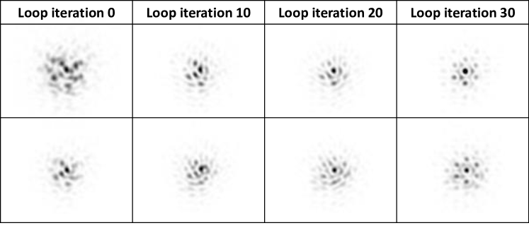
Figure 5: Experimental validation of LAPD: focal (top) and defocused (bottom) PSF evolution during iterations of a closed-loop correction on a 6-subaperture mirror bringing the global phase error down to a $\lambda/75$ RMS.

Figure 5 shows the effect of LAPD correction. The departure point (iteration 0) of the cophasing sequence results from the previous coarse alignment [19, 27], where we can see small piston/tip/tilt errors from the PSF shape. The loop is closed with a pure integrator with $0.2$ gain. We can see over the loop iterations that LAPD manages to estimate the small errors to reach the phased instrument PSF. The estimated piston/tip/tilt errors over the sub-aperture have a maximal amplitude of $0.1\lambda$ at the beginning of the loop closure, and are brought to less than $0.02\lambda$, with a $\lambda/75$ RMS dispersion. The total flux is $10^{6}$ photo-electrons. A comparison of the obtained dispersion ($\lambda/75$) with the simulation in Fig. 4-left ($10^{-3}\lambda$) shows a difference of a factor 10. This difference can have several origins mainly linked to the simplified case used for simulation: 1- the error induced by the piezoelectric actuators ; 2- high order aberrations in the optical setup ; 3- bench modelization errors. Even with the hypothetical presence of these errors, LAPD was still able to bring the instrument in a finely cophased state.

5 Conclusion

We presented here LAPD, an analytical fast solution to the fine phasing of multi-aperture systems from a pair of diversity images near the focal plane. We showed with simulations on a 18-subaperture imager observing (for simplicity) an unresolved source that LAPD could increase its capture range with a small amount of internal iterations (typically less than 3), and that it can estimate piston/tip/tilt aberrations with an error below $\lambda/40$ RMS for an illumination $>10^{4}$ for $64\times 64$ pixel images. Finally, we validated LAPD on a 6-subaperture mirror. We showed that after correction of large alignment errors with ELASTIC we were able to bring the piston/tip/tilt errors down to less than $0.02\lambda$ RMS using a close-loop enslavement using LAPD. This work could be useful as an easy-to-implement, computationally efficient solution for the fine phasing of any multi-aperture telescope, and could also be used in the case of unresolved objects.

References

- [1] K. Matthews, A. M. Ghez, A. J. Weinberger, et al., “The First Diffraction-Limited Images from the W. M. Keck Telescope,” PASP 108(725), 615 (1996).
- [2] J. P. Gardner, J. C. Mather, M. Clampin, et al., “The James Webb Space Telescope,” Space Science Reviews 123, 485–606 (2006).
- [3] G. H. Sanders, “The thirty meter telescope (tmt): An international observatory,” Journal of Astrophysics and Astronomy 34, 81–86 (2013).
- [4] R. Gilmozzi and J. Spyromilio, “The european extremely large telescope (e-elt),” The Messenger 127(11), 3 (2007).
- [5] V. Villalba, H. Kuiper, and E. Gill, “Review on thermal and mechanical challenges in the development of deployable space optics,” JATIS 6(1), 010902 (2020).
- [6] H. P. Stahl, “JWST mirror technology development results,” in Optical Manufacturing and Testing VII, 6671, 11 – 22, International Society for Optics and Photonics, SPIE (2007).
- [7] J. E. Harvey and C. Ftaclas, “Fundamental limitations on off-axis performance of phased telescope arrays,” Proc. SPIE 1236, 390–405 (1990).
- [8] L. D. Feinberg, B. H. Dean, D. L. Aronstein, et al., “Trl-6 for JWST wavefront sensing and control,” in UV/Optical/IR Space Telescopes: Innovative Technologies and Concepts III, 6687, 668708, International Society for Optics and Photonics (2007).
- [9] R. A. Gonsalves, “Phase retrieval and diversity in adaptive optics,” Optical Engineering 21(5), 829–832 (1982).
- [10] L. M. Mugnier, A. Blanc, and J. Idier, “Phase diversity: a technique for wave-front sensing and for diffraction-limited imaging,” in Advances in Imaging and Electron Physics, P. Hawkes, Ed., 141, ch. 1, 1–76, Elsevier (2006).
- [11] R. G. Paxman and J. R. Fienup, “Optical misalignment sensing and image reconstruction using phase diversity,” J. Opt. Soc. Am. A 5(6), 914–923 (1988).
- [12] D. Redding et al., “Wavefront sensing and control for a Next Generation Space Telescope,” in Space Telescopes and Instruments V, P. Y. Bely and J. B. Breckinridge, Eds., 3356 (2), 758–772 (1998).
- [13] F. Cassaing, F. Baron, E. Schmidt, et al., “DARWIN Fringe Sensor (DWARF): Concept study,” in Towards Other Earths, SP-539, 389–392, ESA (2003).
- [14] L. Mugnier, F. Cassaing, B. Sorrente, et al., “Multiple-aperture optical telescopes: some key issues for Earth observation from a GEO orbit,” in 5th International Conference On Space Optics, SP-554, 181–187, CNES/ESA, ESA, (Toulouse, France) (2004).
- [15] V. Korkiakoski, C. U. Keller, N. Doelman, et al., “Fast & furious focal-plane wavefront sensing,” Applied optics 53(20), 4565–4579 (2014).
- [16] S. Meimon, E. Delavaquerie, F. Cassaing, et al., “Phasing segmented telescopes with long-exposure phase diversity images,” in Ground-based and Airborne Telescopes II, 7012, 701214, International Society for Optics and Photonics (2008).
- [17] L. Mugnier, F. Cassaing, G. Rousset, et al., “Continuous high-resolution Earth observation with multiple aperture optical telescopes,” in Proc. of the OPTRO 2005 International Symposium, AAAF, (Paris, France) (2005).
- [18] S. Egron, C.-P. Lajoie, L. Leboulleux, et al., “James webb space telescope optical simulation testbed iii: first experimental results with linear-control alignment,” in Space Telescopes and Instrumentation 2016: Optical, Infrared, and Millimeter Wave, 9904, 99044A, International Society for Optics and Photonics (2016).
- [19] S. Vievard, F. Cassaing, and L. M. Mugnier, “Large amplitude tip/tilt estimation by geometric diversity for multiple-aperture telescopes,” J. Opt. Soc. Am. A 34, 1272–1284 (2017).
- [20] I. Mocœur, L. M. Mugnier, and F. Cassaing, “Analytical solution to the phase-diversity problem for real-time wavefront sensing,” Optics Letters 34, 3487–3489 (2009).
- [21] S. P. Bos, S. Vievard, M. J. Wilby, et al., “On-sky verification of fast and furious focal-plane wavefront sensing: Moving forward toward controlling the island effect at subaru/scexao,” arXiv preprint arXiv:2005.12097 (2020).
- [22] T. J. Ypma, “Historical development of the newton–raphson method,” SIAM review 37(4), 531–551 (1995).
- [23] M. Born and E. Wolf, Principles of optics, Elsevier (2013).
- [24] D. J. Lee, M. C. Roggemann, and B. M. Welsh, “Cramer–rao analysis of phase-diverse wave-front sensing,” J. Opt. Soc. Am. A 16(5), 1005–1015 (1999).
- [25] Y. Yao, L. Rosasco, and A. Caponnetto, “On early stopping in gradient descent learning,” Constructive Approximation 26(2), 289–315 (2007).
- [26] F. Cassaing, B. Sorrente, L. Mugnier, et al., “Brise: a multipurpose bench for cophasing sensors,” in Advances in stellar interferometry, 6268, 62683A, International Society for Optics and Photonics (2006).
- [27] S. Vievard, F. Cassaing, L. M. Mugnier, et al., “Real-time full alignment and phasing of multiple-aperture imagers using focal-plane sensors on unresolved objects,” in Space Telescopes and Instrumentation 2018: Optical, Infrared, and Millimeter Wave, 10698, 1834 – 1844, International Society for Optics and Photonics, SPIE (2018).