Chen, Nadarajah, Pakiman, Jasin

Self-adapting Robustness in Demand Learning

Self-adapting Robustness in Demand Learning

Boxiao Chen, Selvaprabu Nadarajah, Parshan Pakiman College of Business Administration, University of Illinois at Chicago, Chicago, IL 60607, {bbchen, selvan, ppakim2}@uic.edu Stefanus Jasin Stephen M. Ross School of Business, University of Michigan, Ann Arbor, MI 48109, sjasin@umich.edu

We study dynamic pricing over a finite number of periods in the presence of demand model ambiguity. Departing from the typical no-regret learning environment, where price changes are allowed at any time, pricing decisions are made at pre-specified points in time and each price can be applied to a large number of arrivals. In this environment, which arises in retailing, a pricing decision based on an incorrect demand model can significantly impact cumulative revenue. We develop an adaptively-robust-learning (ARL) pricing policy that learns the true model parameters from the data while actively managing demand model ambiguity. It optimizes an objective that is robust with respect to a self-adapting set of demand models, where a given model is included in this set only if the sales data revealed from prior pricing decisions makes it “probable”. As a result, it gracefully transitions from being robust when demand model ambiguity is high to minimizing regret when this ambiguity diminishes upon receiving more data. We characterize the stochastic behavior of ARL’s self-adapting ambiguity sets and derive a regret bound that highlights the link between the scale of revenue loss and the customer arrival pattern. We also show that ARL, by being conscious of both model ambiguity and revenue, bridges the gap between a distributionally robust policy and a follow-the-leader policy, which focus on model ambiguity and revenue, respectively. We numerically find that the ARL policy, or its extension thereof, exhibits superior performance compared to distributionally robust, follow-the-leader, and upper-confidence-bound policies in terms of expected revenue and/or value at risk.

dynamic pricing, demand learning, self-adapting algorithm, robust optimization, risk management, regret minimization History: November 2020 (initial version).

1 Introduction

We consider a classical revenue management problem, where a product is sold over a finite number of periods and the selling price is adjusted over time. Specifically, we assume that some parameters of the demand distribution are unknown and belong to a finite set. The seller thus needs to learn the true value of these parameters from sales data. The dynamic pricing problem with demand learning is widespread in practice and has been considered by a number of papers in the literature (e.g., Bitran and Caldentey 2003, Elmaghraby and Keskinocak 2003, Araman and Caldentey 2010, den Boer 2015, Chen and Chen 2015, Feng and Shanthikumar 2018). In many of the existing papers, it is typical to assume that the number of periods is very large, and the firm can adjust the price at every period. Such price adjustments can be naturally interpreted as pricing at the individual customer level when the number of periods is taken to be the number of customers.

In this paper, we consider situations where changing the price at any arbitrary time may not be possible. Instead price can only be adjusted at pre-specified points in time. This is the case, for example, in brick-and-mortar stores selling fast-fashion products, where selling seasons lasting only three months or less (not very large) are very common. The store usually keeps the prices fixed during the day and does not perform intra-day updates as this may upset customers. Since the same price applies to all customers arriving on a given day, a few suboptimal prices based on an incorrect demand model could lead to losing a substantial fraction of the optimal revenue if the number of arrivals are high on that day. This feature fundamentally differentiates our setting from the standard demand learning literature and heightens the risk of losing revenue due to demand model ambiguity. The pricing setting we study is also relevant to omni-channel retailers that strive to sync online prices with in-store prices in response to customer frustration with price differences across these channels (see, e.g., McKinsey 2016 and Windstream Enterprise 2020). Such channel consistency would lead to infrequent online price changes and provide customers with a seamless transition when engaging in cross-channel shopping.

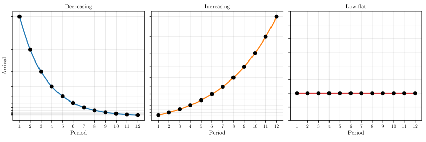
Figure 1: Illustration of customer arrival patterns.

Conceptually, the follow-the-leader learning (FTL; Shalev-Shwartz et al. 2011) and distributionally (static) robust optimization (SR; Scarf 1958, Goh and Sim 2010, Wiesemann et al. 2014) perspectives are relevant for pricing. The FTL approach chooses a price based on the best-estimate of the demand model parameters that are computed using sales data generated from prior pricing decisions. This strategy works well in periods where demand model ambiguity is low, but it can incur significant losses in periods when this ambiguity is high. On the other hand, a robust approach sets prices to maximize the worst-case revenue among a set of candidate demand models and thus mitigates risk when demand model ambiguity is high; however, it may lose significant revenue by being too conservative when such ambiguity is low. It is not possible to apriori determine when demand model ambiguity will be low. To illustrate, consider again, the fast-fashion example mentioned earlier. The arrival pattern of customers can take the decreasing, increasing, or low-flat patterns as shown in Figure 1, which correspond to the product being an early hit, a delayed hit, and a flop, respectively. Intuitively, the period by which the true demand model is identified with a sufficiently high probability via learning is earlier in the early-hit arrival pattern compared to the flop pattern. Once again, which arrival pattern will occur and when the true demand model will be identified is apriori unknown.

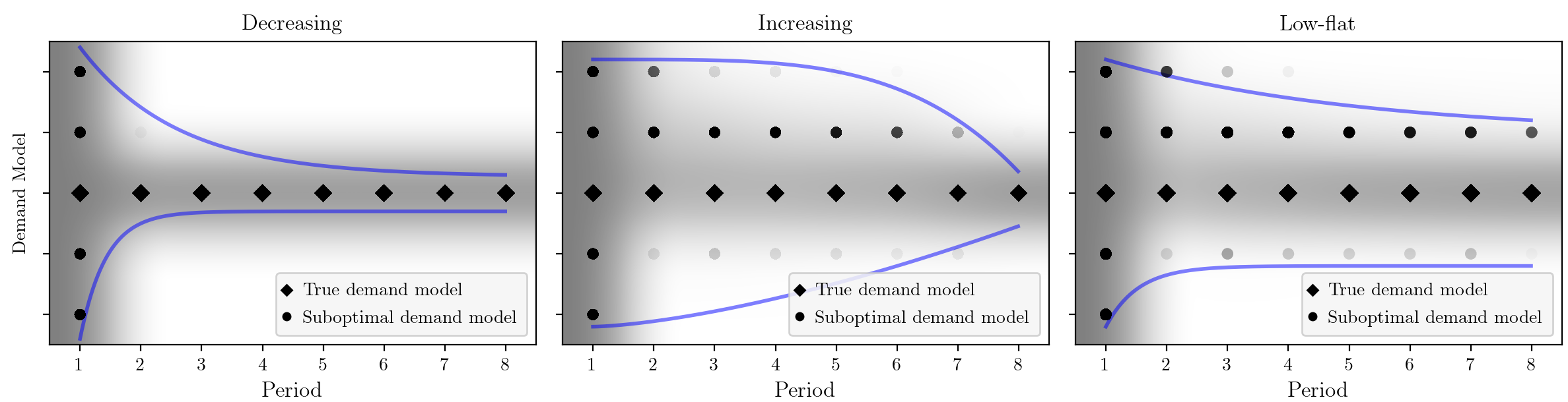
Figure 2: Evolution of ARL’s self-adapting ambiguity set over time for different arrival patterns. The darker regions indicate that a model is more probable to be in the ambiguity set.

To address this issue, we propose an adaptively-robust-learning (ARL) framework that (i) hedges the risk exposure to the seller when demand model ambiguity is high and (ii) gracefully transitions to regret minimization as this ambiguity diminishes upon receiving more data. Our approach does not require the knowledge of customer arrival patterns. The key idea in ARL is to use no-regret learning logic to maintain a “stochastic set” of demand models and choose prices that are robust with respect to the demand models in this set. Specifically, the set of demand models evolves in a stochastic manner based on the stream of sales data generated by past pricing decisions, with a given model being included in the set only if it is probable based on this data. This self-adapting set has the following appealing property: it consists of all candidate demand models and the true demand model when ambiguity is extremely high and essentially zero, respectively, and is a set in-between these two extremes as the demand model ambiguity decreases over time. Figure 2 illustrates how the aforementioned set of demand models evolves over time for the three arrival patterns shown in Figure 1. Since pricing decisions in our ARL framework are robust with respect to this stochastic set of demand models, it leverages the complementary strengths of no-regret learning and robust optimization, and as a consequence, has both favorable regret and risk properties.

1.1 Contributions

The contributions of this paper are highlighted below:

1. We propose a self-adapting framework for demand learning with limited price changes that actively manages revenue loss from model ambiguity. Our ARL framework assesses the revenue of a policy in period $t$ as the robust revenue with respect to a set of candidate demand models that evolves stochastically over time, adapting to the arrival of sales data and eliminating unlikely demand models from the set. We show that the definition of our self-adapting ambiguity set mitigates the potential error in the assessment of revenue resulting from this set not coinciding with the true demand model. In addition, we provide a probabilistic characterization of how this ambiguity set evolves over time as new data arrives: it starts from the set of candidate demand models and converges to a singleton set with the true demand model. Motivated by the aforementioned favorable properties, we define an ARL policy where the price in period $t$ is computed by optimizing the ARL revenue at this period. We derive a regret bound for the ARL policy, which highlights the impact of restricting price changes to pre-specified points in time. This is a unique feature in our dynamic pricing setting. At a high level, our ARL-regret upper bound depends on the arrival pattern of customers whereas the analogous regret upper bound would be independent of the arrival pattern if price changes are allowed at any time (see, e.g., Cheung et al. 2017).

2. We compare the objective optimized by the ARL policy against the objectives maximized by the SR and FTL policies, which focus on mitigating the risk of revenue loss and maximizing expected revenue, respectively. We begin by considering the case where the volume of customer arrivals is not at an extreme, that is, it is neither too large or too small. We establish that the ARL revenue is closer to the complete-information revenue (i.e., true but unknown revenue) than the SR revenue assessment in a probabilistic sense. This result shows that the ARL revenue is less conservative than the SR revenue. In addition, we show that the worst case deviation of the ARL revenue from the complete-information revenue is no worse than the analogous deviation of the FTL revenue. Therefore, using the ARL revenue as a proxy for the true revenue is less risky. We subsequently consider the case of extreme customer arrival volumes, establishing that (i) the ARL and SR objectives match each other when this volume is very low; and (ii) the ARL and FTL objectives match each other when this volume is very high. Collectively, our comparison of objectives shows that ARL bridges the gap between the SR and FTL pricing perspectives. By optimizing the ARL objective, the ARL policy is (i) risk-oriented when demand model ambiguity is high and the stochastic set of demand models is large and (ii) revenue-focused when demand model ambiguity is low and the stochastic set of demand models is small. We also discuss when we can expect the ARL policy performance to be superior to the SR and FTL policies in terms of expected revenue and the risk of revenue loss.

3. We numerically benchmark the ARL policy, and an extension thereof, with the SR, FTL, and upper-confidence-bound policies on a battery of instances that vary based on arrival patterns and demand model characteristics. The ARL-based policies improve on the FTL policy in terms of the expected complete-information revenue and the 5% value-at-risk of the revenue on most instances. They are competitive with the FTL policy on the remaining instances. Moreover, the ARL-based policies exhibit steeper improvements over the SR and upper-confidence-bound policies.

The trade-off between managing demand model ambiguity and expected revenue arises in contexts beyond dynamic pricing where parametric models of an uncertain quantity are needed. This includes demand response in electricity, valuation and portfolio optimization in finance, and other retail planning problems to name a few. Our ARL framework lays the ground work to manage this trade off and the key ideas are thus potentially relevant to these other application areas as well.

1.2 Novelty and Related Literature

Dynamic pricing with online demand learning has been studied extensively in the literature. Among several learning methods, first moment matching, which measures the distance between the empirical and model-based means, has been employed in Besbes and Zeevi (2009), Besbes and Zeevi (2012), Wang et al. (2014), Besbes and Zeevi (2015), Cheung et al. (2017), Chen et al. (2019a), Chen et al. (2019c), Lei et al. (2019), Chen et al. (2019b), and den Boer and Keskin (2019). It is also the estimation method utilized in this paper. FTL policies and its extensions constitute an important class of online learning algorithms (Blum 1998, Kalai and Vempala 2005), where first moment matching has been considered as a loss function (Besbes and Zeevi 2009, Besbes and Zeevi 2012, Cheung et al. 2017). The Upper Confidence Bound (UCB) algorithm, and variants thereof, have been widely implemented for bandit problems (Auer et al. 2002), as well as in the context of dynamic pricing (Zhang and Jasin 2018, Wang et al. 2020). We consider it as one of our benchmarks in the numerical study. A pervasive assumption made in the dynamic pricing with demand learning literature is that prices can be adjusted at any time, which justifies the focus on revenue maximization. In contrast, this research considers a novel dynamic pricing setting where price can only be adjusted at pre-specified points in time. Such pricing restrictions exist in practice. Managing both revenue and risk become important here and the proposed ARL framework addresses this need.

Our research adds to the distributionally robust optimization literature (Scarf 1958, Goh and Sim 2010, Wiesemann et al. 2014), where decisions are robust over an ambiguity set containing candidate models. More recent works in this literature have adopted several definitions of data-driven ambiguity sets (see, e.g., Pflug and Wozabal 2007, Delage and Ye 2010, Ben-Tal et al. 2013, Bertsimas et al. 2018, Esfahani and Kuhn 2018, Gupta 2019, Bu et al. 2020). These papers assume a batch data setting, that is, they assume a finite training set to construct the ambiguity set. The focus is on constructing such sets with finite-sample guarantees and computationally tractable optimization formulations. However, they do not consider the online arrival of new data and, therefore, there is no need to adaptively manage the trade-off between regret and risk over time. To the best of our knowledge, the combination of no-regret learning and robust optimization in our ARL framework to manage such a trade off adds a new online component to this literature.

Our paper also contributes to the growing interest in algorithms that embed solve intelligence. A key benefit of such intelligence is that it mitigates the need for hand-engineering (or tuning) algorithms to effectively solve different tasks and/or instances of a task. AlphaGo Zero by DeepMind for playing the game of Go is the most publicized recent success of solve intelligence. Here, the algorithm trains itself via self play instead of training on enormous amounts of game data, as done by past approaches (DeepMind 2017, Silver et al. 2017). AlphaGo Zero beats sophisticated Go agents and human masters of this game. Building algorithms with the notion of self adaptation to broaden their applicability and ease implementation is promising beyond Go and other games but such research has been limited (e.g., Chollet 2019; see also Pakiman et al. 2020 and Shah et al. 2020 for examples of self-adapting algorithms in the context of solving Markov decision processes and Markov games, respectively). Our research adds to this nascent literature by developing a self-adapting algorithm, ARL, to overcome implementation hurdles that arise in a dynamic pricing context due to limited price changes and demand model ambiguity. Without ARL’s mechanism to automatically manage the trade-off between regret and demand model risk, one could test if FTL and SR, or variations thereof, work on an instance-by-instance basis. However, this is not a generalizable implementation strategy, which we confirm in our numerical experiments.

2 Problem Formulation

Consider a firm selling a product over a finite horizon consisting of $T$ periods (e.g., weeks). At the beginning of every period $t\in\llbracket T\rrbracket\coloneqq\{1,2,\ldots,T\}$, the firm determines a price $p_{t}\in\mathcal{P}\coloneqq\{p^{1}\leq\cdots\leq p^{n}\}$ for the current period. The volume of customers in period $t$ is $N_{t}$. The $i$-th customer in period $t$ purchases a random quantity $D_{ti}(p_{t})$ at price $p_{t}$. The demand in period $t$ can then be written as the sum of these customer specific demands: $\sum_{i=1}^{N_{t}}D_{ti}(p_{t})$. The revenue during period $t$ is $R_{t}(p_{t})\coloneqq p_{t}\sum_{i=1}^{N_{t}}D_{ti}(p_{t})$. Given $(t,p_{t})\in\llbracket T\rrbracket\times\mathcal{P}$, $D_{ti}(p_{t})$ are independent and identically distributed for $i\in\llbracket N_{t}\rrbracket=\{1,2,\ldots,N_{t}\}$. We thus sometimes drop the index $i$ and use $D_{t}(p_{t})$ when referring to the distributional properties of these random variables. Let $\mathbb{E}_{D}[\cdot]$ denote expectation of the demand random variable within $[\cdot]$. We make the following common assumption regarding the true demand model.

For every $(t,p)\in\llbracket T\rrbracket\times\mathcal{P}$, random variable $D_{t}(p)$ is sub-exponential with parameters $(v,b)$, that is, for some $v,b\geq 0$ and every $\lambda\in(-{1}/{b},{1}/{b})$, we have:

$$\mathbb{E}_{D}\left[\exp(\lambda D_{t}(p))\right]\ \leq\ \exp\left({\lambda^{2}v^{2}}\big{/}{2}\right).$$

This assumption is mild and covers light-tailed demand distributions as well as most heavy-tailed distributions arising in applications (Foss et al. 2011, Chapter 3).

We describe the sequence of events for every time $t\in\llbracket T\rrbracket$ as follows:

1. At the beginning of period $t$, the firm makes pricing decision $p_{t}\in\mathcal{P}$;

2. Demand $D_{ti}(p_{t})$ realizes during period $t$ for each customer $i\in\llbracket N_{t}\rrbracket$;

3. After observing demands, the firm collects revenue $R_{t}(p_{t})$.

The firm’s objective is to maximize expected revenue over the planning horizon. Temporarily suppose we know the demand model $D_{t}$. Then, the task at hand is to find a policy $\pi$, which is a collection of prices decision rules $(p_{t}^{\pi}\in\mathcal{P},t\in\llbracket T\rrbracket)$, that solves

$$\max_{\pi}\ \sum_{t=1}^{T}\mathbb{E}_{p^{\pi}_{t},D}[R_{t}(p_{t}^{\pi})]\ =\ \max_{\pi}\ \sum_{t=1}^{T}\mathbb{E}_{p^{\pi}_{t},D}\left[p_{t}^{\pi}N_{t}D_{t}(p_{t}^{\pi})\right].$$ (1)

The expectation $\mathbb{E}_{p^{\pi}_{t},D}[\cdot]$ is taken with respect to both the price $p^{\pi}_{t}$ under policy $\pi$ and the demand random variable $D_{t}(p_{t}^{\pi})$.

In practice, there is demand model ambiguity. That is, the demand distribution $D_{t}(p_{t})$ is unknown and it is not possible to define (1) to compute an optimal dynamic pricing policy. We account for model ambiguity by assuming that the true demand model belongs to set $\{D_{t}(p;\theta):\theta\in\Theta\}$ parameterized by the vector $\theta$. This vector can take a finite number of values, represented by $\Theta\coloneqq\{\theta^{0},\theta^{1},\dots,\theta^{m}\}$. The revenue function corresponding to $\theta\in\Theta$ is $R_{t}(p_{t};\theta)\coloneqq p_{t}\sum_{i=1}^{N_{t}}D_{ti}(p_{t};\theta)$. The true demand model corresponds to $\theta^{0}$. In particular, we have $D_{t}(p)\equiv D_{t}(p;\theta^{0})$. The set of candidate demand models can either be constructed using practitioner knowledge or by leveraging the distributionally robust optimization literature.

Let $\mu_{t}(p;\theta):=\mathbb{E}_{D}[D_{t}(p;\theta)]$ and $r_{t}(p;\theta):=p\cdot\mu_{t}(p;\theta)$. In the rest of the paper, we impose the following technical assumption. For every $\theta\in\Theta\backslash\{\theta^{0}\}$, there exists a constant $c>0$ such that

$$\text{either}\hskip 28.45274pt\mu_{t}(p;\theta^{0})-\mu_{t}(p;\theta)\ \geq c,\hskip 38.41139pt\forall(t,p)\in\llbracket T\rrbracket\times\mathcal{P},$$

$$\text{or}\hskip 42.67912pt\ \mu_{t}(p;\theta^{0})-\mu_{t}(p;\theta)\ \leq-c,\hskip 28.45274pt\forall(t,p)\in\llbracket T\rrbracket\times\mathcal{P}.$$

Assumption 2 is a separability condition used to simplify analysis and guarantee that observing historical sales data allows first moment matching to differentiate the true demand model parameter $\theta^{0}$ from all the other parameters.

Remark 2.1

It is possible to weaken Assumption 2 by requiring:

$$\left|\mu_{t}(p;\theta^{0})-\mu_{t}(p;\theta)\right|\geq c,\hskip 28.45274pt\forall(t,p)\in\llbracket T\rrbracket\times\mathcal{P}.$$

All the theoretical results and policies in the paper will carry over with some minor changes and more involved theoretical statements and proofs.

Compared to the dynamic pricing literature, which allows price changes at any time, price modifications in the setting described above are only allowed at pre-specified points in time, for instance, each week over a selling season of three months. This aspect makes the customer arrival pattern important. We represent the arrival pattern over the selling season by a sequence $(N_{1},N_{2},\ldots,N_{T})$. The resulting total traffic is $M\coloneqq\sum_{t=1}^{T}N_{t}$. Consider a scenario where all arrivals occur in period $t=1$, that is, $M=N_{1}$. Since the true demand model is unknown in period one, the total revenue loss can be viewed as a loss per customer multiplied by the number of customers $M$, that is, this loss scales linearly with $M$. In general, revenue losses depend on the customer arrival pattern, which is apriori unknown. If price changes were instead possible at any time, then the price can be modified after every customer arrival and the revenue loss will thus be a constant and independent of $M$ (Proposition 1 in Cheung et al. 2017).

3 Adaptively Robust Learning Framework

In this section, we present an adaptively robust learning (ARL) framework to actively manage demand model ambiguity, which can vary over time in a manner that is a-priori unknown. For example, demand may be low in the initial days of the selling horizon, leading to a high demand model ambiguity, which subsequently declines quickly upon the arrival of a large number of customers. In §3.1, we define self-adapting ambiguity sets, which are the core objects used in the ARL framework. In §3.2, we investigate the stochastic evolution of these sets. In §3.3, we propose an ARL policy based on self-adapting ambiguity sets and establish a regret bound.

3.1 Self-adapting Ambiguity Sets and Revenue Assessment

Fix a policy $\pi$ and let $d^{\pi}_{ti}$ denote a realization of $D_{ti}(p^{\pi}_{t};\theta^{0})$. The empirical average demand at the beginning of period $t$ is $\big{(}\sum_{j=1}^{t-1}\sum_{i=1}^{N_{j}}d^{\pi}_{ji}\big{)}/\sum_{j=1}^{t-1}N_{j}$. Since data arrives sequentially, we compute the distance between the empirical average and the model-based mean for a given $\theta\in\Theta$ incrementally as follows. Let $\chi^{\pi}_{1}(\theta)\coloneqq 0$. For $t=2,\ldots,T$, we define $\chi^{\pi}_{t}(\theta)$ via the following recursion:

$$\chi^{\pi}_{t}(\theta)\coloneqq\chi^{\pi}_{t-1}(\theta)\ +\ \mu_{t-1}\left(p^{\pi}_{t-1};\theta\right)N_{t-1}\ -\ \sum_{i=1}^{N_{t-1}}d^{\pi}_{(t-1)i}.$$

Therefore, the distance between the empirical average and the mean demand is

$$\xi^{\pi}_{t}(\theta)\coloneqq\frac{|\chi^{\pi}_{t}(\theta)|}{\sum_{j=1}^{t-1}N_{j}}.$$ (2)

We construct an ambiguity set using the distance $\xi^{\pi}_{t}(\theta)$ and the following threshold that is a function of past arrivals:

$$\Phi\left(\sum_{j=1}^{t-1}N_{j}\right)\coloneqq\max\left\{\frac{\sqrt{2v^{2}\log\big{(}2MT\Psi(c)\big{)}}}{\sqrt{\sum_{i=1}^{t-1}N_{i}}},\frac{2b\log(2MT\Psi(c))}{\sum_{i=1}^{t-1}N_{i}}\right\},\qquad{\forall t=2,\dots,T,}$$

where

$$\Psi(c)\coloneqq\min\left\{{c^{2}}/{8v^{2}},{c}/{4b}\right\}$$

is a constant that depends on the separability constant $c$ (see Assumption 2) and the parameters $(v,b)$ of the true demand function (see Assumption 2). These constants can be estimated from the set $\Theta$. We write $\Phi$ and $\Psi$ to be functions of $\sum_{j=1}^{t-1}N_{j}$ and $c$, respectively, suppressing their dependence on other parameters for ease of notation. Let $\mathcal{U}_{t}^{\raisebox{1.0pt}{\scaleto{\pi}{2.8pt}}}\subseteq\Theta$ denote the ambiguity set at time $t\in\llbracket T\rrbracket$. We define $\mathcal{U}_{1}^{\raisebox{1.0pt}{\scaleto{\pi}{2.8pt}}}\coloneqq\Theta$ at the first stage and

$$\mathcal{U}_{t}^{\raisebox{1.0pt}{\scaleto{\pi}{2.8pt}}}\coloneqq\bigg{\{}\theta\in\Theta\ :\ \xi^{\pi}_{t}(\theta)\leq\Phi\bigg{(}\sum_{j=1}^{t-1}N_{j}\bigg{)}\bigg{\}}\cup\{\theta^{\pi}_{t}\},\qquad\forall t=2,\dots,T,$$ (3)

which includes the best estimator $\theta^{\pi}_{t}\coloneqq\arg\min_{\theta\in\Theta}\xi^{\pi}_{t}(\theta)$. If the distance ${\xi^{\pi}_{t}(\theta)}$ is smaller than the threshold $\Phi\big{(}\sum_{j=1}^{t-1}N_{j}\big{)}$, we view $\theta$ as being “probable” and include $\theta$ in $\mathcal{U}_{t}^{\raisebox{1.0pt}{\scaleto{\pi}{2.8pt}}}$. It is also possible that none of the candidate parameters satisfy this inequality, in which case we have $\mathcal{U}_{t}^{\raisebox{1.0pt}{\scaleto{\pi}{2.8pt}}}=\{\theta^{\pi}_{t}\}$. The specific value of the threshold $\Phi\big{(}\sum_{j=1}^{t-1}N_{j}\big{)}$ is chosen so that the excluded demand models are not probable given the currently available data (we will make the notion of probable precise in §3.2). It is easy to verify that $\Phi\big{(}\sum_{j=1}^{t-1}N_{j}\big{)}$ decreases in the data volume $\sum_{j=1}^{t-1}N_{j}$. Therefore, $\mathcal{U}_{t}^{\raisebox{1.0pt}{\scaleto{\pi}{2.8pt}}}$ is not very different from $\Theta$ when the data size is small (i.e., high demand model ambiguity) but becomes much smaller in size as the volume of data grows and demand model ambiguity decreases. Nevertheless, the demand models in set $\mathcal{U}_{t}^{\raisebox{1.0pt}{\scaleto{\pi}{2.8pt}}}$ change in a stochastic manner over time because the distance $\xi^{\pi}_{t}(\theta)$ depends on the demand realizations.

Fix a pricing policy $\pi$. Given a sequence of demand and price realizations $(p^{\pi}_{1},d^{\pi}_{1},\ldots,p^{\pi}_{T},d^{\pi}_{T})$ the self-adapting ambiguity sets can be used to evaluate the revenue along this trajectory as follows:

$$\sum_{t=1}^{T}\min_{\theta\in\mathcal{U}_{t}^{\raisebox{1.0pt}{\scaleto{\pi}{2.8pt}}}}r_{t}(p^{\pi}_{t};\theta)\ =\ \sum_{t=1}^{T}p^{\pi}_{t}N_{t}\min_{\theta\in\mathcal{U}_{t}^{\raisebox{1.0pt}{\scaleto{\pi}{2.8pt}}}}\mu_{t}(p^{\pi}_{t};\theta).$$

This revenue assessment accounts for the updates of the set $\mathcal{U}_{t}^{\raisebox{1.0pt}{\scaleto{\pi}{2.8pt}}}$ along the specified trajectory. In other words, this assessment adapts to the arrivals of data.

3.2 Interpretation and Evolution of Self-adapting Ambiguity Sets

We begin by analyzing the ambiguity set $\mathcal{U}_{t}^{\raisebox{1.0pt}{\scaleto{\pi}{2.8pt}}}$, which provides insight into the threshold used in its definition. We subsequently provide a probabilistic characterization of how this set evolves over time. Our analysis relies on the following definition.

Definition 3.1

The demand identification period is

$$\tilde{t}\coloneqq\min\left\{\min\left\{t\in\{2,\ldots,T\}:\ \sum_{j=1}^{t-1}N_{j}\geq\frac{\log\big{(}2MT\Psi(c)\big{)}}{\Psi(c)}\right\},\ T+1\right\}.$$

The period $\tilde{t}$ is the earliest time at which the volume of historical data exceeds ${\log(2MT\Psi(c))}/{\Psi(c)}$. If the inner optimization in the definition of $\tilde{t}$ is infeasible, then we have $\tilde{t}=T+1$. A key property of $\tilde{t}$ is that $\mathcal{U}_{\tilde{t}}^{\raisebox{1.0pt}{\scaleto{\pi}{2.8pt}}}=\{\theta^{0}\}$ holds with a probability level that mitigates the error in revenue assessment due to demand misidentification (i.e., $\mathcal{U}_{\tilde{t}}^{\raisebox{1.0pt}{\scaleto{\pi}{2.8pt}}}\neq\{\theta^{0}\}$). We elaborate on this property in Theorem 3.2 and the discussion that follows it.

Theorem 3.2

For any policy $\pi$ and $t\geq\tilde{t}$, $\mathcal{U}_{t}^{\raisebox{1.0pt}{\scaleto{\pi}{2.8pt}}}=\{\theta^{0}\}$ with a probability of at least $1-1/(MT\Psi(c))$.

The probability level $1-1/(MT\Psi(c))$ in Theorem 3.2 depends on the availability of data and the structure of demand curves through the terms $MT$ and $\Psi(c)$, respectively. This probability is large when the demand curves are well separated (i.e., $\Psi(c)$ is large) and/or the product of the number of periods $T$ and the store traffic $M$ is large. This probability can be small when the demand curves are very “close” to each other and the data volume is small, in which case the demand model cannot be learned even with low confidence. To exclude such cases, we make Assumption 3.2 in the rest of the paper. Parameters $M,T,$ $c$, $v$, and $b$ fulfill $\Psi(c)\geq\exp(1)/(2MT)$. Under this assumption, the probability $1-1/(MT\Psi(c))$ is at least $1-2/\exp(1)\approx 0.26$.

We now explain how the thresholds used in the definition of (3) and the choice of probability in Theorem 3.2 control the error in revenue assessment due to misidentifying the true demand model $\theta^{0}$. Fix a pricing policy $\pi$. Our revenue assessment error is given by

$$\mathrm{Error}^{\pi}\coloneqq\left|\sum_{t=1}^{T}\mathbb{E}_{p^{\pi}_{t}}[r_{t}(p^{\pi}_{t};\theta^{0})]\ -\ \sum_{t=1}^{T}\mathbb{E}_{p^{\pi}_{t},\mathcal{U}_{t}^{\raisebox{1.0pt}{\scaleto{\pi}{2.8pt}}}}\left[\min_{\theta\in\mathcal{U}_{t}^{\raisebox{1.0pt}{\scaleto{\pi}{2.8pt}}}}\ r_{t}(p^{\pi}_{t};\theta)\right]\right|,$$

where the first and second terms are the expected revenues under complete information (i.e., $\theta^{0}$ is known) and the ARL ambiguity set, respectively. Let

$$K_{0}\coloneqq\max_{(t,p,\theta)\in\llbracket T-1\rrbracket\times\mathcal{P}\times\Theta}\ \left|r_{t}(p;\theta^{0})\ -\ r_{t}(p;\theta)\right|$$

be the maximum revenue difference due to demand misidentification across all prices, periods, and demand models. Then, for any policy $\pi$, we have:

$$\mathrm{Error}^{\pi}\ \leq\ \;K_{0}\left[\mathbb{P}\Big{(}\exists t\in\llbracket\tilde{t}-1\rrbracket:\mathcal{U}_{t}^{\raisebox{1.0pt}{\scaleto{\pi}{2.8pt}}}\neq\{\theta^{0}\}\Big{)}\sum_{j=1}^{\tilde{t}-1}N_{j}\;+\right.$$

$$\left.\hskip 21.68121pt\mathbb{P}\Big{(}\exists t\in\llbracket T\rrbracket\setminus\llbracket\tilde{t}-1\rrbracket:\mathcal{U}_{t}^{\raisebox{1.0pt}{\scaleto{\pi}{2.8pt}}}\neq\{\theta^{0}\}\Big{)}\Big{[}M-\sum_{j=1}^{\tilde{t}-1}N_{j}\Big{]}\right],$$ (4)

where $\mathbb{P}(\cdot)$ is the probability operator. The right hand side of the inequality in (3.2) has two terms that bound the error due to misidentifying the demand model in periods before and after $\tilde{t}$, which are $\llbracket\tilde{t}-1\rrbracket$ and $\llbracket T\rrbracket\setminus\llbracket\tilde{t}-1\rrbracket=\{\tilde{t},\ldots,T\}$, respectively, as shown in Figure 4(b) (a). These terms are the product of the probability of misidentifying the demand model multiplied by the volume of arrivals in their respective time horizons. The misidentification probability $\mathbb{P}\big{(}\exists t\in\llbracket\tilde{t}-1\rrbracket:\mathcal{U}_{t}^{\raisebox{1.0pt}{\scaleto{\pi}{2.8pt}}}\neq\{\theta^{0}\}\big{)}$ before demand identification should be larger than the analogous probability $\mathbb{P}\big{(}\exists t\in\{\tilde{t},\ldots,T\}:\mathcal{U}_{t}^{\raisebox{1.0pt}{\scaleto{\pi}{2.8pt}}}\neq\{\theta^{0}\}\big{)}$ after such identification happens. Therefore, we bound the former quantity by $1$ and use concentration inequalities to upper bound the latter quantity by $2T\exp\big{(}-\sum_{t=1}^{\tilde{t}-1}N_{t}\Psi(c)\big{)}$, which is an exponentially decreasing function of the arrival volume (see the proof of Theorem 3.2 for details). These probability upper bounds are depicted in Figure 4(b) (a). We also bound $M-\sum_{j=1}^{\tilde{t}-1}N_{j}$ by the total volume $M$ as this replacement simplifies analysis and does not change the rate of our bound with respect to the scale of data, $M$. After these changes, we get

$$\mathrm{Error}^{\pi}\leq K_{0}\left[\sum_{t=1}^{\tilde{t}-1}N_{t}+2MT\exp\left({-\sum_{t=1}^{\tilde{t}-1}N_{t}\Psi(c)}\right)\right],$$

where the right hand side is a convex function of $\sum_{t=1}^{\tilde{t}-1}N_{t}$. To control the error due to demand model misidentification in the two horizons demarcated by $\tilde{t}$, we minimize this bound. The minimizer is $\sum_{t=1}^{\tilde{t}-1}N_{t}={\log(2MT\Psi(c))}/{\Psi(c)}$ and equals to the lower bound on the data volume used to define $\tilde{t}$ in Definition 3.1. Moreover, at this minimizer, (i) the bound of $2T\exp({-\sum_{t=1}^{\tilde{t}-1}N_{t}\Psi(c)})$ on the misidentification probability at a given period $t\in\{\tilde{t},\ldots,T\}$ equals $1/(MT\Psi(c))$, and (ii) the per-period probability of misidentification becomes $1/(MT\Psi(c))$, thus leading to the probability guarantee in Theorem 3.2. Finally, $\mathcal{U}_{t}^{\raisebox{1.0pt}{\scaleto{\pi}{2.8pt}}}$ equals the singleton $\{\theta^{0}\}$ with the latter probability because the threshold $\Phi\big{(}\sum_{i=1}^{t-1}N_{i}\big{)}$ is chosen to ensure that each incorrect demand model $\theta\neq\theta^{0}$ satisfies $\xi^{\pi}_{t}(\theta)>\Phi\big{(}\sum_{i=1}^{t-1}N_{i}\big{)}$ with a probability of at least $1-1/(MT\Psi(c))$ when $\sum_{j=1}^{t-1}N_{j}\geq{\log(2MT\Psi(c))}/{\Psi(c)}$. We refer interested readers to the proof of Theorem 3.2 for further details.

Figure 3: Illustration of the ambiguity set evolution.

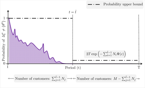
(a) Misidentification probability

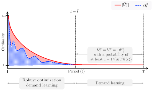
(b) Sizes of ambiguity set and bounding set

We now analyze the evolution of $\mathcal{U}_{t}^{\raisebox{1.0pt}{\scaleto{\pi}{2.8pt}}}$ as this set approaches the demand identification time. Recall that the elements in this set change stochastically as data arrives and so does its size. For $i\in\llbracket m\rrbracket$, define the distance of each candidate demand model $\theta^{i}$ from the true demand model $\theta^{0}$ as follows:

$$c^{i}\coloneqq\min_{{(t,p)\in\llbracket T-1\rrbracket\times\mathcal{P}}}\ \left|r_{t}(p;\theta^{0})\ -\ r_{t}(p;\theta^{i})\right|.$$ (5)

Then, $c^{i}>0$ due to Assumption 2. We use $c^{(1)}\leq\dots\leq c^{(m)}$ to represent an ascending ordering of these distances and use $\theta^{(i)}$ to denote the parameter that corresponds to $c^{(i)}$. Theorem 3.3 provides insight into the evolution of $\mathcal{U}_{t}^{\pi}$ using larger sets $\bar{\mathcal{U}}^{\pi}_{t}$. Let $\bar{\mathcal{U}}^{\pi}_{1}\coloneqq\mathcal{U}_{1}^{\pi}=\Theta$ for $t=1$, and define

$$\bar{\mathcal{U}}^{\pi}_{t}\coloneqq\begin{cases}\left\{\theta^{0},\theta^{(1)},\ldots,\theta^{(i^{*}-1)}\right\}&\quad\text{if }i^{*}\coloneqq\min\Big{\{}i\in\llbracket m\rrbracket:\sum\limits_{j=1}^{t-1}N_{j}\geq\frac{\log(2MT\Psi(c))}{\Psi(c^{(i)})}\Big{\}}\text{ is well-defined},\\[-14.0pt] \bar{\mathcal{U}}^{\pi}_{t-1}&\quad\text{otherwise,}\end{cases}$$

for each $t=2,3,\dots,T$. At period $t$, index $i^{*}$ identifies the closest demand model to $\theta^{0}$ (in terms of (5)) that can be eliminated with the same probability as Theorem 3.2 given the realized data. Theorem 3.3 connects ambiguity sets $\mathcal{U}_{t}^{\pi}$ to the bounding sets $\bar{\mathcal{U}}^{\pi}_{t}$, which are nested with a certain probability because the size $|\bar{\mathcal{U}}^{\pi}_{t}|$ of these sets are non-increasing with time. In contrast, the ambiguity sets $\mathcal{U}_{t}^{\pi}$ themselves cannot be guaranteed to be nested in general with this probability.

Theorem 3.3

For $t\geq 1$, we have $\mathcal{U}_{t}^{\pi}\subseteq\bar{\mathcal{U}}^{\pi}_{t}$ with a probability of at least $1-1/(MT\Psi(c))$.

The above theorem is a generalization of Theorem 3.2 as illustrated in Figure 4(b) (b). Specifically, it establishes the volume of arrivals $\sum_{j=1}^{t-1}N_{j}$ that is needed to ensure that a demand model (with a distance $c^{(i)}$) is eliminated from $\bar{\mathcal{U}}^{\pi}_{t}$, and hence $\mathcal{U}_{t}^{\pi}$, with a probability of at least $1-1/(MT\Psi(c))$. In contrast, Theorem 3.2 focuses on the data volume (see Definition 3.1) that is needed to eliminate all incorrect demand models with this probability. Therefore, despite the fact that the models included in the set $\mathcal{U}_{t}^{\pi}$ change in a stochastic manner, we can use the sets $\bar{\mathcal{U}}^{\pi}_{t}$ to “bound” this variation. In other words, it is likely that incorrect demand models will get progressively eliminated as more data is received. Moreover, consistent with intuition, demand models that are further away from the true demand model are likely to be removed before those that are closer to the true model.

3.3 Adaptively Robust Learning Policy

We now discuss an ARL policy that uses our self-adapting ambiguity sets in a manner that is consistent with a property of the optimal policy $\pi^{\text{CI}}$ in the complete information setting where $\theta^{0}$ is known. This property is that the price $p_{t}^{\text{CI}}$ prescribed by $\pi^{\text{CI}}$ at time $t\in\llbracket T\rrbracket$ solves the single-stage optimization problem

$$p_{t}^{\text{CI}}\coloneqq\argmax_{p\in\mathcal{P}}\ r_{t}(p;\theta^{0}).$$ (6)

In other words, the policy $\pi^{\mathrm{CI}}$ uses a fixed price $p_{t}^{\text{CI}}$ at period $t$. It is not difficult to see that the above price is optimal for (1). However, $\pi^{\text{CI}}$ is not computable since the objective function in (6) assumes the knowledge of $\theta^{0}$.

We define an ARL policy $\pi^{\text{ARL}}$ as follows. At time $t$, we set the price $p_{t}^{\mathrm{ARL}}$ to be

$$p_{t}^{\mathrm{ARL}}\coloneqq\argmax_{p\in\mathcal{P}}\min_{\theta\in\mathcal{U}^{\raisebox{1.0pt}{\scaleto{\mathrm{ARL}}{4pt}}}_{t}}r_{t}(p;\theta)\ =\ \argmax_{p\in\mathcal{P}}\min_{\theta\in\mathcal{U}^{\raisebox{1.0pt}{\scaleto{\mathrm{ARL}}{4pt}}}_{t}}pN_{t}\mu_{t}(p;\theta).$$ (7)

Notation $\mathcal{U}^{\raisebox{1.0pt}{\scaleto{\mathrm{ARL}}{4pt}}}_{t}$ in (7) is a shorthand for ${\mathcal{U}}_{t}^{\raisebox{1.0pt}{\scaleto{\pi^{\mathrm{ARL}}}{7pt}}}$. When computing the price $p_{t}^{\mathrm{ARL}}$ at time $t\in\llbracket T\rrbracket$, the set $\mathcal{U}^{\raisebox{1.0pt}{\scaleto{\mathrm{ARL}}{4pt}}}_{t}$ is known and thus (7) is a deterministic optimization problem. Nevertheless, $p_{t}^{\mathrm{ARL}}$ is affected by past pricing decisions and data due to set $\mathcal{U}^{\raisebox{1.0pt}{\scaleto{\mathrm{ARL}}{4pt}}}_{t}$. The minimization over the ambiguity set $\mathcal{U}^{\raisebox{1.0pt}{\scaleto{\mathrm{ARL}}{4pt}}}_{t}$ is identical to a minimization over $\Theta$ when demand model ambiguity is high. In contrast, this minimization vanishes when $\mathcal{U}^{\raisebox{1.0pt}{\scaleto{\mathrm{ARL}}{4pt}}}_{t}$ reduces to the singleton $\{\theta^{0}\}$ upon customer arrivals with a certain probability. Therefore, the ARL policy actively manages risk due to demand model ambiguity. Such risk can be significant in our setting where price adjustments are only allowed at pre-specified points in time.

Next, we derive a bound on the regret of the ARL policy, which is the difference between the CI policy revenue and the revenue from applying the ARL policy. The CI policy revenue is clearly an upper bound as it assumes knowledge of the true demand model parameter $\theta^{0}$. Thus, the regret is non-negative. Formally, the complete-information expected revenue of a policy $\pi$ is

$$\text{CI-R}(\pi)\coloneqq\sum_{t=1}^{T}\mathbb{E}_{p_{t}^{\pi}}\left[N_{t}r_{t}(p_{t}^{\pi};\theta^{0})\right].$$ (8)

The regret of the ARL policy is then $\text{CI-R}\left(\pi^{\mathrm{CI}}\right)-\text{CI-R}\left(\pi^{\mathrm{ARL}}\right)$. Theorem 3.4 establishes a bound on this regret. Define the constant

$$K_{1}\coloneqq\max_{(t,p,p^{\prime})\in\llbracket T\rrbracket\times\mathcal{P}^{2}}\ \left|r_{t}(p;\theta^{0})\ -\ r_{t}(p^{\prime};\theta^{0})\right|,$$

which represents the maximum difference in true revenue under two distinct prices over the planning horizon.

Theorem 3.4 (Regret of ARL Policy)

The regret of the ARL policy satisfies

$$\text{CI-R}\left(\pi^{\mathrm{CI}}\right)\ -\ \text{CI-R}\left(\pi^{\mathrm{ARL}}\right)\ \leq\ 2K_{1}\sum_{j=1}^{\tilde{t}-1}N_{j}.$$ (9)

In Theorem 3.4, the volume of customer arrivals before the demand identification time $\tilde{t}$ largely determines the regret bound. This result is consistent with intuition. Since $\theta^{0}$ is misidentified with significant probability before $\tilde{t}$, customers that arrive during periods $\{1,\ldots,\tilde{t}-1\}$ will likely be charged a suboptimal price, which would result in a significant revenue loss. Hence, $\sum_{j=1}^{\tilde{t}-1}N_{j}$ plays an important role in determining the overall regret. The magnitude of the bound depends on whether the customer arrival pattern is gradual before $\tilde{t}$ or if there is a sudden jump. Specifically, if demand increases gradually and $\sum_{j=1}^{\tilde{t}-1}N_{j}\sim O(\log M)$, then the overall regret is of the same scale. Instead, if there is a big jump in one of the periods, then we may have $N_{\tilde{t}-1}\sim O(\sqrt{M})$, which implies $\sum_{j=1}^{\tilde{t}-1}N_{j}\sim O(\sqrt{M})$ and the regret is of a larger scale. In other words, Theorem 3.4 highlights the impact of the customer arrival pattern on the performance of ARL, which is not the norm in other settings studied in the learning literature. The arrival-pattern-dependent regret is the consequence of the firm being allowed to adjust the price only at pre-specified points in time. Therefore, the volume of customer arrivals between price-adjustments plays a significant role in determining the performance of any pricing policy.

4 Revenue Maximization and Risk Mitigation via the ARL Policy

In this section, we highlight how the ARL policy balances the preferences to maximize revenue and mitigate the risk of revenue loss arising from demand model ambiguity. In §4.1, we present the follow-the-leader learning (FTL) and distributionally (static) robust optimization (SR) policies, which focus on the former and latter preferences, respectively, but do not balance them. These policies serve as benchmarks. In §4.2, we compare the objectives optimized by the FTL, SR, and ARL policies. In §4.3, we assess the cost and benefit of risk mitigation in ARL.

4.1 Benchmarks

We begin by presenting the SR policy, which represents the risk-focused benchmark. Here, demand model ambiguity is handled by choosing a price that optimizes the worst case expected revenue over candidate demand model parameters in the set $\Theta$. Specifically, the SR policy $\pi^{\mathrm{SR}}$ sets the price $p_{t}^{\text{SR}}\in\mathcal{P}$ at time $t\in\llbracket T\rrbracket$ as follows:

$$p_{t}^{\text{SR}}\coloneqq\argmax_{p\in\mathcal{P}}\ \min_{\theta\in\Theta}\ N_{t}r_{t}(p;\theta)\ =\ \argmax_{p\in\mathcal{P}}\ \min_{\theta\in\Theta}\ pN_{t}\mu_{t}(p;\theta).$$ (10)

Since the minimization in (10) is over a static set that does not adapt to the arrival of sales data, the SR price can be based on a very conservative revenue assessment. Such risk aversion is warranted when customer arrivals are low (e.g., the right subplot of Figure 1) and demand model ambiguity remains largely unchanged during the planning horizon (e.g., the right subplot of Figure 2).

The revenue-focused benchmark, referred to as the FTL policy, handles demand model ambiguity by replacing the unknown $\theta^{0}$ with a maximum likelihood estimator $\theta_{t}^{\raisebox{1.0pt}{\scaleto{\mathrm{FTL}}{4pt}}}$ based on historical data. It is defined for all $t=2,\ldots,T$ as

$$\theta^{\text{FTL}}_{t}\coloneqq\arg\min_{\theta\in\Theta}\ \xi^{\text{FTL}}_{t}(\theta),$$ (11)

where $\xi^{\text{FTL}}_{t}$ is a shorthand for the distance $\xi^{\pi^{\text{FTL}}}_{t}$ (see (2)). An estimator cannot be defined in this manner for the initial period $t=1$ as there is no historical data available. At this stage, it is standard to assume $\theta^{\text{FTL}}_{1}$ is sampled from a prior distribution. The FTL policy $\pi^{\mathrm{FTL}}$ at time $t\in\llbracket T\rrbracket$ sets the price level $p_{t}^{\text{FTL}}\in\mathcal{P}$ as follows:

$$p_{t}^{\text{FTL}}\coloneqq\argmax_{p\in\mathcal{P}}\ N_{t}r_{t}(p;\theta_{t}^{\raisebox{1.0pt}{\scaleto{\mathrm{FTL}}{4pt}}})\ =\ \argmax_{p\in\mathcal{P}}\ pN_{t}\mu_{t}(p;\theta_{t}^{\raisebox{1.0pt}{\scaleto{\mathrm{FTL}}{4pt}}}).$$ (12)

Unlike the SR pricing decisions, the FTL prices are data-driven as they rely on the estimator $\theta_{t}^{\raisebox{1.0pt}{\scaleto{\mathrm{FTL}}{4pt}}}$. The FTL prices can nevertheless be suboptimal when there is insufficient historical data to obtain a reliable estimate $\theta_{t}^{\raisebox{1.0pt}{\scaleto{\mathrm{FTL}}{4pt}}}$ of $\theta^{0}$, or if the prior distribution at the first stage does not contain useful information. In this case, the estimated $\theta_{t}^{\raisebox{1.0pt}{\scaleto{\mathrm{FTL}}{4pt}}}$ can be far away from $\theta^{0}$. On the other hand, if the volume of historical data is large enough, then one can expect with a high probability that $\theta_{t}^{\raisebox{1.0pt}{\scaleto{\mathrm{FTL}}{4pt}}}=\theta^{0}$ and the FTL prices are near optimal. The FTL policy thus becomes an appealing strategy when the volume of historical data is large.

4.2 Comparison of Objectives

We compare the objectives of the optimization problems (7), (10), and (12) solved by the ARL, SR, and FTL policies, respectively, against that of (6), which is optimized by the idealized CI policy. To ease exposition, we label these objectives at time $t\in\llbracket T\rrbracket$ and price $p\in\mathcal{P}$ using the respective policy abbreviations followed by an O, which is shorthand for “objective”. We denote these objectives as follows:

$$\text{ARL-O}_{t}(p;\mathcal{U}^{\raisebox{1.0pt}{\scaleto{\mathrm{ARL}}{4pt}}}_{t}) \coloneqq\ \min_{\theta\in\mathcal{U}^{\raisebox{1.0pt}{\scaleto{\mathrm{ARL}}{4pt}}}_{t}}N_{t}r_{t}(p;\theta)=\ pN_{t}\min_{\theta\in\mathcal{U}^{\raisebox{1.0pt}{\scaleto{\mathrm{ARL}}{4pt}}}_{t}}\mu_{t}(p;\theta);$$

$$\text{SR-O}_{t}(p;\Theta) \coloneqq\ \min_{\theta\in\Theta}N_{t}r_{t}(p;\theta)=\ pN_{t}\min_{\theta\in\Theta}\mu_{t}(p;\theta);$$

$$\text{FTL-O}_{t}(p;\theta_{t}^{\raisebox{1.0pt}{\scaleto{\mathrm{FTL}}{4pt}}}) \coloneqq\ N_{t}r_{t}(p;\theta_{t}^{\raisebox{1.0pt}{\scaleto{\mathrm{FTL}}{4pt}}})=\ pN_{t}\mu_{t}(p;\theta_{t}^{\raisebox{1.0pt}{\scaleto{\mathrm{FTL}}{4pt}}});$$

$$\text{CI-O}_{t}(p;\theta^{0}) \coloneqq\ N_{t}r_{t}(p;\theta^{0})=\ pN_{t}\mu_{t}(p;\theta^{0}).\vspace{-4pt}$$

The argument after the semi-colon represents the information needed to define each objective.

Proposition 4.1 compares the deviations of $\text{ARL-O}_{t}$ and $\text{SR-O}_{t}$ from the true (but unknown) objective $\text{CI-O}_{t}$.

Proposition 4.1 ($\text{ARL-O}_{t}$ is Closer to $\text{CI-O}_{t}$ than $\text{SR-O}_{t}$)

It holds that

$$\big{|}\text{CI-O}_{t}(p;\theta^{0})\ -\ \text{ARL-O}_{t}(p;\mathcal{U}^{\raisebox{1.0pt}{\scaleto{\mathrm{ARL}}{4pt}}}_{t})\big{|}\ \leq\ \big{|}\text{CI-O}_{t}(p;\theta^{0})\ -\ \text{SR-O}_{t}(p;\Theta)\big{|},$$

for any price $p\in\mathcal{P}$ and time $t\in\llbracket T\rrbracket$ with a probability of at least $1-1/(MT\Psi(c))$.

This proposition establishes that, with a probability of at least $1-1/(MT\Psi(c))$, the ARL objective is closer to the complete information objective than the SR objective. This result can be attributed to differences in the handling of ambiguity. Specifically, while both $\text{SR-O}_{t}$ and $\text{ARL-O}_{t}$ include minimizations over ambiguity sets, the former uses a static set $\Theta$ whereas the latter uses the self-adapting set $\mathcal{U}^{\raisebox{1.0pt}{\scaleto{\mathrm{ARL}}{4pt}}}_{t}$. As discussed in Theorem 3.3, $\mathcal{U}^{\raisebox{1.0pt}{\scaleto{\mathrm{ARL}}{4pt}}}_{t}$ can be much smaller than $\Theta$ as the volume of historical data increases. Since ARL policy optimizes $\text{ARL-O}_{t}$, the above discussion formalizes the intuition that the ARL prices are less conservative in terms of revenue than the SR prices which optimize $\text{SR-O}_{t}$.

We now turn to understanding the risk associated with the ARL and FTL policies that optimize $\text{ARL-O}_{t}$ and $\text{FTL-O}_{t}$, respectively, when the volume of historical data is not large. Consider the following inequality comparing the worst case deviations of these objectives from the true objective $\text{CI-O}_{t}$ at period $t\in\llbracket T\rrbracket$ and price $p\in\mathcal{P}$:

$$\small\max_{\mathcal{U}^{\raisebox{1.0pt}{\scaleto{\mathrm{ARL}}{4pt}}}_{t}\subseteq\Theta}\Big{|}\text{CI-O}_{t}(p;\theta^{0})-\text{ARL-O}_{t}(p;\;\mathcal{U}^{\raisebox{1.0pt}{\scaleto{\mathrm{ARL}}{4pt}}}_{t})\Big{|}\ \leq\ \max_{\theta_{t}^{\raisebox{1.0pt}{\scaleto{\mathrm{FTL}}{4pt}}}\in\Theta}\Big{|}\text{CI-O}_{t}(p;\theta^{0})-\text{FTL-O}_{t}(p;\theta_{t}^{\raisebox{1.0pt}{\scaleto{\mathrm{FTL}}{4pt}}})\Big{|}.$$

The above inequality holds since the maximization in the left-hand side of the inequality is over all possible realizations of the ambiguity set $\mathcal{U}^{\raisebox{1.0pt}{\scaleto{\mathrm{ARL}}{4pt}}}_{t}$, which is a subset of $\Theta$, while the maximization on the right-hand side is across realizations of the estimator $\theta_{t}^{\raisebox{1.0pt}{\scaleto{\mathrm{FTL}}{4pt}}}$, which belongs to $\Theta$. This inequality indicates that the worst case deviation of $\text{ARL-O}_{t}$ from the true objective $\text{CI-O}_{t}$ at time $t\in\llbracket T\rrbracket$ is smaller than the analogous deviation of $\text{FTL-O}_{t}$. The relevance of this ordering is best understood when the volume of data is not large, that is, when the estimator $\theta_{t}^{\raisebox{1.0pt}{\scaleto{\mathrm{FTL}}{4pt}}}$ is noisy. In the worst case, $\theta_{t}^{\raisebox{1.0pt}{\scaleto{\mathrm{FTL}}{4pt}}}$ is the demand model parameter that is “furthest away” from $\theta^{0}$. In the notation of §3.2, this situation corresponds to $\theta_{t}^{\raisebox{1.0pt}{\scaleto{\mathrm{FTL}}{4pt}}}$ being equal to $\theta^{(m)}$. As indicated by Theorem 3.3, $\theta^{(m)}$ is likely to be eliminated first from the set $\mathcal{U}^{\raisebox{1.0pt}{\scaleto{\mathrm{ARL}}{4pt}}}_{t}$ as historical data accumulates. Therefore, $\mathcal{U}^{\raisebox{1.0pt}{\scaleto{\mathrm{ARL}}{4pt}}}_{t}$ will be a strict subset of $\Theta$ and the demand model parameter chosen by the minimization in $\text{ARL-O}_{t}$ over $\mathcal{U}^{\raisebox{1.0pt}{\scaleto{\mathrm{ARL}}{4pt}}}_{t}$ cannot be $\theta^{(m)}$. Analogous arguments hold for other demand model parameters far away from $\theta^{0}$. Conceptually, the ARL objective has access to richer information via the self-adapting set $\mathcal{U}^{\raisebox{1.0pt}{\scaleto{\mathrm{ARL}}{4pt}}}_{t}\subseteq\Theta$ that allows it to actively manage demand model ambiguity as the data volume changes. In contrast, such risk management is not possible via the FTL objective as it maintains only the estimator $\{\theta_{t}^{\raisebox{1.0pt}{\scaleto{\mathrm{FTL}}{4pt}}}\}\subseteq\Theta$.

The discussion above provides support for using ARL prices in lieu of SR and FTL prices when the level of demand model ambiguity is not extreme, that is, ambiguity is neither very large (i.e., $\mathcal{U}^{\raisebox{1.0pt}{\scaleto{\mathrm{ARL}}{4pt}}}_{t}\neq\Theta$) nor very small (i.e., $\mathcal{U}^{\raisebox{1.0pt}{\scaleto{\mathrm{ARL}}{4pt}}}_{t}\neq\theta^{0}$). Proposition 4.2 establishes that $\text{ARL-O}_{t}$ becomes equivalent to $\text{SR-O}_{t}$ and $\text{FTL-O}_{t}$ in the extremes of data availability and demand model ambiguity.

Proposition 4.2 (Equivalence of $\text{ARL-O}_{t}$ with $\text{SR-O}_{t}$ and $\text{FTL-O}_{t}$)

The following hold:
(a)(Very low arrival volume) Suppose that the following holds for each period $t\in\{2,\dots,T\}$:

$$\sum_{j=1}^{t-1}N_{j}\ <\ \min_{\theta\in\Theta}\ \Phi^{-1}\left(\xi^{\pi}_{t}(\theta)\right).\vspace{-8pt}$$

Then, for any $p\in\mathcal{P}$, we have

$$\text{SR-O}_{t}(p;\Theta)=\text{ARL-O}_{t}(p;\mathcal{U}^{\raisebox{1.0pt}{\scaleto{\mathrm{ARL}}{4pt}}}_{t}).$$

(b) (Large arrival volume) For any period $t\in\{\tilde{t},\dots,T\}$ and price level $p\in\mathcal{P}$, we have:

$$\text{SR-O}_{t}(p;\Theta)\ \leq\ \text{FTL-O}_{t}(p;\theta_{t}^{\raisebox{1.0pt}{\scaleto{\mathrm{FTL}}{4pt}}})\ =\ \text{ARL-O}_{t}(p;\;\mathcal{U}^{\raisebox{1.0pt}{\scaleto{\mathrm{ARL}}{4pt}}}_{t})\ =\text{CI-O}_{t}(p;\theta^{0}),:\vspace{-4pt}$$

with a probability of at least $1-1/(MT\Psi(c))$.

Part (a) of the above proposition is intuitive given the definition of $\mathcal{U}^{\raisebox{1.0pt}{\scaleto{\mathrm{ARL}}{4pt}}}_{t}$ in (3). Specifically, if the volume of historical arrival is small so that all the candidate models satisfy the requirement to be a part of $\mathcal{U}^{\raisebox{1.0pt}{\scaleto{\mathrm{ARL}}{4pt}}}_{t}$, then we have $\mathcal{U}^{\raisebox{1.0pt}{\scaleto{\mathrm{ARL}}{4pt}}}_{t}$ equals ${\Theta}$ and the stage $t$ evaluations of price $p\in\mathcal{P}$ under both $\text{SR-O}_{t}$ and $\text{ARL-O}_{t}$ coincide. Part (b) of Proposition 4.2 considers time periods past the demand identification period $\tilde{t}$ as a way of signifying a scenario with a large volume of arrival. In the post-demand-identification periods, the revenue assessment of using price $p\in\mathcal{P}$ under $\text{FTL-O}_{t}$ and $\text{ARL-O}_{t}$ coincide with $\text{CI-O}_{t}$ with a probability of at least $1-1/(MT\Psi(c))$. Intuitively, this equality holds because $\mathcal{U}^{\raisebox{1.0pt}{\scaleto{\mathrm{ARL}}{4pt}}}_{t}$ equals $\{\theta^{0}\}$ from Theorem 3.2 with a probability of at least $1-1/(MT\Psi(c))$ and we can show that $\theta_{t}^{\raisebox{1.0pt}{\scaleto{\mathrm{FTL}}{4pt}}}$ equals $\theta^{0}$ with the same probability.

In summary, the results in this section show that the ARL policy can be viewed as bridging the gap between the SR and FTL policies. When demand model ambiguity is at one of the extremes (i.e.,very large or very small), the pricing decisions from the ARL policy coincide with the SR and FTL policies that focus, respectively, on (i) mitigating the risk of losing revenue from applying potentially sub-optimal prices in the presence of demand model ambiguity and (ii) learning from historical data and applying prices that maximize revenue. On the other hand, when demand model ambiguity is not at an extreme, the ARL policy actively balances these two preferences, thereby creating a spectrum in between the ARL and FTL policies.

4.3 Cost and Benefit of Risk Mitigation

As discussed in §4.2, the ARL policy balances risk mitigation and revenue maximization. We discuss the cost and benefit of active risk mitigation here from the perspectives of expected revenue under the true demand model and then the worst-case expected revenue.

Let $\mathcal{P}^{*}\coloneqq\{\arg\max_{p\in\mathcal{P}}r_{t}(p;\theta):\theta\in\Theta\}$. This set contains all possible prices used by the ARL and FTL policies as a result of demand model ambiguity, and includes the optimal complete information price. For a given ARL price $p_{t}^{\mathrm{ARL}}$, we partition $\mathcal{P}^{*}$ into a revenue-improving price set $\mathcal{P}^{*,+}_{t}\coloneqq\{p\in\mathcal{P}^{*}:r_{t}(p;\theta^{0})-r_{t}(p_{t}^{\text{ARL}};\theta^{0})\geq 0\}$ and a revenue-diminishing price set $\mathcal{P}^{*,-}_{t}\coloneqq\{p\in\mathcal{P}^{*}:r_{t}(p;\theta^{0})-r_{t}(p_{t}^{\text{ARL}};\theta^{0})<0\}$. Specifically, if the FTL price $p_{t}^{\text{FTL}}$ belongs to set $\mathcal{P}^{*,+}_{t}$, then its use results in a (weak) revenue increase relative to $p_{t}^{\text{ARL}}$, which implies that risk mitigation at this stage results in a cost. On the other hand, if $p_{t}^{\text{FTL}}\in\mathcal{P}^{*,-}_{t}$, using the FTL price diminishes the revenue from applying the ARL price $p_{t}^{\text{ARL}}$. Hence, risk mitigation in this case results in a benefit. From Proposition 4.2(b), one can conclude that these risk mitigation costs and benefits are more likely to accrue before the demand identification period $\tilde{t}$, after which we expect $p_{t}^{\text{ARL}}=p_{t}^{\text{FTL}}$ more often. Overall, the sum of the aforementioned period-specific costs and benefits over time determines whether risk mitigation in the ARL policy results has a net benefit or net cost in terms of expected revenue. In particular, while one may intuitively conclude that risk mitigation in ARL will always result in a loss in revenue relative to the FTL policy, our reasoning above highlights that risk mitigation may also translate into a revenue increase, which we confirm in our numerical study. Proposition 4.3, part of which follows directly from Theorem 3.4, shows that the cost and benefit of risk mitigation in ARL policy are bounded by its regret.

Proposition 4.3 (Revenue Deviation of the ARL and FTL Policies)

It holds that

$$\left|\text{CI-R}(\pi^{\text{FTL}})\ -\ \text{CI-R}(\pi^{\text{ARL}})\right|\leq 2K_{1}\sum_{j=1}^{\tilde{t}-1}N_{j}.$$

Another benefit of risk mitigation is the improvement in the data-driven expected worst-case policy revenue when demand model ambiguity is high. For a given policy $\pi$, we evaluate this benefit as the sum of the ARL objective over time:

$$\text{ARL-R}(\pi)\coloneqq\sum_{t=1}^{T}\mathbb{E}_{{t},p_{t}^{\pi}}\bigg{[}\text{ARL-O}_{t}(p_{t}^{\pi};\mathcal{U}_{t}^{\raisebox{1.0pt}{\scaleto{\pi}{2.8pt}}})\bigg{]}=\sum_{t=1}^{T}\mathbb{E}_{\mathcal{U}_{t}^{\raisebox{1.0pt}{\scaleto{\pi}{2.8pt}}},p_{t}^{\pi}}\bigg{[}p_{t}^{\pi}N_{t}\min_{\theta\in\mathcal{U}_{t}^{\raisebox{1.0pt}{\scaleto{\pi}{2.8pt}}}}\mu_{t}(p_{t}^{\pi};\theta)\bigg{]},$$

Let $\xi^{\mathrm{ARL}}_{t}(\theta)$ be a shorthand for the distance $\xi_{t}^{\raisebox{1.0pt}{\scaleto{\pi^{\mathrm{ARL}}}{6pt}}}(\theta)$. Corollary 4.4, which follows easily from Proposition 4.2, shows that $\text{ARL-R}(\pi^{\text{ARL}})$ is not worse than $\text{ARL-R}(\pi^{\text{FTL}})$ when the volume of historical data is small and demand model ambiguity is high.

Corollary 4.4

Suppose that the following holds for each $t\in\llbracket T\rrbracket$:

$$\sum_{i=1}^{t-1}N_{i}\ <\ \min_{\theta\in\Theta}\ \Phi^{-1}(\xi^{\mathrm{ARL}}_{t}(\theta)).$$

Then, we have

$$\text{ARL-R}(\pi^{\text{ARL}})\geq\text{ARL-R}(\pi^{\text{FTL}}).$$

5 Computational Study

In this section, we numerically assess the performance of our ARL pricing policy. In §5.1, we describe test instances and the computational setup. In §5.2, we describe our implementation of the ARL, FTL, and SR policies. In §5.3, we assess the value of adaptive robustness embedded in the ARL policy.

5.1 Instances and Performance Metrics

We consider the dynamic pricing of a product over eight week selling periods, that is $T=8$. The feasible price set is defined as $\mathcal{P}=\{(100-q)/100\times P:q\in Q\}$, where $Q$ is the set of price discount percentages and $P$ is the product’s full price. We design two classes of instances by choosing the mean demand $\mu_{t}(p_{t};\theta)$ of a customer in period $t$ as either a linear function $\theta_{0}-\theta_{1}p_{t}$ or an exponential function $\exp(\theta_{0}-\theta_{1}p_{t})$, where $\theta=(\theta_{0},\theta_{1})\in\Theta$ denotes the demand parameter vector. We set the product’s full price $P$ equal to $10$ and $30$ in the former and latter cases, respectively, and select $Q=\{0,15,30,45,60\}$ for both of them. The demand model parameters in our instances results in the expected customer revenue curves shown in Figure 4. The true demand model is depicted using a solid line. These curves take the forms $\{r_{t}(p;\theta)=p(\theta_{0}-\theta_{1}p):p\in\mathcal{P},\theta\in\Theta\}$ and $\{r_{t}(p;\theta)=p\exp(\theta_{0}-\theta_{1}p):p\in\mathcal{P},\theta\in\Theta\}$ for the linear and exponential demand models, respectively. Each instance is based on four candidate demand models, that is $|\Theta|=4$. Specific values of the demand model parameters are reported in the sub figures. A star marker in each revenue curve shows the revenue-maximizing price $p^{\star}(\theta):=\argmax_{p}r_{t}(p;\theta).$

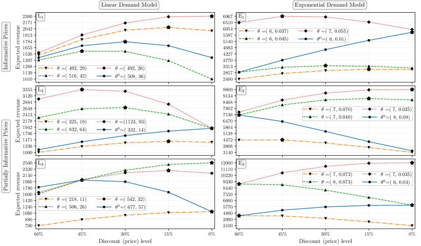
Figure 4: Revenue curves for two classes of instances.

Demand uncertainty is additive and follows a mean-zero truncated normal distribution over an interval $[-100,100]$ with a standard deviation of $\sigma$ in the set $\{5,10,15,30,60,90\}$. We vary the total number of customers $M$ in the set $\{80,400,800,1200,1600,3200\}$. Recall that $M=\sum_{t}N_{t}$. We define $N_{t}\coloneqq\left\lceil\alpha\exp(\beta(t-1))\right\rceil$ using parameters $\alpha$ and $\beta$ which can be interpreted as the scale and speed of arrivals. Choosing $\beta$ equal to zero, positive, and negative values leads to flat, exponentially increasing, and exponentially decreasing arrival patterns, respectively. We consider five arrival patterns that mimic stable, delayed-hit, and early-hit sales scenarios (see Figure 5): flat, exponentially increasing with $\beta=1.5$ and $\beta=2$, and exponentially decreasing with $\beta=-1.5$ and $\beta=-2$. Given $\beta$ and the total number of customers $M$, we compute $\alpha$ such that $\sum_{t}N_{t}=\sum_{t}\left\lceil\alpha\exp(\beta(t-1))\right\rceil$ equals $M$. By varying the parameters described above, we constructed 1080 instances for our experiments.

The revenue curves shown in Figure 4 were selected to ensure that the test instances had varying difficulty for benchmarking purposes. The first class of our instances corresponding to subplots L₁ and E₁ of Figure 4 has informative prices with respect to any uncertainty set $\mathcal{U}^{\raisebox{1.0pt}{\scaleto{\mathrm{ARL}}{4pt}}}_{t}\subseteq\Theta$, that is, all revenue curves (hence, demand curves) are well-separated by a positive margin at every price. For the second class corresponding to subplots L₂, E₂, L₃, and E₃, the optimal prices can become uninformative depending on the evolution of $\mathcal{U}^{\raisebox{1.0pt}{\scaleto{\mathrm{ARL}}{4pt}}}_{t}$. To illustrate, consider subplot L₂ of Figure 4. The four candidate demand models have revenue maximizing prices corresponding to discount levels of 0%, 15%, 30%, and 45%. If $\mathcal{U}^{\raisebox{1.0pt}{\scaleto{\mathrm{ARL}}{4pt}}}_{t}=\Theta$, 0% is partially informative because the separation between three of the revenue curves is zero at this price but there is one revenue curve that exhibits positive separation. The remaining three discount levels are informative as there is positive separation between all the demand models at these prices. If the ambiguity set is instead $\mathcal{U}^{\raisebox{1.0pt}{\scaleto{\mathrm{ARL}}{4pt}}}_{t}=\Theta\backslash\{(325,19)\}$, then a 0% discount cannot discriminate between the models in $\mathcal{U}^{\raisebox{1.0pt}{\scaleto{\mathrm{ARL}}{4pt}}}_{t}$, while 30% and 45% discounts have discriminatory power. In a nutshell, the presence of less informative prices can hamper learning as $\mathcal{U}^{\raisebox{1.0pt}{\scaleto{\mathrm{ARL}}{4pt}}}_{t}$ evolves. Partially informative instances are thus more challenging from a learning perspective.

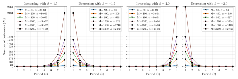
Figure 5: Different exponentially increasing and decreasing customer arrival patterns.

While price informativeness affects learning, it does not necessarily mean that misidentifying the true model leads to significant revenue loss. Under demand model ambiguity, there is significant revenue loss if the revenue-maximizing price $p^{\star}(\theta^{\prime})$ of a model with $\theta^{\prime}\neq\theta^{0}$ is such that $r_{t}(p^{\star}(\theta^{\prime});\theta^{0})\ll r_{t}(p^{\star}(\theta^{0});\theta^{0})$. We define the notion of revenue dispersion for a price $p\in\mathcal{P}$ as $(1-r_{t}(p;\theta^{0})/r_{t}(p^{\star}(\theta^{0});\theta^{0}))\times 100\%$ to account for this aspect. Specifically, we say a price has low (high) revenue dispersion if this percentage is small (large). The prices of instances L₁ and E₁ have revenue dispersion ranges of 5% to 18% and 10% to 35%, respectively. We constructed instances L₂ and E₂ so that the revenue dispersion of prices in conservative models is larger than other models. To elaborate, the average revenue dispersions for the conservative models that may be chosen by ARL are 6% and 10% for L₂ and E₂, respectively, while the analogous averages for the remaining models are 20% and 47%. The revenue dispersion varies between 17% and 45% on the instances L₃ and between 0% and 25% on the instances E₃ for all demand models (including conservative ones).

We evaluate the performance of pricing strategies using two metrics: the expected optimality gap and the 95% value at risk expressed as a percentage of the true revenue. For pricing policy $\pi$, the first metric is the difference between the expected total revenue from this policy ($\text{CI-R}(\pi)$) and the optimal expected total revenue ($\text{CI-R}(\pi^{\mathrm{CI}})$), expressed as a percentage of the latter quantity. We also define the second metric, dubbed relative value at risk (RVaR), as

$$\bigg{(}1\ -\ \text{95\% value at risk of random variable }\Big{\{}\sum_{t}N_{t}r_{t}(p_{t}^{\pi};\theta^{0})\Big{\}}\Big{/}\text{CI-R}(\pi^{\mathrm{CI}})\bigg{)}\times 100\%.$$

If RVaR of a policy $\pi$ equals $\tau\%$, then there is a 5% chance that the realized revenue from using policy $\pi$ is $\tau\%$ worse than the expected revenue from employing the complete information policy $\pi^{\mathrm{CI}}$. Thus, pricing strategies with low expected gap and RVaR are preferable since they achieve both a high expected revenue and a low revenue downside due to demand model ambiguity. We estimate both metrics by simulating policies $\pi$ and $\pi^{*}$, and generating 5000 samples from random variables $\sum_{t}N_{t}r_{t}(p_{t}^{\pi};\theta^{0})$ and $\sum_{t}N_{t}r_{t}(p_{t}^{\mathrm{CI}};\theta^{0})$. The standard error of our estimates are at most $1\%$ of the mean.

5.2 Policy Implementation

Computing ARL pricing decisions using (7) requires specifying the candidate demand model parameter set $\Theta$, which we did in §5.1. In addition, we require values for the parameters $M$, $v$, $b$, and $c$. These parameters appear in the definitions of $\Phi\left(\sum_{j=1}^{t-1}N_{j}\right)$ and $\Psi(c)$, and hence the self-adapting ambiguity set $\mathcal{U}^{\raisebox{1.0pt}{\scaleto{\mathrm{ARL}}{4pt}}}_{t}$. The parameter $M$ is known for our instances (and easily estimated in practice) since it is the total number of customer arrivals over the selling season (as opposed to demand). We sidestep the estimation of $v$, $b$, and $c$ and use a simpler approach that relies on the following assumption. It holds that $b$ equals zero, and $v$ and $c$ are such that $4(\log M)^{2}\geq 2v^{2}\log(MTc^{2}/4v^{2})$. Our assumption of $b$ equals zero is motivated by the value taken by this parameter for Gaussian distributions, while the inequality involving $v$ and $c$ is likely to hold for large $M$. Under Assumption 5.2, we have

$$\Phi\left(\sum_{j=1}^{t-1}N_{j}\right)\coloneqq\frac{2\log M}{\sqrt{\sum_{j=1}^{t-1}N_{i}}},$$ (13)

and the theory in this paper holds with minor changes. We implement ARL with this threshold.

For instances with partially informative prices, we consider an extension of ARL, dubbed ARL⁺. If at least one of the demand models in $\mathcal{U}^{\raisebox{1.0pt}{\scaleto{\mathrm{ARL}}{4pt}}}_{t}$ does not intersect with the other models at $p_{t}^{\mathrm{ARL}}$, then the prices used by the ARL⁺ and ARL policies coincide. That is, we set $p_{t}^{\mathrm{ARL}^{+}}=p_{t}^{\mathrm{ARL}}$. Otherwise, all demand models intersect at $p_{t}^{\mathrm{ARL}}$, in which case, $p_{t}^{\mathrm{ARL}^{+}}$ is computed as follows. Initialize $\hat{\mathcal{U}}_{t}=\mathcal{U}^{\raisebox{1.0pt}{\scaleto{\mathrm{ARL}}{4pt}}}_{t}$ and $\hat{p}=p_{t}^{\mathrm{ARL}}$. Remove $\hat{\theta}:=\arg\min_{\theta\in\hat{\mathcal{U}}_{t}}r_{t}(\hat{p};\theta)$ from $\hat{\mathcal{U}}_{t}$, that is, update $\hat{\mathcal{U}}_{t}=\hat{\mathcal{U}}_{t}\setminus\{\hat{\theta}\}$. Define

$$\hat{p}:=\arg\max_{p\in\mathcal{P}}\min_{\theta\in\hat{\mathcal{U}}_{t}}r_{t}(p;\theta).$$

If at least one demand model in $\mathcal{U}^{\raisebox{1.0pt}{\scaleto{\mathrm{ARL}}{4pt}}}_{t}$ does not intersect with the others at $\hat{p}$, then we set $p_{t}^{\mathrm{ARL}^{+}}=\hat{p}$. Otherwise, we repeat the steps mentioned above. Intuitively, ARL⁺ deviates from using the optimal price of the conservative revenue curves to less conservatives ones. Such a deviation occurs if optimal prices from conservative revenue curves cannot discriminate between demand models in $\mathcal{U}^{\raisebox{1.0pt}{\scaleto{\mathrm{ARL}}{4pt}}}_{t}$. We continue to use the simplified threshold (13) when implementing the ARL⁺ policy.

Finally, we describe our implementation of the SR and FTL policies. The SR policy entails solving (10), which only requires $\Theta$. In other words, no additional parameters estimation is needed. In contrast, employing FTL by solving (12) requires the choice of a prior distribution over the initial ambiguity set $\Theta$. We use a uniform prior in our numerical study.

5.3 Value of Adaptive Robustness

In this section, we compare the performance of the FTL, ARL, ARL⁺, and SR pricing policies on the instances described in §5.1.

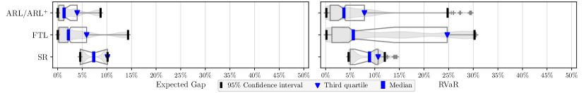
Figure 6: Performance of pricing strategies on the instances with informative prices.

Informative instances. Figure 6 depicts the distributions of the expected gap and RVaR across the informative instances in Figure 4 using a violin plot. The medians and the third quartiles of these distributions are depicted by thick blue vertical lines and triangle markers, respectively, and the thick black lines denote the 95% confidence intervals around the medians. The shaded regions above and below the horizontal line are mirror images of the density plot, with wider regions representing more likely values. Since Figure 6 reports the results on the informative instances, both ARL and ARL⁺ coincide as expected (see discussion in §5.2). The medians of the expected gap for ARL and FTL are less than 2% and the third quartiles in both cases are less than 6%. There are however instances where the expected gap of FTL is almost 15% while the analogous worst-case expected gap for ARL is around 8%. The median and third quartile of the SR expected gap (7% and 10%, respectively) are worse than the remaining methods, although its worst case expected gap across informative instances is better than FTL. These results show that ARL, which actively manages demand model ambiguity, remains competitive in terms of expected gap with FTL. The RVaR measure provides insight into the difference between ARL and FTL. The median RVaR for the former and latter methods is 3% and 6%, respectively, while analogous third quartile values are 7.5% and 25%. SR has a higher median RVaR than ARL and FTL. Its third quartile of RVaR is worse than ARL but significantly better than FTL. On the informative instances, we find that ARL reduces the risk due to model ambiguity significantly compared to both FTL and SR – self-adapting robustness in ARL thus adds significant value on the informative instances.

Figure 7: Performance of pricing strategies on the instances with partially informative prices.

Partially informative instances. Figure 7 displays the performance of the FTL and ARL pricing strategies on the partially informative instances. The expected gap distributions of ARL and SR are similar and substantially worse than the analogous distributions of ARL⁺ and FTL. We thus do not discuss ARL and SR further. For both ARL⁺ and FTL, the median and third quartile expected gaps are less than 6% and 12%, respectively. The RVaR distributions of ARL⁺ and FTL are however different with the median and the quartile of the former improving on the latter by 7% and 4%, respectively. These improvements also hold on most instances as shown in Figure 8, where we plot the difference between the RVaR of ARL⁺ and FTL. Specifically, the RVaR of ARL⁺ is better than FTL on 64% of the instances and this improvement is greater than 2% and 5% on 52% and 41% of the instances, respectively. Therefore, the adaptive robustness logic in ARL⁺ is effective at handling partially informative prices and reducing risk due to model ambiguity, while performing well in terms of expected gap.

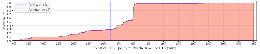
Figure 8: Distribution of the difference between ARL⁺ and FTL RVaRs on the partially informative instances.

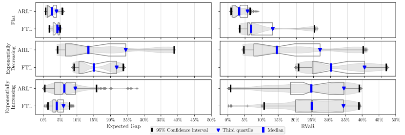
Figure 9: Impact of arrival patterns on policy performance across the partially informative instances.

Customer arrival patterns. The set of partially informative instances that we discussed thus far contain instances with three arrival patterns: flat, exponentially increasing, and exponentially decreasing. Figure 9 breaks down the performance of FTL and ARL⁺ by arrival pattern. For the flat pattern, the expected gaps of both ARL⁺ and FTL are less than 6%. Specifically, the median expected gap of ARL⁺ is smaller than that of FTL by 2%, while the third quartiles of this metric for both methods are within 0.5% of each other. In contrast, ARL⁺ significantly improves the median and the third quartile of RVaR compared to FTL by 4% and 7%, respectively. Our findings for exponentially decreasing arrivals patterns are similar in terms of ordering of methods. Here ARL⁺ is superior to FTL with respect to expected gap, although its third quartile is worse because of its skewed distribution. Unlike the flat arrival pattern, the RVaR improvement as a result of using ARL⁺ instead of FTL is substantial: median and quartile of RVaR of the former approach are 16% and 13% smaller, respectively, than the latter one. The larger RVaR improvement is because a larger number of arrivals are potentially priced suboptimally in FTL at the beginning when demand model ambiguity is high, while this risk is actively managed and mitigated in ARL⁺. These results suggest that being adaptively robust, as in ARL⁺, is likely to improve the performance of FTL in terms of both the expected gap and the RVaR on the instances with flat and exponentially decreasing arrival patterns. Indeed, one cannot always expect improvement along both metrics, as seen in our results for the exponentially increasing arrival pattern, where the median and third quartile of expected gap from FTL is better than that ARL⁺ by 2% and 4%, respectively, while the RVaR distributions of both methods essentially coincide. The intuition for this behavior is that FTL does not face significant risk of revenue loss when model ambiguity is high in the initial periods because arrivals are low, which it uses to learn the true demand model before arrivals increase. In this situation, ARL⁺ loses some revenue relative to FTL in these initial periods by being robust.

Comparison with UCB. Finally, we compare ARL⁺ with the upper confidence bound (UCB; Auer et al. 2002) algorithm. UCB is extensively used in domains such as reinforcement learning (Auer et al. 2009, Chen et al. 2017) and assortment planning (Agrawal et al. 2019, Bernstein et al. 2019), where the planning horizon is typically infinite (or long). We test the performance of UCB as a benchmark in our problem which has a relatively small number of selling/learning stages. Recall the set of revenue-maximizing prices $\mathcal{P}^{*}\equiv\cup_{\theta\in\Theta}\{\arg\max_{p\in\mathcal{P}}r_{t}(p;\theta)\}$. At period $t\in\llbracket|\mathcal{P}^{*}|\rrbracket$, the UCB policy $\pi^{\mathrm{UCB}}$ plays each price in $\mathcal{P}^{*}$ once in a uniformly random order to estimate the mean revenue from such a price. Let $p^{*}_{1},\dots,p^{*}_{|\mathcal{P}^{*}|}$ denote such a random order of the elements in $\mathcal{P}^{*}$. Then the price $p_{t}^{\mathrm{UCB}}$ employed by the UCB policy in period $t\in\llbracket|\mathcal{P}^{*}|\rrbracket$ is $p_{t}^{*}$. For a period $t\in\{|\mathcal{P}^{*}|+1,\dots,T\}$, the UCB price is defined as

$$p_{t}^{\mathrm{UCB}}\coloneqq\argmax_{p\in\mathcal{P}^{*}}\ \left\{\frac{1}{\sum_{j=1}^{t-1}\mathbbm{1}\{p_{j}^{\mathrm{UCB}}=p\}}\sum_{j=1}^{t-1}\sum_{i=1}^{N_{j}}p\mathbbm{1}\{p=p_{j}^{\mathrm{UCB}}\}d^{\mathrm{UCB}}_{ji}\ +\ \lambda\sqrt{\frac{2\log(t)}{\sum_{j=1}^{t-1}\mathbbm{1}\{p_{j}^{\mathrm{UCB}}=p\}}}\right\}$$

where $d^{\mathrm{UCB}}_{ji}$ is a shorthand for the true demand realization $d_{ji}^{\pi^{\mathrm{UCB}}}$ when using the UCB policy; $\mathbbm{1}\{\cdot\}$ is the indicator function, which evaluates to one if its argument is true and to zero otherwise; $\lambda\geq 0$ is a tunable parameter; and $\sum_{j=1}^{t-1}\sum_{i=1}^{N_{j}}p\mathbbm{1}\{p=p_{j}^{\mathrm{UCB}}\}\geq 1$ is the number of stages that price $p$ is played by the UCB policy. The term

$$\frac{1}{\sum_{j=1}^{t-1}\mathbbm{1}\{p_{j}^{\mathrm{UCB}}=p\}}\sum_{j=1}^{t-1}\sum_{i=1}^{N_{j}}p\mathbbm{1}\{p=p_{j}^{\mathrm{UCB}}\}d^{\mathrm{UCB}}_{ji}$$

is an estimate of the average revenue over the horizon $\llbracket t-1\rrbracket$ during periods in which price $p$ is played. For each instance described in §5.1, we choose $\lambda$ via cross-validation over the candidate set $\{10^{-6},10^{-5},\dots,10^{6}\}$.

Figure 10 compares ARL⁺ and UCB on our instances with exponentially increasing arrival patterns. We focus on this arrival pattern as it is favorable to UCB: playing sub-optimal prices during the first $|\mathcal{P}^{\prime}|$ stages does not translate to significant losses in total revenue due to the low volume of customers in these stages. For the informative instances, ARL⁺ improves UCB in terms of the medians of expected gap and RVaR, respectively, by 22% and 29%. For the partially informative prices, ARL⁺ improves the median expected gap of UCB by 16%, and it achieves roughly a 3% tightening of the median RVaR. Overall, ARL⁺ significantly outperforms UCB on the instances with exponentially increasing arrival patterns. The improvements of ARL⁺ over UCB are larger on the instances with flat and exponentially decreasing arrival patterns, not discussed here.

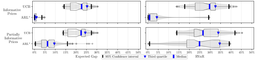
Figure 10: Performance of ARL⁺ and UCB on the instances with exponentially increasing arrival pattern.

6 Conclusion

Demand model ambiguity is a common challenge faced by retailers when setting product prices over a selling season. Suboptimal prices based on an incorrect demand model can result in revenue loss. The risk of losing revenue due to demand model ambiguity can be significant when price changes are only allowed at pre-specified time points over a finite planning horizon – a setting that arises in practice but has not been studied. We focus on this business setting. Pricing decisions based on static (distributionally) robust optimization (SR) and follow-the-leader learning (FTL) are appropriate strategies when the demand model ambiguity is either very high or very low, respectively. When model ambiguity is not at these extremes, the SR and FTL strategies can result in significant revenue losses since the former may be overly conservative while the latter minimizes regret and does not explicitly account for any risk. We thus develop an adaptively-robust-learning (ARL) pricing policy that learns the true model parameters from data while actively managing demand model ambiguity. Specifically, it maintains a stochastic set of probable models that is updated using no-regret logic to remove “unlikely” demand models in a data-driven manner. The ARL policy is robust when demand model ambiguity is high and gracefully transitions to regret-minimization when this ambiguity diminishes upon receiving more data. ARL thus bridges the gap between SR and FTL by self-adapting the level of robustness. Our analysis of ARL characterizes its stochastic behavior and shows that it exhibits favorable performance bounds. We also perform an extensive numerical study which shows that the value of adaptive robustness in ARL is substantial: compared to the SR, FTL, and UCB pricing policies, pricing decisions from ARL or an extension lead to comparable or better expected revenues and substantial improvements in the value at risk.

Electronic Companion

This online supplement reports the proofs of the statements in the paper. We provide a list of important notations in Table 1, discuss a concentration inequality that plays a centeral role in our proofs in Theorem 6.1, and prove the statements afterwards.

Table 1: Summary of notations.

$\nu,b:$	parameters of the sub-exponential distribution $D_{t}(p;\theta^{0})$ defined in Assumption 2.
$\mu_{t},r_{t}:$	the expected demand and expected revenue functions $\mu_{t}(p;\theta):=\mathbb{E}_{D}[D_{t}(p;\theta)]$ and $r_{t}(p;\theta):=p\cdot\mu_{t}(p;\theta)$.
$c:$	the separability constant defined in Assumption 2.
$m,\Theta:$	the set of all candidate demand models $\Theta=\{\theta^{0},\theta^{1},\dots,\theta^{m}\}$ with the cardinality of $m$.
$c^{(\ell)}:$	the $\ell$-th smallest $c^{i}\in\{c^{i}:i\in\llbracket m\rrbracket\}$ where $c^{i}$ (defined in 5) is the distance between models $\theta^{i}$ and $\theta^{0}$.
$N_{t},M:$	the number of arrivals in period $t$ is $N_{t}$ and the total store traffic is $M=\sum_{t=1}^{T}N_{t}$.
$p^{\pi}_{t}:$	the price taken by a policy $\pi\in\Pi$ at stage $t\in\llbracket T\rrbracket.$
$\Psi:$	$\Psi(c)=\min\left\{{c^{2}}/{8v^{2}},{c}/{4b}\right\}$.
$\Phi:$	$\Phi\big{(}\sum_{i=1}^{t-1}N_{i}\big{)}=\max\left\{{\sqrt{2v^{2}\log\big{(}2MT\Psi(c)\big{)}}}\big{/}{\sqrt{\sum_{i=1}^{t-1}N_{i}}},\ {2b\log\big{(}2MT\Psi(c)\big{)}}\big{/}{{\sum_{i=1}^{t-1}N_{i}}}\right\}$.

Theorem 6.1 (Theorem 2.3 (b) in Wainwright 2015)

Let $\{H_{k}\}_{k=1}^{\infty}$ be a martingale difference sequence with respect to filtration $\{\mathcal{H}_{k}\}_{k=1}^{\infty}$. Suppose that there exist $u,w\geq 0$ such that for every $\lambda\in(-{1}/{u},{1}/{u})$ and every $k$, it holds that

$$\mathbb{E}_{H_{k}}[\exp(\lambda H_{k})\ |\ \mathcal{H}_{k-1}]\leq\exp(\frac{\lambda^{2}w^{2}}{2})$$

almost surely. Then, for every $\zeta\geq 0$, one has that,

$$\mathbb{P}\left(\left|\sum_{k=1}^{K}H_{k}\right|\geq\zeta\right)\ \leq\ 2\exp\left(-\min\left\{\frac{\zeta^{2}}{2w^{2}K},\ \frac{\zeta}{2u}\right\}\right).$$

Proof of Theorem 3.2. Fix a policy $\pi$. Let $\mathcal{F}_{t}$ be the collection of all demand realizations collected and all pricing decisions made prior to time $t$. The stochastic process $\big{\{}\sum_{i=1}^{N_{t}}D_{ti}(p_{t}^{\pi};\theta^{0})-\mu_{t}(p_{t}^{\pi};\theta^{0})N_{t}\big{\}}_{t=1}^{\infty}$ is a martingale difference sequence with respect to filtration $\left\{\mathcal{F}_{t}\right\}_{t=1}^{\infty}$ since given the history $\mathcal{F}_{t-1}$, price $p_{t}^{\pi}$ becomes deterministic, and therefore

$$\mathbb{E}_{D,p_{t}^{\pi}}\left[\sum_{i=1}^{N_{t}}D_{ti}(p_{t}^{\pi};\theta^{0})\ -\ \mu_{t}(p_{t}^{\pi};\theta^{0})N_{t}\ \bigg{|}\ \mathcal{F}_{t-1}\right]=0,\quad\forall t=1,2,\dots,$$

where the outer expectation is taken with respect to demand random variable $D_{t}(\cdot;\theta^{0})$ and price $p_{t}^{\pi}$ that stochastically changes based on the realized samples from true demand distribution $D_{ti}(\cdot;\theta^{0})$.

Because for any $t=1,\ldots,T$ and a given $p_{t}^{\pi}\in\mathcal{P}$, random variable $D_{t}(p_{t}^{\pi};\theta^{0})$ is sub-exponential with parameters $(v,b)$, it can be seen that $D_{t}(p_{t}^{\pi};\theta^{0})-\mu_{t}(p_{t}^{\pi};\theta^{0})$ is also sub-exponential with parameters $(v,b)$, i.e., for every $\lambda\in(-{1}/{b},{1}/{b})$,

$$\mathbb{E}_{D}\left[\exp\left(\lambda\left(D_{t}(p_{t}^{\pi};\theta^{0})-\mu_{t}(p_{t}^{\pi};\theta^{0})\right)\right)\ |\ \mathcal{F}_{t-1}\right]\ \leq\ \exp(\frac{\lambda^{2}v^{2}}{2}).$$

This yields that, for every $j=1,\ldots,T$, $\sum_{i=1}^{N_{j}}D_{ji}(p_{j}^{\pi};\theta^{0})-\mu_{j}(p_{j}^{\pi};\theta^{0})N_{j}$ is sub-exponential with parameters $(v\sqrt{N_{j}},b)$. Therefore, from Theorem 6.1, one has that for any $\zeta>0$ and $t\geq 2$,

$$\mathbb{P}\left(\left|\sum_{j=1}^{t-1}\left[\sum_{i=1}^{N_{j}}D_{ji}(p_{j}^{\pi};\theta^{0})\ -\ \mu_{j}(p_{j}^{\pi};\theta^{0})N_{j}\right]\right|\geq\zeta\right)\leq 2\exp\left(-\min\left\{\frac{\zeta^{2}}{2v^{2}\sum_{j=1}^{t-1}N_{j}},\frac{\zeta}{2b}\right\}\right),$$

which is equivalent to

$$\mathbb{P}\left[\frac{\big{|}\sum_{j=1}^{t-1}[\sum_{i=1}^{N_{j}}D_{ji}(p_{j}^{\pi};\theta^{0})-\mu_{j}(p_{j}^{\pi};\theta^{0})N_{j}]\big{|}}{\sum_{j=1}^{t-1}N_{j}}\geq\zeta\right]\leq 2\exp\left[{-\sum_{j=1}^{t-1}N_{j}\min\left\{\frac{\zeta^{2}}{2v^{2}},\frac{\zeta}{2b}\right\}}\right].$$ (14)

For some $t\in\{2,3,\dots,T\}$, if $\sum_{j=1}^{t-1}N_{j}$ satisfies the condition in Definition 3.1, that is, $\sum_{j=1}^{t-1}N_{j}\geq{\log(2MT\Psi(c))}/{\Psi(c)}$, then

$$\Phi\big{(}\sum_{j=1}^{t-1}N_{j}\big{)}\leq\Phi\bigg{(}\frac{\log(2MT\Psi(c))}{\Psi(c)}\bigg{)}\leq\frac{c}{2}.$$

Hence, from inequality (14) and for $\zeta=c/2$, we have

$$\mathbb{P}\left(\frac{\big{|}\sum_{j=1}^{t-1}[\sum_{i=1}^{N_{j}}D_{ji}(p_{j}^{\pi};\theta^{0})-\mu_{j}(p_{j}^{\pi};\theta^{0})N_{j}]\big{|}}{\sum_{j=1}^{t-1}N_{j}}\leq\frac{c}{2}\right)\geq 1-2\exp\left({-\sum_{j=1}^{t-1}N_{j}\Psi(c)}\right)\geq 1-\frac{1}{MT\Psi(c)},$$

and thus with a probability of at least $1-1/(MT\Psi(c))$, we have $\xi^{\pi}_{t}(\theta^{k})\leq{c}/{2}$ for the true demand model with $k=0$, and $\xi^{\pi}_{t}\left(\theta^{k}\right)>{c}/{2}\geq\Phi\big{(}\sum_{j=1}^{t-1}N_{j}\big{)}$ for all other models with $k\geq 1$. Therefore, for any $k\geq 1$, $\theta^{k}$ will be eliminated from $\mathcal{U}^{\pi}_{t}$ with a probability of at least $1-1/(MT\Psi(c))$. $\Box$

Proof of Theorem 3.3. If for some $(i,t)\in\llbracket m\rrbracket\times\llbracket T\rrbracket$ one has $\sum_{j=1}^{t-1}N_{j}\geq{\log(2MT\Psi(c))}/{\Psi(c^{(i)})}$, then

$$\Phi\big{(}\sum_{j=1}^{t-1}N_{j}\big{)}\leq\Phi\bigg{(}\frac{\log(2MT\Psi(c))}{\Psi(c^{(i)})}\bigg{)}\leq\frac{c^{(i)}}{2}.$$

Thus, from inequality 14, we have

$$\mathbb{P}\left[\frac{\big{|}\sum_{j=1}^{t-1}[\sum_{i=1}^{N_{j}}D_{ji}(p_{j}^{\pi};\theta^{0})-\mu_{j}(p_{j}^{\pi};\theta^{0})N_{j}]\big{|}}{\sum_{j=1}^{t-1}N_{j}}\leq\frac{c^{(i)}}{2}\right]\geq 1-2\exp\left[{-\sum_{j=1}^{t-1}N_{j}\Psi(c^{(i)})}\right]\\ \geq 1-\frac{1}{MT\Psi(c)}.$$

This implies that with a probability of at least $1-{1}/(MT\Psi(c))$, we have $\xi^{\pi}_{t}(\theta^{k})\leq{c^{(i)}}/{2}$ for $k=0$ and $\xi^{\pi}_{t}(\theta^{k})>{c^{(i)}}/{2}\geq\Phi\big{(}\sum_{j=1}^{t-1}N_{j}\big{)}$ for every $k\geq i$. Therefore, for all $k\geq i$, $\theta^{k}$ will be eliminated from $\mathcal{U}^{\pi}_{t}$ with a probability of $1-1/(MT\Psi(c))$, that is, $\mathcal{U}^{\pi}_{t}\subseteq\bar{\mathcal{U}}^{\pi}_{t}$ with the same probability. $\Box$

Proof of Theorem 3.4. Consider the definition of $\tilde{t}$ in Definition 3.1. If $\tilde{t}=T+1$, that is the volume of data revealed across all $T$ periods is not sufficient for ARL to distinguish $\theta^{0}$ from the rest of demand models, then the regret of ARL is trivially bounded above by $2K_{1}\sum_{j=1}^{T}N_{j}=2K_{1}M$. Otherwise, for $\tilde{t}\in\{2,3,\dots,T\}$, it holds that

$$\text{CI-R}\left(\pi^{\mathrm{CI}}\right)\ -\ \text{CI-R}\left(\pi^{\mathrm{ARL}}\right)$$

$$\ =\sum_{t=1}^{\tilde{t}-1}\left[N_{t}r_{t}\big{(}p_{t}^{\text{CI}};\theta^{0}\big{)}-\mathbb{E}_{p_{t}^{\text{ARL}}}\big{[}N_{t}r_{t}\big{(}p_{t}^{\text{ARL}};\theta^{0}\big{)}\big{]}\right]+\sum_{t=\tilde{t}}^{T}\left[N_{t}r_{t}\big{(}p_{t}^{\text{CI}};\theta^{0}\big{)}-\mathbb{E}_{p_{t}^{\text{ARL}}}\big{[}N_{t}r_{t}\big{(}p_{t}^{\text{ARL}};\theta^{0}\big{)}\big{]}\right]$$

$$\ \leq K_{1}\sum_{t=1}^{\tilde{t}-1}N_{t}\ +\ 2K_{1}MT\exp\bigg{(}-\sum_{t=1}^{\tilde{t}-1}N_{t}\Psi(c)\bigg{)},$$ (15)

where (15) holds because $\mathbb{P}\big{(}\exists t\in\{\tilde{t},\ldots,T\}:\mathcal{U}_{t}^{\raisebox{1.0pt}{\scaleto{\pi}{2.8pt}}}\neq\{\theta^{0}\}\big{)}\leq 2T\exp\big{(}-\sum_{t=1}^{\tilde{t}-1}N_{t}\Psi(c)\big{)}$ (see the proof of Theorem 3.2 for details). By the definition of $\tilde{t}$, we have $\sum_{t=1}^{\tilde{t}-1}N_{t}\geq{\log(2MT\Psi(c))}/{\Psi(c)}$. Thus, the first term in (15) satisfies $K_{1}\sum_{t=1}^{\tilde{t}-1}N_{t}\geq K_{1}{\log(2MT\Psi(c))}/{\Psi(c)}$ and the second term in (15) satisfies $2K_{1}MT\exp({-\sum_{t=1}^{\tilde{t}-1}N_{t}\Psi(c)})\leq K_{1}/{\Psi(c)}$ by the difinition of $\tilde{t}$. Recalling Assumption 3.2, that is, $2MT\Psi(c)\geq\exp(1)$, the second term in (15) is upper bounded by the first term. Theorem 3.4 thus follows. $\Box$

Proof of Proposition 4.1. By Azuma inequality, for $\zeta>0$,

$$\mathbb{P}\bigg{(}\frac{\big{|}\sum_{j=1}^{t-1}[\sum_{i=1}^{N_{j}}D_{ji}(p_{j}^{\text{ARL}};\theta^{0})-\mu_{j}(p_{j}^{\text{ARL}};\theta^{0})N_{j}]\big{|}}{\sum_{j=1}^{t-1}N_{j}}\geq\zeta\bigg{)}\leq 2e^{-\sum_{j=1}^{t-1}N_{j}\min\big{\{}\frac{\zeta^{2}}{2v^{2}},\frac{\zeta}{2b}\big{\}}}.$$

Letting $\zeta=\Phi(\sum_{j=1}^{t-1}N_{j})$, one has that

$$\mathbb{P}\bigg{(}\frac{\big{|}\sum_{j=1}^{t-1}[\sum_{i=1}^{N_{j}}D_{ji}(p_{j}^{\text{ARL}};\theta^{0})-\mu_{j}(p_{j}^{\text{ARL}};\theta^{0})N_{j}]\big{|}}{\sum_{j=1}^{t-1}N_{j}}\geq\Phi\bigg{(}\sum_{j=1}^{t-1}N_{j}\bigg{)}\bigg{)}\leq\frac{1}{MT\Psi(c)},$$

which yields

$$\mathbb{P}\bigg{(}\xi_{t}(\theta^{0})\geq\Phi\bigg{(}\sum_{j=1}^{t-1}N_{j}\bigg{)}\bigg{)}\leq\frac{1}{MT\Psi(c)}.$$

Therefore, one has that $\theta_{0}\in\mathcal{U}^{\text{ARL}}_{t}$ with a probability of at least $1-1/(MT\Psi(c))$, which yields that for any $p\in\mathcal{P}$,

$$N_{t}r_{t}(p;\theta^{0})\geq\min_{\theta\in\mathcal{U}^{\raisebox{1.0pt}{\scaleto{\mathrm{ARL}}{4pt}}}_{t}}N_{t}r_{t}(p;\theta)$$

with a probability of at least $1-1/(MT\Psi(c))$.

On the other hand, because $\mathcal{U}^{\text{ARL}}_{t}\subseteq\Theta$, one has

$$\min_{\theta\in\mathcal{U}^{\text{ARL}}_{t}}N_{t}r_{t}(p;\theta)\geq\min_{\theta\in\Theta}N_{t}r_{t}(p;\theta).$$

Combining the two inequalities, we obtain that, for any $p\in\mathcal{P}$,

$$\Big{|}N_{t}r_{t}(p;\theta^{0})-\min_{\theta\in\mathcal{U}^{\text{ARL}}_{t}}N_{t}r_{t}(p;\theta)\big{|}\ \leq\ \big{|}N_{t}r_{t}(p;\theta^{0})-\min_{\theta\in\Theta}N_{t}r_{t}(p;\theta)\Big{|}$$

with a probability of at least $1-1/(MT\Psi(c))$. Proposition 4.1 is thus proved. $\Box$

Proof of Proposition 4.2. (a) By the definition of uncertainty set in (3), if

$$\sum_{j=1}^{t-1}N_{j}\ <\ \min_{\theta\in\Theta}\ \Phi^{-1}\left(\xi^{\text{ARL}}_{t}(\theta)\right),$$

then $\mathcal{U}^{\text{ARL}}_{t}=\Theta$ and the proof is thus complete. (b) By Theorem 3.2, one sees that for $t\geq\tilde{t}$, $\mathcal{U}^{\text{ARL}}_{t}=\{\theta^{0}\}$ with a probability of at least $1-1/(MT\Psi(c))$, which implies that $\theta_{t}^{\text{FTL}}=\theta^{0}$ with the same probability. Hence, for every period $t\in\{\tilde{t},\dots,T\}$ and price level $p\in\mathcal{P}$, it holds that,

$$\text{SR-O}_{t}(p;\Theta)\ \leq\ \text{FTL-O}_{t}(p;\theta^{\text{FTL}}_{t})\ =\ \text{ARL-O}_{t}(p;\mathcal{U}^{\raisebox{1.0pt}{\scaleto{\mathrm{ARL}}{4pt}}}_{t})\ =\text{CI-O}_{t}(p;\theta^{0}),$$

where the inequality above becomes strict if $\theta^{0}$ is not the most conservative demand model. $\Box$

Proof of Proposition 4.3. By the discussion after Theorem 3.2 and the proof of Theorem 3.2, with a probability of at least $1-2T\exp\big{(}-\sum_{j=1}^{\tilde{t}-1}N_{j}\Psi(c)\big{)}$ one has $\mathcal{U}^{\raisebox{1.0pt}{\scaleto{\mathrm{ARL}}{4pt}}}_{t}=\{\theta^{0}\}$ for any $t\geq\tilde{t}$, which further implies that ${\theta_{t}^{\text{FTL}}}=\theta^{0}$ with the same probability. If $\mathcal{U}^{\raisebox{1.0pt}{\scaleto{\mathrm{ARL}}{4pt}}}_{t}=\{\theta^{0}\}$ and ${\mathcal{\theta}}_{t}^{\text{FTL}}=\theta^{0}$, then one has $p_{t}^{\text{ARL}}=p_{t}^{\text{FTL}}$. Similar to the proof of Theorem 3.4, $|\text{CI-R}(\pi^{\text{FTL}};\theta^{0})-\text{CI-R}(\pi^{\text{ARL}};\theta^{0})|$ can be split into two terms, one term representing the revenue difference from period $1$ to $\tilde{t}-1$ and the second term from period $\tilde{t}$ to $T$. That is, for $\tilde{t}\in\{2,3,\dots,T\}$, one has

$$|\text{CI-R}\left(\pi^{\mathrm{\text{FTL}}};\theta^{0}\right)\ -\ \text{CI-R}\left(\pi^{\mathrm{ARL}};\theta^{0}\right)|$$

$$\leq\Big{|}\sum_{t=1}^{\tilde{t}-1}\big{[}\text{CI-R}_{t}\big{(}p_{t}^{\text{FTL}};\theta^{0}\big{)}-\mathbb{E}_{p_{t}^{\text{ARL}}}\big{[}\text{CI-R}_{t}\big{(}p_{t}^{\text{ARL}};\theta^{0}\big{)}\big{]}\big{]}\Big{|}+\Big{|}\sum_{t=\tilde{t}}^{T}\big{[}\text{CI-R}_{t}\big{(}p_{t}^{\text{FTL}};\theta^{0}\big{)}-\mathbb{E}_{p_{t}^{\text{ARL}}}\big{[}\text{CI-R}_{t}\big{(}p_{t}^{\text{ARL}};\theta^{0}\big{)}\big{]}\big{]}\Big{|}$$

$$\leq K_{1}\sum_{t=1}^{\tilde{t}-1}N_{t}\ +\ 2K_{1}MT\exp\bigg{(}-\sum_{t=1}^{\tilde{t}-1}N_{t}\Psi(c)\bigg{)}.$$ (16)

Therefore, by the same reasoning as in the proof of Theorem 3.4, Proposition 4.3 can be proved. $\Box$

Proof of Corollary 4.4. Note that when this condition is satisfied, two metrics $\text{ARL-R}_{t}(\cdot;\mathcal{U}^{\raisebox{1.0pt}{\scaleto{\mathrm{ARL}}{4pt}}}_{t})$ and $\text{SR-R}_{t}(\cdot;\Theta)$ coincide at every time $t\in\llbracket T\rrbracket$ due to Proposition 4.2(a). Consequently, $p_{t}^{\text{ARL}}=p_{t}^{\text{SR}}$ for any $t\in\llbracket T\rrbracket$. Corollary 4.4 thus follows by definition. $\Box$

References

- Agrawal et al. (2019) Agrawal S, Avadhanula V, Goyal V, Zeevi A (2019) Mnl-bandit: A dynamic learning approach to assortment selection. Operations Research 67(5):1453–1485.
- Araman and Caldentey (2010) Araman VF, Caldentey R (2010) Revenue management with incomplete demand information. Wiley Encyclopedia of Operations Research and Management Science .
- Auer et al. (2002) Auer P, Cesa-Bianchi N, Fischer P (2002) Finite-time analysis of the multiarmed bandit problem. Machine learning 47(2-3):235–256.
- Auer et al. (2009) Auer P, Jaksch T, Ortner R (2009) Near-optimal regret bounds for reinforcement learning. Advances in neural information processing systems, 89–96.
- Ben-Tal et al. (2013) Ben-Tal A, Den Hertog D, De Waegenaere A, Melenberg B, Rennen G (2013) Robust solutions of optimization problems affected by uncertain probabilities. Management Science 59(2):341–357.
- Bernstein et al. (2019) Bernstein F, Modaresi S, Sauré D (2019) A dynamic clustering approach to data-driven assortment personalization. Management Science 65(5):2095–2115.
- Bertsimas et al. (2018) Bertsimas D, Gupta V, Kallus N (2018) Robust sample average approximation. Mathematical Programming 171(1-2):217–282.
- Besbes and Zeevi (2009) Besbes O, Zeevi A (2009) Dynamic pricing without knowing the demand function: Risk bounds and near-optimal algorithms. Operations Research 57(6):1407–1420.
- Besbes and Zeevi (2012) Besbes O, Zeevi A (2012) Blind network revenue management. Operations Research 60(6):1537–1550.
- Besbes and Zeevi (2015) Besbes O, Zeevi A (2015) On the surprising sufficiency of linear models for dynamic pricing with demand learning. Management Science 61(4):723–739.
- Bitran and Caldentey (2003) Bitran G, Caldentey R (2003) An overview of pricing models for revenue management. Manufacturing & Service Operations Management 5(3):203–229.
- Blum (1998) Blum A (1998) On-line algorithms in machine learning. Online algorithms, 306–325 (Springer).
- Bu et al. (2020) Bu J, Simchi-Levi D, Wang L (2020) Offline pricing and demand learning with censored data. Available at SSRN 3619625 .
- Chen et al. (2019a) Chen B, Chao X, Ahn HS (2019a) Coordinating pricing and inventory replenishment with nonparametric demand learning. Operations Research 67(4):1035–1052.
- Chen et al. (2019b) Chen B, Chao X, Shi C (2019b) Nonparametric learning algorithms for joint pricing and inventory control with lost-sales and censored demand. Mathematics of Operations Research, forthcoming .
- Chen and Chen (2015) Chen M, Chen ZL (2015) Recent developments in dynamic pricing research: multiple products, competition, and limited demand information. Production and Operations Management 24(5):704–731.
- Chen et al. (2019c) Chen Q, Jasin S, Duenyas I (2019c) A nonparametric self-adjusting control for joint learning and optimization of multi-product pricing with finite resource capacity. Mathematics of Operations Research 44(2):601–631.
- Chen et al. (2017) Chen RY, Schulman J, Abbeel P, Sidor S (2017) Ucb and infogain exploration via q-ensembles. arXiv preprint arXiv:1706.01502 9.
- Cheung et al. (2017) Cheung WC, Simchi-Levi D, Wang H (2017) Dynamic pricing and demand learning with limited price experimentation. Operations Research 65(6):1722–1731.
- Chollet (2019) Chollet F (2019) On the measure of intelligence. arXiv preprint arXiv:1911.01547 .
- DeepMind (2017) DeepMind (2017) Alphago zero: Starting from scratch. Technical report, DeepMind, URL https://deepmind.com/blog/article/alphago-zero-starting-scratch.
- Delage and Ye (2010) Delage E, Ye Y (2010) Distributionally robust optimization under moment uncertainty with application to data-driven problems. Operations research 58(3):595–612.
- den Boer and Keskin (2019) den Boer A, Keskin NB (2019) Dynamic pricing with demand learning and reference effects. Available at SSRN 3092745 .
- den Boer (2015) den Boer AV (2015) Dynamic pricing and learning: historical origins, current research, and new directions. Surveys in operations research and management science 20(1):1–18.
- Elmaghraby and Keskinocak (2003) Elmaghraby W, Keskinocak P (2003) Dynamic pricing in the presence of inventory considerations: Research overview, current practices, and future directions. Management science 49(10):1287–1309.
- Esfahani and Kuhn (2018) Esfahani PM, Kuhn D (2018) Data-driven distributionally robust optimization using the wasserstein metric: Performance guarantees and tractable reformulations. Mathematical Programming 171(1-2):115–166.
- Feng and Shanthikumar (2018) Feng Q, Shanthikumar JG (2018) How research in production and operations management may evolve in the era of big data. Production and Operations Management 27(9):1670–1684.
- Foss et al. (2011) Foss S, Korshunov D, Zachary S, et al. (2011) An introduction to heavy-tailed and subexponential distributions, volume 6 (Springer).
- Goh and Sim (2010) Goh J, Sim M (2010) Distributionally robust optimization and its tractable approximations. Operations research 58(4-part-1):902–917.
- Gupta (2019) Gupta V (2019) Near-optimal bayesian ambiguity sets for distributionally robust optimization. Management Science 65(9):4242–4260.
- Kalai and Vempala (2005) Kalai A, Vempala S (2005) Efficient algorithms for online decision problems. Journal of Computer and System Sciences 71(3):291–307.
- Lei et al. (2019) Lei Y, Jasin S, Sinha A (2019) Near-optimal bisection search for nonparametric dynamic pricing with inventory constraint, working paper, University of Michigan, Ann Arbor, MI.
- McKinsey (2016) McKinsey (2016) Omnichannel compendium for retailers. Technical report, URL https://www.mckinsey.com/business-functions/marketing-and-sales/solutions/periscope/our-insights/articles/omnichannel-compendium-for-retailers.
- Pakiman et al. (2020) Pakiman P, Nadarajah S, Soheili N, Lin Q (2020) Self-guided approximate linear programs. Available at SSRN .
- Pflug and Wozabal (2007) Pflug G, Wozabal D (2007) Ambiguity in portfolio selection. Quantitative Finance 7(4):435–442.
- Scarf (1958) Scarf H (1958) A min-max solution of an inventory problem. Studies in the mathematical theory of inventory and production .
- Shah et al. (2020) Shah D, Somani V, Xie Q, Xu Z (2020) On reinforcement learning for turn-based zero-sum markov games. arXiv preprint arXiv:2002.10620 .
- Shalev-Shwartz et al. (2011) Shalev-Shwartz S, et al. (2011) Online learning and online convex optimization. Foundations and trends in Machine Learning 4(2):107–194.
- Silver et al. (2017) Silver D, Hubert T, Schrittwieser J, Antonoglou I, Lai M, Guez A, Lanctot M, Sifre L, Kumaran D, Graepel T, et al. (2017) Mastering chess and shogi by self-play with a general reinforcement learning algorithm. arXiv preprint arXiv:1712.01815 .
- Wang et al. (2020) Wang Y, Chen B, Simchi-Levi D (2020) Multi-modal dynamic pricing. Available at SSRN 3489355 .
- Wang et al. (2014) Wang Z, Deng S, Ye Y (2014) Close the gaps: A learning-while-doing algorithm for single-product revenue management problems. Operations Research 62(2):318–331.
- Wiesemann et al. (2014) Wiesemann W, Kuhn D, Sim M (2014) Distributionally robust convex optimization. Operations Research 62(6):1358–1376.
- Windstream Enterprise (2020) Windstream Enterprise (2020) The future of unified commerce. Technical report, URL https://www.windstreamenterprise.com/wp-content/uploads/2020/08/the-future-of-unified-commerce-insights-paper.pdf.
- Zhang and Jasin (2018) Zhang H, Jasin S (2018) Online learning and optimization of (some) cyclic pricing policies in the presence of patient customers. Available at SSRN 3144018 .

References

- Wainwright (2015) Wainwright M (2015) Course on mathematical statistics, chapter 2: Basic tail and concentration bounds. University of California at Berkeley, Department of Statistics.